Embed Size (px)
Citation preview
GMV-PID Controller Design with Gradient Method for the
Energy Weighting Factor in Nonlinear Plants
Antonio S. Silveira*, Antonio A. R. Coelho*, Francisco J. Gomes**
* Federal University of Santa Catarina, Department of Automation and Systems, 88040900
Florianópolis, SC, Brazil (e-mail: [email protected], [email protected])
** Federal University of Juiz de Fora, Faculty of Engineering, 36036330
Juiz de Fora, MG, Brazil (e-mail: [email protected])
Abstract: Since the PID tuning formula of Ziegler-Nichols step test, perhaps the best known, the process
control literature is still showing lots of PID control schemes to improve the closed-loop stability. In this
paper, using the relationship between the PID and generalized minimum variance (GMV) controller and
adjusting online the control weighting factor by an adaptive learning algorithm of first-order (gradient
method), a new control design is investigated. Besides, the control algorithm is gathering the direct
estimation technique, with the covariance resetting procedure based on the weighted prediction error, to
deal with nonlinear plants. Numerical and practical experiments are shown to evaluate the behavior of the
proposed GMV-PID control design.
Keywords: PID controllers, minimum variance control, optimal search techniques, adaptive algorithms,
numerical simulation, gradient methods, asymptotic stability.
1. INTRODUCTION
The importance of the PID controller in the industry is related
to factors such as simplicity, stability and performance. At
least three parameters must be set and sometimes they need
an online retuning in complex environments, i.e., due to plant
parameters variations (Åström and Hägglund, 2006; Visioli,
2006; Gude et al., 2006). Depending on the cleverness of the
operator, the parameter tuning procedure can vary from
seconds to hours, especially for slow dynamic or in nonlinear
plants. To deal with these real loop situations, it is possible to
find, in books and conference papers, many automatic tuning
approaches where success and failure cases are reported in
the following industries: chemical, petrochemical,
metallurgy, pulp and paper, electrical, mechanical, etc. (Ang
et al., 2005). In this scenario there are projects related to the
PID tuning where the combination with other control
strategies are applied in order to guarantee the robustness of
the control loop. Internal Model Control (IMC) and
Generalized Minimum Variance (GMV) control
methodologies are of great importance because they can
acquire different closed-loop characteristics such as model
reference, detuned behavior and time-delay compensation
(Gude et al. 2006; Veronesi and Visioli, 2011). A good
example is the work of Cameron and Seborg (1983)
hybridizing the GMV design with the PID tuning, where
excessive actuator movements can be avoided and non-
minimum phase plants can be controlled. However, due to the
fixed tuning, the performance of GMV-PID controller can
degrade or even become unstable when applied to nonlinear
processes. In addition, self-tuning control strategies are
becoming conventional methods and a considerable number
of successful experimental studies have been carried out in
PID and GMV over the last years (Doi and Mori, 2002;
Hägglund and Åström, 2000; Kirecci et al., 2003). The idea
of using direct parameter estimation is good because the
GMV-PID linear controller design is based on a linear model
that is obtained in the operating point vicinity and the
performance specifications is not guaranteed in the whole
operating range. To avoid the drawback of fixed GMV-PID
parameters damaging the transient response, a gradient
method is combined into the GMV-PID framework.
Therefore in this paper, the adaptive character is implemented
by means of two online adjustable ways: direct estimation of
the GMV-PID parameters and learning method to optimize
the energy weighting factor of the controller. The direct
GMV-PID control design proposed in this paper differs from
the existing GMV-PID controller of Cameron and Seborg
(1983) and Yamamoto et al. (1999), where they only employ
a recursive algorithm to identify the controlled plant
parameters. The process response and control signal can be
visualized from simulations with the proposed control-loop
strategy. Comparison with conventional tuning sets is done.
2. GMV BASED PID CONTROLLER DESIGN
2.1 Process Description
Many experimental plants can be well described by the
following First-Order Plus Dead-Time (FOPDT) model
(Åström and Hägglund (2006):
1s
eK)s(G
)s(U
)s(Ys
p
m
(1)
IFAC Conference on Advances in PID Control PID'12 Brescia (Italy), March 28-30, 2012 ThB1.3
where Kp, and θ denote the process gain, time-constant and
time-delay, respectively. In order to ensure a second-order
model for controller design purpose, it is possible to use a
first-order lag element for the time-delay and (1) can be
rewritten as
)1s)(1s(
K)s(G
p
m
(2)
The discrete-time model, obtained from (2), called Controlled
Auto-Regressive (CAR) model, is given by
)t()t(u)z(Bz)t(y)z(A 111 (3)
where
22
11
1 zaza1)z(A ; 110
1 zbb)z(B (4)
and y(t), u(t) and (t) are the process output, control input and
white noise. Furthermore, z-1 denotes the backward shift
operator, namely, z-1y(t) = y(t-1).
2.2 PID Controller Structure
The following digital PID control law, in parallel form, is
considered (Bobál et al., 2005; Visioli, 2006):
)]2t(e)1t(e2
)t(e[K)t(eK)]1t(e)t(e[K)t(u dic
(5)
where Kc, Ki and Kd are the tuning parameters and represent
the proportional, integral and derivative gains, respectively.
In addition, e(t) = yr(t) – y(t) is the system error and yr(t) is
the reference signal. Assuming that the reference appears
only in the integral part and the output is filtered, yf(t), then
for the GMV control design, (5) is modified and can be
rewritten as
)2t(yK)1t(y)K2K(
)t(y)KKK()t(yK)t(u
fdfdc
fdicri
(6)
The closed-loop system performance strongly depends on
PID parameters. These parameters can be computed with the
GMV-PID control tuning scheme, which have been already
proposed by Cameron and Seborg (1983) and Yamamoto et
al. (1998), using the trial and error procedure. However, due
to the difficult to tune a design parameter of the GMV, that
weights the energy of the control signal, and to avoid a fixed
value that can be unfeasible in nonlinear essays, this paper
proposes an on-line adaptive learning procedure to estimate it
that is desirable as a systematic way for practical
applications.
2.3 GMV Based PID Parameter Tuning
The derivation of GMV-PID controller proposed in Cameron
and Seborg (1983) is reviewed. To design the GMV
controller it is assumed that the monovariable controlled
system is modelled by (3) and, additionally, an auxiliary
output is defined as follows:
)1t(y)z(R)1t(u)z(Q)t(y)z(P)t( r111 (7)
with P(z-1), Q(z-1) and R(z-1) being weighting polynomials. If
the input-output data are known until time t, the (t+1) can
be regarded as estimating y(t+1) by
)1t(y)z(P)1t( 1y
)1t()z(E)t(u)z(B)z(E)t(y)z(P
)z(F)1t( 111
1d
1
y
(8)
where E(z-1) and F(z-1) are obtained by the identity
)z(P)z(A
)z(Fz)z(E
)z(P)z(A
)z(P1
d1
111
1d
1
1n
with Pn(z-1)/Pd(z
-1) = P(z-1). Assuming G(z-1) = E(z-1)B(z-1)
then (8) is rewritten as follows:
)t()t(u)z(G)t(y)z(F)1t( 1f
1y (9)
where (t) = E(z-1)ξ(t+1) and yf(t) is the filtered output
defined by
)t(y)zp1(
)p1()t(y
)z(P
1)t(y
11d
1d
1d
f
; 1p0 1d
Therefore, from (7) and (9) and forcing to zero the
deterministic part of (t+1), the GMV control law is given by
)z(Q)z(G
)t(y)z(F)t(y)z(R)t(u
11
f1
r1
(10)
To ensure that the GMV in (10) has the PID structure of (6) it
is necessary to define the polynomials F(z-1) and R(z-1) as
22
110
1 zfzff)z(F (11)
2
0i
id
1 f)1(P
)1(F)1(H)z(R (12)
The derivation of R(z-1) = H(1) is to ensure steady-state
agreement between output and reference signals. As the final
design step, the integral action must be introduced by setting
the Q(z-1) polynomial as
)z(G)z1(
)z(Q 11
1
(13)
where is a design parameter. If (12) and (13) are
substituted into (10), then the corresponding settings of the
GMV-PID control law are expressed as
)]t(y)z(F)t(Hy[)t(u f1
r (14)
IFAC Conference on Advances in PID Control PID'12 Brescia (Italy), March 28-30, 2012 ThB1.3
)f2f(K 21c ; )fff(K 210i ; 2d fK (15)
The choice of modifies the closed-loop behavior of the
controlled system. Large values of will tend to result in
more vigorous control and underdamped responses while
small values of will tend to provide more sluggish control
and overdamped responses. Therefore for real applications, it
is desirable to have a systematic approach for obtaining an
adequate value of , avoiding the time-consuming trial and
error procedure, that sometimes sets an inadequate value
which may lead to an unstable dynamic.
2.4 Optimizing the Weighting Factor of the GMV-PID
Controller
To tune the design parameter of (14), which is constrained
between 0 and 1, a sigmoid function is employed to map the
space [0 1] to the entire real number space as follows:
)t(e1
1)t(
(16)
with (t) being a real number. Using (16) the parameter (t)
is calculated updating (t) according to the gradient method,
such that
)t(
J)t()t()1t(
(17)
where the parameter (t) = 0/t (0 < 0 < max) regulates the
stability, convergence velocity and must be selected for each
application. The cost function J has the form
2
2yr
1
)]1t(u)t(u[
)]1t()1t(y)z(P[)1t(J
(18)
with λ as the weighting parameter. In order to calculate the
gradient J/(t) the chain rule is applied as follows:
)t(
)t(
)t(
)t(u
)t(u
J
)t(
J
(19)
where
)]1t(u)t(u[2)t(u
)1t()]1t(u)z(G
)t(y)z(F)1t(y)z(P[2)t(u
J
y1
f1
r1
(20)
]g)z(G[z)z(G 011 ; 0
yg
)t(u
)1t(
)t(y)zf()t(y)f()t(
)t(u2
0i
iir
2
0i
i
(21)
)]t(1)[t()t(
)t(
(22)
2.5 Updating the Weighting Factor with Cameron-Seborg
Tuning
The scalar parameter (t), in (14), provides a convenient
tuning parameter for the GMV-PID controller. For practical
applications, it is desirable to have a satisfactory initial
estimation procedure before actually implementing the digital
control signal. So, for the purpose of comparison, the
Cameron and Seborg (1983) tuning method is employed as
the standard control design. Then, (t) can be well tuned
based on the discrete model of (1) such as
11
0)1d(
pza1
bz)z(G
(23)
where )a1(Kb 1p0 , )/Texp(a s1 , sT/d and Ts
is the sampling period. Cameron and Seborg (1983) have
demonstrated that, based on the characteristic equation and
the Jury stability method, the maximum value of (t), to
guarantee closed-loop stability for d = 0 and d = 1, is given,
respectively, by
)a1(aK
)a1(2
11p
1max
(24)
21p
maxaK
1
In practical applications, it is desirable that the estimated
value of (t) be conservative to avoid closed-loop dynamics
with oscillatory or unstable behavior. Hence Cameron and
Seborg (1983) have recommended that (t) = βvmax (t) be
used where 0 < β < 1. A value of β = 0.1 or β = 0.2 can
provide a satisfactory calibration for (t) if the process is
open-loop stable.
2.6 Direct Adaptive Estimation of the GMV-PID Controller
For the GMV-PID control law synthesis, in the direct
adaptive framework, a parametric estimation scheme is based
on the recursive least-squares algorithm with covariance
resetting. The estimator is derived from (9) assuming that
F(z-1) = f0 + f1z-1 + f2z
-2 and G(z-1) = g0 + g1z-1. Parameters
and measurements vectors are given by
]ggfff[)t( 10210T
(25)
)]2t(u)1t(u)3t(y)2t(y)1t(y[)t(T
and the estimated parameters are updated using the standard
recursive least-squares estimator
IFAC Conference on Advances in PID Control PID'12 Brescia (Italy), March 28-30, 2012 ThB1.3
)]1t()t()t(y)[t(K)1t()t( T
)t()1t(P)t(1
)t()1t(P)t(K
T
(26)
)t()1t(P)t(1
)1t(P)t()t()1t(P)1t(P)t(P
T
T
where K(t) and P(t) are the estimator gain and covariance
matrix, respectively. To deal with inaccuracy, robustness,
interactions between the estimator-controller and time-
varying plants, the covariance resetting procedure is
employed. Hence, the covariance matrix is calculated in the
traditional way, i.e., P(t) = P(t) + Q(t). The reset of P(t) is
based on the weighted prediction error which is determined
as follows:
e
e
N
1i
N
1i
est
reset
)i(
)1it(e)i(
)t(error (27)
with )1t()t()t(y)t(e Test . At every discrete-time
instant, a moving window of Ne values is used to calculate the
weighted prediction error and the matrix Q(t) is added only
when the weighted prediction error value exceeds a tolerance
error, etol, given by the user. This kind of behavior is
appropriate not only to reduce undesirable covariance
resetting due to process noise but also to provide good
accuracy for tracking time-varying parameters.
3. NUMERICAL AND EXPERIMENTAL SIMULATIONS
The effectiveness of the proposed adaptive GMV-PID
controller is assessed on two simulation examples. As the
first essay, a linear time-invariant plant is given by the
following equation:
4p)1s(
1)s(G
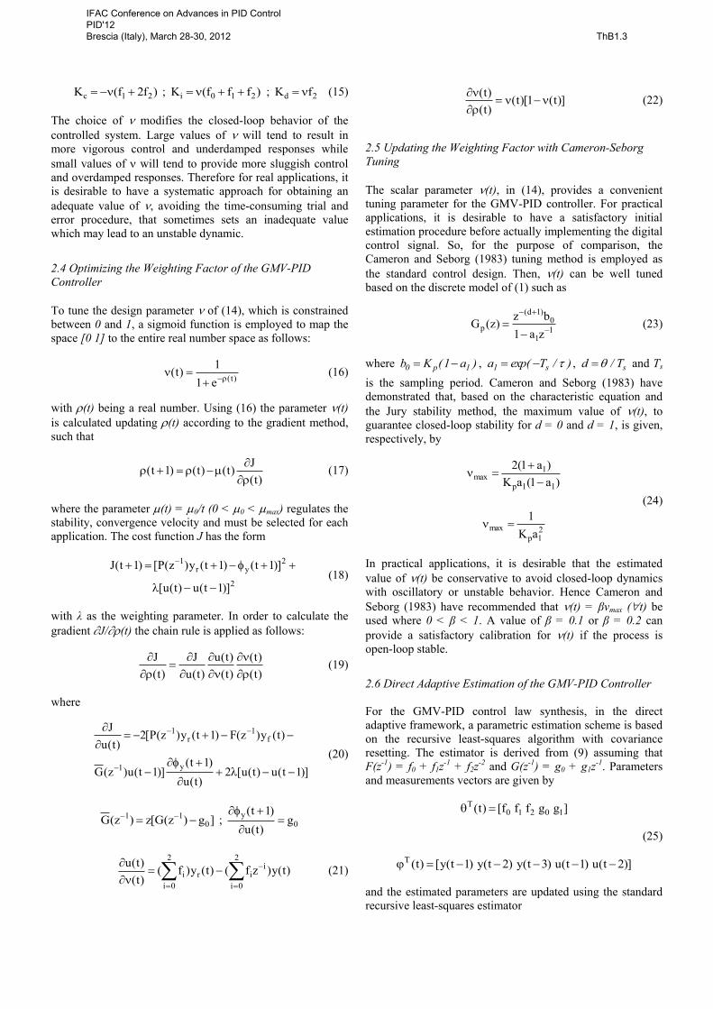
User specified parameters are set to P(0) = 200I5x5, θ(0) =
0.01, P(z-1) = 1, (0) = 1, (0) = 0, max = 20, λ = 2 and Ts =
1 s. The behavior of the closed-loop system, for two setpoint
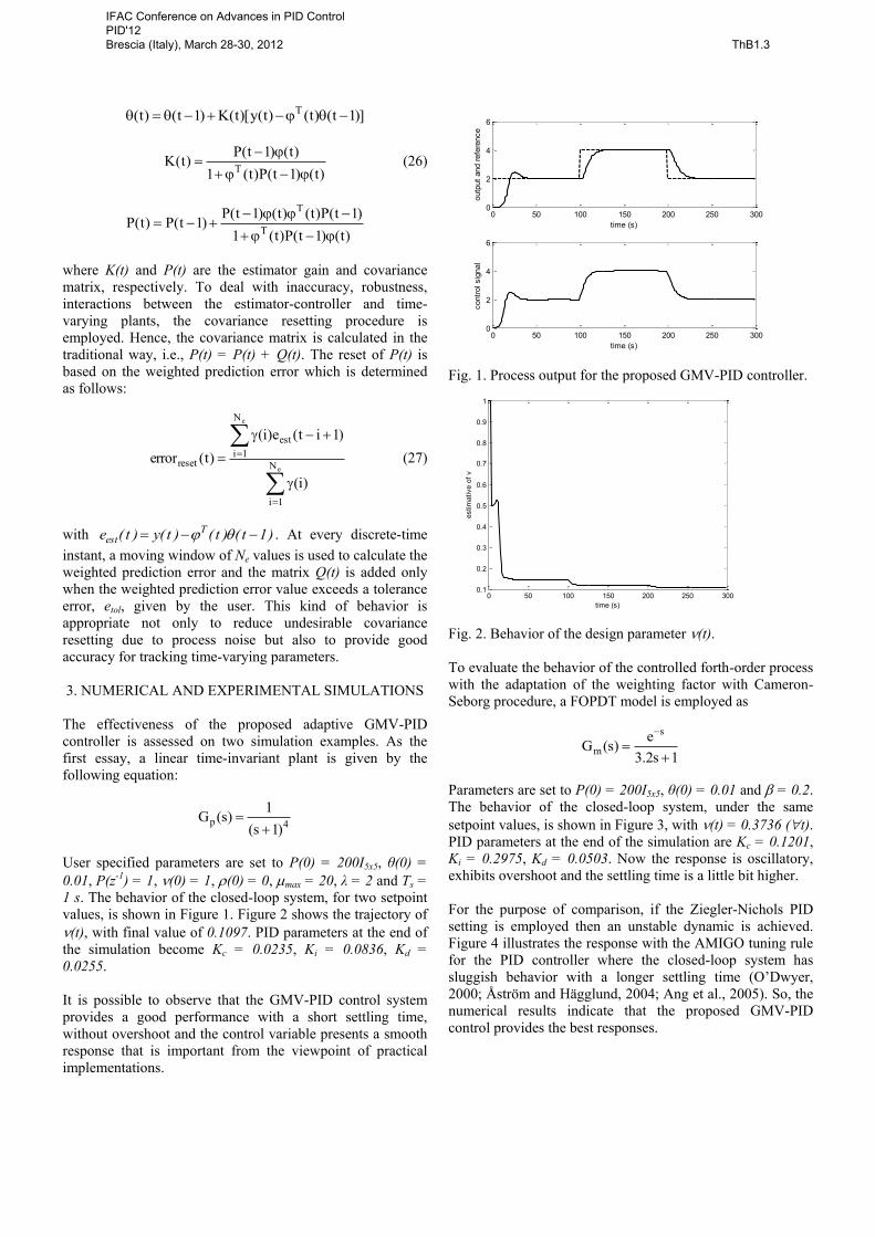
values, is shown in Figure 1. Figure 2 shows the trajectory of
(t), with final value of 0.1097. PID parameters at the end of
the simulation become Kc = 0.0235, Ki = 0.0836, Kd =
0.0255.
It is possible to observe that the GMV-PID control system
provides a good performance with a short settling time,
without overshoot and the control variable presents a smooth
response that is important from the viewpoint of practical
implementations.
0 50 100 150 200 250 3000
2
4
6
outp
ut
and r
efe
rence
time (s)
0 50 100 150 200 250 3000
2
4
6
contr
ol sig
nal
time (s)
Fig. 1. Process output for the proposed GMV-PID controller.
0 50 100 150 200 250 3000.1
0.2
0.3
0.4
0.5
0.6
0.7
0.8
0.9
1
estim
ative o
f v
time (s)
Fig. 2. Behavior of the design parameter (t).
To evaluate the behavior of the controlled forth-order process
with the adaptation of the weighting factor with Cameron-
Seborg procedure, a FOPDT model is employed as
1s2.3
e)s(G
s
m
Parameters are set to P(0) = 200I5x5, θ(0) = 0.01 and = 0.2.
The behavior of the closed-loop system, under the same
setpoint values, is shown in Figure 3, with (t) = 0.3736 (t).
PID parameters at the end of the simulation are Kc = 0.1201,
Ki = 0.2975, Kd = 0.0503. Now the response is oscillatory,
exhibits overshoot and the settling time is a little bit higher.
For the purpose of comparison, if the Ziegler-Nichols PID
setting is employed then an unstable dynamic is achieved.
Figure 4 illustrates the response with the AMIGO tuning rule
for the PID controller where the closed-loop system has
sluggish behavior with a longer settling time (O’Dwyer,
2000; Åström and Hägglund, 2004; Ang et al., 2005). So, the
numerical results indicate that the proposed GMV-PID
control provides the best responses.
IFAC Conference on Advances in PID Control PID'12 Brescia (Italy), March 28-30, 2012 ThB1.3
0 50 100 150 200 250 3000
2
4
6
outp
ut
and r
efe
rence
time (s)
0 50 100 150 200 250 3000
2
4
6
contr
ol sig
nal
time (s)
Fig. 3. Output for the GMV PID tuned by Cameron-Seborg.
0 50 100 150 200 250 3000
2
4
6
outp
ut
and r
efe
rence
time (s)
0 50 100 150 200 250 3000
2
4
6
contr
ol sig
nal
time (s)
Fig. 4. Output for the PID controller tuned by AMIGO.
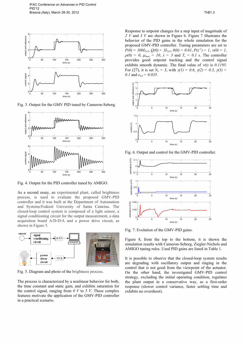
As a second essay, an experimental plant, called brightness
process, is used to evaluate the proposed GMV-PID
controller and it was built at the Department of Automation
and Systems/Federal University of Santa Catarina. The
closed-loop control system is composed of a light sensor, a
signal conditioning circuit for the output measurement, a data
acquisition board A/D-D/A and a power drive circuit, as
shown in Figure 5.
Fig. 5. Diagram and photo of the brightness process.
The process is characterized by a nonlinear behavior for both,
the time constant and static gain, and exhibits saturation for
the control signal, ranging from 0 V to 5 V. These complex
features motivate the application of the GMV-PID controller
in a practical scenario.
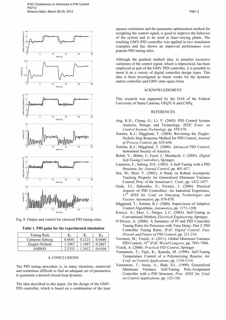
Response to setpoint changes for a step input of magnitude of
2 V and 3 V are shown in Figure 6. Figure 7 illustrates the
behavior of the PID gains in the whole simulation for the
proposed GMV-PID controller. Tuning parameters are set to
P(0) = 300I5x5, Q(0) = 3I5x5, θ(0) = 0.01, P(z-1) = 1, (0) = 1,
(0) = 0, max = 10, λ = 3 and Ts = 0.1 s. The controller
provides good setpoint tracking and the control signal
exhibits smooth dynamic. The final value of (t) is 0.1195.
For (27), it is set Ne = 3, with (1) = 0.6, (2) = 0.3, (3) =
0.1 and etol = 0.035.
0 5 10 15 20 250
1
2
3
4
outp
ut
and r
efe
rence (
V)
time (s)
0 5 10 15 20 250
0.5
1
1.5
contr
ol (V
)
time (s)
Fig. 6. Output and control for the GMV-PID controller.
0 5 10 15 20 25-0.1
0
0.1
estim
ative o
f K
c
time (s)
0 5 10 15 20 250
0.5
1
estim
ative o
f K
i
time (s)
0 5 10 15 20 250
0.02
0.04
estim
ative o
f K
d
time (s)
Fig. 7. Evolution of the GMV-PID gains.
Figure 8, from the top to the bottom, it is shown the
simulation results with Cameron-Seborg, Ziegler-Nichols and
AMIGO tuning rules. Used PID gains are listed in Table 1.
It is possible to observe that the closed-loop system results
are degrading with oscillatory output and ringing in the
control that is not good from the viewpoint of the actuator.
On the other hand, the investigated GMV-PID control
strategy, excluding the initial operating condition, regulates
the plant output in a conservative way, as a first-order
response (slower control variance, faster settling time and
exhibits no overshoot).
IFAC Conference on Advances in PID Control PID'12 Brescia (Italy), March 28-30, 2012 ThB1.3
0 5 10 15 20 250
1
2
3
4
outp
ut
and r
efe
rence (
V)
time (s)
0 5 10 15 20 250
0.5
1
1.5
contr
ol (V
)
time (s)
0 5 10 15 20 250
1
2
3
4
outp
ut
and r
efe
rence (
V)
time (s)
0 5 10 15 20 250
1
2
3
contr
ol (V
)
time (s)
0 5 10 15 20 250
1
2
3
4
outp
ut
and r
efe
rence (
V)
time (s)
0 5 10 15 20 250
1
2
3
contr
ol (V
)
time (s)
Fig. 8. Output and control for classical PID tuning rules.
Table 1. PID gains for the experimental simulation
Tuning Rule Kc Ki Kd
Cameron-Seborg 0.0841 0.2123 0.0440
Ziegler-Nichols 1.1067 1.1067 0.2667
AMIGO 2.5333 1.3412 0.6104
4. CONCLUSIONS
The PID tuning procedure is, in many situations, nontrivial
and sometimes difficult to find an adequate set of parameters
to guarantee a desired closed-loop dynamic.
The idea described in this paper, for the design of the GMV-
PID controller, which is based on a combination of the least
squares estimation and the parameter optimization method for
weighting the control signal, is good to improve the behavior
of the system and to be used in time-varying plants. The
resulting GMV-PID controller was applied in two simulation
examples and has shown an improved performance over
popular PID tuning rules.
Although the gradient method idea, to penalize excessive
variations of the control signal, which is impractical, has been
employed as part of the GMV-PID controller, it is possible to
insert it on a variety of digital controller design types. This
idea is been investigated as future works for the dynamic
matrix controller and GMV state-space form.
ACKNOWLEDGMENT
This research was supported by the DAS of the Federal
University of Santa Catarina, GPqTCA and CNPq.
REFERENCES
Ang, K.H.; Chong, G.; Li, Y. (2005). PID Control System
Analysis, Design, and Technology, IEEE Trans. on
Control Systems Technology, pp. 559-576.
Åström, K.J.; Hägglund, T. (2004). Revisiting the Ziegler-
Nichols Step Response Method for PID Control, Journal
of Process Control, pp. 635-650.
Åström, K.J.; Hägglund, T. (2006). Advanced PID Control,
Instrument Society of America.
Bobál, V.; Böhm, J.; Fessl, J.; Machácek, J. (2005). Digital
Self-Tuning Controllers, Springer.
Cameron, F.; Seborg, D.E. (1983). A Self-Tuning with a PID
Structure, Int. Journal Control, pp. 401-417.
Doi, M.; Mori, Y. (2002). A Study on Robust Asymptotic
Tracking Property for Generalized Minimum Variance
Control, Proc. of the American C. Conf., pp. 1472-1477.
Gude, J.J.; Hahoraho, E.; Etxaniz, J. (2006). Practical
Aspects of PID Controllers: An Industrial Experience,
11th IEEE Int. Conf. on Emerging Technologies and
Factory Automation, pp. 870-878.
Hägglund, T.; Åström, K.J. (2000). Supervision of Adaptive
Control Algorithms, Automatica, pp. 1171-1180.
Kirecci, A.; Eker, I.; Dulger, L.C. (2003). Self-Tuning as
Conventional Method, Electrical Engineering, Springer.
O’Dwyer, A. (2000). A Summary of PI and PID Controller
Tuning Rules for Processes with Time Delay. Part 2: PID
Controller Tuning Rules, IFAC Digital Control: Past,
Present and Future of PID Control, pp. 211-216.
Veronesi, M.; Visioli, A. (2011). Global Minimum-Variance
PID Control, 18th IFAC World Congress, pp. 7891-7896.
Visioli, A. (2006). Practical PID Control, Springer.
Yamamoto, T.; Fujii, K.; Kaneda, M. (1998). Self-Tuning
Temperature Control of a Polymerizing Reactor, Int.
Conf. on Control Applications, pp. 1110-1114.
Yamamoto, T.; Inoue, A.; Shah, S.L. (1999). Generalized
Minimum Variance Self-Tuning Pole-Assignment
Controller with a PID Structure, Proc. IEEE Int. Conf.
on Control Applications, pp. 125-130.
IFAC Conference on Advances in PID Control PID'12 Brescia (Italy), March 28-30, 2012 ThB1.3