GMM for Panel Count Data Models

Frank Windmeijer

Discussion Paper No. 06/591

October 2006

Department of Economics University of Bristol 8 Woodland Road Bristol BS8 1TN

GMM for Panel Count Data Models∗

Frank Windmeijercemmapand

Department of EconomicsUniversity of Bristol

Abstract

This chapter gives an account of the recent literature on estimating models for panelcount data. Specifically, the treatment of unobserved individual heterogeneity thatis correlated with the explanatory variables and the presence of explanatory vari-ables that are not strictly exogenous are central. Moment conditions are discussedfor these type of problems that enable estimation of the parameters by GMM. Asstandard Wald tests based on efficient two-step GMM estimation results are knownto have poor finite sample behaviour, alternative test procedures that have recentlybeen proposed in the literature are evaluated by means of a Monte Carlo study.

JEL Classification: C12, C13, C23Keywords: GMM, Exponential Models, Hypothesis Testing

∗Prepared for Lászlo, M. and P. Sevestre (eds.) The Econometrics of Panel Data. Fundamentals andRecent Developments in Theory, Springer.

1

1 Introduction

This chapter gives an account of the recent literature on estimating models for panel

count data. Specifically, the treatment of unobserved individual heterogeneity that is

correlated with the explanatory variables and the presence of explanatory variables that

are not strictly exogenous are central. Moment conditions are discussed for these type

of problems that enable estimation of the parameters by the Generalised Method of Mo-

ments (GMM). Interest in exponential regression models has increased substantially in

recent years. The Poisson regression model for modelling an integer count dependent

variable is an obvious example where the conditional mean function is routinely mod-

elled to be exponential. But also models for continuous positive dependent variables that

have a skewed distribution are increasingly being advocated to have an exponential con-

ditional mean function. Although for these data the log transformation can be applied

to multiplicative models, the "retransformation" problem often poses severe difficulties

if the object of interest is the level of for example costs, see e.g. Manning, Basu and

Mullahy (2005). Santos Silva and Tenreyro (2006) also strongly recommend to estimate

the multiplicative models directly, as the log transformation can be unduly restrictive.

Although the focus of this chapter is on models for count data, almost all procedures

can directly be applied to models where the dependent variable is a positive continuous

variable and the conditional mean function is exponential. The one exception is the linear

feedback model as described in Section 4, which is a dynamic model specification specific

to discrete count data.

Section 2 discusses instrumental variables estimation for count data models in cross

sections. Section 3 derives moment conditions for the estimation of models for count

panel data allowing for correlated fixed effects and weakly exogenous regressors. Section 4

discusses GMM estimation. Section 5 reviews some of the applied literature and software

to estimate the models by nonlinear GMM. As standardWald tests based on efficient two-

step GMM estimation results are known to have poor finite sample behaviour, Section 6

considers alternative test procedures that have recently been proposed in the literature. It

2

also considers estimation by the continuous updating estimator (CUE) as this estimator

has been shown to have a smaller finite sample bias than one- and two-step GMM. As

asymptotic standard errors for the CUE are downward biased in finite samples we use

results from alternative, many weak instrument asymptotics (Newey and Windmeijer

(2005)) that lead to a larger asymptotic variance of the CUE. The various estimation

and test procedures are evaluated by means of a small Monte Carlo study.

2 GMM in cross-sections

The Poisson distribution for an integer count variable yi, i = 1, ...,N , with mean µi is

given by

P (yi) =e−µiµyi

yi!

and the Poisson regression model specifies µi = exp (x0iβ), where xi is a vector of explana-

tory variables and β a parameter vector to be estimated. The log-likelihood function for

the sample is then given by

lnL =NXi=1

yi ln (µi)− µi − ln (yi!)

with first-order condition

∂ lnL

∂β=

NXi=1

xi (yi − µi) = 0. (1)

It is therefore clear that the Poisson regression estimator is a method of moments esti-

mator. If we write the model with an additive error term ui as

yi = exp (x0iβ) + ui = µi + ui

with

E (xiui) = E (xi (yi − µi)) = 0,

this is clearly the same as the first order condition in the Poisson regression model.

An alternative moment estimator is obtained by specifying the error term as multi-

plicative in the model

yi = exp (x0iβ) νi = µiwi

3

with associated moment conditions

E ((wi − 1) |xi) = E

µµyi − µiµi

¶|xi¶= 0. (2)

Mullahy (1997) was the first to introduce GMM instrumental variables estimation of

count data models with endogenous explanatory variables. He used the multiplicative

setup with xi being correlated with the unobservables wi such that E ((wi − 1) |xi) 6= 0,and the moment estimator that solves (2) is no longer consistent. There are instruments

zi available that are correlated with the endogenous regressors, but not with wi such that

E ((wi − 1) |zi) = E

µµyi − µiµi

¶|zi¶= 0. (3)

Denote1

gi = zi

µyi − µiµi

¶,

then the GMM estimator for β that minimises

QN (β) =

Ã1

N

NXi=1

gi

!0W−1

N

Ã1

N

NXi=1

gi

!is consistent, whereWN is a weight matrix. The efficient two-step weight matrix is given

by

WN

³bβ1´ = 1

N

NXi=1

gi³bβ1´ gi ³bβ1´0

where

gi

³bβ1´ = zi

yi − exp³x0ibβ1´

exp³x0ibβ1´

with bβ1 an initial consistent estimator. Angrist (2001) strengthens the arguments forusing these moment conditions for causal inference as he shows that in a model with

endogenous treatment and a binary instrument, the Mullahy procedure estimates a pro-

portional local average treatment effect (LATE) parameter in models with no covariates.

Windmeijer and Santos Silva (1997) propose use of the additive moment conditions

E ((yi − µi) |zi) = 0, (4)

1From the conditional moments (3) it follows that any function h (z) are valid instruments, whichraises the issue of optimal instruments. Here, we will only consider h (z) = z .

4

estimating the parameters β again by GMM, with in this case gi = zi (yi − µi). They

and Mullahy (1997) compare the two sets of moment conditions and show that both

sets cannot in general be valid at the same time. One exception is when there is clas-

sical measurement error in an explanatory variable, as in that case both additive and

multiplicative moment conditions are valid. Consider the simple model

yi = exp (α+ x∗iβ) + ui

but x∗i is not observed. Instead we observe xi

xi = x∗i + εi

and estimate β in the model

yi = exp (α+ xiβ − εiβ) + ui.

When instruments zi are available that are correlated with xi and independent of the

i.i.d measurement errors εi, then the multiplicative moment conditions

E

µµyi − eµieµi

¶|zi¶= 0

are valid, where

eµi = exp (eα+ xiβ)

eα = α+ ln (E [exp (−εβ) |z]) ,

and the latter expectation is assumed to be a constant. However, also the additive

moment conditions are valid as

E³³

yi − eeµi´ |zi´ = 0where

eeµi = exp³eeα+ xiβ

´eeα = α− ln (E [exp (−εβ) |z]) ,

and so an estimate for α can be recovered as well as the average of the two intercept

estimates.

5

3 Panel Data Models

Let yit denote the discrete count variable to be explained for subject i, i = 1, ...,N, at

time t, t = 1, ..., T ; and let xit denote a vector of explanatory variables. An important

feature in panel data applications is unobserved heterogeneity or individual fixed effects.

For count data models these effects are generally modelled multiplicatively as

yit = exp (x0itβ + ηi) + uit

= µitνi + uit,

where νi = exp (ηi) is a permanent scaling factor for the individual specific mean. In gen-

eral, it is likely that the unobserved heterogeneity components ηi are correlated with the

explanatory variables, E (xitηi) 6= 0, and therefore standard random effects estimators forβ will be inconsistent, see Hausman, Hall and Griliches (1984). This section will describe

moment conditions that can be used to consistently estimate the parameters β when

there is correlation between ηi and xit and allowing for different exogeneity properties

of the explanatory variables, i.e. the regressors being strictly exogenous, predetermined

or endogenous. Throughout we assume that the uit are not serially correlated and that

E (uit|νi) = 0, t = 1, ..., T .

3.1 Strictly Exogenous Regressors

When the xit are strictly exogenous, there is no correlation between any of the idiosyn-

cratic shocks uis, s = 1, ..., T and any of the xit, t = 1, ...T , and the conditional mean of

yit satisfies

E (yit|νi, xit) = E (yit|νi, xi1, ..., xiT ) .

For this case, Hausman, Hall and Griliches (1984) use the Poisson conditional maximum

likelihood estimator (CMLE), conditioning onPT

t=1 yit, which is the sufficient statistic

for ηi. This method mimics the fixed effect logit approach of Chamberlain (1984). How-

ever, the Poisson maximum likelihood estimator (MLE) for β in a model with separate

individual specific constants does not suffer from the incidental parameters problem, and

6

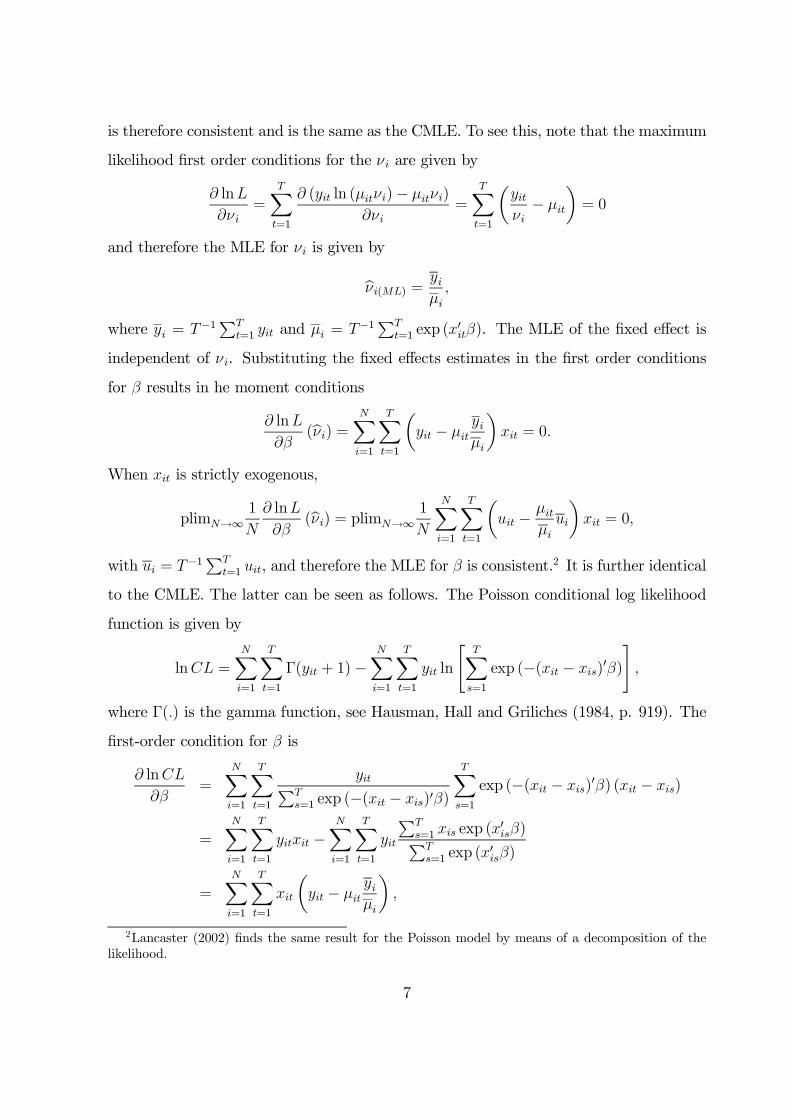
is therefore consistent and is the same as the CMLE. To see this, note that the maximum

likelihood first order conditions for the νi are given by

∂ lnL

∂νi=

TXt=1

∂ (yit ln (µitνi)− µitνi)

∂νi=

TXt=1

µyitνi− µit

¶= 0

and therefore the MLE for νi is given by

bνi(ML) =yiµi,

where yi = T−1PT

t=1 yit and µi = T−1PT

t=1 exp (x0itβ). The MLE of the fixed effect is

independent of νi. Substituting the fixed effects estimates in the first order conditions

for β results in he moment conditions

∂ lnL

∂β(bνi) = NX

i=1

TXt=1

µyit − µit

yiµi

¶xit = 0.

When xit is strictly exogenous,

plimN→∞1

N

∂ lnL

∂β(bνi) = plimN→∞

1

N

NXi=1

TXt=1

µuit − µit

µiui

¶xit = 0,

with ui = T−1PT

t=1 uit, and therefore the MLE for β is consistent.2 It is further identical

to the CMLE. The latter can be seen as follows. The Poisson conditional log likelihood

function is given by

lnCL =NXi=1

TXt=1

Γ(yit + 1)−NXi=1

TXt=1

yit ln

"TXs=1

exp (−(xit − xis)0β)

#,

where Γ(.) is the gamma function, see Hausman, Hall and Griliches (1984, p. 919). The

first-order condition for β is

∂ lnCL

∂β=

NXi=1

TXt=1

yitPTs=1 exp (−(xit − xis)0β)

TXs=1

exp (−(xit − xis)0β) (xit − xis)

=NXi=1

TXt=1

yitxit −NXi=1

TXt=1

yit

PTs=1 xis exp (x

0isβ)PT

s=1 exp (x0isβ)

=NXi=1

TXt=1

xit

µyit − µit

yiµi

¶,

2Lancaster (2002) finds the same result for the Poisson model by means of a decomposition of thelikelihood.

7

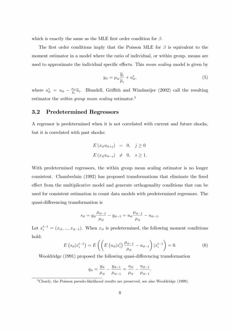
which is exactly the same as the MLE first order condition for β.

The first order conditions imply that the Poisson MLE for β is equivalent to the

moment estimator in a model where the ratio of individual, or within group, means are

used to approximate the individual specific effects. This mean scaling model is given by

yit = µityiµi+ u∗it, (5)

where u∗it = uit − µitµiui. Blundell, Griffith and Windmeijer (2002) call the resulting

estimator the within group mean scaling estimator.3

3.2 Predetermined Regressors

A regressor is predetermined when it is not correlated with current and future shocks,

but it is correlated with past shocks:

E (xituit+j) = 0, j ≥ 0E (xituit−s) 6= 0, s ≥ 1.

With predetermined regressors, the within group mean scaling estimator is no longer

consistent. Chamberlain (1992) has proposed transformations that eliminate the fixed

effect from the multiplicative model and generate orthogonality conditions that can be

used for consistent estimation in count data models with predetermined regressors. The

quasi-differencing transformation is

sit = yitµit−1µit− yit−1 = uit

µit−1µit− uit−1.

Let xt−1i = (xi1, ..., xit−1). When xit is predetermined, the following moment conditions

hold:

E¡sit|xt−1i

¢= E

µµE¡uit|xti

¢ µit−1µit− uit−1

¶|xt−1i

¶= 0. (6)

Wooldridge (1991) proposed the following quasi-differencing transformation

qit =yitµit− yit−1

µit−1=

uitµit− uit−1

µit−1,

3Clearly, the Poisson pseudo-likelihood results are preserved, see also Wooldridge (1999).

8

with moment conditions

E¡qit|xt−1i

¢= E

µµE (uit|xti)

µit− uit−1

µit−1

¶|xt−1i

¶= 0.

It is clear that a variable in xit can not have only non-positive or non-negative values,

as then the corresponding estimate for β is infinity. A way around this problem is to

transform xit in deviations from its overall mean, exit = xit−x, with x = 1NT

PNi=1

PTt=1 xit,

see Windmeijer (2000).

Both moment conditions can also be derived from a multiplicative model specification

yit = exp (x0itβ + ηi)wit = µitνiwit,

where xit is now predetermined w.r.t. wit. Again, we assume that the wit are not

serially correlated and not correlated with νi, and E (wit) = 1. The Chamberlain quasi-

differencing transformation in this case is equivalent to

sit = yitµit−1µit− yit−1 = νiµit−1 (wit − wit−1) ,

with moment conditions

E¡sit|xt−1i

¢= E

¡νiµit−1E

¡(wit − wit−1) |νi, xt−1i

¢ |xt−1i

¢= 0.

Equivalently, for the Wooldridge transformation,

qit =yitµit− yit−1

µit−1= νi (wit − wit−1)

and

E¡qit|xt−1i

¢= E

¡νiE

¡(wit − wit−1) |νi, xt−1i

¢ |xt−1i

¢= 0.

3.3 Endogenous Regressors

Regressors are endogenous when they are correlated with current (and possibly past)

shocks E (xituit−s) 6= 0, s ≥ 0, for the specification with additive errors uit, or when

E (xitwit−s) 6= 0, s ≥ 0, for the specification with multiplicative errors wit. It is clear from

the derivations in the previous section that we cannot find valid sequential conditional

9

moment conditions for the specification with additive errors due to the non-separability of

the uit and µit. For the multiplicative error specification, there is again non-separability

of µit−1 and (wit − wit−1) for the Chamberlain transformation and so

E¡sit|xt−2i

¢= E

¡νiµit−1E

¡(wit − wit−1) |νi, xt−1i

¢ |xt−2i

¢ 6= 0.In contrast, the Wooldridge transformation does not depend on µit or µit−1 in this case.

Valid moment conditions are then given by

E¡qit|xt−2i

¢= E

¡νiE

¡(wit − wit−1) |νi, xt−2i

¢ |xt−2i

¢= 0.

Therefore, in the case of endogenous explanatory variables, only the Wooldridge transfor-

mation can be used for the consistent estimation of the parameters β. This includes the

case of classical measurement error in xit, where the measurement error is not correlated

over time.

3.4 Dynamic Models

Specifying dynamic models for count data by including lags of the dependent count

variables in the explanatory part of the model is not as straightforward as with linear

models for a continuous dependent variable. Inclusion of the lagged dependent variable

in the exponential mean function may lead to rapidly exploding series. A better starting

point is to specify the model as in Crépon and Duguet (1997)

yit = h (yit−1, γ) exp (x0itβ + ηi) + uit,

where h (., .) > 0 is any given function describing the way past values of the dependent

variable are affecting the current value.

Let

dit = 1{yit=0},

then a possible choice for h (., .) is

h (yit, γ) = exp (γ1 ln (yit−1 + cdit−1) + γ2dit−1) ,

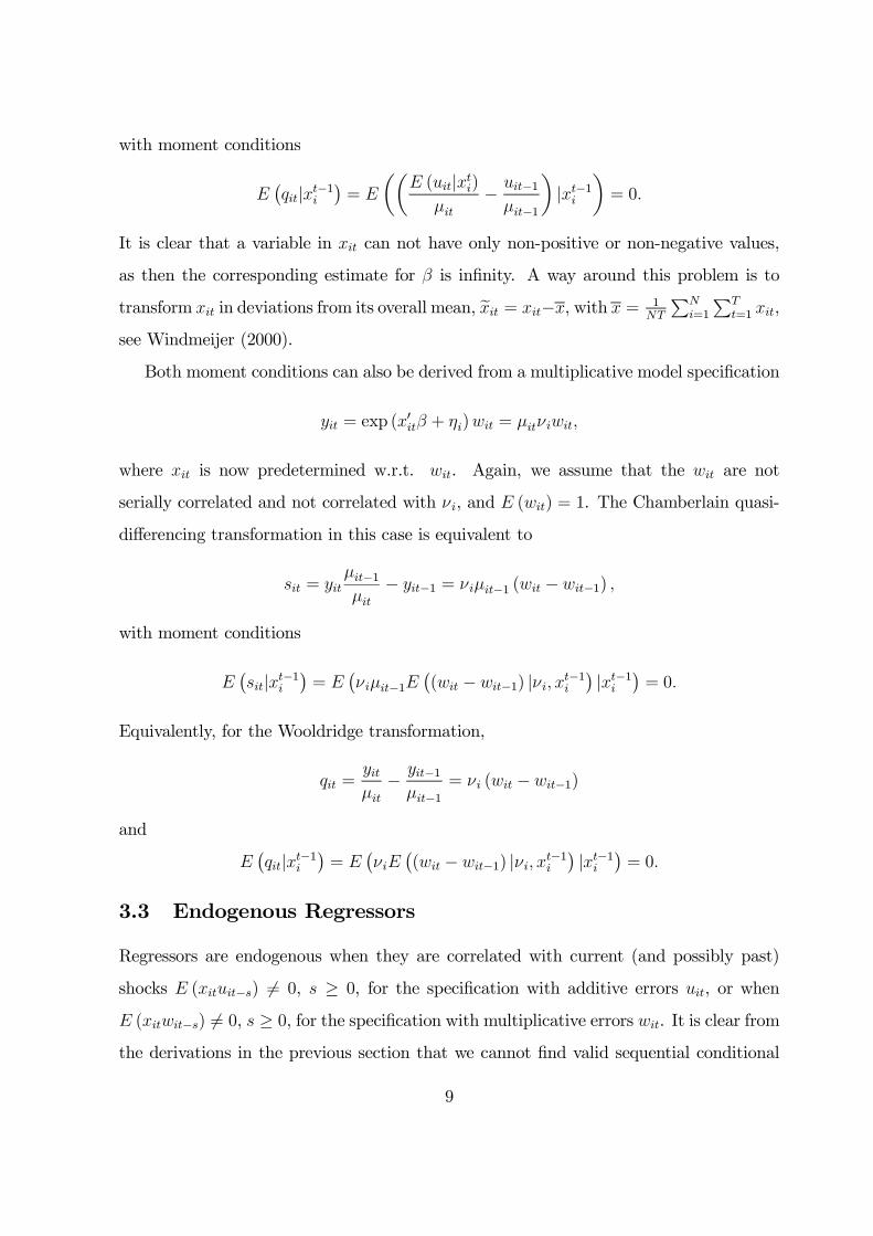
10

where c is a pre-specified constant. In this case, ln (yit−1) is included as a regressor for

positive yit−1, and zero values of yit−1 have a separate effect on current values of yit.

Crépon and Duguet (1997) considered

h (yit, γ) = exp (γ (1− dit−1)) ,

and extensions thereof to several regime indicators.

Blundell, Griffith and Windmeijer (2002) propose use of a linear feedback model for

modelling dynamic count panel data process. The linear feedback model of order 1

(LFM(1)) is defined as

yit = γyit−1 + exp(x0itβ + ηi) + uit

= γyit−1 + µitνi + uit,

where the lag of the dependent variable enters the model linearly. Extensions to in-

clude further lags are straightforward. The LFM has its origins in the Integer-Valued

Autoregressive (INAR) process and can be motivated as an entry-exit process with the

probability of exit equal to (1− γ). The correlation over time for the INAR(1) process

without additional regressors is similar to that of the AR(1) model, corr (yit, yit−j) = γj.

For the patents-R&D model, Blundell, Griffith and Windmeijer (2002) consider the

economic model

Pit = k³Rβit + (1− δ)Rβ

it−1 + (1− δ)2Rβit−2...

´νi + εit (7)

where Pit and Rit are the number of patents and R&D expenditures for firm i at time t

respectively, k is a positive constant and R&D expenditures depreciate geometrically at

rate δ. The long run steady state for firm i, ignoring feedback from patents to R&D, can

be written as

Pi =k

δRβi νi,

and β can therefore be interpreted as the long run elasticity. Inverting (7) leads to

Pit = kRβi νi + (1− δ)Pit−1 + uit

11

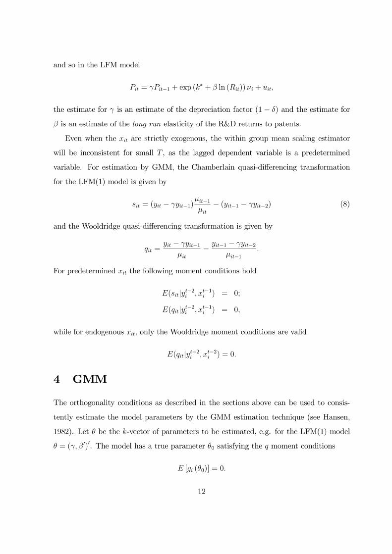
and so in the LFM model

Pit = γPit−1 + exp (k∗ + β ln (Rit)) νi + uit,

the estimate for γ is an estimate of the depreciation factor (1− δ) and the estimate for

β is an estimate of the long run elasticity of the R&D returns to patents.

Even when the xit are strictly exogenous, the within group mean scaling estimator

will be inconsistent for small T , as the lagged dependent variable is a predetermined

variable. For estimation by GMM, the Chamberlain quasi-differencing transformation

for the LFM(1) model is given by

sit = (yit − γyit−1)µit−1µit− (yit−1 − γyit−2) (8)

and the Wooldridge quasi-differencing transformation is given by

qit =yit − γyit−1

µit− yit−1 − γyit−2

µit−1.

For predetermined xit the following moment conditions hold

E(sit|yt−2i , xt−1i ) = 0;

E(qit|yt−2i , xt−1i ) = 0,

while for endogenous xit, only the Wooldridge moment conditions are valid

E(qit|yt−2i , xt−2i ) = 0.

4 GMM

The orthogonality conditions as described in the sections above can be used to consis-

tently estimate the model parameters by the GMM estimation technique (see Hansen,

1982). Let θ be the k-vector of parameters to be estimated, e.g. for the LFM(1) model

θ = (γ, β 0)0. The model has a true parameter θ0 satisfying the q moment conditions

E [gi (θ0)] = 0.

12

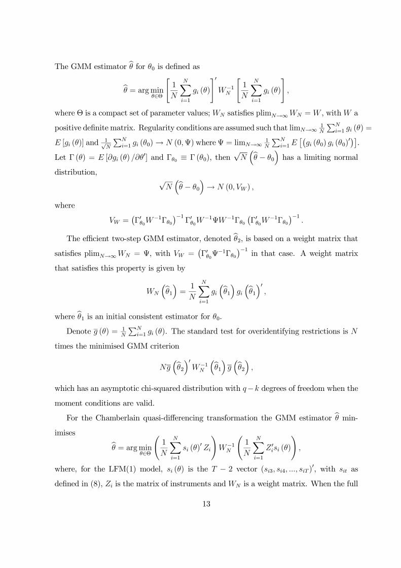
The GMM estimator bθ for θ0 is defined asbθ = argmin

θ∈Θ

"1

N

NXi=1

gi (θ)

#0W−1

N

"1

N

NXi=1

gi (θ)

#,

where Θ is a compact set of parameter values;WN satisfies plimN→∞WN = W , withW a

positive definite matrix. Regularity conditions are assumed such that limN→∞ 1N

PNi=1 gi (θ) =

E [gi (θ)] and 1√N

PNi=1 gi (θ0)→ N (0,Ψ)whereΨ = limN→∞ 1

N

PNi=1E

£¡gi (θ0) gi (θ0)

0¢¤.Let Γ (θ) = E [∂gi (θ) /∂θ

0] and Γθ0 ≡ Γ (θ0), then√N³bθ − θ0

´has a limiting normal

distribution,√N³bθ − θ0

´→ N (0, VW ) ,

where

VW =¡Γ0θ0W

−1Γθ0¢−1

Γ0θ0W−1ΨW−1Γθ0

¡Γ0θ0W

−1Γθ0¢−1

.

The efficient two-step GMM estimator, denoted bθ2, is based on a weight matrix thatsatisfies plimN→∞WN = Ψ, with VW =

¡Γ0θ0Ψ

−1Γθ0¢−1

in that case. A weight matrix

that satisfies this property is given by

WN

³bθ1´ = 1

N

NXi=1

gi³bθ1´ gi ³bθ1´0 ,

where bθ1 is an initial consistent estimator for θ0.Denote g (θ) = 1

N

PNi=1 gi (θ). The standard test for overidentifying restrictions is N

times the minimised GMM criterion

Ng³bθ2´0W−1

N

³bθ1´ g ³bθ2´ ,which has an asymptotic chi-squared distribution with q−k degrees of freedom when themoment conditions are valid.

For the Chamberlain quasi-differencing transformation the GMM estimator bθ min-imises bθ = argmin

θ∈Θ

Ã1

N

NXi=1

si (θ)0 Zi

!W−1

N

Ã1

N

NXi=1

Z 0isi (θ)

!,

where, for the LFM(1) model, si (θ) is the T − 2 vector (si3, si4, ..., siT )0, with sit as

defined in (8), Zi is the matrix of instruments andWN is a weight matrix. When the full

13

sequential set of instruments is used and xit is predetermined, the instrument matrix for

the LFM(1) model is given by

Zi =

yi1 xi1 xi2. . .

yi1 · · · yiT−2 xi1 · · · xiT−1

.The efficient weight matrix is

WN

³bθ1´ = 1

N

NXi=1

Z 0isi(bθ1)si(bθ1)0Zi,

where bθ1 can be a GMM estimator using for example WN =1N

PNi=1 Z

0iZi as the initial

weight matrix. As stated above, under the assumed regularity conditions both bθ1 and bθ2are asymptotically normally distributed. The asymptotic variance of bθ1 is estimated by

cvar³bθ1´ =1

N

µC³bθ1´0W−1

N C³bθ1´¶−1C ³bθ1´0W−1

N WN

³bθ1´W−1N C

³bθ1´×µC³bθ1´0W−1

N C³bθ1´¶−1

where

C³bθ1´ = 1

N

NXi=1

∂Z 0isi (θ)∂θ

|bθ1 .The asymptotic variance of the efficient two-step GMM, estimator is estimated by

cvar³bθ2´ = 1

N

µC³bθ2´0W−1

N

³bθ1´C ³bθ2´¶−1 .5 Applications and software

The instrumental variables methods for count data models with endogenous regressors

using cross section data, as described in Section 2, have often been applied in the health

econometrics literature. For example, Mullahy (1997) uses the multiplicative moment

conditions to estimate cigarette demand functions with a habit stock measure as en-

dogenous regressor. Windmeijer and Santos Silva (1997) estimate health care demand

functions with a self reported health measure as possible endogenous variable, while Vera-

Hernandez (1999) and Schellhorn (2001) estimate health care demand functions with

14

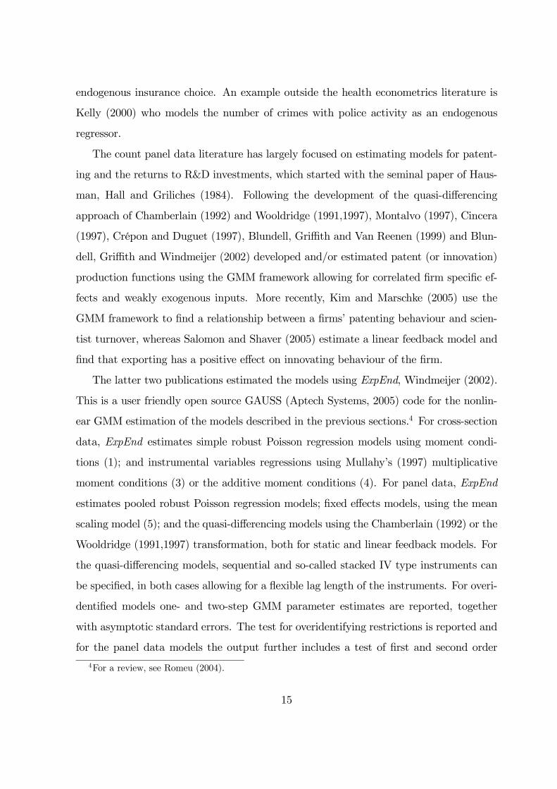
endogenous insurance choice. An example outside the health econometrics literature is

Kelly (2000) who models the number of crimes with police activity as an endogenous

regressor.

The count panel data literature has largely focused on estimating models for patent-

ing and the returns to R&D investments, which started with the seminal paper of Haus-

man, Hall and Griliches (1984). Following the development of the quasi-differencing

approach of Chamberlain (1992) and Wooldridge (1991,1997), Montalvo (1997), Cincera

(1997), Crépon and Duguet (1997), Blundell, Griffith and Van Reenen (1999) and Blun-

dell, Griffith and Windmeijer (2002) developed and/or estimated patent (or innovation)

production functions using the GMM framework allowing for correlated firm specific ef-

fects and weakly exogenous inputs. More recently, Kim and Marschke (2005) use the

GMM framework to find a relationship between a firms’ patenting behaviour and scien-

tist turnover, whereas Salomon and Shaver (2005) estimate a linear feedback model and

find that exporting has a positive effect on innovating behaviour of the firm.

The latter two publications estimated the models using ExpEnd, Windmeijer (2002).

This is a user friendly open source GAUSS (Aptech Systems, 2005) code for the nonlin-

ear GMM estimation of the models described in the previous sections.4 For cross-section

data, ExpEnd estimates simple robust Poisson regression models using moment condi-

tions (1); and instrumental variables regressions using Mullahy’s (1997) multiplicative

moment conditions (3) or the additive moment conditions (4). For panel data, ExpEnd

estimates pooled robust Poisson regression models; fixed effects models, using the mean

scaling model (5); and the quasi-differencing models using the Chamberlain (1992) or the

Wooldridge (1991,1997) transformation, both for static and linear feedback models. For

the quasi-differencing models, sequential and so-called stacked IV type instruments can

be specified, in both cases allowing for a flexible lag length of the instruments. For overi-

dentified models one- and two-step GMM parameter estimates are reported, together

with asymptotic standard errors. The test for overidentifying restrictions is reported and

for the panel data models the output further includes a test of first and second order

4For a review, see Romeu (2004).

15

serial correlation of the quasi-differencing "residuals" sit

³bθ´ or qit ³bθ´. If the model iscorrectly specified one expects to find an MA(1) serial correlation structure.

Another package that enables researchers to estimate these model types is TSP, Hall

and Cummins (2005). Kitazawa (2000) provides various TSP procedures for the estima-

tion of count panel data models. Also LIMDEP, Greene (2005), provides an environment

where these models can be estimated.

6 Finite sample inference

Standard Wald tests based on two-step efficient GMM estimators are known to have

poor finite sample properties (see e.g. Blundell and Bond (1998)). Bond and Windmei-

jer (2005) therefore analysed the finite sample performance of various alternative test

procedures for testing linear restrictions in linear panel data models. The statistics they

found to perform well in Monte Carlo exercises were an alternative two-step Wald test

that uses a finite sample correction for the asymptotic variance matrix, the LM test, and

a simple criterion-based test. In this section we briefly describe these procedures and

adapt them to the case of nonlinear GMM estimation where necessary.

Newey and Smith (2004) have shown that the GMM estimator can further also suffer

from quite large finite sample biases and advocate use of Generalized Empirical Likelihood

(GEL) estimators that they show to have smaller finite sample biases. We will consider

here the performance of the Continuous Updating Estimator (CUE) as proposed by

Hansen, Heaton and Yaron (1996), which is a GEL estimator. The Wald test based on

the CUE has also been shown to perform poorly in finite samples by e.g. Hansen, Heaton

and Yaron (1996). Newey and Windmeijer (2005) derive the asymptotic distribution of

the CUE when there are many weak moment conditions. The asymptotic variance in

this case is larger than the usual asymptotic one and we will analyse the performance

of an alternative Wald test that uses an estimate for this larger asymptotic variance,

together with a criterion based test for the CUE as proposed by Hansen, Heaton and

Yaron (1996).

16

The estimators and test procedures will be evaluated in a Monte Carlo study of

testing linear restrictions in a static count panel data model with an explanatory variable

that is correlated with the fixed unobserved heterogeneity and which is predetermined.

The Chamberlain quasi-differencing transformation will be used with sequential moment

conditions.

6.1 Wald test and finite sample variance correction

The standard Wald test for testing r linear restrictions of the form r (θ0) = 0 is calculated

as

Wald = r³bθ´0 ³R0cvar³bθ´R´−1 r ³bθ´ ,

where R = ∂r (θ) /∂θ0, and has an asymptotic χ2r distribution under the null. Based on

the two-step GMM estimator and using its conventional asymptotic variance estimate, the

Wald test has often been found to overreject correct null hypotheses severely compared to

its nominal size. This can occur even when the estimator has negligible finite sample bias,

due to the fact that the estimated asymptotic standard errors can be severely downward

biased in small samples. Windmeijer (2005) proposed a finite sample variance correction

that takes account of the extra variation due to the presence of the estimated parametersbθ1 in the weight matrix. He showed by means of a Monte Carlo study that this correctionworks well in linear models, but it is not clear how well it will work in nonlinear GMM.

To derive the finite sample corrected variance, let

g (θ) =1

N

NXi=1

gi (θ) ; C (θ) =∂g (θ)

∂θ0; G (θ) =

∂C (θ)

∂θ,

and

bθ0,WN=

1

2

∂QWN

∂θ|θ0 = C (θ0)

0W−1N g (θ0) ;

Aθ0,WN=

1

2

∂2QWN

∂θ∂θ0|θ0 = C (θ0)

0W−1N C (θ0) +G (θ0)

0 ¡Ik ⊗W−1N g (θ0)

¢.

A standard first order Taylor series approximation of bθ2 around θ0, conditional on

WN

³bθ1´, results inbθ2 − θ0 = −A−1θ0,WN(bθ1)bθ0,WN(bθ1) +Op

¡N−1¢ .

17

A further expansion of bθ1 around θ0 results in

bθ2 − θ0 = −A−1θ0,WN (θ0)bθ0,WN (θ0) +Dθ0,WN (θ0)

³bθ1 − θ0

´+Op

¡N−1¢ , (9)

where

WN (θ0) =1

N

NXi=1

gi (θ0) gi (θ0)0

and

Dθ0,WN (θ0) =∂

∂θ0³−A−1θ0,WN (θ)

bθ0,WN (θ)

´|θ0

is a k × k matrix.

Let bθ1 be a one-step GMM estimator that uses a weight matrix WN that does not

depend on estimated parameters. An estimate of the variance of bθ2 that incorporates theterm involving the one-step parameter estimates used in the weight matrix can then be

obtained as

cvarc ³bθ2´ =1

NA−1bθ2,WN(bθ1)C

³bθ2´0W−1N

³bθ1´C ³bθ2´A−1bθ2,WN(bθ1)+1

NDbθ2,WN(bθ1)A−1bθ1,WN

C³bθ1´0W−1

N C³bθ2´A−1bθ2,WN(bθ1)

+1

NA−1bθ2,WN(bθ1)C

³bθ2´0W−1N C

³bθ1´A−1bθ1,WND0bθ2,WN(bθ1)

+ Dbθ2,WN(bθ1)cvar³bθ1´D0bθ2,WN(bθ1),where the jth column of Dbθ2,WN(bθ1) is given by

Dbθ2,WN(bθ1)[., j] = A−1bθ2,WN(bθ1)C³bθ2´0W−1

N

³bθ1´ ∂WN (θ)

∂θj|bθ2W−1

N

³bθ1´ g ³bθ2´ ,and

∂WN (θ)

∂θj=1

N

NXi=1

µ∂gi (θ)

∂θjgi (θ)

0 + gi (θ)∂gi (θ)

0

∂θj

¶.

The alternative two-step Wald test that uses a finite sample correction for the asymptotic

variance matrix is then defined as

Waldc = r³bθ2´0 ³R0cvarc ³bθ2´R´−1 r ³bθ2´ .

18

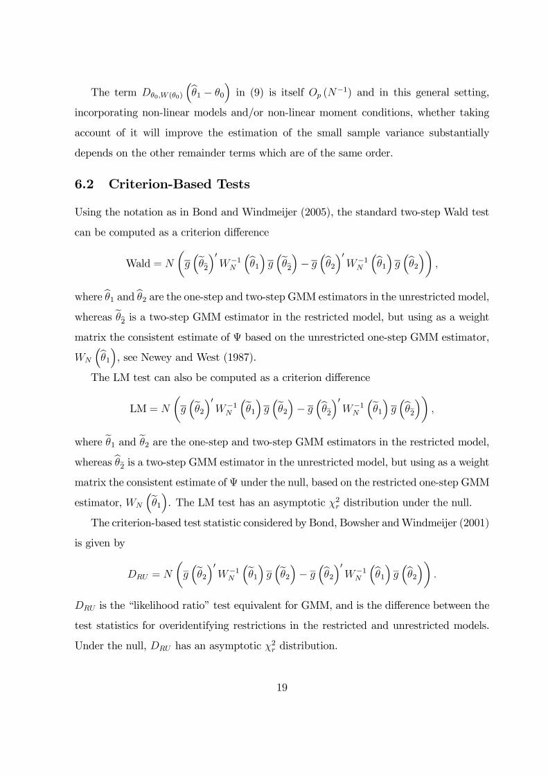
The term Dθ0,W (θ0)

³bθ1 − θ0

´in (9) is itself Op (N

−1) and in this general setting,

incorporating non-linear models and/or non-linear moment conditions, whether taking

account of it will improve the estimation of the small sample variance substantially

depends on the other remainder terms which are of the same order.

6.2 Criterion-Based Tests

Using the notation as in Bond and Windmeijer (2005), the standard two-step Wald test

can be computed as a criterion difference

Wald = N

µg³eθb2´0W−1

N

³bθ1´ g ³eθb2´− g³bθ2´0W−1

N

³bθ1´ g ³bθ2´¶ ,

where bθ1 and bθ2 are the one-step and two-step GMM estimators in the unrestricted model,

whereas eθb2 is a two-step GMM estimator in the restricted model, but using as a weight

matrix the consistent estimate of Ψ based on the unrestricted one-step GMM estimator,

WN

³bθ1´, see Newey and West (1987).The LM test can also be computed as a criterion difference

LM = N

µg³eθ2´0W−1

N

³eθ1´ g ³eθ2´− g³bθe2´0W−1

N

³eθ1´ g ³bθe2´¶ ,

where eθ1 and eθ2 are the one-step and two-step GMM estimators in the restricted model,

whereas bθe2 is a two-step GMM estimator in the unrestricted model, but using as a weight

matrix the consistent estimate of Ψ under the null, based on the restricted one-step GMM

estimator, WN

³eθ1´. The LM test has an asymptotic χ2r distribution under the null.

The criterion-based test statistic considered by Bond, Bowsher andWindmeijer (2001)

is given by

DRU = N

µg³eθ2´0W−1

N

³eθ1´ g ³eθ2´− g³bθ2´0W−1

N

³bθ1´ g ³bθ2´¶ .

DRU is the “likelihood ratio” test equivalent for GMM, and is the difference between the

test statistics for overidentifying restrictions in the restricted and unrestricted models.

Under the null, DRU has an asymptotic χ2r distribution.

19

6.3 Continuous Updating Estimator

The Continuous Updating Estimator (CUE) is given by

bθCU = argminθ∈Θ

Q (θ) ;

Q (θ) =1

2g (θ)0W−1

N (θ) g (θ) ,

where, as before,

WN (θ) =1

N

NXi=1

gi (θ) gi (θ)0

and so the CUE minimises the criterion function including the parameters in the weight

matrix. The limiting distribution under standard regularity conditions is given by

√N³bθCU − θ0

´→ N (0, V ) ; V =

¡Γ0θ0Ψ

−1Γθ0¢−1

and is the same as the efficient two-step GMM estimator. The asymptotic variance of

the CUE is computed as

cvar³bθCU´ = 1

N

µC³bθCU´0W−1

N

³bθCU´C ³bθCU´¶−1 ,which is used in the calculation of the standard Wald test. Again, it has been shown by

e.g. Hansen, Heaton and Yaron (1996) that the asymptotic standard errors are severely

downward biased, leading to overrejection of a true null hypothesis using the Wald test.

Newey and Windmeijer (2005) derive the asymptotic distribution of the CUE under

many weak instrument asymptotics. In these asymptotics, the number of instruments

is allowed to grow with the sample size N , with the increase in number of instruments

accompanied by an increase in the concentration parameter. The resulting limiting dis-

tribution of the CUE is again the normal distribution, but convergence is at a slower rate

than√N . The asymptotic variance is in this case larger than the asymptotic variance

using conventional asymptotics, and can be estimated consistently by

cvar³bθCU´c=1

NH−1

³bθCU´S ³bθCU´0W−1N

³bθCU´S ³bθCU´H−1³bθCU´ ,

20

where

H (θ) =∂2Q (θ)

∂θ∂θ0; S (θ) = (S1 (θ) , S2 (θ) , ..., Sk (θ))

Sj (θ) =

µ∂g (θ)

∂θj− Λj (θ)W

−1N (θ) g (θ)

¶Λj (θ) =

1

N

NXi=1

∂gi (θ)

∂θjgi (θ)

0 .

Here, unlike the usual asymptotics, the middle matrix S³bθCU´0W−1

N

³bθCU´S ³bθCU´estimates a different, larger object than the Hessian. Also, the use of the Hessian is im-

portant, as the more common formula C³bθCU´0W−1

N

³bθCU´C ³bθCU´ has extra randomterms that are eliminated in the Hessian under the alternative asymptotics.

Hansen, Heaton and Yaron (1996) proposed the use of a criterion-based test similar

to DRU , but based on the CUE. Their test statistic DCURU is defined as

DCURU = 2N

³Q³eθCU´−Q

³bθCU´´ ,where bθCU and eθCU are the CUEs for the unrestricted and restricted models respectively.Under the null, DCU

RU has an asymptotic χ2r distribution.

6.4 Monte Carlo results

In this section we will illustrate the finite sample performance of the GMM estimators

and the test statistics as discussed in the previous sections by means of a small Monte

Carlo study. The data generating process is given by

yit ∼ Poisson (exp (xitβ + ηi + εit))

xit = ρxit−1 + δηi + θεit−1 + ωit

ηi ∼ N¡0, σ2η

¢; εit ∼ N

¡0, σ2ε

¢; ωit ∼ N

¡0, σ2ω

¢,

β = 0.5; δ = 0.1; θ = 0.3; σ2η = 0.3; σ2ε = 0.3; σ

2ω = 0.25

ρ = {0.5, 0.8} .

The dependent variable is a count variable, generated from the Poisson distribution with

unobserved fixed normally distributed heterogeneity ηi and further idiosyncratic normally

21

distributed heterogeneity εit. The xit are correlated with the ηi and εit−1 and are therefore

predetermined.

Table 1 presents estimation results from 10, 000 Monte Carlo replications for the one-

and two-step GMM estimators as well as the continuous updating estimator for T = 6,

N = 250 and ρ = 0.5 or ρ = 0.8, using the moment conditions (6) as proposed by

Chamberlain (1992). The instruments set is given by

Zi =

xi1

xi1 xi2. . .

xi1 · · · xiT−1

and hence there are a total of 15 moment conditions.The one-step GMM estimator uses

WN =1N

PNi=1 Z

0iZi as the weight matrix.

When ρ = 0.5, the instruments are quite strong. The one-step GMM estimator,

denoted GMM1 in the table, has a moderate downward bias of −0.0408. Its standarddeviation is 0.1053, which seems well approximated by the asymptotic standard error.

The mean of the estimated standard errors is equal to 0.1031. The two-step GMM

estimator, denoted GMM2, has a smaller bias of−0.0211 and a smaller standard deviationof 0.0803, representing a substantial efficiency gain with more than a 23% reduction

in standard deviation. In contrast to the one-step estimator, the mean of the usual

asymptotic standard errors is 19% smaller than the standard deviation. However, taking

account of the extra variation due to the presence of the one-step estimates in the weight

matrix results in finite sample corrected standard errors with a mean of 0.0799, which is

virtually identical to the standard deviation. The CUE has a very small bias of 0.0043,

with a standard deviation of 0.0904, which is larger than that of the two-step GMM

estimator, but smaller than that of the one-step estimator. The mean of the usual

asymptotic standard errors is exactly the same as that of the two-step GMM estimator

and in this case it is almost 28% smaller than the standard deviation. The standard

errors resulting from the many weak instruments asymptotics have a mean of 0.0918,

which is virtually the same as the standard deviation.

22

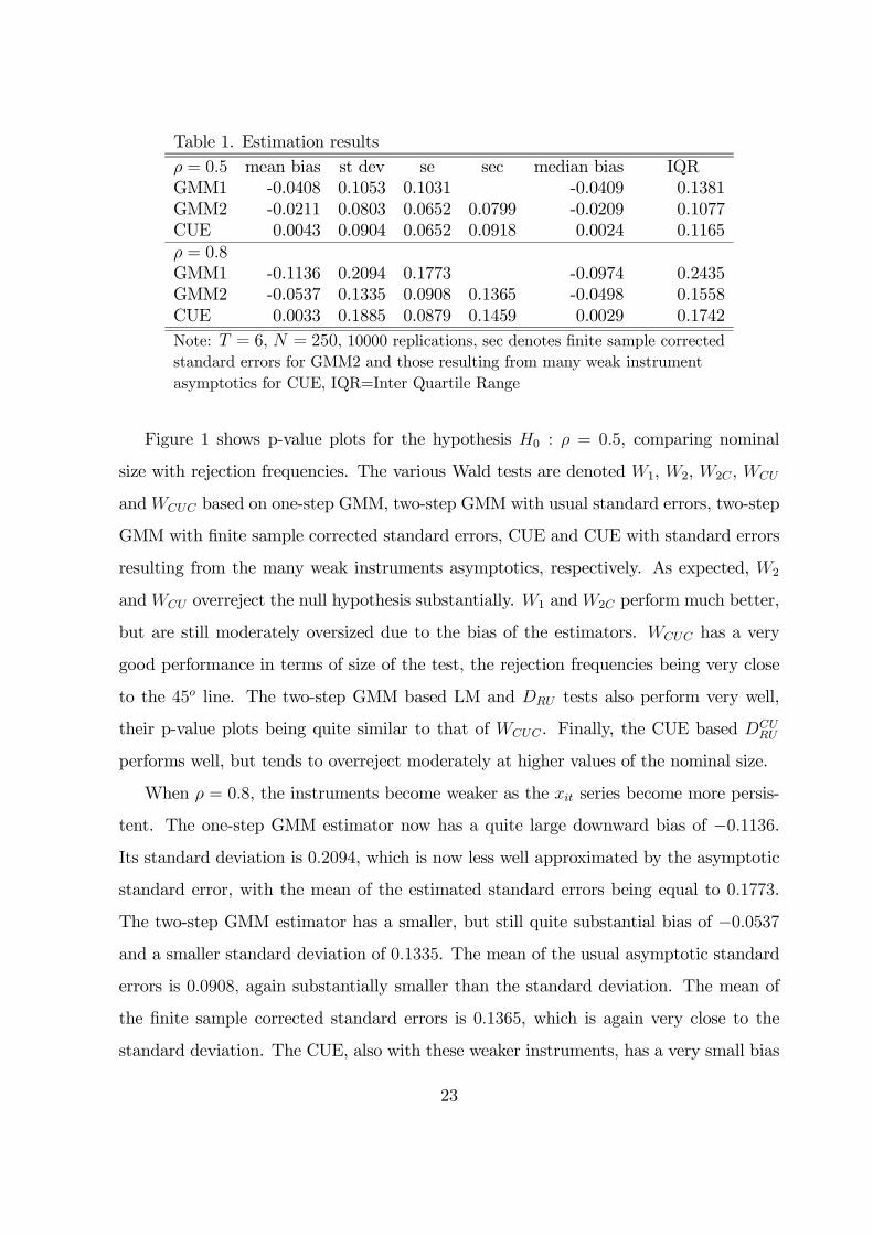
Table 1. Estimation resultsρ = 0.5 mean bias st dev se sec median bias IQRGMM1 -0.0408 0.1053 0.1031 -0.0409 0.1381GMM2 -0.0211 0.0803 0.0652 0.0799 -0.0209 0.1077CUE 0.0043 0.0904 0.0652 0.0918 0.0024 0.1165ρ = 0.8GMM1 -0.1136 0.2094 0.1773 -0.0974 0.2435GMM2 -0.0537 0.1335 0.0908 0.1365 -0.0498 0.1558CUE 0.0033 0.1885 0.0879 0.1459 0.0029 0.1742Note: T = 6, N = 250, 10000 replications, sec denotes finite sample correctedstandard errors for GMM2 and those resulting from many weak instrumentasymptotics for CUE, IQR=Inter Quartile Range

Figure 1 shows p-value plots for the hypothesis H0 : ρ = 0.5, comparing nominal

size with rejection frequencies. The various Wald tests are denoted W1, W2, W2C , WCU

andWCUC based on one-step GMM, two-step GMM with usual standard errors, two-step

GMM with finite sample corrected standard errors, CUE and CUE with standard errors

resulting from the many weak instruments asymptotics, respectively. As expected, W2

andWCU overreject the null hypothesis substantially. W1 andW2C perform much better,

but are still moderately oversized due to the bias of the estimators. WCUC has a very

good performance in terms of size of the test, the rejection frequencies being very close

to the 45o line. The two-step GMM based LM and DRU tests also perform very well,

their p-value plots being quite similar to that of WCUC . Finally, the CUE based DCURU

performs well, but tends to overreject moderately at higher values of the nominal size.

When ρ = 0.8, the instruments become weaker as the xit series become more persis-

tent. The one-step GMM estimator now has a quite large downward bias of −0.1136.Its standard deviation is 0.2094, which is now less well approximated by the asymptotic

standard error, with the mean of the estimated standard errors being equal to 0.1773.

The two-step GMM estimator has a smaller, but still quite substantial bias of −0.0537and a smaller standard deviation of 0.1335. The mean of the usual asymptotic standard

errors is 0.0908, again substantially smaller than the standard deviation. The mean of

the finite sample corrected standard errors is 0.1365, which is again very close to the

standard deviation. The CUE, also with these weaker instruments, has a very small bias

23

Figure 1. P-value plot, H0 : ρ = 0.5

of 0.0033, with a standard deviation of 0.1885. In this case the so-called no moment-

problem starts to become an issue for the CUE, though, with some outlying estimates

inflating the standard deviation, see Guggenberger (2005). It is therefore better to look

at the median bias and inter quartile range (IQR) in this case, which shows that the CUE

is median unbiased with an IQR which is only slightly larger than that of the two-step

GMM estimator, 0.1742 versus 0.1558 respectively.

Figure 2 shows p-value plots for the hypothesis H0 : ρ = 0.8. W2 and WCU overre-

ject the null hypothesis even more than when ρ = 0.5. W1 performs better, but is still

substantially oversized. W2C and WCUC perform quite well and quite similar, slightly

overrejecting the null. The two-step GMM based LM and DRU are again the best per-

formers in terms of size, whereas the CUE based DCURU performs worse than W2C and

WCUC .

24

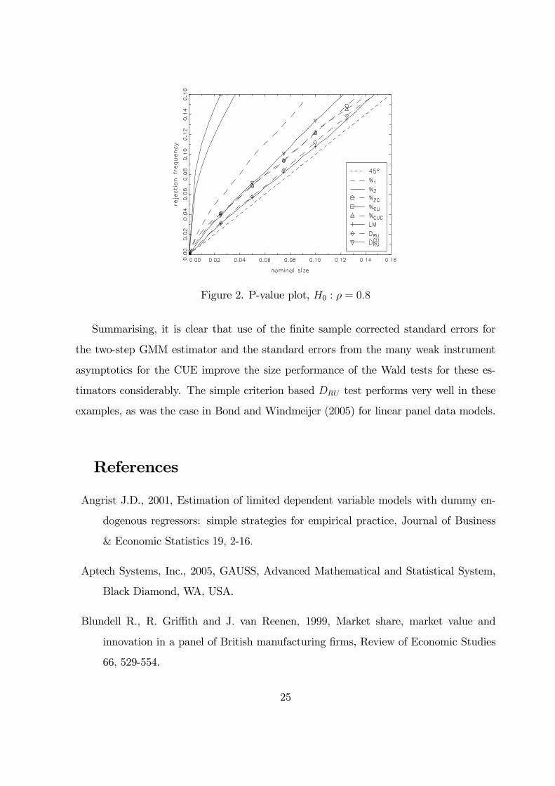
Figure 2. P-value plot, H0 : ρ = 0.8

Summarising, it is clear that use of the finite sample corrected standard errors for

the two-step GMM estimator and the standard errors from the many weak instrument

asymptotics for the CUE improve the size performance of the Wald tests for these es-

timators considerably. The simple criterion based DRU test performs very well in these

examples, as was the case in Bond and Windmeijer (2005) for linear panel data models.

References

Angrist J.D., 2001, Estimation of limited dependent variable models with dummy en-

dogenous regressors: simple strategies for empirical practice, Journal of Business

& Economic Statistics 19, 2-16.

Aptech Systems, Inc., 2005, GAUSS, Advanced Mathematical and Statistical System,

Black Diamond, WA, USA.

Blundell R., R. Griffith and J. van Reenen, 1999, Market share, market value and

innovation in a panel of British manufacturing firms, Review of Economic Studies

66, 529-554.

25

Blundell R., R. Griffith and F. Windmeijer, 2002, Individual effects and dynamics in

count data models, Journal of Econometrics 108, 113-131.

Bond S.R., C. Bowsher and F. Windmeijer, 2001, Criterion-Based inference for GMM

in autoregressive panel data models, Economics Letters 73, 379-388.

Bond S.R. and F. Windmeijer, 2005, Reliable inference for GMM estimators? Finite

sample procedures in linear panel data models, Econometric Reviews 24, 1-37.

Chamberlain G., 1992, Comment: Sequential moment restrictions in panel data, Journal

of Business & Economic Statistics 10, 20-26.

Cincera M., 1997, Patents, R&D, and technological spillovers at the firm level: some

evidence from econometric count models for panel data, Journal of Applied Econo-

metrics 12, 265-280.

Crépon B. and E. Duguet, 1997, Estimating the innovation function from patent num-

bers: GMM on count panel data, Journal of Applied Econometrics 12, 243-263.

Greene, W.H., 2005, LIMDEP 8.0, Econometric Software, Inc., Plainview, NY, USA.

Guggenberger P., 2005, Monte-carlo evidence suggesting a no moment problem of the

continuous updating estimator, Economics Bulletin 3, 1-6.

Hall B. and C. Cummins, 2005, TSP 5.0, TSP International, Palo Alto, CA, USA.

Hansen L.P., 1982, Large sample properties of generalized method of moments estima-

tors, Econometrica 50, 1029-1054.

Hansen L.P., J. Heaton and A. Yaron, 1996, Finite-sample properties of some alternative

GMM estimators, Journal of Business & Economic Statistics 14, 262-280.

Hausman J., B. Hall and Z. Griliches, 1984, Econometric models for count data and an

application to the patents-R&D relationship, Econometrica 52, 909-938.

26

Kelly M., 2000, Inequality and crime, The Review of Economics and Statistics 82, 530-

539.

Kitazawa Y., 2000, TSP procedures for count panel data estimation, Kyushu Sangyo

University.

Lancaster T., 2002, Orthogonal parameters and panel data, Review of Economic Studies

69, 647-666.

Kim J. and G. Marschke, 2005, Labor mobility of scientists, technological diffusion and

the firm’s patenting decision, The RAND Journal of Economics 36, 298-317.

Manning W.G., A. Basu and J. Mullahy, 2005, Generalized modeling approaches to risk

adjustment of skewed outcomes data, Journal of Health Economics 24, 465-488.

Montalvo J.G., 1997, GMM estimation of count-panel-data models with fixed effects

and predetermined instruments, Journal of Business and Economic Statistics 15,

82-89.

Mullahy J., 1997, Instrumental variable estimation of Poisson regression models: appli-

cation to models of cigarette smoking behavior, Review of Economics and Statistics

79, 586-593.

Newey W.K. and R.J. Smith, 2004, Higher order properties of GMM and generalized

empirical likelihood estimators, Econometrica 72, 219-255.

Newey W.K. and K.D. West, 1987, Hypothesis testing with efficient method of moments

estimation, International Economic Review 28, 777-787.

Newey W.K. and F. Windmeijer, 2005, GMM with many weak moment conditions,

cemmap Working Paper No CWP18/05.

Romeu A., 2004, ExpEnd : Gauss code for panel count data models, Journal of Applied

Econometrics 19, 429-434.

27

Salomon R.M. and J.M. Shaver, 2005, Learning by exporting: new insights from exam-

ining firm innovation, Journal of Economics and Management Strategy 14, 431-460.

Santos Silva J.M.C. and S. Tenreyro, 2006, The log of gravity, The Review of Economics

and Statistics 88.

Schellhorn M., 2001, The effect of variable health insurance deductibles on the demand

for physician visits, Health Economics 10, 441-456.

Vera-Hernandez, A.M., 1999, Duplicate coverage and demand for health care. The case

of Catalonia, Health Economics 8, 579-598.

Windmeijer F., 2000, Moment conditions for fixed effects count data models with en-

dogenous regressors, Economics Letters 68, 21-24.

Windmeijer F., 2002, ExpEnd, a Gauss programme for non-linear GMM estimation of

exponential models with endogenous regressors for cross section and panel data,

cemmap Working Paper No. CWP14/02.

Windmeijer F., 2005, A finite sample correction for the variance of linear efficient two-

step GMM estimators, Journal of Econometrics 126, 25-517.

Windmeijer F. and J.M.C. Santos Silva, 1997, Endogeneity in count data models: an

application to demand for health care, Journal of Applied Econometrics 12, 281-

294.

Wooldridge J.M., 1991, Multiplicative panel data models without the strict exogeneity

assumption, MIT Working Paper No. 574.

Wooldridge J.M., 1997, Multiplicative panel data models without the strict exogeneity

assumption, Econometric Theory 13, 667-678.

Wooldridge J.M., 1999, Distribution-free estimation of some nonlinear panel data mod-

els, Journal of Econometrics 90, 77-97.

28