GloPel User Manual - radicals.uni-freiburg.de

GloPel User Manual

Version 1.0.1

GloPel

by

Stephan Rein

[email protected]

https://www.radicals.uni-freiburg.de/de/software

mailto:[email protected]

https://www.radicals.uni-freiburg.de/de/software

Contents

1 Introduction 4

1.1 Installation Instructions . . . . . . . . . . . . . . . . . . . . . . . . . . . . 6

1.1.1 Run from source . . . . . . . . . . . . . . . . . . . . . . . . . . . . 6

1.1.2 Use compiled executables . . . . . . . . . . . . . . . . . . . . . . . . 6

2 Using GloPel 8

2.1 Loading data . . . . . . . . . . . . . . . . . . . . . . . . . . . . . . . . . . 8

2.2 Data (pre)-processing . . . . . . . . . . . . . . . . . . . . . . . . . . . . . . 9

2.2.1 Phase correction . . . . . . . . . . . . . . . . . . . . . . . . . . . . 10

2.2.2 Normalization and zero-time . . . . . . . . . . . . . . . . . . . . . . 10

2.2.3 Background correction . . . . . . . . . . . . . . . . . . . . . . . . . 11

2.3 Analysis . . . . . . . . . . . . . . . . . . . . . . . . . . . . . . . . . . . . . 12

2.3.1 Analysis using Tikhonov regularization . . . . . . . . . . . . . . . . 13

2.3.2 Model-based fitting . . . . . . . . . . . . . . . . . . . . . . . . . . . 16

2.4 Inspection and Validation . . . . . . . . . . . . . . . . . . . . . . . . . . . 19

2.5 Validation . . . . . . . . . . . . . . . . . . . . . . . . . . . . . . . . . . . . 19

2.6 Save the results . . . . . . . . . . . . . . . . . . . . . . . . . . . . . . . . . 21

3 Global analysis 23

3.1 Data processing of two time traces . . . . . . . . . . . . . . . . . . . . . . 23

3.2 Global analysis of two time traces . . . . . . . . . . . . . . . . . . . . . . . 24

2

Preface

GloPel has been developed in the group of Prof. Dr. Stefan Weber at the University of

Freiburg, Freiburg im Breisgau, Germany, during the last couple of years as a software

for advanced global analysis of PELDOR/DEER spectra.

This manual describes the general usage of GloPel and gives an overview of the maths

behind that has been implemented.

If you use GloPel for your own research and publish results accordingly, please give credits

citing the appropriate reference :

Stephan Rein, Philipp Lewe, Susana L. Andrade, Sylwia Kacprzak, and Stefan

Weber. Global analysis of complex PELDOR time traces. Journal of Magnetic

Resonance, 295 (2018) 17–26

Some parts of this Manual were taken form the publication [1] of which the author was

responsible for program development and for writing most parts of the manuscript.

A number of people have helped shaping GloPel and the ideas behind. First and foremost,

Prof. Dr. Stefan Weber and Dr. Sylwia Kacprzak (now Bruker Biospin) were for years the

driving force behind GloPel due to the need for advanced analysis of PELDOR/DEER data

with limited signal-to-noise ratio. Dr. Till Biskup (now Saarland University) contributed

ideas for programming and details of the implementation that make all the difference

between a program useful for a larger audience and a simple in-house solution.

Freiburg, October 2019

Stephan Rein

Disclaimer

GloPel is distributed under a GPLv3 license. The software is provided ”as is”, without

warranty of any kind, express or implied, including but not limited to the warranties of

merchantability, fitness for a particular purpose and noninfringement.

3

1 Introduction

GloPel is a platform-independent GUI application, designed for advanced and global anal-

ysis that can reliably analyze PELDOR data from samples that cannot be measured

with high signal-to-noise ratio in sufficiently long observation time windows. The here-

presented global-analysis approach employs Tikhonov regularization of the solution to the

inverse problem. Alternatively, a model-based (sum of multiple Gaussian functions) fit

may be used.

GloPel is currently restricted to the global analysis of two time traces, for the sake of

keeping the GUI as simple as possible. It is recommended to acquire two experimental

time traces, one with a longer acquisition time and a poorer signal-to-noise ratio and one

with a short acquisition time and a good signal-to-noise ration. It is highly recommended

to keep all spectrometer settings constant and only change the acquisition time and PEL-

DOR step size. Especially taking the sample out between the two experiments should be

avoided. The standard procedure in GloPel, explained in detail in the following sections,

for a single analysis are:

1. Loading the raw experimental data set (as .txt or BES3T Bruker file format)

2. Preprocessing of the raw data (settings for background function, background dimen-

sion, cutting of data, ...)

3. Analysis of the data with either Tikhonov regularization or multi-Gaussian fitting

4. Checking the results on the Residual Inspection submodule

5. Validation of the results (in the case of Tikhonov regularization) using the Validation

submodule

6. Saving all the analysis results

For a global analysis the steps are:

4

1. Analysis of data set 1 (the PELDOR time time trace with longer acquisition time)

2. Loading data set 2

3. Data preprocessing of data set 2 using the background function of data set 1

4. Analysis of data set 2

5. Global analysis of both data sets

6. Residual inspection and validation of the results (in case of global Tikhonov regu-

larization)

7. Saving the global analysis results (the analysis of the individual analysis is saved

automatically)

For details of the individual steps and installation details, read the following sections.

5

1.1 Installation Instructions

GloPel is available free of charge and open source (see license). We recommend everybody

with a recent Python installation on their computers to download the source code via pip

and use it. In this case, no real installation is necessary, and starting GloPel is as simple

as typing the following command into a terminal:

1.1.1 Run from source

Install GloPel in a Python3 environment

pip install glopel

Once installed, the program can be started by just calling GloPel from the console by just

giving:

glopel

If you want to use it withing a python script/console give:

python3

>>> from GloPel.GloPel import run

>>> run()

1.1.2 Use compiled executables

However, GloPel can be downloaded as executable binary for Windows and several Linux

flavors. It was tested on various systems including Windows 7 (32-bit and 64-bit archi-

tecture), Windows 10 (32-bit and 64-bit architecture), and Ubuntu 16.04.

Please note that these versions are much harder to debug if something goes wrong, there-

fore, they are provided as is without any further support.

A note on how these binaries have been created: Thanks to PyInstaller, it is rather

straightforward to create binary distributions of Python programs, both as directories

6

with all the necessary files contained as well as single-file executables. PyInstaller allows

to define additional options in a “spec” file. This file is included in the sources available.

To get a one-file binary, it was called simply as follows:

pyinstaller --onefile --noconsole GloPel.spec

1. Binaries for Linux have been built with Ubuntu 16.04 (Xenial Xerus) and a Python

installation consisting of Python 3.5, matplotlib 3.0.2, PyQt 5.11.3, NumPy 1.16.1,

SciPy 1.2.0, reportlab 3.5.19, cvxopt 1.2.3, osqp 0.6.1

2. Binaries for Windows have been built with Windows7 (32-bit architecture) and a

Python installation consisting of Python 3.5 or, matplotlib 3.0.2, NumPy (+MKL)

1.11.3, SciPy 1.2.0, PyQt 5.11.3, osqp 0.6.1

7

2 Using GloPel

2.1 Loading data

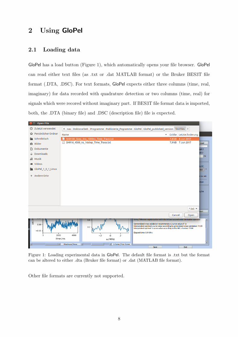
GloPel has a load button (Figure 1), which automatically opens your file browser. GloPel

can read either text files (as .txt or .dat MATLAB format) or the Bruker BES3T file

format (.DTA, .DSC). For text formats, GloPel expects either three columns (time, real,

imaginary) for data recorded with quadrature detection or two columns (time, real) for

signals which were recored without imaginary part. If BES3T file format data is imported,

both, the .DTA (binary file) and .DSC (description file) file is expected.

Figure 1: Loading experimental data in GloPel. The default file format is .txt but the formatcan be altered to either .dta (Bruker file format) or .dat (MATLAB file format).

Other file formats are currently not supported.

8

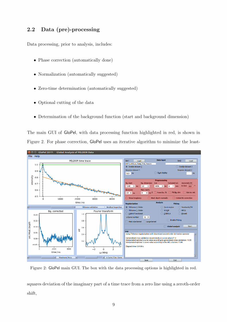
2.2 Data (pre)-processing

Data processing, prior to analysis, includes:

• Phase correction (automatically done)

• Normalization (automatically suggested)

• Zero-time determination (automatically suggested)

• Optional cutting of the data

• Determination of the background function (start and background dimension)

The main GUI of GloPel, with data processing function highlighted in red, is shown in

Figure 2. For phase correction, GloPel uses an iterative algorithm to minimize the least-

Figure 2: GloPel main GUI. The box with the data processing options is highlighted in red.

squares deviation of the imaginary part of a time trace from a zero line using a zeroth-order

shift,

9

2.2.1 Phase correction

Vpc(T ) = exp(i γ0) · Vraw(T ) ., (1)

γ0 is the phase angle in the complex plane. Phase correction is automatically performed

upon loading the raw data and cannot be changed manually.

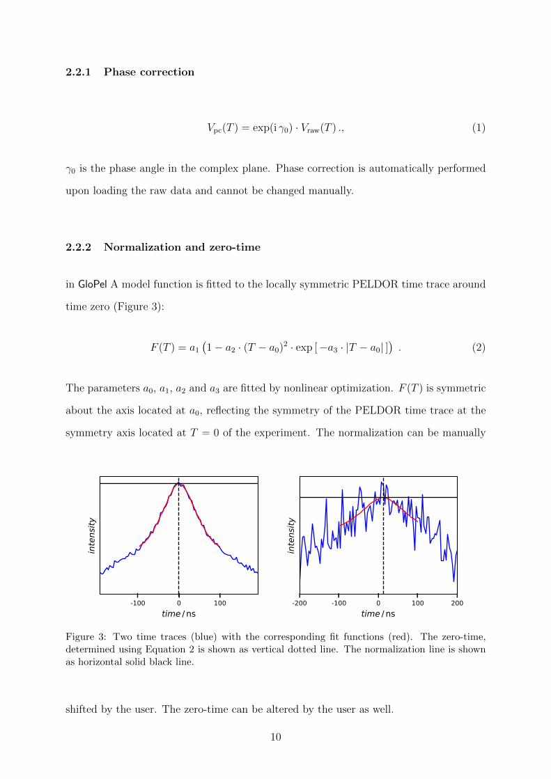
2.2.2 Normalization and zero-time

in GloPel A model function is fitted to the locally symmetric PELDOR time trace around

time zero (Figure 3):

F (T ) = a1

(1− a2 · (T − a0)2 · exp [−a3 · |T − a0| ]

). (2)

The parameters a0, a1, a2 and a3 are fitted by nonlinear optimization. F (T ) is symmetric

about the axis located at a0, reflecting the symmetry of the PELDOR time trace at the

symmetry axis located at T = 0 of the experiment. The normalization can be manually

-100 0 100time / ns

inte

nsity

-200 -100 0 100 200time / ns

inte

nsity

Figure 3: Two time traces (blue) with the corresponding fit functions (red). The zero-time,determined using Equation 2 is shown as vertical dotted line. The normalization line is shownas horizontal solid black line.

shifted by the user. The zero-time can be altered by the user as well.

10

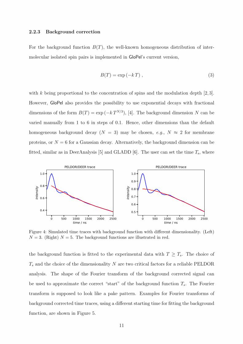
2.2.3 Background correction

For the background function B(T ), the well-known homogeneous distribution of inter-

molecular isolated spin pairs is implemented in GloPel’s current version,

B(T ) = exp (−k T ) , (3)

with k being proportional to the concentration of spins and the modulation depth [2, 3].

However, GloPel also provides the possibility to use exponential decays with fractional

dimensions of the form B(T ) = exp (−k TN/3), [4]. The background dimension N can be

varied manually from 1 to 6 in steps of 0.1. Hence, other dimensions than the default

homogeneous background decay (N = 3) may be chosen, e.g., N ≈ 2 for membrane

proteins, or N = 6 for a Gaussian decay. Alternatively, the background dimension can be

fitted, similar as in DeerAnalysis [5] and GLADD [6]. The user can set the time Ts, where

0 500 1000 1500 2000 2500time / ns

0.4

0.6

0.8

1.0

Inte

nsity

PELDOR/DEER trace

0 500 1000 1500 2000 2500time / ns

0.5

0.6

0.7

0.8

0.9

1.0

Inte

nsity

PELDOR/DEER trace

Figure 4: Simulated time traces with background function with different dimensionality. (Left)N = 3. (Right) N = 5. The background functions are illustrated in red.

the background function is fitted to the experimental data with T ≥ Ts. The choice of

Ts and the choice of the dimensionality N are two critical factors for a reliable PELDOR

analysis. The shape of the Fourier transform of the background corrected signal can

be used to approximate the correct “start” of the background function Ts. The Fourier

transform is supposed to look like a pake pattern. Examples for Fourier transforms of

background corrected time traces, using a different starting time for fitting the background

function, are shown in Figure 5.

11

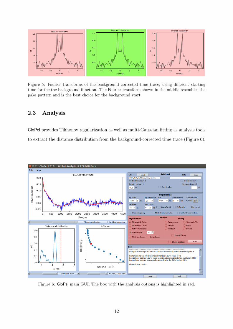
Figure 5: Fourier transforms of the background corrected time trace, using different startingtime for the the background function. The Fourier transform shown in the middle resembles thepake pattern and is the best choice for the background start.

2.3 Analysis

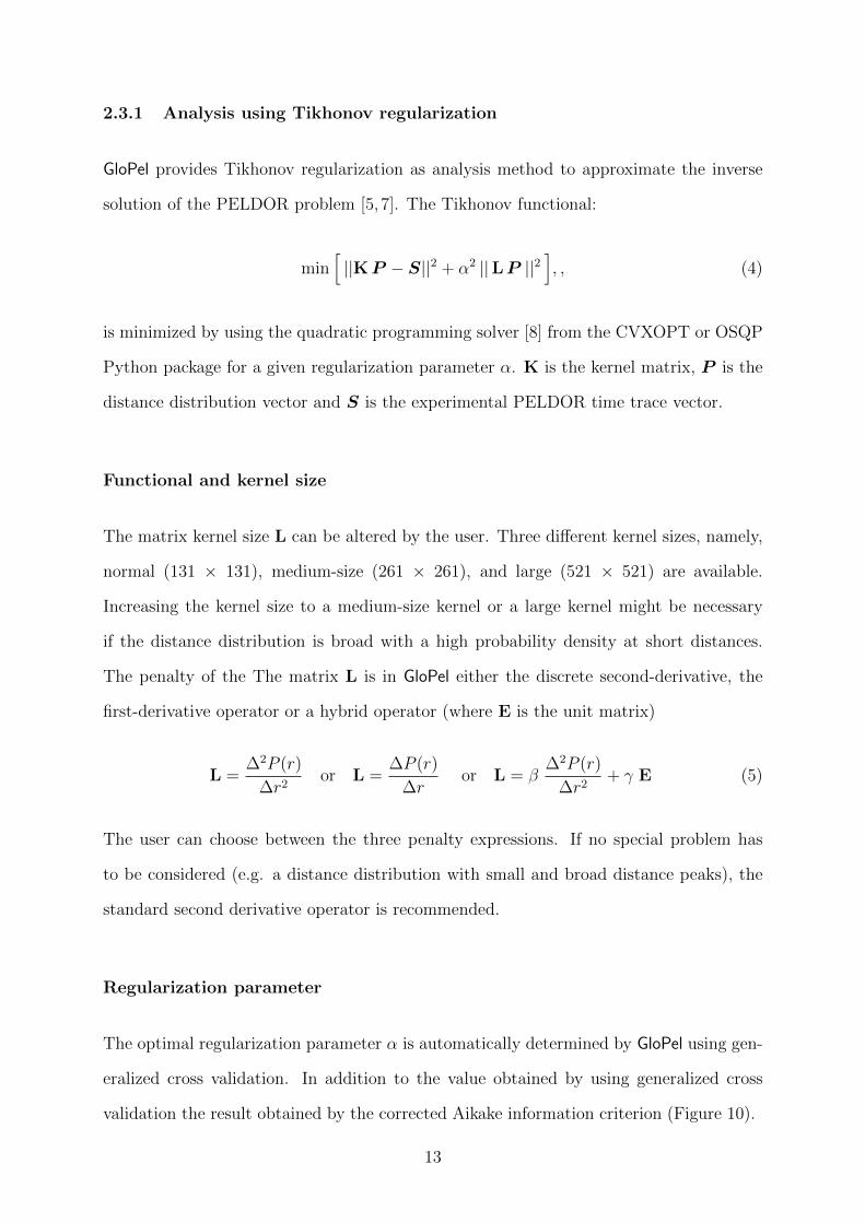
GloPel provides Tikhonov regularization as well as multi-Gaussian fitting as analysis tools

to extract the distance distribution from the background-corrected time trace (Figure 6).

Figure 6: GloPel main GUI. The box with the analysis options is highlighted in red.

12

2.3.1 Analysis using Tikhonov regularization

GloPel provides Tikhonov regularization as analysis method to approximate the inverse

solution of the PELDOR problem [5,7]. The Tikhonov functional:

min[||KP − S||2 + α2 ||LP ||2

], , (4)

is minimized by using the quadratic programming solver [8] from the CVXOPT or OSQP

Python package for a given regularization parameter α. K is the kernel matrix, P is the

distance distribution vector and S is the experimental PELDOR time trace vector.

Functional and kernel size

The matrix kernel size L can be altered by the user. Three different kernel sizes, namely,

normal (131 × 131), medium-size (261 × 261), and large (521 × 521) are available.

Increasing the kernel size to a medium-size kernel or a large kernel might be necessary

if the distance distribution is broad with a high probability density at short distances.

The penalty of the The matrix L is in GloPel either the discrete second-derivative, the

first-derivative operator or a hybrid operator (where E is the unit matrix)

L =∆2P (r)

∆r2or L =

∆P (r)

∆ror L = β

∆2P (r)

∆r2+ γ E (5)

The user can choose between the three penalty expressions. If no special problem has

to be considered (e.g. a distance distribution with small and broad distance peaks), the

standard second derivative operator is recommended.

Regularization parameter

The optimal regularization parameter α is automatically determined by GloPel using gen-

eralized cross validation. In addition to the value obtained by using generalized cross

validation the result obtained by the corrected Aikake information criterion (Figure 10).

13

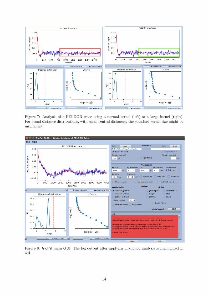
Figure 7: Analysis of a PELDOR trace using a normal kernel (left) or a large kernel (right).For broad distance distributions, with small central distances, the standard kernel size might beinsufficient.

Figure 8: GloPel main GUI. The log output after applying Tikhonov analysis is highlighted inred.

14

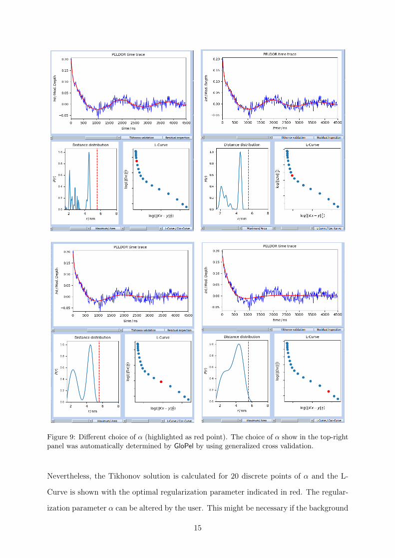
Figure 9: Different choice of α (highlighted as red point). The choice of α show in the top-rightpanel was automatically determined by GloPel by using generalized cross validation.

Nevertheless, the Tikhonov solution is calculated for 20 discrete points of α and the L-

Curve is shown with the optimal regularization parameter indicated in red. The regular-

ization parameter α can be altered by the user. This might be necessary if the background

15

function was not properly determined and the suggested regularization parameter is far

away from the “corner” of the L-Curve. Different values of α for the same PELDOR time

trace are shown in Figure 9.

2.3.2 Model-based fitting

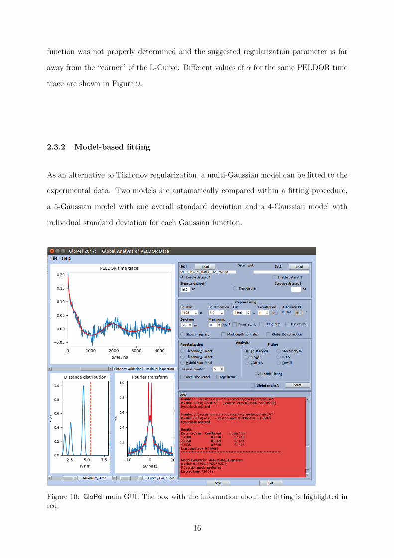
As an alternative to Tikhonov regularization, a multi-Gaussian model can be fitted to the

experimental data. Two models are automatically compared within a fitting procedure,

a 5-Gaussian model with one overall standard deviation and a 4-Gaussian model with

individual standard deviation for each Gaussian function.

Figure 10: GloPel main GUI. The box with the information about the fitting is highlighted inred.

16

The full expression of the fitting function Vfit(T ) used in GloPel is given by

Vfit(T ) =

λ

4(5)∑k=1

fk

j∑i=1

I(rk,i)

π/2∫0

cos(

(1− 3 cos2φ)ωk,i T)

sinφ dφ

with I(rk,i) =1

σk√

2πexp

[−1

2

(rk,0 − rk,i

σk

)2]

and

4(5)∑k=1

fk = 1 with fk ∈ R+0 .

(6)

In a non-linear optimization, using any of the above-mentioned routines, the central po-

sitions of the four (five) Gaussian distributions (rk), the corresponding linear coefficients

(fk), and the single width σ (in case of five Gaussians) or the individual widths σk (in

case of four Gaussians) are fitted. Both models are calculated subsequently, without the

necessity for the user to provide any startup parameters, and the superior model, accord-

ing to the statistical F-test, is taken as fit solution. The full log console output of a fitting

procedure is shown in Script 1.

Script 1: Full output on the log console after applying a multi-Gaussian fit, using the trust-region

algorithm.

∗∗∗∗∗∗∗∗∗∗∗∗∗∗∗∗∗∗∗∗∗∗∗∗∗∗∗∗∗∗∗∗∗∗∗∗∗∗∗∗∗∗∗∗∗∗∗∗∗∗∗∗∗∗∗∗∗∗∗∗∗∗∗∗∗

Algorithm : Trust−reg ion−r e f l e c t i v e

Number o f Gaussians in c u r r e n t l y accepted /new hypothes i s : 4/3

P−value (F−Test ) =0.0 ( Least−squares : 0 .04902 vs . 0 .04903)

Hypothes is accepted






Hypothes is r e j e c t e d

Resu l t s :

Distance / nm C o e f f i c i e n t sigma / nm

17

2 .6635 0 .4576 0 .3210

4 .5099 0 .5424 0 .1139

Least−squares = 0.050109

∗∗∗∗∗∗∗∗∗∗∗∗∗∗∗∗∗∗∗∗∗∗∗∗∗∗∗∗∗∗∗∗∗∗∗∗∗∗∗∗∗∗∗∗∗∗∗∗∗∗∗∗∗∗∗∗∗∗∗∗∗∗∗∗∗

∗∗∗∗∗∗∗∗∗∗∗∗∗∗∗∗∗∗∗∗∗∗∗∗∗∗∗∗∗∗∗∗∗∗∗∗∗∗∗∗∗∗∗∗∗∗∗∗∗∗∗∗∗∗∗∗∗∗∗∗∗∗∗∗∗

Algorithm : Trust−reg ion−r e f l e c t i v e













Resu l t s :

Distance / nm C o e f f i c i e n t sigma / nm

1.7988 0 .1710 0 .1413

2 .6558 0 .2669 0 .1413

4 .5035 0 .5620 0 .1413

Least−squares = 0.049661

∗∗∗∗∗∗∗∗∗∗∗∗∗∗∗∗∗∗∗∗∗∗∗∗∗∗∗∗∗∗∗∗∗∗∗∗∗∗∗∗∗∗∗∗∗∗∗∗∗∗∗∗∗∗∗∗∗∗∗∗∗∗∗∗∗

Model Eva lutat ion . 4 Gaussians /5 Gaussians

p−value : 0.02353122922550579

5 Gaussian model p r e f e r r e d

Elapsed time : 7 .9161 s

In GloPel, six different optimization routines can be used: (1) the trust-region-reflective

algorithm, (2) sequential least-squares programming (SLSQP), (3) Powell’s conjugate di-

rection method, (4) the Broyden-Fletcher–Goldfarb-Shanno (BFGS) algorithm, (5) con-

strained optimization by linear approximation (COBYLA), as implemented in the Python

package Scipy, and (6) a semi-stochastic algorithm.

18

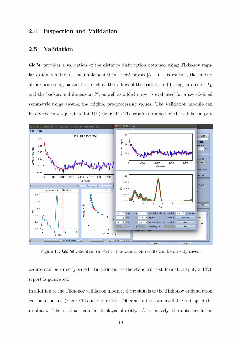
2.4 Inspection and Validation

2.5 Validation

GloPel provides a validation of the distance distribution obtained using Tikhonov regu-

larization, similar to that implemented in DeerAnalysis [5]. In this routine, the impact

of pre-processing parameters, such as the values of the background fitting parameter TD

and the background dimension N , as well as added noise, is evaluated for a user-defined

symmetric range around the original pre-processing values. The Validation module can

be opened in a separate sub-GUI (Figure 11) The results obtained by the validation pro-

Figure 11: GloPel validation sub-GUI. The validation results can be directly saved.

cedure can be directly saved. In addition to the standard text format output, a PDF

report is generated.

In addition to the Tikhonov validation module, the residuals of the Tikhonov or fit solution

can be inspected (Figure 12 and Figure 13). Different options are available to inspect the

residuals. The residuals can be displayed directly. Alternatively, the autocorrelation

19

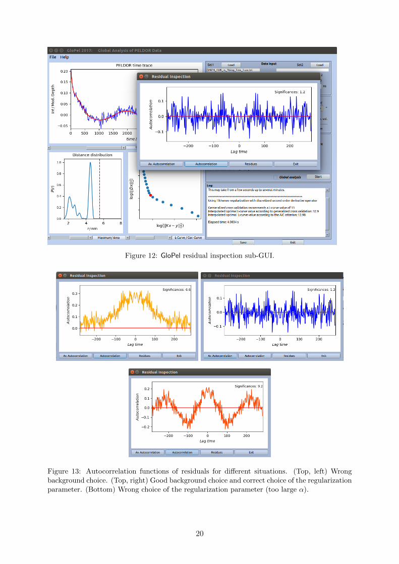
Figure 12: GloPel residual inspection sub-GUI.

Figure 13: Autocorrelation functions of residuals for different situations. (Top, left) Wrongbackground choice. (Top, right) Good background choice and correct choice of the regularizationparameter. (Bottom) Wrong choice of the regularization parameter (too large α).

20

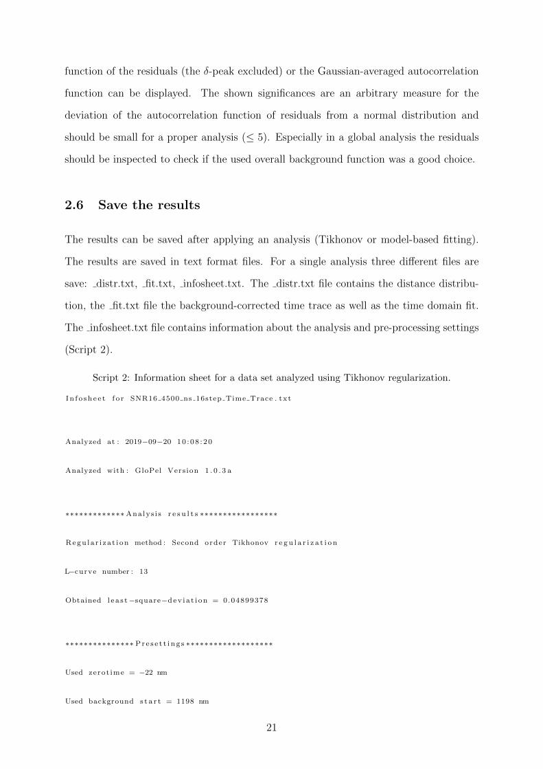
function of the residuals (the δ-peak excluded) or the Gaussian-averaged autocorrelation

function can be displayed. The shown significances are an arbitrary measure for the

deviation of the autocorrelation function of residuals from a normal distribution and

should be small for a proper analysis (≤ 5). Especially in a global analysis the residuals

should be inspected to check if the used overall background function was a good choice.

2.6 Save the results

The results can be saved after applying an analysis (Tikhonov or model-based fitting).

The results are saved in text format files. For a single analysis three different files are

save: distr.txt, fit.txt, infosheet.txt. The distr.txt file contains the distance distribu-

tion, the fit.txt file the background-corrected time trace as well as the time domain fit.

The infosheet.txt file contains information about the analysis and pre-processing settings

(Script 2).

Script 2: Information sheet for a data set analyzed using Tikhonov regularization.

I n f o s h e e t f o r SNR16 4500 ns 16step Time Trace . txt

Analyzed at : 2019−09−20 10 : 08 : 20

Analyzed with : GloPel Vers ion 1 . 0 . 3 a

∗∗∗∗∗∗∗∗∗∗∗∗∗ Analys i s r e s u l t s ∗∗∗∗∗∗∗∗∗∗∗∗∗∗∗∗∗

Regu la r i z a t i on method : Second order Tikhonov r e g u l a r i z a t i o n

L−curve number : 13

Obtained l e a s t −square−dev i a t i on = 0.04899378

∗∗∗∗∗∗∗∗∗∗∗∗∗∗∗ P r e s e t t i n g s ∗∗∗∗∗∗∗∗∗∗∗∗∗∗∗∗∗∗∗

Used zerot ime = −22 nm

Used background s t a r t = 1198 nm

21

Used background dimension = 3

Obtained background decay : k = 0.09982

Obtained modulation depth : lambda = 0.196417

Manual norma l i za t i on = 0E−3

No g l o b a l background func t i on used

No modulation depth norma l i za t i on used

Time t r a c e was cut at : 4496 .0 nm (Raw data maximum time : 4512 .0 nm)

∗∗∗∗∗∗∗∗∗∗∗∗∗∗∗∗∗∗∗∗∗∗∗∗∗∗∗∗∗∗∗∗∗∗∗∗∗∗∗∗∗∗∗∗∗

22

3 Global analysis

GloPel was initially developed for analyzing multiple time traces simultaneously in a global

analysis. However, as for the signal-to-noise problem the analysis of more than two time

traces brought no further improvement, the GloPel GUI is limited to the global analysis of

two time traces. Applications of global analysis are cases, where long and short spin-label

distances simultaneously modulate the primary time-domain curves. In these situations

we recommend to record echo decays that comprise (i) data points with sufficiently narrow

spacing (small step-sizes) within a shorter observation window and good signal-to-noise

ratio, and (ii) data with a wider spacing (larger step-sizes) within a wide observation

window to probe also longer distances and to provide a reliable background curve for

subtraction from both decays.

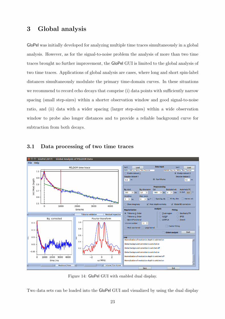
3.1 Data processing of two time traces

Figure 14: GloPel GUI with enabled dual display.

Two data sets can be loaded into the GloPel GUI and visualized by using the dual display

23

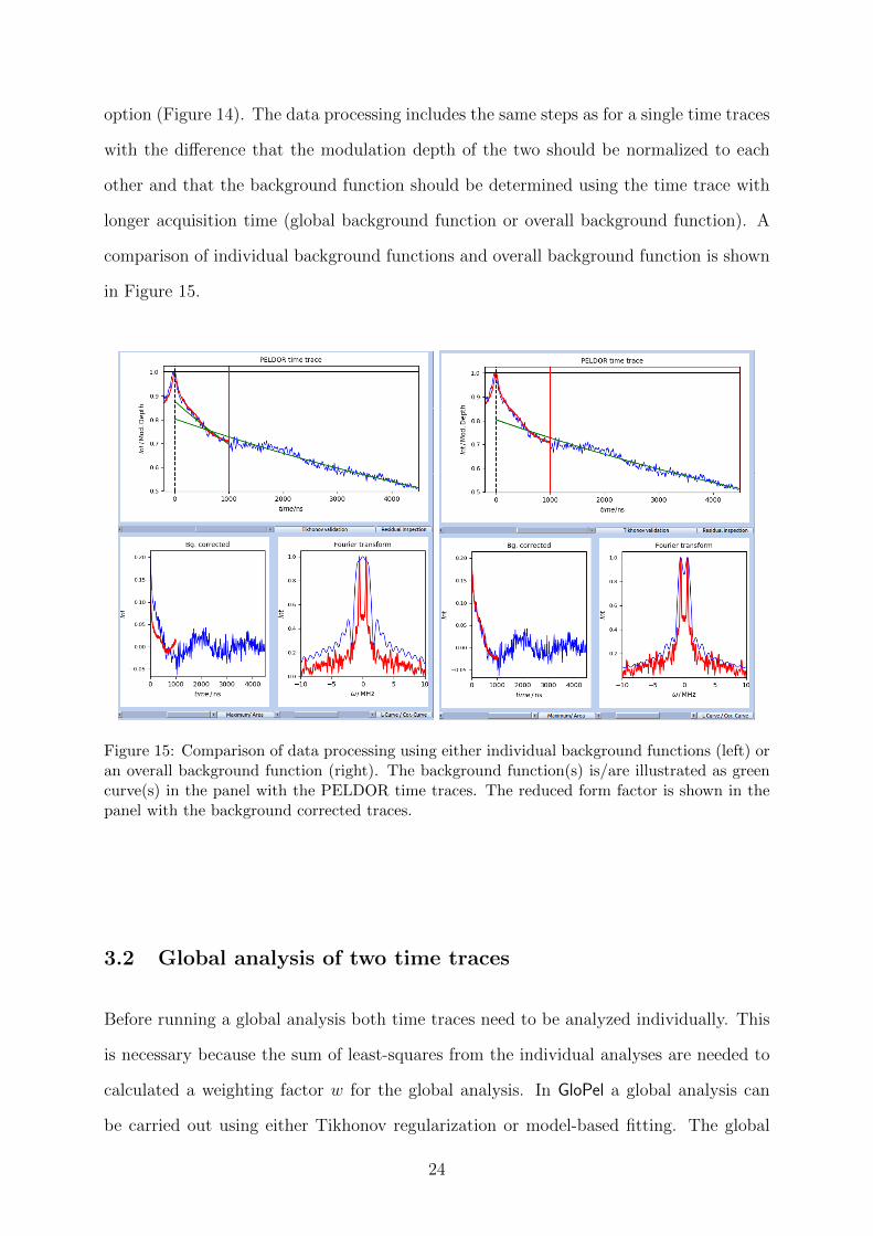
option (Figure 14). The data processing includes the same steps as for a single time traces

with the difference that the modulation depth of the two should be normalized to each

other and that the background function should be determined using the time trace with

longer acquisition time (global background function or overall background function). A

comparison of individual background functions and overall background function is shown

in Figure 15.

Figure 15: Comparison of data processing using either individual background functions (left) oran overall background function (right). The background function(s) is/are illustrated as greencurve(s) in the panel with the PELDOR time traces. The reduced form factor is shown in thepanel with the background corrected traces.

3.2 Global analysis of two time traces

Before running a global analysis both time traces need to be analyzed individually. This

is necessary because the sum of least-squares from the individual analyses are needed to

calculated a weighting factor w for the global analysis. In GloPel a global analysis can

be carried out using either Tikhonov regularization or model-based fitting. The global

24

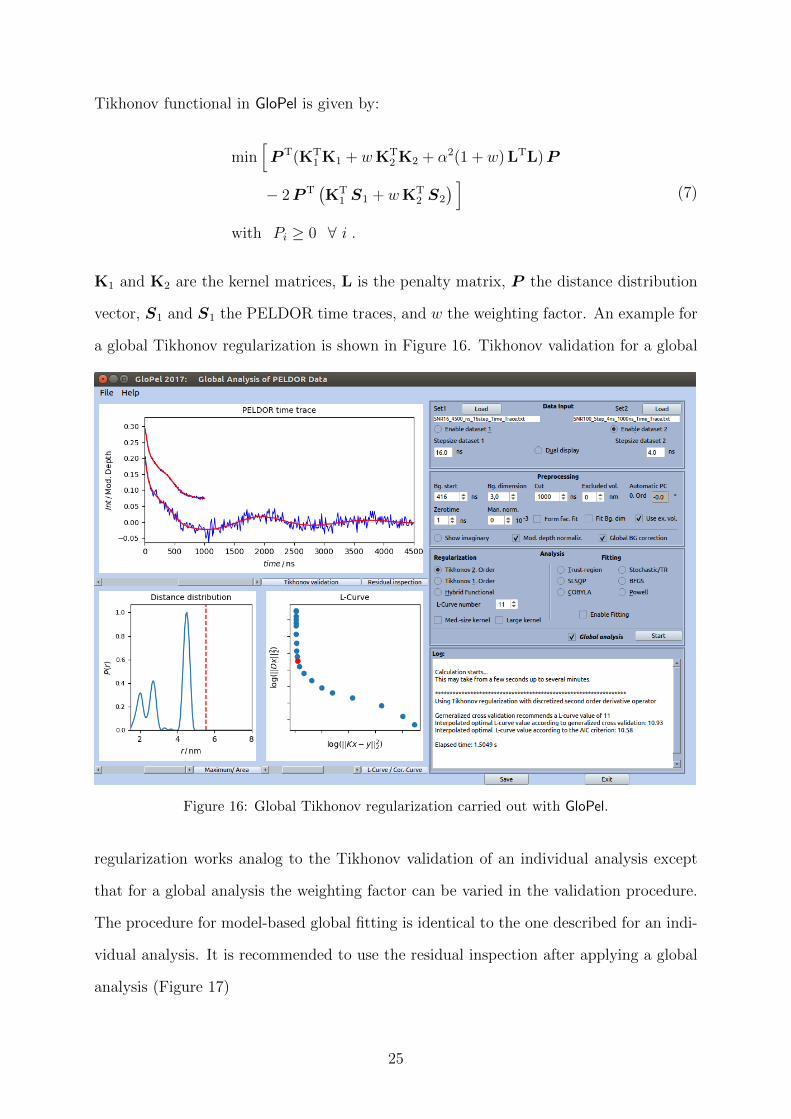
Tikhonov functional in GloPel is given by:

min[P T(KT

1 K1 + wKT2 K2 + α2(1 + w) LTL)P

− 2P T(KT

1 S1 + wKT2 S2

) ]with Pi ≥ 0 ∀ i .

(7)

K1 and K2 are the kernel matrices, L is the penalty matrix, P the distance distribution

vector, S1 and S1 the PELDOR time traces, and w the weighting factor. An example for

a global Tikhonov regularization is shown in Figure 16. Tikhonov validation for a global

Figure 16: Global Tikhonov regularization carried out with GloPel.

regularization works analog to the Tikhonov validation of an individual analysis except

that for a global analysis the weighting factor can be varied in the validation procedure.

The procedure for model-based global fitting is identical to the one described for an indi-

vidual analysis. It is recommended to use the residual inspection after applying a global

analysis (Figure 17)

25

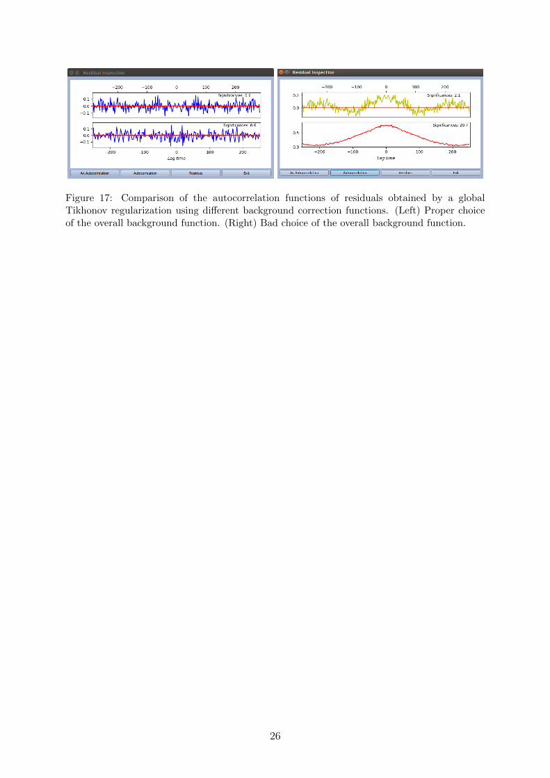
Figure 17: Comparison of the autocorrelation functions of residuals obtained by a globalTikhonov regularization using different background correction functions. (Left) Proper choiceof the overall background function. (Right) Bad choice of the overall background function.

26

References

[1] S. Rein, P. Lewe, S. L. Andrade, S. Kacprzak, and S. Weber. Global analysis of

complex PELDOR time traces. J. Magn. Reson., 295:17–26, 2018.

[2] A.D. Milov, K.M. Salikhov, and M.D. Shirov. Application of ELDOR in electron-spin

echo for paramagnetic center space distribution in solids. Fiz. Tverd. Tela, 23:975–982,

1981.

[3] A.D. Milov, A.B. Ponomarev, and Y.D. Tsvetkov. Electron–electron double resonance

in electron spin echo: model biradical systems and the sensitized photolysis of decalin.

Chem. Phys. Lett., 110:67–72, 1984.

[4] A.D. Milov and Y.D. Tsvetkov. Double electron–electron resonance in electron spin

echo: conformations of spin-labeled poly-4-vinylpyridine in glassy solution. Appl.

Magn. Reson., 12:495–504, 1997.

[5] G. Jeschke, V. Chechik, P. Ionita, A. Godt, H. Zimmermann, J. Banham, C.R. Tim-

mel, D. Hilger, and H. Jung. DeerAnalysis2006 – a comprehensive software package

for analyzing pulsed ELDOR data. Appl. Magn. Reson., 30:473–498, 2006.

[6] S. Brandon, A.H. Beth, and E.J. Hustedt. The global analysis of DEER data. J.

Magn. Reson., 218:93–104, 2012.

[7] Y.-W. Chiang, P. P. Borbat, and J. H. Freed. The determination of pair distance

distributions by pulsed ESR using Tikhonov regularization. J. Magn. Reson., 172:279–

295, 2005.

[8] G. Landi and F. Zama. The active-set method for nonnegative regularization of linear

ill-posed problems. Appl. Math. Comput., 175:715–729, 2006.

27

Documents

GloPel User Manual - radicals.uni-freiburg.de