Globalization and Capital Markets∗

Maurice ObstfeldUniversity of California, Berkeley, CEPR, and NBER†

Alan M. TaylorUniversity of California, Davis, and NBER‡

February 2002

∗This paper was prepared for the NBER conference “Globalization in Historical Perspective”held in Santa Barbara, May 4–5, 2001, and is forthcoming in the NBER conference volume of thesame name edited by Michael D. Bordo, Alan M. Taylor, and Jeffrey G. Williamson. Jay Sham-baugh and Julian di Giovanni provided superb research assistance. For assistance with data wethank Michael Bordo, Gregory Clark, Stephen Haber, Ian McLean, Satyen Mehta, Chris Meissner,and Michael Twomey. For editorial suggestions we thank Michael Bordo. We received helpfulcomments from our discussant Richard Portes; from Marc Flandreau and other conference par-ticipants at Santa Barbara; from Michael Jansson, Lawrence Officer, and Rolf vom Dorp; andfrom participants in seminars at Stanford Graduate School of Business, University of SouthernCalifornia, King’s College, Cambridge, and Universidad Argentina de la Empresa, Buenos Aires.Obstfeld acknowledges the financial support of the National Science Foundation, through a grantadministered by the National Bureau of Economic Research.

†Department of Economics, 549 Evans Hall #3880, University of California, Berkeley, CA94720-3880. Tel: 510-643-9646. Fax: 510-642-6615. Email:<obstfeld@econ.berkeley.edu>.WWW: <http://emlab.berkeley.edu/users/obstfeld/>

‡Address: Department of Economics, University of California, One Shields Avenue, Davis,CA 95616-8578. Tel: 530-752-1572. Fax: 530-752-9382. Email:<amtaylor@ucdavis.edu>.WWW: <http://www.econ.ucdavis.edu/faculty/amtaylor/>.

1 Global Capital Markets: Overview and Origins

At the turn of the twenty-first century, the merits of international financial inte-gration are under more forceful attack than at any time since the 1940s. Evenmainstream academic proponents of free multilateral commodity trade, such asBhagwati, argue that the risks of global financial integration outweigh the benefitsit affords. Critics from the left such as Eatwell, more skeptical even of the casefor free trade on current account, suggest that since the 1960s “free internationalcapital flows” have been “associated with a deterioration in economic efficiency(as measured by growth and unemployment).”1

The resurgence of concerns over international financial integration is under-standable in light of the financial crises in Latin America in 1994-95, East Asiaand Russia in 1997-98, and Argentina in 2001–02. Proponents of free trade intangible goods have long recognized that its net benefits to countries typicallyare distributed unevenly, creating domestic winners and losers. But recent inter-national financial crises have submerged entire economies and threatened theirtrading partners, inflicting losses all around. International financial transactionsrely intrinsically on the expectation that counterparties will fulfill future contractualcommitments; they therefore place confidence and possibly volatile expectationsat center stage.2 These same factors are present in purely domestic financial trades,of course. But oversight, adjudication, and enforcement all are orders of magni-tude more difficult among sovereign nations with distinct national currencies thanwithin a single national jurisdiction. And there is no natural world lender of lastresort, so international crises are intrinsically harder to head off and contain. Fac-tors other than the threat of crises, such as the power of capital markets to constraindomestically-oriented economic policies, also have sparked concerns over greaterfinancial openness.

The ebb and flow of international capital since the nineteenth century illus-trates recurring difficulties, as well as the alternative perspectives from whichpolicymakers have tried to confront them. The subsequent sections are devotedto documenting these vicissitudes quantitatively and explaining them. We believethat economic theory and economic history together can provide useful insightsinto events of the past and deliver relevant lessons for today.

1See Bhagwati (1998); Eatwell (1997, p. 2). For a broad perspective on the future prospects ofeconomic integration in general, see Rodrik (2000).

2The vast majority of commodity trades also involve an element of intertemporal exchange, viadeferred or advance payment for goods, but the unwinding of the resulting cross-border obligationstends to be predictable.

1

1.1 The Emergence of World Capital Markets

Prior to the nineteenth century, the geographical scope for international finance wasrelatively limited compared to what was to come. Italian banks of the Renaissancefinanced trade and government around the Mediterranean, and, as trade expandedwithin Europe, financial innovations spread farther north through the letters ofcredit developed at the Champagne Fairs and the new banks in North Sea portssuch as Bruges and Antwerp. Later, London and Amsterdam became the keycenters, and their currencies and financial instruments were the principal focusof players in the market. As the industrial revolution gathered force and spreadout from Britain, the importance of international financial markets became moreapparent in both the public and private spheres.3

In due course, the scope for such trades extended to other centers that de-veloped the markets and institutions capable of supporting international financialtransactions, and whose governments were not hostile to such developments. Inthe Eastern U.S., a broad range of centers including Boston, Philadelphia, and Bal-timore gave way to what became the dominant center of national and internationalfinance, New York. By the late nineteenth century both France and the Germanyhad developed sophisticated and expanding international markets well-integratedinto the networks of global finance. Elsewhere in Europe and the New Worldsimilar markets began from an embryonic stage, and eventually financial tradingspread to places as far afield as Melbourne and Buenos Aires.4 As we shall dis-cuss later, after 1870 these developments were to progress even further. With theworld starting to converge on the gold standard as a monetary system, and withtechnological developments in shipping (for example, steamships replacing sail,the Panama Canal) and communications (the telegraph, trans-oceanic cables), theconstruction of the first global marketplace in capital, as well as in goods and labor,took hold in an era of undisputed liberalism and virtuallaisser faire.

Within finance, the technological and institutional developments were many:the use of modern communications to transmit prices; the development of a verybroad array of private debt and equity instruments, and the widening scope forinsurance activities; the expanding role of government bond markets internation-

3See Cameron (1993); Neal (1990, 2000); Oppers (1993); Brezis (1995).4On the U.S. see Davis (1965) and Sylla (1975; 1998). On Europe see Kindleberger (1984). For

a comprehensive discussion of the historical and institutional developments in some key countrieswhere international financial markets made an impact at this time—the United Kingdom, theUnited States, Australia, Argentina, and Canada—see Davis and Gallman (2001). On comparativefinancial deepening and sophistication see Goldsmith (1985).

2

ally; and the more widespread use of forward and futures contracts, and derivativesecurities. By 1900, the use of such instruments permeated the major economiccenters of dozens of countries around the world, stretching from Europe, east andwest, north to south, to the Americas, Asia, and Africa. The key currencies andinstruments were known everywhere, and formed the basis for an expanding worldcommercial network, whose rise was equally meteoric. Bills of exchange, bondfinance, equity issues, foreign direct investments, and many other types of transac-tions were by then quite common among the core countries, and among a growingnumber of nations at the periphery.

Aside fromhaute finance, more and more day-to-day activities came into theorbit of finance via the growth and development of banking systems in manycountries, offering checking and saving accounts as time passed. This in turnraised the question of whether banking supervision would be done by the banksthemselves or the government authorities, with solutions including free bankingand “wildcat” banks (as in the United States), and changing over time to includesupervisory functions as part of a broader central monetary authority, the centralbank. From what was once an esoteric sector of the economy, the financial sectorgrew locally and globally to touch an ever-expanding range of activity.5

Thus, the scope for capital markets to do good—or do harm—loomed largeras time went by. As an ever-greater part of national and international economiesbecame monetized and sensitive to financial markets, agents in all spheres—publicand private, labor and capital, domestic and foreign—were affected. Who stoodto gain or lose? What policies would emerge as government objectives evolved?Would global capital markets proceed unfettered or not? From the turn of thetwentieth century, the unfolding history of the international capital market hasbeen of enormous import. The market has undoubtedly shaped the course ofnational and international economic development and swayed political interests inall manner of directions at various times. In terms of distribution and equality, ithas made winners and losers, though so often is the process misunderstood thatthe winners and losers are often unclear, at the national and the global level. Anaim of this paper is to tell the history of what became a trulyglobal capital marketon the eve of the twentieth century, and explore how it has influenced the courseof events ever since.

5On financial development see the chapter by Rousseau and Sylla in this volume.

3

1.2 Stylized Facts for the Nineteenth and Twentieth Century

Notwithstanding the undisputed record of technological advancement and eco-nomic growth over the long run, we must reject the temptations of a simple linearhistory as we examine international capital markets and their evolution. It has notbeen a record of ever-more-perfectly-functioning markets with ever-lower transac-tion costs and ever-expanding scope. The mid-twentieth century, on the contrary,was marked by an enormous reaction against markets, international as well as do-mestic, and against financial markets in particular.6 Muted echoes of these samethemes could be heard once again at the end of the twentieth century.

What do we already know about the evolution of global capital mobility inthe last century or more? Very few previous studies exist for the entire period andcovering a sufficiently comprehensive cross-section of countries; but many authorshave focused on individual countries and particular epochs, and from their workwe can piece together a working set of hypotheses which might be termed theconventional wisdom concerning the evolution of international capital mobility inthe post-1870 era. The story comes in four parts, and not coincidentally these echothe division of the twentieth century into distinct international monetary regimes.7

The first period runs up to 1914. After 1870 an increasing share of the worldeconomy came into the orbit of the classical gold standard, and a global capitalmarket centered on London. By 1880, quite a few countries were on gold, and by1900 a large number. This fixed exchange-rate system was for most countries astable and credible regime, and functioned as a disciplining or commitment device.Accordingly, interest rates across countries tended to converge, and capital flowssurged. Many peripheral countries, not to mention the New World offshoots ofWestern Europe, took part in an increasingly globalized economy in not only thecapital market, but also goods and labor markets.8

In the second period, from 1914 to 1945, this global economy was destroyed.Two world wars and a Great Depression accompanied a rise in nationalism andincreasingly noncooperative economic policymaking. With gold-standard cred-

6See Polanyi (1944).7On this division of history see, in particular, Eichengreen (1996). Earlier surveys of the

progress of financial-market globalization since the nineteenth century include Obstfeld and Taylor(1998), Bordo, Eichengreen, and Kim (1999), and Flandreau and Rivière (1999).

8On the gold-standard regime and late-nineteenth-centurycapital markets see,inter alia, Eichen-green (1996); Eichengreen and Flandreau (1996); Bordo and Kydland (1995); Bordo and Rockoff(1996); Edelstein (1982). On this first era of globalization in goods and factor markets see Sachsand Warner (1993); Williamson (1996); O’Rourke and Williamson (1999); and chapters by Findlayand O’Rourke, and Chiswick and Hatton, in this volume.

4

ibility broken by World War One, monetary policy became subject to domesticpolitical goals, first as a way to help finance wartime deficits. Later, monetary pol-icy was a tool to engineer beggar-thy-neighbor devaluations under floating rates.As a guard against currency crises and to protect gold, capital controls becamewidespread. The world economy went from globalized to almost autarkic in thespace of a few decades. Capital flows were minimal, international investment wasregarded with suspicion, and international prices and interest rates fell completelyout of synchronization. Global capital was demonized, and seen as one of theprincipal causes of the international depression of the 1930s.9

In the third period, the Bretton Woods era (1945–71), an attempt to rebuildthe global economy took shape. Trade flows began a remarkable expansion, andeconomic growth began its most rapid spurt in history worldwide. Yet fears formedin the interwar period concerning global capital were not easily dispelled. TheIMF initially sanctioned capital controls as a means to prevent currency crises andruns, and this lent some autonomy to governments by providing more power toactivist monetary policy. For twenty years, this prevailing philosophy held firm;and although capital markets recovered, they did so slowly. But by the late 1960sglobal capital could not be held back so easily, and its workings eventually brokethe compromise that had sustained the fixed exchange-rate system.10

In the fourth and final period, the post-Bretton Woods floating-rate era, a dif-ferent trend has been evident. Although fixed-rate regimes were reluctantly givenup, and though some countries still attempt to maintain or create such regimesanew, the years from the 1970s to the 1990s have been characterized by a seemingincrease in capital mobility. Generally speaking, industrial-country governmentsno longer needed capital controls as a tool to help preserve a fixed exchange-ratepeg, since the peg was gone. As a floating rate could accommodate market sen-timent, controls could be lifted. This was encouraging to the flow of capital inall countries. In peripheral countries, economic reforms reduced the transactionscosts and risks of foreign investment, and capital flows grew there too—at least un-til the crises of the latter 1990s reminded investors of the fragility of the fixed-rateregimes that tended to persist in the developing world. Increasingly the smallerperipheral countries that desire fixed exchange rates seek credibly to give up do-mestic monetary policy autonomy through currency boards or even dollarization,whereas larger developing countries such as Mexico, Chile, and Brazil have opted

9See Eichengreen (1992; 1996) and Temin (1989). In labor markets migrations collapsed and ingoods markets trade barriers multiplied (Kindleberger 1986, 1989; Williamson 1995; James 2001).

10On Bretton Woods see, for example, Bordo and Eichengreen eds. (1993); Eichengreen (1996).

5

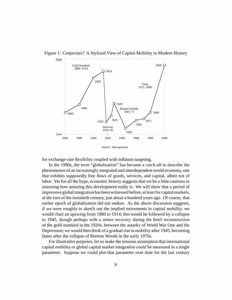
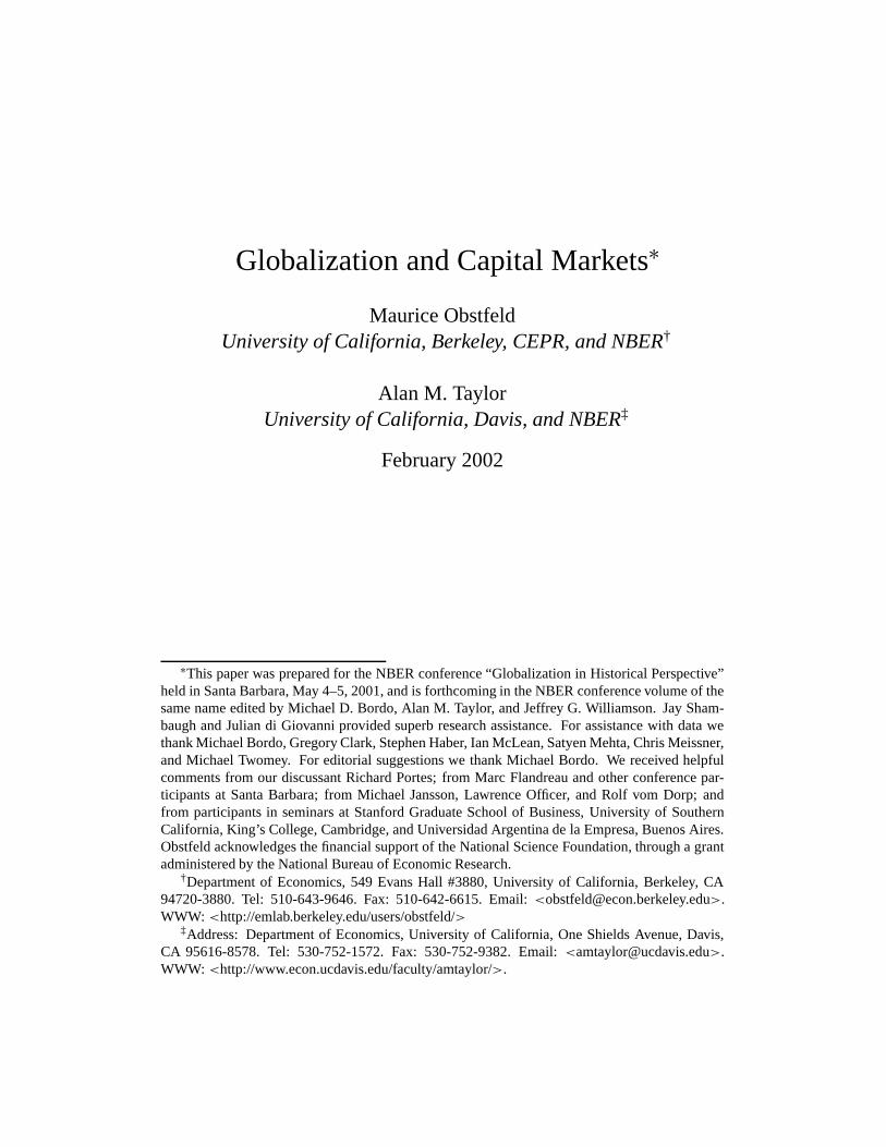
Figure 1: Conjecture? A Stylized View of Capital Mobility in Modern History

1914

2000

1880

19711918 1925

1929

1945

1960

19801860

1900

1860 1880 1900 1920 1940 1960 1980 2000

Gold Standard1880–1914

Bretton Woods1945–71

Float1971–2000

Interwar1914–45

High

Low

Source: Introspection.

for exchange-rate flexibility coupled with inflation targeting.In the 1990s, the term “globalization” has became a catch-all to describe the

phenomenon of an increasingly integrated and interdependent world economy, onethat exhibits supposedly free flows of goods, services, and capital, albeit not oflabor. Yet for all the hype, economic history suggests that we be a little cautious inassessing how amazing this development really is. We will show that a period ofimpressive global integration has been witnessed before,at least for capital markets,at the turn of the twentieth century, just about a hundred years ago. Of course, thatearlier epoch of globalization did not endure. As the above discussion suggests,if we were roughly to sketch out the implied movements in capital mobility, wewould chart an upswing from 1880 to 1914; this would be followed by a collapseto 1945, though perhaps with a minor recovery during the brief reconstructionof the gold standard in the 1920s, between the autarky of World War One and theDepression; we would then think of a gradual rise in mobility after 1945, becomingfaster after the collapse of Bretton Woods in the early 1970s.

For illustrative purposes, let us make the tenuous assumption that internationalcapital mobility or global capital market integration could be measured in a singleparameter. Suppose we could plot that parameter over time for the last century

6

or so. We would then expect to see a time path something like Figure 1, wherethe vertical axis carries the mobility or integration measure. It is reasonable,given the specific histories of various subperiods or certain countries, as containedin numerous fragments of the historical literature, to speak of capital mobilityincreasing or decreasing at the times we have noted. Thus, the overall ∪-shape ofthis figure is probably correct.

However, without further quantification the usefulness of the stylized viewremains unclear. For one thing, we do not know if it accords with empiricalmeasures of capital mobility. Moreover, even if we know the direction of changesin the mobility of capital at various times, we cannot measure the extent of thosechanges. Without such evidence, we cannot assess whether the ∪-shaped path iscomplete: that is, have we now reached a degree of capital mobility that is above,or still below, that seen in the years before 1914? To address these questionsrequires more formal empirical testing, and that is one of the motivations for thequantitative analysis which follows.

1.3 The Trilemma: Capital Mobility, the Exchange Rate, andMonetary Policy

We seek in this paper not only to offer evidence in support of the stylized view ofglobal capital market evolution, but also to provide an organizing framework forunderstanding that evolution and the forces that shaped the international economyof the late-nineteenth and twentieth centuries. Given the stylized description, wemust address the question: what explains the long stretch of high capital mobilitythat prevailed before 1914, the subsequent breakdown in the interwar period, andthe very slow postwar reconstruction of the world financial system? The answeris tied up with one of the central and most visible areas in which openness to theworld capital market constrains government power: the choice of an exchange rateregime.11

The macroeconomic policy trilemma for open economies (also known as the“ inconsistent trinity” proposition) follows from a basic fact: An open capital marketdeprives a country’s government of the ability simultaneously to target its exchangerate and to use monetary policy in pursuit of other economic objectives. Thetrilemma arises because a macroeconomic policy regime can include at most twoelements of the “ inconsistent trinity” of three policy goals:

11This section draws on Obstfeld and Taylor (1998), who invoked the term “ trilemma,” andObstfeld (1998).

7

(i) full freedom of cross-border capital movements;(ii) a fixed exchange rate; and(iii) an independent monetary policy oriented toward domestic objectives.If capital movements are prohibited, in the case where element (i) is ruled

out, a country on a fixed exchange rate can break ranks with foreign interest ratesand thereby run an independent monetary policy. Similarly a floating exchangerate, in the case where element (ii) is ruled out, reconciles freedom of internationalcapital movements with monetary-policy effectiveness (at least when some nominaldomestic prices are sticky). But monetary policy is powerless to achieve domesticgoals when the exchange rate is fixed and capital movements free, the case whereelement (iii) is ruled out, since intervention in support of the exchange parity thenentails capital flows that exactly offset any monetary-policy action threatening toalter domestic interest rates.12

Our central proposition is that secular movements in the scope of internationallending and borrowing may be understood in terms of this trilemma. Capitalmobility has prevailed and expanded under circumstances of widespread politicalsupport either for an exchange-rate-subordinated monetary regime (for example,the gold standard), or for a monetary regime geared mainly toward domestic ob-jectives at the expense of exchange-rate stability (for example, the recent float).The middle ground in which countries attempt simultaneously to hit exchange-ratetargets and domestic policy goals has, almost as a logical consequence, entailedexchange controls or other harsh constraints on international transactions.

It is this conflict among rival policy choices, the trilemma, that informs ourdiscussion of the historical evolution of world capital markets in the pages thatfollow, and helps make sense of the ebb and flow of capital mobility in the longrun and in the broader political-economy context. Of course, the trilemma is onlya proximate explanation, in the sense that deeper socio-political forces explain therelative dominance of some policy targets over others.

12The choice between fixed and floating exchange rates should not be viewed as dichotomous;nor should it be assumed that the choice of a floating-rate regime necessarily leads to a usefuldegree of monetary-policy flexibility. In reality, the degree of exchange-rate flexibility lies on acontinuum, with exchange-rate target zones, crawling pegs, crawling zones, and managed floatsof various other kinds residing between the extremes of irrevocably fixed and freely floating.The greater the attention given to the exchange rate, the more constrained monetary policy is inpursuing other objectives. Indeed, the notion of a “ free” fl oat is an abstraction with little empiricalcontent, as few governments are willing to set monetary policy without some consideration ofits exchange-rate effects. If exchange rates are subject to pure speculative shocks unrelated toeconomic fundamentals, and if policy makers are concerned to counter these movements, thenmonetary control will be compromised.

8

1.4 A Brief Narrative

The broad trends and cycles in the world capital market that we will documentreflect changing responses to the fundamental trilemma. Before 1914, each of theworld’s major economies pegged its currency’s price in terms of gold, and thus,implicitly, maintained a fixed rate of exchange against every other major country’scurrency. Financial interests ruled the world of the classical gold standard andfinancial orthodoxy saw no alternative mode of sound finance.13 Thus, the goldstandard system met the trilemma by opting for fixed exchange rates and capitalmobility, sometimes at the expense of domestic macroeconomic health. Between1891 and 1897, for example, the United States Treasury put the country througha harsh deflation in the face of persistent speculation on the dollar’s departurefrom gold. These policies were hotly debated; the Populist movement agitatedforcefully against gold, but lost.14

The balance of political power began to change only with the First WorldWar, which brought a sea-change in the social contract underlying the industrialdemocracies. Organized labor emerged as a political power, a counterweight to theinterests of capital, as seen in the British labor unrest of the 1920s, which culmi-nated in a General Strike. Britain’s return to gold in 1925 led the way to a restoredinternational gold standard and a limited resurgence of international finance, butweaknesses in the rebuilt system helped propagate a worldwide depression afterthe 1929 New York stock market crash. Following (and in some cases anticipating)Britain’s example, many countries abandoned the gold standard in the early 1930sand depreciated their currencies; many also resorted to trade and capital controls inorder to manage independently their exchange rates and domestic policies. Thosecountries in the “gold bloc,” which stubbornly clung to gold through the mid-1930s,showed the steepest output and price-level declines. But eventually, in the 1930s,all countries jettisoned rigid exchange-rate targets and/or open capital markets infavor of domestic macroeconomic goals.15

These decisions reflected the shift in political power solidified by the FirstWorld War. They also signaled the beginnings of a new consensus on the roleof economic policy that would endure through the inflationary 1970s. As animmediate consequence, however, the Great Depression discredited gold-standardorthodoxy and brought Keynesian ideas about macroeconomic management to

13See Bordo and Schwartz (1984); Eichengreen (1996).14See Frieden (1997).15See Eichengreen and Sachs (1985); Temin (1989); Eichengreen (1992); Bernanke and Carey

(1996); Obstfeld and Taylor (1998).

9

the fore. It also made financial markets and financial practitioners unpopular.Their supposed excesses and attachment to gold became identified in the publicmind as causes of the economic calamity. In the United States, the New Dealbrought a Jacksonian hostility toward eastern (read: New York) high finance backto Washington. Financial products and markets were banned or more closelyregulated, and the Federal Reserve was brought under heavier Treasury influence.Similar reactions occurred in other countries.

Changed attitudes toward financial activities and economic management under-lay the new postwar economic order negotiated at Bretton Woods, New Hampshire,in July 1944. Forty-four allied countries set up a system based on fixed, but ad-justable, exchange parities, in the belief that floating exchange rates would exhibitinstability and damage international trade. At the center of the system was theInternational Monetary Fund (IMF). The IMF’s prime function was as a source ofhard-currency loans to governments that might otherwise have to temporarily puttheir economies into recession to maintain a fixed exchange rate. Countries ex-periencing permanent balance-of-payments problems had the option of realigningtheir currencies, subject to IMF approval.16

Importantly, the IMF’s founders viewed its lending capability as primarily asubstitute for, not a complement to, private capital inflows. Interwar experience hadgiven the latter a reputation as unreliable at best and, at worst, a dangerous sourceof disturbances. Broad, encompassing controls over private capital movement,perfected in wartime, were expected to continue. The IMF’s Articles of Agreementexplicitly empowered countries to impose new capital controls. Articles VIII andXIV of the IMF agreement did demand that countries’ currencies eventually bemade convertible—in effect, freely saleable to the issuing central bank, at theofficial exchange parity, for dollars or gold. But this privilege was to be extendedonly if the country’s currency had been earned through current account transactions.Convertibility on capital account, as opposed to current-account convertibility, wasnot viewed as mandatory or desirable.

Unfortunately, a wide extent even of current-account convertibility took manyyears to achieve, and even then it was often restricted to nonresidents. In theinterim, countries resorted to bilateral trade deals that required balanced or nearlybalanced trade between every pair of trading partners. If France had an exportsurplus with Britain, and Britain a surplus with Germany, Britain could not useits excess marks to obtain dollars with which to pay France. Germany had veryfew dollars and guarded them jealously for critical imports from the Americas.

16On the Bretton Woods system, see Bordo and Eichengreen (1993).

10

Instead, each country would try to divert import demand toward countries withhigh demand for its goods, and to direct its exports toward countries whose goodswere favored domestically.

Convertibility gridlock in Europe and its dependencies was ended througha regional multilateral clearing scheme, the European Payments Union (EPU).The clearing scheme was set up in 1950 and some countries reached de factoconvertibility by mid-decade. But it was not until December 27, 1958 that Europeofficially embraced convertibility and ended the EPU. Although most Europeancountries still chose to retain extensive capital controls (Germany being the mainexception), the return to convertibility, important as it was in promoting multilateraltrade growth, also increased the opportunities for disguised capital movements.These might take the form, for example, of misinvoicing, or of accelerated ordelayed merchandise payments. Buoyant growth encouraged some countries infurther financial liberalization, although the U.S., worried about its gold losses,raised progressively higher barriers to capital outflow over the 1960s. Eventually,the Bretton Woods system’s very successes hastened its collapse by resurrectingthe trilemma.17

Key countries in the system, notably the U.S. (fearful of slower growth) andGermany (fearful of higher inflation), proved unwilling to accept the domesticpolicy implications of maintaining fixed rates. Even the limited capital mobilityof the early 1970s proved sufficient to allow furious speculative attacks on themajor currencies, and after vain attempts to restore fixed dollar exchange rates, theindustrial countries retreated to floating rates early in 1973. Although viewed atthe time as a temporary emergency measure, the floating-dollar-rate regime is stillwith us a thirty years later.

Floating exchange rates have allowed the explosion in international financialmarkets experienced over the same three decades. Freed from one element of thetrilemma—fixed exchange rates—countries have been able to open their capitalmarkets while still retaining the flexibility to deploy monetary policy in pursuit ofnational objectives. No doubt the experience gained after the inflationary 1970s inanchoring monetary policy to avoid price instability has helped to promote ongoingfinancial integration. Perhaps for the first time in history, countries have learnedhow to keep inflation in check under fiat monies and floating exchange rates.

There are several potentially valid reasons, however, for countries to still fixtheir exchange rates—for example, to keep a better lid on inflation or to counterexchange-rate instability due to financial-market shocks. Such arguments may find

17See Triffin (1957), Einzig (1968), and Eichengreen and Bordo (2001).

11

particular resonance, of course, in developing countries. However, few countriesthat have tried to fix have succeeded for long; eventually, exchange-rate stabilitytends to come into conflict with other policy objectives, the capital markets catchon to the government’s predicament, and a crisis adds enough economic pain tomake the authorities give in. In recent years only a very few major countries haveobserved the discipline of fixed exchange rates for at least five years, and most ofthose were rather special cases.18

One puzzling case, Thailand, dropped off the list in 1997—with a resoundingcrash. Even Hong Kong, which operates a currency board supposedly subordinatedto maintaining the Hong Kong-U.S. dollar peg, suffered repeated speculative at-tacks in the Asian crisis period. Another currency-board experiment, Argentina,held to its 1:1 dollar exchange rate from April 1991 for a remarkable stint of morethan ten years. To accomplish that feat, the country relied on IMF and privatecredit and, despite episodes of growth, endured levels of unemployment higherthan many countries could tolerate. It suffered especially acutely after Brazilmoved to a float in January 1999. Three years later Argentina’s political and eco-nomic arrangements collapsed in external default (December 2001) and currencycollapse (January-February 2002). The European Union members that maintainedmutually fixed rates prior to January 1999 were aided by market confidence in theirown planned solution to the trilemma, a near-term currency merger.

For most larger countries, the trend toward greater financial openness has beenaccompanied—inevitably, we would argue—by a declining reliance on peggedexchange rates in favor of greater exchange-rate flexibility. Some countries haveopted for a different solution, however, adopting extreme straitjackets for monetarypolicy in order to peg an exchange rate. If monetary policy is geared towarddomestic considerations, capital mobility or the exchange-rate target must go. If,instead, fixed exchange rates and integration into the global capital market are theprimary desiderata, monetary policy must be subjugated to those ends.

The details of this argument require a book-length discourse (Obstfeld andTaylor 2002), which allows a full survey of the empirical evidence and the historicalrecord, but we can already pinpoint the key turning points (see Table 1). TheGreat Depression stands as the watershed here, in that it was caused by an ill-advised subordination of monetary policy to an exchange-rate constraint (the goldstandard), which led to a chaotic time of troubles in which countries experimented,typically noncooperatively, with alternative modes of addressing the fundamentaltrilemma. Interwar experience, in turn, discredited the gold standard and led to a

18See Obstfeld and Rogoff (1995).

12

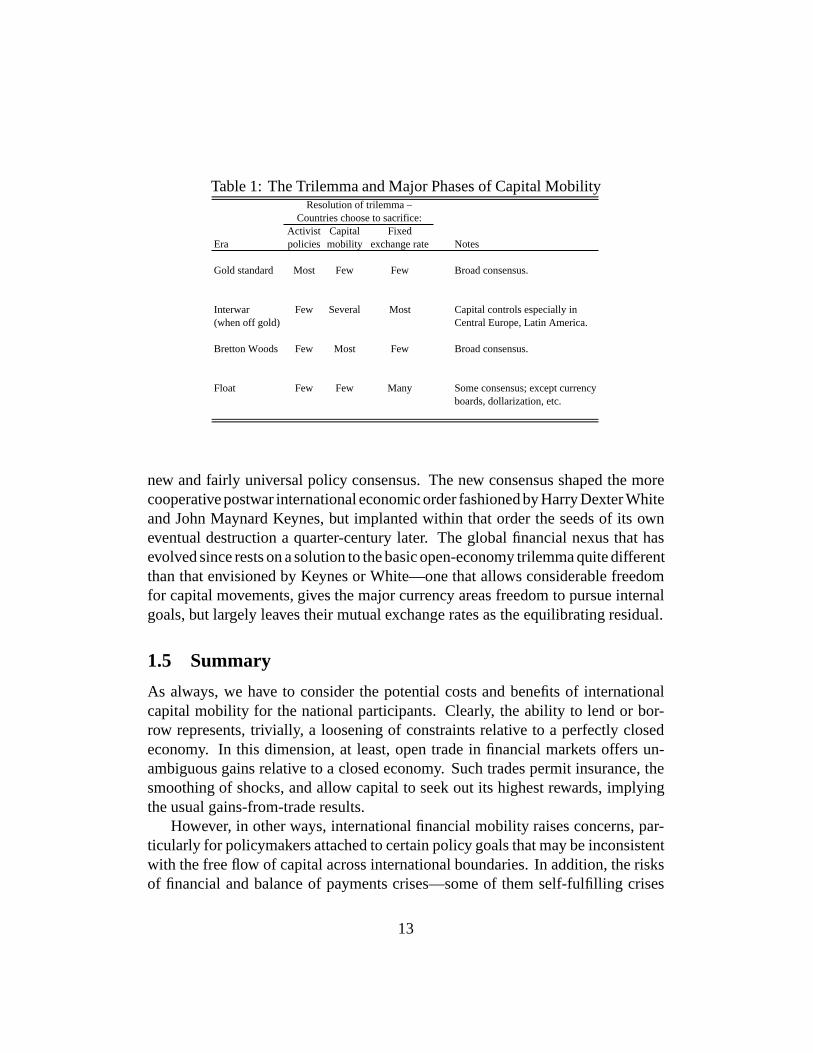
Table 1: The Trilemma and Major Phases of Capital MobilityResolution of trilemma –

Countries choose to sacrifice:Activist Capital Fixed

Era policies mobility exchange rate Notes

Gold standard Most Few Few Broad consensus.

Interwar Few Several Most Capital controls especially in(when off gold) Central Europe, Latin America.

Bretton Woods Few Most Few Broad consensus.

Float Few Few Many Some consensus; except currencyboards, dollarization, etc.

new and fairly universal policy consensus. The new consensus shaped the morecooperative postwar international economic order fashioned by Harry Dexter Whiteand John Maynard Keynes, but implanted within that order the seeds of its owneventual destruction a quarter-century later. The global financial nexus that hasevolved since rests on a solution to the basic open-economy trilemma quite differentthan that envisioned by Keynes or White—one that allows considerable freedomfor capital movements, gives the major currency areas freedom to pursue internalgoals, but largely leaves their mutual exchange rates as the equilibrating residual.

1.5 Summary

As always, we have to consider the potential costs and benefits of internationalcapital mobility for the national participants. Clearly, the ability to lend or bor-row represents, trivially, a loosening of constraints relative to a perfectly closedeconomy. In this dimension, at least, open trade in financial markets offers un-ambiguous gains relative to a closed economy. Such trades permit insurance, thesmoothing of shocks, and allow capital to seek out its highest rewards, implyingthe usual gains-from-trade results.

However, in other ways, international financial mobility raises concerns, par-ticularly for policymakers attached to certain policy goals that may be inconsistentwith the free flow of capital across international boundaries. In addition, the risksof financial and balance of payments crises—some of them self-fulfilling crises

13

unrelated to “ fundamentals”—may represent further obstacles to the adoption offree capital markets.

Although these are very much contemporary issues in world capital markets,the questions they raise can be traced back to the very founding of internationalfinancial markets centuries ago during the Renaissance. Then too, advanced formsof financial asset trades developed very quickly, sometimes as a response to Church-imposed constraints such as usury proscriptions. Financial innovation was subjectto suspicion from various quarters, both public and private. Thus, calls for theregulation and restriction of financial market activity have been with us since theearliest days.

Despite these fears, by the late nineteenth century a succession of technologicalbreakthroughs, and a gradual institutional evolution, had positioned many nationsin a newly forming international capital market. This network of nations embracedmodern financial instruments and operated virtually free of controls on the part ofgovernments. Under the gold standard monetary regime, this flourishing globalmarket for capital reached at least a local peak in the decades just prior to WorldWar One.

Subsequent history showed that this seemingly-linear path toward ever moretechnological progress and institutional sophistication in a liberal world order couldindeed be upset. Two global wars and a depression led the world down an autarkicpath. Conflicting policy goals and democratic tensions often put the interests ofglobal capital at a low premium relative to other objectives. Activist governmentsappealed to capital controls to sidestep the discipline of external markets, and sofree monetary policy for use as a tool of macroeconomic control.

These events demonstrate the power of the macroeconomic policy trilemma toaccount for many of the ups and downs in global capital market evolution in thetwentieth century. In the next section, we match up these stylized facts with someof the quantitative and institutional record, so as to better document the courseof events. It is a remarkable history without which today’s economic, financial,political, and institutional landscape cannot be fully understood.

2 Evidence

In theory and practice, the extent of international capital mobility can have profoundimplications for the operation of individual and global economies. With respectto theory, the applicability of various classes of macroeconomic models rests onmany assumptions, and not the least important of these are axioms linked to the

14

closure of the model in the capital market. The predictions of a theory and itsusefulness for policy debates can revolve critically on this part of the structure.

The importance of these issues for policy is not surprising at all: a moment’sreflection on practical aspects of macroeconomic policy choice underscores the im-pact that capital mobility can have on the efficacy of various interventions: trivially,if capital is perfectly mobile, this dooms to failure any attempts to manipulate localasset prices to make them deviate from global prices, including the most criticalmacroeconomic asset price, the interest rate. Thus, the feasibility and relevance ofkey policy actions cannot be judged absent some informed position on the extentto which local economic conditions are in any way separable from global condi-tions. This means an empirical measure of market integration is implicitly, thoughrarely explicitly, a necessary adjunct to any policy discussion. Although recentglobalization trends have brought this issue to the fore, we show in this paper howthe experience of longer-run macroeconomic history can clarify and inform thesedebates.

In attacking the problem of measuring market integration, economists have nouniversally recognized criterion to turn to. For example, imagine the simple expe-dient of examining price differentials: prices would be identical in two identicalneighboring economies, being determined in each by the identical structures oftastes, technologies, and endowments; but if the two markets were physically sep-arated by an infinitely high transaction-cost barrier one could hardly describe themas being integrated in a single market, as the equality of prices was merely a chanceevent. Or consider looking at the size of flows between two markets as a gaugeof mobility; this is an equally flawed criterion, for suppose we now destroyed thebarrier between the two economies just mentioned, and reduced transaction coststo zero; we would then truly have a single integrated market, but, since on eitherside of the barrier prices were identical in autarky, there would be no incentive forany good or factor to move after the barrier disappeared.

Thus, convergence of prices and movements of goods are not unambiguousindicators of market integration. One could run through any number of otherputative criteria for market integration, examining perhaps the levels or correlationsof prices or quantities, and discover essentially the same kind of weakness: all suchtests may be able to evaluate market integration, but only as a joint hypothesis testwhere some other maintained auxiliary assumptions are needed to make the testmeaningful.

Given this impasse, an historical study such as the present paper is potentiallyvaluable in two respects. First, we can use a very large array of data sourcescovering different aspects of international capital mobility over the last one hundred

15

years or more. Without being wedded to a single criterion, we can attempt to makeinferences about the path of global capital mobility with a battery of tests, usingboth quantity and price criteria of various kinds. As long as important caveatsare kept in mind about each method, especially the auxiliary assumptions requiredfor meaningful inference, we can essay a broad-based approach to the evidence.Should the different methods all lead to a similar conclusion we would be in astronger position than if we simply relied on a single test.

Historical work offers a second benefit in that it provides a natural set of bench-marks for our understanding of today’s situation. In addition to the many competingtests for capital mobility, we also face the problem that almost every test is usuallya matter of degree, of interpreting a parameter or a measure of dispersion or someother variable or coefficient. We face the typical empirical conundrums (how bigis big? or how fast is fast?) in placing an absolute meaning on these measures.

An historical perspective allows a more nuanced view, and places all suchinferences in a relative context: when we say that a parameter for capital mobilityis big, this is easier to interpret if we can say that by this we mean bigger thana decade or a century ago. The historical focus of this paper will be directedat addressing just such concerns.19 We examine the broadest range of data overthe last one-hundred-plus years to see what has happened to the degree of capitalmobility in a cross section of countries.20

The empirical work begins by looking at quantity data, focusing on the extentof international capital movements over a century or more, using data on stocks offoreign capital.21 The subsequent empirical sketches focus on price-based criteriafor capital market integration, and look at nominal interest arbitrage, real interestrate convergence, and equity returns.

19But note that, again, auxiliary assumptions will be necessary, and the caveats will be consideredalong the way; for example, what if neighboring economies became exogenously more or lessidentical over time, but no more or less integrated in terms of transaction costs?

20Given the limitations of the data, we will frequently be restricted to looking at between adozen and twenty countries for which long-run macroeconomic statistics are available, and thissample will be dominated by today’s developed countries, including most of the OECD countries.However, we also have long data series for some developing countries such as Argentina, Brazil,and Mexico; and in some criteria, such as our opening look at the evolution of the stock of foreigninvestments, we can examine a much broader sample.

21Elsewhere we have examined flows of foreign capital, and more refined quantity criteria usingthe correlations of saving and investment in individual economies over the long run (Obstfeld andTaylor 1998; 2002).

16

2.1 Gross Stocks of Foreign Capital

In this section we examine the extant data on foreign capital stocks to get somesense of the evolution of the global market. We seek some measure of the size offoreign investment globally that is appropriately scaled and consistent over time.

Although the concept is simple, the measurement is not. Perhaps the simplestmeasure of the activity in the global capital market is obtained by looking at thetotal stock of overseas investment at a point in time. Suppose that the total assetstock in country or region i, owned by country or region j, at time t is Aijt. Includedin here is the domestically-owned capital stock Aiit. Of interest are two concepts:what assets of country j reside overseas? and what liabilities of country i are heldoverseas?

A relatively easy hurdle to surmount concerns normalization of the data; foreigninvestment stocks are commonly measured at a point in time in current nominalterms, in most cases U.S. dollars. Obviously, both the growth of the national andinternational economies might be associated with an increase in such a nominalquantity, as would any long run inflation. These trends would have nothing to dowith market integration per se. To overcome this problem, we elected to normalizeforeign capital at each point in time by some measure of the size of the worldeconomy, dividing through by a denominator in the form of a nominal size index.

A seemingly ideal denominator, given that the numerator is the stock of foreign-owned capital, would probably be the total stock of capital, whether financial orreal. The problem with using financial capital measures is that they have greatlymultiplied over the long run as financial development has expanded the number ofbalance sheets in the economy, thanks to the rise of numerous financial interme-diaries.22 This trend, in principle, could happen at any point in time without anyunderlying change in the extent of foreign asset holdings. The problem with usingreal capital stocks is that data construction is fraught with difficulty.23

Given these problems we chose a simpler and more readily available measureof the size of an economy, namely the level of output Y measured in current prices

22See Goldsmith (1985).23Only a few countries have reliable data from which to estimate capital stocks. Most of these

estimates are accurate only at benchmark censuses, and in between census dates they rely oncombinations of interpolation and estimation based on investment flow data and depreciation as-sumptions. Most of these estimates are calculated in real (constant price) rather than nominal(current price) terms, which makes them incommensurate with the nominally measured foreigncapital data. At the end of the day, we would be unlikely to find more than a handful of countriesfor which this technique would be feasible for the entire twentieth century, and certainly nothinglike global coverage would be possible even for recent years.

17

in a common currency unit.24 Over short horizons, unless the capital-output ratiowere to move dramatically, the ratio of foreign capital to output should be adequateas a proxy measure of the penetration of foreign capital in any economy. Over thelong run, difficulties might arise if the capital-output ratio has changed significantlyover time—but we have little firm evidence to suggest that it has.25 Thus, as a resultof these long-run data constraints, our analysis focuses on capital-to-GDP ratiosof the form

Foreign Assets-to-GDP Ratioit =∑j �=i

Ajit/Yit; (1)

Foreign Liabilities-to-GDP Ratioit =∑j �=i

Aijt/Yit . (2)

However, even with the concept established, measurement is still problematicin the case of the numerator. It is in fact very difficult to discover the extent offoreign capital in an economy using both contemporary and historical data. Forexample, the IMF has always reported balance-of-payments flow transactions inits International Financial Statistics. It is straightforward for most of the recentpostwar period to discover the annual flows of equity, debt, or other forms of capitalaccount transactions from these accounts. Conversely, it was only in 1997 thatthe IMF began reporting the corresponding stock data, namely, the internationalinvestment position of each country. This data are also more sparse, beginning in1980 for less than a dozen countries, and expanding to about 30 countries by themid-1990s.

The paucity of data is understandable, since the collection burden for these datais much more significant: knowing the size of a bond issue in a single year revealsthe flow transaction size; knowing the implications for future stocks requires, forexample, tracking each debt and equity item, and its fluctuating market value over

24For the GDP data we rely on Maddison’s (1995) constant price 1990 U.S. dollar estimates ofoutput for the period from 1820. These figures are then “ reflated” using a U.S. price deflator toobtain estimates of nominal U.S. dollar “World” GDP at each benchmark date. This approach iscrude, since, in particular, it relies on a PPP assumption. Ideally we would want historical serieson nominal GDP and exchange rates, to estimate a common (U.S. dollar) GDP figure at varioushistorical dates.

25But for exactly the reasons just mentioned, since we have no capital stock data for manycountries, it is hard to form a sample of capital-output ratios to see how these differ across time andspace. The conventional wisdom, is that the capital-output ranges from 3 to 4 for most countries,although perhaps lower in capital-scarce developing countries.

18

time, and maintaining an aggregate of these data. The stock data are not simplya temporal aggregate of flows: the stock value depends on past flows, capitalgains and losses, any retirements of principal or buybacks of equity, defaults andreschedulings, and a host of other factors. Not surprisingly accurate data of thistype are hard to assemble.26 Just as the IMF has had difficulty doing so, so too haveeconomic historians. Looking back over the nineteenth and twentieth centuries anexhaustive search across many different sources yields only a handful of benchmarkyears in which estimates have been made, an effort that draws on the work of dozensof scholars in official institutions and numerous other individual efforts.27

It is based on these efforts that we can put together a fragmentary, but stillpotentially illuminating, historical description in Table 2 and Figure 2. Displayedhere are nominal foreign investment and output data for major countries and re-gions, grouped according to assets and liabilities. Many cells are empty becausedata are unavailable, but where possible summary data have been derived to illus-trate the ratio of foreign capital to output, and the share of various countries inforeign investment activity.

What do the data show? On the asset side it is immediately apparent thatfor all of the nineteenth century, and until the interwar period, the British wererightly termed the “bankers to the world” ; at its peak, the British share of totalglobal foreign investment was almost 80 percent. This is far above the recent U.S.share of global foreign assets, a mere 22 percent in 1995, and still higher than themaximum U.S. share of 50 percent circa 1960. The only rivals to the British inthe early nineteenth century were the Dutch, who according to these figures heldperhaps 30 percent of global assets in 1825. This comes as no surprise given whatwe know of Amsterdam’s early preeminence as the first global financial centerbefore London’s rise to dominance in the eighteenth and nineteenth centuries.By the late nineteenth century both Paris and Berlin had also emerged as majorfinancial centers, and, as their own economies grew and industrialized, French andGerman holdings of foreign capital rose significantly, each eclipsing the Dutchposition.

In this era the United States was a debtor rather than a creditor nation, andwas only starting to emerge as a major lender and foreign asset holder after 1900.European borrowing from the United States in World War One then suddenlymade the United States a big creditor. This came at a time when she was ready,

26An important new source, however, is Lane and Milesi-Ferretti (2001). See below.27See, for example, Paish (1914), Feis (1931), Lewis (1938), Rippy (1959), Woodruff (1967),

and Twomey (2000). Twomey, following Feinstein (1990), favors the estimates of Paish et al.,versus the downward revisions to pre-1914 British overseas investment proposed by Platt (1986).

19

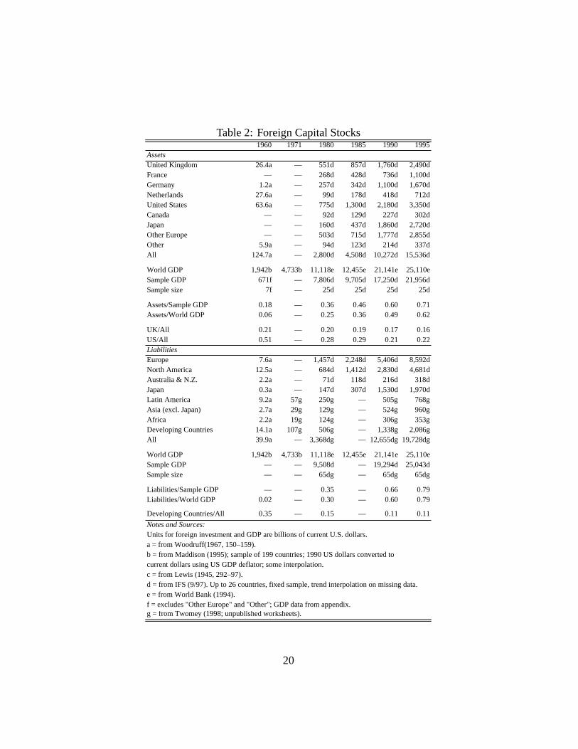
Table 2: Foreign Capital Stocks1960 1971 1980 1985 1990 1995

AssetsUnited Kingdom 26.4a — 551d 857d 1,760d 2,490dFrance — — 268d 428d 736d 1,100dGermany 1.2a — 257d 342d 1,100d 1,670dNetherlands 27.6a — 99d 178d 418d 712dUnited States 63.6a — 775d 1,300d 2,180d 3,350dCanada — — 92d 129d 227d 302dJapan — — 160d 437d 1,860d 2,720dOther Europe — — 503d 715d 1,777d 2,855dOther 5.9a — 94d 123d 214d 337dAll 124.7a — 2,800d 4,508d 10,272d 15,536d

World GDP 1,942b 4,733b 11,118e 12,455e 21,141e 25,110eSample GDP 671f — 7,806d 9,705d 17,250d 21,956dSample size 7f — 25d 25d 25d 25d

Assets/Sample GDP 0.18 — 0.36 0.46 0.60 0.71Assets/World GDP 0.06 — 0.25 0.36 0.49 0.62

UK/All 0.21 — 0.20 0.19 0.17 0.16US/All 0.51 — 0.28 0.29 0.21 0.22LiabilitiesEurope 7.6a — 1,457d 2,248d 5,406d 8,592dNorth America 12.5a — 684d 1,412d 2,830d 4,681dAustralia & N.Z. 2.2a — 71d 118d 216d 318dJapan 0.3a — 147d 307d 1,530d 1,970dLatin America 9.2a 57g 250g — 505g 768gAsia (excl. Japan) 2.7a 29g 129g — 524g 960gAfrica 2.2a 19g 124g — 306g 353gDeveloping Countries 14.1a 107g 506g — 1,338g 2,086gAll 39.9a — 3,368dg — 12,655dg 19,728dg

World GDP 1,942b 4,733b 11,118e 12,455e 21,141e 25,110eSample GDP — — 9,508d — 19,294d 25,043dSample size — — 65dg — 65dg 65dg

Liabilities/Sample GDP — — 0.35 — 0.66 0.79Liabilities/World GDP 0.02 — 0.30 — 0.60 0.79

Developing Countries/All 0.35 — 0.15 — 0.11 0.11

Notes and Sources:Units for foreign investment and GDP are billions of current U.S. dollars.a = from Woodruff(1967, 150–159).b = from Maddison (1995); sample of 199 countries; 1990 US dollars converted tocurrent dollars using US GDP deflator; some interpolation.c = from Lewis (1945, 292–97).d = from IFS (9/97). Up to 26 countries, fixed sample, trend interpolation on missing data.e = from World Bank (1994).f = excludes "Other Europe" and "Other"; GDP data from appendix.g = from Twomey (1998; unpublished worksheets).

20

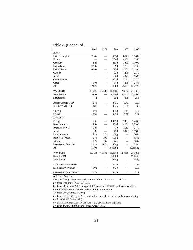
Table 2. (Continued)1960 1971 1980 1985 1990

AssetsUnited Kingdom 26.4a — 551d 857d 1,760dFrance — — 268d 428d 736dGermany 1.2a — 257d 342d 1,100dNetherlands 27.6a — 99d 178d 418dUnited States 63.6a — 775d 1,300d 2,180dCanada — — 92d 129d 227dJapan — — 160d 437d 1,860dOther Europe — — 503d 715d 1,777dOther 5.9a — 94d 123d 214dAll 124.7a — 2,800d 4,508d 10,272d

World GDP 1,942b 4,733b 11,118e 12,455e 21,141eSample GDP 671f — 7,806d 9,705d 17,250dSample size 7f — 25d 25d 25d

Assets/Sample GDP 0.18 — 0.36 0.46 0.60Assets/World GDP 0.06 — 0.25 0.36 0.49

UK/All 0.21 — 0.20 0.19 0.17US/All 0.51 — 0.28 0.29 0.21LiabilitiesEurope 7.6a — 1,457d 2,248d 5,406dNorth America 12.5a — 684d 1,412d 2,830dAustralia & N.Z. 2.2a — 71d 118d 216dJapan 0.3a — 147d 307d 1,530dLatin America 9.2a 57g 250g — 505gAsia (excl. Japan) 2.7a 29g 129g — 524gAfrica 2.2a 19g 124g — 306gDeveloping Countries 14.1a 107g 506g — 1,338gAll 39.9a — 3,368dg — 12,655dg

World GDP 1,942b 4,733b 11,118e 12,455e 21,141eSample GDP — — 9,508d — 19,294dSample size — — 65dg — 65dg

Liabilities/Sample GDP — — 0.35 — 0.66Liabilities/World GDP 0.02 — 0.30 — 0.60

Developing Countries/All 0.35 — 0.15 — 0.11

Notes and Sources:Units for foreign investment and GDP are billions of current U.S. dollars.a = from Woodruff(1967, 150–159).b = from Maddison (1995); sample of 199 countries; 1990 US dollars converted tocurrent dollars using US GDP deflator; some interpolation.c = from Lewis (1945, 292–97).d = from IFS (9/97). Up to 26 countries, fixed sample, trend interpolation on missing de = from World Bank (1994).f = excludes "Other Europe" and "Other"; GDP data from appendix.g = from Twomey (1998; unpublished worksheets).

21

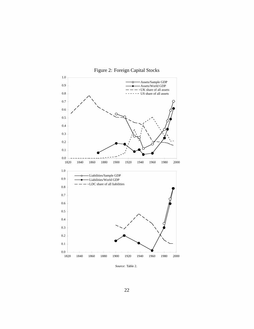
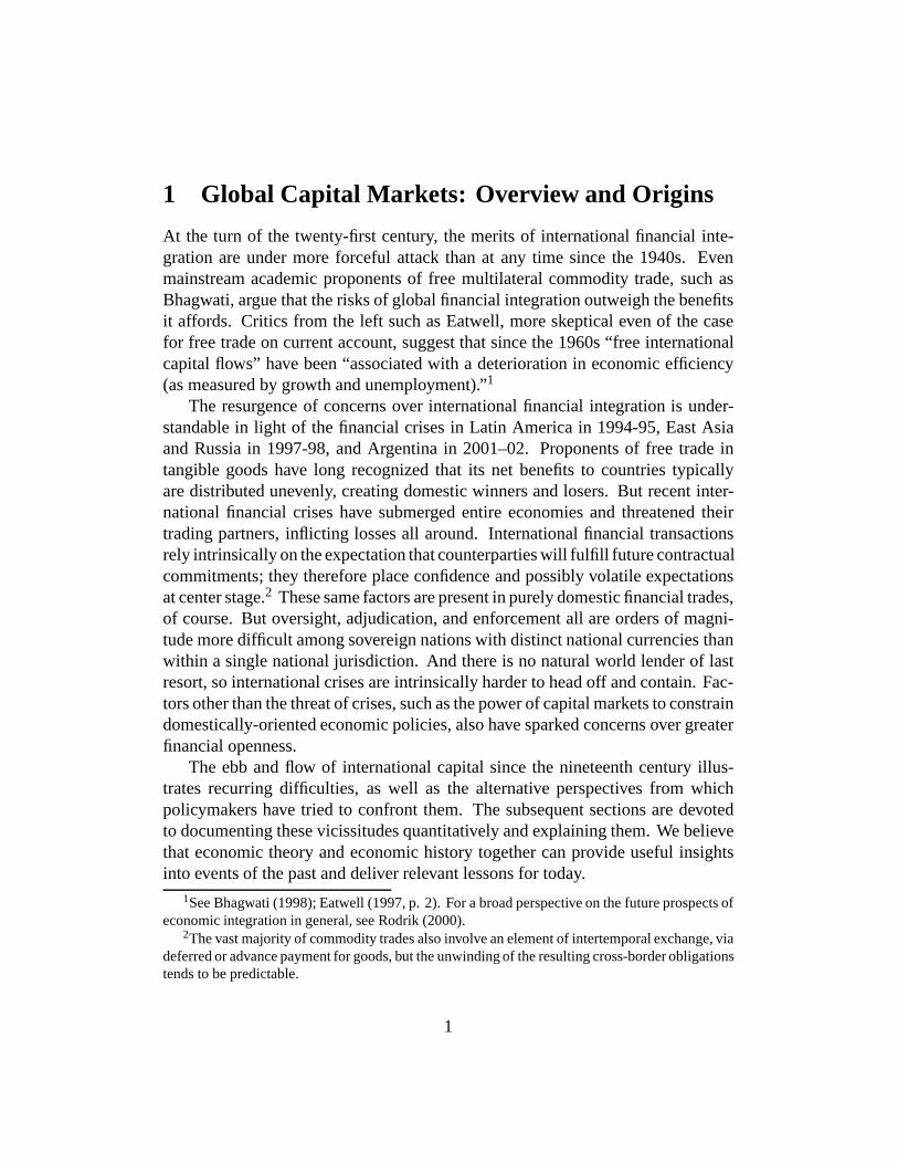
Figure 2: Foreign Capital Stocks

0.0

0.1

0.2

0.3

0.4

0.5

0.6

0.7

0.8

0.9

1.0

1820 1840 1860 1880 1900 1920 1940 1960 1980 2000

Assets/Sample GDPAssets/World GDPUK share of all assetsUS share of all assets

0.0

0.1

0.2

0.3

0.4

0.5

0.6

0.7

0.8

0.9

1.0

1820 1840 1860 1880 1900 1920 1940 1960 1980 2000

Liabilities/Sample GDPLiabilities/World GDPLDC share of all liabilities

Source: Table 2.

22

if not altogether willing, to assume the mantle of “banker to the world,” followingBritain’s abdication of this position under the burden of war and recovery in the1910s and 1920s.28 But the dislocations of the interwar years were to postpone theUnited States’ rise as a foreign creditor, and New York’s pivotal role as a financialcenter. After 1945, however, the United States decisively surpassed Britain as themajor international asset holder, a position that has never been challenged.29

How big were nineteenth century holdings of foreign assets? In 1870 weestimate that foreign assets were just 7 percent of World GDP; but this figure rosequickly, to just under 20 percent in the years 1900–14 at the zenith of the classicalgold standard. During the interwar period, the collapse was swift, and foreignassets were only 8 percent of world output by 1930, 11 percent in 1938, and just 5percent in 1945. Since this low point, the ratio has climbed, to 6 percent in 1960,25 percent in 1980, and then climbing dramatically to 62 percent in 1995. Thus,the 1900–14 ratio of foreign investment to output in the world economy was notequaled again until 1980, but has now been approximately doubled.

An alternative measure recognizes the incompleteness of the data sources: formany countries we have no information on foreign investments at all, so a zero hasbeen placed in the numerator, although that country’s output has been included inthe denominator as part of the World GDP estimate. This is an unfortunate aspectof our estimation procedure, and makes the above ratio a likely an underestimate, orlower bound, for the true ratio of foreign assets to output. One way to correct this isto only include in the denominator the countries for which we actually have data onforeign investment in the numerator.30 This procedure yields an estimate we termthe ratio of foreign assets to sample GDP. This is likely an overestimate, or upperbound, for the true ratio, largely because in historical data, if not in contemporarysources, attention in the collection of foreign investment data has usually focusedon the principal players, that is, the countries which have significant foreign assetholdings.31

28This Anglo-American transfer of hegemonic power is discussed by Kindleberger (1986) andby Bordo, Edelstein, and Rockoff (1999). Gallarotti (1995) challenges the view that Britain actedas a monetary hegemon up to 1914.

29Of course, this is the gross foreign investment position, not the net position. The United Statesis also now the world’s number one debtor nation, in both gross and net terms, having become anet debtor for the first time since the First World War in the late 1980s.

30That sample of countries is much less than the entire world, as we have noted. Until 1960, itincludes only the seven major creditor countries noted in Table 2; after 1980, we rely on the IMFsample from which we can identify up to 30 countries with foreign investment and GDP data.

31That is, we are probably restricted in these samples to countries with individually high ratios offoreign assets to GDP. For example, in the rest of Europe circa 1914, we would be unlikely to find

23

Given all these concerns, does the ratio to sample GDP evolve in a very differentway? No, but the recent upswing is not as pronounced using this alternativemeasure. The two ratios are very close after 1980. But before 1945 they are quitefar apart: from 1870 to 1914, the sample of seven countries has a foreign assetto GDP ratio of over 50 percent, far above the “world” fi gure of 7 to 20 percent.By this measure we only surpassed the 1914 ratio as recently as 1990, and onlynarrowly even then.

Clearly, these seven major creditors were exceptionally internationally diver-sified in the late nineteenth century in a way that no group of countries is today.By this reckoning, in countries like today’s United States, we still have yet to seea return to the extremely high degree of international portfolio diversification seenin, say, Britain in the 1900–14 period, an historical finding that places in historicalperspective the ongoing international diversification puzzle.32

Is the picture similar for liabilities as well as assets? Essentially, yes. Thedata are much more fragmentary here, with none in the nineteenth century, whenthe information for the key creditor nations was simpler to collect than data fora multitude of debtors, perhaps. Even so, we have some estimates running from1900 to the present at a few key dates. The ratio of liabilities to world GDP followsa path very much like that of the asset ratio, which is reassuring: they are eachapproximations built from different data sources at certain time points, though, inprinciple, they should be equal. Again, the ratio reaches a local maximum in 1914of 21 percent, collapsing in the interwar period to 11 percent in 1938, and just 2percent in 1960. By 1980 it had exceeded the 1914 level and stood at 30 percent.By 1995, the ratio was 79 percent.

To summarize, data on gross international asset positions seem broadly con-sistent with the idea of a ∪-shape in the evolution of international capital mobilitysince the late nineteenth century, though it is less clear how we should compare thedegree of diversification attained by some countries then with today’s apparentlysignificant, albeit declining, home bias in foreign asset holdings. Figuring whethertoo much or too little diversification existed at any point must remain conjectural,and conclusions would hinge on a calibrated and estimated portfolio model appliedhistorically. This is certainly an object for future research. However, unless theglobal economy has dramatically changed in terms of the risk-return profile of

countries with portfolios as diversified internationally as the British, French, Germans, and Dutch.If we included those other countries it would probably bring our estimated ratio down. However,in the 1980s and 1990s IMF data the problem is much less severe since we observe many morecountries, and both large and small asset holders.

32On the international diversification puzzle see K. Lewis (1999).

24

assets and their global distribution, we have no prior reason to expect the efficientdegree of diversification to have changed. For the present we can just say that,unless a massive such change did occur in the 1914–45 period, and unless it wasthen promptly reversed in the 1945–90 period, we cannot explain the time path offoreign capital stocks seen in Table 2 and Figure 2 except as a result of a dramaticdecline in capital mobility in the interwar period, and a very slow recovery ofcapital mobility thereafter.

There is another important dimension of international asset stock data that wehave not yet discussed: the evolution of net stocks, that is, the behavior of longer-term development flows, as distinct from diversification flows. The literature onthe Feldstein-Horioka (1980) paradox alerts us to the possibility that gross flowsare orders of magnitude above net flows. We postpone discussion of that issueuntil later.

2.2 Real Interest Rate Convergence

A fundamental property of fully integrated international capital markets is thatinvestors are indifferent on the margin between any two activities to which theyallocate capital, regardless of national location. International real interest rateequality would hold in the long run in a world where capital moves freely acrossborders and technological diffusion tends to drive a convergence process for na-tional production possibilities.33

One basic indication of internationally integrated financial markets thereforewould be the statistical stationarity of long-term real interest differentials. Weinvestigate this property using long-term real interest rate data constructed fromthe Global Financial Data database. For a nominal interest rate it we use themonthly series on long-term government bond yields, which apply to bonds ofmaturities of seven years or longer. For inflation πt = (Pt+12 − Pt)/Pt we usethe ex post 12-month forward rate of change of the consumer price index. The expost real interest rate is then calculated as rt = it − πt, and for now we make thestandard assumption that this is equal to the ex ante real rate plus a white-noisestationary forecast error. We focus on real long-term bond yields because these aremost directly related to financing costs for capital investments, and, hence, to the

33We focus on long-term real interest rates here because these rates are most closely linked tothe cost of long-lived capital, because the slow mean reversion in real exchange rates makes itdifficult to discern expected exchange rate changes in short-term data, and because risk premia canbe reduced over long horizons if long-run purchasing power parity holds.

25

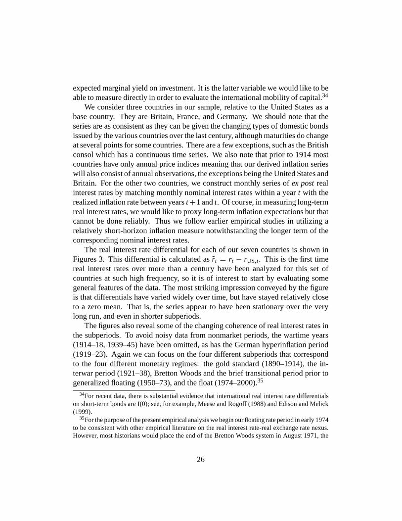
expected marginal yield on investment. It is the latter variable we would like to beable to measure directly in order to evaluate the international mobility of capital.34

We consider three countries in our sample, relative to the United States as abase country. They are Britain, France, and Germany. We should note that theseries are as consistent as they can be given the changing types of domestic bondsissued by the various countries over the last century, although maturities do changeat several points for some countries. There are a few exceptions, such as the Britishconsol which has a continuous time series. We also note that prior to 1914 mostcountries have only annual price indices meaning that our derived inflation serieswill also consist of annual observations, the exceptions being the United States andBritain. For the other two countries, we construct monthly series of ex post realinterest rates by matching monthly nominal interest rates within a year t with therealized inflation rate between years t+1 and t. Of course, in measuring long-termreal interest rates, we would like to proxy long-term inflation expectations but thatcannot be done reliably. Thus we follow earlier empirical studies in utilizing arelatively short-horizon inflation measure notwithstanding the longer term of thecorresponding nominal interest rates.

The real interest rate differential for each of our seven countries is shown inFigures 3. This differential is calculated as r̃t = rt − rUS,t. This is the first timereal interest rates over more than a century have been analyzed for this set ofcountries at such high frequency, so it is of interest to start by evaluating somegeneral features of the data. The most striking impression conveyed by the figureis that differentials have varied widely over time, but have stayed relatively closeto a zero mean. That is, the series appear to have been stationary over the verylong run, and even in shorter subperiods.

The figures also reveal some of the changing coherence of real interest rates inthe subperiods. To avoid noisy data from nonmarket periods, the wartime years(1914–18, 1939–45) have been omitted, as has the German hyperinflation period(1919–23). Again we can focus on the four different subperiods that correspondto the four different monetary regimes: the gold standard (1890–1914), the in-terwar period (1921–38), Bretton Woods and the brief transitional period prior togeneralized floating (1950–73), and the float (1974–2000).35

34For recent data, there is substantial evidence that international real interest rate differentialson short-term bonds are I(0); see, for example, Meese and Rogoff (1988) and Edison and Melick(1999).

35For the purpose of the present empirical analysis we begin our floating rate period in early 1974to be consistent with other empirical literature on the real interest rate-real exchange rate nexus.However, most historians would place the end of the Bretton Woods system in August 1971, the

26

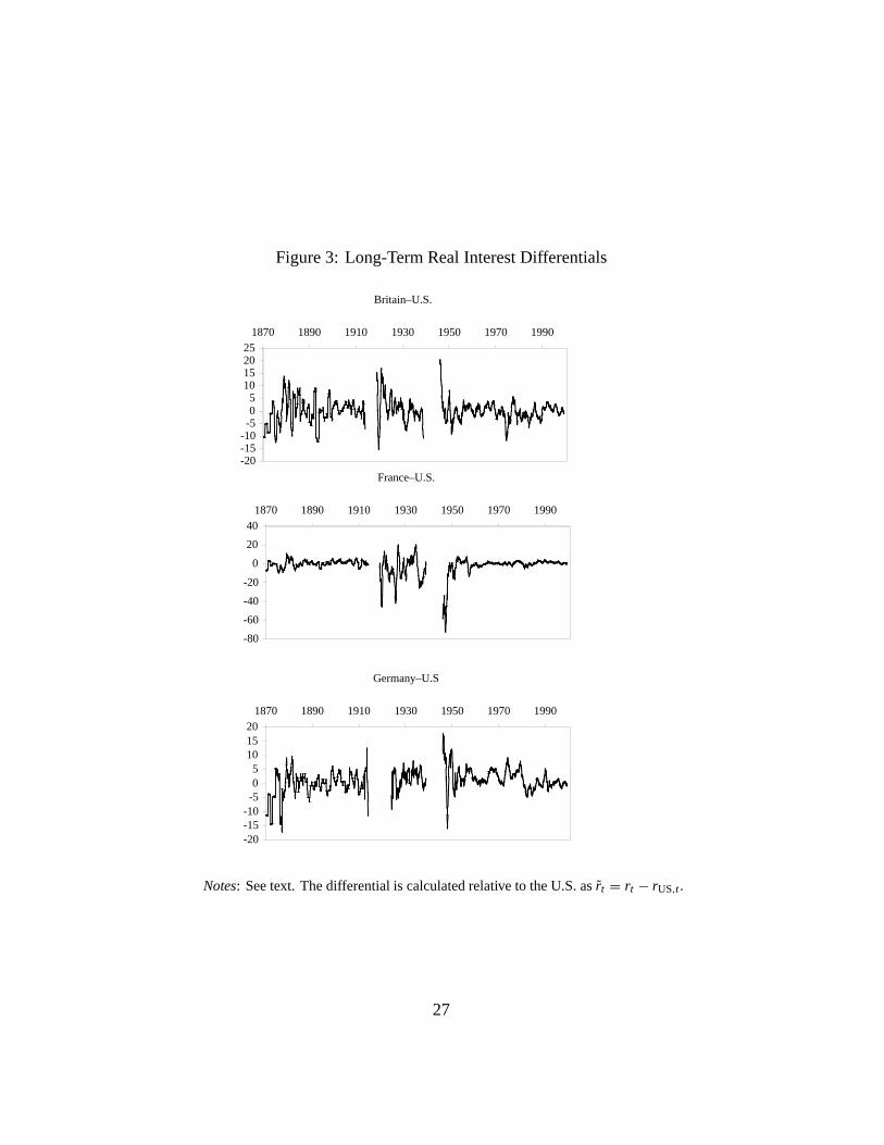
Figure 3: Long-Term Real Interest Differentials

Britain–U.S.

-20-15-10-505

10152025

1870 1890 1910 1930 1950 1970 1990

France–U.S.

-80

-60

-40

-20

0

20

401870 1890 1910 1930 1950 1970 1990

Germany–U.S

-20-15-10-505

101520

1870 1890 1910 1930 1950 1970 1990

Notes: See text. The differential is calculated relative to the U.S. as r̃t = rt − rUS,t .

27

Allowing for the annual inflation data used before 1914, we can see that realinterest differentials became somewhat more volatile in the interwar period, with alarger variance (this is less obvious in the German case because the hyperinflationperiod has been omitted). There is a decline in this volatility after 1950, andperhaps very little change between the pre-1974 period and the float. The latterobservation may seem surprising, except that it is consistent with observations that,aside from nominal and real exchange rate volatility, there is little difference in thebehavior of macro fundamentals between fixed and floating rate regimes, at leastfor developed countries (for example, Baxter and Stockman 1989).

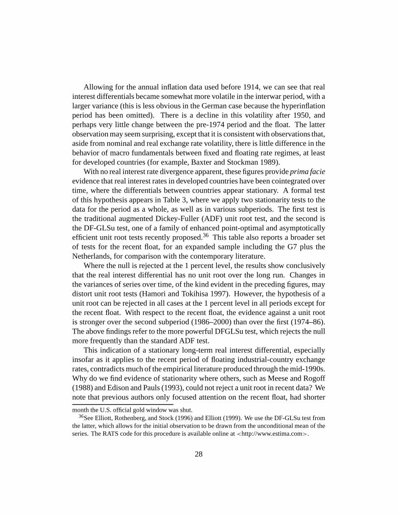
With no real interest rate divergence apparent, these figures provide prima facieevidence that real interest rates in developed countries have been cointegrated overtime, where the differentials between countries appear stationary. A formal testof this hypothesis appears in Table 3, where we apply two stationarity tests to thedata for the period as a whole, as well as in various subperiods. The first test isthe traditional augmented Dickey-Fuller (ADF) unit root test, and the second isthe DF-GLSu test, one of a family of enhanced point-optimal and asymptoticallyefficient unit root tests recently proposed.36 This table also reports a broader setof tests for the recent float, for an expanded sample including the G7 plus theNetherlands, for comparison with the contemporary literature.

Where the null is rejected at the 1 percent level, the results show conclusivelythat the real interest differential has no unit root over the long run. Changes inthe variances of series over time, of the kind evident in the preceding figures, maydistort unit root tests (Hamori and Tokihisa 1997). However, the hypothesis of aunit root can be rejected in all cases at the 1 percent level in all periods except forthe recent float. With respect to the recent float, the evidence against a unit rootis stronger over the second subperiod (1986–2000) than over the first (1974–86).The above findings refer to the more powerful DFGLSu test, which rejects the nullmore frequently than the standard ADF test.

This indication of a stationary long-term real interest differential, especiallyinsofar as it applies to the recent period of floating industrial-country exchangerates, contradicts much of the empirical literature produced through the mid-1990s.Why do we find evidence of stationarity where others, such as Meese and Rogoff(1988) and Edison and Pauls (1993), could not reject a unit root in recent data? Wenote that previous authors only focused attention on the recent float, had shorter

month the U.S. official gold window was shut.36See Elliott, Rothenberg, and Stock (1996) and Elliott (1999). We use the DF-GLSu test from

the latter, which allows for the initial observation to be drawn from the unconditional mean of theseries. The RATS code for this procedure is available online at <http://www.estima.com>.

28

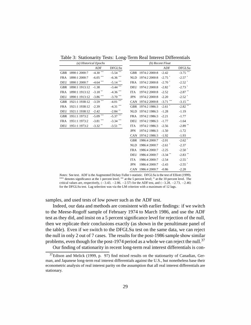
Table 3: Stationarity Tests: Long-Term Real Interest Differentials(a) Historical Epochs (b) Recent Float

ADF DFGLSu ADF DFGLSu

GBR 1890:1 2000:7 -4.30 *** -5.54 *** GBR 1974:2 2000:8 -2.42 -3.75 ***

FRA 1890:1 2000:7 -6.05 *** -6.36 *** NLD 1974:2 2000:8 -2.75 * -2.57 *

DEU 1890:1 2000:7 -4.64 *** -5.14 *** FRA 1974:2 2000:8 -2.70 * -2.52 *

GBR 1890:1 1913:12 -1.38 -3.44 *** DEU 1974:2 2000:8 -2.82 * -2.73 *

FRA 1890:1 1913:12 -3.18 ** -4.36 *** ITA 1974:2 2000:8 -2.52 -2.87 **

DEU 1890:1 1913:12 -3.86 *** -3.70 *** JPN 1974:2 2000:8 -2.20 -2.52 *

GBR 1921:1 1938:12 -3.59 *** -4.01 *** CAN 1974:2 2000:8 -3.71 *** -3.15 **

FRA 1921:1 1938:12 -2.39 -4.31 *** GBR 1974:2 1986:3 -2.61 * -2.82 **

DEU 1921:1 1938:12 -2.42 -2.84 ** NLD 1974:2 1986:3 -1.28 -1.19

GBR 1951:1 1973:2 -5.09 *** -5.37 *** FRA 1974:2 1986:3 -2.21 -1.77

FRA 1951:1 1973:2 -3.81 *** -3.34 *** DEU 1974:2 1986:3 -1.77 -1.64

DEU 1951:1 1973:2 -3.32 ** -3.51 *** ITA 1974:2 1986:3 -2.56 -2.89 **

JPN 1974:2 1986:3 -1.50 -1.72

CAN 1974:2 1986:3 -1.92 -1.93

GBR 1986:4 2000:7 -2.01 -2.62 *

NLD 1986:4 2000:7 -2.61 * -2.37

FRA 1986:4 2000:7 -2.25 -2.50 *

DEU 1986:4 2000:7 -3.34 ** -2.83 **

ITA 1986:4 2000:7 -2.54 -2.55 *

JPN 1986:4 2000:7 -2.43 -2.55 *

CAN 1986:4 2000:7 -0.86 -2.28

Notes: See text. ADF is the Augmented Dickey Fuller t-statistic. DFGLSu is the test of Elliott (1999).∗∗∗ denotes significance at the 1 percent level; ∗∗ at the 5 percent level; ∗ at the 10 percent level. Thecritical values are, respectively, (−3.43,−2.86,−2.57) for the ADF test, and (−3.28,−2.73,−2.46)for the DFGLSu test. Lag selection was via the LM criterion with a maximum of 12 lags.

samples, and used tests of low power such as the ADF test.Indeed, our data and methods are consistent with earlier findings: if we switch

to the Meese-Rogoff sample of February 1974 to March 1986, and use the ADFtest as they did, and insist on a 5 percent significance level for rejection of the null,then we replicate their conclusions exactly (as shown in the penultimate panel ofthe table). Even if we switch to the DFGLSu test on the same data, we can rejectthe null in only 2 out of 7 cases. The results for the post-1986 sample show similarproblems, even though for the post-1974 period as a whole we can reject the null.37

Our finding of stationarity in recent long-term real interest differentials is con-37Edison and Melick (1999, p. 97) find mixed results on the stationarity of Canadian, Ger-

man, and Japanese long-term real interest differentials against the U.S., but nonetheless base theireconometric analysis of real interest parity on the assumption that all real interest differentials arestationary.

29

sistent with another strand in the literature that does find support for internationalreal interest rate equalization at longer horizons (Fujii and Chinn 2000). We con-clude that earlier analyses of recent data were hampered by the low power of unitroot tests on samples of small span.38

2.3 Exchange-Risk Free Nominal Interest Parity

Perhaps the most unambiguous indicator of capital mobility is the relationship be-tween interest rates on identical assets located in different financial centers.39,40

The great advantage of comparing onshore and offshore interest rates such as theseis that relative rates of return are not affected by pure currency risk. For much of theperiod we study here, a direct onshore-offshore comparison is impossible. How-ever, the existence of forward exchange instruments allows us to construct roughlyequivalent measures of the return to currency-risk-free international arbitrage op-erations.

Using monthly data on forward exchange rates, spot rates, and nominal interestrates for 1921 to the latter half of 2001, we assess the degree of internationalfinancial-market integration by calculating the return to covered interest arbitragebetween financial centers. For example, a London resident could earn the grosssterling interest rate 1+ i∗t on a London loan of one pound sterling. Alternatively,she could invest the same currency unit in New York, simultaneously covering herexchange risk by selling dollars forward. She would do this in three steps: Buy et

38A more stringent test would examine the validity of long-term real interest parity. A focuson long-term real rather than nominal interest rate parity seems preferable because with meanreverting real exchange rates, it is easier to proxy long-run expected real exchange rates than thecorresponding nominal exchange rates. Meese and Rogoff (1988) rejected a version of real interestparity based on the maintained assumption of an underlying sticky-price exchange rate model.More supportive is the recent long-run panel cointegration study by MacDonald and Nagayasu(2000) of 14 OECD countries relative to the United States. The statistical methodology of thatwork, however, assumes that long-term real interest differentials are nonstationary. Chortareas andDriver (2001) implement a similar approach using a 17-country panel of OECD countries versusthe U.S.; their conclusions are similar to those of MacDonald and Nagayasu. Chortareas and Driverreport mixed results for tests on the stationarity of long-term real interest differentials. One issuepervading all of the work in this area is the effect of alternative proxies for long-term inflationexpectations. The proxies that are chosen often differ across authors, affecting some results. Asystematic discussion of these differences lies beyond the scope of this paper.

39See the discussion in Obstfeld (1995), for example.40This section draws heavily on Obstfeld and Taylor (1998) for the case of Britain, but adds

new data on Germany for comparison. After our 1998 paper was published, we became aware of asimilar 1889–1909 U.S.-U.K. interest rate comparison contained in Calomiris and Hubbard (1996).

30

dollars in the spot exchange market (where et is the spot price of sterling in dollarterms); next, invest the proceeds for a total of et(1 + it) (where it is the nominaldollar interest rate; and, finally, sell that sum of dollars forward for et(1 + it)/ftin sterling (where ft , the forward exchange rate, is the price of forward sterling interms of forward dollars). The net gain from borrowing in London and investingin New York,

et

ft(1+ it)− (1+ i∗t ), (3)

is zero when capital mobility is perfect and the interest rates and forward rate arefree of default risk. The left-hand side of the preceding expression represents aprice of present pounds sterling in terms of future pounds sterling, i.e., of poundsdated t in terms of pounds dated t + 1, but it can be viewed as the relative priceprevailing in the New York market, that is, as a kind of offshore interest rate. Thus,our test, in effect, examines the equality of the onshore sterling interest rate i∗with the offshore New York rate so defined. We perform a similar calculation formark interest differentials between London (considered as the offshore center) andGermany (onshore), thereby gauging the difference between implicit mark interestrates in London and the rates prevailing near the same time in Germany.

For pre-1920 data, we examine a related but distinct measure based on currentNew York prices of sterling for (two-months) future delivery, as in Obstfeld andTaylor (1998). The parallel Germany-London arbitrage calculation before 1920,corresponding to the preceding New York-London comparison, is based on Londonprices for marks to be delivered three months in the future. Forward exchangecontracts of the kind common after 1920 were not prevalent before then (except insome exceptional financial centers, see Einzig 1937), so we instead base our pre-1920 comparison of onshore and offshore interest rates on the most widely tradedinstrument, one for which prices were regularly quoted in the major financialcenters’ markets, the long bill of exchange. Long bills could be used to cover theexchange risk that might otherwise be involved in interest-rate arbitrage.41

To see how such a transaction would work, let bt denote the date-t dollar pricein New York of £1 deliverable in London after 60 days, and et the spot New Yorkprice of sterling.42 One way to purchase a future pound deliverable in Londonwould be through a straight sterling loan, at price 1/(1 + i∗t ), where i∗t is theLondon 60-day discount rate. An alternative would be to purchase in New York

41Margraff (1908, p. 37) speaks explicitly of the need to “cover” interest arbitrage through theexchange market.

42In fact such bills were payable after 63 days due to a legal “grace period” of three days, aninstitutional fact we account for in the calculations below (Haupt 1894, p. 429).

31

a bill on London, at a price in terms of current sterling of bt/et . With perfect andcostless international arbitrage, these two prices of £1 to be delivered in Londonin the future should be the same.

Perkins (1978) observed that the series (e/b) − 1 defines the sterling interestrate in American financial markets, that is, the offshore sterling rate in the UnitedStates. This series may be compared with the London rate i∗, as we did in our1998 paper, to gauge the degree of cross-border financial integration; that is, wecalculate the differential et

bt− (1+ i∗t )

before 1920.Perkins’s (1978) primary aim was to modify earlier series of dollar-sterling

spot rates derived by Davis and Hughes (1960), who applied U.S. rather than U.K.interest rates to the dollar prices of long sterling bills in order to infer a series ofsight exchange rates. Perkins argued that the sight bill rate should be derived bymultiplying the (lower) long bill rate by a sterling, not a dollar, interest factor, andsubsequent scholars have followed him; see, for example, the judgment of Officer(1996, p. 69). From a theoretical point of view, the verdict is clear: the relativeprice of current and future sterling defines a sterling nominal interest rate, in thepresent case, the offshore New York rate that we compare to London rates.

The upper panel of Figure 4 is based on monthly differences between sterlingrates in New York and in London from 1870 to 2001, where we simply splicetogether the 1870–1919 numbers based on time bill rates with the subsequentlyavailable covered interest differentials. Differential returns are calculated as annualrates of accrual.43

43The U.S.-U.K. comparison is based on the data described in Obstfeld and Tayor (1998, p. 361,n. 7), with the following amendments. From January 1975-August 2001, the London sterling inter-est rate i∗ is the three-month bank bill middle rate, from Datastream. From January 1981-August2001, the New York dollar interest rate i is the discount rate on 90-day bankers’ acceptances, fromDatastream. Finally, from January 1981-August 2001 spot and three-month forward dollar-sterlingexchange rates come from Datastream. All of these new data are end-of-month observations.

For the U.K.-German comparison, data are monthly averages up until January 1981 and endof month thereafter, as follows. Exchange rates: From October 1877 to July 1914 we use themonth-average spot mark-sterling exchange rate from the NBER macro-history database, series14106 (hereafter “NBER” ). London sterling prices for three-month bills on Berlin are “money”rates taken from the “Course of Exchange” table in the Economist. From January 1921-September1931 we average the weekly spot and three-month forward exchange rates listed by Einzig (1937).From May 1955 to December 1980, spot exchange rates are from the Economist through 1957and thereafter from Datastream. Forward exchange rates are from the London Times (May 1955-October 1958), from the Economist subsequently through 1964, then from the London Times

32

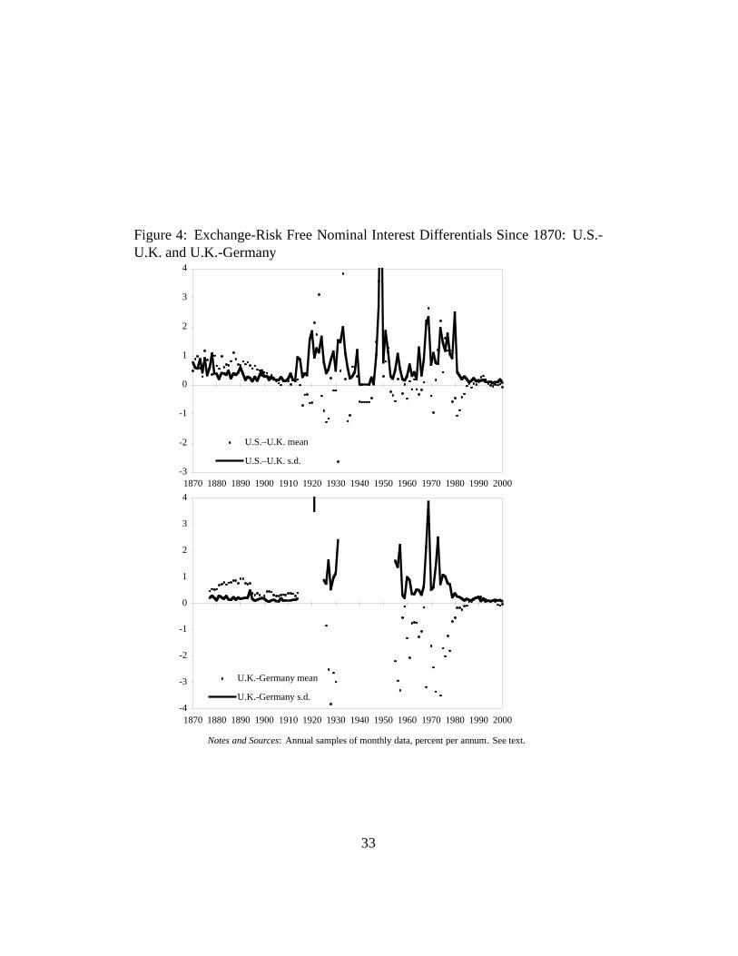
Figure 4: Exchange-Risk Free Nominal Interest Differentials Since 1870: U.S.-U.K. and U.K.-Germany

-3

-2

-1

0

1

2

3

4

1870 1880 1890 1900 1910 1920 1930 1940 1950 1960 1970 1980 1990 2000

U.S.–U.K. mean

U.S.–U.K. s.d.

-4

-3

-2

-1

0

1

2

3

4

1870 1880 1890 1900 1910 1920 1930 1940 1950 1960 1970 1980 1990 2000

U.K.-Germany mean

U.K.-Germany s.d.

Notes and Sources: Annual samples of monthly data, percent per annum. See text.

33

The figure broadly supports other indicators of the evolution of capital mobility.Differentials are relatively small and steady under the pre-1914 gold standard, butstart to open up during World War I. They stay quite large in the early 1920s.Differentials diminish briefly in the late 1920s, but widen sharply in the early1930s. There are some big arbitrage gaps in the late 1940s through the mid-1950s—including a sharp spike in volatility at the time of the 1956 Suez crisis.44

But these shrink starting in the late 1950s and early 1960s, only to open up again inthe late 1960s as sterling’s 1967 devaluation initiates a period of foreign exchangeturmoil, culminating in the unraveling of the Bretton Woods system in the early1970s. Interest differentials have become small once again since the disappearanceof U.K. capital controls around 1980. The differentials appear even smaller nowthan before 1914.45

Indeed, for the 1870–1914 data we observe a tendency, quite systematic albeitdeclining over time, for New York sterling rates to exceed London rates. In arguingin favor of a sterling discount rate for valuing long sterling bills traded in the U.S.,Perkins (1978) demonstrated a tendency for the implicit offshore sterling interestrate (e/b) − 1 to converge toward Bank Rate toward the end of the nineteenthcentury (see his Figure 2, p. 399). Our Figure 4, however, compares the New York

through 1975, and, finally, starting January 1976, from Datastream. U.K. three-month interest rate:Open market three-month discount rate, NBER series 13016, through September 1931. Data from1955–74 come from the Federal Reserve banking data base (and are similar to the well-knownCapie-Webber series). Starting in January 1975 we use the U.K. interbank (money-market) three-month middle rate of interest. German three-month interest rate: From October 1877 throughSeptember 1931, where observations are available, we use the Berlin private open market discountrate for prime bankers’ acceptances given as NBER series 13018. The German three-month moneymarket rate for 1955–59 is an average of monthly high and low rates taken from Monthly Report ofthe Deutsche Bundesbank and thereafter, through end-1980, comes from International FinancialStatistics. Subsequent data are from Datastream, the three-month “dead middle” money marketrate.

44See Klug and Smith (1999) for a fascinating empirical study of the Suez crisis. The paperincludes a discussion of daily covered arbitrage differentials from June 1, 1956—January 31, 1957.

45We alert the reader to several potential problems with our calculations and data. First, as wehave stressed already above and indeed stressed quite clearly in Obstfeld and Taylor (1998), the twomeasures of market integration that we calculate refer to different arbitrage possibilities before andafter 1920. Second, some forward transactions appear at different maturities in our data set. Third,most data are observed at or near end-of-month, but some data are averages of weekly numbers.Averaging has the effect of dampening measured volatility. Fourth, data from World War II reflectrigidly administered prices and have no capital-mobility implications. Fifth, the data used are notclosely aligned for time of day (and even differ as to day in some cases), so that some deviationsfrom parity may be exaggerated. The purpose of the exercise, however, is merely to convey a broadsense of the trend in integration, not to pursue a detailed hunt for small arbitrage possibilities.

34

offshore sterling interest rate with the London money-market rate of discount,which tended to be somewhat below Bank Rate. Were we to use Bank Rate as theLondon interest rate in the figure, much of the pre-1914 gap would be eliminated.Given that the U.S. data consist of prices of high quality paper (such as bank bills),however, comparisons with Bank Rate are probably inappropriate. As Spalding(1915, p. 49) observes: “Bank Rate, as is well known, is usually higher than marketrate; therefore if ordinary trade bills are remitted [to London] from [abroad], tofind the long exchange, interest will be calculated at our Bank Rate, as trade paperis not considered such a good security as bank bills.”46 Officer (1996, p. 69)concurs, though on different grounds: “Whereas the Bank Rate was set by theBank of England, the money-market rate was a true competitive price …. Themoney-market rate of discount is the better measure ….”

If it is impermissible to compare the sterling interest rate in New York withBank Rate in London, how, then, can we explain the systematic positive interestgap in favor of New York before 1914? Much if not all of the gap can be explainedas an artifact of the procedure we have used to extract the “offshore” interest ratefrom the observations on sight and time bill prices.

Continuing our focus on the New York-London comparison of sterling interestrates, we notice that the published money-market discount rate for London isquoted as a “pure” relative price of future in terms of present sterling. In contrast,as practitioners’ textbooks of the period make amply clear, in determining the priceto be paid for a long bill of exchange on London, purchasers would factor in notonly the spot exchange rate and the London market discount rate, but, in addition,commissions, profit margins, and, importantly, the stamp duty (0.05 percent of thebill’s face value) payable to the British government. These factors made bill priceslower than they would have been if they simply were equal to the spot exchangerate discounted by the pure New York sterling rate of interest.

Margraff (1908, p. 121) estimates that for a 90-day bill, the total of suchfactors amounted to 0.125 percent of face value. For a 60-day bill, that chargewould represent about 75 basis points in annualized form; Escher (1918, pp. 81–2), published a decade later, cites a very slightly smaller number. By subtractingthat “ tax” from the pre-1914 differentials plotted in the top of Figure 4, we see thatthe apparent average excess return in New York disappears.

Indeed, the average return becomes negative for 1890–1914, so that 75 basispoints in additional costs may well be an overestimate for the entire prewar period.Suggestive of declining costs is the tendency shown in the figure for the average

46See also the summary table in Margraff (1908, p. 112).

35

bias to decline over time. Perkins (1978, pp. 400–1) argues that U.S. foreignexchange dealers of the period were able to exploit market power to inflate theircommissions. Certainly such market power declined through 1914 as marketsevolved, and Officer’s (1996, p. 75) data on brokers’ commissions supports thisview.47 Of course, a process of market integration increases competition and drivescommissions down. Thus, leaving aside the portion due to the stamp tax, the sizeof the New York-London discrepancy is to some degree a reflection of financialmarket segmentation and its secular decline evidence of a process of progressiveintegration.

The lower panel of Figure 4 shows the difference between the implicit markinterest rate in London and the one prevailing in Germany. Before 1914, the former,offshore, rate is calculated on the basis of 90-day prime bills of exchange on Berlintraded in London. The results are remarkably consistent with those for New York-London. In particular, we again observe a systematic but secularly declining excessreturn in London prior to 1914.

The explanation is essentially the same as in the New York-London comparisonabove. Germany levied a stamp duty on bills at the same rate as Britain’s (0.05percent; see Haupt 1894, p. 164, or Margraff 1908, p. 133). Margraff’s estimatesof concomitant costs suggest that for a 90-day bill on Berlin, about 40 basis pointsshould be subtracted from the annualized sight bill premium 4 × [(e/b) − 1] toascertain the true London mark interest rate. On the assumption that some costsdecline over time, with 40 basis points an average for the prewar period as whole,that cost adjustment brings the offshore and onshore mark rates roughly into line.48

While the cost and tax considerations we have described potentially eliminatethe upward bias in our estimated series of offshore interest rates, other financialtransaction costs would, as usual, create no-arbitrage bands around the point ofonshore-offshore interest rate equality. One way to evaluate the evolution of capitalmobility through time would be to estimate over different eras what Einzig (1937,p.25) calls “ transfer points,” i.e., the minimum return differential necessary to inducearbitrage operations. Keynes and Einzig agreed that during the interwar period, at

47Country risk type arguments cannot easily rationalize the pre-1920 interest differential in favorof New York, as we pointed out earlier in Obstfeld and Taylor (1998, p. 361, n. 6). The reason isthat the two transactions we compare both entail future payment in the same place, London. Thisis not the case in the post-1920 covered interest arbitrage calculations.

48Flandreau and Rivière (1999) focus on a London-Paris comparison. Their results are entirelyconsistent with the data that we show in Figure 4, including a systematic excess of the Londonfranc interest rate over that in Paris. Their rationale for the differential is apparently different fromours, although they do not include details of their derivation.

36

least a 50 basis point covered differential would be needed to induce arbitrage. Thatis, they suggested a no-arbitrage band of ±50 basis points. Applying nonlinearestimation techniques including a TAR methodology to weekly interwar data ondollar-sterling covered return differentials, Peel and Taylor (2002) confirm that ano-arbitrage band close to ±50 basis points did appear to prevail, as Keynes andEinzig claimed. Only outside of this range did arbitrage forces push spot andforward exchange rates toward conformity with the band.

A detailed investigation is beyond the scope of this paper, but a first passat the data using the TAR methodology described earlier is suggestive. For thedollar-sterling exchange between June 1925 and June 1931, we calculate a band ofinaction of ±60 basis points, very close to the Peel-Taylor estimate given that weare using coarser, monthly data. For the corresponding interwar sterling-mark ex-change our estimated band is ±91 basis points wide. On 1880–1914 differentials,in contrast, we find (after subtracting a constant mean differential) bands of only±19 basis points for New York-London and ±35 basis points for London-Berlin.By way of comparison, Clinton (1988) suggests that covered interest differentialsin the mid-1980s needed to reach just ±6 basis points to become economicallysignificant, and the bar is certainly even lower by now. We suspect that a morecareful analysis of pre-1914 differentials, one taking account of the upward trend inmarket integration, would reduce our estimated transaction cost bands for the earlytwentieth century. Accordingly, the degree of integration among core money mar-kets achieved under the classical gold standard must be judged as truly impressivecompared to conditions over the following half century or so.

The Great Depression, perhaps as part of a much broader interwar phase ofdisintegration, therefore stands out as an event that transformed the world capitalmarket and left interest arbitrage differentials higher and more volatile than everbefore.

2.4 Equity and Bond Returns

It is interesting to ask whether the long-run evidence on the ∪-shape of capitalmarket integration extends to other criteria, and other markets such as equities.Over the long run, global equity markets have evolved at a very different rate thanglobal bond markets, for example. Government bonds from core countries havegenerally traded in financial centers in the last one hundred years, but for long spansof time emerging-market debt was very difficult to place in the private sector, andmost went through multilateral intermediaries. Similarly, international trade inequities, though quiescent in the middle of the century, grew substantially in core

37

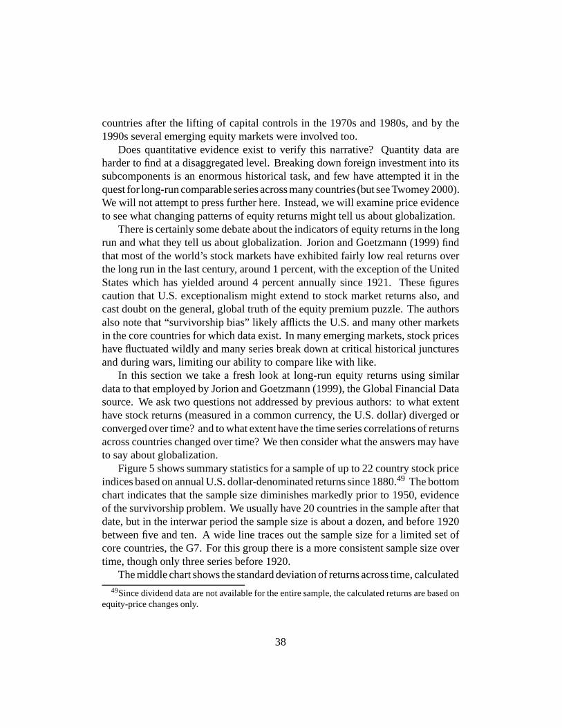
countries after the lifting of capital controls in the 1970s and 1980s, and by the1990s several emerging equity markets were involved too.

Does quantitative evidence exist to verify this narrative? Quantity data areharder to find at a disaggregated level. Breaking down foreign investment into itssubcomponents is an enormous historical task, and few have attempted it in thequest for long-run comparable series across many countries (but see Twomey 2000).We will not attempt to press further here. Instead, we will examine price evidenceto see what changing patterns of equity returns might tell us about globalization.

There is certainly some debate about the indicators of equity returns in the longrun and what they tell us about globalization. Jorion and Goetzmann (1999) findthat most of the world’s stock markets have exhibited fairly low real returns overthe long run in the last century, around 1 percent, with the exception of the UnitedStates which has yielded around 4 percent annually since 1921. These figurescaution that U.S. exceptionalism might extend to stock market returns also, andcast doubt on the general, global truth of the equity premium puzzle. The authorsalso note that “survivorship bias” likely afflicts the U.S. and many other marketsin the core countries for which data exist. In many emerging markets, stock priceshave fluctuated wildly and many series break down at critical historical juncturesand during wars, limiting our ability to compare like with like.

In this section we take a fresh look at long-run equity returns using similardata to that employed by Jorion and Goetzmann (1999), the Global Financial Datasource. We ask two questions not addressed by previous authors: to what extenthave stock returns (measured in a common currency, the U.S. dollar) diverged orconverged over time? and to what extent have the time series correlations of returnsacross countries changed over time? We then consider what the answers may haveto say about globalization.

Figure 5 shows summary statistics for a sample of up to 22 country stock priceindices based on annual U.S. dollar-denominated returns since 1880.49 The bottomchart indicates that the sample size diminishes markedly prior to 1950, evidenceof the survivorship problem. We usually have 20 countries in the sample after thatdate, but in the interwar period the sample size is about a dozen, and before 1920between five and ten. A wide line traces out the sample size for a limited set ofcore countries, the G7. For this group there is a more consistent sample size overtime, though only three series before 1920.

The middle chart shows the standard deviation of returns across time, calculated49Since dividend data are not available for the entire sample, the calculated returns are based on

equity-price changes only.

38

Figure 5: Equity Returns in U.S. Dollars for the G7 and up to 22 Global StockMarkets, 1880–2000

sample size

0

5

10

15

20

25

1880 1900 1920 1940 1960 1980 2000

s.d. (10 year window)

0.0

0.1

0.2

0.3

0.4

0.5

1880 1900 1920 1940 1960 1980 2000

correlations (10 year window)

-0.5

0.0

0.5

1.0

1880 1900 1920 1940 1960 1980 2000

Source: Global Financial Data.

39

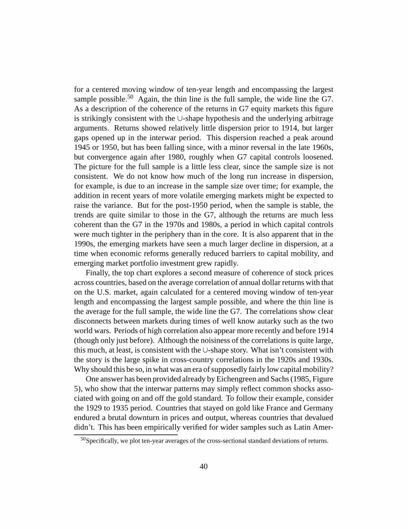
for a centered moving window of ten-year length and encompassing the largestsample possible.50 Again, the thin line is the full sample, the wide line the G7.As a description of the coherence of the returns in G7 equity markets this figureis strikingly consistent with the ∪-shape hypothesis and the underlying arbitragearguments. Returns showed relatively little dispersion prior to 1914, but largergaps opened up in the interwar period. This dispersion reached a peak around1945 or 1950, but has been falling since, with a minor reversal in the late 1960s,but convergence again after 1980, roughly when G7 capital controls loosened.The picture for the full sample is a little less clear, since the sample size is notconsistent. We do not know how much of the long run increase in dispersion,for example, is due to an increase in the sample size over time; for example, theaddition in recent years of more volatile emerging markets might be expected toraise the variance. But for the post-1950 period, when the sample is stable, thetrends are quite similar to those in the G7, although the returns are much lesscoherent than the G7 in the 1970s and 1980s, a period in which capital controlswere much tighter in the periphery than in the core. It is also apparent that in the1990s, the emerging markets have seen a much larger decline in dispersion, at atime when economic reforms generally reduced barriers to capital mobility, andemerging market portfolio investment grew rapidly.

Finally, the top chart explores a second measure of coherence of stock pricesacross countries, based on the average correlation of annual dollar returns with thaton the U.S. market, again calculated for a centered moving window of ten-yearlength and encompassing the largest sample possible, and where the thin line isthe average for the full sample, the wide line the G7. The correlations show cleardisconnects between markets during times of well know autarky such as the twoworld wars. Periods of high correlation also appear more recently and before 1914(though only just before). Although the noisiness of the correlations is quite large,this much, at least, is consistent with the ∪-shape story. What isn’ t consistent withthe story is the large spike in cross-country correlations in the 1920s and 1930s.Why should this be so, in what was an era of supposedly fairly low capital mobility?

One answer has been provided already by Eichengreen and Sachs (1985, Figure5), who show that the interwar patterns may simply reflect common shocks asso-ciated with going on and off the gold standard. To follow their example, considerthe 1929 to 1935 period. Countries that stayed on gold like France and Germanyendured a brutal downturn in prices and output, whereas countries that devalueddidn’ t. This has been empirically verified for wider samples such as Latin Amer-

50Specifically, we plot ten-year averages of the cross-sectional standard deviations of returns.

40

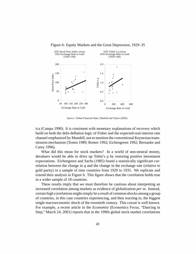
Figure 6: Equity Markets and the Great Depression, 1929–35

1935 Stock Price Index versus 1935 Exchange Rate to Gold

(1929=100)

0

50

100

150

200

50 100 150 200 250 300

Exchange Rate to Gold

Stoc

k Pr

ice

Inde

x1935 Tobin’s q versus

1935 Exchange Rate to Gold (1929=100)

0.0

0.5

1.0

1.5

2.0

0 200 400 600

Exchange Rate to Gold

Tob

in’s

q

Source: Global Financial Data; Obstfeld and Taylor (2002).

ica (Campa 1990). It is consistent with monetary explanations of recovery whichbuild on both the debt-deflation logic of Fisher and the expected-real-interest-ratechannel emphasized by Mundell, not to mention the conventional Keynesian trans-mission mechanism (Temin 1989; Romer 1992; Eichengreen 1992; Bernanke andCarey 1996).

What did this mean for stock markets? In a world of non-neutral money,devaluers would be able to drive up Tobin’s q by restoring positive investmentexpectations. Eichengreen and Sachs (1985) found a statistically significant cor-relation between the change in q and the change in the exchange rate (relative togold parity) in a sample of nine countries from 1929 to 1935. We replicate andextend their analysis in Figure 6. This figure shows that the correlation holds truein a wider sample of 18 countries.

These results imply that we must therefore be cautious about interpreting anincreased correlation among markets as evidence of globalization per se. Instead,certain high correlations might simply be a result of common shocks among a groupof countries, in this case countries experiencing, and then reacting to, the biggestsingle macroeconomic shock of the twentieth century. This caveat is well known.For example, a recent article in the Economist (Economics Focus, “Dancing inStep,” March 24, 2001) reports that in the 1990s global stock market correlations

41

have risen to even higher levels than in the late 1980s (as high as 0.8 in year2000, though at what frequency is not mentioned).51 This came after a declinein correlations in the early 1990s, but “ the long term trend is upward.” Overall,the article concludes, this is consistent with increased globalization pressures, butcertain large shocks, like the recent crises in Asia, might also have also beenassociated with higher correlations via contagion channels. As the article notes,“stock markets tend to be more correlated at times of high volatility in shareprices; during calmer periods, correlations tend to be weaker.” Similar reasoning,of course, could pertain to the roaring twenties, and the bust of the thirties.52

2.5 Summary

Many studies of market integration have focused on a single kind of criterion.This approach seems unreasonably restrictive to us, since the interpretation ofsuch narrow criteria must necessarily rest upon untested auxiliary assumptions.By contrast, we see no reason to dismiss any useful information, in either price orquantity form, especially given the paucity of historical data in certain quarters.Thus, we have opted for a broad battery of tests to try to cut down the possible setof explanations that could account for the empirical record, and so, by a process ofelimination, work towards a set on controlled conjectures concerning the evolutionof the global capital market.

The preceding section succinctly conveys the benefits we think this kind ofapproach can deliver. Our quantity-based tests delivered a certain set of stylizedfacts, and the price-based tests another set of facts. Combining the two, andintroducing evidence on convergence and divergence in other economic phenomenasuch as living standards and demography, we claim there is overwhelming supportfor the notion that the major long-run changes in the degree of global capitalmobility have taken the form of changes in the impediments to capital flows, ratherthan any encouragement or discouragement to flows arising from structural shiftswithin the economies themselves. That is not to discount the fact that such changeshave occurred, and are no doubt important at the margin; but it is an assertion thatthe virtual disappearance of foreign capital flows and stocks in mid-century, and

51On these correlations see also Gourinchas and Rey (2001) and International Monetary Fund(2001, p. 76).

52The definition of “contagion” is controversial: contagion may entail a structural intensificationof spillovers in crisis periods. As Forbes and Rigobon (2000) stress, however, higher return volatilityitself can mechanically raise cross-border return correlations even in the absence of any underlyingstructural change, and it may be misleading to view this as a contagion effect.

42

the explosion in price differentials, can only be explained by an appeal to changesin arbitrage possibilities as permitted by two major constraining factors in capitalmarket operations: technology and national economic policies.

From this point, it is a short step to the conclusion that a full accounting ofthe phenomena at hand must rest on a detailed political and institutional history.Clearly, technology is a poor candidate for the explanation of the twentieth cen-tury collapse of capital mobility. In the 1920s and 1930s the prevailing financialtechnologies were not suddenly forgotten by market participants: indeed sometechnologies, such as futures markets for foreign exchange came to fruition inthose decades. Technological evolution was not smooth and linear, but, as wehave already noted, was at least unidirectional, and, absent any other impediments,would have implied an uninterrupted progress toward an ever more tightly con-nected global marketplace.

Such was not allowed to happen, of course. Rather, the shifting forces ofnational economic policies, as influenced by the prevailing economic theories ofthe day, loomed large during and after the watershed event of the twentieth century,the economic and political crisis of the Great Depression. Understanding themacroeconomic and international economic history of the last century in theseterms, and the changes it wrought for the operation of the global capital market,is a long and complex story, a narrative that properly accompanies the empiricalrecord presented in this paper, and we take up some of the political economydimensions of that story in the section that follows.

3 Political Economy

We have thus far amassed some evidence that international capital mobility has ex-perienced two major swings over the course of the twentieth century: a pronounceddecline during the interwar years and a recovery in the later postwar years. Thetiming is hard to pin down precisely, and, indeed, surely varied by country and bythe type of capital movements being considered.

Taking this as given, we now must ask, why did capital mobility follow thispath, and what corroborative evidence can we assemble to buttress an account ofthese events that incorporates the forces of political economy? We start first withthe downturn in capital mobility after 1914.

43

3.1 The Downturn

The conventional macro-historical account of the collapse of capital mobility after1914 focuses on the trilemma, as we have noted (Eichengreen 1996; Obstfeldand Taylor 1998). The literature suggests that the major political economy forcesat work during this period were increasing pressure for macroeconomic activism,particularly from newly- or better-enfranchised groups such as the working classes.If fixed exchange rates were to be maintained, then capital mobility would have to becompromised, at least on some occasions. Maintenance of capital mobility insteadwould preclude an exchange rate target. Either option would raise uncertainty forinvestors.

It is believed that prior to 1914, gold standard orthodoxy had been a sine quanon for access to global capital markets on favorable terms. A first study Bordoand Rockoff (1996) found that adherence to gold standard rules acted as a “sealof approval” for sovereign debt. Gold standard countries had lower country risk,measured by the bond spread in London over the British consol.53 Accordingly,evidence of a new political dynamic after 1914 might be seen in a changing rela-tionship between country risk and gold after the gold standard was reconstitutedstarting in 1925. With the rules of the game in question after World War I, investorsmight have doubted whether the announcement of a gold standard commitmentalone would signal credibility. In addition, public solvency indicators, such asdebt-GDP ratios, or inflation, might be seen as having a bigger impact on inter-national bond spreads under the reconstituted gold standard than before. Do suchdoubts manifest themselves in the data?

There is no uniform and comprehensive study of bond spreads across thesetwo eras that would allow us definitively to answer this question, but a secondstudy by Bordo, Edelstein, and Rockoff (1999) came to a conclusion that wassurprising, even by the authors’ own admission. Looking solely at 1920s bondsthey found continued evidence that the gold standard remained a seal of approval,lowering bond spreads significantly, at least when a country stuck to its prewarparity. Devaluers were not so lucky with their bond spreads, since for them, theimpact of being on gold was small and statistically insignificant. Such a conclusionchallenged the conventional wisdom that the interwar gold standard was a pale andless credible shadow of its predecessor.

These are two pioneering studies but, for comparative work across regimes,53Clemens and Williamson (2001), however, find no statistically significant gold standard effect

on the shares of British capital flows to various foreign recipients during 1870–1913. It remains toreconcile the apparently conflicting message of the price and quantity data.

44

they are not ideal. Unfortunately, they cannot be merged together into a consistentpicture because of differences in the methods and data employed. The former studylooked at long-term government bonds in the secondary market, and examined theiryield to maturity; the latter examined new issues and their yield at the moment offlotation only. The former study therefore had complete time series, whereas thelatter had a small sample that was often interrupted by missing data in years whenno issues took place—a not uncommon event in the 1920s, and one that could raisea potential sample-selection issue. Finally, the former studied prices in London,the latter prices in New York, a switch that could be defended as the hegemoniccenter of global capital markets shifted across the Atlantic around this time, andone that allowed the use of Cleona Lewis’ (1938) data on new issues for the 1920s.

To overcome the differences between these studies, we re-examine the questionof what determined bond spreads in the pre-1914 and interwar years using a muchlarger database that allows us to view a consistent set of data for a larger sampleof countries from 1870 to 1940. The Global Financial Data source includes yieldsto maturity of government bonds traded in London for this entire period, and wefocus on 20 countries, some in the core and some in the periphery, to see how theircountry risk evolved. This allows us to focus on the same market and the sametype of risk measure across both eras. To isolate the effects of default risk, ourspreads over London are exclusively for bonds denominated in gold or in sterling.

Figure 7 offers an overview of the data. The mean bond spread for the core andperiphery sub-samples is presented in the top and bottom charts respectively, andeach is surrounded by a measure of dispersion, a band equal to plus or minus twostandard deviations. The units are percentage points and the scales are deliberatelythe same on the two charts.

The differences between the two sub-samples are very striking: the core hadmuch smaller country risk than the periphery, as expected. Core countries usuallyhad interest rates within one or two percentage points of Britain’s. The peripherycould have spreads as large as ten percentage points, which was tantamount tohaving a bond in default in many cases. But the figures also show some similarities,once we normalize for this scale difference: both core and periphery experienceda convergence in bond spreads up to 1914, and then a good deal of volatility in theinterwar years, when spreads widened.

The gradual convergence of bond spreads warns us that a simple static “on andoff” gold indicator is unlikely to capture the full dynamics of evolving countryrisk in this period. Intuitively, these figures hint at high levels of persistence orserial correlation in bond spreads, and it is easy to imagine why. Bond spreadsare a function of reputation, which in capital markets, as in any other repeated

45

Figure 7: London Bond Spreads, Core and Periphery, 1870–1940

External Bond Spread: 14 Core & Empire Bonds

-10

-5

0

5

10

15

20

1870 1880 1890 1900 1910 1920 1930 1940

External Bond Spread: 13 Periphery Bonds

-10

-5

0

5

10

15

20

1870 1880 1890 1900 1910 1920 1930 1940

Notes: Country risk is calculated as the spread between the country’s long bond, denominated in hard currency or gold

(the external London bond), and the British consol. The core and empire countries are Australia, Belgium, Canada,

Denmark, France, Germany, India, Netherlands, New Zealand, Norway, South Africa, Sweden, Switzerland, and the

United States. The periphery countries are Argentina, Austria, Brazil, Chile, Finland, Greece, Hungary, Italy, Japan,

Mexico, Portugal, Spain, Uruguay. There are occasional missing data, notably Finland (1870–1910), Netherlands

(1918–40), Norway (1919–40), Mexico (1933–40), Sweden (1920–40), Spain (1914–40), Switzerland (1870–1914),

several countries around the time of World War One (1914–18), and most of the periphery countries in the 1930s.

Source: Global Financial Data. See Table 4.

46

game, cannot be built overnight. Instead, there is an “ I know what you did lastsummer” effect: one’s reputation in the previous period is likely to have substan-tial explanatory power in deciding one’s reputation today. Beyond this, levels ofpublic indebtedness were relevant for at least some countries. A general concernis that macroeconomic variables correlated with gold-standard adherence mightbe responsible for the apparent pre-1914 benefits of going on gold, or might masksuch benefits after the First World War. Before the war, countries on gold may havehad more disciplined fiscal policies, lower public debt, and hence more favorabletreatment by the bond markets. On the other hand, perhaps countries that inflatedaway their public debts in the early or mid-1920s would have been unlikely torejoin gold at parity, making high public debts and a return to gold at prewar paritypositively correlated variables. In these circumstances, omitting macro controlscould lead us to overestimate the prewar benefit of gold standard adherence andunderestimate the postwar benefit of returning to gold at the prewar par.54

Following Bordo and Rockoff (1996), we investigate the relationship betweenthe dependent variable country risk, measured by the bond spread over London,SPREADit = YIELDit − YIELDUK,t, and selected macroeconomic policy vari-ables that could play a role for country i and time t. One such variable is goldstandard adherence, measured by two dummy variables: GSPARit, which takesthe value 1 if on date t country i is on gold at the 1913 parity, and GSDEVit ,which takes the value 1 if the country is on gold at a devalued parity after 1913.Monetary policy reputation is proxied by the lagged inflation rate, INFLit−1. Asa final macro explanatory variable, we examine the effects of lagged public debtlevels, measured by the ratio of debt to output, PUBDGDPit−1. We also includecountry fixed effects to capture constant but unmeasured political, economic, in-stitutional, or geographic features of individual countries (for example, locationon the “periphery” ).

54Flandreau, Le Cacheux, and Zumer (1998) argue that a major factor driving the evident conver-gence of bond spreads after the early 1890s and through 1914 is worldwide inflation resulting fromgold discoveries, a factor that caused both an unexpected reduction in countries ratios of publicdebt to nominal GDP and a more widespread adherence to the gold standard. For the pre-1914period, Flandreau et al. investigate borrowing spreads over London using a country sample largerthan that of Bordo and Rockoff (1996) and an econometric specification encompassing the publicdebt ratio to GDP as well as gold standard adherence. They report benefits from gold standardadherence on the order of 35–55 basis points. They also find a positive effect of public debt onborrowing spreads. (Bordo and Rockoff included the public deficit in their estimating equationbut found little effect.) It is possible that some of the benefits ascribed by Bordo and Rockoff togold standard adherence before 1914 can be accounted for by a tendency of association with moremoderate real public debt levels.

47

Like Bordo and Rockoff, we also find it necessary to account for global interestrate shocks that affect spreads in all markets in a given year. To do this, following thelogic of the “ international CAPM” model,we include (with a country specific slope,or “β” ) a measure of “market risk” in the form SPREADW ,t = YIELDWORLD,t −YIELDUK,t, where this term is the average world spread on the “safe rate” (London)for the countries in the sample at time t.55,56

55We experimented with other ways to control for time specific asset market shifts, such assimple time dummies, but the results appear robust.

56Bond spread series are from Global Financial Data; many start in 1870. For prewar andinterwar regressions we have a maximum possible sample of 27 countries for which spread dataare available. These are: Argentina, Australia, Austria-Hungary (before 1914, but we includeAustria and Hungary separately for the interwar period), Belgium, Brazil, Canada, Chile, Denmark,Finland, France, Germany, Greece, India, Italy, Japan, Mexico, Netherlands, New Zealand, Norway,Portugal, South Africa, Spain, Sweden, Switzerland, the United States, and Uruguay. There areoccasional missing data, notably Finland (1870–1910), Netherlands (1918–40), Norway (1919–40), Mexico (1933–40), Sweden (1920–40), Spain (1914–40), Switzerland (1870–1914), severalcountries around the time of World War One (1914–18), and most of the periphery countries inthe 1930s. We supplant the Global Financial Data source with more accurate data for Argentina(1884–1914) from della Paolera (1988), and for the United States (1870–1914) from Bordo andRockoff (1996), who use Calmoiris’ adjusted gold rate, since at this time government bonds boresilver risk.

We follow Global Financial Data in treating bonds with spreads over 10 percent as being indefault and we exclude them from the analysis that follows. This excludes only a small fraction ofobservations.

Gold standard adherence data are from Meissner (2001) and Eichengreen (1992), available forall countries.

Central government public debt data (mostly starting in 1880) come from Bordo and Jonung(1996) for a sample of 14 “Euro-North American” countries consisting of: Belgium, Canada,Denmark, Finland, France, Germany, Italy, Japan, Netherlands (starting 1900), Norway, Sweden,Switzerland (starting 1913), United Kingdom, and United States. For those countries, the samesource has data on nominal GDP. Central public debt data for Argentina before 1914 come fromdella Paolera (1988, Table 36) and Argentine nominal GDP from della Paolera and Ortiz (1995).Prichard (1970, table 30) reports consolidated public debt data for New Zealand. New Zealandnominal GDP data are taken from Hawke (1975, pp. 303 and 305). Data on the Australian generalgovernment debt (as a ratio to GDP) for our entire period come from Barnard (1987, series GF7).For the post-World War One period, we augment our other public debt data with the total centralgovernment debts reported by United Nations (1948); and we use the nominal GDP figures fromObstfeld and Taylor (2002) or Global Financial Data. We also tried using deficit-to-GDP ratios,following Bordo and Rockoff (1996), but, like them, we found deficit ratios to be statisticallyinsiginificant in preliminary testing.

For our interwar explorations, the subsample of countries for which we have public debt dataconsists of the 14 Bordo-Jonung countries (now including Switzerland) plus Argentina, Australia,Austria, Brazil, Chile, Greece, Hungary, India, New Zealand, Portugal, and Spain, although we

48

Using pooled annual data for a large sample of countries, the basic regressionequation is then of the form

SPREADit = ai + biSPREADW ,t + cXit + uit (4)

where

Xit =

GSPARit

GSDEVit

PUBDGDPi,t−1

INFLi,t−1

PERIPHERY × PUBDGDPi,t−1

PERIPHERY × INFLi,t−1

is the vector of explanatory variables, and PERIPHERY is a dummy variable equalto one for the periphery countries (not including regions of the British Empire) tocapture the possibly different risk treatment of established versus emerging mar-kets.57 The main question we ask is whether 1914 was a watershed—that is, if theinterwar gold standard differed from its predecessor. Accordingly we investigatethis relationship on prewar (1870–1913) and interwar (1925–30) samples.

In Tables 4 and 5 we present our results for the pre-war (1870–1913) andinterwar (1925–30) periods. Since we are focusing on spreads against London,and we implicitly treat London as a benchmark of what is a safe yield under goldstandard credibility, we are forced to omit all other interwar years in our sample (our

exclude the United Kingdom as it is used as the base country for the purpose of computing relativespreads.

Inflation data are based on consumer price indices taken from Obstfeld and Taylor (2002) orGlobal Financial Data. CPI data before 1914 are missing for Austria-Hungary, Brazil, Chile,Greece, India, New Zealand, South Africa, and Uruguay; and for the interwar period for India,New Zealand, South Africa, and Uruguay. These omissions accordingly restrict our samples wheninflation is included as an additional control variable.

We are unable to make our pre-1914 analysis of spread-debt relationships comparable with thatof Flandreau, Le Cacheux, and Zumer (1998), as their data, which comprise a different countrysample than ours, have not been made available. Besides apparently covering the countries in ourprewar sample, excluding Argentina, Australia, Finland, New Zealand, and the United States, theFlandreau et al. sample adds public debt data for Switzerland and the five “European peripheral”countries of Austria-Hungary, Portugal, Greece, Russia, and Spain. Judging from the 1892 datafrom Haupt (1894) graphed by Dornbusch (1998), the latter five countries all had significant publicdebts relative to GDP.

57The core and empire countries are Australia, Belgium, Canada, Denmark, France, Germany,India, Netherlands, New Zealand, Norway, South Africa, Sweden, Switzerland, and the UnitedStates. The periphery countries are Argentina, Austria, Brazil, Chile, Finland, Greece, Hungary,Italy, Japan, Mexico, Portugal, Spain, Uruguay. See Figure 7.

49

bond data are end-of-year). Column 1 shows the OLS results, while column 2 addsan AR(1) correction since we find evidence of high serial correlation in column 1,at least prior to 1914.58

Gold appears statistically significant before 1914, contributing about−80 basispoints to the spread over London. But the gold standard variables are statisticallyinsignificant (though often correctly signed) for the interwar years 1925–30. Theinsignificance in the latter period is due both to a big decline in the size of theestimated coefficient and an increase in the standard error (imprecision is to beexpected because the sample is much smaller).

An unusual finding in the 1925–30 results of Table 5 is that returning to gold at adevalued parity is estimated to have a slightly more beneficial effect than returningat prewar parity, very much contrary to the Bordo-Edelstein-Rockoff empiricalresult, though again, neither is significant. Our different finding supports thetheoretical view of Drazen and Masson (1994) that policymakers may hurt ratherthan enhance their credibility through policies that appear “ tough” in the short termbut are too Draconian to be sustained for long.

An interesting perspective on the role of public debt as a negative signal comesfrom interacting debt with dummies locating a country in the “core” or the “periph-ery.” The contrasting results for our two sample periods lend further support to thehypothesis of a sharp change in credibility of the gold commitment. Prior to 1914,we see that it is only the peripheral countries whose public debt and inflation levelsappeared to increase spreads. After an autoregressive correction to the 1870–1913sample, the empirical spread equation indicates that a 10 percent rise in a peripheralcountry’s ratio of debt to GDP added 110 basis points to its borrowing cost.59 A10 percentage point increase in inflation would have raised spreads by just 6 basispoints, qualitatively a small effect. The autoregressive parameter is quite high,0.77, suggesting that during the classical gold standard period countries could relyon some reputational persistence to help them maintain credibility in the capitalmarket. For countries in the core, then, classical gold standard adherence aloneseems to have been sufficient to warrant the market “seal of approval.”60

58For the prewar period, the Durbin-Watson statistics for the uncorrected equations are very low.The AR(1) model was also used by Bordo and Rockoff (1996). Flandreau, Le Cacheux, and Zumer(1998) add additional controls, the export-to-output ratio and output per capita, which appear tosoak up some serial correlation.

59Thus, a debt-GDP ratio of 1, assuming linearity, would raise the cost of foreign borrowing by11 percent per year. For core countries the estimated effect is four times smaller, only 2.7 percent,and statistically insignificant.

60Flandreau et al. (1998, p. 145) conclude that before 1914, “countries had to plunge quite deep

50

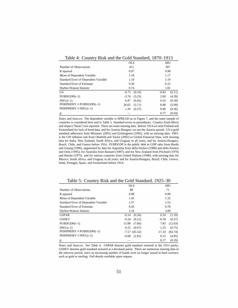
Table 4: Country Risk and the Gold Standard, 1870–1913OLS AR1

Number of Observations 411 397R squared 0.97 0.98Mean of Dependent Variable 1.18 1.17Standard Error of Dependent Variable 1.10 1.10Standard Error of Estimate 0.30 0.22Durbin-Watson Statistic 0.74 1.81GS -0.75 (0.10) -0.83 (0.11)PUBDGDP(t–1) -3.76 (3.23) 2.69 (4.28)INFL(t–1) 0.47 (0.45) 0.10 (0.28)PERIPHERY × PUBDGDP(t–1) 26.02 (3.71) 8.48 (5.09)PERIPHERY × INFL(t–1) 1.29 (0.57) 0.49 (0.36)ρ — 0.77 (0.04)

Notes and Sources: The dependent variable is SPREAD as in Figure 7, and the same sample ofcountries is considered here and in Table 5. Standard errors in parentheses. Country fixed effectsand slopes (“betas” ) not reported. There are some missing data. Before 1914 we omit Finland andSwitzerland for lack of bond data, and for Austria-Hungary we use the Austria spread. GS is goldstandard adherence from Meissner (2001) and Eichengreen (1992), with no missing data. INFLis the CPI inflation rate from Obstfeld and Taylor (2002) or Global Financial Data, with missingdata for India, New Zealand, South Africa, and Uruguay in all years; and for Austria-Hungary,Brazil, Chile, and Greece before 1914. PUBDGDP is the public debt to GDP ratio from Bordoand Jonung (1996), augmented by data for Argentina from della Paolera (1988) and della Paoleraand Ortiz (1995); for Australia from Barnard (1987); and for New Zealand from Prichard (1970)and Hawke (1975). and for various countries from United Nations (1948); with missing data forMexico, South Africa, and Uruguay in all years; and for Austria-Hungary, Brazil, Chile, Greece,India, Portugal, Spain, and Switzerland before 1914.

Table 5: Country Risk and the Gold Standard, 1925–30OLS AR1

Number of Observations 88 71R squared 0.98 0.99Mean of Dependent Variable 1.45 1.32Standard Error of Dependent Variable 1.57 1.53Standard Error of Estimate 0.45 0.78Durbin-Watson Statistic 2.16 3.00GSPAR -0.14 (0.36) 0.24 (1.10)GSDEV -0.24 (0.21) -0.18 (0.57)PUBDGDP(t–1) 15.98 (7.66) 7.83 (12.63)INFL(t–1) 0.22 (0.07) 1.23 (0.75)PERIPHERY × PUBDGDP(t–1) -7.57 (45.52) -17.10 (82.74)PERIPHERY × INFL(t–1) -0.68 (1.81) 0.15 (4.85)ρ — 0.17 (0.29)

Notes and Sources: See Table 4. GSPAR denotes gold standard restored at the 1913 parity;GSDEV denotes gold standard restored at a devalued parity. There are numerous missing data inthe interwar period, since an increasing number of bonds were no longer issued in hard currencysuch as gold or sterling. Full details available upon request.

51

It is important to note that this pattern does not hold for the interwar period.For that era, the market seems to have been more discerning in its scrutiny of allborrowers’ public debt and inflation data. In these samples we also find no strongevidence of reputational persistence, perhaps further evidence of the fragile credi-bility associated with the interwar gold standard where markets seemed to pay moreattention to current behavior; that is, an autoregressive correction seems unwar-ranted (though this might also reflect the short duration of the interwar panel data).Based on our OLS findings for 1925–30, an interwar increase in public debt, in anycountry, core or periphery, equivalent to 10 percent of GDP could raise spreadsby as much as 75 to 150 basis points. A 10 percentage point increase in inflationwould have raised spreads by just 2 basis points, a very small, but statistically sig-nificant effect.61 This finding may help us to understand why many policymakersin the 1920s and 1930s so feared the market response to unbalanced public bud-gets, notwithstanding the countercyclical case for fiscal expansion (James 2001).In this period, being on gold was not, in itself, enough to soothe markets.

To recapitulate: unlike Bordo, Edelstein, and Rockoff (1999), we find verydifferent behavior of bond spreads in relation to the gold standard over the interwarperiod 1925–30 as compared to the pre-1914 period. This may be ascribed mainlyto differences in concept (use of around secondary-market bond yields in Londonversus new issues in New York) and differences in macroeconomic control variables(government debt rather than deficit). Of these features in our empirical approach,the first, at least, seems necessary if we are to make comparisons on an equalfooting with Bordo and Rockoff (1996).

Before 1914, we find that the gold standard did indeed confer a “seal of ap-proval,” whereas macro fundamentals, measured by public debt and inflation, seemto have affected the spreads of peripheral more than core countries. We infer thatadherence to gold by core countries was pretty much sufficient to confer credibility,whereas markets took a broader and more skeptical view of peripheral countries.For the interwar period, a return to gold after devaluation seemed slightly morecredible, notwithstanding the arguments that led Britain and other countries to re-turn to gold at par; indeed, returning at par yielded small benefits at best, and a

into debt before they started feeling the pain.” The limited set of core countries generally had publicdebt levels at which, according to Flandreau et al., “markets did not inflict massive punishments.”This may explain why we find insignificant debt effects under the classical gold standard for thecore subsample of countries.

61This effect, if extrapolated, might not be so small under some hyperinflationary conditions, aspertained in the interwar period in various countries, but such data are omitted from our sample,and, besides, we do not expect the relationship to remain linear under such extreme conditions.

52

return after devaluation (as in the case of France) might have been more beneficial.Moreover, for core and periphery countries alike, high public debts and inflationwere punished, suggesting that policymakers’ room for maneuver in fiscal andmonetary policy was further curtailed.

Both our results on the drop in spreads associated with going on gold, andon markets’ differential response to public debt and inflation prewar and interwar,suggest that the interwar gold standard was indeed seen as a pale imitation, and wasconsidered far less credible than its pre-1914 predecessor. It remains to reconcilethese results with findings such as those of Hallwood, MacDonald, and Marsh(1996) that indicate a credible gold standard during the late 1920s, at least in theshort term. Perhaps the bond markets adopted a longer perspective under whichprotracted adherence to unchanging gold parities seemed less probable than short-term adherence.

These findings on bond markets serve to illuminate how different the interwarglobal capital market was from its antecedent, the classical gold-standard regimeof 1870–1914. An image used quite often to describe this regime change in theglobal economy is one of Humpty Dumpty falling to pieces, and these preliminarystatistical results show cross-regime evidence on how those pieces were scattered.The findings offer persuasive evidence that the global convergence of the bondmarket prior to 1914, so clearly seen in the figure, had been replaced by some quitedifferent disintegrative forces after 1914.

3.2 The Upturn

After the immediate post-World War Two dislocations, the world economy beganto reconstitute its severed linkages, a process both promoting and promoted by thereturn of some degree of durable prosperity and peace. Postwar policy makers,through the IMF, successive multilateral trade liberalization rounds, current ac-count currency convertibility, and other measures, successfully promoted growingworld trade. By the late 1960s, the very success of these initiatives in forging trad-ing linkages among countries simultaneously made capital flows across bordersever more difficult to contain. As a result, the trilemma re-emerged with full force,and on a global scale, in the early 1970s. The Bretton Woods system, initiallydesigned for a world of tightly controlled capital movements, blew apart. Themajor industrial countries retreated to floating exchange rates.

While initially viewed as a temporary expedient, floating rates have remaineda durable feature of the international financial landscape. Floating rates helpedreconcile the social demand for domestic macroeconomic stabilization with the

53

interest of the business community for open markets in goods and assets. Someepisodes of exchange rate misalignment have prompted calls for renewed protectionand even capital-account restrictions. Some of these calls have been accommo-dated, but usually not in the form of across-the-board restrictions on internationaltransactions.

Other forces have also helped to promote liberalization. In Europe, the po-litical and economic rationales for a large single market have prompted ongoingfinancial liberalization; at the same time, the political (and, some argue, economic)imperative of stable exchange rates has pushed toward the logical conclusion of asingle currency, the euro. Other regions, likewise, have opted for fixed exchangerates, either by some form of ultra-hard peg or outright dollarization, in either casebending to the trilemma by giving up monetary policy autonomy.

Since the late 1980s, the drive toward capital-account liberalization in the de-veloping world is probably the most striking pattern in the evolution of globalcapital markets. Clearly one element has been the widespread failure in the pe-riphery of populist policies adopted in the 1980s and earlier. On a larger scale, thecollapse of the Soviet empire in the late 1980s also highlighted the advantages ofthe capitalist model. The resulting decline in Cold War tensions certainly held outthe promise of greater fluidity in private international capital. Whether exchangerates float or are fixed, there is much greater openness to private financial flowson the periphery than in the 1980s. In part a reflection of U.S. business inter-ests, American administrations have pushed developing economies to liberalize oncapital account; in some cases, liberalization ran far ahead of domestic financialsystems’ absorptive capacities, and clashed with national exchange rate policies.The resulting contradictions helped spark the developing country currency crisesof the latter 1990s. To attract productive capital from the industrial world remainsa prime goal on the periphery, however, and that requires market-oriented reforms,stable macro policies, and transparency in governance and legal systems.

There is, however, one critical dimension in which pre-1914 international cap-ital flows differ sharply in nature from what we see today, with important im-plications for the periphery: to see this we return to the distinction between netand gross international asset stocks. A cursory glance at the data reveals that thisproblem is very serious in recent decades, but relatively unimportant in the pre-1914 era of globalization. The reason is simple: in the late nineteenth century theprincipal flows were long-term investment capital, and virtually unidirectional atthat. There was one notable exception, the United States, where both inflows andoutflows were large. But in most cases key creditor nations, principally Britain,but also France and Germany, engaged in the financing of other countries’ capital

54

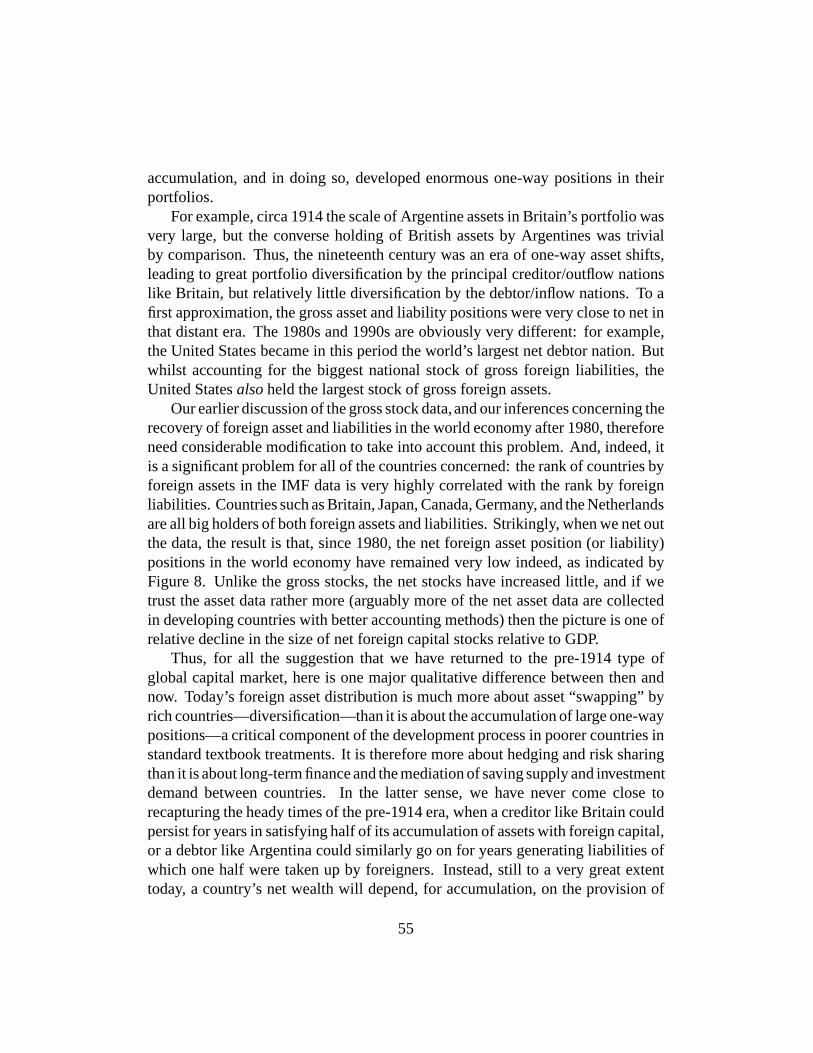
accumulation, and in doing so, developed enormous one-way positions in theirportfolios.

For example, circa 1914 the scale of Argentine assets in Britain’s portfolio wasvery large, but the converse holding of British assets by Argentines was trivialby comparison. Thus, the nineteenth century was an era of one-way asset shifts,leading to great portfolio diversification by the principal creditor/outflow nationslike Britain, but relatively little diversification by the debtor/inflow nations. To afirst approximation, the gross asset and liability positions were very close to net inthat distant era. The 1980s and 1990s are obviously very different: for example,the United States became in this period the world’s largest net debtor nation. Butwhilst accounting for the biggest national stock of gross foreign liabilities, theUnited States also held the largest stock of gross foreign assets.

Our earlier discussion of the gross stock data, and our inferences concerning therecovery of foreign asset and liabilities in the world economy after 1980, thereforeneed considerable modification to take into account this problem. And, indeed, itis a significant problem for all of the countries concerned: the rank of countries byforeign assets in the IMF data is very highly correlated with the rank by foreignliabilities. Countries such as Britain, Japan, Canada, Germany, and the Netherlandsare all big holders of both foreign assets and liabilities. Strikingly, when we net outthe data, the result is that, since 1980, the net foreign asset position (or liability)positions in the world economy have remained very low indeed, as indicated byFigure 8. Unlike the gross stocks, the net stocks have increased little, and if wetrust the asset data rather more (arguably more of the net asset data are collectedin developing countries with better accounting methods) then the picture is one ofrelative decline in the size of net foreign capital stocks relative to GDP.

Thus, for all the suggestion that we have returned to the pre-1914 type ofglobal capital market, here is one major qualitative difference between then andnow. Today’s foreign asset distribution is much more about asset “swapping” byrich countries—diversification—than it is about the accumulation of large one-waypositions—a critical component of the development process in poorer countries instandard textbook treatments. It is therefore more about hedging and risk sharingthan it is about long-term finance and the mediation of saving supply and investmentdemand between countries. In the latter sense, we have never come close torecapturing the heady times of the pre-1914 era, when a creditor like Britain couldpersist for years in satisfying half of its accumulation of assets with foreign capital,or a debtor like Argentina could similarly go on for years generating liabilities ofwhich one half were taken up by foreigners. Instead, still to a very great extenttoday, a country’s net wealth will depend, for accumulation, on the provision of

55

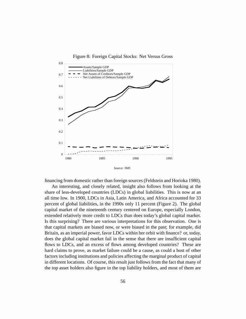
Figure 8: Foreign Capital Stocks: Net Versus Gross

0

0.1

0.2

0.3

0.4

0.5

0.6

0.7

0.8

1980 1985 1990 1995

Assets/Sample GDPLiabilities/Sample GDPNet Assets of Creditors/Sample GDPNet Liabilities of Debtors/Sample GDP

Source: IMF.

financing from domestic rather than foreign sources (Feldstein and Horioka 1980).An interesting, and closely related, insight also follows from looking at the

share of less-developed countries (LDCs) in global liabilities. This is now at anall time low. In 1900, LDCs in Asia, Latin America, and Africa accounted for 33percent of global liabilities, in the 1990s only 11 percent (Figure 2). The globalcapital market of the nineteenth century centered on Europe, especially London,extended relatively more credit to LDCs than does today’s global capital market.Is this surprising? There are various interpretations for this observation. One isthat capital markets are biased now, or were biased in the past; for example, didBritain, as an imperial power, favor LDCs within her orbit with finance? or, today,does the global capital market fail in the sense that there are insufficient capitalflows to LDCs, and an excess of flows among developed countries? These arehard claims to prove, as market failure could be a cause, as could a host of otherfactors including institutions and policies affecting the marginal product of capitalin different locations. Of course, this result just follows from the fact that many ofthe top asset holders also figure in the top liability holders, and most of them are

56

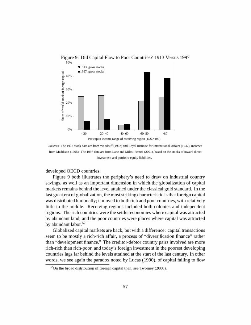
Figure 9: Did Capital Flow to Poor Countries? 1913 Versus 1997

0%

10%

20%

30%

40%

50%

<20 20–40 40–60 60–80 >80

Per capita income range of receiving region (U.S.=100)

Shar

e of

wor

ld s

tock

of

fore

ign

capi

tal

1913, gross stocks1997, gross stocks

Sources: The 1913 stock data are from Woodruff (1967) and Royal Institute for International Affairs (1937), incomes

from Maddison (1995). The 1997 data are from Lane and Milesi-Ferreti (2001), based on the stocks of inward direct

investment and portfolio equity liabilities.

developed OECD countries.Figure 9 both illustrates the periphery’s need to draw on industrial country

savings, as well as an important dimension in which the globalization of capitalmarkets remains behind the level attained under the classical gold standard. In thelast great era of globalization, the most striking characteristic is that foreign capitalwas distributed bimodally; it moved to both rich and poor countries, with relativelylittle in the middle. Receiving regions included both colonies and independentregions. The rich countries were the settler economies where capital was attractedby abundant land, and the poor countries were places where capital was attractedby abundant labor.62

Globalized capital markets are back, but with a difference: capital transactionsseem to be mostly a rich-rich affair, a process of “diversification finance” ratherthan “development finance.” The creditor-debtor country pairs involved are morerich-rich than rich-poor, and today’s foreign investment in the poorest developingcountries lags far behind the levels attained at the start of the last century. In otherwords, we see again the paradox noted by Lucas (1990), of capital failing to flow

62On the broad distribution of foreign capital then, see Twomey (2000).

57

to capital-poor countries, places where we would presume the marginal product ofcapital to be very high. And the figure may understate the failure in some ways:a century ago world income and productivity levels were far less divergent thanthey are today, so it is all the more remarkable that so much capital was directedto countries at or below the 20 percent and 40 percent income levels (relative tothe U.S.). Today, a much larger fraction of the world’s output and population islocated in such low productivity regions, but a much smaller share of global foreigninvestment reaches them.63

As we have noted, capital is discouraged from entering poorer countries by ahost of factors, and some of these were less relevant a century ago. Capital controlspersist in many regions. The risks of investment may be perceived differentlyafter a century of exchange risks, expropriations, and defaults. Domestic policiesthat distort prices, especially of investment goods, may result in returns too low toattract any capital. These conditions make a difficult situation much worse. Poorercountries must draw on foreign capital to a greater extent than they do at present ifthey are to achieve an acceptable growth in living standards. That is a fundamentalreason why reform and liberalization in the developing world, despite the setbacksof the late 1990s, are likely to continue, albeit hopefully with due regard to thepainful lessons learned in the recent past.

63See Clemens and Williamson (2001) for a detailed analysis of the determinants of Britishcapital export before 1914.

58

References

Barnard, A. 1987. Government Finance. In Australians: Historical Statistics, edited byW. Vamplew. Broadway, New South Wales: Fairfax, Syme & Weldon.

Baxter, M., and A. C. Stockman. 1989. Business Cycles and the Exchange-Rate Regime:Some International Evidence. Journal of Monetary Economics 23 (May): 377–400.

Bernanke, B. S., and K. Carey. 1996. Nominal Wage Stickiness and Aggregate Supply inthe Great Depression. Quarterly Journal of Economics 111 (August): 853–83.

Bhagwati, J. N. 1998. The Capital Myth. Foreign Affairs 77 (May–June): 7–12.Bordo, M. D., M. Edelstein, and H. Rockoff. 1999. Was Adherence to the Gold Standard a

“Good Housekeeping Seal of Approval” During the Interwar Period? National Bureauof Economic Research no. 7186, Working Paper Series (June).

Bordo, M. D., and B. Eichengreen, eds. 1993. A Retrospective on the Bretton WoodsSystem: Lessons for International Monetary Reform. Chicago: University of ChicagoPress.

Bordo, M.D., B. Eichengreen, and J. Kim. 1999. Was There Really an Earlier Period ofInternational Financial Integration Comparable to Today? In The Implications of theGlobalization of World Financial Markets, edited by A. H. Meltzer. Seoul: Bank ofKorea.

Bordo, M. D., and L. Jonung. 1996. Monetary Regimes, Inflation, and Monetary Reform:An Essay in Honor of Axel Leijonhufvud. In Inflation, Institutions, and Information:Essays in Honor of Axel Leijonhufvud, edited by D. F. Vaz and K. Vellupillai. London:Macmillan.

Bordo, M. D., and F. E. Kydland. 1995. The Gold Standard as a Rule: An Essay inExploration. Explorations in Economic History 32: 423–64.

Bordo, M. D., and H. Rockoff. 1996. The Gold Standard as a “Good Housekeeping Sealof Approval.” Journal of Economic History 56 (June): 389–428.

Bordo, M. D., and A. J. Schwartz, ed. 1984. A Retrospective on the Classical GoldStandard, 1821–1931. Chicago: University of Chicago Press.

Brezis, E. S. 1995. Foreign Capital Flows in the Century of Britain’s Industrial Revolution:New Estimates, Controlled Conjectures. Economic History Review 48 (February): 46–67.

Calomiris, C. W., and R. G. Hubbard. 1996. International Adjustment under the ClassicalGold Standard: Evidence for the United States and Britain, 1879–1914. In ModernPerspectives on the Gold Standard, edited by T. Bayoumi, B. Eichengreen, and M. P.Taylor. Cambridge: Cambridge University Press.

Cameron, R. E. 1993. A Concise Economic History of the World: From Paleolithic Timesto the Present. New York, Oxford University Press.

Campa, J. M. 1990. Exchange Rates and Economic Recovery in the 1930s: An Extensionto Latin America. Journal of Economic History 50 (September):677–82.

59

Chortareas, G. E., and R. L. Driver. 2001. PPP and the Real Exchange Rate-Real InterestRate Differential Puzzle Revisited: Evidence from Non-Stationary Panel Data. Bankof England. Photocopy (June).

Clemens, M., and J. G. Williamson. 2000. Where Did British Foreign Capital Go?Fundamentals, Failures and the Lucas Paradox 1870–1913. Working Paper Series no.8028, National Bureau of Economic Research (December).

Clinton, K. J. 1988. Transactions Costs and Covered Interest Arbitrage: Theory andEvidence. Journal of Political Economy 96 (April): 358–70.

Davis, L. E. 1965. The Investment Market, 1870–1914: The Evolution of a NationalMarket. Journal of Economic History 25: 355–99.

Davis, L. E., and R. E. Gallman. 2001. Evolving Financial Markets and InternationalCapital Flows: Britain, the Americas, and Australia, 1865–1914. Japan-U.S. Cen-ter Sanwa Monographs on International Financial Markets Cambridge: CambridgeUniversity Press.

Davis, L. E., and J. R. T. Hughes. 1960. A Dollar-Sterling Exchange, 1803–1895. Eco-nomic History Review 13 (August): 52–78.

della Paolera, G. 1988. How the Argentine Economy Performed during the InternationalGold Standard: A Reexamination. Ph.D. dissertation, University of Chicago.

della Paolera, G., and J. Ortiz. 1995. Dinero, Intermediación Financiera y Nivel deActividad en 110 Años de Historia Económica Argentina. Documentos de Trabajo no.36, Universidad Torcuato Di Tella (December).

Dornbusch, R. 1998. Discussion. Economic Policy 26 (April): 149–52.Drazen, A., and P. R. Masson. 1994 . Credibility of Policies versus Credibility of Policy-

makers. Quarterly Journal of Economics 109 (August): 735–54.Eatwell, J. 1997. International Financial Liberalization: The Impact on World Devel-

opment. Discussion Paper Series 12. New York: United Nations Development Pro-gramme.

Edelstein, M. 1982. Overseas Investment in the Age of High Imperialism. New York:Columbia University Press.

Edison, H. J., and W. R. Melick. 1999. Alternative Approaches to Real Exchange Ratesand Real Interest Rates: Three Up and Three Down. International Journal of Financeand Economics 4: 93–111.

Edison, H. J., and B. D. Pauls. 1993. A Re-Assessment of the Relationship between RealExchange Rates and Real Interest Rates: 1974–1990. Journal of Monetary Economics31 (April): 165–87.

Eichengreen, B. J. 1992. Golden Fetters: The Gold Standard and The Great Depression,1919–1939. Oxford: Oxford University Press.

Eichengreen, B. J. 1996. Globalizing Capital: A History of the International MonetarySystem. Princeton, N.J.: Princeton University Press.

Eichengreen, B. J., and M. D. Bordo. 2001. The Rise and Fall of a Barbarous Relic: The

60

Role of Gold in the International Monetary System. In Money, Capital Mobility, andTrade: Essays in Honor of Robert A. Mundell, edited by R. Dornbusch, M. Obstfeldand G. Calvo. Cambridge, Mass.: MIT Press.

Eichengreen, B. J., and M. Flandreau. 1996. The Geography of the Gold Standard.In Currency Convertibility: The Gold Standard and Beyond, edited by J. Braga deMacedo, B. J. Eichengreen and J. Reis. London: Routledge.

Eichengreen, B. J., and J. Sachs. 1985. Exchange Rates and Economic Recovery in the1930s. Journal of Economic History 45 (December): 925–46.

Einzig, P. 1937. The Theory of Forward Exchange. London: Macmillan.Einzig, P. 1968. Leads and Lags: The Main Cause of Devaluation. London: Macmillan.Elliott, G. 1999. Efficient Tests for a Unit Root When the Initial Observation is Drawn

from Its Unconditional Distribution. International Economic Review 40 (August):767–83.

Elliott, G., T. J. Rothenberg, and J. H. Stock. 1996. Efficient Tests for an AutoregressiveUnit Root. Econometrica 64: 813–836.

Escher, F. 1918. Elements of Foreign Exchange, 8th edition. New York: The BankersPublishing Company.

Feldstein, M., and C. Horioka. 1980. Domestic Savings and International Capital Flows.Economic Journal 90 (June): 314–29.

Feinstein, C. K. 1990. Britain’s Overseas Investments in 1913. Economic History Review43 (2):288–96.

Feis, H. 1931. Europe, The World’s Banker, 1870–1914: An Account of European ForeignInvestment and the Connection of World Finance with Diplomacy Before the War. NewHaven, Conn.: Yale University Press.

Flandreau, M., J. Le Cacheux, and F. Zumer. 1998. Stability Without a Pact? Lessonsfrom the European Gold Standard, 1880–1914. Economic Policy 26 (April): 115–62.

Flandreau, M., and C. Rivière. 1999. La Grande “Retransformation”? L’ IntégrationFinancière Internationale et Contrôles de Capitaux, 1880–1996. Économie Interna-tionale 78: 11–58.

Forbes, K., and R. Rigobon. 2000. Contagion in Latin America: Definitions, Measure-ment, and Policy Implications. Working Paper Series no. 7885, National Bureau ofEconomic Research (September).

Frieden, J. A. 1997. “Monetary Populism in Nineteenth-Century America: An OpenEconomy Interpretation.” Journal of Economic History 57 (June): 367-95.

Fujii, E., and M. Chinn. 2000. Fin de Siècle Real Interest Parity. Working Paper Seriesno 7880, National Bureau of Economic Research (September).

Gallarotti, G. M. 1995. The Anatomy of an International Monetary Regime: The ClassicalGold Standard 1880–1914. New York: Oxford University Press.

Goldsmith, R. W. 1985. Comparative National Balance Sheets: A Study of Twenty Coun-tries, 1688–1978. Chicago: University of Chicago Press.

61

Gourinchas, P.-O., and H. Rey. 2001. Stocks and Monies. Princeton University.Hallwood, C. P., R. MacDonald, and I. W. Marsh. 1996. Credibility and Fundamentals:

Were the Classical and Interwar Gold Standards Well-Behaved Target Zones? InModern Perspectives on the Gold Standard, edited by T. Bayoumi, B. Eichengreen,and M. P. Taylor. Cambridge: Cambridge University Press.

Hamori, S., and A. Tokihisa. 1997. Testing for a Unit Root in the Presence of a VarianceShift. Economics Letters 57: 245–253.

Haupt, O. 1894. Arbitrages et Parités. 8th edition. Paris: Librairie Truchy.Hawke, G. R. 1975. Income Estimation from Monetary Data: Further Explorations.

Review of Income and Wealth 21: 301-307.International Monetary Fund. 2001. World Economic Outlook. Washington, D.C.: Inter-

national Monetary Fund (October).James, H. 2001. The End of Globalization: Lessons from the Great Depression. Cam-

bridge: Harvard University Press.Jorion, P., and W. N. Goetzmann. 1999. Global Stock Markets in the Twentieth Century.

Journal of Finance 54 (June): 953–80.Kindleberger, C. P. 1984. A Financial History of Western Europe. London: George Allen

& Unwin.Kindleberger, C. P. 1986. The World in Depression, 1929–1939. Revised edition. Berkeley

and Los Angeles: University of California Press.Klug, A., and G. W. Smith. 1999. Suez and Sterling, 1956. Explorations in Economic

History 36 (July): 181–203.Lane, P., and G.-M. Milesi-Ferretti. 2001. The External Wealth of Nations: Measures

of Foreign Assets and Liabilities for Industrial and Developing Countries. Journal ofInternational Economics 55 (December): 243–62.

Lewis, C. 1938. America’s Stake in International Investments. Washington, D.C.: Brook-ings Institution.

Lewis, K. K. 1999. Trying to Explain Home Bias in Equities and Consumption. Journalof Economic Literature 37 (June): 571-608.

Lucas, R. E., Jr. 1990. Why Doesn’ t Capital Flow from Rich to Poor Countries? AmericanEconomic Review 80 (May): 92–6.

MacDonald, R., and J. Nagayasu. 2000. The Long-Run Relationship Between RealExchange Rates and Real Interest Rate Differentials: A Panel Study. InternationalMonetary Fund Staff Papers 47, no. 1: 116–28.

Maddison, A. 1995. Monitoring the World Economy. Paris: OECD.Margraff, A. W. 1908. International Exchange: Its Terms, Parts, Operations and Scope.

3rd edition. Chicago: Privately printed.Meese, R. A., and K. Rogoff. 1988. Was It Real? The Exchange Rate-Interest Differential

Relation over the Modern Floating-Rate Period. Journal of Finance 43 (February):933–48.

62

Meissner, C. 2001. A New World Order: Explaining the Emergence of the Classical GoldStandard. U.C. Berkeley. Photocopy.

Neal, L. 1990. The Rise of Financial Capitalism: International Capital Markets in theAge of Reason. Cambridge: Cambridge University Press.

Neal, L. 2000. How It All Began: The Monetary and Financial Architecture of Europeduring the First Global Capital Markets, 1648–1815. Financial History Review 7(October 2000): 117–40.

O’Rourke, K. H., and J. G. Williamson. 1999. Globalization and History: The Evolutionof a Nineteenth-Century Atlantic Economy. Cambridge: MIT Press.

Obstfeld, M. 1995. International Capital Mobility in the 1990s. In Understanding In-terdependence: The Macroeconomics of the Open Economy, edited by P. B. Kenen.Princeton, N.J.: Princeton University Press.

Obstfeld, M. 1998. The Global Capital Market: Benefactor or Menace? Journal ofEconomic Perspectives 12 (Fall): 9–30.

Obstfeld, M., and K. Rogoff. 1995. The Mirage of Fixed Exchange Rates. Journal ofEconomic Perspectives 9 (Fall): 73–96.

Obstfeld, M., and K. Rogoff. 2000. The Six Major Puzzles in International Macroeco-nomics: Is There a Common Cause? In NBER Macroeconomics Annual 2000, editedby B. S. Bernanke and K. Rogoff.

Obstfeld, M., and A. M. Taylor. 1998. The Great Depression as a Watershed: InternationalCapital Mobility in the Long Run. In The Defining Moment: The Great Depressionand the American Economy in the Twentieth Century, edited by M. D. Bordo, C. D.Goldin and E. N. White. Chicago: University of Chicago Press.

Obstfeld, M., and A. M. Taylor. 2002. Global Capital Markets: Integration, Crisis, andGrowth. Japan-U.S. Center Sanwa Monographs on International Financial MarketsCambridge: Cambridge University Press. In progress.

Officer, L. H. 1996. Between the Dollar-Sterling Gold Points: Exchange Rates, Parity,and Market Behavior. Cambridge: Cambridge University Press.

Oppers, S. E. 1993. The Interest Rate Effect of Dutch Money in Eighteenth-CenturyBritain. Journal of Economic History 53 (March): 25–43.

Paish, G. 1914. Export of Capital and the Cost of Living. The Statist (Supplement)(February 14, 1914): i–viii.

Peel, D. A., and M. P. Taylor. 2002. Covered Interest Rate Arbitrage in the Inter-WarPeriod and the Keynes-Einzig Conjecture. Journal of Money, Credit, and Banking 34(February): 000–000.

Perkins, E.H. 1978. Foreign Interest Rates in American Financial Markets: A RevisedSeries of Dollar-Sterling Exchange Rates, 1835–1900. Journal of Economic History38 (June): 392–417.

Platt, D. C. M. 1986. Britain’s Investment Overseas on the Eve of the First World War:The Use and Abuse of Numbers. New York: St. Martin’s Press.

63

Polanyi, K. 1944. The Great Transformation. New York: Rinehart.Prichard, M. F. L. 1970. An Economic History of New Zealand to 1939. Auckland: Collins.Rippy, J. F. 1959. British Investments in Latin America, 1822–1949: A Case Study in the

Operations of Private Enterprise in Retarded Regions. Minneapolis: University ofMinnesota Press.

Rodrik, D. 2000. How Far Will International Economic Integration Go? Journal ofEconomic Perspectives 14 (Winter 2000): 177–86.

Romer, C. D. 1992. What Ended the Great Depression? Journal of Economic History 52(December): 757–84.

Royal Institute of International Affairs. 1937. The Problem of International Investment.London: Oxford University Press.

Sachs, J. D., and A. Warner. 1995. Economic Reform and the Process of Global Integration.Brookings Papers on Economic Activity 1: 1–118.

Spalding, W.F. 1915. Foreign Exchange and Foreign Bills in Theory and Practice. London:Sir Isaac Pitman and Sons.

Sylla, R. E. 1975. The American Capital Market, 1846–1914: A Study of the Effects ofPublic Policy on Economic Development. New York: Arno Press.

Sylla, R. E. 1998. U. S. Securities Markets and the Banking System, 1790–1840. FederalReserve Bank of St. Louis Review (May/June).

Temin, P. 1989. Lessons from the Great Depression. Cambridge, Mass.: MIT Press.Triffin, R. 1957. Europe and the Money Muddle: From Bilateralism to Near-Convertibility,

1947–1956. New Haven, Conn.: Yale University Press.Twomey, M. J. 2000. A Century of Foreign Investment in the Third World. London:

Routledge.United Nations. 1948. Public Debt 1914–1946. Lake Success, NY: United Nations

Publications.Williamson, J. G. 1995. The Evolution of Global Labor Markets since 1830: Background

Evidence and Hypotheses. Explorations in Economic History 32 (April): 141–96.Williamson, J. G. 1996. Globalization, Convergence, and History. Journal of Economic

History 56 (June): 277–306.Woodruff, W. 1967. Impact of Western Man: A Study of Europe’s Role in the World

Economy 1750–1960. New York: St. Martin’s Press.

64