Global weak solutions for the initial-boundary-value ...hera.ugr.es/doi/15014940.pdf · Global Weak Solutions for the Initial–Boundary-Value ... Global Weak Solutions for the Initial

Mathematical Methods in the Applied SciencesMath. Meth. Appl. Sci., 21, 907—938 (1998)MOS subject classification: 35 Q72, 85 A05, 85D10

Global Weak Solutions for the Initial–Boundary-ValueProblems to the Vlasov–Poisson–Fokker–PlanckSystem

Jose A. Carrillo

Departamento de Matematica Aplicada, Facultad de Ciencias, Universidad de Granada, 18071Granada, Spain

Communicated by H. Neunzert

This work is devoted to prove the existence of weak solutions of the kinetic Vlasov—Poisson—Fokker—Planck system in bounded domains for attractive or repulsive forces. Absorbing and reflection-type boundary conditions are considered for the kinetic equation and zero values for the potential on theboundary. The existence of weak solutions is proved for bounded and integrable initial and boundary datawith finite energy. The main difficulty of this problem is to obtain an existence theory for the linearequation. This fact is analysed using a variational technique and the theory of elliptic—parabolic equationsof second order. The proof of existence for the initial—boundary value problems is carried out followinga procedure of regularization and linearization of the problem. ( 1998 B. G. Teubner Stuttgart—JohnWiley & Sons, Ltd.

1. Introduction and main result

This paper is intended to study initial—boundary-value problems for theVlasov—Poisson—Fokker—Planck (VPFP) system. This system consists of two coupledequations: the Vlasov—Fokker—Planck (VFP) equation to determine the distributionof particles and the Poisson equation to establish the self-consistent potential actingon the system. Let ) be a C= bounded domain with boundary ). Let f*0 be theprobability density of particles at time t located at position x3) with velocity v3RN

and let E be the self-consistent force field. The VFP equation is given by

f

t#(v )+

x) f#div

v((E!bv) f )!p*

vf"0, (1.1)

on (0,¹ )])]RN, ¹'0 and where b*0 and p'0 are constants related to thecollision between particles '(t,x) is the internal potential of the system and o ( f )

*Correspondence to: Jose A. Carrillo, Departamento de Matematica Aplicada, Facultad de Ciencias,Universidad de Granada, 18071 Granada, Spain

CCC 0170—4214/98/100907—32$17.50 Received 24 July 1997( 1998 B. G. Teubner Stuttgart—John Wiley & Sons, Ltd.

denotes the macroscopic mass density, given by

o( f ) (t,x)"PRN

f (t,x, v) dv. (1.2)

The force field E is obtained by solving the Poisson equation

E (t,x)"!+x'(t,x), !*

x' (t,x)"ho( f ) (t,x) on (0,¹ )]). (1.3)

The parameter h values $1 in the electrostatic and gravitational cases, respectively.We assume that the boundary is at fixed potential, i.e. we consider Dirichlet boundaryconditions for '(t, x) onto the boundary of ),

'(t,x)"0 on ). (1.4)

Neumann-type boundary condition can be also considered under minor changes. Inorder to solve equation (1.1) we need an initial data f

0and a boundary condition for

this kinetic equation. We consider absorbing-type or reflection-type boundary condi-tions. In the first one we know the inflow of particles on the boundary. For instance, ifwe think of a semiconductor device, we fix the physical input on the system. In thesecond one, we assume that the inflow of particles on the boundary is a function of theoutflow. For instance, this boundary condition seems to be physically reasonablewhen we have a huge fixed potential acting on the boundary preventing that theparticles come away. Let us introduce some notation to write explicitly those kinds ofboundary conditions. Let us consider the sets !x

$"Mv3RN such that $(v ) n (x))'

0N, for any x3), and !$"M(x, v)3)]RN such that $(v ) n (x))'0N, where n(x) is

the outward unit normal onto the boundary of the domain ). Denote by c$

f and c fthe traces of f on &T

$"(0,¹ )]!

$and &T"(0,¹ )])]RN, respectively, when

these traces are meaningful (see section 2). The absorbing-type boundary condition iswritten as

f (t,x, v)"g (t,x, v) on &T~1

, (1.5)

where g is a positive function. Reflection-type boundary conditions for kinetic equa-tions are integral relations between the density of particles coming out of an infinitesi-mal section of the boundary at a given time and the density of the particles impingingupon the same boundary section. Precisely, given x3) and t'0 we will assume that

c~

f (t,x, v)"ar P!x

`

R(t,x; v, v*) c`

f (t,x, v*) dv*, (1.6)

for any v3!x~

, with 0)ar)1. The scattering kernel R represents the probability that

a particle with velocity v* at time t striking the boundary at x reemerges in the sameinstant with velocity v. Specular and reverse reflection are particular cases of theabove relation (see Reference 9).

Let us introduce the set ¸p(&T$

; D v ) n (x) DdS dvdt) of functions f such that D f Dp isintegrable in &T

$with respect to the standard kinetic measure Dv ) n(x) DdSdvdt, where

dS is the Lebesgue measure on ). In the sequel, we denote it by ¸p(&T$

). Let us definethe current density, the kinetic energy, the potential energy and the entropy of the

908 J. A. Carrillo

Math. Meth. Appl. Sci., 21, 907—938 (1998)( 1998 B. G. Teubner Stuttgart—John Wiley & Sons, Ltd.

system, respectively, as

j ( f ) (t,x)"PRN

v f (t,x, v) dv, K ( f ) (t)"P)]RN

Dv D2 f (t,x, v) d(x, v),

P ( f ) (t)"P)'(t,x) o( f ) (t,x) dx and S ( f ) (t)"P)]RN

f log f d(x, v).

Firstly, we focus our interest on the VPFP system with absorbing-type law: Equations(1.1) and (1.3) with boundary conditions (1.4) and (1.5) and initial condition f

0. From

now on, we denote this problem by (VPFP$

!). Also, we denote by (VPFP$

3) the

problem with reflection-type boundary conditions, i.e. (1.6) instead of (1.5). Here, wemean by $ the interaction type between the particles. Let us introduce the setQ

T"[0,¹[])1 ]RN. We aim for weak solutions (in distributional sense) of the

problem (VPFP$

!). Precisely, f3¸= (0,¹; ¸1()]RN )) for any ¹'0, is a weak

solution of the problem (VPFP$

!) if, for any ¹'0, DE D f is locally integrable on Q

T,

PQT

f Aut

#(v ) +x)u!b (v ) +

v)u#(E )+

v)u#p*

vuBd(t,x, v) (1.7)

#P)]RN

f0u (0, x, v) d (x, v)#P&T

~

Dv ) n(x) D g udS dv dt"0,

for any u3C=0

(QT) such that u"0 on &T

#, where E"!+

x' with '3¸=(0,¹ ;

¼1,p0

())), 1)p(R a weak solution of (1.3). The main result of this work is thefollowing.

Theorem 1.1. Assume that f0*0 belongs to ¸1W¸=()]RN ) such that

Dv DN f03¸1()]RN ) with finite potential energy and that g*0 belongs to ¸1W¸=(&T

!)

with finite kinetic energy, that is, D v D2g3¸1(&T!

) for any ¹'0. ¹hen, the problem(VPFP`

!) has a global weak solution f*0 satisfying the following properties:

(i) f3¸=(0,¹ ; ¸1W¸=()]RN)) for any ¹'0.(ii) o ( f )3¸= (0,¹ ; ¸p())) for any 1)p)(N#2)/N and any ¹'0.(iii) j( f )3¸=(0,¹ ; ¸p ())) for any 1)p)(N#2)/(N#1) and any ¹'0.(iv) '3¸=(0,¹ ; ¼1,p

0W¼2,p())) for any 1)p)(N#2)/N and any ¹'0. Fur-

thermore, ' is a weak solution of Poisson’s equation (1.3).(v) ¹he solution has finite total energy for any time t and N)4.

An analogous result will be proved for the (VPFP~!

) problem with N)3. The effectof an external potential on our system could be also assumed. The existence of globalweak solutions for the (VPFP`

3) problem can be shown with similar properties under

suitable assumptions on R and finite initial entropy. However, we cannot study the(VPFP~

3) problem using these arguments.

The VPFP system in x, v3RN has been extensively studied during the last years.Existence and uniqueness results have been obtained in several frameworks: classicalsolutions, weak solutions, renormalized solutions and functional solutions. We refer

Global Weak Solutions for the Initial—Boundary-Value Problems 909

( 1998 B. G. Teubner Stuttgart—John Wiley & Sons, Ltd. Math. Meth. Appl. Sci., 21, 907—938 (1998)

to References 5, 7, 8, 13, 23 and the references therein. Nevertheless, the VPFP systemon bounded domains has not been analysed so deeply. The basic difficulty of VPFPsystem on bounded demains is to prove the existence of the corresponding linearproblem. We will study this linear problem in the variational setting using a result dueto Lions [18]. A similar variational technique was used by Degond and Mas-Gallic[11]. However, this approach does not provide us with the necessary ¸1 and ¸=

bounds for the density f as well as estimates of the moments and entropy. In order toobtain these relations we use the theory of elliptic—parabolic equations introduced byFichera [14] and Oleinik [19, 20]. The regularity of the solutions was studied byKohn and Nirenberg [17]. In fact, the VFP equation is an elliptic—parabolic equationbut the results of regularity are not applicable in this case. Hence, to solve the linearVFP equation we approximate it by a sequence of linear elliptic—parabolic equationsdefined on a smoother sequence of domains for which the results of regularity in [17]can be applied.

The existence of weak solutions of initial—boundary value problems for kineticequations has been studied for the Boltzmann and for the Vlasov—Poisson systemwith absorbing-type or reflection-type laws (see References 1, 2, 10, 15, 16, 24). Thestudy of the asymptotic behaviour in bounded domains with reflection-type boundaryconditions has been carried out in Reference 4 for the VPFP system and in Reference12 for the Vlasov—Poisson—Boltzmann system. These works showed that the largetime asymptotic of the corresponding systems are described by maxwellians deter-mined by the initial data and the limit potential.

The paper is structured as follows: in section 2 we analyse the corresponding linearproblem using a variational technique. Section 3 is devoted to approximate the linearVFP equation by elliptic—parabolic equations to derive the ¸1 and ¸= estimates,estimates on the moments and on the entropy. Section 4 is intended to prove Theorem1.1. With this purpose, we have to regularize and linearize the problem (VPFP`

!). The

regularization preserves the control of the energy which is the basic tool in kineticequations theory to get a weak solution when we pass to the limit. Firstly, we provethe existence of a solution for the regularized problem via a linearization and theresults of section 3. Later, we obtain Theorem 1.1 using the boundedness of the kineticenergy. Section 5 is focused on the existence of global weak solutions for the problems(VPFP`

r) by means of an approximation using problems of type (VPFP`

!).

Sections 2 and 3 can be read independently of the rest of the paper. The existence ofsolution for the linear problem and its properties are relevant for sections 4 and 5.

2. The linear VFP equation I

The basic difficulty of analysis of the VPFP system in bounded domains is theexistence of solution for the linear VFP equation. The main disadvantage of this linearequation is the absence of a fundamental solution for the arising degenerate parabolicequation. Here, the ‘degenerate’ character must be understood in the sense that thematrix of the coefficients of second-order derivatives is positive semidefinite. Through-out the next two sections, we assume the presence of a known force field E

0which is

bounded at any time, i.e. E03¸=(0,¹ ; ¸=())) for any ¹'0. The VFP equation to

910 J. A. Carrillo


determine the distribution of particles in the ensemble ) is given by

f

t#(v )+

x) f#div

v((E

0!bv) f )!p*

vf"h, (2.1)

on (0,¹)])]RN. Hence, h is a positive source-term in ¸1W¸=(QT) for any ¹'0.

We are going to analyse equation (2.1) together with the initial conditionf03¸1W¸=()]RN) and f"g on &

~, g3¸1W¸=(&T

~) for any ¹'0. From now on,

we consider weak solutions of (2.1) in the standard distributional sense. In order tosolve this linear problem in a variational setting we are going to apply a theorem offunctional analysis due to Lions [18] which was used in Reference 11 to solve a 1-DFokker—Planck equation.

Theorem 2.1 (Lions [18]). ¸et H be a Hilbert space provided with the inner product( ) , ) ) and the norm DD ) DD. ¸et FLH be a subspace provided with a prehilbertian norm D ) D,such that the injection of F into H is continuous. ¸et us consider a bilinear forma :H]FPR, such that a ( ) , u) is continuous on H for any u3F and such thata(u,u)*a Du D2 for any u3F with a'0. ¹hen, given a linear form ¸3F@ continuouswith the norm D ) D, there exists a solution u3H of the problem: a(u, u)"¸(u) for anyu3F.

To apply the previous result to VFP problem, let us introduce the Hilbert spaceH"M f3¸2(Q

T), such that +

vf3¸2 (Q

T)N. Let us denote by Tb the transport oper-

ator, given by Tb f" f/ t#(v )+x) f!b (v ) +

v) f. We define the Hilbert space Y by

Y"M f3H, such that Tb f3H@N, where H@ is the dual of H. ( ) , ) )H{, H

stands for thedual relation between H and its dual. The norms in H and Y are defined by

DD f DD2H"DD f DD2

L2 (QT )#DD+

vf DD22 (Q

T) and DD f DD2Y"DD f DD2

H#DDTb f DD2

H{.

Theorem 2.2. ¸et h3¸2 (QT), f

03¸2()]RN) and g3¸2(&T

~), for any ¹'0. ¹hen,

there exists a weak solution of the »FP problem f3Y, for any ¹'0.

Proof. In order to apply Theorem 2.1, we consider the equation

fMt

#e~bt(v ) +x) fM#ebt(E

0 )+v) fM!pe2bt*

vfM#j fM"h1 , (2.2)

on (0,¹ )])]RN, where h1 "e!(j#Nb)t h (t,x, e~btv). This equation comes formally byderiving the equation for fM"e!(j#Nb)t f (t,x, e~btv), with any j*0. A weak solutionof equation (2.2) is a function fM3H such that

PQTA!fM

u

t!fM e~bt(v ) +

x)u#ebtu (E

0 )+v) fM Bd(t,x, v) (2.3)

#PQT

(pe2bt+vf )+

vu#j fM u ) d(t,x, v)"PQ

T

h1 u d(t,x, v)

#P)]RN

f0u (0, x, v) d(x, v)#P&T

~

e~bt Dv ) n(x) D gN u dSdv dt



for any u3C=0

(QT) with u"0 on &T

`. We first prove the existence of a solution in

H of equation (2.2) with initial condition f0

and boundary values gN "e!(j#Nb)t

g(t,x, e~btv) on &T~

. Later, we will define f by f"e(j#Nb)t fM (t,x, ebtv) and we will checkthat this is a solution of our original problem.

Let F be the set of functions u3C=0

(QT) with u"0 on &T

`. F is a subspace of

H with continuous injection and we define the prehilbertian norm

Du D2F"DDu DD2

H#1

2DDu DD22(&T

~; e~btDv ) n(x) DdSdvdt )#1

2DDu (0, ) ) DD22 ()]RN) .

It is obvious that the inclusion of F into H is continuous. We define the bilinear forma :H]FPR as the left-hand side of equation (2.3) and the continuous bounded linearoperator ¸ on F given by

¸ (u)"PQT

h1 u d(t,x, v)#P)]RN

f0u (0,x, v) d(x, v)

#P&T~

e~bt Dv ) n (x) DgN u dSdv dt.

To find a solution fM on H of equation (2.3) is equivalent to find a solution fM on H ofa( fM , u)"¸(u) for any u3F. Now, let us check that a satisfies the properties stated inTheorem 2.1. Since fM belongs to H and E

03¸=(0,¹ ;¸=())), it is easy to see that

a( ) ,u) is continuous in H. To verify the coercivity of a, let us note that the divergencetheorem implies that the integral of ebtu (E

0 )+v)u on Q

Tvanishes and

!PQTAu

u

t#ue~bt (v )+

x)uBd(t,x, v)

"

1

2 P)]RN

Du (0,x, v) D2 d(x, v)#1

2 P&T~

e~bt Dv ) n (x) D Du D2dSdvdt.

Therefore, we conclude that

a(u,u)"PQT

(pe2bt D+vu D2#ju2) d(t, x, v)

#

1

2 P)]RN

Du(0,x, v) D2d(x, v)#1

2 P&T~

e~bt Dv ) n(x) D Du D2 dSdv dt,

which can be bounded from below as a(u,u)*min(1, p, j) Du D2F. Thus, Theorem 2.1

implies the existence of fM on H satisfying (2.3). Now, we define f (t,x, v)"e(j#Nb)t fM (t,x, ebtv). It is straightforward to check that f3H, for any ¹'0. Given anyu on F we consider uJ "ejtu (t,x, e~btv). Since u8 belongs to F, equation (2.3) is validfor uJ . Making the change of variables v@"e~btv, it is easy to deduce that f3H verifies

PQTA!f

u

t!f (v ) +

x)u#u ((E

0!bv) )+

v) f#p+

vf ) +

vuBd(t,x, v)

"PQT

hud(t,x, v)#P)]RN

f0u(0, x, v) d(x, v)#P&T

~

Dv ) n (x) Dg udSdv dt

912 J. A. Carrillo


for any u3C=0

(QT) with u"0 on &T

`. Thus, f3H satisfies the following equation in

the sense of distributions in (0,¹ )])]RN

f

t#(v )+

x) f#div

v((E

0!bv) f )!p*

vf"h.

Moreover, since divv(E

0f )!p*

vf!Nb f is a linear bounded functional on H, the

transport term Tb f3H@. Hence, f3Y and equation (2.1) is verified in H@. K

Once we have proved the existence of a solution f3Y of VFP problem, we mustspecify in what sense the traces of f on &T

~are well-defined. A survey of classical trace

results in kinetic theory can be found in [9] when we have that the free transport termT

0f3¸p(Q

T) for some p. However, we cannot apply these results since we only know

Tb f3H@. To define the traces we use again the ideas in [11] that we sketch in thefollowing lemma. We will denote by Ttb the adjoint operator of Tb . Let us point outthat for f3H the properties Tb f3H@ and Ttb f3H@ are equivalent.

Lemma 2.3. f3Y has trace values on c$f3¸2 (&T$

) and f (t, ) )3¸2()]RN ) for any0)t)¹. Moreover, given f

1, f

23Y the following Green-type identity holds,

(Tb f1, f

2)H{,H

#(Ttb f2, f

1)H{,H

"P)]RN

[( f1

f2) (¹, x, v)!( f

1f2)(0, x, v)] d(x, v)#P&T

(v ) n(x)) c f1c f

2dSdv dt.

Proof. Let us consider YI the set of C=0

functions on [0,¹]])1 ]RN which vanish ona neighborhood of the points (0, x, v), (¹,x, v) for x3) and v3RN and of the points of[0,¹]])]RN such that v ) n (x)"0. Following the arguments in [3, 11] we havethat the set YI is dense on Y.

Let us take (3YI . Using a partition of unity we can assume, without of loss ofgenerality, that ( vanishes on three of the four parts in which we have divided theboundary of Q

T, namely, &T

~, &T

`, M(0,x, v)/x3), v3RNN and M(¹,x, v)/x3), v3RNN.

Assume that ( does not vanish on &T~

. By Green’s identity we have

PQT

((Tb(#(Ttb() d(t,x, v)"!P&T~

D v ) n (x) D (2dS dv dt.

Therefore, we have DD( DD22(&T~

))C DD( DDH

DDTb(DDH{

, and thus, DD( DD¸2(&T

~))C DD(DDY

for any (3YI . The rest of the lemma follows from straightforward arguments involv-ing the density of YI on Y. K

Let us show now that f the solution of the VFP equation (2.1) has g as trace valueon &T

~. Also, we study the uniqueness, positively and ¸2-estimate of f.

Proposition 2.4. f is equal to g on &T~

and verifies f (0,x, v)"f0(x, v). ¹here exists

a unique solution fQ3Y of the »FP problem. Moreover, this solution is positive and



f3¸=(0, ¹ ; ¸2 ()]RN)) for any ¹'0 with

DD f DD¸= (0,¹ ;¸2()]RN)))C(DD f

0DD¸2 ()]RN)#DDg DD

¸2(&T~

)#DDh DD¸2 (Q

T)) ,

where C depends on b and ¹.

Proof. Let us prove the first statement. Using the Green identity in Lemma 2.3 forf1"f and f

2"u for any u3C=

0(Q

T) with u"0 on &T

`we have

(Tb f , u)H{,H

#(T tbu, f )H{,H

"!P)]RN

( f u) (0,x, v) d(x, v)!P&T~

Dv ) n (x) D c!fu dSdv dt,

Taking into account that f3H is a solution of (2.1) in the sense of distributions and thedefinition of Tb f as element of H@, it is straightforward to deduce that

P)]RN

[( f0!f (0, ) ))u] (0, x, v) d(x, v)#P&T

~

Dv ) n(x) D [(g!c~

f )u] dS dvdt"0

for any u3C=0

(QT) with u"0 on &T

`.

Since the equation is linear, it is enough to prove that the unique solution of theVFP equation with zero initial data and zero data on &T

~is zero. Let f be a solution

of this problem on Y. Proceeding as in Theorem 2.2, we define the function fM asfM"e!(j#Nb)t f (t,x, e~btv), which verifies equation (2.2) with h"0. Moreover, weknow that fM has zero traces on &T

~and for t"0. Since f3Y, fM belongs to H and

T@b fM" fM /t#e~bt(v )+x) fM belongs to H. On the other hand, a similar result forT@b as

in Lemma 2.3 implies that Green’s identity is true. Thus, we apply the Green identityfor f

1"f

2"fM to obtain

2(T@b f @, fM )H{,H

"P)]RN

( fM 2 ) (¹,x, v) d(x, v)!P&T`

Dv ) n (x) D c`

fM 2dSdv dt.

Since fM satisfies equation (2.2) in H, we deduce that

(T@b fM , fM )H{,H

"PQT

(ebt fM (E0 )

+v) fM#pe2bt D+

vfM D2#j fM 2 ) d(t, x, v)"0. (2.4)

Since fM3H the divergence theorem implies that the integral of ebt fM (E0 )

+v) fM on

QT

vanishes. Therefore, we conclude that the integral of j fM 2 on QT

is negative and, asa consequence, fM and f are zero a.e. on Q

T.

The second part can be derived analogously by using Green’s identity with thenegative part of fM instead of fM proving that the negative part of fM is zero. To finish theproof, we use that

2(T@b f @, fM )H{,H

"P)]RN

[ fM 2(¹, ) )!f 20

] d(x, v)#P&T

e~bt (v ) n(x)) (c fM )2dS dvdt,

914 J. A. Carrillo


fM verifies equation (2.4) and similar arguments as in Theorem 2.2 to deduce that

DD fM (¹, ) ) DD22 ()]RN ))DD f0

DD22()]RN )#DDe~(b@2)@t gN DD22(&T~

)#2 PQT

fM hM d(t,x, v).

Applying Holder’s inequality, writing the values of fM , gN and hM and taking jP0 it isa simple matter to deduce the required estimate. K

The same arguments as in previous lemma allow us to prove that the weak solutionf3Y verifies for any (3C=

0(Q

T) and any ¹'0 that

PQT

f A(t

#(v )+x)(!b (v )+

v)(#(E

0 )+v)(#p*

v(Bd(t,x, v)

#P)]RN

f0( (0,x, v) d(x, v)"P&T

(v ) n (x)) c f (dS dvdt. (2.5)

3. The linear VFP equation II

Until now, we have proved the existence of a unique solution on Y satisfying theproperties of proposition 2.4. Nevertheless, if we want to study the behavior of thephysical relevant quantities: mass, moments and entropy, we cannot obtain themdirectly. Formally, these estimates could be derived multiplying the VFP equation bysuitable functions and then applying divergence theorem. Since the solution is notknown to be smooth, we cannot proceed in this way. With this aim, we are going toapproximate the VFP equation by a sequence of smoother problems than the VFPproblem. Passing to the limit and using a uniqueness argument we will prove that theprevious solution f will have similar properties to the relations 1—5 stated in Reference4 and then, the mass, energy and entropy identities are verified in classical sense.

We need to introduce some notation and to recall some results of the theory ofelliptic-parabolic equations of second-order. A linear elliptic—parabolic equation ofsecond-order is given by

¸u"aij (X)uij#bi (X)u

i#c (X)u"h, (3.1)

with A"(aij) a positive-semidefinite symmetric matrix, i.e., A(X )X@@ )X@ is non-

negative, for any X@3Rd and X3DM with DLRd a smooth domain (D3C= ). We haveused subscripts to denote differentiation and we have also used summation conven-tion.

The first difficulty to solve Dirichlet boundary problem for equation (3.1) is to settlethe necessary boundary conditions, i.e. in which part of the boundary we must knowthe values of u. This difficulty was overcome by Fichera [14] proving that theboundary can be classified in four sets:

&3"MX3D such that aij v

ivj'0N,


ivj"0 and (bi!aij

j) v

i'0N,


ivj"0 and (bi!aij

j) v

i(0N



and &0"MX3D such that aij v

ivj"0 and (bi!aij

j) v

i"0N, where v(X ) is the

outward unit normal on the boundary D.Fichera [14] proved the existence of a unique bounded weak solution of the

Dirichlet boundary value problem knowing u on the sets &3X&

2. Independently,

Oleinik [19, 20] improved uniqueness and existence results of weak solutions in ¸p

spaces for piecewise smooth domains D. Regularity of the solutions is a difficult andincomplete subject. From the earliest works of Oleinik there appeared simple exam-ples in which the solution could develop discontinuities (see Reference 19). Also,Oleinik [20] and later, Kohn and Nirenberg could prove regularity when &

2X&

3is

closed or equivalently, D"&2X&

3if D is connected.

In fact, we can consider the equation (2.1) on QT"(0, ¹)])]RN as an ellip-

tic—parabolic equation in (t, x, v) variables and, if we identify the sigma sets, we have&3"0, &

2"&T

~XMt"0N, &

1"&T

`XMt"¹N and &

0is the subset of (0,¹ )])]RN

where v ) n (x)"0. However, &2

is not closed. Therefore, we have no regularity resultfor the bounded solutions of the VFP equation whose existence is assured by Fichera’sresult. Nevertheless, we will modify equation (2.1) to apply the regularity results inReference 17. The main theorem in Reference 17 asserts the following:

Theorem 3.1. ¸et us consider the boundary value problem for the equation (3.1) ona bounded C= domain DLRd with zero values on &

2X&

3. Assume that

(i) &2X&

3is closed.

(ii) !c(X) is very large positive compared to the derivatives of the other coefficientsup to second order, and to the derivatives of order less than 3 of the aij coefficients,as well as, to A~1 defined in the next item.

(iii) ¸et x03&

2and let / be a function defined in a neighborhood of x

0which vanishes

identically on D, +/(x0)O0 and /'0 in D. ¸et us denote by

k1"(bi!aij

j)/

iand k

2"(bi!aij

j) (/

r/

sars)

i.

¹hen, for a fixed integer K greater than 1 we have

A(x0)"1#

Kk2(x

0)

2k1(x

0)2'0.

(iv) ¹here exists e0'0 depending only on d such that

J¸0a

k1

(x0))e

0

A(x0)

K

on &2, with a"/

r/sars and ¸

0"aij 2

xix

j.

ºnder the above assumptions, for any h3HK(D), there exists a unique solution u ofequation (3.1) vanishing on &

2X&

3with u3HK(D!M

2) and u3HK/2 (M

2) for K even,

u3H(K#1)/2 (M2) for K odd, where M

2is a small neighbourhood of &

2.

The above theorem is also valid for less angular and unbounded domains (seeReference 17, p. 802). The main result of this section is the following one.

916 J. A. Carrillo


Theorem 3.2. Assume that f0*0 belongs to ¸1W¸=()]RN ) such that

Dv D2 f03¸1()]RN) and also assume that g*0 belongs to ¸1W¸=(&T

~) with finite

kinetic energy, that is, D v D2g3¸1(&T~

) for any ¹'0. ¹hen, equation (2.1) has a uniquepositive solution f3Y satisfying the following properties:

(i) f3¸=(0,¹ ; ¸1W¸=()]RN)) for any ¹'0.(ii) Dv D2 f3¸= (0,¹ ; ¸1()]RN)) for any ¹'0.(iii) +

vf3¸2 (Q

T) and f has trace values c

`f on ¸2 (&

`).

(iv) c`

f 23¸=(0,¹ ; ¸1(! ; Dv ) n (x) D dSdv)).(v) f satisfies equation (2.1) in the sense of property (2.5).

The basic idea to prove Theorem 3.2 is to approximate the cylinder QT

bya sequence of smooth domains De in which we consider a regularization of the VFPoperator to verify the hypotheses of Theorem 3.1. Moreover, since we need a controlof the moments in v of the distribution and the coefficients of first order in the VFPoperator are not bounded, we cut off the velocity space in a regular way. Thus, weapproximate the domains De by a sequence of bounded smooth domains De

R. For

these problems we obtain a sequence of solutions f e and f eR.

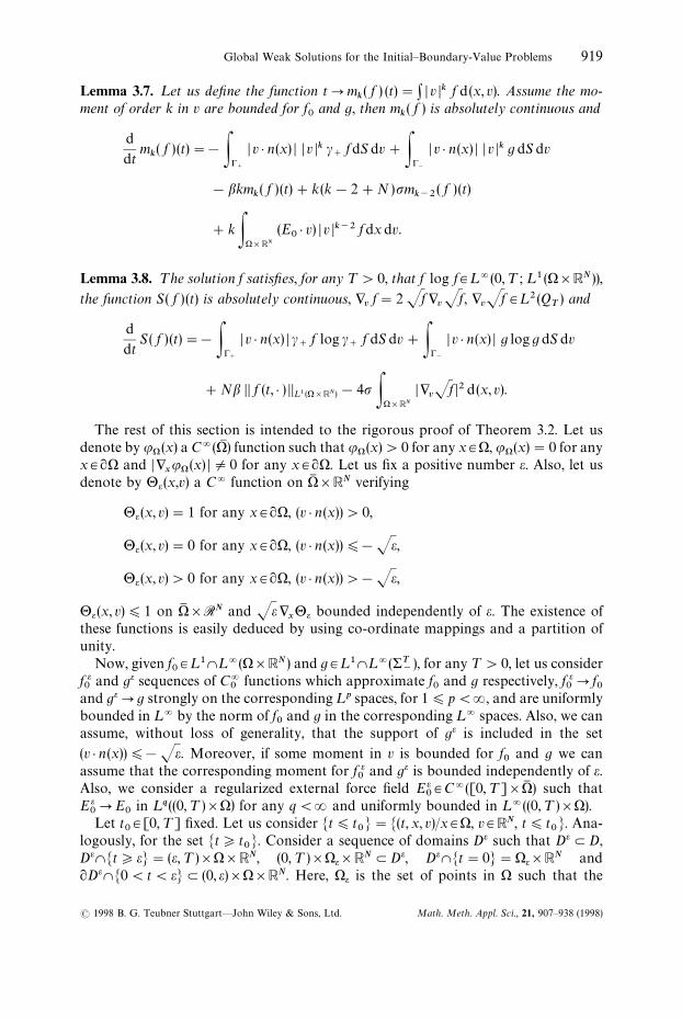
The previous result will be finished by taking the limit RPR and eP0 in theapproximate sequence of solutions. This procedure has been graphically summed upin Fig. 1 in which we draw the approximations of the domain in the 1-D case.

Before we proceed with the proof of this theorem let us point out that the propertiesof the solution f stated in Theorem 3.2 allow us to obtain ¸p a priori estimates, thecontinuity equation, the energy production identity and the entropy productionidentity. In the case of non-linear functions of f (entropy and ¸p estimates) we need touse a regularization of these functions. We refer to References 1, 4 and 6 for similararguments. In fact, section 3 in Reference 4 is devoted to prove that if we havea solution of the VPFP system satisfying the properties of the solution in Theorem 3.2,Dv D2c f3¸=(0,¹ ; ¸1(!

$)), ', '/t3¸=(0,¹ ; H1

0())), E3¸=(0,¹ ;¸= ())) and

Fig. 1. (a) The domain De in 1-D for any fixed velocity. (b) The domains cut off in velocity D eR

in 1-D fora fixed time



existence of traces of f (T0

f3¸2(QT); see References 4 and 9) then the continuity

equation, the energy production identity, the ¸p a priori estimates, and the entropyproduction identity are satisfied. In this case, the formal proof of these invariants iseasier since the regularity of E and ' is assured for the external field E

0. All the others

properties are satisfied except that D v D2c`

f3¸= (0,¹ ; ¸1(!`

)), which is straightfor-ward deduced in the arguments of the energy production identity, and the regularityof T

0f, which is easily substituted by the fact that Tb f3H@. Therefore, we can deduce

for the solution f of the linear VFP equation the following relations:

Lemma 3.3. ¹he solution f has trace values on ¸=(0,¹ ; ¸1(!`

)) and it verifies thecontinuity equation in integral form (balance of mass):

d

dtDD f (t, ) ) DD¸1 ()]RN)#P!

`

Dv ) n(x) D c`

f dv dS!P!~

Dv ) n (x) D gdv dS"0.

Lemma 3.4. ¹he solution f verifies the following equation:

d

dtDD f (t, ) ) DDpp ()]RN)#P!

`

Dv ) n (x) D (c`

f )pdv dS!P!~

Dv ) n (x) D gpdv dS

Nb(p!1) DD f (t, ) ) DDpp ()]RN)!pp (p!1) P)]RN

f (p~2) D+vf D2d(x, v),

for any 1)p(R. As a consequence, we have, for any 1)p)R, that

DD f DD¸= (0,¹ ;¸p ()]RN)))eNbT@p{ (DD f

0DD¸p ()]RN)#DDg DD

¸p(&T~

) ),

DD c`

f DD¸p(&T

`))eNbT@p{(DD f

0DD¸p()]RN )#DDg DD

¸p (&T~

) ).

Lemma 3.5. ¹he solution f satisfies the continuity equation on (0,¹)]) in the sense ofdistributions

d

dto ( f )#div

xj ( f )"0.

Lemma 3.6. ¹he function tP: Dv D2 f d(x, v) is absolutely continuous, Dv D2c`

f3¸=(0,¹ ;¸1 (!

`)) and the following identity is satisfied provided that E

0"!+

x'

0

d

dt AK ( f ) (t)#2P)'

0o ( f ) dxB

"!P!`

Dv ) n (x) D Dv D2c`

f dSdv

#P!~

Dv ) n (x) D Dv D2 g dSdv!2bK ( f ) (t)#2Np DD f (t, ) ) DD¸1 ()]RN) .

918 J. A. Carrillo


Lemma 3.7. ¸et us define the function tPmk( f ) (t)": Dv Dk f d(x, v). Assume the mo-

ment of order k in v are bounded for f0

and g, then mk( f ) is absolutely continuous and

d

dtm

k( f )(t)"!P!

`

Dv ) n(x) D Dv Dk c`

fdSdv#P!~

Dv ) n(x) D Dv Dk gdSdv

!bkmk( f )(t)#k (k!2#N )pm

k~2( f )(t)

#kP)]RN

(E0 )

v) Dv Dk~2 fdxdv.

Lemma 3.8. ¹he solution f satisfies, for any ¹'0, that f log f3¸=(0,¹ ; ¸1()]RN )),

the function S( f ) (t) is absolutely continuous, +vf"2 Jf +

vJf , +

vJf3¸2(Q

T) and

d

dtS ( f ) (t)"!P!

`

Dv ) n(x) D c`

f log c`

f dS dv#P!~

Dv ) n(x) D g log gdS dv

#Nb DD f (t, ) ) DD¸1 ()]RN)!4p P)]RN

D+vJf D2d(x, v).

The rest of this section is intended to the rigorous proof of Theorem 3.2. Let usdenote by u) (x) a C=()M ) function such that u) (x)'0 for any x3), u)(x)"0 for anyx3) and D +

xu) (x) DO0 for any x3). Let us fix a positive number e. Also, let us

denote by #e (x,v) a C= function on )1 ]RN verifying

#e (x, v)"1 for any x3), (v ) n (x))'0,

#e (x, v)"0 for any x3), (v ) n (x)))!Je,

#e (x, v)'0 for any x3), (v ) n (x))'!Je,

#e (x, v))1 on )1 ]RN and Je +x#e bounded independently of e. The existence of

these functions is easily deduced by using co-ordinate mappings and a partition ofunity.

Now, given f03¸1W¸=()]RN) and g3¸1W¸=(&T

~), for any ¹'0, let us consider

f e0

and ge sequences of C=0

functions which approximate f0

and g respectively, f e0Pf

0and gePg strongly on the corresponding ¸p spaces, for 1)p(R, and are uniformlybounded in ¸= by the norm of f

0and g in the corresponding ¸= spaces. Also, we can

assume, without loss of generality, that the support of ge is included in the set

(v ) n (x)))!Je. Moreover, if some moment in v is bounded for f0

and g we canassume that the corresponding moment for f e

0and ge is bounded independently of e.

Also, we consider a regularized external force field E e03C=([0,¹]])1 ) such that

E e0PE

0in ¸q((0,¹)])) for any q(R and uniformly bounded in ¸= ((0,¹)])).

Let t03[0,¹] fixed. Let us consider Mt)t

0N"M(t, x, v)/x3), v3RN, t)t

0N. Ana-

logously, for the set Mt*t0N. Consider a sequence of domains De such that DeLD,

DeWMt*eN"(e,¹)])]RN, (0,¹)])e]RNLDe, DeWMt"0N")e]RN andDeWM0(t(eNL(0, e)])]RN. Here, )e is the set of points in ) such that the



distance to ) is greater than e. We assume, without loss of generality, that ge andf e0

have their support in (e,¹ )])]RN and )e]RN, respectively. It is clear that wecan take a C= domain De except for Mt"¹N. We define the VFPe operator as

VFPe(u)"edivx[(u2) (x)##4e (x, v))+

xu]#p*

vu

!

u

t!(v ) +

x)u!((Ee

0!bv) )+

v)u!j (!ju), (3.2)

in De. Here, j is a positive number which can be considered as large as we need sincewe can change variables by defining uN "e~jtu(t,x, v). The domain De is a C=

piecewise domain. De has two smooth components: DeWMt(¹N and Mt"¹N. Theproperties of De imply that the outward unit normal is given by l"(0, n (x), 0) on(e,¹ )])]RN, l"(!1, 0, 0) on DeWMt"0N, l"(1, 0, 0) on Mt"¹N and l on theportion of the boundary DeWM0(t(eN that we can assume that has non-zero (x, v)component. The coefficients of the VFPe operator with the notation of (3.1) are givenby

A(t,x, v)"A0 0 0

0 e (u2)(x)##4e (x, v))IN

0

0 0 pINB ,

b(t,x, v)"(!1, e(2u)+xu)#4#3e +

x#e )!v,!E e

0#bv)

and c"!j, where IN

is the identity matrix of order N. Taking into account that thematrix A is positive definite in the normal direction for the points of the boundary

(e,¹ )])]RN where (v ) n (x))'!Je and that for (v ) n(x)))!Je we have(bi!aij

j)l

i"!(v ) n(x)), we can identify the sets &

ifor this operator finding &

0"0,

&1"Mt"¹N, &

2"M(t,x, v)3(e,¹ )])]RN with (v ) n (x)))!JeNXMt"0N and

&3"M(t,x, v)3(e,¹ )])]RN with (v ) n(x))'!JeNX(DeWM0(t(eN). We con-

sider the Dirichlet problem for the operator VFPe with boundary values e~jtgN e andfM e0

extensions by zero on &2X&

3of e~jtge and f e

0, respectively. Theorem 3.1 cannot be

applied since there is intersection between the closure of &1

and the closure of &2X&

3and we have non-zero values on &

2X&

3. Nevertheless, the other hypotheses of

Theorem 3.1 are easily satisfied. The second hypothesis is clear since we can take j aslarge as we need (note that we have to bound the derivatives of the coefficients b

inot

bi). The points of &

2verify the third and fourth hypotheses. Let us compute

a"/r/sars in this case. For the subject M(t,x, v)3(e,¹ )])]RN such that

(v ) n (x)))!JeN we can take the function u) as the function /, then we havea"e (u2) (x)##4e (x, v)) DD+

xu) DD2 and

(/r/sars )

i"e(2u)+

xu)#4#3e +

x#e) DD+x

u) DD2#e(u2)(x)##4e (x, v))

xi

DD+xu) DD2.

Therefore, (/r/sars)

i"0, k

2"0 and c"1 on this part of &

2. Computing ¸

0a we

deduce that ¸0a"e(u2)(x)##4e (x,v)) *

xa#p*

va. Thus, we have ¸

0a"4pe#3e *

v#e#

920 J. A. Carrillo


12pe#2e DD+v#e DD2"0 on this part of &

2. Therefore, the fourth hypothesis is also

satisfied. Now, we have to compute the same quantities for the subset Mt"0N. In thiscase, we can take as function / the function t. It is easy to see that a"a11"0 andthen k

2and ¸

0a vanishes. Hence, the third and fourth hypotheses of Theorem 3.1 are

satisfied.To avoid the difficulty of the non-empty intersection between the closures of &

2and

&1

we proceed as in [17] Theorem 3, Section 2.5. We consider a C= domain DI e suchthat DI eWMt(¹N"De and we define a new operator VF3 Pe extending VFPe to DI ebeing uniformly elliptic on DIM e!DM e. It is a simple matter to check that now, all theboundary belongs to &

2X&

3. Thus, we consider the Dirichlet problem for this new

operator with the same boundary values as before and zero in the new part of theboundary DI e!De which is included in &

3.

Finally, we have to deal with the boundary values. Theorem 3.1 is written withsecond member in the differential equation and zero boundary values. It is straightfor-ward to pass from one to the other in this case. In fact, since ) is infinitely smooth, wecan take an infinite differentiable function G on DIM e of compact support such thatG"e~jtg~e and G"fM e

0in the corresponding sets. Then, we can apply Theorem 3.1 to

the equation VFPe(u)"!VFPe (G) with zero values on the boundary. Moreover, wecan take the extension G such that

DDG DDHm (D)

)C(DDge DDHm (&T

~)#DD f e

0DDHm ()]RN )

), (3.3)

where C depends only on ¹.

Corollary 3.9. ¹he Dirichlet problem VFPe(u)"0 on De with u"gN e on(e,¹ )])]RN, u"fM e

0for Mt"0N extended by zero to the whole &

2X&

3, has a unique

classical solution f e. Moreover, f e3Hm(De ) for any m and f e3C= (De).

Remark 3.1. Using the stochastic differential equation theory (see Reference 21), anexplicit expression of the solution in terms of a Brownian motion can be deduced.Corollary 8.2 [21] or Theorem 3 [19] assure us the uniqueness of bounded solutionsof the Dirichlet problem for equation VFPe(u)"0. The maximum principle (Theorem1, Reference 19), the explicit expression of the solution and its uniqueness imply thefollowing consequences. The solution f e is positive and satisfies for any ¹'0 that

DD f e DD¸= (De))eNbT (DD f e

0DD¸=()]RN)#DDge DD

¸= (&T~

) ). (3.4)

The rest of this section is devoted to study the properties of the f e sequence ofsolutions and finally to show that the limit of f e when eP0 is the solution f of the VFPequation obtained in previous section. This fact allows us to derive importantproperties of f. To obtain ¸1 estimates and bounds on the moments we need to applydivergence theorem. Since the vector b is not bounded on D we cannot directly applydivergence theorem to these terms. Therefore, we will cut off the velocity space.

Let us consider a sequence of domains DeR3C= such that De

RW((0,¹)])]B

R~d)"DeW((0,¹)])]B

R~d) and DeRW((0,¹)])]B

R), where B

ris the euclidean ball cen-

tred at the origin with radius r and d'0 fixed and small enough. Assume R is largeenough to have the support in velocity of ge and f e

0included in De

R.



The same arguments as above can be applied for VFPe(u)"0 in the domain DeR

with boundary conditions: f"ge on DeRW((0,¹ )])]RN) and f"fM e

0for t"0

extended by zero to the set &2X&

3for this domain. Therefore, we obtain a unique

classical solution f eR

of VFPe(u)"0 in DeR

for these boundary conditions for anyR large enough. We will denote by fM e

Rthe extension by zero of these functions to

(0, T)])]RN. Let us study the properties of those solutions f eR. The same arguments

as in Remark 3.1 imply that the solution f eR

is positive and satisfies

DD fM eRDD¸= (0,¹ ;¸=()]RN)))eNbT(DD f e

0DD¸= ()]RN)#DD g e DD

¸=(&T~

) )

for any ¹'0. Since f eR3Hm(De

R) for any m, we can integrate VFPe(u)"0 on De

Rto

conclude using the divergence theorem that

P)]BR

fM eR(¹,x, v) d (x, v)!P)]B

R

f eRd(x, v)#P

T

0 P!~

ge (v ) n (x)) dS dvdt

!p PDeR

f eR

lv

dSR!e PDe

R

(u2)##4e ) f e

Rl

x

dSR"0, (3.5)

where we have used the boundary values of f eR. Here, l

xand l

vare the components in

x and v of the outward unit normal l of D eR

and dSR

the Lebesgue measure on this set.Due to the definition of the operator VFPe and the functions u) and #e we have

that the equation VFPe(u)"0 is uniformly parabolic locally in the points on DeR

where lxO0 except for the points (t,x, v)3De

Rwith x3) and (v ) n(x)))!Je .

However, in this portion of the boundary we have that (u2)##4e ) vanishes. Hence,Hopf’s maximum principle can be applied locally to these points of the boundary inwhich the operator is locally uniformly parabolic. Therefore, since f e

Ris positive and

takes the zero value on those portions of the boundary, we have that f eR

achieves itsminimum at all these points and then, the normal derivative at those points must benegative. Moreover, any outer derivative must be negative. The same reasoning can beapplied to those portions of the boundary of De

Rin which l

vO0. As a consequence,

f eR/l

x)0 on the points of De

Rwhere l

xO0 and (u2)##4e )O0 and f e

R/l

v)0 on

the points of DeR

where lvO0. Since (3.5) is valid for any ¹'0, we can easily infer

from equation (3.5) that

DD fM eRDD¸= (0,¹ ;¸1()]B

R)))DD f e

0DD¸1()]RN)#DD g e DD

¸1 (&T~

) .

The moments in v can be studied in a similar way. Multiplying VFPe(u)"0 for f eR

byDv Dk, integrating the resulting equation in De

Rand applying the divergence theorem we

can deduce that

P)]BR

Dv Dk fM eR(¹,x, v) d (x, v)!P)]B

R

Dv Dk fM e0d(x, v)

#PT

0 P!~

Dv Dk ge(v ) n (x)) dSdvdt#bk PD e

R

Dv Dk f eR

d(t,x, v)

922 J. A. Carrillo


!k (k!2#N ) pPDeR

Dv Dk~2 f eRd(t,x, v)!kPDe

R

(E e0 )

v) Dv Dk~2 f eR

d(t,x, v)

!p PDeR

Dv Dk f e

Rl

v

dSR!e PDe

R

Dv Dk (u2)##4e ) f e

Rl

x

dSR"0.

Proceeding as above, we conclude for any ¹'0 that

P)]BR

Dv Dk fM eR(¹, ) ) d (x, v))P)]B

R

D v Dk fM e0d(x, v)#k PDe

R

(Ee0 )

v) Dv Dk~2 f eRd(t,x, v)

#PT

0 P!~

Dv Dk ge Dv ) n (x) D dSdvdt

#k (k!2#N) p PD e

R

Dv Dk~2 f eR

d(t,x, v). (3.6)

We have the following classical interpolation result which give us a relationbetween the moments in v.

Lemma 3.10. ¸et jk(x) be the integral on RN of D v Dk f. Assume that f (x, v)3¸1()]RN)W

¸=()]RN), with f*0. If jk3¸1()), then j

k{3¸r()), 0)k@)k, with r"(N#k)/

(N#k@). Moreover,

DD jk{( f ) DD

¸r(RN ))C DD f DD (k!k@)/(N#k)¸= (R2N) DD Dv Dk f DD (N#k@)/(N#k)

¸1(R2N ) .

Using this lemma we can deduce the following result on the moments of thesequence of solutions fM e

R.

Lemma 3.11. All the moments in v of the distribution sequence fM eR

are bounded indepen-dently of R of any ¹'0.

Proof. In the sequel we denote by C several constants independent of R. We use theequation (3.6) for k"2. Then, we can estimate the last term of (3.6) by using Holder’sinequality

PDeR

(Ee0 )

v) f eR

d(t,x. v))DDEe0DD¸= (0,¹ ;¸N`2())) DD j ( fM e

R) DD

¸1(0,¹ ;¸ (N`2)@(N`1)())) .

Using Lemma 3.10 and estimate (3.4) we deduce that

PDeR

(Ee0 )

v) f eR

d(t,x. v))C PT

0AP)]B

R

Dv D2 fM eR

d(x, v)B(N`1)@(N`2)

dt.

Estimates (3.4), (3.7), (3.6) and the properties of ge and f e imply that

P)]BR

Dv D2 fM eR(¹,x, v) d (x, v))C#C P

T

0AP)]B

R

Dv D2 fM eR

d(x, v)B(N`1)@(N`2)

dt



for any ¹*0, C"C (¹ ). Therefore, the moment of order 2 of fM eR

is boundedindependently of R. We have proved that (1#Dv D2) fM e

R3¸=(0,¹ ; ¸1()]B

R)) with

a bound independent of R. In addition, we have for k*3 that

PDeR

(Ee0 )

v) Dv Dk~2 f eR

d(t,x. v))CPDeR

Dv Dk~1 f eR

d(t,x, v),

and finally, we conclude that

P)]BR

Dv Dk fM eR(¹,x, v) d (x, v))P)]B

R

Dv Dk fM e0(x, v) d (x, v)#DD Dv Dkge DD

¸1(&T` )

#k (k!2#N ) pPDeR

Dv Dk~2 f eRd(t,x, v)

#kC PT

0P)]B

R

Dv Dk~1 fM eR

d(t,x, v),

for any k*3 and any ¹*0. The announced result follows by induction on k. K

Now, we study the convergence of the sequence of solutions f eR

when R goes to R.Here, the set M()]RN) is the set of bounded measures.

Lemma 3.12. ¹he sequence fM eR

converges weakly-* in ¸=(0,¹ ; MW¸=()]RN)) to f e.As a consequence, if the moment of order k in v is bounded for g and f

0, then the moment

of order k for f e is bounded independently of e.

Proof. Previous estimates prove that fM eR

is bounded in ¸=(0,¹ ; ¸1W¸=()]RN )).Therefore, we can take a weak-* limit f * in ¸=(0,¹ ;MW¸=()]RN)). It is easy to seethat the limit function f * is a weak bounded solution of the equation VFPe (u)"0 onDe with boundary values ge and f e

0. Hence, by uniqueness of weak bounded solution

(see Reference 19 Theorem 3 for piecewise smooth domains) we have that f *"fM e .K

Finally, let us remark that Lemma 3.12 implies that

DD fM e DD¸= (0,¹ ;¸1 ()]RN)))DD f e

0DD¸1()]RN)#DD ge DD

¸1(&T~)

(3.7)

and the boundedness of the kinetic energy. Now, we can take the limit when eP0 toobtain the solution f.

Proof of ¹heorem 3.2. Using the bounds (3.4) and (3.7) together with the assumptionson the initial and boundary data, we have that the sequence fM e is bounded in ¸= (0, ¹ ;¸1W¸=()]RN)) independently of e, for any ¹'0. Also, we have that the kineticenergy Dv D2 fM e is bounded in ¸= (0,¹ ; ¸1()]RN)) independently of e, for any ¹'0.Therefore, there exists a limit f * such that

fM ePf * weakly | in ¸=(0,¹ ; MW¸=()]RN)),

Dv D2 fM ePF weakly | in ¸=(0,¹ ; M()]RN))

924 J. A. Carrillo


and

o( fM e)Po* weakly | in ¸= (0,¹ ; MW¸N@(N`2)())).

It is straightforward to see that F"D v D2 f *, f *3¸=(0,¹ ;¸1W¸=()]RN)) for any¹'0 and o*"o ( f * ). This fact can be seen in Reference 1.

On the other hand, since Ee0

converges to E0

in ¸q((0,¹ )])) for any q(R, it isa simple matter to pass to the limit in the weak formulation of the Dirichlet problemfor equation VFPe(u)"0 with test functions ("0 on &T

`and on the points (0, x, v)

with x3) to prove that f * is a weak solution of equation (2.1) with initial data f0and

boundary values g on &T~

, for any ¹'0. In order to prove that f * is the same as thesolution f obtained in Theorem 2.2, we proceed by showing that f *3Y and thus, usingthe uniqueness result in Y (Proposition 2.4). It is enough to prove that +

vf *3¸2(Q

T)

since, in this case, the operator divv(E

0f * )!p*

vf *!Nb f * is a linear bounded

operator on H and then, we have that the transport term Tb f * belongs to H@ andfinally, f *3Y. This argument was used in the proof of Theorem 2.2.

To show that +vf *3¸2(Q

T) we come back the sequence of f e

R. We can multiply

equation VFPe(u)"0 by f eR, integrate the resulting equation in De

Rand apply the

divergence theorem to conclude that

DD fM eR(¹, ) ) DD22()]B

R)!DD fM e

0DD22 ()]B

R)!P&T

~

D v ) n (x) D (ge)2dS dvdt

!NbDD f e DD22 (DeR)#2p !PDe

R

D+nf eRD2d(t,x, v)!2pPDe

R

f eR

lv

f eR

dSR

#2e PDeR

(u2)##4e ) D+xf eRD2d(t,x, v)!2e PDe

R

(u2)##4e ) f e

Rl

x

f eR

dSR"0,

where we have taken into account that divv(v f e

R) f e

R"div

v(v ( f e

R)2)#(N/2) ( f e

R)2.

Therefore, proceeding as above we have

PDeR

D+vf eRD2d(t,x, v))

1

2p(DDge DD22 (&T

~)#DD f e

0DD22()]RN) )#

Nb2p

DD f eRDD22(De

R) .

Thus, using estimates (3.4) and (3.7) we deduce that +vf eR

is bounded in ¸2(DeR)

independently of R and e. As a consequence, since the sequence fM eR

converges weakly-|in ¸=(0,¹ ; MW¸=()]RN)) to fM e we have that +

vf e is bounded in ¸2(De) indepen-

dently of e. Therefore, we can take a weak limit of the gradients +vfM e in ¸2(Q

T) to h*

and we easily infer that h*"+vf *. Therefore, +

vf *3¸2(Q

T). Finally, we do the

arguments referred above to conclude that f *"f the solution of the VFP equationgiven by Theorem 2.2. The properties of f are consequences of previous results. K

4. Regularization of the VPFP problem

The main difficulty of the VPFP problem is to obtain suitable estimates on thepotential E to apply a fixed point argument (see Reference 1) or to pass to the limit in



some regularization (see Reference 7). Since these estimates on the potentialE3¸=(0,¹ ; ¸= ()]RN)) are not available in the present form of the system, we mustmodify it by means of a regularization. For the VPFP system with )"RN, theregularization in Reference 7 was introduced to keep the energy estimates. The energycontrol is basic to obtain the limit. In a similar way for bounded domains, we need toregularize VPFP system and to keep the control of the energy. Some symmetry on theregularization is needed to control the energy. Then, we consider a modified VPFPesystem by substituting Poisson’s equation (1.3) by a greater order one;

!*'e (t,x)!e*2m`1'e(t, x)"ho ( f e ) (t,x) on (0,¹ )]), (4.1)

with m fixed large as necessary, e'0 and with Dirichlet boundary conditions

'e"*'e"2"*2m'e"0, (4.2)

on ). Here o ( f e ) is defined analogously to o ( f ) in (1.2). This type of regularizationwas used in Reference 1 and 2 for the Vlasov—Poisson system. The VPFPe systemconsists of the VFP equation to determine the distribution f e,

f et

#(v ) +x) f e#div

v((E e!bv) f e )!p*

vf e"0, (4.3)

on (0,¹)])]RN, coupled with the equation (4.1) to determine E e"!+x'e with

boundary conditions (4.2). The aim is to study the existence of weak solution of theVPFPe system with initial data f e

0and boundary values ge in the sense of (2.3), we

denote this problem by (VPFPea). f e

0and ge are sequences of C=

0functions which

approximates f0

and g respectively, f e0Pf

0and gePg strongly on the corresponding

¸p spaces, for 1)p(R, and are uniformly bounded by the norm of f0

and g in thecorresponding ¸= spaces. Taking into account the hypotheses on f

0and g in Theorem

1.1, we can assume, without loss of generality, that they verify

P&T~

Dv ) n (x) D Dv D2 Dge!g D dSdvdtP0, P)]RN

Dv DN D f e0!f

0DdxdvP0 (4.4)

and the sequences f e0

log f e0

and ge log ge are bounded in ¸1 ()]RN) and ¸1 (&T~

),respectively, independently of e'0. The last assumption on the sequence is in factconsequence of the following lemma [9] that we recall.

Lemma 4.1. Assume that f*0 verifies (1#Dv D2) f3¸1()]RN). ¹hen, f log~ f3¸1 ()]RN) and

P)]RN

f log~ f d(x, v))C(b,)) DD f DD¸1()]RN)#

1

2b P)]RN

Dv D2 f d(x, v) (4.5)

for any b'0. Also, if (1#Dv D2) f3¸1(&T ), then f log~ f3¸1 (&T) and a similar bound to(4.5) is satisfied.

Let us summarize the properties of the elliptic problem (4.1) and (4.2) (see Refer-ence 1).

926 J. A. Carrillo


Lemma 4.2. ¸et o3¸o()). ¹he problem !*'!e*2m`1'"ho on ), with Direchletboundary conditions '"*'"2"*2m'"0, on ) and m large enough, hasa unique solution in ¼4m`1,pW¼2m,p

0()) for 1)p(Rand verifies for any 1(p(R

that

DD' DD¼4m`2,p ())

)C(p, e) DD o DD¸p()) and DD' DD

¼2,p()))C(p) DD o DD¸p ()) .

Moreover, ' belongs to C2m`1()M ) and for any 1)q(N/(N!1) we have

DD' DD¼4m`1,q ())

)C(e) DD o DD¸1 ()) and DD' DD

¼01,q ()))C DD o DD

¸1()) .

To show the existence of solution for the modified problem, we construct aniterative scheme of linear problems approaching the (VPFPe

a) problem. Let us con-

sider oe0"o ( f e

0) and Ee

0"!+

x'e

0where 'e

0is the solution of problem (4.1)—(4.2) with

second member oe0. Now, we define f e

1as the solution of the VFP equation (2.1) with

E0"Ee

0, i.e.

f e1

t#(v ) +

x) f e

1#div

v((Ee

0!bv) f e

1)!p*

vf e1"0,

with f e1"f e

0for t"0 and f e

1"ge on &T

~, for any ¹'0. Next, we define Ee

1"!+

x'e

1where 'e

1is the solution of problem (4.1)—(4.2) with o"oe

1. By induction we define

f en

as the solution of

f en

t#(v ) +

x) f e

n#div

v((Ee

n~1!bv) f e

1)!p*

vf en"0, (4.6)

with initial condition f e0

and boundary values ge on &T~

, for any ¹'0. Here,Een"!+

x'e

nwhere 'e

nis the solution of problem (4.1)—(4.2) with o"oe

n. Theorem

3.2 and Lemma 4.2 prove that this sequence of functions is well-defined andf en3¸=(0,¹ ; ¸1W¸=()]RN))WY, Dv D2 f e

n3¸=(0,¹ ; ¸1()]RN)) and 'e

n3¸=(0,¹ ;

¼4m`1,qW¼1,q0

())WC2m ()1 )) for any ¹'0 and any 1)q)N/(N!1). Let us obtainestimates on the moments in velocity of the distribution sequence f e

n.

Lemma 4.3. All the moments in v of the distribution sequence f en

are bounded indepen-dently of n for any ¹'0, i.e. m

k( f e

n) (t))C(e, f e

0, ge, )).

Proof. Using the equation for the moments of order k (Lemma 3.7), we have that

d

dtm

k( f e

n) (t)"!P)]RN

(v ) n(x)) Dv Dk f en

dv dS!bkmk( f e

k) (t)

#k (k!2#N)pmk~2

( f en) (t)

#k P)]RN

(Een~1 )

v) Dv Dk~2 f en

dxdv (4.7)



Holder’s inequality, Lemmas 4.2 and 3.4 for p"1,Rand Sobolev’s inclusions implythat there exist two constants A and B depending upon ¹ and e but independent ofn such that

d

dtm

2( f e

n) (t))A#B m

2( f e

n) (t)(N#1)/(N#2) ,

for any 0)t)¹. The final arguments are exactly the same as in Lemma 3.11 using(4.7). K

Now, we obtain the regularity of the mass density by using the classical interpola-tion result, Lemma 3.10. As a consequence, the sequence f e

nsatisfies, for any ¹'0,

o( f en)3¸=(0,¹ ; ¸(N`k)@N())), D j ( f e

n) D3¸=(0,¹ ; ¸(N`k)@(N`1)())), (4.8)

for any k*1. Therefore, we have that o ( f en) and D j ( f e

n) D are bounded in ¸= ([0, ¹];

¸p())) independently of n, for any 1)p(R. Let us analyse the regularity of thepotential 'e

n. Lemma 4.2 assure us that the potential 'e

nbelongs to ¼4m`2,pW

¼2m,p0

()) and

DD'enDD¼4m`2,p ())

)C(p, e) DD o DD¸p()).

Continuity equation Lemma 3.5 implies that (/t)o( f en)#div

xj ( f e

n)"0. Now, we

can take the derivative with respect to t in Equation (4.1) to have

!*t

'en(t,x)!e*2m`1

t

'en(t,x)"!hdiv

xj ( f e

n)

together with Dirichlet boundary conditions. Again, classical interpolation resultsgive us that D j ( f e

n) D3¸=(0,¹ ;¸p ())) and thus, div

xj ( f e

n)3¼~1,p()), for any

1)p(R. As a consequence, classical elliptic theory implies that (/t)'e

n(t, x)3¸=(0,¹ ;¼4m`1,p ())), for any 1)p(R, with bounds independent of n.

The above regularity properties allow us to pass to the limit in n to obtain a solutionfor the modified VPFPe

aproblem.

Proposition 4.4. The modified problem VPFPeahas a positive solution f e which verifies

the following properties:

(i) f e belongs to ¸= (0,¹ ; ¸1W¸=()]RN )) for any ¹'0.(ii) Dv Dk f e3¸= (0,¹ ; ¸1()]RN)), for any ¹'0 and any k3N.(iii) o ( f e ) and D j ( f e) D are in ¸=(0,¹ ; ¸p ())), for any 1)p(R and ¹'0.(iv) 'e3L=(0,¹ ; ¼4m`1,pW¼2m,p

0()), for any 1)p(R and ¹'0.

(v) 'e/t3¸=(0,¹ ; ¼4m`1,p())), for any 1)p(Rand ¹'0.(vi) Ee3¸= (0,¹ ; ¼4m,p())), for any 1)p(Rand ¹'0.

Proof. We are going to use a result of compactness due to Aubin (see Reference 22,p. 271) which was used in Reference 1 for the VP system. Since 'e

n3¸=(0,¹ ;

928 J. A. Carrillo


¼4m`2,p())) and 'en/t3¸=(0,¹ ;¼4m`1,p())) independently of n, Aubin’s result

assure us that 'enis relatively compact in ¸q(0,¹ ;¼4m`1,p ())) for any 1)p, q(R.

Also, we can use the Ascoli—Arzela theorem to show that 'enis relatively compact in

¸=(0,¹ ;¼4m`1,p())) for any 1)p(R.Let us take a subsequence from 'e

n, that we denote with the same index, converging

to 'e. As a consequence, Een

converges to Ee"!+x'e in ¸=(0,¹ ;¸=())), for any

¹'0.Since o ( f e

n) is bounded in ¸= (0,¹ ;¸p ())) for any p(R, we can take a subsequence

which converges to o weakly | in ¸=(0,¹ ;¸p())) for any p(R and weakly in¸q(0,¹ ;¸p())) for any p, q(R.

On the other hand, we have that f en

is bounded in ¸= (0,¹ ;¸1W¸=()]RN))independently of n. Thus, we can find a subsequence which converges to f e weakly-|in ¸=(0,¹ ;MW¸=()]RN)) and weakly in ¸q (0,¹ ;¸p()]RN)) for any p, q(R.

Also, the sequence Dv Dk f en

converges weakly-| in ¸=(0,¹ ;M()]RN)) to somefunction Fk. Using the boundedness of the moments given in Lemma 4.3, it is easy toshow that o"o ( f e ) and Fk is given by the density D v Dk f e and then Dv Dk f e belongs to¸=(0,¹ ;¸1()]RN)). The proof of this fact can be seen in References 1 and 8.

Using the above properties, it is straightforward to pass to the limit in equation (1.7)for f e

nand to show that f e verifies equation (4.3) with initial condition f e

0and boundary

values ge. Also, 'e is the weak solution of equation (4.1) with the above regularity. Theregularity is derived from arguments above and Lemma 4.2. K

Now, we are going to study the properties of the solution f e. Firstly, we are going todeduce that f e belongs to Y.

Lemma 4.5. ¹he solution f e of the (VPFPea) problem belongs to Y. As a consequence, f e

has trace values on ¸2(&T ) and verifies the VFP equation in the sense of (2.5).

Proof. Firstly, let us prove that +vf e belongs to ¸2(Q

T). Since f e

nsatisfies Lemma 3.4

we have that

d

dtDD f e

n(t, ) ) DD22 ()]RN)#P!

`

Dv ) n(x) D (c`

f en)2dvdS!P!

~

D v ) n(x) D (ge)2dvdS

"Nb DD f en(t, ) ) DD22 ()]RN)!2pP)]RN

D+vf enD2d(x, v).

The estimates in Lemma 3.4 for p"2 imply that f en

is bounded in ¸2 ()]RN)independently of n. As a consequence, integrating previous relation we have that +

vf en

is bounded in ¸2 (QT) independently of n.

Since the sequence f en

is bounded in H independently of n, we can take a subsequ-ence converging to some limit weakly in H. It is easy to see that the convergence onthe weak topology of H implies the convergence on the weak topology of ¸2(Q

T).

Hence, the limit of the subsequence of f en

is f e3H. Also, we have that f e verifiesTb f e"!div

v(Ee f e)#p*

vf e#Nb f e, in the sense of distributions. Using that Ee is

¸=-bounded and that +vf e is bounded in ¸2(Q

T), we conclude that Tb f e is bounded

in H@. Therefore, f e3Y. The rest of the statements are included in section 2. K



Now, we can derive a priori estimates for the VPFPe problem. All the relationsobtained for the linear equation are valid since the properties in Reference 4 recalledin sections are verified for f e. Thus, Lemmas 3.3—3.8 are valid for f e substitutingE0

and '0

by E e and 'e.In order to prove the existence of solution of the VPFP system we need to get rid of

the e-regularization of the (VPFP!) problem by means of an energy control argument.

In fact, let us review the previous bounds to analyze their dependence on e.

Lemma 4.6. ¹he solution f e has the following properties.(i) ¹he sequence f e is bounded in ¸=(0,¹ ;¸p()]RN )) independent of e, for any

¹'0 and 1)p(R.(ii) In the electrostatic case, the total energy and the kinetic energy are bounded

independent of e'0, for any ¹'0 and any dimension N. If the gravitationalcase, for N)3 the same conclusion holds.

(iii) o ( f e ), j ( f e), 'e and 'e/t are bounded in ¸=(0,¹ ;¸ (N#2)/N ())), ¸=(0,¹ ;¸

(N#2)/(N#1) ())), ¸=(0,¹ ;¼2, (N#2)/N ())) and ¸=(0,¹ ;¼1, (N#2)/(N#1) ())), re-spectively, independent of e'0.

Proof. Using the ¸p bounds given in Lemma 3.4, we have that

DD f e DD¸= (0,¹ ;¸p()]RN )))eNbT@p{ (DD f e

0DD¸p()]RN)#DDge DD

¸p (&T~

) ),

for any 1)p)R. Then, taking into account the properties of the regularizedsequences f e

0and ge, the first statement is proved.

Since 'e(t, ) ) in ¼1,p0

()), for any p(R, is a weak solution of problem (4.1) we havethat

P)'eo ( f e ) dx"!hP)

'e*'edx!heP)'e*2m`1'edx

"hP)D+'e D2 dx#heP)

D*m+'e D2 dx.

Thus, using the energy production identity, Lemma 3.6, we get the following estimate:

E ( f e) (t))E ( f e) (0)#DD Dv D2ge DD¸1 (&T

~)#2Npt DD f e DD

¸= (0,¹;¸1()]RN)) , (4.9)

for any 0)t)¹ where E ( f ) is the total energy. In the electrostatic case the potentialenergy of the modified problems P ( f e )(t) is positive (h"1). Using the assumptions onthe moments of f e

0and ge (4.4), we have that K ( f e ) (0) and the norm of D v D2ge are

bounded independently of e. The last term is bounded independently of e due to thebalance of mass relation, Lemma 3.3. Finally, the initial potential energy is given by

P ( f e) (0)"P)'e(0,x)o ( f e

0) dx.

Holder’s inequality and Lemma 4.2 imply that P ( f e )(0))C DD o( f e0) DD2

LÈ ()). Using that

Dv DNf e0

is integrable, we can apply Lemma 3.10 to deduce that P ( f e ) (0) is bounded

930 J. A. Carrillo


independently of e. Therefore, since K ( f e ) (t) and P ( f e )(t) are positive, they arebounded independent of e. In the gravitational case the potential energy is negative.One can proceed using similar ideas as in References 1 and 7. In this way, Sobolevimbeddings imply that

DP ( f e ) (t) D)C DD f e DD¸=(0,¹ ;¸1 ()]RN)) DD'e DD

¸= (0,¹ ;¼2,(N`2)@N ())) .

Lemmas 4.2 and 3.10 assured that DP ( f e ) (t) D)C@ K( f e )(t)N@(N`2), with C@ indepen-dent of e. Therefore, using inequality (4.9) we deduce that the kinetic energy K ( f e) (t) isbounded independently of e.

The rest of the properties are direct consequences of the characteristics of the ellipticproblem, Lemma 4.2, and interpolation result, Lemma 3.10. K

Proof of ¹heorem 1.1. The bounds obtained in Lemma 4.6, Banach—Alaoglu theoremand Aubin’s result of compactness [22, p. 271] allow us to take a subsequence ofsolutions f e, that we denote with the same index, such that

f ePf weakly | in ¸= (0,¹ ;MW¸=()]RN)),

o( f e)Po weakly | in ¸=(0,¹ ;¸ (N#2)/N())),

j ( f e )Pj weakly | in ¸=(0,¹ ;¸ (N#2)/(N#1) ())),

Dv D2 f ePF weakly | in ¸= (0,¹ ;M ()]RN)),

'eP' weakly in ¸= (0,¹ ;¼2,(N`2)@2W¼1, (N`2)@N0

())),

'et

P

't

weakly in ¸=(0,¹ ;¼1, (N#2)/(N#1) ())),

EePE strongly in ¸=(0,¹ ;¸ (N#2)/(N#1) ()))

and

EePE weakly in ¸= (0,¹ ;¼1, (N#2)/(N#1)())).

Proceeding as in Proposition 4.4, it is easy to show that o, j and F are in fact o ( f ),j ( f ) and Dv D2 f , respectively. The above convergence results allow us to pass to thelimit in the weak formulation of (4.3) to obtain (1.7). By taking the limit in equa-tion (4.1) using the above regularity properties, it is a simple matter to prove that ' isa solution of Poisson equation (1.3). The rest of the properties are consequence of thecompactness of the corresponding sequences. Finally, let us remark that due toSobolev imbeddings, ¼1,(N`2)@N())P¸2 ()). K

Remark 4.1. We can obtain additional properties on the solution f. Using the ¸2-norm identity for the modified problems and similar arguments as in Lemma 4.5 weobtain that +

vf e is bounded independent of e in ¸2(Q

T). Thus, we have that f3H.



Remark 4.2. In the one- and two-dimensional case we have better properties on thesolutions. In fact, Sobolev imbeddings imply that the force field E3¸=(0,¹;¼1,=()))for N"1 and E3¸=(0,¹ ;¼1,p ())) for N"2 and any p(R. As a consequence, E isbounded and thus, the solution f3Y. The solution has traces on the boundary and allthe invariant equations are verified for the solution. For N)4 we can eliminate thehypothesis Dv DN f

03¸1()]RN) because of Sobolev imbeddings, ¼2,(N`2)@N())P¸s())

for any

1)s)s*"N2#2N

N2!2N!4and

N#2

2)s*.

5. Reflection-type boundary conditions

The reflection-type boundary law has been introduced for the Boltzmann equation[9, 16], for the Vlasov—Poisson system [2], for the Vlasov—Poisson—Boltzmann sys-tem [12] and for the VPFP system [4]. Given x3) and t'0 we will require that thephase space distribution function satisfies the boundary conditions:

c~

f (t,x, v)"arP!x

`

R(t,x; v, v*) c`

f (t,x, v* ) dv*,

for any v3!x~

, where R (scattering kernel) represents the probability that a moleculewith velocity v* at time t striking the boundary on x reemerges at the same instant andlocation with velocity v. Here, 0)a

r)1. Specular and ‘bounce-back’ reflections are

included in this setting for ar"1.

We will say that f is a weak solution of VFP equation with reflection-type boundaryconditions, (1.6), if

PQT

fAu

t#(v )+

x)u!b (v )+

v)u#(E ) +

v)u#p*

vuBd(t,x, v)

#P)]RN

f0u(0,x, v) d(x, v)"P&T

(v ) n (x))c fu dSdvdt, (5.1)

for any u3C=0

(QT), where c

$f satisfy (1.6). We can rewrite the boundary condition

(1.6) as c~

f"arR[c

`f ] in terms of an operator R defined by

(R[c`

f ]) (t, x, v)"P!x`

R(t, x; v, v*) c`

f (t, x, v*) dv*,

for any (t,x, v)3&T~

. We will assume that R has the following properties:

(i) R is non-negative.(ii) R verifies the following normalization:

Dv* ) n (x) D"P!x~

R(t,x; v, v*) D v ) n (x) Ddv. (5.2)

for any v*3!x`

.

932 J. A. Carrillo


(iii) ¸et us denote by M (v) the maxwellian at the wall (the maxwellian given by thetemperature of the thermal both surrounding the particles). R verifies

M(v)"P!x~

R(t,x; v, v*)M(v*) dv*. (5.3)

for any v3!x~

. In the case of the Boltzmann equation M(v) can depend on t and x.Nevertheless, for the VPFP system the maxwellian at the wall must be determinedby the temperature of the thermal both which s p/b, i.e.,

M(v)"A2npb B

~3@2expG!

b Dv D22p H .

(iv) R is a bounded linear operator from ¸p(&T`

) into ¸p(&T~

) with norm DDR DDpless than

unity, for any 1)p)R.

Lemma 5.1 (Cercignani et al. [9], Hamdache [16]). ¸et f be satisfying (1.6) with ar"1

and assume that (1#Dv D2#D log f D) f belongs to ¸1 (&T ). ¹hen, for any 0(t(¹, theflux of f vanishes through the boundary, that is,

P)]RN

(v ) n (x)) c fdSdv"0.

and the following relation between the flux of kinetic energy and the flux of entropythrough the boundary holds, that is,

P)]RN

(v ) n (x)) Ab2p

Dv D2#log c fB c f dSdv*0. (5.4)

From now on, we restrict the analysis to the electrostatic case. Firstly, we are going tostudy the case in which the distribution is not reflected completed (a

r(1). In this case,

we can approximate this problem by problems of absorbing-type boundary condi-tions and the traces functions have enough regularity to pass to the limit. The casear"1 is more complicated as we shall show later. In this case, there appears a loss of

regularity on the traces due to grazing collisions on the boundary near the velocityhyperplane (v ) n(x))"0 (see Reference 16, Remark 4.2).

To prove the existence of weak solution for the VPFP system with reflection-typeboundary conditions (1.6), with 0)a

3(1, instead of conditions (1.5), we proceed in

an analogous way as for the absorbing case. We carry out an e-regularization of thePoisson’s equation to control the energy and to get necessary estimates on the forcefield E. Also, we linearize not only the modified VPFPe corresponding problem butalso, the boundary conditions. Then, we approximate the problem (VPFP

3) by

a sequence of problems of type (VPFP!).

Assume that f03¸1W¸=()]RN) with Dv DN f

03¸1()]RN ) and has finite kinetic

energy, potential energy and entropy. Let us define the sequence f n by the solutions ofthe VFP equation

f n

t#(v )+

x) f n#div

v((En~1!bv) f n)!p*

vf n"0,



with initial condition f0

and boundary values given by c~

f n"a3R[c

`f n~1] on &T

~,

for any ¹'0 and n*2, c~

f 1"0. Here, En"!+x'n, where 'n is the solution of the

problem (4.1) and (4.2) with o"on and e"1/n. The existence and properties of thesequence f n are deduced with analogous arguments as in section three. Let us obtainthe basic properties which allow us to pass to the limit when nPR.

Lemma 5.2. ¹he sequence f n verifies

DDe~NbT@p{ c`

f n DDpp(&T`

))1

1!a3

DD f0DDpp()]RN)#anp

3DDe~NbT@p{ c

`f1DDpp(&T

`) , (5.5)

for any n, ¹'0 and 1)p)R. As a consequence, the sequence f n is boundedindependent of n in ¸=(0,¹ ;¸p ()]RN)) for any ¹'0 and 1)p)R.

Proof. Using similar estimates to those in Lemma 3.4, which are valid in this case, wehave that

DDe~NbT@p{ c`

f n DDpp(&T`

))DD f0DDpp()]RN)#DDe~NbT@p{ c

~f n DDpp(&T

`) .

The definition of the boundary values of f n and the properties of the operatorR implies that

DDe~NbT@p{ c~

f n DDpp(&T~

))aprDDe~NbT@p{ c

`f n~1 DDpp(&T

`) .

Thus, we find

DDe~NbT@p{ c`

f n DDpp(&T`

))DD f0DDpp()]RN)#ap

3DDe~NbT@p{ c

`f n~1 DDpp (&T

`) ,

and estimate (5.5) is obtained by iterating the last bound. Estimate (5.5) assure us thatthe sequences c

$f n are bounded independently of n in ¸p(&T

$). Thus, Lemma 3.4

concludes the proof. K

Now, we can bound also the kinetic energy and the entropy as in the proof ofTheorem 1.1. In this case we can not study separately the energy and the entropy dueto property (5.4).

Lemma 5.3. ¹he sequence f n verifies that

P&T`

Dv ) n (x) DAb2p

Dv D2#log c`

f nB c`

f ndS dvdt

is bounded independently of n. As a consequence, the following sequences are bounded inthe corresponding spaces independently of n, (Dv2 D#log` c

$f n )c

$ f n in ¸1(&T$

),(Dv D2#log` f n) f n in ¸=(0,¹ ;¸1()]RN)) and +

vf n in ¸2 (Q

T).

Proof. Let us define the functions Hc( f n)(t) and F

$( f n) given by

Hc( f n) (t)"A

b2p

!cB P)]RN

Dv D2 f nd(x, v)#b2p P)

'no ( f n) dx

#P)]RN

f n log` f nd(x, v)

934 J. A. Carrillo


and

F$

( f n)"P&T$

D v ) n (x) DAb2p

Dv D2#log c$

f nB c$

f ndSdvdt,

where c is a real number less than b/2p. In the sequel, we denote by M severalconstants independent of n. Let us consider the total energy identity, Lemma 3.6, andentropy production identity, Lemma 3.8, applied to f n. Then, multiplying the totalenergy by the factor b/p, adding both expressions, integrating the result over [0,¹],performing similar arguments as in Lemmas 4.5 and 4.6 and using Lemma 5.2, wehave

Hc( f n) (t)#F

`( f n ))M#F

~( f n)#P)]RN

f n (t, ) ) log~ f n (t, ) ) d(x, v).

Applying Lemma 4.1 we obtain that

Ab2p

!cB P)]RN

Dv D2 f nd(x, v)

)

b2p P)]RN

Dv D2 f nd(x,v)!P)]RN

f n log~ f nd(x, v)#C(b, )) DD f DD¸1()]RN) ,

where c"1/2b and b'p/b and c (b,)) a constant given in Lemma 4.1. Therefore, weconclude that

Hc( f n) (t)#F

`( f n ))M#F

~( f n), (5.6)

where we have used Lemma 5.2. Now, we apply Lemma 5.1 and relation (5.4) todeduce that F

~( f n))a

rF`

( f n~1), for any n. Taking into account the inequality (5.6)and the positivity of H

c( f n ) we deduce that F

`( f n))M#a

rF`

( f n~1) for any n.Then, the first statement follows easily by iterating this inequality. Now, we have thatH

c( f n) (t)#F

`( f n ))M. Applying Lemma 4.1 we deduce that

Ab2p

!cB P&T`

Dv ) n(x) DDv D2 c`

f ndSdv dt

)

b2p P&T

`

D v ) n(x) DDv D2 c`

f ndSdvdt

!P&T`

Dv ) n (x) D c`

f n log~ c`

f ndSdv dt#C(b,)) DD c`

f n DD¸1(&T

`) ,

where c"1/2b and b'p/b. On the other hand, Lemma 5.2 assure us that c`

f n isbounded in ¸1 (&T

~) independently of n. Hence, H

c( f n) is bounded independently of n.

Since all the terms in Hc( f n) are positive, the first statements of the lemma hold. The

bound of +vf n is deduced in a similar way to Lemma 4.5. K



Let us point out that related arguments in previous lemma were used in Reference16 to solve the analogous problem for the Boltzmann equation and in [4] to study theasymptotic behaviour of problem (VPFP

3). Finally, we have to pass to the limit. Let

us remark that the arguments in the proof of Lemma 4.6 and Theorem 1.1 can becarried out in this case. Only, we have to clarify how we can deal with boundaryvalues. Lemma 5.2 implies that we can take a subsequence such that c

$f nPg

$

weakly in ¸p (&T$

), for 1)p(Rand weakly | for p"R. In other terms, we havethat

P&T$

Dv ) n(x) D c`

f n(dSdvdtPP&T$

D v ) n (x) D g$

f (dSdvdt,

for any (3¸p{(&T$

) and 1)p(R. Taking into account that the operator R isa bounded linear operator from ¸p(&T

`) into ¸p (&T

~), we have that

P&T~

Dv ) n(x) D c~

f n(dSdvdt"P&T`

Dv ) n (x) D c#

f n~1Rt[ar(] dSdvdt,

for any (3¸p{(&T$

) and 1)p(R. Therefore, g~"a

rR[g

`]. We can establish the

above result in the following theorem.

Theorem 5.4. Assume that f0*0 belongs to ¸1W¸=()]RN) with D v DN f

03¸1 ()]RN)

and with finite kinetic energy, potential energy and entropy. ¹hen, there existsg$3¸1W¸=(&T

$) and f*0 verifying

PQT

f Au

t#(v )+

x) u!b (v )+

v) u#(E )+

v)u#p*

vuBd(t,x, v)

#P)]RN

f0u (0, x, v) d(x, v)"P&T

(v ) n(x))gudS dvdt,

for any u3C=0

(QT), where g

$satisfy (1.6) with a

r(1. Moreover, f has the same

properties as in ¹heorem 1.1.

Let us now discuss some aspects of the problem (VPFP3) when a

3"1. We cannot

apply the above results because we have not even the bound of the sequence ofdensities f n for p"1 in Lemma 5.2. To study this case we have to approximate thisproblem by means of a sequence of problems (VPFP

3) with a

3(1. Let 0(e(1 fixed.

Consider the following modified problem: find a solution f e of Equation (4.3) withinitial condition f e

0and reflection-type boundary condition

c~

f e"(1!e)R[c`

f e], (5.7)

where Ee is the solution of equation (4.1) with boundary conditions (4.2). By lineariz-ing the system and taking the limit, it can be proved that this modified problem hasa solution satisfying similar properties and relations as we have shown for the VPFPein section 3. Using the definition of the boundary conditions and the properties of R, it

936 J. A. Carrillo


is easy to see that

DD c~

f e DDpp(&T~)!DD c

`f e DDpp (&T

` ))((1!e)p!1) DD c

`f e DDpp(&T

` ))0,

for any 1)p(R. Similar argument as in Lemma 3.4 implies

d

dtDD f e (t, ) ) DDpp ()]RN)#P!

`

Dv ) n (x) D (c`

f e)pdvdS!P!~

Dv ) n (x) D (c~

f e)pdvdS

"Nb(p!1) DD f e (t, ) ) DDpp()]RN)!pp(p!1)P)]RN

( f e ) (p~2) D+vf enD2d(x, v),

(5.8)

for any 1)p(R. Thus, the sequence f e is bounded in ¸= (0, ¹ ;¸p()]RN)) indepen-dently of e, for any 1)p(R. Now, we can use the energy identity and entropyidentity in a similar way as in Lemma 5.3 to obtain H

c( f e) (t)#F

`( f e)

)M#F~

( f e), with M independent of e. Applying relation (5.4) to f e we find that(1!e)F

`( f e )!F

~( f e )*0, and thus, F

~( f e )!F

`( f e ))!eF

`( f e ). Using (5.8) for

p"1 we can bound ec`

f e in ¸1(&T`

) independently of e. This fact together with thefinal ideas in Lemma 5.3 implies that H

c( f e) (t) is bounded independently of e.

As a consequence, all the arguments to prove Theorems 1.1 and 5.4 can be carriedout with some minor differences, for instance, the sequence f e is not bounded in ¸=,but this is not essential in the proof of Lemma 4.6. Another more important differenceis that we can not pass to the limit the boundary condition (5.7) since we have notcontrol on the traces c

$f e. Thus, we can proceed as in Reference 16. We define the

Banach space ¼0

by ¼0"M(3¸=(Q

T) such that T

0(3¸=(Q

T), ((¹, ) )"0 and

c`

("R t[c~

(] on &T`

N. Thus we write the result in the following theorem.

Theorem 5.5. ºnder the assumptions of ¹heorem 5.4. ¹here exists a global weaksolution f*0 satisfying for any (3¼

0that

PQT

f A(t

#(v )+x)(!b (v )+

v)(#(E )+

v)(#p*

v(Bd(t,x, v)

#P)]RN

f0( (0,x, v) d(x, v)"0.

Moreover, f verifies the same properties as in ¹heorem 1.1 except the p"Rbounds onf and its consequences.

Remark 5.1. In the gravitational case and N)3, above arguments are not validbecause the potential energy is negative. Finally, it is worthy to point out that theprevious theorem is valid for classical specular reflection laws.

Acknowledgements

I am indebted to Professor J. Soler for the suggestions and discussions. Partially sponsored by DGES(Spain), Proyecto PB95-1203.



References

1. Abdallah, N. B., ‘Weak solutions of the initial—boundary value problem for the Vlasov—Poisson system’,Math. Meth. in the Appl. Sci., 17, 451—476 (1994).

2. Alexandre, R., ‘Weak solutions of the Vlasov—Poisson initial boundary value problem’, Math. Meth. inthe Appl. Sci., 16, 587—607 (1993).

3. Bardos, C., ‘Problemes aux limites pour les equations aux derivees partielles due premier ordrea coefficients reels; theoremes d’approximation application a l’equation de transport’, Ann. Sci. EcoleNorm. Sup. Partis 3, 185—233 (1970).

4. Bonilla, L. L., Carrillo, J. A. and Soler, J., ‘Asymptotic behavior of an initial—boundary value problemfor the Vlasov—Poisson—Fokker—Planck system’, SIAM J. Appl. Math., to appear.

5. Bouchut, F., ‘Existence and uniqueness of a global smooth solution for the Vlasov—Poisson—Fok-ker—Planck system in three dimensions’, J. Func. Anal., 111, 239—258 (1993).

6. Bouchut, F. and Dolbeaut, J., ‘On long asymptotic of the Vlasov—Fokker—Planck equation and of theVlasov—Poisson—Fokker—Planck system with Coulombic and Newtonian potentials’, Diff. and Integ.Equations, 8, 487—514 (1995).

7. Carrillo, J. A. and Soler, J., ‘On the initial value problem for the Vlasov—Poisson—Fokker—Plancksystem with initial data in ¸p spaces’, Math. Meth. in the Appl. Sci., 18, 825—839 (1995).

8. Carrillo, J. A. and Soler, J., ‘Functional solutions for the Vlasov—Poisson—system’, Appl. Math. ¸ett., 10,45—50 (1997).

9. Cercignani, C., Illner, R. and Pulvirenti, M., ¹he Mathematical ¹heory of Dilute Gases, Springer seriesin Applied Mathematical Sciences, Vol. 106, Springer, New-York, 1994.

10. Cercignani, C., ‘On the initial—boundary value problem for the Boltzmann equation’, Arch. RationalMech. Anal., 116, 307—315 (1992).

11. Degond, P. and Mas-Gallic, S., ‘Existence of solutions and diffusion approximation for a modelFokker—Planck equation’, ¹ransp. ¹heory and Stat. Phys., 16, 589—636 (1987).

12. Desvillettes, L. and Dolbeault, J., ‘On long time asymptotic of the Vlasov—Poisson—Boltzmannequations’, Comm. P. D. E., 16, 451—489 (1991).

13. DiPerna, R. and Lions, P. L., ‘Global weak solutions of kinetic equations’, Sem. Matematico ¹orino, 46,259—288 (1988).

14. Fichera, G., ‘Sulle equazioni differenziali ellitico-paraboliche del secondo ordine’, Atti. Acc. Naz. ¸inceiser. »III, 5, 1—30 (1956).

15. Guo, Y., ‘Regularity for the Vlasov equations in a half space’, Indiana ºniv. Math. J., 43, 255—319 (1994).16. Hamdache, K., ‘Initial—boundary value problems for the Boltzmann equation: global existence of weak

solutions’, Arch. Rational Mech. Anal., 119, 309—353 (1992).17. Kohn, J. J. and Nirenberg, L., ‘Degenerate elliptic—parabolic equations of second order’, Comm. Pure

Appl. Math., 20, 797—872 (1967).18. Lions, J. L., Equations differentielles operationelles et problemes aux limites, Springer, Berlin, 1961.19. Oleinik, O., ‘Alcuni risultati sulle equazioni lineari e quasi lineari ellitico-paraboliche a derivate parziali

del secondo ordine’, Atti. Acc. Naz. ¸incei ser. »III, 40, 775—784 (1966).20. Oleinik, O. and Radkevic, E. A., Second Order Equations with Nonnegative Characteristics Form, AMS

and Plenum Press, New York, 1973.21. Stroock, D. W. and Varadhan, S. R. S., ‘On degenerate elliptic—parabolic operators of second order and

their associated diffusions, Comm. Pure Appl. Math., 25, 651—713 (1972).22. Temam, R., Navier—Stokes Equations, ¹heory and Numerical Analysis, North-Holland, Amsterdam,

1984.23. Victory, H. D. and O’Dwyer, B. P., ‘On Classical Solutions of Vlasov—Poisson—Fokker—Planck

systems’, Indiana ºniv. Math. J., 39, 105—157 (1990).24. Weckler, J., ‘On the initial—boundary-value problem for the Vlasov—Poisson system: Existence of weak

solutions and stability’, Arch. Rat. Mech. Anal., 130, 145—161 (1995).

938 J. A. Carrillo


Documents

Global weak solutions for the initial-boundary-value ...hera.ugr.es/doi/15014940.pdf · Global Weak Solutions for the Initial–Boundary-Value ... Global Weak Solutions for the Initial