Global Stock Return Comovements:

Trends and Determinants

Kei-Ichiro INABA* keiichirou.inaba@boj.or.jp

No.18 -E-7 April 2018

Bank of Japan 2-1-1 Nihonbashi-Hongokucho, Chuo-ku, Tokyo 103-0021, Japan

* International Department, Bank of Japan.

Papers in the Bank of Japan Working Paper Series are circulated in order to stimulate discussion

and comments. Views expressed are those of authors and do not necessarily reflect those of

the Bank.

If you have any comment or question on the working paper series, please contact each author.

When making a copy or reproduction of the content for commercial purposes, please contact the

Public Relations Department (post.prd8@boj.or.jp) at the Bank in advance to request

permission. When making a copy or reproduction, the source, Bank of Japan Working Paper

Series, should explicitly be credited.

1

Global Stock Return Comovements: Trends and Determinants*

Kei-Ichiro INABA†

April 9, 2018

Abstract

This article analyses global stock return comovements for 37 advanced and emerging

countries over the period 1996–2015. The article reports that the comovements were greater

in advanced countries than in emerging ones, but increased more rapidly in emerging

countries than in advanced ones. Such comovements had upward and downward trends in 23

and 7 of the sample countries, respectively. The driving forces behind these comovements

were country fixed effects and country-specific time-varying factors. These factors include

the increasing openness of international trade and finance, business climate, and institutional

opaqueness, all of which worked in line with an information-driven comovement theory. The

time-varying factors also include indicators representing monetary policy and capital controls,

supporting a policy implication of a global financial cycle hypothesis: a monetary policy

dilemma.

JEL classification: F3; G1; O1

Keywords: Financial globalisation; International portfolio diversification; Stock market

comovements; Information-driven comovements; Global financial cycle

* The author is grateful to Francis E. Warnock (University of Virginia), Hans Genberg (The SEACEN Centre),

Takashi Fueno (SMBC Nikko Capital Markets), Costas Lapavitsas (SOAS, University of London), Sophie

Van Huellen (SOAS, University of London), Yosuke Jin (Organisation for Economic Co-Operation and

Development), Satoshi Urasawa (Cabinet Office, Government of Japan), Masashi Saito (International

Monetary Fund), participants at the 75th Meeting of the EMEAP Working Group on Financial Markets, those

at the 12th SEACEN-BOJ SEACEN Expert Group (SEG) Seminar/Meeting on Capital Flows, and Bank of

Japan officials, including Tetsuya Hiroshima, Ryo Kato, Eiji Maeda, Ko Nakayama, Hideki Nonoguchi,

Hiroto Uehara, and Yoichi Ueno, for their helpful comments on earlier drafts. The author greatly appreciates

that Toshinao Yoshiba (Bank of Japan) perused a draft and made useful comments and editorial advices. The

author is grateful to Kenrin Nishimura (Bank of Japan) for his research assistance on data-collection. The

views in the article are those of the author alone and do not reflect those of the Bank of Japan. Any possible

errors in this article are the exclusive responsibility of the author.

† International Department, Bank of Japan.

E-mail: keiichirou.inaba@boj.or.jp

2

1. Introduction

In the midst of increasing globalisation, international trade and capital mobility are

hallmarks of cross-country market integration, a view succinctly noted in one of the seminal

studies in this field: “It is generally believed that increased capital market integration should

go hand-in-hand with increased cross-country correlation” (Bekaert et al., 2009, p. 2591).

Such international capital market comovement “is a key topic in finance, as it has important

implications for asset allocation, risk management, and international diversification”

(Chuluun, 2017, p. 53). In particular, the study of international stock market comovement has

long been at the heart of finance, traditionally by investigating the mode and presence of a

trend in its degree, and more recently by specifying its determinants. Since the global

financial crisis in 2008, global financial market comovement has attracted much interest also

in international finance literature as some costs to the comovement due to monetary policy

spillovers have become more discernible (Passari and Rey, 2015). One policy implication of

a global financial cycle hypothesis – a monetary policy dilemma – is drawing increased

attention from both academics and policy makers. It puts the Mundellian trilemma into

question by arguing that domestic short-term interest rates cannot influence domestic financial

asset prices without controlling the country’s capital account, regardless of its exchange rate

regime. Can monetary authorities affect the degree of global comovement (DGC) of national

stock returns, and if so how? This question is a primary motivation behind this article,

because stock prices are an important element of domestic financial stability. One lesson of

the global financial crisis appears to be that domestic financial instability and its negative

effects on the real economy can have grave consequences.

In the global financial cycle hypothesis, a global financial cycle synchronises international

capital movements and asset price changes across countries, and two factors – global

investors’ risk preference and global uncertainty – are regarded as important global common

factors (GCFs) which drive that cycle (Rey, 2013; Rey, 2016; Passari and Rey, 2015;

Coeurdacier et al., 2015). The two factors are affected by United States (U.S.) monetary

policy (Rey, 2013; Passari and Rey, 2015) and are reflected well in the implied volatility of

U.S. stock prices, or the Chicago Board Option Exchange Volatility Index (VIX) (Bekaert et

al., 2013). U.S. monetary policy and VIX are determinants of gross capital inflows to

individual countries (IMF, 2016; Hoggarth et al., 2016) as well as determinants of sudden

3

large-scale changes in international capital movements in those countries (Forbes and

Warnock, 2012). Bruno and Shin (2015; 2017), moreover, argue that increasing easiness of

U.S. dollar debt finance for internationally-active companies helps the global financial cycle

relax domestic financial conditions by activating domestic risk-taking and credit channels.

The dominance of some GCFs would be reasonable in a stock market of imperfect and

asymmetric information. In such a market, information is a non-rival good, high fixed costs

are necessary to gather and process new information, and it is very cheap or free to replicate

information that has already become available. According to Veldkamp’s (2005; 2006)

“information-driven comovement theory,” the lower price and greater popularity of a

particular piece of information encourages investors to purchase it because they expect other

investors to buy it too. As the number of investors gaining information on a specific stock

increases, stock comovements increase; in the extreme case of full comovement, one piece of

information on a specific stock is used to infer the values of all other stocks.

Supposing here a global stock market of that kind of imperfect information, in which (i) 37

stocks are traded, (ii) the issuers’ names are those of my sample countries, and (iii)

information costs to be paid by investors differ from country to country. Based on the

information-driven comovement theory, two types of information can be produced there. One

is low-cost soft information: information helping investors to infer a number of countries’

fundamental values. This information is the source of global stock return comovements.

GCFs can fall into this category of information. Globalisation helps low-cost soft information

cover more countries’ stocks by enhancing the interdependences amongst different countries’

fundamentals. This means that globalisation advances in tandem with increases in those

countries’ DGCs. There has recently been empirical confirmation of this relationship. The

increasing responsiveness of European national stock prices to U.S. stock prices would be the

result of financial integration (Baele and Soriano, 2010). National DGCs are positively

associated with both trade liberalisation and financial liberalisation (Beine and Candelon,

2011).1 Chuluun (2017) has supported the positive association between the level of national

DGCs and the progress of international trade and finance by conducting an extensive network

1 In their case, a national DGC is a country’s pairwise stock-return correlations adjusted for the boosting effect of

high volatility.

4

analysis of 49 countries over the period 2001–2014.2 These studies suggest that, with

continued globalisation, national DGCs should have tended to increase over time.

The other category of information produced is high-cost hard information: information

enabling investors to learn a specific country’s fundamental value. More of this type of

information is produced as doing so is more profitable. This profitability depends on two

factors. The first is good prospects for an investment asset’s value because information has

increasing-returns in an asset’s value. What this means in the hypothetical global stock

market is that when investors believe that a particular country has better economic prospects,

they are more willing to gather the expensive hard information, implying a smaller national

DGC for that country. The second factor is the level of fixed costs necessary to produce

information on a specific country. What this means in the global stock market is that a

reduction in the costs stimulates investors’ demand for hard information on the country,

resulting in a smaller national DGC for that country. The necessary fixed costs can be

reduced by advances in information technology and by a reduction in institutional opaqueness

in individual countries. One example of the latter is a country fixed effect: the nature of the

country’s legal system. Institutional factors helping reduce information costs may be more

effective in common-law countries than in civil-law ones. Such factors include respect for

private property (Levine, 1997),3 the level of disclosure (Jaggi and Low, 2000), and the

quality of accounting information (Ball et al, 2000). Thus, if information costs continue to

decline, national DGCs will tend to decrease over time.

By analysing the presence and mode of trends in national DGCs, this article contributes

towards the literature on financial globalisation in general and towards empirical finance

research on stock market integration in particular. The literature has found mixed evidence

for how national DGCs have changed (See Appendix A). A recent seminal study, Bekaert et

al. (2009), finds that there is no evidence of an upward trend in national DGCs of 23

developed countries over the period 1980–2005, except for European stock returns. Their

DGC is inter-country correlations of market index returns as well as those explained by

2 In her case, a national DGC is the stock-return correlation between a national market index and a world

portfolio. She finds that the DGC tends to be higher in a country occupying a more central position in its

networks of international trade and finance. 3 La Porta et al. (1998) argue that laws and enforcement mechanisms are a more effective way to distinguish

financial systems than the dichotomy of markets and banks. Additionally, Levine (2002) stresses that the level

and quality of financial services has an impact on economic growth, and that the dichotomy of markets and

banks is less relevant to financial development because the two can be complementary in their services.

5

changes of the returns’ responsiveness to GCFs. The present study is closely related to

Pukthuanthong and Roll (P&R, 2009) in taking corrective measures to gauge national DGCs

more flexibly and to cover more countries than Bekaert et al. (2009). P&R (2009) report an

upward trend for the simple average of national DGCs of 81 countries, including emerging

ones, from the 1960s to 2007. To gain a proxy for a national DGC, I follow P&R’s (2009)

method. I perform three tasks which P&R (2009) do not: firstly, I pin down the previously-

accumulated mixed evidence by referring to a recent period after the global financial crisis;

secondly, I analyse the presence and mode of trends in individual countries’ DGCs by using a

time-series econometric method; and lastly, I investigate the determinants of national DGCs

by using panel-data econometric methods.

This latter task – investigating the determinants of national DGCs – has formed another

strand of the literature. To the best of my knowledge, this article is the first to test, at a global

level, predictions made by the global financial cycle hypothesis and the information-driven

comovement theory, with reference to national DGCs. As for the latter theory, in particular,

existing studies support the relevance of domestic business climate and institutional factors to

domestic stock market synchronicity (DSMS), that is, to comovements of individual corporate

stocks’ returns or volatilities within a country (Morck et al., 2000; Jin and Myers, 2006;

Brockman et al., 2010; Riordan and Storkenmaier, 2014). According to these articles,

different countries have different DSMSs, and an individual country’s DSMS changes over

time.4 This article addresses, from an inter-country perspective, the question that these two

observations naturally raise: What is the relevance of a national stock market’s information

production to its own DGC? This article finally orientates itself towards policy implications

and perhaps falls within the field of comparative economics too, because its investigation of

the determinants of national DGCs highlights the fact that institutional development and

relevant polices are important for the autonomous pricing function of a national stock market.

The methodology of this article consists of three steps. The first step is to measure the

DGCs for 37 advanced and emerging countries over the period 1996–2015, by following P&R

(2009). That is, a multi-factor model is applied to national stock returns; and then, a national

DGC is defined as the percentage of total variation in national stock returns accounted for by

four GCFs. A detailed account of the four GFCs is beyond the scope of this article.

4 I briefly discuss the application of information-driven comovement theory to a DSMS and a DGC in Appendix

B.

6

The second step is to analyse the presence and mode of trends in national DGCs by country

and by country group. This step finds an upward trend in a global DGC, or the simple

average of all national DGCs. This suggests that the global positive trend found by P&R

(2009) up to 2007 should have persisted for another eight years beyond the 2008 financial

crisis. The step also finds “upward trends” in national DGCs for 23 out of the 37 samples,

whilst finding “downward trends” in national DGCs for seven advanced countries. National

stock markets converged more in advanced countries than in emerging countries. Such

convergence happened more rapidly in emerging countries than in advanced countries.

The third step of the methodology is to make a panel data regression so as to identify the

driving forces behind national DGCs. My panel-regression equation is aligned well with the

data. The driving forces behind national DGCs were country fixed effects and country-

specific time-varying factors. These factors work in line with the global financial cycle

hypothesis and the information-driven comovement theory. Factors contributing towards an

upward trend in a national DGC are increasing openness of international trade and finance as

well as a rise in a country’s economic presence in the world. A downward trend in a national

DGC is a consequence of a reduction in information costs, measured by (i) indices based on a

questionnaire regarding the status of the rule of law and democracy, as well as by (ii) the

accessibility of a country’s stock market to foreign investors. Improvements in business

prospects contribute towards decreasing national DGCs, whilst changes in foreign bank loans

contribute towards increasing them. The monetary policy dilemma is supported by the

following facts: (i) a country’s short-term interest-rate differentials with respect to the U.S. do

not explain the level of the country’s DGC when its capital account is fully open; (ii) a

negative association between those interest-rate differentials and the national DGC emerges

and becomes more prominent as capital account openness declines; and, (iii) the flexibility of

foreign exchange rates is an insignificant determinant of a country’s DGC. Meanwhile, I

check the robustness of my empirical findings in four ways, one of which conducts a panel-

data co-integration analysis to avoid any spurious regression.

This article proceeds as follows. Section 2 explains the choice of sample countries, the

selection of national stock price indices, and the specification of national DGCs. Section 3

estimates national DGCs and examines the presence and mode of trends in individual

countries’ DGCs and grouped national DGCs. Section 4 constructs a panel-data regression

model for national DGCs. Section 5 reports the regression results. Section 6 concludes.

7

2. Measuring National DGCs

2.1. National Stock Prices

I start by assuming the role of a character in the global stock market described above – an

index investor who rolls over a one-week U.S. dollar debt and manages a GDP-weighted sum

of national stock indices quoted in U.S. dollars, without hedging foreign exchange risks.

I use a dataset of national stock prices on a weekly basis over the period 1996–2015

covering 37 advanced and emerging countries; in alphabetical order, Argentina (ARG),

Australia (AUS), Austria (AUT), Belgium (BEL), Brazil (BRA), Canada (CAN), China

(CHN), Denmark (DNK), Finland (FIN), France (FRA), Germany (DEU), Greece (GRC),

Hong Kong (HKG), India (IND), Indonesia (IDN), Ireland (IRL), Italy (ITA), Japan (JPN),

Malaysia (MYS), Mexico (MEX), the Netherlands (NLD), New Zealand (NZL), Norway

(NOR), the Philippines (PHL), Portugal (PRT), Russia (RUS), Saudi Arabia (SAU),

Singapore (SGP), South Africa (ZAF), South Korea (KOR), Spain (ESP), Sweden (SWE),

Switzerland (CHE), Thailand (THA), Turkey (TUR), the United Kingdom (GBR), and the

United States (USA). This sample includes 24 developed countries and areas, 23 of which are

also analysed by Bekaert et al. (2009). In addition to these countries, the sample includes 13

emerging countries belonging to the Group of Twenty (G20) and/or the Executives’ Meeting

of East Asia and Pacific Central Banks (EMEAP), an Asia and Pacific forum. The sum of the

sample countries’ GDPs accounted for 87.5% of world GDP in 2015.

I outline here the basis on which I have selected national stock indices; Appendix C shows

definitions and sources of data in more detail. To best reflect fundamentals of national stocks,

I choose an index consisting of broadly tradable shares; e.g., Standard & Poor’s 500 rather

than the Dow Jones Industrial Average for USA. When such a broad index is unavailable, I

use a benchmark market index that consists of fewer equities. When such a second-best index

is young with limited historical data, I use an alternative market index, such as Morgan

Stanley Capital International (MSCI) country indices. As a result, I do not consider stock

markets for start-up companies, which seem to have poor market liquidity. Prices of the

8

selected stock indices are converted into U.S. dollars with reference to currency exchange

rates in the markets.

2.2. Estimating National DGCs

2.2.1. Basic Policy

Following P&R (2009), I define a country’s DGC (degree of global comovements) as the

percentage of total variation in its stock excess returns accounted for by four GCFs. The

percentage is a determination coefficient adjusted for the degree of freedom (Radj2) gained by

estimating the following four-factor model every sample year using weekly data:

ERt = β0 + β1GCF1t + β2GCF2t + β3GCF3t + β4GCF4t + et, (1)

where t is a weekly point of time, ER is a national stock excess return, GCFs are GCFs

considered, β0 is a constant term assumed to be zero, other βs are coefficients, and e is

normally-distributed errors.

The Radj2 of Eq. (1) is written as:

Radj2 = 1 – {∑é

2 / ∑(ER – ER

——

) (ER – ER——

)} × {(n – 1)/(n – 4)}

= R_DGC, (2)

where é is estimated residuals, ER

—— is the mean, n is the number of observations, and 4 is the

number of GCFs. In general, the finance literature regards such a Radj2 as a share of non-

diversifiable systematic risks in ER’s total risks. The non-diversifiable systematic risks here

are supposed to come from GCFs. As discussed in Appendix A, such a formulation of

national DGCs appears to be flexible, compared to the analysis in Bekaert et al. (2009) of a

trend in national DGCs by using estimators (βs in the case of Eq. (1)). This is because the

formulation makes it unnecessary to assume that the volatility of country-specific errors (e) is

zero. Thanks to this, the formulation allows national DGCs to increase “over time even if

factor exposures (βs) or factor volatilities decrease rather than increase, as long as country-

specific residual volatility is not zero” (P&R, 2009, terms in parentheses added by the author).

9

Therefore, I make ordinary least squares (OLS) estimations of Eq. (1) with around 52

weekly observations every sample year for all individual sample countries. Based on Eq. (2),

I gain one R_DGC for one sample country every sample year.

2.2.2. Specifying GCFs in Two Ways

In finance theory, there are two kinds of multi-factor models, depending on views on

explanatory factors of securities’ returns and the associated risk premiums (Zhou, 1999). I

use a model which can explain national ERs better, or a model which reports larger R_DGCs.

Using a world stock portfolio that consists of both advanced and emerging countries and

covers Asian, African, and Latin American regions as well, can help take full account of

information incorporated into stock price changes in all parts of the globe.

The first model regards the factors as being latent, as in models of arbitrage pricing theory

(APT). The principal component analysis, a method often used with APT based models,

enables specifying GCFs by using principal components.

I conduct principal component analyses every sample year by using weekly data of all

individual sample countries’ ERs. P&R (2009) regard as GCFs the first ten principal

components whose percent cumulative eigenvalues are around 90%. In my case, using the

first four principal components meets this criterion, as shown in Fig. 1. Notably, my principal

component analyses are based on individual countries’ ER weighted by their own GDP

percentage shares. This is because treating all countries’ ERs equally has the risk of coming

up with biased principal components (Brown, 1989). I do not use market capitalisation

weights, for the following three reasons. Firstly, the selected national stock price indices do

not allow accurate comparisons of national stock market capitalisations because not all of

them are broad market indices and they are constructed in different ways. Secondly, it is not

possible to use identical indices for all sample countries. For example, MSCI country indices

do not cover some of the 13 emerging countries, nor do they have sufficient long-term

historical data. Lastly, using national GDPs as weights helps not only to take appropriate

account of the size of national economies, but also to avoid any potential bias caused by using

the values of country-specific market capitalisations as weights. As argued by Blackburn and

Chidambaran (2011), using market capitalisation values as weights has the risk of

disproportionally weighting countries with highly-capitalised stock markets, including

10

financial superpowers such as USA, as well as city-economies functioning as international

financial centres like HKG and SGP.

[Fig. 1 near here]

The second model specifies GCFs with data-based and meaningful indicators, as in the

extended Capital Asset Pricing Model of Fama and French (1993; 1998; 2012). I follow

Fama and French (2012); that is, the four GCFs are the market, size, value, and momentum

factors.5 GCF1 is the market factor that comprehensively controls for changes in factors

which commonly affect all national stock prices, including changes in world business climate,

global uncertainty, global risk appetite, etc. GCF2 is the size factor representing the anomaly

that smaller capitalised national stocks tend to yield larger returns in the future. GCF3 is the

value factor representing the anomaly that there are fundamentally cheaper national stocks

which tend to produce larger returns in the future. GCF4 is the momentum factor

representing the anomaly that rising national stocks tend to yield larger returns in the future.

Applying a world Fama-French model, I specify GCFs as follows. A proxy for GCF1 is

the averages of those 37 national stock indices’ excess returns with weights of nominal GDPs.

This weighting method is used for the reasons given above.

To control for GCF2, GCF3, and GCF4, I refer to Fama and French (2012) who make a

market-capitalisation weighted sum of liquid stock prices in 23 advanced countries and

calculate widely-used indicators for the three anomalies without regard to their nationalities.

Because of the nature of data availability, I am unable to calculate such indicators by

nationality, with reference to the 37 constituent national stock indices. For example,

regarding GCF3, price-book value ratios are not available for all sample years and national

stock indices. Specifically, from Kenneth R. French’s digital data library

(http://mba.tuck.dartmouth.edu/pages/faculty/ken.french/), for GCF2 I use SMB (the

difference between the returns on diversified portfolios of small stocks and big stocks), and

for GCF3, I use HML (the difference between the returns on diversified portfolios of high

book-to-market stocks and low book-to-market stocks) in Fama/French Global 5 Factors

5 I look at these four conventional factors here in order to equalise the number of GCFs with the APT-based

model. By analysing numerous individual stocks’ excess returns across 49 countries over the period 1981–2003,

Hou et al. (2011) report that the cash-flow-to-price factor is a GCF of great explanatory power. In my case,

indicators representing this factor are not available for all sample years and national stock indices.

11

[Daily]. For GCF4, I also use WML (the difference between the returns on diversified

portfolios of the top-30% strong stocks and the bottom-30% weak stocks) in Global

Momentum Factor (Mom) [Daily].

[Fig. 2 near here]

Fig. 2 plots four GCFs in the world Fama-French model and shows that GCF1

occasionally appears to be negatively-correlated with GCF3 and positively-correlated with

GCF4. As shown in Fig. 3, I investigate the multicollinearity that could occur amongst GCFs

by calculating the variance-inflation factors (VIFs) for them according to Snee and Marquardt

(1984), and I find all VIFs too small to cause multicollinearity.

[Fig. 3 near here]

2.3. Comparing Two Kinds of National DGCs

I close Section 2 by discussing which multi-factor model is better for gauging national

stock returns’ DGCs, the APT-based or the Fama-French model. Fig. 4 plots the simple

average of national R_DGCs gained by estimating the two models. These two kinds of global

DGCs show very similar behaviour over time, and the APT-based one is larger in all sample

years than the Fama-French model-based one.6 Therefore, I analyse the APT-based national

DGCs in the following sections.

6 Given space constraints, I present only three observations on the results of 740 plain OLS estimations of Eq. (1)

for each of the APT-based model and the Fama-French model. In the following recitation, (i) italic numbers

refer to the APT model, (ii) numbers with single quotation marks refer to the Fama-French model, and (iii) the

10% significance level is applied. The three observations are as follows. Firstly, estimated β0s are

insignificantly different from zero in 642 or '640' regressions and are significantly almost zero in 98 or '100'

regressions. I conjecture that the aforementioned assumption that β0 is 0 is accepted for both of the APT-based

and Fama-French models. Secondly, on the above-assumed normality of e, the Jarque-Bera test does not reject

null hypotheses that es have the normalities in 571 or '496' regressions, but the tests do in 169 or '244'

regressions. The rejections take place more frequently in emerging countries than in advanced ones. Although

the rejection ratios – 22.8% or '33.0%' – appear to insufficiently low, I do not think that the ratios will prevent

me from using the APT-based and Fama-French models for the purpose of gauging national DGCs. This is

because the normality assumption does not directly affect their size (although its collapse affects statistical

significances of estimated βs). Lastly, very small negative Radj2s are gained in 22 or '30' regressions. These

Radj2s appear irregular because a Radj

2 is interpreted here as the percentage of non-diversifiable systematic risks in

total risks of ER. Therefore, I regard the negative Radj2s as 0.

12

[Fig. 4 near here]

3. Behaviours of National DGCs

3.1. Individual and Grouped National DGCs Based on the APT

This section analyses stock returns’ DGCs (degree of global comovements) for individual

countries. They are R_DGCs defined in Eq. (2). I plot R_DGCs by country and by group in

Fig. 5. Country groups are all sample countries, advanced countries, emerging countries,

European countries, and Asia Pacific countries. The last group consists of 11 countries whose

central banks belong to the above-mentioned EMEAP consisting of JPN, AUS, NZL, KOR,

HKG, SGP, CHN, IDN, MYS, THA, and PHL. As shown in Fig. 6, I also calculate the

sample-period averages of those individual and grouped national DGCs.

[Fig. 5 near here]

[Fig. 6 near here]

Four observations arise from Figs. 5 and 6. Firstly, national DGCs have been larger in

advanced countries than in emerging countries. Secondly, the differences between these two

DGCs have reduced over time. Thirdly, the European DGC has for many years been larger

than other country groups’ DGCs, suggesting that European stock markets are likely to have

been integrated most with each other. Lastly, a handful of economic powers tend to have

large DGCs. Especially, USA’s DGC looks almost constant and slightly less than one in all

sample years whilst so does CHN’s DGC after 2005

The last observation evokes a subtle aspect of GCFs. As mentioned above, in the APT-

based model, my principal component analyses are based on national GDP-weighted ERs

(stock excess returns). Therefore, when a larger economy country is referred to, its ER has

greater potential to affect all four of the GCFs. Regressing a larger economy country’s ER on

such GCFs has a larger risk of endogeneity. Therefore, I calculate 740 correlation

coefficients between GCF1 and estimated residuals (ês in Eq. (1)) for all sample countries,

13

and find only two statistically significant correlation coefficients. I also do so for GCF2,

GCF3, and GCF4, and find only five, eight, and nine statistically significant correlation

coefficients, respectively. Although most of such statistically significant coefficients are

found for USA, their values are no more than around 0.30 on an absolute value basis in many

cases.7 Consequently, I do not take the risk of endogeneity to be a concern as a whole;

namely, I regard R_DGCs as being based on statistically consistent estimators here. Doing so,

however, would be too rough in particular for USA and CHN’s DGCs which are stable and

close to one. In my framework, this means that USA and CHN’s ERs are almost fully

explained by GCFs and not affected by country-specific information. The theoretical

distinction between cheap soft information and expensive hard information on country

fundamentals cannot make sense for the two countries. Such a drawback is left in this section

and will be considered in Section 5.

3.2. A Time-Trend Model

I investigate the presence and mode of trends in individual and grouped national DGCs.

Specifically, I estimate the following equation:

L_DGCτ = C + aTTTTτ + eτ, (3)

where L_DGC is the generalised logit-transformation of the square root of R_DGC. The

logit-transformation is applied in order to transform its range [0, 1] to [0, +∞]. That is,

L_DGCτ = ln{(1 + √R_DGCτ)/( 1 – √R_DGCτ)}. (4)

As for Eq. (3), τ is a yearly-point of time, C is a constant term, and aTT is a coefficient, TT is a

time-trend term, and e is residuals which denote the deviations of DGC from the trend. TT is

7 In the world Fama-French model, GCF1 (the market factor) is the GDP-weighted average of national ERs. In

the same vein, when a larger economy country is referred to, its ER has greater potential to affect this GCF1. I

calculate 740 correlation coefficients between the GCF1 and estimated residuals (ês), and find no statistically

significant correlation coefficient. Even in this case, USA and CHN’s DGCs are very high as in the APT-based

case.

14

a straight line increasing by one from one as τ goes by, and therefore aTT is a coefficient

showing the presence and mode of a time trend.

I estimate Eq. (3) using the OLS method and investigate the stationarity of estimated e (ê)

with the Augmented Dickey-Fuller (ADF) test. In general, the OLS estimation does not come

up with normally-distributed residuals when the dependent variable is a logit-transformed

variable. Beyond this, if the order of integration is zero for ê, or ê is stationary, then the OLS

method produces asymptotically efficient estimators, whilst if the order of integration is one

for ê, OLS estimators in the differenced regression will be asymptotically efficient (Canjels

and Watson, 1997). If ê is not stationary in Eq. (3), I will proceed to estimate the following

equation using the OLS method and investigate the stationarity of residuals with the ADF test:

∆L_DGCτ = C + åTTTTτ + ėτ, (5)

where ∆ stands for the first difference, åTT is a coefficient, ė denotes the deviations of

∆L_DGC from the trend, and other variables and notations are the same as in Eq. (3).

3.3. Estimation Results

Table 1 shows the results of estimating Eq. (3) for all individual and grouped national

DGCs and Eq. (5) for relevant DGCs.

[Table 1 near here]

As for individual sample countries, firstly, I find upward trends for 23 countries. These

countries include all of the emerging countries. Amongst the 23 DGCs, CHN’s DGC has a

much steeper slope than do other DGCs. Secondly, I find downward trends for USA, JPN,

GBR, IRL, NLD, AUS, and NZL. Notably, USA’s DGC is never constant after applying a

logit-transformation to it. Amongst these seven countries, USA and JPN’s DGCs have much

steeper slopes than do other DGCs, whilst the negative slopes of other countries’ DGCs are

very gentle. Lastly, I find no trends for FRA, DEU, BEL, GRC, PRT, ESP, and HKG.

Amongst the 14 countries whose DGCs do not have upward trends, nine countries are

European.

15

As for country groups, I find (i) upward trends for all sample countries, emerging countries,

and Asia Pacific countries, (ii) a downward trend for advanced countries, and (iii) no trend for

European countries. P&R (2009) also find an upward trend in a DGC at a global level by

analysing many more than 37 countries up until 2007. The upward trend found for my all

sample countries’ DGCs suggests that such an trend should have persisted for another eight

years beyond the 2008 financial crisis. Both the upward trend for emerging countries and the

downward trend for advanced countries are in line with the above-mentioned observation that

emerging countries’ DGCs have been catching up with those of advanced countries. As

shown by the by-country results above, CHN led this catch-up process, and USA and JPN

were the major sources of the downward trend for advanced countries. Such a downward

trend is not found by Barai et al. (2008) and Bekaert et al. (2009), both of which report no

trends in these cases. The result (iii) above – no trend for European countries – is different

from Bekaert et al.’s (2009) finding of an upward trend for those countries. These differences

can be attributed mainly to three factors. One is the difference in the end of a sample period

of time: 2005 in their cases and 2015 in mine. The second is the difference in the range of

sample countries, which may affect the GCF values: only advanced countries in their case

whilst emerging countries are added in mine. The final factor is in the measurement of

national DGCs, as discussed in the previous section.

Although a positive trend in a specific country’s DGC suggests a reduction in

diversification effects gained by investing in the country’s market index, such an investment

might still be efficient if there is a positive trend in that index’s returns. Therefore, I

investigate the presence and mode of trends in national stock excess returns. The dependent

variables are the annual averages of individual countries’ and groups’ ERs, or A_ERτ. As in

the trend-analyses above, τ is a yearly-point of time, and I regress A_ERτ on C and TT, and

regress ∆A_ERτ on these variables, if necessary. As shown in Table 2, none of the A_ERτs

have upward trends; specifically, they have horizontal trends, except for Russian A_ERτ which

has a very slightly negative trend. Thus, a national stock market whose DGC has an upward

trend has been reducing its attractiveness as a destination for internationally diversified stock

investments.

[Table 2 near here]

16

4. Determinants of National DGCs

4.1. A Panel-Data Regression Model

Country-specific factors determine the level of a national stock returns’ DGC (degree of

global comovements), by its construction. My selection of the determinants aims at testing

predictions made by the information-driven comovement theory and the global financial cycle

hypothesis. I construct the following regression equation:

L_DGCi,τ = C + h1SOTi,τ + h2IOTi,τ + h3SOIFi,τ – 1 + h4∆SOIFi,τ + h5ICCCi,τ

+ h6GDPGi,τ + h7ICTi,τ+ h8STOCK#i,τ + h9RoLi,τ + h10VaAi,τ + h11PFIi,τ

+ h12|FBLi, τ – 1| + h13|IDi,τ| + h14|IDi,τ| × ICCCi,τ + h15FXRDi,τ

+ h16GDPSi,τ + IEi + εi,τ, (6)

where L_DGC is the national DGCs that Section 3 measures by applying the APT-based

model and defining with Eq. (4), i stands for individual sample countries, τ stands for a

yearly-point of time, C is a constant term, hs are coefficients, IE stands for the fixed effect for

i which will be explained in detail later, and ε is residuals. Meanwhile, time effects common

to all is in individual sample years (τs) are not needed because, in Eq. (1), GCFs (global

common factors) include such common effects.

4.2. Independent Variables

This subsection explains 16 regressors and IE. (Appendix C explains in detail the

definitions and sources of all the regressors.) The 11 regressors in the first and second lines

of Eq. (6) deal with the information-driven comovement theory. Since the GCFs can be

regarded here as low-cost soft information on countries’ fundamentals, open international

trade and finance can help such GCFs cover more countries by enhancing interdependencies

amongst the national fundamentals. Therefore, there seems to emerge a positive association

between the level of national DGCs and the openness of international trade and finance, for

which latter openess SOT, IOT, SOIF, and ICCC work as proxies.

17

SOT and IOT control for the openness of international trade. SOT is the sum of imports

and exports over GDP, representing trade openness in terms of volume. Such a representation

may not work well when a country’s trade partners are not diversified because its overall trade

volume can change significantly due to specific factors affecting its major partners. Therefore

I also use IOT – the institutional openness in trade – as a regressor. A proxy for this is the

Index of Trade Freedom that The Heritage Foundation calculates for individual countries by

considering restrictions such as tariffs, taxes, and bans. I expect SOT and IOT’s estimators (ĥ1

and ĥ2) to be positive.

SOIF and ICCC control for the openness of international finance. SOIF is the size of gross

exposures to international finance over GDP. This represents financial openness in terms of

volume. Both residents’ foreign assets and their liabilities to foreigners are summed up.

Portfolio stocks, portfolio bonds, and bank lending/borrowing are covered. Forbes (2012)

uses such an SOIF as a proxy for the thickness of international financial linkage. To see the

effect of changes in SOIF, I use as a regressor its first difference (∆SOIF) at a current point of

time (τ). Accordingly, I use as a regressor SOIF at a previous point of time (τ – 1). ICCC

stands for the institutional closedness of capital account controls. It is an index constructed

by Fernández et al. (2015) who review the presence of capital control restrictions for

individual countries on both inflows and outflows. This index runs from zero through one,

with zero meaning full openness. I expect ICCC’s estimator (ĥ5) to be negative and the other

estimators (ĥ3 and ĥ4) to be positive. As explained below, ĥ5 will be an estimator referring to

a rare case.

GDPG, ICT, STOCK#, RoL, VaA and PFI address whether or not a national DGC tends to

be smaller in a country whose information is more profitable to gather and process. I assume

here that the profitability of information production changes in both cyclically and structurally.

The cyclical change, on the one hand, reflects pro-cyclical changes of gross profits of

information production, depending on the domestic business climate. My proxy for that is

GDPG: the output gap calculated by subtracting potential growth rates from annual

percentage changes in local-currency real GDP. The potential growth rates are based on

local-currency real GDP smoothed by applying the Hodrick-Prescott filter with a multiplier of

100. I expect GDPG’s estimator (ĥ5) to be negative because a larger GDPG means a better

economic climate, hence a more profitable information production.

18

On the other hand, the profitability of information production can improve structurally in

response to a reduction in information costs. To control for information-cost factors, I

prepare six indicators. The first indicator stands for the development of information and

communication technology, ICT. In line with Brockman et al. (2010), a proxy for this is per

capita GDP, a country’s wealth.8 Because a larger per capita GDP is assumed to mean better

information technology and hence a greater reduction in the information costs, I expect its

estimator (ĥ7) to be negative. STOCK# is the number of listed stocks. An increase in this

number requires investors to expand the scope of gathering and processing firm-specific

information: a factor in pushing up costs.9 I expect its estimator (ĥ8) to be positive. I control

for institutional opaqueness with RoL and VaA. I take these variables from the World Bank’s

World Governance Indicators. RoL is an abbreviation of “rule of law,” representing the

quality of contract enforcement, property rights, the police, the courts, etc. VaA is an

abbreviation of “voice and accountability,” representing the progress of democracy, including

the feasibility of political participation as well as the security of freedoms of expression,

association, and the press. Their larger values mean less institutional opaqueness; therefore, I

expect their estimators (ĥ9 and ĥ10) to be negative. For the same purpose, I also use PFI as a

regressor. This indicator stands for the accessibility of a country’s stock market to foreign

investors: a ratio of the value of foreigners’ stock investments to the market capitalisation of

all listed stocks in a country. Two countries with international financial linkages of the same

thickness (SOIF and ∆SOIF), two countries of the same wealth (ICT), and two countries of

the same RoL and VaA may all have different PFIs. I posit that such differences come from

8 For this proxy, I do a robustness check by using the Networked Readiness Index (NRI) which is compiled and

published by The World Economic Forum. The NRI represents the development and usage of information and

communication technology by individuals, enterprises, and public organisations in individual countries. I

calculate cross-country correlation coefficients between per capita GDP and the NRI for 36 sample countries, all

samples excluding SAU, in each year over the period 2007–2015. The correlation coefficients are very high:

0.81 in 2007, 0.80 in 2008, 0.81 in 2009, 0.77 in 2010 and 2011, 0.84 in 2012–2014, and 0.87 in 2015. I also

calculate time-series correlation coefficients for each of the 36 countries. 23 countries gain positive coefficients,

amongst which 16 coefficients are statistically significant. Only one country, THA, gains a statistically

significant and negative coefficient. Eventually, per capita GDP should work as a good proxy for ICT over my

sample period 1997–2015. 9 Abstracting from how many stocks are actually listed in a country, it is assumed that 37 country stocks are

traded and the fixed information cost differs by country stock in my hypothetical global stock market. Suppose

here two cases for a country’s stock market of a fixed information cost per stock. One case is where 100

companies are listed whilst the other case is where 50 companies are listed. The average fixed cost necessary for

producing information on all listed companies is twice greater in the first case than in the second case. I add as a

regressor Stock# to control for this effect. It should be noted that the effect is different from what Morck et al.

(2000) and Jin and Myers (2006) attempt to control for in analysing countries’ DSMS (domestic stock market

synchronicities). In their case, a DSMS decreases due to its own construction as the number of listed company

increases.

19

the difference in information costs which foreign stock investors incur in the two countries’

stock markets due to manifold and time-varying institutional opacity unrelated to RoL and

VaA. I expect PFI’s estimator (ĥ11) to be negative.

The four regressors in the third line of Eq. (6) – |FBL|, |ID|, |ID| × ICCC, and FXRD – deal

with the global financial cycle hypothesis whose implications are twofold: firstly, foreign

creditors help a global financial cycle affect national stock prices by acting on domestic credit

and risk-taking channels, thereby increasing the national DGC; and secondly, monetary policy

is faced with a dilemma – to insulate domestic monetary policy from the impact of the global

financial cycle, it is necessary to control capital inflows even when the foreign exchange rate

is flexible.

|FBL| is a proxy for changes in the ease with which residents can obtain foreign-currency

debt finance. It is the absolute value of an annual change of the outstanding amounts of loans

made by foreign banks over GDP. The annual change is equivalent to residents’ new

borrowing from foreign banks minus their loan-repayments to the banks. I refer to a previous

point of time (τ – 1) because it may take some time for the net foreign bank credit to affect

equity prices as a result of acting on the domestic credit and risk-taking channels. I expect

|FBL|’s estimator (ĥ12) to be positive. I consider the monetary policy dilemma by using |ID|,

|ID| × ICCC, and FXRD. |ID| is the absolute value of interest-rate differentials with respect to

the U.S. To be specific, |ID| is one-year yields on sovereign bonds denominated in local

currencies. If its estimator (ĥ13) is statistically significant and negative, the implication will

be that national short-term interest rates have created country-specific changes in stock

returns: a disconfirmation of that dilemma. To see how the impact of |ID| on national DGCs

varies depending on the capital account closedness (represented by ICCC), I add an

interaction term, |ID| × ICCC. If its estimator (ĥ14) is statistically significant and negative, the

implication is that the impact of |ID| on national DGCs declines as the capital account

becomes liberalised. As long as this interaction term exists, the estimator ĥ13 to |ID| now

refers to a specific case where ICCC is zero – that a country’s capital account is fully open.

By the same token, the estimator ĥ5 to ICCC now refers to such a rare case where |ID| is zero.

To control for the flexibility of foreign exchange, I add FXRD: a dummy variable which is

one for countries with floating exchange rate regimes, and zero for other countries. A

combination of (i) statistically insignificant ĥ13, (ii) statistically significant and negative ĥ14,

20

and (iii) a statistically insignificant estimator to FXRD (ĥ15) is good corroboration for the

monetary policy dilemma.

GDPS deals with a built-in character of the DGCs. It is the percentage share of world GDP.

GDPS’s estimator (ĥ16) could be positive because, as mentioned above, national DGCs have

the potential to become larger for countries with larger GDPs.

Finally, IEi stands for i’s heterogeneities incorporated into omitted variables and

unobservable factors. One example of an omitted variable is i’s location: in the context of

economic geography, borders and distance impede trade much more than do tariffs and

transportation costs (Head and Mayer, 2013). The other example is i’s legal system tradition,

civil or common law, which can affect information costs. Section 1 introduced previous

analyses which show that, compared to civil-law countries, respect for private property tends

to be greater in common-law countries, the level of disclosure tends to be relatively high, and

the quality of accounting information tends to be relatively high. All of these characteristics

should reduce the costs.

5. Estimating Determinants of National DGCs

5.1. Estimation Procedures

To specify the presence and character of IEs for national stock returns’ DGCs (degree of

global comovements), I select one from three candidate models: firstly, a pooling model

represented by dropping IEs from Eq. (6); secondly, a fixed-effect model, or Eq. (6) in which

IEs are country-specific constants; and lastly, a random-effect model, or Eq. (6) in which IEs

are country-specific stochastic variables. I do so by following a conventional procedure.10

When the polling model is rejected, I also need to deal with four potential irregular aspects

of residuals (εi,τ) so as to gain asymptotically consistent estimators (ĥs): firstly, cross-section

heteroskedasticity; secondly, period heteroskedasticity; thirdly, contemporaneously

10

Firstly, I estimate the pooling model using the OLS method, and I estimate the fixed-effect model with the

least-squares dummy variables (LSDV) method. Secondly, I justify the addition of constant IEs by checking

with the F-test by how many and how significantly that addition reduces residual squared sums. Thirdly, if the

fixed-effect model is selected, then, to compare it with the random-effect model, I test a null hypothesis with the

Hausman test that IEs are uncorrelated with explanatory variables.

21

correlation; and lastly, serial correlation. If these problems arise, they will reduce the

reliability of the results of t-tests on the estimators. Meanwhile, the risk of the first and

second aspects could be acute for my dependent variables (L_DGCs) because they are logit-

transformed variables (Kataoka, 2005).

I use an unbalanced panel dataset that includes 31 sample countries over the period 1997–

2015: the six countries excluded due to data constraints are ARG, EPS, FIN, IRL, MEX, and

SAU. Some of variables used are in levels. Multicollinearity could occur amongst such

variables. Therefore, I calculate the VIFs (variance-inflation factors) for all pairs of two

level-variables for all sample countries. Looking at the numerous VIFs shown in Appendix D,

14 are larger than the criterion. They are related to either or both SOT and ICT. Although

they are left for the feasibility of the panel-data regression, the drawback will be adjusted by

doing a robustness check. Another robustness check is to exclude USA and CHN from the

samples. As discussed in Section 3, their DGCs are too large to be in line with the distinction

between cheap soft information and expensive hard information on their fundamentals.

5.2. Estimation Results

Table 3 shows the results of estimating Eq. (6). I select the fixed-effect model for two

reasons. Firstly, the F-test justifies a better alignment of the fixed-effect model with the data

at a significance level of 1% than the pooling model, meaning that national DGCs are affected

by country-specific constant factors (IEs). Secondly, the p-value of a χ2 statistic of the

Hausman test is 0%; that is, a null hypothesis that the random-effect model is more

appropriate than the fixed-effect model can be rejected.

[Table 3 near here]

The Radj2 of the weighted-generalised least squares (GLS) estimations of the fixed effect

model is 0.77, suggesting good alignment of my specification of DGC determinants with the

data. Using the statistical software package, EViews 10, I cope with the above-mentioned

four potential irregular aspects of residuals (εi,τ) with reference to two kinds of adjusted

22

standard errors.11

Regressors with fixed-effect estimators which are statistically significant

based on both of the adjusted standard errors include 10 regressors: IOT (+), SOIF (+),

GDPG (–), STOCK# (+), RoL (–), VaA (–), PFI (–), |FBL| (+), |ID| × ICCC (–), and GDPS

(+). The signs in parentheses stand for the coefficient ĥs’ signs.

[Table 4 near here]

I conduct four kinds of robustness checks. The first concerns SOT and ICT. As

mentioned above, they are strongly correlated with each other or strongly correlate with

other level-variables for a few sample countries. I drop either or both SOT and ICT from Eq.

(6), and I separately make weighted-GLS estimations of the fixed-effect model used above.

As shown in Table 4, in all cases, the statistical significance and signs of estimators for the

10 effective regressors listed above are secured.

The second check deals with two outlier DGCs: USA and CHN’s ones. As analysed in

Section 3, USA and CHN’s L_DGCs have changed clearly over time but been so much

larger than other countries’ DGCs that it could be unreasonable to apply the information-

driven comovement theory to them. To see whether or not this aspect damages the main

findings, I make weighted-GLS estimations of the fixed-effect model used above by using

sample countries in exclusive of the two countries. As shown in the rightmost column of

Table 4, the statistical significance and signs of estimators for the 10 effective regressors

listed above are secured.12

The third check deals with the risk of endogeneity which can damage the asymptotical

consistency of panel-data GLS estimators in general. I do so by supposing a potential

11

EViews 10’s option for a panel-data regression, White period, is used to gain standard errors adjusted for the

risks of εi,τ’s period heteroskedasticity and serial correlation, whilst White cross-section to gain those adjusted for

the risks of εi,τ’s cross-section heteroskedasticity and contemporaneously correlation. In estimating the fixed-

effect model by GLS, I additionally use its option Cross-section weights, which also enables controlling for the

risk of εi,τ’s cross-section heteroskedasticity. Thus, for example, when Cross-section weights and White period

are used together for making GLS estimations of that model, cross-section heteroskedasticity, period

heteroskedasticity, and serial correlation are collectively controlled for. Reed and Ye (2011) demonstrate that

estimators gained by using the weighted-GLS method together with each of the two options for adjusted standard

errors are excellent in terms of the estimators’ asymptotical efficiency and the accuracy of confidence intervals

across them. 12

There is an unlucky exception. The p-value of an estimator to STOCK# is 0.15 (more than a significance level

of 10%) when controlling for the risks of ε’s cross-section heteroskedasticity and contemporaneously correlation

collectively. STOCK# gains a statistically significant coefficient when adjusting for the risks of ε’s cross-section

heteroskedasticity, period heteroskedasticity, and serial correlation collectively. For only STOCK#, I

expediently ignore the risk of contemporaneously correlation errors.

23

causality that a greater DGC explains institutional changes. A country’s larger DGC may

reflect the advance of globalisation in the country. Therefore, one example is that if the

people benefit from that advance, a larger DGC may have the greater potential to encourage

the people to make institutional reforms to gain more from globalisation. Amongst the

effective regressors, IOT, STOCK#, RoL, VaA, and PFI control for institutional factors. I

detect the risk of endogeneity for only IOT by investigating the validity of a fundamental

assumption that residuals (ε) have strong exogeneity with respect to the effective

regressors.13

To minimise the risk, I regard IOT’s lagged values as a good instrument

variable; that is, I use IOTi,τ – 1 instead of IOTi,τ in Eq. (6).14

As shown in Table 5, even in

this type of regression, the statistical significance and signs of estimators to the effective

regressors are secured.

The last check addresses the risk of spurious regression. My panel-data regression could

be at this risk for two reasons: firstly, most of the sample countries have DGCs with trends;

and secondly, so too could some regressors in levels. I respond to this risk by conducting a

panel co-integration analysis using the effective regressors listed above (including |ID|, not

|ID| × ICCC). With these ten regressors and the LSDV method, I estimate a fixed-effect-

type Eq. (6) and gain the following:

L_DGCi,τ = h0C + 0.024IOTi,τ + 0.001SOIFi,τ – 1

– 0.022GDPGi,τ + 0.257STOCK#i,τ – 0.011RoLi,τ – 0.015VaAi,τ – 0.016PFIi,τ

+ 0.006|FBLi, τ – 1| – 0.019|IDi,τ| + 0.362GDPSi,τ + εi,τ + IEi. (7)

Then, I conduct ADF tests on the residuals (εi,τ) with the degree of lag(s) up to five. All

ADF test statistics suggest that the residuals should be stationary; that is, Eq. (7) is not a

13

I take the following two steps. Firstly, I add as a regressor one of these regressors at a subsequent point of

time; for example, in the case of IOT, both IOTi,τ and IOTi,τ + 1 are used as regressors. Lastly, I conduct five

weighted-GLS estimations of the fixed effect model by using individual added variables. The p-values of

estimators to each of the five regressors gained by making weighted-GLS estimations are as follows: 0.06 and

0.01 for IOTi,τ + 1; 0.11 and 0.19 for STOCK#i,τ + 1; 0.73 and 0.71 for RoLi,τ + 1; 0.26 and 0.18 for VaAi,τ + 1; 0.17 and

0.42 for PFIi,τ + 1. These values are based on the two kinds of adjusted standard errors, White period and White

cross-section, respectively. Thus, I judge that IOT is at risk of endogeneity. 14

This specification of the instrument variable is based on two assumptions. The first is an untestable one that

IOT at τ – 1 are not correlated with residuals (ε) at τ. The second assumption is that IOT’s “at τ – 1” values are

closely correlated with “at τ” values. I support this assumption as follows. I regress IOTτ on IOTτ – 1, a constant

term, and individual effects by using a weighted-GLS method. As a result, I find that an estimator to IOTτ – 1 is

statistically significant and positive.

24

spurious relationship but a long-term stable relationship.15

This can be said despite the fact

that L_DGCs are logit-transformed variables. The signs of the estimated coefficients are the

same as in the baseline estimation.

Thus, the driving forces behind national DGCs are country fixed effects (IE) as well as

country-specific time-varying factors. In line with the information-driven comovement

theory, I find that a country’s DGC is positively associated with (i) increasing institutional

openness of international trade, IOT, (ii) increasing openness of international finance – the

level of international claims/obligations (SOIF) –, and (iii) increasing information costs for

investing in stocks in the country, those represented by Stock#, RoL, VaA, and PFI. Cyclical

changes in national DGCs are related to both (i) economic prospect (GDPG) in line with that

theory and (ii) net foreign bank loans (|FBL|) in line with the global financial cycle

hypothesis. The policy implication of this hypothesis, the monetary policy dilemma, is

confirmed by three statistical relationships: firstly, a country’s short-term interest-rate

differentials with respect to the U.S. (|ID|) are irrelevant to the country’s DGC when its

capital account is fully open, or when ICCC is zero; secondly, as the capital account

openness declines, |ID| is more negatively associated with a national DGC; and lastly, the

flexibility of a country’s foreign exchange rates (FXRD) is an insignificant determinant of

the country’s DGC. Meanwhile, a country’s DGC increases as its economic presence

increases in the world, by the formulation of a DGC.

6. Concluding Remarks

Although national stock returns have not been on an increasing trend, there are upwards in

stock returns’ DGCs (degree of global comovements) for many countries as well as in the

simple average of all national DGCs. National stock markets converged more in advanced

countries than in emerging ones, whilst the convergence happened more rapidly in emerging

countries than in advanced ones. This is explained by the increased mobility of goods and

capital as well as the rise in emerging countries’ economic presence in the world.

15

These tests are based on regressions including intercepts but not trends. The ADF statistics gained are as

follows: 3.08 (1, 0.00), 4.62 (2, 0.00), 5.07 (3, 0.00), 5.87 (4, 0.00), and 5.11 (5, 0.00). The numbers in the

parentheses are the degree of lags and p-values in sequence. Critical values proposed by Kao (1999) are used.

25

Still, there are downward trends in some of the DGCs of advanced countries. Such trends

can be explained in part by reductions in information costs related to institutional opaqueness,

measured by domestic progress in achieving the rule of law and democracy, as well as the

accessibility of stock markets to foreign investors. Previous studies have not found clear

empirical evidence for upward trends on national DGCs when they analyse only advanced

countries’ stock markets. One reason for this would be that information on country

idiosyncrasies is gathered and processed well in their stock markets. Adding emerging

countries to the range of sample countries not only enables the distillation of GCFs (global

common factors) from more parts of the world, but also increases the number of sample

countries with relatively high information costs. If institutional opaqueness declines in

emerging countries, the upward trends in their national DGCs may also blur.

Monetary authorities have the potential to affect a national DGC. A country’s stock price

being greatly sensitive to GCFs may confound policy makers seeking financial stability. A

set of statistical observations support the monetary policy dilemma. Capital account

restrictions would be beneficial in reducing a country’s DGC of stock returns by making the

country’s interest-rate policy more effective. However, beyond the level of its DGC, or the

scope of this article, those restrictions have the risk of reducing the benefits for economic

growth of stock market liberalisation, as confirmed empirically by Bekaert et al. (2005). A

safer policy would be to reduce information costs incurred by investors, including foreign

ones, so as to orientate their information-production towards individual countries’

idiosyncrasies. To this end, expanding information disclosure and increasing market

transparency would merit implementation. The rule of law and democracy provide a foothold

for that.

Finally, average national DGCs may stagnate if economic growth rates decline in emerging

countries, if the institutional opacity diminishes, especially in these countries, and if

globalisation makes little progress.

Appendix A: A brief survey of empirical studies on the DGCs

To justify the potential gains to investors from international diversification, early financial

articles investigate the inter-temporal stability of bilateral correlation coefficients amongst

26

major countries. Watson (1978; 1980) and Meric and Meric (1989) support this stability

whilst Maldonado and Saunders (1981) do not. Beyond this disagreement, Forbes and

Rigobon (2002) demonstrate that simple correlation coefficients can be biased, resulting in the

false appearance of correlation during periods of high volatility. With a computational

method of adjusting for such a bias, they find that there was no significant increase in many

unconditional cross-country correlation coefficients of national stock markets even in times of

crises, including the 1987 U.S. crash, the 1994 Mexican crisis, and the 1997 Asian crisis.

Testing for changes in a cointegrating vector for pairs of national stock indices also deals

with correlations between two countries’ stock prices. Based on a constant correlation

GARCH model, Longin and Solnik (1995) report that the hypothesis of a constant conditional

correlation is rejected. Based on a dynamic conditional correlation GARCH model, Barari et

al. (2008) show that estimated dynamic conditional correlations in stock returns between the

U.S. and other G7 countries are clearer for iShares than for national stock market indices, but

they do not discover an upward trend over the period 1996–2005. Although they find an

increasing statistical significance for cointegration amongst G7 countries since 2001, it is

impossible to establish different degrees of association for a cointegration because it is binary

(Croux et al., 2001); in other words, a more statistically significant cointegration between two

variables does not necessarily mean a stronger correlation between the two.

Bekaert et al. (2009) obtain a similar result for 23 developed stock markets over the period

1980–2005: there is no evidence of an upward trend for national DGCs, except for the

European stock markets. They analyse inter-country correlations of market index returns as

well as those explained by changes in the returns’ responsiveness to global common factors

(GCFs) – the betas (βs) that the authors estimate by applying both APT-based and Fama-

French-type multi-factor models.

Two articles challenge Bekaert et al. (2009). Blackburn and Chidambaran (2011) warn

that using a market-capitalisation-weighted average of national stock markets as a world stock

portfolio has the risk of disproportionally weighting countries with highly-capitalised stock

markets, including financial superpowers such as USA, as well as city-economies functioning

as international financial centres such as HKG and SGP. Looking at the same 23 stock

markets used by Bekaert et al. (2009), Blackburn and Chidambaran (2011) make a canonical

correlation analysis in order to retrieve comoving components from pairs of national stock

returns. They define the components as common factors to the pairs. These common factors

27

are a combination of weights which maximises correlation between a weighted-sum of

historical data of stock returns in one country and a weighted-sum of those in another country.

They gain maximised correlations for one country with respect to other countries individually,

and show that, from the mid-1990s through 2010, the average pairwise correlation for

individual countries increased, as did the average pairwise correlation amongst all pairs.

P&R (2009) argue that the analyses of Bekaert et al. (2009) of trends in national DGCs by

referring to individual countries’ estimators (βs) may be narrow. This is because such

analyses must assume residual volatility to be zero so as to attribute increases of national

DGCs to increases in the size and volatility of βs. P&R (2009) show that rejecting this

assumption can reduce the reliability of inter-country correlations of market index returns as

indicators of national DGCs. This is because such correlations can be changed by the

volatility of βs as well as the volatility of the GFCs themselves. As a result, they propose a

method of (i) calculating the percentage of total variation in a country’s stock returns

accounted for by GCFs and (ii) regarding it as a national DGC. They report an upward trend

for the simple average of the national DGCs of 81 countries, including developing ones, from

the 1960s to 2007.

Appendix B: A brief review of information-driven comovement theory

In Veldkamp’s (2006) model, one piece of information is allowed to be produced for the

learnable part of the future value of an individual stock at a fixed cost – χ. There is

competition amongst information producers, and χ is the same for all stocks. The model’s

predictions central to this article are the following. The producers charge more for less

popular information than for that which is more popular. The lower price and greater

popularity of a particular piece of information encourages investors to purchase it because

they expect other investors to buy it too. As the number of investors gaining information on a

specific stock increases, stock comovements increase; in the extreme case of full comovement,

one piece of information on a specific stock is used to infer the values of all other stocks. As

the number of assets whose specific information is produced increases, stock comovements

decrease; in the extreme case of no comovement, different information is used to learn

28

different values of different stocks. A reduction in χ facilitates an increase in the variety of

information produced.

Her model has a straightforward affinity with international comparisons of countries’ own

DSMS (domestic stock market synchronicity). A less financially developed country tends to

have a larger DSMS due to weak property rights (Morck et al., 2000) and manifold

institutional opacity (Jin and Mayers, 2006). These articles take a country’s DSMS to be the

average of the percentage shares accounted for by a domestic market index return and a U.S.

market index return in total variations of individual corporate stock returns. More recently,

Brockman et al. (2010) find that business climate is negatively associated with a DSMS, and

that this association tends to be weaker in countries with greater institutional opaqueness.

Riordan and Storkenmaier (2014) find that a DSMS tends to be larger when less firm-specific

information are produced. The two articles’ definition of DSMS is the average of percentage

shares of individual stocks’ return volatilities accounted for by market-wide and industry-

specific volatilities in a national stock market.

In this article on a DGC, a global stock market is assumed to exist with 37 country stocks.

The fixed costs are assumed to differ by country: a country i’s fixed cost (χi) is equal to a

global constant (χ*) plus a country-specific add-on (xi). This additional minor assumption

does not damage the information-driven comovement theory’s key predictions mentioned

above. A reduction in xi contributes towards expanding the variety of information produced

in the global stock market.

Appendix C: Definitions and sources of data

[Table C1 here]

Appendix D: VIFs amongst independent variables in levels

[Table D1 here]

29

References

Baele, L., & Soriano, P. (2010). The Determinants of Increasing Equity Market Comovement: Economic or

Financial Integration. Review of World Economics, 146 (3), 573–589.

Ball, R., Kothari, S., & Robin, A. (2000). The Effect of International Institutional Factors on Properties of

Accounting Earnings. Journal of Accounting and Economics, 29 (1), 1–51.

Barari, M., Lucey, B., & Voronkova, S. (2008). Reassessing Comovements among G7 Equity Markets: Evidence

from iShares. Applied Financial Economics, 18 (11), 863–877.

Beine, M., & Candelon, B. (2011). Leberalisation and Stock Market Co-Movement between Emerging

Economies. Quantitative Finance, 11 (2), 299–312.

Bekaert, G., Harvey, C. R., & Ludblad, C. T. (2005). Does Financial Liberalization Spur Growth? Journal of

Financial Economics, 77 (1), 3–55.

Bekaert, G., Hodrick, R. J., & Zhang, X. (2009). International Stock Return Comovements. Journal of Finance,

64 (6), 2591–2626.

Bekaert, G., Hoerova, M., & Lo Duca, M. (2013). Risk, Uncertainty and Monetary policy. Journal of Monetary

Economics, 60 (7), 771–788.

Blackburn, D. W., & Chidambaran, N. K. (2011). Is World Stock Market Comovement Changing? Fordham

University Working Paper. Available at http://ssrn.com/abstract=2024770.

Brockman, P., Liebenberg, I., & Schutte, M. (2010). Comovement, Information Production, and the Business

Cycle. Journal of Financial Economics, 97 (1), 107–129.

Brown, S. J. (1989). The Number of Factors in Security Returns. Journal of Finance, 44 (5), 1247–1262.

Bruno, V. & Shin, H. S. (2015). Capital Flows and the Risk-Taking Channel of Monetary Policy. Journal of

Monetary Economics, 71 (1), 119–132.

Bruno, V. & Shin, H. S. (2017). Global Dollar Credit and Carry Trades: A Firm-Level Analysis. Review of

Financial Studies, 30 (3), 703–749.

Canjels E, & Watson M. W. (1997). Estimating Deterministic Trends in the Presence of Serially Correlated

Errors. Review of Economic Statistics, 79(2), 184-200.

Chuluun, T. (2017). Global Portfolio Investment Network and Stock Market Comovement. Global Finance

Journal, 33 (1), 51–68.

Cheung, Y.W., & Lai, K.S. (1995). Lag Order and Critical Values of the Augmented Dickey-Fuller Test.

Journal of Business and Economic Statistics, 13(3), 277–280.

Coeurdacier, N., Rey, H., & Winant, P. (2015). Financial Integration and Growth in a Risky World. NBER

Working Paper No. 21817.

Croux, C., Forni, M., & Reichlin, L. (2001). A Measure of Comovement for Economic Variables: Theory and

Empirics. Review of Economic Statistics, 83 (2), 232–241

Fama, E. F., & French, K. R. (1993). Common Risk Factors in the Returns on Stocks and Bonds. Journal of

Financial Economics, 33 (1), 3–56.

Fama, E. F., & French, K. R. (1998). Value versus Growth: The International Evidence. Journal of Finance, 53

(6), 1975–1999.

Fama, E. F., & French, K. R. (2012). Size, Value, and Momentum in International Stock Returns. Journal of

Financial Economics, 105 (3), 457–472.

Fernández, A., Michael, W. K., and Rebucci, A. (2015), Capital Control Measures: A New Dataset, NBER

Working Paper 20970, NBER.

Forbes, K. (2012). The “BIG C”: Identifying Contagion. NBER Working Paper 18465.

Forbes, K. J., & Rigobon, R. (2002). No Contagion, Only Interdependence: Measuring Stock Market

Comovements. Journal of Finance, 57 (5), 2223–2261.

Forbes, K. J., & Warnock, F. E. (2012). Capital Flow Waves: Surges, Flight, and Retrenchment. Journal of

International Economics, 88 (2), 235–251.

Head, K., & Mayer, T. (2013). What Separates Us? Sources of Resistance to Globalization. Canadian Journal of

Economics, 46 (4), 1196–1231.

Hoggarth, G., Jung, C., & Reinhardt, D. (2016). Capital Inflows – the Good, the Bad and the Bubbly. Financial

Stability Paper, No. 40, Bank of England.

Hou, K., Karolyi, G. A., & Kho, B.-C. (2011), What Factors Drive Global Stock Returns? Review of Financial

Studies, 24 (8), 2527–2574.

International Monetary Fund (2016). World Economic Outlook, April 2016.

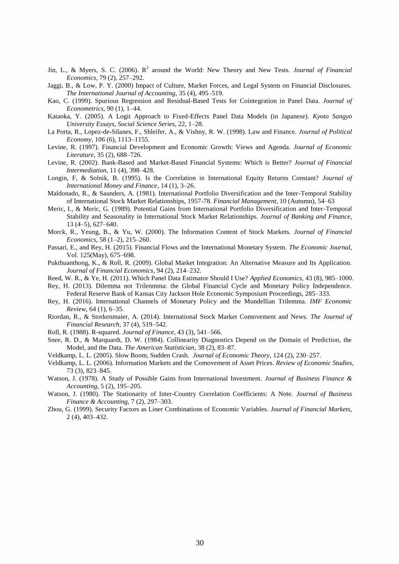
30

Jin, L., & Myers, S. C. (2006). R2 around the World: New Theory and New Tests. Journal of Financial

Economics, 79 (2), 257–292.

Jaggi, B., & Low, P. Y. (2000) Impact of Culture, Market Forces, and Legal System on Financial Disclosures.

The International Journal of Accounting, 35 (4), 495–519.

Kao, C. (1999). Spurious Regression and Residual-Based Tests for Cointegration in Panel Data. Journal of

Econometrics, 90 (1), 1–44.

Kataoka, Y. (2005). A Logit Approach to Fixed-Effects Panel Data Models (in Japanese). Kyoto Sangyo

University Essays, Social Science Series, 22, 1–28.

La Porta, R., Lopez-de-Silanes, F., Shleifer, A., & Vishny, R. W. (1998). Law and Finance. Journal of Political

Economy, 106 (6), 1113–1155.

Levine, R. (1997). Financial Development and Economic Growth: Views and Agenda. Journal of Economic

Literature, 35 (2), 688–726.

Levine, R. (2002). Bank-Based and Market-Based Financial Systems: Which is Better? Journal of Financial

Intermediation, 11 (4), 398–428.

Longin, F, & Solnik, B. (1995). Is the Correlation in International Equity Returns Constant? Journal of

International Money and Finance, 14 (1), 3–26.

Maldonado, R., & Saunders, A. (1981). International Portfolio Diversification and the Inter-Temporal Stability

of International Stock Market Relationships, 1957-78. Financial Management, 10 (Autumn), 54–63

Meric, I., & Meric, G. (1989). Potential Gains from International Portfolio Diversification and Inter-Temporal

Stability and Seasonality in International Stock Market Relationships. Journal of Banking and Finance,

13 (4–5), 627–640.

Morck, R., Yeung, B., & Yu, W. (2000). The Information Content of Stock Markets. Journal of Financial

Economics, 58 (1–2), 215–260.

Passari, E., and Rey, H. (2015). Financial Flows and the International Monetary System. The Economic Journal,

Vol. 125(May), 675–698.

Pukthuanthong, K., & Roll, R. (2009). Global Market Integration: An Alternative Measure and Its Application.

Journal of Financial Economics, 94 (2), 214–232.

Reed, W. R., & Ye, H. (2011). Which Panel Data Estimator Should I Use? Applied Economics, 43 (8), 985–1000.

Rey, H. (2013). Dilemma not Trilenmma: the Global Financial Cycle and Monetary Policy Independence.

Federal Reserve Bank of Kansas City Jackson Hole Economic Symposium Proceedings, 285–333.

Rey, H. (2016). International Channels of Monetary Policy and the Mundellian Trilemma. IMF Economic

Review, 64 (1), 6–35.

Riordan, R., & Storkenmaier, A. (2014). International Stock Market Comovement and News. The Journal of

Financial Research, 37 (4), 519–542.

Roll, R. (1988). R-squared. Journal of Finance, 43 (3), 541–566.

Snee, R. D., & Marquardt, D. W. (1984). Collinearity Diagnostics Depend on the Domain of Prediction, the

Model, and the Data. The American Statistician, 38 (2), 83–87.

Veldkamp, L. L. (2005). Slow Boom, Sudden Crash. Journal of Economic Theory, 124 (2), 230–257.

Veldkamp, L. L. (2006). Information Markets and the Comovement of Asset Prices. Review of Economic Studies,

73 (3), 823–845.

Watson, J. (1978). A Study of Possible Gains from International Investment. Journal of Business Finance &

Accounting, 5 (2), 195–205.

Watson, J. (1980). The Stationarity of Inter-Country Correlation Coefficients: A Note. Journal of Business

Finance & Accounting, 7 (2), 297–303.

Zhou, G. (1999). Security Factors as Liner Combinations of Economic Variables. Journal of Financial Markets,

2 (4), 403–432.

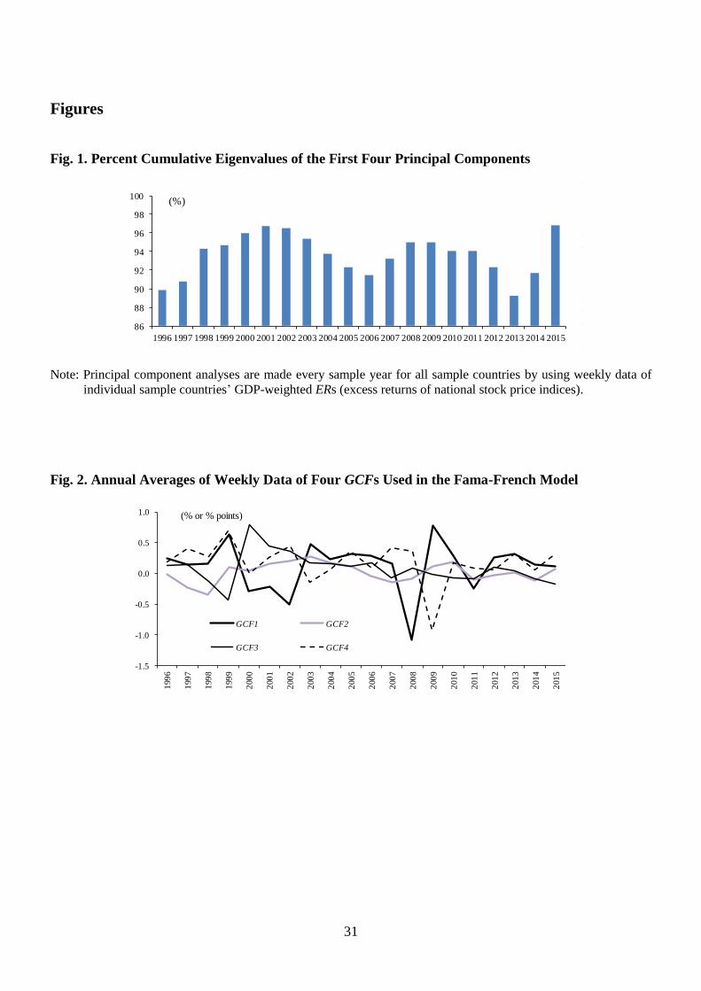
31

Figures

Fig. 1. Percent Cumulative Eigenvalues of the First Four Principal Components

Note: Principal component analyses are made every sample year for all sample countries by using weekly data of

individual sample countries’ GDP-weighted ERs (excess returns of national stock price indices).

Fig. 2. Annual Averages of Weekly Data of Four GCFs Used in the Fama-French Model

86

88

90

92

94

96

98

100

1996 1997 1998 1999 2000 2001 2002 2003 2004 2005 2006 2007 2008 2009 2010 2011 2012 2013 2014 2015

(%)

-1.5

-1.0

-0.5

0.0

0.5

1.0

199

6

199

7

199

8

199

9

200

0

200

1

200

2

200

3

200

4

200

5

200

6

200

7

200

8

200

9

201

0

201

1

201

2

201

3

201

4

201

5

GCF1 GCF2

GCF3 GCF4

(% or % points)

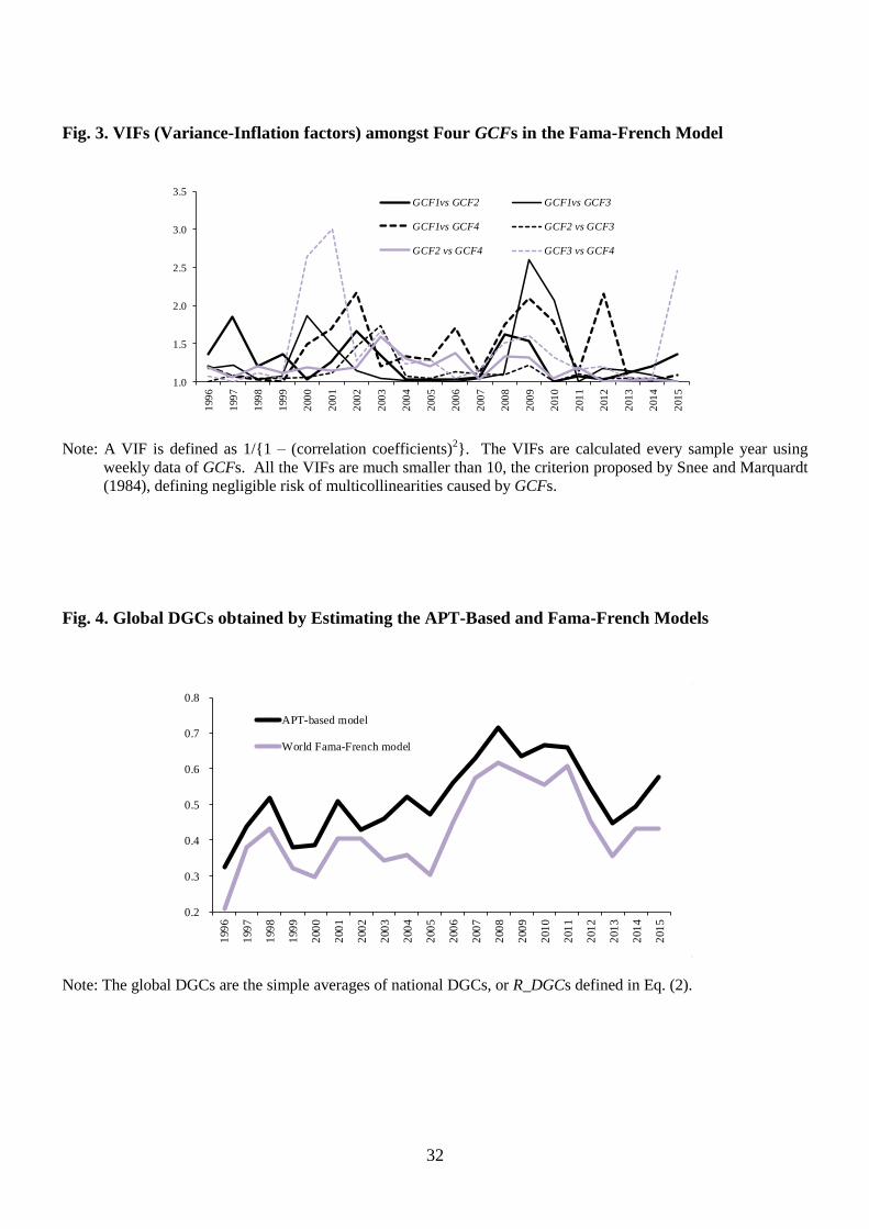
32

Fig. 3. VIFs (Variance-Inflation factors) amongst Four GCFs in the Fama-French Model

Note: A VIF is defined as 1/{1 – (correlation coefficients)

2}. The VIFs are calculated every sample year using

weekly data of GCFs. All the VIFs are much smaller than 10, the criterion proposed by Snee and Marquardt

(1984), defining negligible risk of multicollinearities caused by GCFs.

Fig. 4. Global DGCs obtained by Estimating the APT-Based and Fama-French Models

Note: The global DGCs are the simple averages of national DGCs, or R_DGCs defined in Eq. (2).

1.0

1.5

2.0

2.5

3.0

3.5

199

6

199

7

199

8

199

9

200

0

200

1

200

2

200

3

200

4

200

5

200

6

200

7

200

8

200

9

201

0

201

1

201

2

201

3

201

4

201

5

GCF1vs GCF2 GCF1vs GCF3

GCF1vs GCF4 GCF2 vs GCF3

GCF2 vs GCF4 GCF3 vs GCF4

0.2

0.3

0.4

0.5

0.6

0.7

0.8

199

6

199

7

199

8

199

9

200

0

200

1

200

2

200

3

200

4

200

5

200

6

200

7

200

8

200

9

201

0

201

1

201

2

201

3

201

4

201

5

APT-based model

World Fama-French model

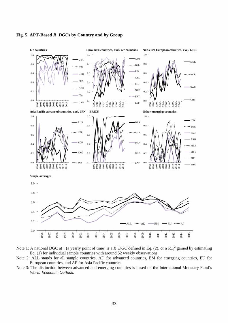
33

Fig. 5. APT-Based R_DGCs by Country and by Group

Note 1: A national DGC at τ (a yearly point of time) is a R_DGC defined in Eq. (2), or a Radj2 gained by estimating

Eq. (1) for individual sample countries with around 52 weekly observations.

Note 2: ALL stands for all sample countries, AD for advanced countries, EM for emerging countries, EU for

European countries, and AP for Asia Pacific countries.

Note 3: The distinction between advanced and emerging countries is based on the International Monetary Fund’s

World Economic Outlook.

G7 countries Euro area countries, excl. G7 countries Non-euro European countries, excl. GBR

Asia Pacific advanced countries, excl. JPN BRICS Other emerging countries

Simple averages

0.0

0.2

0.4

0.6

0.8

1.0

1996

1998

2000

2002

2004

2006

2008

2010

2012

2014

USA

JPN

GBR

FRA

DEU

ITA

CAN0.0

0.2

0.4

0.6

0.8

1.0

19

96

19

98

20

00

20

02

20

04

20

06

20

08

20

10

20

12

20

14

AUT

BEL

FIN

GRC

IRL

NLD

PRT

ESP0.0

0.2

0.4

0.6

0.8

1.0

19

96

19

98

20

00

20

02

20

04

20

06

20

08

20

10

20

12

20

14

DNK

NOR

SWE

CHE

0.0

0.2

0.4

0.6

0.8

1.0

1996

1998

2000

2002

2004

2006

2008

2010

2012

2014

BRA

RUS

IND

CHN

ZAF0.0

0.2

0.4

0.6

0.8

1.0

1996

1998

2000

2002

2004

2006

2008

2010

2012

2014

AUS

NZL

KOR

HKG

SGP 0.0

0.2

0.4

0.6

0.8

1.0

1996

1998

2000

2002

2004

2006

2008

2010

2012

2014

IDN

TUR

SAU

ARG

MEX

MYS

PHL

THA

0.0

0.2

0.4

0.6

0.8

1.0

19

96

19

97

19

98

19

99

20

00

20

01

20

02

20

03

20

04

20

05

20

06

20

07

20

08

20

09

20

10

20

11

20

12

20

13

20

14

20

15

ALL AD EM EU AP

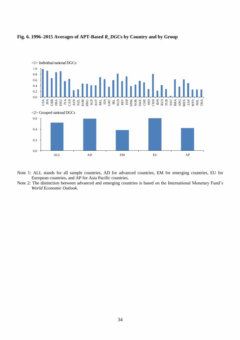
34

Fig. 6. 1996–2015 Averages of APT-Based R_DGCs by Country and by Group

Note 1: ALL stands for all sample countries, AD for advanced countries, EM for emerging countries, EU for

European countries, and AP for Asia Pacific countries.

Note 2: The distinction between advanced and emerging countries is based on the International Monetary Fund’s

World Economic Outlook.

<1> Individual national DGCs

<2> Grouped national DGCs

0.0

0.2

0.4

0.6

0.8

1.0

US

A

JPN

GB

R

FR

A

DE

U

ITA

CA

N

AU

S

NZ

L

KO

R

HK

G

SG

P

AU

T

BE

L

FIN

GR

C

IRL

NL

D

PR

T

ES

P

DN

K

NO

R

SW

E

CH

E

IND

CH

N

IDN

RU

S

TU

R

SA

U

BR

A

AR

G

ME

X

ZA

F

MY

S

PH

L

TH

A

0.0

0.2

0.4

0.6

ALL AD EM EU AP

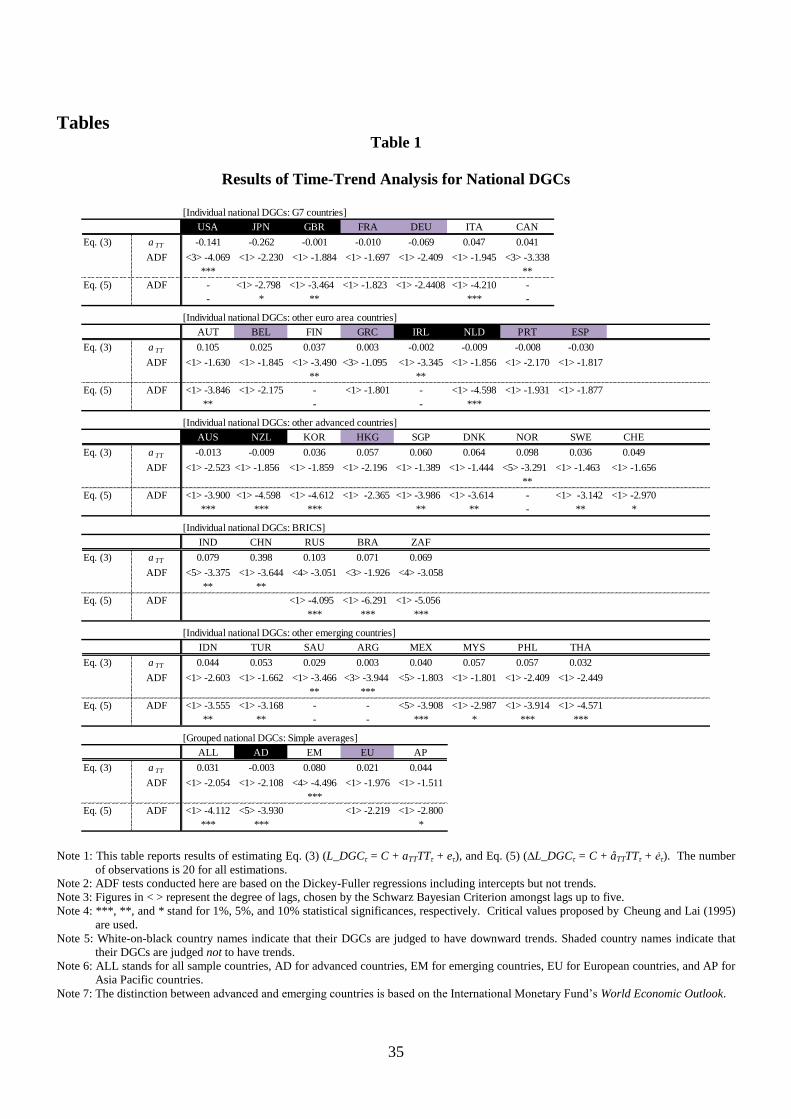
35

Tables Table 1

Results of Time-Trend Analysis for National DGCs

Note 1: This table reports results of estimating Eq. (3) (L_DGCτ = C + aTTTTτ + eτ), and Eq. (5) (∆L_DGCτ = C + åTTTTτ + ėτ). The number

of observations is 20 for all estimations.

Note 2: ADF tests conducted here are based on the Dickey-Fuller regressions including intercepts but not trends.

Note 3: Figures in < > represent the degree of lags, chosen by the Schwarz Bayesian Criterion amongst lags up to five.

Note 4: ***, **, and * stand for 1%, 5%, and 10% statistical significances, respectively. Critical values proposed by Cheung and Lai (1995)

are used.

Note 5: White-on-black country names indicate that their DGCs are judged to have downward trends. Shaded country names indicate that

their DGCs are judged not to have trends.

Note 6: ALL stands for all sample countries, AD for advanced countries, EM for emerging countries, EU for European countries, and AP for

Asia Pacific countries.

Note 7: The distinction between advanced and emerging countries is based on the International Monetary Fund’s World Economic Outlook.

[Individual national DGCs: G7 countries]

USA JPN GBR FRA DEU ITA CAN

Eq. (3) a TT -0.141 -0.262 -0.001 -0.010 -0.069 0.047 0.041

ADF <3> -4.069 <1> -2.230 <1> -1.884 <1> -1.697 <1> -2.409 <1> -1.945 <3> -3.338

*** **

Eq. (5) ADF - <1> -2.798 <1> -3.464 <1> -1.823 <1> -2.4408 <1> -4.210 -

- * ** *** -

[Individual national DGCs: other euro area countries]

AUT BEL FIN GRC IRL NLD PRT ESP

Eq. (3) a TT 0.105 0.025 0.037 0.003 -0.002 -0.009 -0.008 -0.030

ADF <1> -1.630 <1> -1.845 <1> -3.490 <3> -1.095 <1> -3.345 <1> -1.856 <1> -2.170 <1> -1.817

** **

Eq. (5) ADF <1> -3.846 <1> -2.175 - <1> -1.801 - <1> -4.598 <1> -1.931 <1> -1.877

** - - ***

[Individual national DGCs: other advanced countries]

AUS NZL KOR HKG SGP DNK NOR SWE CHE

Eq. (3) a TT -0.013 -0.009 0.036 0.057 0.060 0.064 0.098 0.036 0.049

ADF <1> -2.523 <1> -1.856 <1> -1.859 <1> -2.196 <1> -1.389 <1> -1.444 <5> -3.291 <1> -1.463 <1> -1.656

**

Eq. (5) ADF <1> -3.900 <1> -4.598 <1> -4.612 <1> -2.365 <1> -3.986 <1> -3.614 - <1> -3.142 <1> -2.970

*** *** *** ** ** - ** *

[Individual national DGCs: BRICS]

IND CHN RUS BRA ZAF

Eq. (3) a TT 0.079 0.398 0.103 0.071 0.069

ADF <5> -3.375 <1> -3.644 <4> -3.051 <3> -1.926 <4> -3.058

** **

Eq. (5) ADF <1> -4.095 <1> -6.291 <1> -5.056

*** *** ***

[Individual national DGCs: other emerging countries]

IDN TUR SAU ARG MEX MYS PHL THA

Eq. (3) a TT 0.044 0.053 0.029 0.003 0.040 0.057 0.057 0.032

ADF <1> -2.603 <1> -1.662 <1> -3.466 <3> -3.944 <5> -1.803 <1> -1.801 <1> -2.409 <1> -2.449

** ***

Eq. (5) ADF <1> -3.555 <1> -3.168 - - <5> -3.908 <1> -2.987 <1> -3.914 <1> -4.571

** ** - - *** * *** ***

[Grouped national DGCs: Simple averages]

ALL AD EM EU AP

Eq. (3) a TT 0.031 -0.003 0.080 0.021 0.044

ADF <1> -2.054 <1> -2.108 <4> -4.496 <1> -1.976 <1> -1.511

***

Eq. (5) ADF <1> -4.112 <5> -3.930 <1> -2.219 <1> -2.800

*** *** *

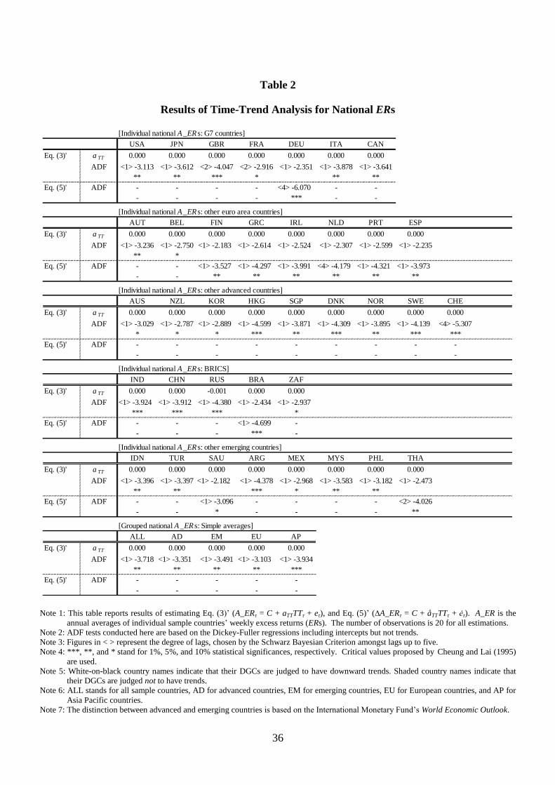
36

Table 2

Results of Time-Trend Analysis for National ERs

Note 1: This table reports results of estimating Eq. (3)’ (A_ERτ = C + aTTTTτ + eτ), and Eq. (5)’ (∆A_ERτ = C + åTTTTτ + ėτ). A_ER is the

annual averages of individual sample countries’ weekly excess returns (ERs). The number of observations is 20 for all estimations.

Note 2: ADF tests conducted here are based on the Dickey-Fuller regressions including intercepts but not trends.

Note 3: Figures in < > represent the degree of lags, chosen by the Schwarz Bayesian Criterion amongst lags up to five.

Note 4: ***, **, and * stand for 1%, 5%, and 10% statistical significances, respectively. Critical values proposed by Cheung and Lai (1995)

are used.

Note 5: White-on-black country names indicate that their DGCs are judged to have downward trends. Shaded country names indicate that

their DGCs are judged not to have trends.

Note 6: ALL stands for all sample countries, AD for advanced countries, EM for emerging countries, EU for European countries, and AP for

Asia Pacific countries.

Note 7: The distinction between advanced and emerging countries is based on the International Monetary Fund’s World Economic Outlook.

[Individual national A_ER s: G7 countries]

USA JPN GBR FRA DEU ITA CAN

Eq. (3)' a TT 0.000 0.000 0.000 0.000 0.000 0.000 0.000

ADF <1> -3.113 <1> -3.612 <2> -4.047 <2> -2.916 <1> -2.351 <1> -3.878 <1> -3.641

** ** *** * ** **

Eq. (5)' ADF - - - - <4> -6.070 - -

- - - - *** - -

[Individual national A_ER s: other euro area countries]

AUT BEL FIN GRC IRL NLD PRT ESP

Eq. (3)' a TT 0.000 0.000 0.000 0.000 0.000 0.000 0.000 0.000

ADF <1> -3.236 <1> -2.750 <1> -2.183 <1> -2.614 <1> -2.524 <1> -2.307 <1> -2.599 <1> -2.235

** *

Eq. (5)' ADF - - <1> -3.527 <1> -4.297 <1> -3.991 <4> -4.179 <1> -4.321 <1> -3.973

- - ** ** ** ** ** **

[Individual national A_ER s: other advanced countries]

AUS NZL KOR HKG SGP DNK NOR SWE CHE

Eq. (3)' a TT 0.000 0.000 0.000 0.000 0.000 0.000 0.000 0.000 0.000

ADF <1> -3.029 <1> -2.787 <1> -2.889 <1> -4.599 <1> -3.871 <1> -4.309 <1> -3.895 <1> -4.139 <4> -5.307

* * * *** ** *** ** *** ***

Eq. (5)' ADF - - - - - - - - -

- - - - - - - - -

[Individual national A_ER s: BRICS]

IND CHN RUS BRA ZAF

Eq. (3)' a TT 0.000 0.000 -0.001 0.000 0.000

ADF <1> -3.924 <1> -3.912 <1> -4.380 <1> -2.434 <1> -2.937

*** *** *** *

Eq. (5)' ADF - - - <1> -4.699 -

- - - *** -

[Individual national A_ER s: other emerging countries]

IDN TUR SAU ARG MEX MYS PHL THA

Eq. (3)' a TT 0.000 0.000 0.000 0.000 0.000 0.000 0.000 0.000

ADF <1> -3.396 <1> -3.397 <1> -2.182 <1> -4.378 <1> -2.968 <1> -3.583 <1> -3.182 <1> -2.473

** ** *** * ** **

Eq. (5)' ADF - - <1> -3.096 - - - - <2> -4.026

- - * - - - - **

[Grouped national A_ER s: Simple averages]

ALL AD EM EU AP

Eq. (3)' a TT 0.000 0.000 0.000 0.000 0.000

ADF <1> -3.718 <1> -3.351 <1> -3.491 <1> -3.103 <1> -3.934

** ** ** ** ***

Eq. (5)' ADF - - - - -

- - - - -

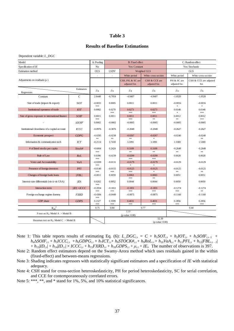
37

Table 3

Results of Baseline Estimations

Note 1: This table reports results of estimating Eq. (6): L_DGCi,τ = C + h1SOTi,τ + h2IOTi,τ + h3SOIFi,τ–1 +

h4∆SOIFi,τ + h5ICCCi,τ + h6GDPGi,τ + h7ICTi,τ+ h8STOCK#i,τ + h9RoLi,τ + h10VaAi,τ + h11PFIi,τ + h12|FBLi,τ – 1| + h13|IDi,τ| + h14|IDi,τ| × ICCCi,τ + h15FXRDi,τ + h16GDPSi,τ + μi,τ + IEi. The number of observations is 397.

Note 2: Random effect estimators depend on the Swamy-Arora method which uses residuals gained in the within

(fixed-effect) and between-means regressions.

Note 3: Shading indicates regressors with statistically significant estimators and a specification of IE with statistical

adequacy.

Note 4: CSH stand for cross-section heteroskedasticity, PH for period heteroskedasticity, SC for serial correlation,

and CCE for contemporaneously correlated errors.

Note 5: ***, **, and * stand for 1%, 5%, and 10% statistical significances.

Dependent variable: L_DGC

Model A: Pooling

Specification of IE No

Estimation method OLS LSDV

- - White period White cross-section White period White cross-section

CSH, PH, & SC are

adjusted for.

CSH & CCE are

adjusted for.

PH & SC are

adjusted for.

CSH & CCE are adjusted

for.

ĥ s ĥ s ĥ s ĥ s ĥ s ĥ s

Constant C 2.6448 -6.7054 -4.9407 -4.9407 -1.0520 -1.0520

Size of trade (import & export) SOT -0.0031 0.0005 0.0011 0.0011 -0.0016 -0.0016

*** * *

Institutional openness of trade IOT 0.0082 0.0270 0.0273 0.0273 0.0148 0.0148

*** *** *** * ***

Size of gross exposure to international finance SOIF 0.0015 0.0011 0.0011 0.0011 0.0012 0.0012

*** *** ** ** ***

- ∆SOIF 0.0002 -0.0002 -0.0005 -0.0005 -0.0005 -0.0005

Institutional closedness of a capital account ICCC -0.0976 -0.3876 -0.2049 -0.2049 -0.2627 -0.2627

Economic prospect GDPG -0.0295 -0.0238 -0.0267 -0.0267 -0.0240 -0.0240

** ** ** * **

Information & communication tech ICT -0.2114 3.7418 3.1091 3.1091 1.5369 1.5369

# of listed stocks per capita Stock# -0.6004 0.2424 0.3109 0.3109 -0.2648 -0.2648

*** ** ** ** **

Rule of Law RoL 0.0396 -0.0239 -0.0299 -0.0299 0.0028 0.0028

*** *** ***

Voice and Accountability VaA -0.0209 -0.0131 -0.0179 -0.0179 -0.0129 -0.0129

*** * *

Presence of foreign investors PFI -0.0140 -0.0155 -0.0125 -0.0125 -0.0125 -0.0125

*** *** *** * ** **

Changes of foreign bank loans |FBL| -0.0011 0.0059 0.0063 0.0063 0.0051 0.0051

*** **

Interest-rate differentials (vis-à-vis USA) |ID| 0.0202 0.0052 0.0044 0.0044 0.0050 0.0050

***

Interaction term |ID| ×ICCC -0.2054 -0.1651 -0.1831 -0.1831 -0.1274 -0.1274

*** *** *** *** *** **

Foreign exchange regime dummy FXRD -0.4384 -0.0449 -0.0875 -0.0875 -0.1160 -0.1160

***

GDP share GDPS 0.2327 0.3599 0.4031 0.4031 0.2856 0.2856

*** *** *** *** *** ***

0.75 0.84Radj2 0.77 0.44

B: Fixed effect C: Random effect

Yes: Constant Yes: Stochastic

Weighted GLS GLS

Hausman test on H0: Model C > Model B52.39

(p-value: 0.00)

Adjustments on residuals (μ )

F-test on H0: Model A > Model B7.77

(p-value: 0.00)

Regressors

Estimators

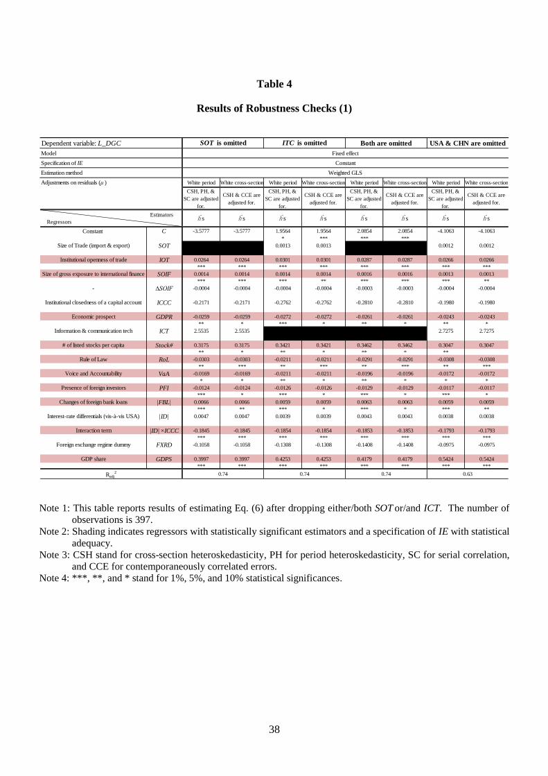
38

Table 4

Results of Robustness Checks (1)

Note 1: This table reports results of estimating Eq. (6) after dropping either/both SOT or/and ICT. The number of

observations is 397.

Note 2: Shading indicates regressors with statistically significant estimators and a specification of IE with statistical

adequacy.

Note 3: CSH stand for cross-section heteroskedasticity, PH for period heteroskedasticity, SC for serial correlation,

and CCE for contemporaneously correlated errors.

Note 4: ***, **, and * stand for 1%, 5%, and 10% statistical significances.

Dependent variable: L_DGC

Model

Specification of IE

Estimation method

Adjustments on residuals (μ ) White period White cross-section White period White cross-section White period White cross-section White period White cross-section

CSH, PH, &

SC are adjusted

for.

CSH & CCE are

adjusted for.

CSH, PH, &

SC are adjusted

for.

CSH & CCE are

adjusted for.

CSH, PH, &

SC are adjusted

for.

CSH & CCE are

adjusted for.

CSH, PH, &

SC are adjusted

for.

CSH & CCE are

adjusted for.

ĥ s ĥ s ĥ s ĥ s ĥ s ĥ s ĥ s ĥ s

Constant C -3.5777 -3.5777 1.9564 1.9564 2.0854 2.0854 -4.1063 -4.1063

* *** *** ***

Size of Trade (import & export) SOT 0.0013 0.0013 0.0012 0.0012

Institutional openness of trade IOT 0.0264 0.0264 0.0301 0.0301 0.0287 0.0287 0.0266 0.0266

*** *** *** *** *** *** *** ***

Size of gross exposure to international finance SOIF 0.0014 0.0014 0.0014 0.0014 0.0016 0.0016 0.0013 0.0013

*** *** *** ** *** *** *** **

- ∆SOIF -0.0004 -0.0004 -0.0004 -0.0004 -0.0003 -0.0003 -0.0004 -0.0004

Institutional closedness of a capital account ICCC -0.2171 -0.2171 -0.2762 -0.2762 -0.2810 -0.2810 -0.1980 -0.1980

Economic prospect GDPR -0.0259 -0.0259 -0.0272 -0.0272 -0.0261 -0.0261 -0.0243 -0.0243

** * *** * ** * ** *

Information & communication tech ICT 2.5535 2.5535 2.7275 2.7275

# of listed stocks per capita Stock# 0.3175 0.3175 0.3421 0.3421 0.3462 0.3462 0.3047 0.3047

** * ** * ** * **

Rule of Law RoL -0.0303 -0.0303 -0.0211 -0.0211 -0.0291 -0.0291 -0.0308 -0.0308

** *** ** *** ** *** ** ***

Voice and Accountability VaA -0.0169 -0.0169 -0.0211 -0.0211 -0.0196 -0.0196 -0.0172 -0.0172

* * ** * ** * * *

Presence of foreign investors PFI -0.0124 -0.0124 -0.0126 -0.0126 -0.0129 -0.0129 -0.0117 -0.0117

*** * *** * *** * *** *

Changes of foreign bank loans |FBL| 0.0066 0.0066 0.0059 0.0059 0.0063 0.0063 0.0059 0.0059

*** ** *** * *** * *** **

Interest-rate differentials (vis-à-vis USA) |ID| 0.0047 0.0047 0.0039 0.0039 0.0043 0.0043 0.0038 0.0038

Interaction term |ID| ×ICCC -0.1845 -0.1845 -0.1854 -0.1854 -0.1853 -0.1853 -0.1793 -0.1793

*** *** *** *** *** *** *** ***

Foreign exchange regime dummy FXRD -0.1058 -0.1058 -0.1308 -0.1308 -0.1408 -0.1408 -0.0975 -0.0975

GDP share GDPS 0.3997 0.3997 0.4253 0.4253 0.4179 0.4179 0.5424 0.5424

*** *** *** *** *** *** *** ***

Radj2 0.74 0.74 0.63

SOT is omitted ITC is omitted USA & CHN are omitted

Fixed effect

Constant

Weighted GLS

0.74

Both are omitted

Regressors

Estimators

39

Table 5

Results of Robustness Checks (2)

Note 1: This table reports results of estimating the following equation: L_DGCi,τ = C + h1SOTi,τ + h2IOTi, τ – 1 +

h3SOIFi,τ – 1 + h4∆SOIFi,τ + h5ICCCi,τ + h6GDPGi,τ + h7ICTi,τ+ h8STOCK#i, τ + h9RoLi,τ + h10VaAi,τ + h11PFIi,τ

+ h12|FBLi,τ – 1| + h13|IDi,τ| + h14|IDi,τ| × ICCCi,τ + h15FXRDi,τ + h16GDPSi,τ + μi,τ + IEi. The number of

observations is 397.

Note 2: Random effect estimators depend on the Swamy-Arora method which uses residuals gained in the within

(fixed-effect) and between-means regressions.

Note 3: Shading indicates regressors with statistically significant estimators and a specification of IE with statistical

adequacy.

Note 4: CSH stand for cross-section heteroskedasticity, PH for period heteroskedasticity, SC for serial correlation,

and CCE for contemporaneously correlated errors.

Note 5: ***, **, and * stand for 1%, 5%, and 10% statistical significances.

Dependent variable: L_DGC

Model A: Pooling

Specification of IE No

Estimation method OLS LSDV

- - White period White cross-section White period White cross-section

CSH, PH, & SC are

adjusted for.

CSH & CCE are

adjusted for.

PH & SC are

adjusted for.

CSH & CCE are adjusted

for.

ĥ s ĥ s ĥ s ĥ s ĥ s ĥ s

Constant C 2.7792 -4.9810 -1.8592 -1.8592 -0.7577 -0.7577

Size of trade (import & export) SOT -0.0032 0.0004 0.0009 0.0009 -0.0017 -0.0017

***

Institutional openness of trade IOT τ – 1 0.0083 0.0272 0.0272 0.0272 0.0141 0.0141

*** *** *** * ***

Size of gross exposure to international finance SOIF 0.0015 0.0012 0.0013 0.0013 0.0012 0.0012

*** *** ** ** ***

- ∆SOIF -0.0001 0.0000 -0.0002 -0.0002 -0.0004 -0.0004

Institutional closedness of a capital account ICCC -0.1088 -0.5132 -0.4088 -0.4088 -0.3139 -0.3139

Economic prospect GDPR -0.0290 -0.0207 -0.0238 -0.0238 -0.0225 -0.0225

** *

Information & communication tech ICT -0.2757 3.0894 1.8831 1.8831 1.4342 1.4342

# of listed stocks per capita Stock# -0.6008 0.2573 0.3156 0.3156 -0.2661 -0.2661

*** ** * **

Rule of Law RoL 0.0400 -0.0233 -0.0279 -0.0279 0.0037 0.0037

*** * ** ***

Voice and Accountability VaA -0.0210 -0.0194 -0.0232 -0.0232 -0.0136 -0.0136

*** * ** **

Presence of foreign investors PFI -0.0141 -0.0173 -0.0123 -0.0123 -0.0125 -0.0125

*** *** ** *** **

Changes of foreign bank loans |FBL| -0.0008 -0.0151 -0.0067 -0.0067 0.0056 0.0056

*** *** ** *

Interest-rate differentials (vis-à-vis USA) |ID| 0.0200 0.0046 -0.0036 -0.0036 0.0048 0.0048

Interaction term |ID| ×ICCC -0.2036 -0.1602 -0.1752 -0.1752 -0.1229 -0.1229

*** ** *** *** *** ***

Foreign exchange regime dummy FXRD -0.4371 -0.0660 -0.1280 -0.1280 -0.1150 -0.1150

***

GDP share GDPS 0.2324 0.3637 0.4130 0.4130 0.2853 0.2853

*** *** *** *** *** ***

0.75 0.84

Hausman test on H0: Model C > Model B53.12

(p-value: 0.00)

Adjustments on residuals (μ )

Radj2 0.74 0.42

F-test on H0: Model A > Model B7.81

(p-value: 0.00)

Weighted GLS GLS

B: Fixed effect C: Random effect

Yes: Constant Yes: Stochastic

Regressors

Estimators

40

Table C1

Definitions and Sources of Data Used

Indicators Notations Definitions Sources Notes

National economic

size.GDPS Percentages of nominal GDP in world GDP.

IMF, World

Economic

Outlook

(WEO).

In U.S. dollar volume.

Excess returns of

national stock.ER

{(National stock prices at t / National stock prices at t-1 ) – 1

week interest rates of US dollar at t-1}.Bloomberg

% points. National stock pirces

are quoted in U.S. dollar. The

interest rates are linearly

interpolated with FF effective

rates and 1-year Treasury bill

yields.

National stock

prices.-

Argentina Merval Index for ARG, All Ordinaries Index for AUS,

MSCI Austria for AUT, Belgian All-Share Index for BEL, MSCI

Brazil for BRA, S&P/Toronto Stock Exchange Composite Index

for CAN, Shanghai Stock Exchange Composite Index for CHN,

OMX Copenhagen 20 for DNK, OMX Helsinki All-Share Index

for FIN, CAC All-Tradable for FRA, HDAX for DEU, Athex

Composite Share Price Index for GRC, Hang Seng Index for HKG,

Standard &Poor's BSE Sensex Index for IND, Jakarta Composite

Index for IDN, ISEQ All-Share Index for Ireland, MSCI Italy for

ITA, Tokyo Stock Price Index for JPN, FTSE Bursa Malaysia

EMAS Index for MYS, MSCI Mexico for MEX, AEX for NLD,

MSCI New Zealand for NZL, OBX for NOR, PSEi Index for PHL,

PSI All-Share Index for PRT, CS First Boston Russian Stock

Market Index for RUS, Tadawul All-Share Index for SAU, MSCI

Singapore for SGP, FTSE/JSE Africa All Shares for ZAF, Korea

Composite Stock Price Index for KOR, Madrid Stock Exchange

General Index for ESP, OMX Stockholm 30 for SWE, Swiss

Market Index for CHE, Bangkok SET Index for THA, Borsa

Istanbul 100 for TUR, FTSE All-Share Index for GBR, and

Standard & Poor's 500 for USA.

See the above. In U.S. dollar value.

Market factor.Fama-French

GCF1GDP-weighted averages of 37 countries' ER s. See the above.

% points. Nominal GDPs are

taken from IMF, WEO. This is

applicable to all indicators

divided by nominal GDPs.

Size factor.Fama-French

GCF2

A global portfolio is a market-capitalisation weighted sum of

liquid corporate stock prices in 23 advanced countries. All stocks

are sorted into big and small stocks by market capitalisation. Big

stocks are those in the top 90% whilst small stocks are those in the

bottom 10%. Stocks in each stock group are sorted into three sub-

groups by three ratios gained by dividing (i) market equity, (ii)

operating profits, and (iii) changes of total assets by book equity.

Stocks in each sub-group are classified in to bottom 30%, middle

40%, and top 10%. As a result, big stocks consist of nine

portfolios, and so do small stocks. SMB is the average excess

return on the nine small portfolios minus the average excess return

on the nine big portfolios.

Fama/French

Global 5

Factors

[Daily]

% points.

Value factor.Fama-French

GCF3

HML = 1/2(Excess return on small stocks with bottom-30% book-

to-market equity ratios + excess return on big stocks with bottom-

30% book-to-market equity ratios) – 1/2(Excess return on small

stocks with top-10% book-to-market equity ratios + excess return

on big stocks with top-10% book-to-market equity ratios).

See the above. See the above.

Momentum factor.Fama-French

GCF4

WML (the difference between the returns on diversified portfolios

of top-30% strong stocks and bottom-30% weak stocks) .

Fama/French

Global

Momentum

Factor (Mom)

[Daily]

See the above.

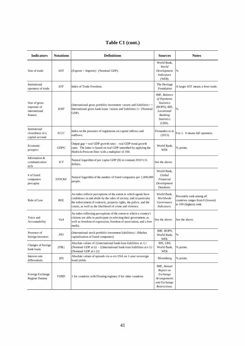
41

Table C1 (cont.)

Indicators Notations Definitions Sources Notes

Size of trade SOT (Exports + Imports) / (Nominal GDP).

World Bank,

World

Development

Indicators

(WDI).

%

Institutional

openness of trade.IOT Index of Trade Freedom.

The Heritage

FoundationA larger IOT means a freer trade.

Size of gross

exposure of

international

finance.

SOIF

(International gross portfolio investment <assets and liabilities> +

International gross bank loans <assets and liabilities>) / (Nominal

GDP).

IMF, Balance

of Payments

Statistics

(BOPS); BIS,

Locational

Banking

Statistics

(LBS).

%

Institutional

closedness of a

capital account

ICCCIndex on the presence of regulations on capital inflows and

outflows.

Fernandez et al.

(2015)0 to 1. 0 means full openness.

Economic

prospectGDPG

Output gap = real GDP growth rates – real GDP trend growth

rates. The latter is based on real GDP smoothed by applying the

Hodrick-Prescott filter with a multiplier of 100.

World Bank,

WDI.% points.

Information &

communication

tech

ICTNatural logarithm of per capita GDP ($) in constant 2010 U.S.

dollars.See the above.

# of listed

companies

percapita

STOCK#Natural logarithm of the number of listed companies per 1,000,000

people.

World Bank,

Global

Financial

Development

Database.

Rule of Law ROL

An index reflects perceptions of the extent to which agents have

confidence in and abide by the rules of society, and in particuler

the enforcement of contracts, property rights, the police, and the

courts, as well as the likelihood of crime and violence.

World Bank,

Worldwide

Governance

Indicators.

Percentile rank among all

countries ranges from 0 (lowest)

to 100 (highest) rank.

Voice and

AccountabilityVaA

An index reflecting perceptions of the extent to which a country's

citizens are able to participate in selecting their government, as

well as freedom of expression, freedom of association, and a free

media.

See the above. See the above.

Presence of

foreign investorsPFI

(International stock portfolio investment liabilities) / (Market

capitalisation of listed companies)

IMF, BOPS;

World Bank,

WDI.

%

Changes of foreign

bank loans|FBL|

Absolute values of {(international bank-loan liabilities at t ) /

(Nominal GDP at t)} - {(International bank-loan liabilities at t-1) /

(Nominal GDP at t-1)}

BIS, LBS;

World Bank,

WDI.

% points.

Interest-rate

differentials|ID|

Absolute values of spreads vis-a-vis USA on 1-year sovereign

bond yields.Bloomberg % points.

Foreign Exchange

Regime DummyFXRD 1 for countries with Floating regimes; 0 for other countries

IMF, Annual

Report on

Exchange

Arrangements

and Exchange

Restrictions.

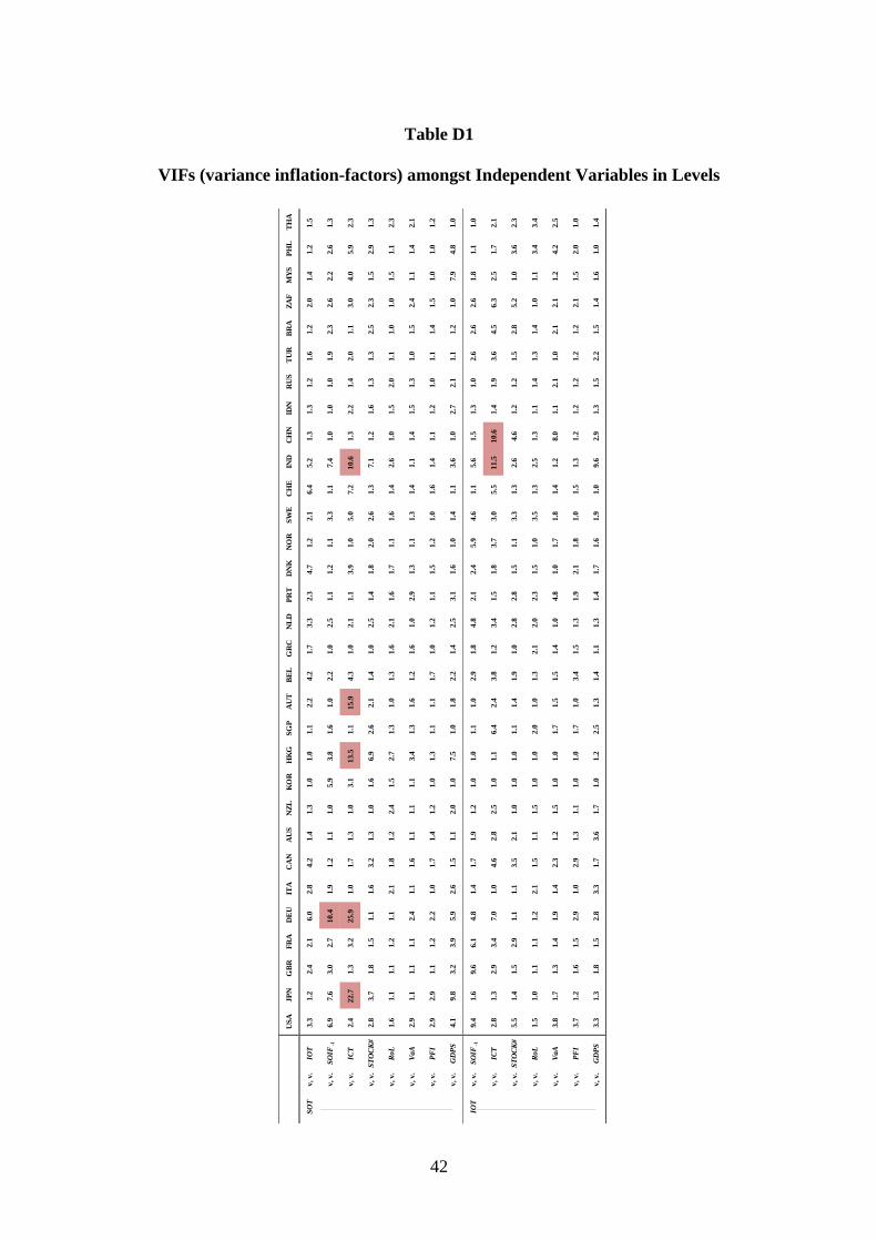
42

Table D1

VIFs (variance inflation-factors) amongst Independent Variables in Levels

US

AJP

NG

BR

FR

AD

EU

ITA

CA

NA

US

NZ

LK

OR

HK

GS

GP

AU

TB

EL

GR

CN

LD

PR

TD

NK

NO

RS

WE

CH

EIN

DC

HN

IDN

RU

ST

UR

BR

AZ

AF

MY

SP

HL

TH

A

SO

Tv, v.

IOT

3.3

1.2

2.4

2.1

6.0

2.8

4.2

1.4

1.3

1.0

1.0

1.1

2.2

4.2

1.7

3.3

2.3

4.7

1.2

2.1

6.4

5.2

1.3

1.3

1.2

1.6

1.2

2.0

1.4

1.2

1.5

v, v.

SO

IF-1

6.9

7.6

3.0

2.7

10.4

1.9

1.2

1.1

1.0

5.9

3.8

1.6

1.0

2.2

1.0

2.5

1.1

1.2

1.1

3.3

1.1

7.4

1.0

1.0

1.0

1.9

2.3

2.6

2.2

2.6

1.3

v, v.

ICT

2.4

22.7

1.3

3.2

25.9

1.0

1.7

1.3

1.0

3.1

13.5

1.1

15.9

4.3

1.0

2.1

1.1

3.9

1.0

5.0

7.2

10.6

1.3

2.2

1.4

2.0

1.1

3.0

4.0

5.9

2.3

v, v.

ST

OC

K#

2.8

3.7

1.8

1.5

1.1

1.6

3.2

1.3

1.0

1.6

6.9

2.6

2.1

1.4

1.0

2.5

1.4

1.8

2.0

2.6

1.3

7.1

1.2

1.6

1.3

1.3

2.5

2.3

1.5

2.9

1.3

v, v.

RoL

1.6

1.1

1.1

1.2

1.1

2.1

1.8

1.2

2.4

1.5

2.7

1.3

1.0

1.3

1.6

2.1

1.6

1.7

1.1

1.6

1.4

2.6

1.0

1.5

2.0

1.1

1.0

1.0

1.5

1.1

2.3

v, v.

VaA

2.9

1.1

1.1

1.1

2.4

1.1

1.6

1.1

1.1

1.1

3.4

1.3

1.6

1.2

1.6

1.0

2.9

1.3

1.1

1.3

1.4

1.1

1.4

1.5

1.3

1.0

1.5

2.4

1.1

1.4

2.1

v, v.

PF

I2.9

2.9

1.1

1.2

2.2

1.0

1.7

1.4

1.2

1.0

1.3

1.1

1.1

1.7

1.0

1.2

1.1

1.5

1.2

1.0

1.6

1.4

1.1

1.2

1.0

1.1

1.4

1.5

1.0

1.0

1.2

v, v.

GD

PS

4.1

9.8

3.2

3.9

5.9

2.6

1.5

1.1

2.0

1.0

7.5

1.0

1.8

2.2

1.4

2.5

3.1

1.6

1.0

1.4

1.1

3.6

1.0

2.7

2.1

1.1

1.2

1.0

7.9

4.8

1.0

IOT

v, v.

SO

IF-1

9.4

1.6

9.6

6.1

4.8

1.4

1.7

1.9

1.2

1.0

1.0

1.1

1.0

2.9

1.8

4.8

2.1

2.4

5.9

4.6

1.1

5.6

1.5

1.3

1.0

2.6

2.6

2.6

1.8

1.1

1.0

v, v.

ICT

2.8

1.3

2.9

3.4

7.0

1.0

4.6

2.8

2.5

1.0

1.1

6.4

2.4

3.8

1.2

3.4

1.5

1.8

3.7

3.0

5.5

11.5

10.6

1.4

1.9

3.6

4.5

6.3

2.5

1.7

2.1

v, v.

ST

OC

K#

5.5

1.4

1.5

2.9

1.1

1.1

3.5

2.1

1.0

1.0

1.0

1.1

1.4

1.9

1.0

2.8

2.8

1.5

1.1

3.3

1.3

2.6

4.6

1.2

1.2

1.5

2.8

5.2

1.0

3.6

2.3

v, v.

RoL

1.5

1.0

1.1

1.1

1.2

2.1

1.5

1.1

1.5

1.0

1.0

2.0

1.0

1.3

2.1

2.0

2.3

1.5

1.0

3.5

1.3

2.5

1.3

1.1

1.4

1.3

1.4

1.0

1.1

3.4

3.4

v, v.

VaA

3.8

1.7

1.3

1.4

1.9

1.4

2.3

1.2

1.5

1.0

1.0

1.7

1.5

1.5

1.4

1.0

4.8

1.0

1.7

1.8

1.4

1.2

8.0

1.1

2.1

1.0

2.1

2.1

1.2

4.2

2.5

v, v.

PF

I3.7

1.2

1.6

1.5

2.9

1.0

2.9

1.3

1.1

1.0

1.0

1.7

1.0

3.4

1.5

1.3

1.9

2.1

1.8

1.0

1.5

1.3

1.2

1.2

1.2

1.2

1.2

2.1

1.5

2.0

1.0

v, v.

GD

PS

3.3

1.3

1.8

1.5

2.8

3.3

1.7

3.6

1.7

1.0

1.2

2.5

1.3

1.4

1.1

1.3

1.4

1.7

1.6

1.9

1.0

9.6

2.9

1.3

1.5

2.2

1.5

1.4

1.6

1.0

1.4

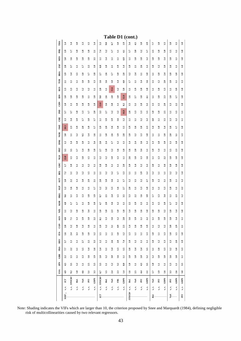
43

Table D1 (cont.)

Note: Shading indicates the VIFs which are larger than 10, the criterion proposed by Snee and Marquardt (1984), defining negligible

risk of multicollinearities caused by two relevant regressors.

US

AJ

PN

GB

RF

RA

DE

UIT

AC

AN

AU

SN

ZL

KO

RH

KG

SG

PA

UT

BE

LG

RC

NL

DP

RT

DN

KN

OR

SW

EC

HE

IND

CH

NID

NR

US

TU

RB

RA

ZA

FM

YS

PH

LT

HA

SO

IF-1

v, v.

ICT

4.9

4.5

2.2

7.7

5.7

1.6

2.0

4.8

1.1

4.8

9.6

1.2

1.0

7.2

1.7

13.8

3.5

1.2

3.0

10.3

1.3

5.7

1.0

1.0

1.3

2.1

1.9

2.8

5.0

1.9

1.4

v, v.

ST

OC

K#

9.2

3.5

1.5

2.2

1.1

2.4

1.2

7.1

1.2

1.7

5.1

1.6

2.2

1.1

1.0

1.5

3.5

1.4

1.1

2.3

1.4

3.7

1.1

1.0

1.3

1.1

1.4

3.7

1.6

1.7

1.4

v, v.

RoL

1.8

1.2

1.1

1.1

1.1

3.3

1.0

1.3

1.0

1.7

1.3

1.0

1.3

1.2

1.1

1.3

1.7

1.0

1.2

1.9

1.9

1.8

1.0

1.0

1.3

1.1

1.5

1.1

1.0

1.0

1.0

v, v.

VaA

4.6

1.1

1.3

1.5

2.7

1.0

1.4

1.9

1.0

1.1

1.3

1.1

1.0

1.2

1.1

1.0

1.4

1.0

9.5

2.0

1.7

1.3

1.0

1.0

1.2

1.0

1.0

1.7

1.0

1.0

1.3

v, v.

PF

I5.1

2.5

1.6

1.4

2.2

1.0

1.6

1.0

3.4

1.0

1.8

1.1

2.9

1.5

1.2

1.5

3.0

1.1

1.4

1.0

1.0

1.7

1.0

1.1

1.2

1.0

1.7

2.2

1.0

1.0

1.5

v, v.

GD

PS

3.3

5.5

1.9

1.6

3.3

1.2

1.1

2.2

1.1

1.0

1.9

1.7

2.1

1.1

1.1

1.1

1.0

3.4

1.6

1.7

1.7

2.0

1.0

1.0

1.1

1.3

1.8

1.0

3.5

2.1

1.4

ICT

v, v.

ST

OC

K#

6.7

3.3

1.0

1.4

1.2

1.5

1.9

8.1

1.0

4.7

9.7

1.2

2.0

1.1

1.8

1.2

2.7

2.0

1.1

1.9

1.1

3.3

13.8

9.0

2.0

1.6

2.7

6.8

1.1

7.4

5.3

v, v.

RoL

1.5

1.1

1.2

1.1

1.1

1.1

1.2

1.3

1.0

2.0

2.5

3.2

1.0

1.2

1.0

1.2

1.8

2.4

1.0

2.0

1.9

2.7

1.6

2.6

1.1

1.6

2.6

1.0

1.4

1.2

9.0

v, v.

VaA

2.4

1.2

3.0

1.4

2.6

1.1

3.1

1.6

2.3

1.6

2.4

1.5

1.6

1.2

1.1

1.0

1.2

1.7

2.6

1.6

1.9

1.2

5.8

2.0

15.6

1.0

1.7

2.1

1.1

1.7

6.7

v, v.

FB

L2.3

3.2

1.6

1.3

2.0

1.0

4.9

1.2

1.0

1.2

1.5

1.6

1.1

1.7

1.1

1.3

1.6

1.2

1.9

1.0

1.6

1.2

1.1

1.0

1.2

1.4

1.0

1.9

1.1

1.1

1.0

v, v.

GD

PS

1.4

8.0

1.1

1.5

7.4

1.2

2.3

2.8

1.8

1.1

3.5

2.7

1.7

1.3

2.0

1.1

1.0

1.1

2.8

1.5

1.2

16.8

8.2

12.0

5.0

4.0

2.0

1.4

6.9

4.1

1.9

ST

OC

K#

v, v.

RoL

1.6

1.0

1.0

1.0

1.0

1.3

1.4

1.6

1.4

2.2

5.3

2.0

1.2

1.1

1.0

2.6

1.6

1.4

1.0

1.9

1.1

2.8

1.5

1.6

1.1

1.7

1.2

1.0

1.1

1.7

3.4

v, v.

VaA

2.5

1.1

1.0

1.4

1.2

1.1

1.6

1.9

1.0

1.9

2.2

1.1

1.5

1.1

1.4

1.0

2.0

2.4

1.2

1.6

1.1

1.3

5.1

2.7

1.9

1.1

2.4

2.1

1.0

3.0

4.5

v, v.

PF

I4.4

4.3

1.0

1.4

1.1

1.1

1.8

1.1

1.6

1.5

1.6

1.3

1.2

1.9

1.2

1.3

3.4

1.6

1.3

1.0

1.2

1.3

1.0

1.0

1.0

1.4

1.1

2.6

1.0

1.2

1.0

v, v.

GD

PS

2.1

3.5

5.2

1.5

1.1

1.3

1.9

2.2

1.0

1.1

3.9

1.0

2.7

1.2

1.2

1.6

1.1

1.2

1.0

2.3

1.2

1.5

5.1

4.1

1.8

1.6

1.0

1.2

1.2

1.7

2.9

RoL

v, v.

VaA

1.7

1.0

1.2

1.1

1.0

1.0

1.1

1.1

1.0

1.3

1.7

1.1

1.0

1.2

2.0

1.1

1.9

1.3

1.1

1.4

4.0

1.0

1.5

1.1

1.1

1.5

1.1

1.0

1.0

2.5

7.7

v, v.

PF

I1.9

1.1

1.0

1.0

1.2

1.1

1.2

1.0

1.0

1.5

1.3

1.1

1.3

1.1

1.1

1.3

1.4

1.0

1.1

1.0

1.1

1.0

1.5

1.0

1.0

1.2

1.0

1.2

1.0

1.0

1.0

v, v.

GD

PS

1.6

1.1

1.0

1.3

1.3

1.3

1.2

1.0

1.2

1.0

3.4

1.3

1.1

1.1

1.6

2.2

1.1

1.0

1.0

1.4

1.5

2.5

2.0

2.3

1.3

2.0

2.4

1.0

1.4

1.0

1.5

VaA

v, v.

PF

I3.3

1.3

1.6

1.2

1.3

1.0

3.0

1.0

1.0

1.7

1.1

1.0

1.0

1.2

1.0

1.0

1.5

1.1

2.0

1.0

1.3

1.1

1.3

1.0

1.1

1.0

1.0

1.6

1.0

1.5

1.0

v, v.

GD

PS

2.6

1.1

1.0

1.0

2.0

1.5

2.9

1.4

1.4

1.2

2.3

1.1

1.1

1.2

1.8

1.0

2.3

1.0

3.1

1.7

1.2

1.5

2.2

1.7

3.9

1.1

1.0

1.1

1.1

1.1

1.5

PF

Iv, v.

GD

PS

3.0

3.5

1.1

1.3

1.9

1.0

2.1

1.1

1.0

1.0

1.2

2.2

1.2

1.4

1.0

1.0

1.0

1.8

1.3

1.0

1.1

1.1

1.0

1.0

1.0

1.3

1.0

1.0

1.0

1.0

1.0