Embed Size (px)
Citation preview
Institute of Energy Economics
at the University of Cologne
EWI Working Paper, No. 10/04
Global Steam Coal Supply Costs in the Face of Chinese Infrastructure
Investment Decisions
by
Moritz Paulus and Johannes Trüby
September 2010
The authors are solely responsible for the contents which therefore not necessarily represent the
opinion of the EWI
brought to you by COREView metadata, citation and similar papers at core.ac.uk
provided by Research Papers in Economics
Global Steam Coal Supply Costs in the Face of Chinese InfrastructureInvestment DecisionsI
Moritz Paulusa,∗, Johannes Truebya
aInstitute of Energy Economics, University of Cologne, Vogelsanger Strasse 321, 50827 Cologne, Germany
Abstract
In this work we demonstrate the effects of different Chinese transport infrastructure investment strategies
on long run marginal costs of steam coal supply in Europe. Increasing Chinese demand for steam coal will
lead to a growing need for additional domestic infrastructure in China as production hubs and demand centers
are spatially separated. If domestic transport capacity is only available at elevated costs, Chinese power
generators could turn to the global trade markets and increase steam coal imports. Increased Chinese imports
could significantly influence global trade market price levels which would especially affect nations mainly
relying on imports, like for example Europe. We analyze the scope of this effect under different assumptions
for Chinese transport infrastructure developments. For this purpose, we develop a spatial equilibrium model
for the global steam coal market. For our assumption regarding production and transport cost evolutions,
we rely on an input factor-based cost calculation methodology. We find out that the investigated Chinese
infrastructure decisions have a modest impact on long run marginal costs of supply for Europe and the US
but significant effects for China.
Keywords: Steam coal, MCP, non-linear optimization, China, Europe, transport infrastructure
JEL classification: L94, L92, C61, Q30
ISSN: 1862-3808
1. Introduction
While steam coal sourcing and prices have not been a real problem in the last decades and steam coal
market prices have not seen the price spikes observable in natural gas or oil markets in the last decade, this
IWe would like to thank Christian Growitsch, Stefan Lochner and Peter Eichmuller for their helpful comments and sug-gestions. This paper also benefited from comments by the participants of the 11th IAEE Conference in Vilnius-Lithuania,August 2010 and the 8th Workshop of the GEE student chapter at the Center for European Economic Research (ZEW)Mannheim-Germany, May 2010.
∗Corresponding authorEmail addresses: [email protected] (Moritz Paulus ), [email protected] (Johannes Trueby)
September 21, 2010
situation could change. As the center of gravity and price setting in the global steam coal trade market has
shifted to the Asian region since 2005, the Atlantic market region could face challenges regarding its supply
costs for steam coal. Important questions in this context are: How does the sourcing of globally traded
steam coal change? How will costs of supply change for the Atlantic region? The main driver for these
questions is the future evolution in China. Established energy projections show that Chinese demand will
rise until 2035 by 80% to 130% compared to 2007 (EIA, 2010b). In order to cover this demand explosion,
China faces a plethora of challenges: it has to invest into approximately 2 billion tonnes of steam coal mining
capacity until 2030 (not counting for closures of existing mines); it must signifcantly increase its exploration
efforts to generate proven, marketable reserves, and, maybe the moste important challenge, it must invest
into its already overstrained domestic transport infrastructure to guarantee that the additonal steam coal
production reaches the demand centers along the coast.
In this paper, we will focus on the effects which different transport infrastructure investment strategies
in China have on the global long run marginal costs of steam coal supply. For this analysis we develop and
present a normative bottom-up model which minimizes total costs of global steam coal demand coverage.
We design the model as a mixed complementary program by deriving the first order optimality conditions of
the associated optimization problem. The model is validated for the reference years 2005 and 2006. Then,
we investigate two scenarios for possible future transport infrastructure investment decisions in China: one
scenario assumes further investment into railroad transport to transport coal production to the demand
centers. The second scenario assumes large-scale investment into HVDC transmission lines which allows
mine-mouth coal fired power plants and electricity transmission to the demand centers. We then project
steam coal flows and marginal supply cost patterns for for both scenarios up to 2030.
The remainder of the paper is structured into seven sections: after a round-up of relevant literature
regarding supply cost modeling and coal market analyses in chapter two we will shortly describe the current
situation in the steam coal trade market in chapter three. Then, we introduce our model in chapter four.
Chapter five describes the underlying dataset. Chapter six depicts the scenario assumptions and chapter
seven reports model results. Chapter eight concludes the paper.
2. Related Literature
The steam coal world markets’ most obvious characteristic is its spatial structure. Steam coal demand
regions are not necessarily at the location of the coal fields. Coal fields are dispersed widely over the globe
and internationally traded coal is usually hauled over long distances to satisfy demand. This spatial structure
2
causes certain implications for the market equilibrium. The economics of such spatial markets have been
scrutinized by researchers in depth. In an early approach Samuelson (1952) combines new insights from
operations research with the theory of spatial markets and develops a model based on linear programming
to describe the equilibrium. Using marginal inequalities as first order conditions, he models a net social
welfare maximization problem under the assumption of perfect competition. Based on Samuelson’s findings
Takayama and Judge (1964) develop an approach that uses quadratic programming. Moreover they present
algorithms that are able to efficiently solve such problems also in the multiple commodity case. Harker
(1984, 1986) is particularly concerned with imperfect competition on spatial markets. He extends the
monopoly formulation as presented by Takayama and Judge to a Cournot formulation which yields a unique
Nash-equilibrium and suggests algorithms to solve the generalized problems.
However, published articles on steam coal market analysis have so far been scarce at best. Most of the
relevant literature has been centered on analyzing market conduct either in the global trade market (which
only accounts for a fraction of the total world wide market) or in regional markets. Abbey and Kolstad
(1983) and Kolstad (1984) analyze strategic behavior in international steam coal trade in the early 1980s.
In both articles the authors’ model is an instance of a mixed complementary problem (MCP), derived by
the Karush-Kuhn-Tucker conditions which the modeled market participants face and a series of market
clearing conditions. Besides perfect competition they model different imperfect market structures. Firstly,
they model South Africa as a monopolist, secondly they examine a duopoly consisting of South Africa and
Australia, thirdly, they test for a duopoly with a competitive fringe and Japan as a monopsonist on the
demand side. The authors find that the duopoly/monopsony situation simulates the actual trade patterns
well Labys and Yang (1980) develop a quadratic programming model for the Appalachian steam coal market
under perfectly competitive market conditions including elastic consumer demand. They investigate several
scenarios with different taxation, transport costs and demand parameters and analyze the effect on steam
coal production volumes and trade flows. Yang et al. (2002) develop conditions for the Takayama-Judge
spatial equilibrium model to collapse into the classical Cournot model. They demonstrate that in the case of
heterogeneous demand and cost functions, the spatial Cournot competition model is represented by a linear
complementary program (LCP). They apply their model to measure performance of the domestic US steam
coal market. They find out that the US coal market cannot be satisfactorily be described by the spatial
Cournot competition. Haftendorn and Holz (2010) developed a model of the steam coal trade market were
they model exporting in a first scenario as Cournot players and in a second scenario as competitive players.
They follow the same logic as Abbey and Kolstad (1983) by deriving the first-order optimality conditions
3
for all modeled market actors which leads to a non-linear set of equation with a unique solution given that
the Lagrangian is convex. They find no evidence that exporting countries exercised market power in the
years 2005 and 2006.
3. Structure of the global seaborne steam coal trade
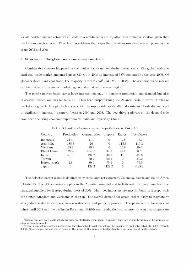
Considerable changes happened in the market for steam coal during recent years. The global seaborne
hard coal trade market amounted up to 839 Mt in 2008 an increase of 58% compared to the year 2000. Of
global seaborn hard coal trade, the majority is steam coal1 (639 Mt in 2008). The seaborne trade market
can be divided into a pacific market region and an atlantic market region2.
The pacific market basin saw a large increase not only in domestic production and demand but also
in seaward traded volumes (cf table 1). It has been outperforming the Atlantic basin in terms of relative
market size growth through the last years. On the supply side, especially Indonesia and Australia managed
to significantly increase its exports between 2000 and 2008. The new driving players on the demand side
have been the rising economic superpowers: India and especially China .
Table 1: Selected data for steam coal for the pacific basin for 2008 in Mt
Country Production Consumption Import Export Net-Export
Indonesia 214.9 41.9 0 173 173Australia 185.3 70 0 115.3 115.3Vietnam 39.9 19.9 0 20.6 20.6PR of China 2334 2340.1 34.2 42.7 8.5India 461.9 491.7 30.9 1.1 -29.8Taiwan 0 60.2 60.2 0 -60.2Korea. south 2.8 80.9 75.5 0 -75.5Japan 0 128.2 128.2 0 -128.2
The Atlantic market region is dominated by three large net exporters, Colombia, Russia and South Africa
(cf table 2). The US is a swing supplier in the Atlantic basin and mid to high cost US mines have been the
marginal suppliers for Europe during most of 2008. Main net importers are mostly found in Europe with
the United Kingdom and Germany at the top. The overall demand for steam coal is likely to stagnate or
slowly decline due to carbon emission restrictions and public opposition. The phase out of German coal
mines until 2018 and the decline in Polish and British coal production will counter or even overcompensate
1Steam coal are hard coals which are used in electricity geenration. Typically, they are of sub-bituminous, bituminous oreven anthracite quality.
2From a market integration perspective the steam trade coal market can be considered well integrated (Li, 2008; Warell,2006). Nevertheless, we use this division in the scope of this paper to better structure our analysis of market actors.
4
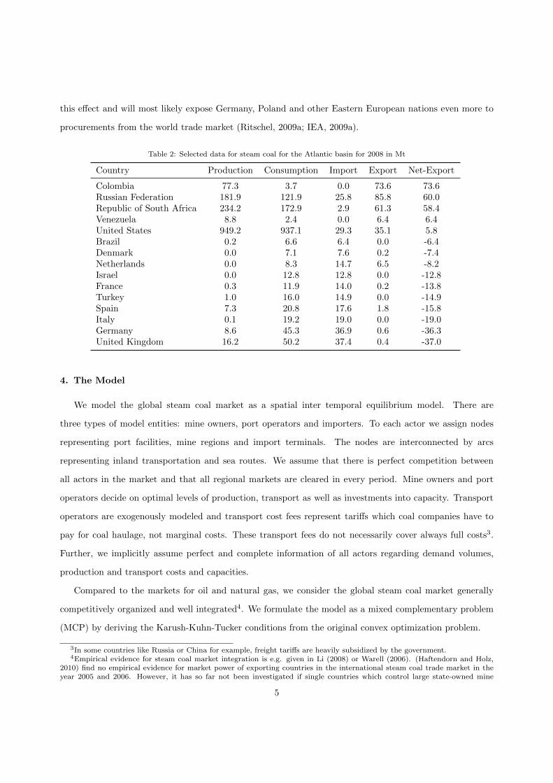
this effect and will most likely expose Germany, Poland and other Eastern European nations even more to
procurements from the world trade market (Ritschel, 2009a; IEA, 2009a).
Table 2: Selected data for steam coal for the Atlantic basin for 2008 in Mt
Country Production Consumption Import Export Net-Export
Colombia 77.3 3.7 0.0 73.6 73.6Russian Federation 181.9 121.9 25.8 85.8 60.0Republic of South Africa 234.2 172.9 2.9 61.3 58.4Venezuela 8.8 2.4 0.0 6.4 6.4United States 949.2 937.1 29.3 35.1 5.8Brazil 0.2 6.6 6.4 0.0 -6.4Denmark 0.0 7.1 7.6 0.2 -7.4Netherlands 0.0 8.3 14.7 6.5 -8.2Israel 0.0 12.8 12.8 0.0 -12.8France 0.3 11.9 14.0 0.2 -13.8Turkey 1.0 16.0 14.9 0.0 -14.9Spain 7.3 20.8 17.6 1.8 -15.8Italy 0.1 19.2 19.0 0.0 -19.0Germany 8.6 45.3 36.9 0.6 -36.3United Kingdom 16.2 50.2 37.4 0.4 -37.0
4. The Model
We model the global steam coal market as a spatial inter temporal equilibrium model. There are
three types of model entities: mine owners, port operators and importers. To each actor we assign nodes
representing port facilities, mine regions and import terminals. The nodes are interconnected by arcs
representing inland transportation and sea routes. We assume that there is perfect competition between
all actors in the market and that all regional markets are cleared in every period. Mine owners and port
operators decide on optimal levels of production, transport as well as investments into capacity. Transport
operators are exogenously modeled and transport cost fees represent tariffs which coal companies have to
pay for coal haulage, not marginal costs. These transport fees do not necessarily cover always full costs3.
Further, we implicitly assume perfect and complete information of all actors regarding demand volumes,
production and transport costs and capacities.
Compared to the markets for oil and natural gas, we consider the global steam coal market generally
competitively organized and well integrated4. We formulate the model as a mixed complementary problem
(MCP) by deriving the Karush-Kuhn-Tucker conditions from the original convex optimization problem.
3In some countries like Russia or China for example, freight tariffs are heavily subsidized by the government.4Empirical evidence for steam coal market integration is e.g. given in Li (2008) or Warell (2006). (Haftendorn and Holz,
2010) find no empirical evidence for market power of exporting countries in the international steam coal trade market in theyear 2005 and 2006. However, it has so far not been investigated if single countries which control large state-owned mine
5
4.1. Notation
In this section we provide a description of the sets, parameters and variables used in the model formula-
tion. The time horizon of the model T = 2005, 2006, . . . , t, . . . , 2030 includes periods on an annual basis
from 2005 until 2015, and time periods in five step intervals from 2015 onwards to 2030. The model consists
of a network NW (N,A), where N is a set of nodes and A is a set of arcs between the nodes. The set of
nodes N can be divided into three subsets N ≡ P ∪M ∪ I, where m ∈ M is a mining region, p ∈ P is
a export terminal and i ∈ I is a demand node. The three different roles of nodes are mutually exclusive
P ∩M ≡ P ∩ I ≡ I ∩M ≡ ∅. The set of arcs A ⊆ N × N consists of arcs a(i,j) where (i, j) is a tuple of
nodes i, j ∈ N .
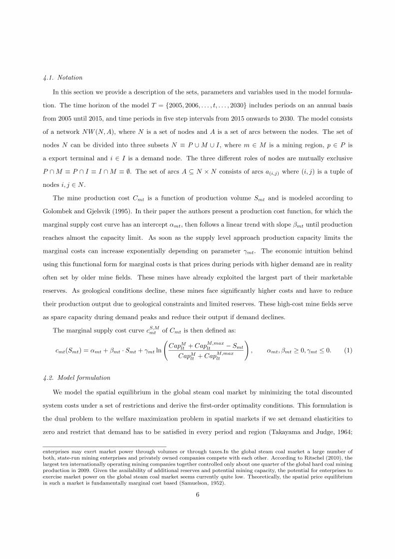
The mine production cost Cmt is a function of production volume Smt and is modeled according to
Golombek and Gjelsvik (1995). In their paper the authors present a production cost function, for which the
marginal supply cost curve has an intercept αmt, then follows a linear trend with slope βmt until production
reaches almost the capacity limit. As soon as the supply level approach production capacity limits the
marginal costs can increase exponentially depending on parameter γmt. The economic intuition behind
using this functional form for marginal costs is that prices during periods with higher demand are in reality
often set by older mine fields. These mines have already exploited the largest part of their marketable
reserves. As geological conditions decline, these mines face significantly higher costs and have to reduce
their production output due to geological constraints and limited reserves. These high-cost mine fields serve
as spare capacity during demand peaks and reduce their output if demand declines.
The marginal supply cost curve cS,Mmt of Cmt is then defined as:
cmt(Smt) = αmt + βmt · Smt + γmt ln
(CapMlt + CapM,max
lt − Smt
CapMlt + CapM,maxlt
), αmt, βmt ≥ 0, γmt ≤ 0. (1)
4.2. Model formulation
We model the spatial equilibrium in the global steam coal market by minimizing the total discounted
system costs under a set of restrictions and derive the first-order optimality conditions. This formulation is
the dual problem to the welfare maximization problem in spatial markets if we set demand elasticities to
zero and restrict that demand has to be satisfied in every period and region (Takayama and Judge, 1964;
enterprises may exert market power through volumes or through taxes.In the global steam coal market a large number ofboth, state-run mining enterprises and privately owned companies compete with each other. According to Ritschel (2010), thelargest ten internationally operating mining companies together controlled only about one quarter of the global hard coal miningproduction in 2009. Given the availability of additional reserves and potential mining capacity, the potential for enterprises toexercise market power on the global steam coal market seems currently quite low. Theoretically, the spatial price equilibriumin such a market is fundamentally marginal cost based (Samuelson, 1952).
6
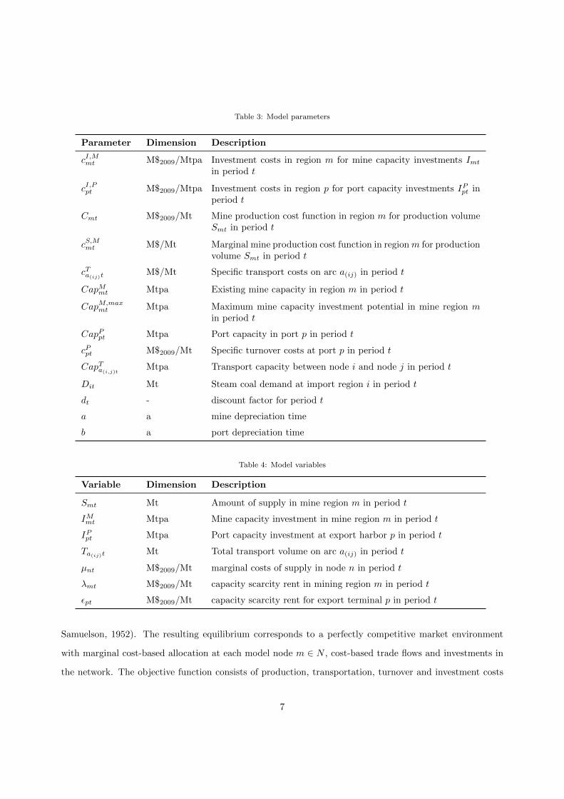
Table 3: Model parameters
Parameter Dimension Description
cI,Mmt M$2009/Mtpa Investment costs in region m for mine capacity investments Imt
in period t
cI,Ppt M$2009/Mtpa Investment costs in region p for port capacity investments IPpt inperiod t
Cmt M$2009/Mt Mine production cost function in region m for production volumeSmt in period t
cS,Mmt M$/Mt Marginal mine production cost function in regionm for productionvolume Smt in period t
cTa(ij)tM$/Mt Specific transport costs on arc a(ij) in period t
CapMmt Mtpa Existing mine capacity in region m in period t
CapM,maxmt Mtpa Maximum mine capacity investment potential in mine region m
in period t
CapPpt Mtpa Port capacity in port p in period t
cPpt M$2009/Mt Specific turnover costs at port p in period t
CapTa(i,j)tMtpa Transport capacity between node i and node j in period t
Dit Mt Steam coal demand at import region i in period t
dt - discount factor for period t
a a mine depreciation time
b a port depreciation time
Table 4: Model variables
Variable Dimension Description
Smt Mt Amount of supply in mine region m in period t
IMmt Mtpa Mine capacity investment in mine region m in period t
IPpt Mtpa Port capacity investment at export harbor p in period t
Ta(ij)t Mt Total transport volume on arc a(ij) in period t
µnt M$2009/Mt marginal costs of supply in node n in period t
λmt M$2009/Mt capacity scarcity rent in mining region m in period t
εpt M$2009/Mt capacity scarcity rent for export terminal p in period t
Samuelson, 1952). The resulting equilibrium corresponds to a perfectly competitive market environment
with marginal cost-based allocation at each model node m ∈ N , cost-based trade flows and investments in
the network. The objective function consists of production, transportation, turnover and investment costs
7
that every producer and port operator minimizes with respect to satisfaction of demand. Producers sell
their coal at the export terminals to exporters and traders who ship the coal via bulk carriers on a least cost
basis to the demand centers. Turnover costs are interpreted as marginal costs. Costs for transport represent
prices and tariffs which are relevant for coal producers and exporters. Note that these transport tariffs not
necessarily have to coincide with full costs. In many countries, e.g. Russia and China, transportation tariffs
are set by regulatory institutions and are often subsidized. With keeping our mentioned assumptions in
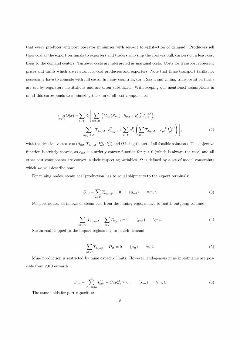
mind this corresponds to minimizing the sum of all cost components:
minx∈Ω
O(x) =∑t∈T
dt
[ ∑m∈M
(Cmt(Smt) · Smt + cI,Mmt I
I,Mmt
)+
∑a(ij)∈A
Ta(ij)t · cTa(ij)t
+∑p∈P
cPpt
(∑i∈I
Ta(pi)t + cI,Ppt II,Ppt
)], (2)
with the decision vector x = (Smt, Ta(ij)t, IMmt, I
Ppt) and Ω being the set of all feasible solutions. The objective
function is strictly convex, as cmt is a strictly convex function for γ < 0 (which is always the case) and all
other cost components are convex in their respecting variables. Ω is defined by a set of model constraints
which we will describe now:
For mining nodes, steam coal production has to equal shipments to the export terminals:
Smt −∑p∈P
Ta(mp)t = 0 (µmt) ∀m, t. (3)
For port nodes, all inflows of steam coal from the mining regions have to match outgoing volumes:
∑m∈M
Ta(mp)t −∑i∈I
Ta(pi)t = 0 (µpt) ∀p, t. (4)
Steam coal shipped to the import regions has to match demand:
∑p∈P
Ta(pi)t −Dit = 0 (µit) ∀i, t. (5)
Mine production is restricted by mine capacity limits. However, endogenous mine investments are pos-
sible from 2010 onwards:
Smt −t∑
t′=2010
IMmt′ − CapMmt ≤ 0, (λmt) ∀m, t. (6)
The same holds for port capacities:
8
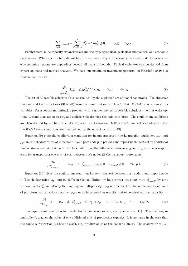
∑i∈I
Ta(pi)t −t∑
t′=2010
IPpt′ − CapPpt ≤ 0, (φpt) ∀p, t. (7)
Furthermore, mine capacity expansions are limited by geographical, geological and political and economic
parameters. While such potentials are hard to estimate, they are necessary to avoid that the most cost
efficient mine regions are expanding beyond all realistic bounds. Typical estimates can be derived from
expert opinions and market analyses. We base our maximum investment potential on Ritschel (2009b) so
that we can restrict:
t∑t′=2010
IMmt′ − CapM,maxmt ≤ 0, (εmt) ∀m, t. (8)
The set of all feasible solutions Ω is constrained by the explained set of model constrains. The objective
function and the restrictions (3) to (8) form our minimization problem WCM . WCM is convex in all its
variables. For a convex minimization problem with a non-empty set of feasible solutions, the first order op-
timality conditions are necessary and sufficient for deriving the unique solution. The equilibrium conditions
are then derived by the first order derivatives of the Lagrangian L (Karush-Kuhn-Tucker conditions). For
the WCM these conditions are then defined by the equations (9) to (13).
Equation (9) gives the equilibrium condition for inland transport. the Lagrangian multipliers µmt and
µpt are the shadow prices at mine node m and port node p in period t and represent the costs of an additional
unit of steam coal at that node. In the equilibrium, the difference between µmt and µpt are the transport
costs for transporting one unit of coal between both nodes (if the transport route exists)
∂L
∂Ta(mp)t: µmt + dt · cTa(mp)t
− µpt ≥ 0 ⊥ Ta(mp)t ≥ 0 ∀m, p, t. (9)
Equation (10) gives the equilibrium condition for sea transport between port node p and import node
i. The shadow prices µpt and µit differ in the equilibrium by bulk carrier transport rates cTa(mp)t, by port
turnover costs cPpt and also by the Lagrangian multiplier φpt. φpt represents the value of one additional unit
of port turnover capacity at port p. φpt can be interpreted as scarcity rent of constrained port capacity
∂L
∂Ta(pi)t: µpt + dt · cTa(mp)t
+ dt · cPpt + φpt − µit ≥ 0 ⊥ Ta(pi)t ≥ 0 ∀p, i, t. (10)
The equilibrium condition for production at mine nodes is given by equation (11). The Lagrangian
multiplier λmt gives the value of one additional unit of production capacity. It is non-zero in the case that
the capacity restriction (3) has no slack, e.g. production is at the capacity limits. The shadow price µmt
9
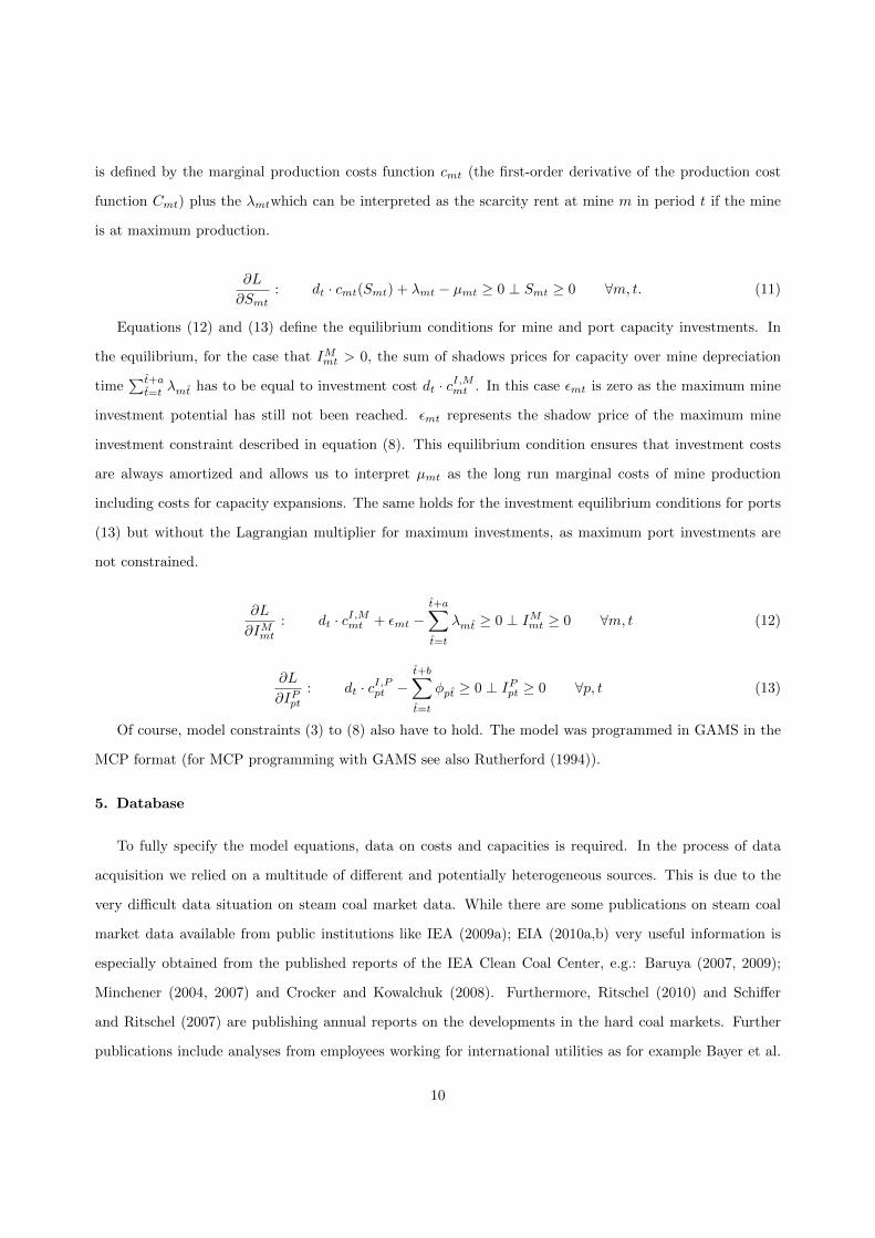
is defined by the marginal production costs function cmt (the first-order derivative of the production cost
function Cmt) plus the λmtwhich can be interpreted as the scarcity rent at mine m in period t if the mine
is at maximum production.
∂L
∂Smt: dt · cmt(Smt) + λmt − µmt ≥ 0 ⊥ Smt ≥ 0 ∀m, t. (11)
Equations (12) and (13) define the equilibrium conditions for mine and port capacity investments. In
the equilibrium, for the case that IMmt > 0, the sum of shadows prices for capacity over mine depreciation
time∑t+a
t=tλmt has to be equal to investment cost dt · cI,Mmt . In this case εmt is zero as the maximum mine
investment potential has still not been reached. εmt represents the shadow price of the maximum mine
investment constraint described in equation (8). This equilibrium condition ensures that investment costs
are always amortized and allows us to interpret µmt as the long run marginal costs of mine production
including costs for capacity expansions. The same holds for the investment equilibrium conditions for ports
(13) but without the Lagrangian multiplier for maximum investments, as maximum port investments are
not constrained.
∂L
∂IMmt
: dt · cI,Mmt + εmt −t+a∑t=t
λmt ≥ 0 ⊥ IMmt ≥ 0 ∀m, t (12)
∂L
∂IPpt: dt · cI,Ppt −
t+b∑t=t
φpt ≥ 0 ⊥ IPpt ≥ 0 ∀p, t (13)
Of course, model constraints (3) to (8) also have to hold. The model was programmed in GAMS in the
MCP format (for MCP programming with GAMS see also Rutherford (1994)).
5. Database
To fully specify the model equations, data on costs and capacities is required. In the process of data
acquisition we relied on a multitude of different and potentially heterogeneous sources. This is due to the
very difficult data situation on steam coal market data. While there are some publications on steam coal
market data available from public institutions like IEA (2009a); EIA (2010a,b) very useful information is
especially obtained from the published reports of the IEA Clean Coal Center, e.g.: Baruya (2007, 2009);
Minchener (2004, 2007) and Crocker and Kowalchuk (2008). Furthermore, Ritschel (2010) and Schiffer
and Ritschel (2007) are publishing annual reports on the developments in the hard coal markets. Further
publications include analyses from employees working for international utilities as for example Bayer et al.
10
(2009) and Kopal (2008). Industry yearbooks can provide useful information as it is the case for China (PRC,
2007, 2006). National statistics bureaus and mineral ministries seem to provide high quality information,
but reports on hard coal mining industries are at best scarce, with notable exceptions of ABARE (2008)
and ABS (2006). Not mentioned are a larger number of coal company annual reports as well as information
based on expert interviews. Furthermore, our analysis is based on several extensive research projects of
Trueby (2009) and Eichmueller (2010) at the Institute of Energy Economics at the University of Cologne.
To account for the varying steam coal qualities worldwide, the WCM converts mass units fed into the
model into energy flows. All model outputs are therefore given in standardized energy-mass units with one
tonne equaling 25120,8 MJ (or 6000 kcal per kg). Information on average energy content is based on Ritschel
(2009a); IEA (2009a) and BGR (2008).
5.1. Topology
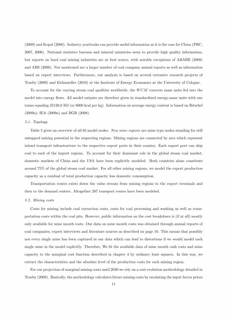
Table 5 gives an overview of all 65 model nodes. New mine regions are mine type nodes standing for still
untapped mining potential in the respecting regions. Mining regions are connected by arcs which represent
inland transport infrastructure to the respective export ports in their country. Each export port can ship
coal to each of the import regions. To account for their dominant role in the global steam coal market,
domestic markets of China and the USA have been explicitly modeled. Both countries alone constitute
around 75% of the global steam coal market. For all other mining regions, we model the export production
capacity as a residual of total production capacity less domestic consumption.
Transportation routes exists down the value stream from mining regions to the export terminals and
then to the demand centers. Altogether 287 transport routes have been modeled.
5.2. Mining costs
Costs for mining include coal extraction costs, costs for coal processing and washing as well as trans-
portation costs within the coal pits. However, public information on the cost breakdown is (if at all) mostly
only available for mine mouth costs. Our data on mine mouth costs was obtained through annual reports of
coal companies, expert interviews and literature sources as described on page 10. This means that possibly
not every single mine has been captured in our data which can lead to distortions if we would model each
single mine in the model explicitly. Therefore, We fit the available data of mine mouth cash costs and mine
capacity to the marginal cost function described in chapter 4 by ordinary least squares. In this way, we
extract the characteristics and the absolute level of the production costs for each mining region.
For our projection of marginal mining costs until 2030 we rely on a cost evolution methodology detailed in
Trueby (2009). Basically, the methodology calculates future mining costs by escalating the input factor prices
11
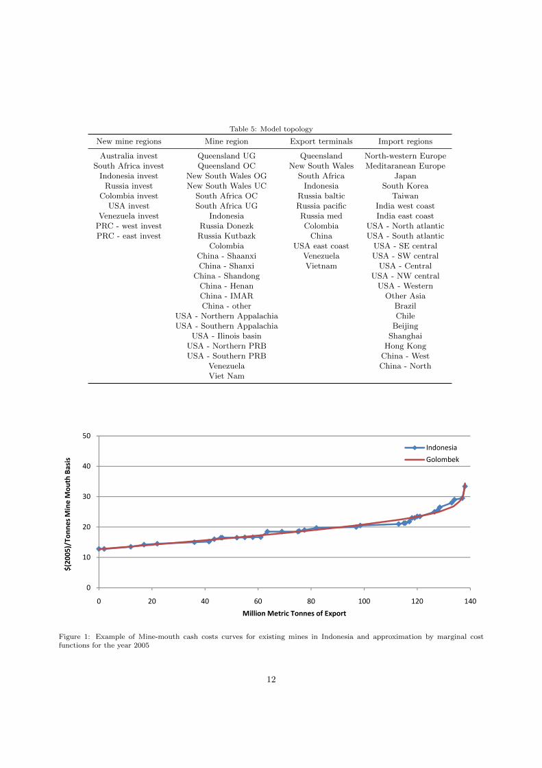
Table 5: Model topology
New mine regions Mine region Export terminals Import regions
Australia invest Queensland UG Queensland North-western EuropeSouth Africa invest Queensland OC New South Wales Meditaranean Europe
Indonesia invest New South Wales OG South Africa JapanRussia invest New South Wales UC Indonesia South Korea
Colombia invest South Africa OC Russia baltic TaiwanUSA invest South Africa UG Russia pacific India west coast
Venezuela invest Indonesia Russia med India east coastPRC - west invest Russia Donezk Colombia USA - North atlanticPRC - east invest Russia Kutbazk China USA - South atlantic
Colombia USA east coast USA - SE centralChina - Shaanxi Venezuela USA - SW centralChina - Shanxi Vietnam USA - Central
China - Shandong USA - NW centralChina - Henan USA - WesternChina - IMAR Other AsiaChina - other Brazil
USA - Northern Appalachia ChileUSA - Southern Appalachia Beijing
USA - Ilinois basin ShanghaiUSA - Northern PRB Hong KongUSA - Southern PRB China - West
Venezuela China - NorthViet Nam
20
30
40
50
/Ton
nes M
ine
Mou
th B
asis
Indonesia
Golombek
0
10
20
30
40
50
0 20 40 60 80 100 120 140
$(20
05)/
Tonn
es M
ine
Mou
th B
asis
Million Metric Tonnes of Export
Indonesia
Golombek
Figure 1: Example of Mine-mouth cash costs curves for existing mines in Indonesia and approximation by marginal costfunctions for the year 2005
12
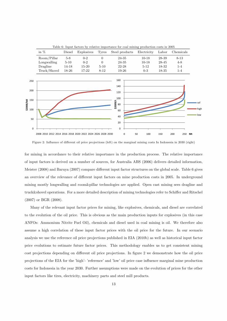
Table 6: Input factors by relative importance for coal mining production costs in 2005
in % Diesel Explosives Tyres Steel products Electricity Labor Chemicals
Room/Pillar 5-8 0-2 0 24-35 10-18 28-39 8-13Longwalling 5-10 0-2 0 24-35 10-18 28-45 4-8Dragline 14-18 15-20 5-10 22-28 5-12 18-32 1-4Truck/Shovel 18-26 17-22 8-12 19-26 0-3 18-35 1-4
250
200
250
150
200
250
8/bb
l
100
150
200
250
$200
8/bb
l
50
100
150
200
250
$200
8/bb
l
0
50
100
150
200
250
$200
8/bb
l
0
50
100
150
200
250
2008 2010 2012 2014 2016 2018 2020 2022 2024 2026 2028 2030
$200
8/bb
l
0
50
100
150
200
250
2008 2010 2012 2014 2016 2018 2020 2022 2024 2026 2028 2030
$200
8/bb
l
140
160
120
140
160
80
100
120
140
160
09/t ref
60
80
100
120
140
160
$200
9/t
ref
high
l
20
40
60
80
100
120
140
160
$200
9/t
ref
high
low
0
20
40
60
80
100
120
140
160
$200
9/t
ref
high
low
0
20
40
60
80
100
120
140
160
0 50 100 150 200 250
$200
9/t
Mt
ref
high
low
0
20
40
60
80
100
120
140
160
0 50 100 150 200 250
$200
9/t
Mt
ref
high
low
Figure 2: Influence of different oil price projections (left) on the marginal mining costs In Indonesia in 2030 (right)
for mining in accordance to their relative importance in the production process. The relative importance
of input factors is derived on a number of sources, for Australia ABS (2006) delivers detailed information,
Meister (2008) and Baruya (2007) compare different input factor structures on the global scale. Table 6 gives
an overview of the relevance of different input factors on mine production costs in 2005. In underground
mining mostly longwalling and room&pillar technologies are applied. Open cast mining sees dragline and
truck&shovel operations. For a more detailed description of mining technologies refer to Schiffer and Ritschel
(2007) or BGR (2008).
Many of the relevant input factor prices for mining, like explosives, chemicals, and diesel are correlated
to the evolution of the oil price. This is obvious as the main production inputs for explosives (in this case
ANFOs: Ammonium Nitrite Fuel Oil), chemicals and diesel used in coal mining is oil. We therefore also
assume a high correlation of these input factor prices with the oil price for the future. In our scenario
analysis we use the reference oil price projections published in EIA (2010b) as well as historical input factor
price evolutions to estimate future factor prices. This methodology enables us to get consistent mining
cost projections depending on different oil price projections. In figure 2 we demonstrate how the oil price
projections of the EIA for the ’high’- ’reference’ and ’low’ oil price case influence marginal mine production
costs for Indonesia in the year 2030. Further assumptions were made on the evolution of prices for the other
input factors like tires, electricity, machinery parts and steel mill products.
13
5.3. Costs for transport, turnover and investments
Inland transportation costs depend strongly on the vehicles used. The three most important transport
modes are railway, trucks and river barges in descending order. Selection of transport modes depends greatly
on local conditions: Indonesia for example utilizes its network of navigable rivers on Kalimantan to transport
most of its coal production with river barges to the export terminals. In countries like China, Australia or
Russia, railways carry the bulk of the coal transport. Information on transportation modes and costs of
domestic transport is based on Minchener (2004, 2007); Ritschel (2010) and Eichmueller (2010).
To get estimates for the evolution of future domestic transportation costs we follow a similar methodology
as done for mining production costs. We inflate inland transportation costs with the estimated impact of
diesel and electricity prices on inland transportation per country. We estimated the relative impact of diesel
and electricity by the relative importance of truck haulage and railway haulage for the main transport routes.
Truck haulage and barge haulage would mean a complete dependence on diesel prices while railway haulage
would mean at least a mix between diesel and electricity.
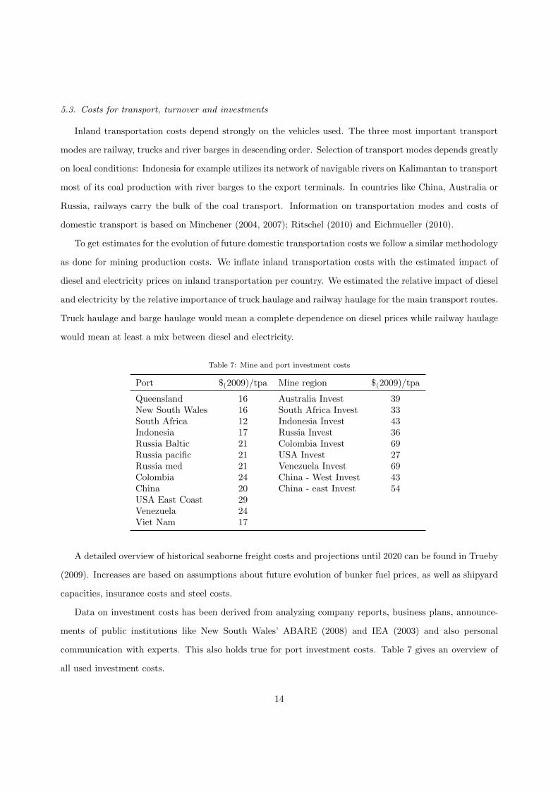
Table 7: Mine and port investment costs
Port $(2009)/tpa Mine region $(2009)/tpa
Queensland 16 Australia Invest 39New South Wales 16 South Africa Invest 33South Africa 12 Indonesia Invest 43Indonesia 17 Russia Invest 36Russia Baltic 21 Colombia Invest 69Russia pacific 21 USA Invest 27Russia med 21 Venezuela Invest 69Colombia 24 China - West Invest 43China 20 China - east Invest 54USA East Coast 29Venezuela 24Viet Nam 17
A detailed overview of historical seaborne freight costs and projections until 2020 can be found in Trueby
(2009). Increases are based on assumptions about future evolution of bunker fuel prices, as well as shipyard
capacities, insurance costs and steel costs.
Data on investment costs has been derived from analyzing company reports, business plans, announce-
ments of public institutions like New South Wales’ ABARE (2008) and IEA (2003) and also personal
communication with experts. This also holds true for port investment costs. Table 7 gives an overview of
all used investment costs.
14
’
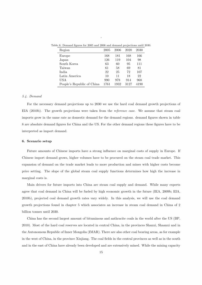
Table 8: Demand figures for 2005 and 2006 and demand projections until 2030.
Region 2005 2006 2020 2030
Europe 168 181 168 166Japan 126 119 104 98South Korea 63 60 95 111Taiwan 61 58 69 81India 22 25 72 107Latin America 10 11 18 22USA 990 978 914 968People’s Republic of China 1761 1932 3127 4190
5.4. Demand
For the necessary demand projections up to 2030 we use the hard coal demand growth projections of
EIA (2010b). The growth projections were taken from the reference case. We assume that steam coal
imports grow in the same rate as domestic demand for the demand regions. demand figures shown in table
8 are absolute demand figures for China and the US. For the other demand regions these figures have to be
interpreted as import demand.
6. Scenario setup
Future amounts of Chinese imports have a strong influence on marginal costs of supply in Europe. If
Chinese import demand grows, higher volumes have to be procured on the steam coal trade market. This
expansion of demand on the trade market leads to more production and mines with higher costs become
price setting. The slope of the global steam coal supply functions determines how high the increase in
marginal costs is.
Main drivers for future imports into China are steam coal supply and demand. While many experts
agree that coal demand in China will be fueled by high economic growth in the future (IEA, 2009b; EIA,
2010b), projected coal demand growth rates vary widely. In this analysis, we will use the coal demand
growth projections found in chapter 5 which associates an increase in steam coal demand in China of 2
billion tonnes until 2030.
China has the second largest amount of bituminous and anthracite coals in the world after the US (BP,
2010). Most of the hard coal reserves are located in central China, in the provinces Shanxi, Shaanxi and in
the Autonomous Republic of Inner Mongolia (IMAR). There are also other coal bearing areas, as for example
in the west of China, in the province Xinjiang. The coal fields in the central provinces as well as in the south
and in the east of China have already been developed and are extensively mined. While the mining capacity
15
limits can still be further extended, most of the mines are already operating deep underground at elevated
cost levels. As Dorian (2005) and Taoa and Li (2007) state, future prospects could lie in the desert province
Xinjiang, where coal reserves are plentiful and could still be mined in cost-efficient open cast operations.
One important hindrance why these lucrative reserves have not been developed so far is the lack of
large scale transport infrastructure between the demand hubs on the coast and the eastern regions. Coal
transport in China mainly takes place by railway, river barges and coastal shipping. So far, mine-mouth
coal-fired power plants in combination with large scale HVDC lines which transport electricity to the coastal
demand centers are scarce but are increasingly in the focus of Chinese grid planning authorities (Yinbiao,
2004; Qingyun, 2005).
The projected massive growth in steam coal demand of 2 billion tonnes until 2030 will have to be trans-
ported from the main production regions in the center and in the west of China to the coastal demand hubs.
In our analysis, we will investigate two scenarios with different assumptions on the transport investments
taking place in China to deliver coal-based energy to the demand hubs.
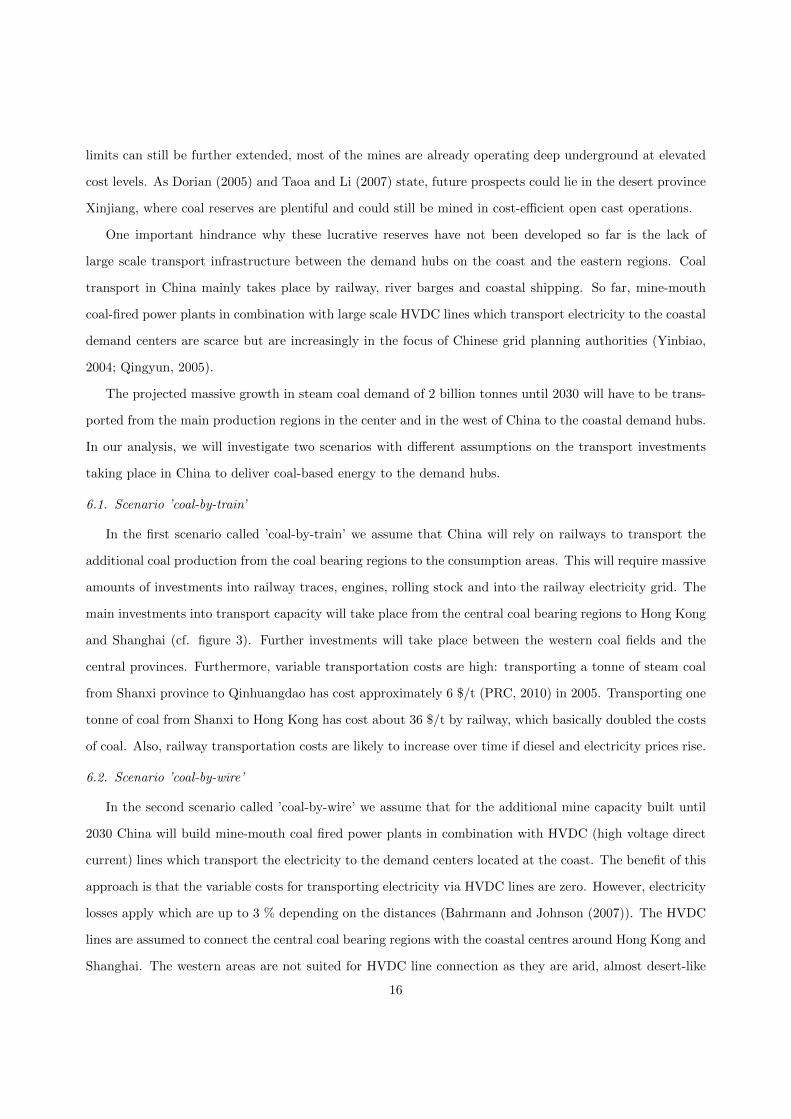
6.1. Scenario ’coal-by-train’
In the first scenario called ’coal-by-train’ we assume that China will rely on railways to transport the
additional coal production from the coal bearing regions to the consumption areas. This will require massive
amounts of investments into railway traces, engines, rolling stock and into the railway electricity grid. The
main investments into transport capacity will take place from the central coal bearing regions to Hong Kong
and Shanghai (cf. figure 3). Further investments will take place between the western coal fields and the
central provinces. Furthermore, variable transportation costs are high: transporting a tonne of steam coal
from Shanxi province to Qinhuangdao has cost approximately 6 $/t (PRC, 2010) in 2005. Transporting one
tonne of coal from Shanxi to Hong Kong has cost about 36 $/t by railway, which basically doubled the costs
of coal. Also, railway transportation costs are likely to increase over time if diesel and electricity prices rise.
6.2. Scenario ’coal-by-wire’
In the second scenario called ’coal-by-wire’ we assume that for the additional mine capacity built until
2030 China will build mine-mouth coal fired power plants in combination with HVDC (high voltage direct
current) lines which transport the electricity to the demand centers located at the coast. The benefit of this
approach is that the variable costs for transporting electricity via HVDC lines are zero. However, electricity
losses apply which are up to 3 % depending on the distances (Bahrmann and Johnson (2007)). The HVDC
lines are assumed to connect the central coal bearing regions with the coastal centres around Hong Kong and
Shanghai. The western areas are not suited for HVDC line connection as they are arid, almost desert-like
16
Chinese import volumes are heavily influenced by inland transportation costs and capacities
Coal-by-wire 2030 Coal-by-train 2030
- 6 -
Demand Hub
Supply regions
HVDC lines
Railway transport
Figure 3: Topology of the scenario setup for China
regions. Therefore, it is unlikely that enough water for the cooling circuits of large-scale coal fired generation
capacity will be available there. Coal from western provinces will be transported via railway to the central
coal bearing areas where they will fuel coal-fired electricity generation in combination with HVDC lines to
the demand centers. As we only model the coal market, all numbers on coal flows from the mining regions
China - west invest and China - east invest to the demand regions have to be understood as electricity
equivalents, as the respective coal flows are burnt in mine-mouth coal-fired power plants which transport
the generated electricity via HVDC lines to the demand hubs.
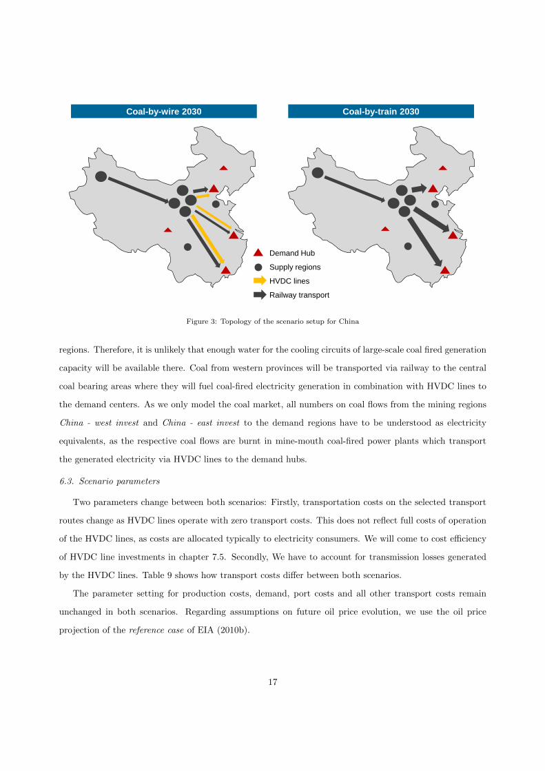
6.3. Scenario parameters
Two parameters change between both scenarios: Firstly, transportation costs on the selected transport
routes change as HVDC lines operate with zero transport costs. This does not reflect full costs of operation
of the HVDC lines, as costs are allocated typically to electricity consumers. We will come to cost efficiency
of HVDC line investments in chapter 7.5. Secondly, We have to account for transmission losses generated
by the HVDC lines. Table 9 shows how transport costs differ between both scenarios.
The parameter setting for production costs, demand, port costs and all other transport costs remain
unchanged in both scenarios. Regarding assumptions on future oil price evolution, we use the oil price
projection of the reference case of EIA (2010b).
17
Table 9: Parameter settings for domestic steam coal transport costs in both scenarios
2005 2030
in $2009/t coal-by-wire coal-by-train coal-by-wire coal-by-train
costs from Shanxi to:Hong Kong 26 26 0 44
Shanghai 36 36 0 61Beijing 6 6 0 11
costs from Shaanxi to:Hong Kong 31 31 0 60
Shanghai 23 23 0 44Beijing 18 18 0 36
costs from IMAR to:Hong Kong 43 43 0 69
Shanghai 31 31 0 51Beijing 11 11 0 18
costs from Xinjiang to:Hong Kong 65 65 49 99
Shanghai 60 60 49 90Beijing 57 57 49 86
7. Results
In this chapter we will outline main model results for the two analyzed scenarios ’coal-by-train’ and
’coal-by-wire’. We will validate the model for the base years 2005 and 2006 and then depict marginal costs,
trade flows, utilization and welfare effects in the scenario runs for 2020 and 2030.
7.1. Coal Supply in China
Table 10 shows how Chinese coal demand is covered in both scenarios until the model year 2030. The
results for the years 2005 and 2006 show, that the model is fairly accurately calibrated an can reproduce the
historic production mix. However, reference figures are production volumes and therefore it is not possible
to validate domestic trade flows between different Chinese regions.
In the ’coal-by-train’ scenario, the main coal suppliers are the central Chinese provinces Shanxi, Shaanxi
and IMAR in 2030. They supply 2050 Mt via land transport (mostly railway). A further part of their
production is transported to the norther export terminals of Qinhuangdao and shipped via handy size bulk
vessels or coastal barges to the Shanghai and Hong Kong regions. This is depicted in table 10 in the
category ’reimports’. Western coalfields supply roughly 350 Mt of steam coal via land transports in 2030.
The production in the rest of China amounts to approximately 936 Mt and is therefore slightly above todays
levels.
Most importantly, imports play a significant role in the ’coal-by-train’ scenario, amounting up to 277 Mt.
While this seems to be a fairly small volume compared to overall Chinese demand of more than 4 billion
18
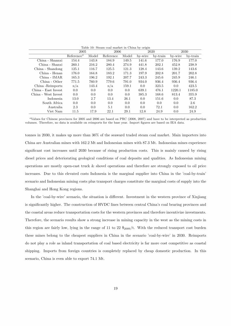
Table 10: Steam coal market in China by origin
2005 2006 2020 2030
Referencea Model Reference Model by-wire by-train by-wire by-train
China - Shaanxi 154.4 143.8 184.9 149.5 141.6 177.0 176.9 177.0China - Shanxi 260.1 216.2 280.4 274.9 441.8 202.1 452.8 238.9
China - Shandong 125.1 116.7 125.5 121.3 128.4 143.6 139.2 143.6China - Henan 176.0 164.8 183.2 171.3 197.9 202.8 201.7 202.8China - IMAR 165.3 196.2 192.1 207.7 243.3 245.6 245.9 246.1China - Other 771.5 760.9 779.6 791.0 934.0 936.4 936.4 936.4
China -Reimports n/a 143.4 n/a 159.1 0.0 323.5 0.0 423.5China - East Invest 0.0 0.0 0.0 0.0 639.1 476.1 1220.1 1185.0China - West Invest 0.0 0.0 0.0 0.0 385.3 168.6 813.4 355.9
Indonesia 13.0 2.7 13.4 26.1 0.0 151.6 0.0 87.3South Africa 0.0 0.0 0.0 0.0 0.0 0.0 0.0 2.6
Australia 2.3 0.0 5.1 0.0 0.0 72.1 0.0 162.2Viet Nam 11.5 17.9 22.1 29.1 12.8 24.9 0.0 24.9
aValues for Chinese provinces for 2005 and 2006 are based on PRC (2008, 2007) and have to be interpreted as productionvolumes. Therefore, no data is available on reimports for the base year. Import figures are based on IEA data.
tonnes in 2030, it makes up more than 36% of the seaward traded steam coal market. Main importers into
China are Australian mines with 162.2 Mt and Indonesian mines with 87.3 Mt. Indonesian mines experience
significant cost increases until 2030 because of rising production costs. This is mainly caused by rising
diesel prices and deteriorating geological conditions of coal deposits and qualities. As Indonesian mining
operations are mostly open-cast truck & shovel operations and therefore are strongly exposed to oil price
increases. Due to this elevated costs Indonesia is the marginal supplier into China in the ’coal-by-train’
scenario and Indonesian mining costs plus transport charges constitute the marginal costs of supply into the
Shanghai and Hong Kong regions.
In the ’coal-by-wire’ scenario, the situation is different. Investment in the western province of Xinjiang
is significantly higher. The construction of HVDC lines between central China’s coal bearing provinces and
the coastal areas reduce transportation costs for the western provinces and therefore incentivize investments.
Therefore, the scenario results show a strong increase in mining capacity in the west as the mining costs in
this region are fairly low, lying in the range of 11 to 22 $2009/t. With the reduced transport cost burden
these mines belong to the cheapest suppliers in China in the scenario ’coal-by-wire’ in 2030. Reimports
do not play a role as inland transportation of coal based electricity is far more cost competitive as coastal
shipping. Imports from foreign countries is completely replaced by cheap domestic production. In this
scenario, China is even able to export 74.1 Mt.
19
7.2. Coal Supply in Europe
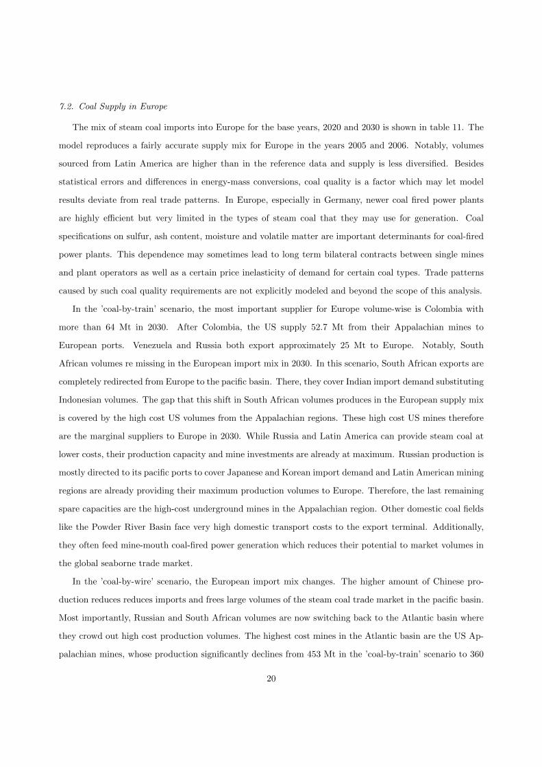
The mix of steam coal imports into Europe for the base years, 2020 and 2030 is shown in table 11. The
model reproduces a fairly accurate supply mix for Europe in the years 2005 and 2006. Notably, volumes
sourced from Latin America are higher than in the reference data and supply is less diversified. Besides
statistical errors and differences in energy-mass conversions, coal quality is a factor which may let model
results deviate from real trade patterns. In Europe, especially in Germany, newer coal fired power plants
are highly efficient but very limited in the types of steam coal that they may use for generation. Coal
specifications on sulfur, ash content, moisture and volatile matter are important determinants for coal-fired
power plants. This dependence may sometimes lead to long term bilateral contracts between single mines
and plant operators as well as a certain price inelasticity of demand for certain coal types. Trade patterns
caused by such coal quality requirements are not explicitly modeled and beyond the scope of this analysis.
In the ’coal-by-train’ scenario, the most important supplier for Europe volume-wise is Colombia with
more than 64 Mt in 2030. After Colombia, the US supply 52.7 Mt from their Appalachian mines to
European ports. Venezuela and Russia both export approximately 25 Mt to Europe. Notably, South
African volumes re missing in the European import mix in 2030. In this scenario, South African exports are
completely redirected from Europe to the pacific basin. There, they cover Indian import demand substituting
Indonesian volumes. The gap that this shift in South African volumes produces in the European supply mix
is covered by the high cost US volumes from the Appalachian regions. These high cost US mines therefore
are the marginal suppliers to Europe in 2030. While Russia and Latin America can provide steam coal at
lower costs, their production capacity and mine investments are already at maximum. Russian production is
mostly directed to its pacific ports to cover Japanese and Korean import demand and Latin American mining
regions are already providing their maximum production volumes to Europe. Therefore, the last remaining
spare capacities are the high-cost underground mines in the Appalachian region. Other domestic coal fields
like the Powder River Basin face very high domestic transport costs to the export terminal. Additionally,
they often feed mine-mouth coal-fired power generation which reduces their potential to market volumes in
the global seaborne trade market.
In the ’coal-by-wire’ scenario, the European import mix changes. The higher amount of Chinese pro-
duction reduces reduces imports and frees large volumes of the steam coal trade market in the pacific basin.
Most importantly, Russian and South African volumes are now switching back to the Atlantic basin where
they crowd out high cost production volumes. The highest cost mines in the Atlantic basin are the US Ap-
palachian mines, whose production significantly declines from 453 Mt in the ’coal-by-train’ scenario to 360
20
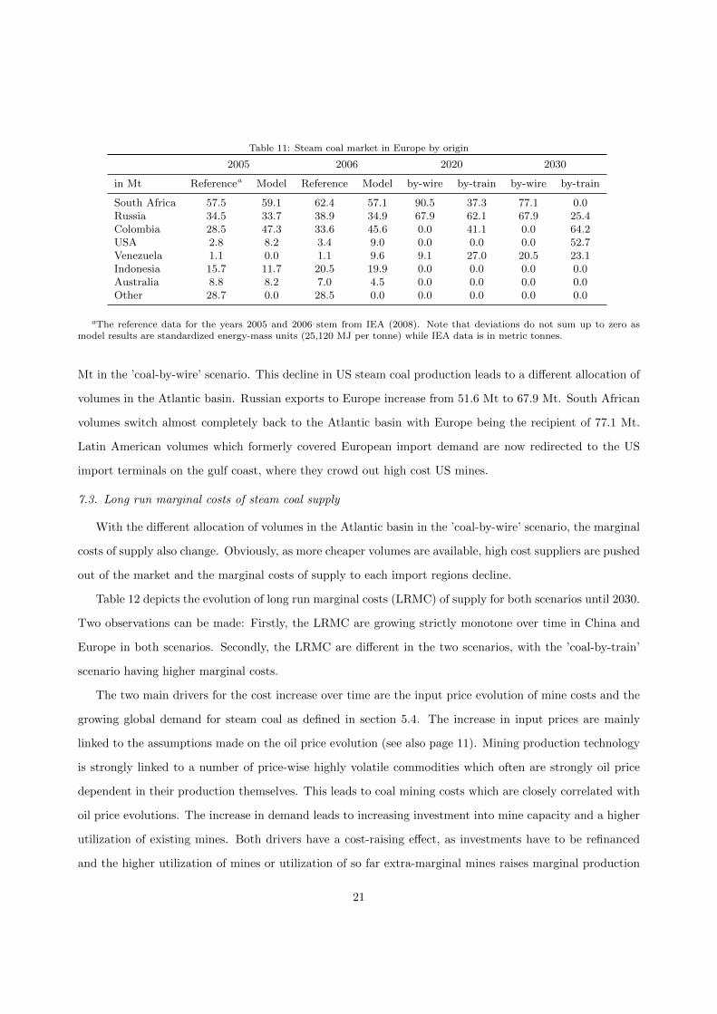
Table 11: Steam coal market in Europe by origin
2005 2006 2020 2030
in Mt Referencea Model Reference Model by-wire by-train by-wire by-train
South Africa 57.5 59.1 62.4 57.1 90.5 37.3 77.1 0.0Russia 34.5 33.7 38.9 34.9 67.9 62.1 67.9 25.4Colombia 28.5 47.3 33.6 45.6 0.0 41.1 0.0 64.2USA 2.8 8.2 3.4 9.0 0.0 0.0 0.0 52.7Venezuela 1.1 0.0 1.1 9.6 9.1 27.0 20.5 23.1Indonesia 15.7 11.7 20.5 19.9 0.0 0.0 0.0 0.0Australia 8.8 8.2 7.0 4.5 0.0 0.0 0.0 0.0Other 28.7 0.0 28.5 0.0 0.0 0.0 0.0 0.0
aThe reference data for the years 2005 and 2006 stem from IEA (2008). Note that deviations do not sum up to zero asmodel results are standardized energy-mass units (25,120 MJ per tonne) while IEA data is in metric tonnes.
Mt in the ’coal-by-wire’ scenario. This decline in US steam coal production leads to a different allocation of
volumes in the Atlantic basin. Russian exports to Europe increase from 51.6 Mt to 67.9 Mt. South African
volumes switch almost completely back to the Atlantic basin with Europe being the recipient of 77.1 Mt.
Latin American volumes which formerly covered European import demand are now redirected to the US
import terminals on the gulf coast, where they crowd out high cost US mines.
7.3. Long run marginal costs of steam coal supply
With the different allocation of volumes in the Atlantic basin in the ’coal-by-wire’ scenario, the marginal
costs of supply also change. Obviously, as more cheaper volumes are available, high cost suppliers are pushed
out of the market and the marginal costs of supply to each import regions decline.
Table 12 depicts the evolution of long run marginal costs (LRMC) of supply for both scenarios until 2030.
Two observations can be made: Firstly, the LRMC are growing strictly monotone over time in China and
Europe in both scenarios. Secondly, the LRMC are different in the two scenarios, with the ’coal-by-train’
scenario having higher marginal costs.
The two main drivers for the cost increase over time are the input price evolution of mine costs and the
growing global demand for steam coal as defined in section 5.4. The increase in input prices are mainly
linked to the assumptions made on the oil price evolution (see also page 11). Mining production technology
is strongly linked to a number of price-wise highly volatile commodities which often are strongly oil price
dependent in their production themselves. This leads to coal mining costs which are closely correlated with
oil price evolutions. The increase in demand leads to increasing investment into mine capacity and a higher
utilization of existing mines. Both drivers have a cost-raising effect, as investments have to be refinanced
and the higher utilization of mines or utilization of so far extra-marginal mines raises marginal production
21
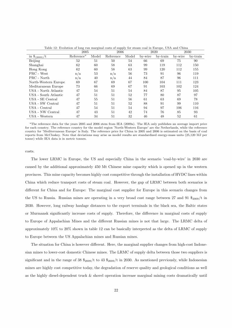
Table 12: Evolution of long run marginal costs of supply for steam coal in Europe, USA and China
2005 2006 2020 2030
in $(2009)/t Referencea Model Reference Model by-wire by-train by-wire by-train
Beijing 52 51 50 54 66 69 75 90Shanghai 62 60 58 63 99 119 112 150Hong Kong 62 60 58 63 99 120 112 155PRC - West n/a 53 n/a 56 73 91 96 119PRC - North n/a 40 n/a 44 84 87 96 111North-Western Europe 69 67 69 67 100 104 111 123Meditaranean Europe 73 66 69 67 91 103 102 124USA - North Atlantic 47 54 51 54 84 87 95 105USA - South Atlantic 47 51 51 52 77 80 87 97USA - SE Central 47 55 51 56 61 63 69 78USA - SW Central 47 51 51 52 88 91 99 110USA - Central 47 54 51 54 94 97 106 116USA - NW Central 47 43 51 42 74 76 85 93USA - Western 47 34 51 32 46 48 52 61
aThe reference data for the years 2005 and 2006 stem from IEA (2009a). The IEA only publishes an average import pricefor each country. The reference country for the model region ’North-Western Europe’ are the Netherlands, while the referencecountry for ’Mediterranean Europe’ is Italy. The reference price for China in 2005 and 2006 is estimated on the basis of coalreports from McCloskey. Note that deviations may arise as model results are standardized energy-mass units (25,120 MJ pertonne) while IEA data is in metric tonnes.
costs.
The lower LRMC in Europe, the US and especially China in the scenario ’coal-by-wire’ in 2030 are
caused by the additional approximately 450 Mt Chinese mine capacity which is opened up in the western
provinces. This mine capacity becomes highly cost competitive through the installation of HVDC lines within
China which reduce transport costs of steam coal. However, the gap of LRMC between both scenarios is
different for China and for Europe: The marginal cost supplier for Europe in this scenario changes from
the US to Russia. Russian mines are operating in a very broad cost range between 27 and 91 $2009/t in
2030. However, long railway haulage distances to the export terminals in the black sea, the Baltic states
or Murmansk significantly increase costs of supply. Therefore, the difference in marginal costs of supply
to Europe of Appalachian Mines and the different Russian mines is not that large. The LRMC delta of
approximately 10% to 20% shown in table 12 can be basically interpreted as the delta of LRMC of supply
to Europe between the US Appalachian mines and Russian mines.
The situation for China is however different. Here, the marginal supplier changes from high-cost Indone-
sian mines to lower-cost domestic Chinese mines. The LRMC of supply delta between those two suppliers is
significant and in the range of 38 $2009/t to 43 $2009/t in 2030. As mentioned previously, while Indonesian
mines are highly cost competitive today, the degradation of reserve quality and geological conditions as well
as the highly diesel-dependent truck & shovel operation increase marginal mining costs dramatically until
22
coal‐by‐train
Atlantic Basin
coal‐by‐train
Atlantic Basin
China ‐ East Invest
China ‐ West Invest
Rest of Pacific Basincoal‐by‐wire
coal‐by‐train
Atlantic Basin
China ‐ East Invest
China ‐ West Invest
Rest of Pacific Basin
0 500 1000 1500 2000 2500
coal‐by‐wire
coal‐by‐train
Mt
Atlantic Basin
China ‐ East Invest
China ‐ West Invest
Rest of Pacific Basin
0 500 1000 1500 2000 2500
coal‐by‐wire
coal‐by‐train
Mt
Atlantic Basin
China ‐ East Invest
China ‐ West Invest
Rest of Pacific Basin
0 500 1000 1500 2000 2500
coal‐by‐wire
coal‐by‐train
Mt
Atlantic Basin
China ‐ East Invest
China ‐ West Invest
Rest of Pacific Basin
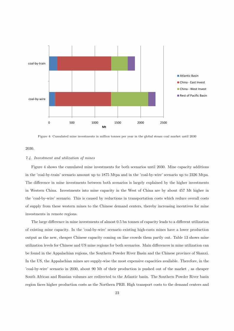
Figure 4: Cumulated mine investments in million tonnes per year in the global steam coal market until 2030
2030.
7.4. Investment and utilization of mines
Figure 4 shows the cumulated mine investments for both scenarios until 2030. Mine capacity additions
in the ’coal-by-train’ scenario amount up to 1875 Mtpa and in the ’coal-by-wire’ scenario up to 2326 Mtpa.
The difference in mine investments between both scenarios is largely explained by the higher investments
in Western China. Investments into mine capacity in the West of China are by about 457 Mt higher in
the ’coal-by-wire’ scenario. This is caused by reductions in transportation costs which reduce overall costs
of supply from these western mines to the Chinese demand centers, thereby increasing incentives for mine
investments in remote regions.
The large difference in mine investments of almost 0.5 bn tonnes of capacity leads to a different utilization
of existing mine capacity. In the ’coal-by-wire’ scenario existing high-costs mines have a lower production
output as the new, cheaper Chinese capacity coming on line crowds them partly out. Table 13 shows mine
utilization levels for Chinese and US mine regions for both scenarios. Main differences in mine utilization can
be found in the Appalachian regions, the Southern Powder River Basin and the Chinese province of Shanxi.
In the US, the Appalachian mines are supply-wise the most expensive capacities available. Therefore, in the
’coal-by-wire’ scenario in 2030, about 90 Mt of their production is pushed out of the market , as cheaper
South African and Russian volumes are redirected to the Atlantic basin. The Southern Powder River basin
region faces higher production costs as the Northern PRB. High transport costs to the demand centers and
23
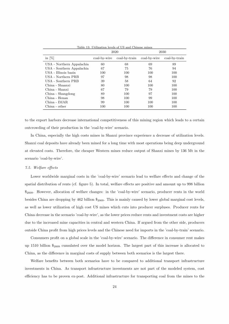
Table 13: Utilization levels of US and Chinese mines
2020 2030
in [%] coal-by-wire coal-by-train coal-by-wire coal-by-train
USA - Northern Appalachia 60 68 69 89USA - Southern Appalachia 67 75 76 94USA - Illinois basin 100 100 100 100USA - Northern PRB 97 98 98 100USA - Southern PRB 39 58 64 92China - Shaanxi 80 100 100 100China - Shanxi 67 79 79 100China - Shangdong 89 100 97 100China - Henan 98 100 99 100China - IMAR 99 100 100 100China - other 100 100 100 100
to the export harbors decrease international competitiveness of this mining region which leads to a certain
outcrowding of their production in the ’coal-by-wire’ scenario.
In China, especially the high costs mines in Shanxi province experience a decrease of utilization levels.
Shanxi coal deposits have already been mined for a long time with most operations being deep underground
at elevated costs. Therefore, the cheaper Western mines reduce output of Shanxi mines by 136 Mt in the
scenario ’coal-by-wire’.
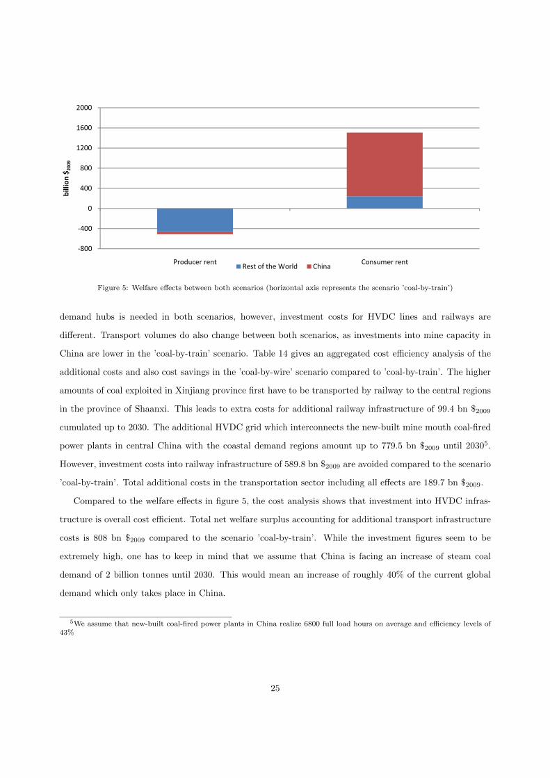
7.5. Welfare effects
Lower worldwide marginal costs in the ’coal-by-wire’ scenario lead to welfare effects and change of the
spatial distribution of rents (cf. figure 5). In total, welfare effects are positive and amount up to 998 billion
$2009. However, allocation of welfare changes: in the ’coal-by-wire’ scenario, producer rents in the world
besides China are dropping by 462 billion $2009. This is mainly caused by lower global marginal cost levels,
as well as lower utilization of high cost US mines which cuts into producer surpluses. Producer rents for
China decrease in the scenario ’coal-by-wire’, as the lower prices reduce rents and investment costs are higher
due to the increased mine capacities in central and western China. If argued from the other side, producers
outside China profit from high prices levels and the Chinese need for imports in the ’coal-by-train’ scenario.
Consumers profit on a global scale in the ’coal-by-wire’ scenario. The difference in consumer rent makes
up 1510 billion $2009 cumulated over the model horizon. The largest part of this increase is allocated to
China, as the difference in marginal costs of supply between both scenarios is the largest there.
Welfare benefits between both scenarios have to be compared to additional transport infrastructure
investments in China. As transport infrastructure investments are not part of the modeled system, cost
efficiency has to be proven ex-post. Additional infrastructure for transporting coal from the mines to the
24
0
400
800
1200
1600
2000
billi
on $
2009
‐800
‐400
0
400
800
1200
1600
2000
Producer rent Consumer rent
billi
on $
2009
Rest of the World China
Figure 5: Welfare effects between both scenarios (horizontal axis represents the scenario ’coal-by-train’)
demand hubs is needed in both scenarios, however, investment costs for HVDC lines and railways are
different. Transport volumes do also change between both scenarios, as investments into mine capacity in
China are lower in the ’coal-by-train’ scenario. Table 14 gives an aggregated cost efficiency analysis of the
additional costs and also cost savings in the ’coal-by-wire’ scenario compared to ’coal-by-train’. The higher
amounts of coal exploited in Xinjiang province first have to be transported by railway to the central regions
in the province of Shaanxi. This leads to extra costs for additional railway infrastructure of 99.4 bn $2009
cumulated up to 2030. The additional HVDC grid which interconnects the new-built mine mouth coal-fired
power plants in central China with the coastal demand regions amount up to 779.5 bn $2009 until 20305.
However, investment costs into railway infrastructure of 589.8 bn $2009 are avoided compared to the scenario
’coal-by-train’. Total additional costs in the transportation sector including all effects are 189.7 bn $2009.
Compared to the welfare effects in figure 5, the cost analysis shows that investment into HVDC infras-
tructure is overall cost efficient. Total net welfare surplus accounting for additional transport infrastructure
costs is 808 bn $2009 compared to the scenario ’coal-by-train’. While the investment figures seem to be
extremely high, one has to keep in mind that we assume that China is facing an increase of steam coal
demand of 2 billion tonnes until 2030. This would mean an increase of roughly 40% of the current global
demand which only takes place in China.
5We assume that new-built coal-fired power plants in China realize 6800 full load hours on average and efficiency levels of43%
25
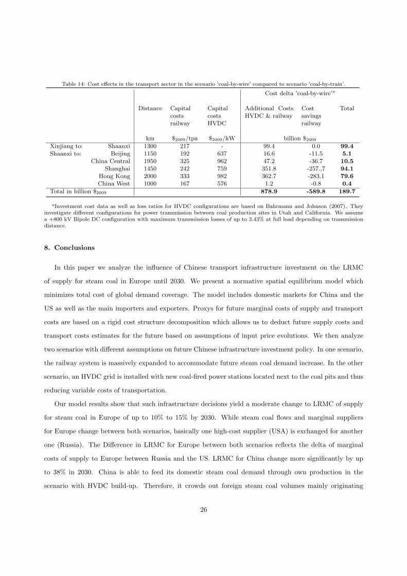
Table 14: Cost effects in the transport sector in the scenario ’coal-by-wire’ compared to scenario ’coal-by-train’.
Cost delta ’coal-by-wire’a
Distance Capitalcostsrailway
CapitalcostsHVDC
Additional CostsHVDC & railway
Costsavingsrailway
Total
km $2009/tpa $2009/kW billion $2009
Xinjiang to: Shaanxi 1300 217 - 99.4 0.0 99.4Shaanxi to: Beijing 1150 192 637 16.6 -11.5 5.1
China Central 1950 325 962 47.2 -36.7 10.5Shanghai 1450 242 759 351.8 -257.,7 94.1
Hong Kong 2000 333 982 362.7 -283.1 79.6China West 1000 167 576 1.2 -0.8 0.4
Total in billion $2009 878.9 -589.8 189.7
aInvestment cost data as well as loss ratios for HVDC configurations are based on Bahrmann and Johnson (2007). Theyinvestigate different configurations for power transmission between coal production sites in Utah and California. We assumea +800 kV Bipole DC configuration with maximum transmission losses of up to 3.43% at full load depending on transmissiondistance.
8. Conclusions
In this paper we analyze the influence of Chinese transport infrastructure investment on the LRMC
of supply for steam coal in Europe until 2030. We present a normative spatial equilibrium model which
minimizes total cost of global demand coverage. The model includes domestic markets for China and the
US as well as the main importers and exporters. Proxys for future marginal costs of supply and transport
costs are based on a rigid cost structure decomposition which allows us to deduct future supply costs and
transport costs estimates for the future based on assumptions of input price evolutions. We then analyze
two scenarios with different assumptions on future Chinese infrastructure investment policy. In one scenario,
the railway system is massively expanded to accommodate future steam coal demand increase. In the other
scenario, an HVDC grid is installed with new coal-fired power stations located next to the coal pits and thus
reducing variable costs of transportation.
Our model results show that such infrastructure decisions yield a moderate change to LRMC of supply
for steam coal in Europe of up to 10% to 15% by 2030. While steam coal flows and marginal suppliers
for Europe change between both scenarios, basically one high-cost supplier (USA) is exchanged for another
one (Russia). The Difference in LRMC for Europe between both scenarios reflects the delta of marginal
costs of supply to Europe between Russia and the US. LRMC for China change more significantly by up
to 38% in 2030. China is able to feed its domestic steam coal demand through own production in the
scenario with HVDC build-up. Therefore, it crowds out foreign steam coal volumes mainly originating
26
from South Africa and Indonesia. LRMC are then determined by lower cost Chinese mines which subsitute
high cost Indonesian mines as the marginal supplier. Thus, a large-scale HVDC grid would not only allow
China to be still independent from foreign coal imports by 2030, but also stabilize marginal costs of supply.
Welfare effects through investments into HVDC infrastructure are clearly positive even if the difference in
transport investment costs for HVDC lines is taken into account. Nevertheless, the transport investment
cost estimates outlined for both scenarios show that China is facing a challenge of enormous proportions in
terms of financing and coordination to cover its growing energy demand.
Of course, these model results are prone to assumptions we have taken: The results for the LRMC for
Europe depend strongly on the amount of US coal available from the Appalachian regions in 2030. As Hook
and Aleklett (2009) and Hook and Aleklett (2010) state, recent history shows that productivity is declining
rapidly in those regions as the best deposits have been almost exploited. Furthermore, US policy regarding
carbon emissions as well as environmental concerns could put US coal mining into a different position in
the future. As European costs of supply are based on Appalachian coal in the scenario ’coal-by-train’, an
increase in US production costs or a tightening of US volumes would change model results significantly, and
would probably increase marginal costs of supply for Europe.
Furthermore, we assume that transportation capacity, regardless if it is railway or if it is HVDC trans-
mission, is available on time. We do not model what would happen if transport bottlenecks arise in China
when railways are not expanded on time due to lack of national transport infrastructure planning. This
point is especially important, as transport infrastructure projects typically have long lead times of several
years. In the case of domestic transport bottlenecks, China would have to acquire even larger amounts of
steam coal on the international trade market, which would lead to significantly higher marginal costs in the
Pacific and the Atlantic basin due to the relative size of Chinese domestic demand compared to the trade
market volume.
An important aspect is that, under the assumptions made, China may still be able to cover its steam
coal demand by own production in 2030. But this would mean a drastic change in Chinese energy politics:
As for example mentioned in MIT (2007), China’s national bureaucratic institutions engaged in energy are
fragmented and do not coordinate well. Aspects like setting electricity and fuel prices, as well as the approval
of large infrastructure investment projects are divided into many different departments. The weakness of
central Chinese institutions promotes that currently decisions regarding the energy system in China are
often taken on the grass-roots level. On the local scale, utility companies, governments and other private
companies define the scope of energy-related decisions. To give such a large-scale national infrastructure
27
investment project any chance of realization, the national government would have to cut into this well-
established webs of local decision makers and form a national energy planning institution which yields
enough executive power to bring local agencies into line.
References
ABARE, 2008. Minerals and energy - major development projects. Tech. rep., ABARE.Abbey, D. S., Kolstad, C. D., 1983. The structure of international steam coal markets. Natural Resources Journal 23, 859–892.ABS, 2006. Producer and international trade price indexes: Concepts, sources and methods. Tech. rep., Australian Bureau of
Statistics.Bahrmann, M. P., Johnson, B. K., 2007. The abcs of hvdc transmission technologies. IEEE Power & Energy Magazine, 32–44.Baruya, P., 2007. Supply costs for internationally traded steam coal. Tech. rep., IEA Clean Coal Centre.Baruya, P., 2009. Prospects for coal and clean coal technologies in indonesia. Tech. rep., IEA Clenac Coal Centre.Bayer, A., Rademacher, M., Rutherford, A., 2009. Development and perspectives of the australian coal supply chain and
implications for the export market. Zeitschrift fuer Energiewirtschaft 2, 255–267.BGR, 2008. Reserves, Resources and Availability of Energy Resources. Federal Institute for Geosciences and Natural Resources.BP, 2010. BP Statistical Review of World Energy 2010. BP.Crocker, G., Kowalchuk, A., 2008. Prospects for coal and clean coal in russia. Tech. rep., IEA Clean Coal Centre.Dorian, J. P., 2005. Central asia: A major emerging energy player in the 21st century. Energy Policy 34, 544–555.EIA, 2010a. Annual Energy Outlook 2010. DOE/EIA.EIA, 2010b. International Energy Outlook 2010. EIA.Eichmueller, P., 2010. A model based scenario analysis of the domestic us american and chinese steam coal market - with refer-
ence to production, transportation and demand. Master’s thesis, Department of Economics and Social Sciences - Universityof Cologne.
Golombek, R., Gjelsvik, E., 1995. Effects of liberalizing the natural gas markets in western europe. The Energy Journal 16,85–112.
Haftendorn, C., Holz, F., 2010. Modeling and analysis of the international steam coal trade. Energy Journal 31 (4), 205–230.Harker, P. T., 1984. A variational inequality approach for the determintation of oligopolistic market equilibrium. Mathematical
Programming 30, 105–111.Harker, P. T., 1986. Alternative models of spatial competition. Operations Research 34 No. 3, 410–425.Hook, M., Aleklett, K., 2009. Historical trends in american coal production and a possible future outlook. International Journal
of Coal Geology 78, 201–216.Hook, M., Aleklett, K., 2010. Trends in u.s. recoverable coal supply - estimates and future production outlooks. Natural
Resources Research 19, 189–208.IEA, 2003. World Energy Investment Outlook. IEA Publications.IEA, 2008. IEA Coal Information 2008. IEA Publications.IEA, 2009a. Coal Information 2009. IEA Publications.IEA, 2009b. World Energy Outlook 2009. IEA Publications.Kolstad, C. D., 1984. The effect of market conduct on international steam coal trade. European Economic Review 24, 39–59.Kopal, C., 2008. Entwicklung und perspektive von angebot und nachfrage am steinkohlenweltmarkt. Zeitschrift fuer En-
ergiewirtschaft 3, 15–34.Labys, W. C., Yang, C. W., 1980. A quadratic programming model of the appalachian steam coal market. Energy Economics
2, 86–95.Li, R., 2008. International steam coal market integration. Tech. rep., Department of Economics, Macquarie University, Australia.Meister, W., 2008. Cost trends in coal mining. In: Coaltrans 2008.Minchener, A. J., 2004. Coal in china. Tech. rep., IEA Clean Coal Centre.Minchener, A. J., 2007. Coal supply challenges for china. Tech. rep., IEA Clean Coal Centre.MIT, 2007. The Future of Coal - Options for a Carbon-constrained World. MIT.PRC, 2006. China Coal Industry Yearbook. PRC Statistical press.PRC, 2007. China Statistical Yearbook 2006-2008. PRC Statistical Press.PRC, 2008. China Energy Yearbook 2008. PRC Statistical Press.PRC, 2010. Interprovincial coal transportation in the prc. Tech. rep., Chinese Ministry of Raiway, Beijing.Qingyun, Y., 2005. Present state and application prospects of ultra hvdc transmission in china. Power System Technology 14.Ritschel, W., 2009a. German coal importers’ association - annual report 2008/09. Tech. rep., German Coal Importers’ Associ-
ation.Ritschel, W., 2009b. Kohleweltmarkt stuetzt sich nur auf ganz wenige exportfaehige laender. In: Evangelische Akademie Tutzing
- Peak Coal und Klimawandel.Ritschel, W., 2010. German coal importers’ association - annual report 2010. Tech. rep., German Coal Importers’ Association.Rutherford, T. F., 1994. Extensions of gams for complementary problems arising in applied economic analysis. Tech. rep.,
Department of Economics, University of Colorado.Samuelson, P. A., 1952. Spatial price equilibrium and linear programming. The American Economic Review 42, 283–303.Schiffer, H.-W., Ritschel, W., 2007. World Market for Hard Coal 2007. RWE.
28

Takayama, T., Judge, G. G., 1964. Equilibrium among spatially separated markets: A reformulation. Econometrica 32, 510–524.Taoa, Z., Li, M., 2007. What is the limit of chinese coal suppliesa stella model of hubbert peak. Energy Policy 35, 3145–3154.Trueby, J., 2009. Eine modellbasierte untersuchung des kesselkohlenweltmarkts: Szenarien fr die entwicklung der grenzkosten.
Master’s thesis, Department of Economics and Social Sciences, University of Cologne.Warell, L., 2006. Market integration in the international coal industry: A cointegration approach. Energy Journal 27 (1),
99–118.Yang, C. W., Hwang, M. J., Sohng, S. N., 2002. The cournot competition in the spatial equilibrium model. Energy Economics
24, 139–154.Yinbiao, S., 2004. Present status and prospect of hvdc transmission in china. High Voltage Engineering 11.
29