Global-scale flow routing using a source-to-sink algorithm

Francisco OliveraCenter for Research in Water Resources, University of Texas at Austin

James Famiglietti1Department of Geological Sciences, University of Texas at Austin

Kwabena AsanteCenter for Research in Water Resources, University of Texas at Austin

Abstract. In this paper, the development and global application of a new approach tolarge-scale river routing is described. It differs from previous methods by the extent towhich the information content of high-resolution global digital elevation models isexploited in a computationally efficient framework. The model transports runoff directlyfrom its source of generation in a land model cell to its sink on a continental margin or inan internally draining basin (and hence is referred to as source-to-sink routing) ratherthan from land cell to land cell (which we call cell-to-cell routing). It advances thedevelopment of earlier source-to-sink models by allowing for spatially distributed flowvelocities, attenuation coefficients, and loss parameters. The method presented here hasbeen developed for use in climate system models, with a specific goal of generatinghydrographs at continental margins for input into an ocean model. However, the source-to-sink approach is flexible and can be applied at any space-time scale and in a number ofother types of large-scale hydrological and Earth system models. Hydrographs for some ofthe world’s major river basins resulting from a global application, as well as hydrographsfor the Nile River from a more detailed application, are discussed.

1. Introduction

Large-scale river-routing algorithms are required for a rangeof modeling applications in global hydrology and Earth systemscience, including macroscale hydrological modeling, fully cou-pled land-ocean-atmosphere climate system modeling, terres-trial biogeochemical and ecosystem modeling, and dynamicglobal vegetation modeling. Their purpose is to simulate thetransport of runoff generated within modeling units on land(e.g., grid cells, watersheds, or other spatially defined units),through river networks, across the landscape, to its associateddelivery point on the continental margin in order to producerealistic streamflow hydrographs at any location along thelength of the channel. While the representation of the verticalmovement of moisture through the soil-vegetation-atmospheresystem has received considerable attention in large-scale mod-eling efforts [Henderson-Sellers et al., 1993], lateral transporthas received comparatively less.

Because streamflow is an integral component of the climatesystem, the absence of river-routing algorithms in Earth systemmodels represents a significant shortcoming. For example, wa-ter cycle closure is required in fully coupled climate systemmodels (CSMs) (e.g., to maintain global freshwater and oce-anic salinity balances), yet the representation of river transportthat effectively closes the cycle is often primitive or nonexistent

[Boville and Gent, 1998]. River routing provides a means fortransport of not only water but sediment, nutrients, and bio-geochemical materials as well, all of which are important ele-ments of Earth system cycles on land: Hence their river-bornetransport requires an appropriate model representation ofstreamflow routing. From a model verification perspective,streamflow is the most observable and well documented of theland surface fluxes. Because streamflow from continental wa-tersheds represents the outflow of water from vast regions ofland surface, it is an expression of the integrated response ofthe land to all the Earth system processes occurring withinbasin boundaries. Consequently, large-scale river routing pro-vides an opportunity to better validate model simulations ofterrestrial hydrology, ecology, biogeochemistry, and climate.

The availability of high-resolution global digital elevationmodels (DEMs) like the 5-arc-min TerrainBase [Row et al.,1995] or the 30-arc-sec GTOPO30 [Gesch et al., 1999] offers animportant opportunity to advance the development of large-scale routing models by enabling progressively more realisticrepresentations of topography and river channel networks. Inthis regard, Oki and Sud [1998] have developed a global rasterriver network with a resolution of 18 3 18 using vector mapsand DEM high-resolution data. However, a significant chal-lenge is to determine how the relatively high resolution topo-graphic data can be utilized to enhance river routing algo-rithms that can be interactively coupled to regional and globalclimate models, which typically operate at coarser scales (e.g.,0.58 at high resolution to 48 3 58 at low resolution), withoutsignificantly increasing the often large computational overheadof the host models.

The purpose of this paper is to describe the development

1Also at Center for Research in Water Resources, University ofTexas at Austin.

Copyright 2000 by the American Geophysical Union.

Paper number 2000WR900113.0043-1397/00/2000WR900113$09.00

WATER RESOURCES RESEARCH, VOL. 36, NO. 8, PAGES 2197–2207, AUGUST 2000

2197

and global application of a new approach to large-scale riverrouting. The model transports runoff directly from its source ofgeneration in a land model unit to its sink on a continentalmargin or in an internally draining basin (and hence is referredto as source-to-sink routing) rather than from land cell to landcell (which we call cell-to-cell routing). It differs from mostprevious methods by the extent to which the information con-tent of high-resolution global DEMs is exploited; it advancesthe development of earlier source-to-sink models by allowingfor spatially distributed flow velocities, flow attenuation coef-ficients, and loss parameters; and it is computationally moreefficient than cell-to-cell models. The method presented herehas been developed for use in CSMs, with a specific goal ofgenerating hydrographs at continental margins for input intoan ocean model, so that the importance of water cycle closurein coupled land-ocean-atmosphere models can be properly as-sessed. However, the source-to-sink approach is flexible andcan be applied at any space-time scale and in a number of othertypes of large-scale hydrological and Earth system models.

2. Previous WorkLarge-scale flow-routing models can be classified into two

main groups: cell-to-cell models in which flow accounting oc-curs within each modeling unit and source-to-sink models inwhich flow accounting occurs only between the land source andits outlet point on the continental margin. In this section,previous models, their advantages and disadvantages, and ap-plicability are briefly discussed.

2.1. Cell-to-Cell Routing

Most previous efforts at large-scale river routing have em-ployed the cell-to-cell technique, which consists of determiningthe amount of water that flows from each land model cell to itsneighbor downstream cell and tracking it over the river net-work [Vorosmarty et al., 1989; Liston et al., 1994; Miller et al.,1994; Sausen et al., 1994; Coe, 1997; Hagemann and Dumenil,1998; Branstetter and Famiglietti, 1999]. This method invokesthe principle of continuity to derive a mass balance of waterstored within a land model cell, given, for example, by

dSi~t!dt 5 O

j

I j2i~t! 2 Oi~t! 1 Ri~t! 2 Ei~t! , (1)

where Si [L3] is the volume stored in cell i , t [T] is time,Ij2i[L3/T] is the inflow to cell i from each of the immediatelyupstream neighbor cells j , Oi[L3/T] is the outflow from cell i ,Ri [L3/T] is the runoff generated within cell i , and Ei [L3/T]are the losses due to evaporation and infiltration from the rivernetwork within cell i . Note that the term Ei accounts for lossesduring the routing process after the runoff has been generated.Outflow from the cell is typically modeled using a linear res-ervoir, where Si 5 Ki Oi and Ki [T] is a parameter whichrepresents the residence time in cell i . Determination of Ki hasbeen further studied by Vorosmarty et al. [1989] to account forfloodplain storage, by Liston et al. [1994] to account forgroundwater flow, by Coe [1997] to include lakes and wetlands,and by Hagemann and Dumenil [1998] to incorporate a cascadeof linear reservoirs rather than a single storage component.

Advantages of cell-to-cell schemes include the ease withwhich they can be implemented globally (e.g., Miller et al.[1994], Sausen et al. [1994], Coe [1997], Hagemann and Dume-nil [1998], Branstetter and Famiglietti [1999], and Fekete et al.

[1999] have all reported reasonable results in global applica-tions) and explicitly account for the volume of river water ineach cell. This second advantage enables hydrograph compu-tation for any land cell of interest. Additionally, if the volumeof river water stored in the cell can be transformed into afraction of land area covered by surface water (i.e., wetlands,floodplain storage, rivers, lakes, or reservoirs [Coe, 1997]),then the effect of that surface water on land-atmosphere in-teraction can be simulated by the climate model [Bates et al.,1993; Hostetler et al., 1993, 1994; Bonan, 1995].

However, cell-to-cell routing schemes possess some signifi-cant disadvantages that, in part, have motivated the presentresearch. Primary among these is that the cell-to-cell methoddoes not account for within-cell routing, which clearly impactsthe outflow hydrograph for the coarser grid associated withclimate models [see, e.g., Naden, 1993]. In other words, it doesnot consider the routing of water from the different areas ofthe cell to the cell outlet, from which it is routed to its down-stream cell. In order to capture these important within-celleffects, due to higher-resolution variations in topography thatdefine river networks, cell-to-cell algorithms could simply berun at the higher resolution of currently available global DEMs(e.g., roughly 1 km for GTOPO30). However, because thereare more than 90,000 DEM cells in a typical climate model cell(i.e., approximately 2.88 resolution), this is computationallyinfeasible for routing schemes that will be interactively coupledwithin climate models, given the significant computationaloverhead. Additionally, running cell-to-cell algorithms at theclimate model grid resolution also limits the accuracy withwhich river networks and watershed boundaries can be delin-eated, since grid cells have to be assigned entirely to one, andonly one, watershed. In short, cell-to-cell methods, in theircurrent form, cannot readily capitalize on the best availableglobal DEMs in order to more accurately route streamflowacross the continents into the oceans.

2.2. Source-to-Sink Routing

In their effort to develop more efficient routing models thatdo not spend resources in flow and storage calculations atlocations in which the modeler is not interested, researchersdeveloped (what is herein referred to as) source-to-sink mod-els. In the literature, researchers refer to routing from “cells inwhich runoff is produced” to “watershed outlet cells.” In thispaper, cells in which runoff is produced are called source cellsor just sources, and watershed outlet cells are called sink cellsor sinks.

Naden [1993] describes a routing method that implicitly in-cludes within-source routing (i.e., routing from the differentareas of the source to the source outlet) followed by source-to-sink routing (i.e., routing from the source outlet to thewatershed outlet). Runoff from each source is convolved witha source-specific response function to determine the contribu-tion of each source to streamflow at the sink. Total streamflowat the sink at any time is the sum of the contributions from allsources in the watershed. Although presented as a large-scalehydrologic model, the approach was only tested in a 10,000-km2 watershed. Still, according to the author, the fact thatnetwork width functions can be determined from high-resolution global DEMs using Geographic Information Sys-tems (GIS) suggests that the method is likely to be applicableglobally.

Lohman et al. [1996] employ a response function for within-source routing and the linearized St. Venant equation to trans-

OLIVERA ET AL.: GLOBAL-SCALE FLOW ROUTING2198

port streamflow from the source outflow point to the sink. Theresponse function for within-source routing is not specific toeach source and is equivalent to Mesa and Mifflin’s [1986]hillslope response. It is obtained by deconvolution of the catch-ment response function with the river network response func-tion, which is conceptually similar to the network width func-tion of Mesa and Mifflin [1986]. The scheme relies heavily onthe availability of runoff data globally for the deconvolution offunctions and, as such, may only be applicable on a regionalbasis at present (e.g., Lohman et al. [1996] test the method inthe 38,000-km2 Weser River catchment in Germany, andLohman et al. [1998] apply the scheme in the 566,000-km2

Arkansas Red River basin). However, the authors intend tosimplify and regionalize grid cell response calculations to in-crease the domain over which their approach can be applied.

Kite et al. [1994] described the development of a method thatconsists of source-to-sink routing within each source, followedby cell-to-cell routing in the watershed, and its application inthe 1,600,000-km2 Mackenzie River basin. The watershed waspartitioned into a number of sources, or grouped responseunits (GRUs), and further subdivided into five different landcover types. The distribution of travel times to the GRU outletwas computed for each land cover type by computing the traveltime from each pixel to the GRU outlet (calculated as the sumof a to-stream and in-stream travel time). Nonlinear reservoirinflow-storage and outflow-storage relationships were used totransport streamflow from GRU outlets to the next GRUdownstream. The approach described in our paper mostclosely resembles the within-GRU component of Kite et al.[1994] with important modifications and simplifications appro-priate for application at the global scale.

Advantages and disadvantages of our source-to-sink modelwith respect to the previously described routing schemes are asfollows. The first advantage is that it uses the river networktopology generated within GIS from raster high-resolutionspatial data (i.e., GTOPO30 and future higher-resolutionDEMs) and analyses it with built-in GIS tools for estimatingthe response function parameters of the lower-resolution mod-eling units used in global climate models. A second advantageis that our source-to-sink model accommodates spatially vari-able streamflow parameters. The source-to-sink models de-scribed above require uniform parameters, which is an impor-tant shortcoming for large-watershed flow routing. A thirdadvantage of the source-to-sink model presented here is thatthe streamflow parameters (i.e., flow velocity, attenuation co-efficient, and loss parameter) and the resulting hydrographsare scale-independent. This implies that the input parametersdo not have to be recalibrated when the resolution of themodeling units changes. It also implies that the accuracy of themodel results improve as the resolution of the modeling unitsincreases. This is not necessarily true for cell-to-cell models, asit has been recently demonstrated that cell resolution affectsflow attenuation [Olivera et al., 1999]. A final advantage iscomputational efficiency relative to the cell-to-cell approach.Because streamflow is transported directly from the point ofrunoff generation to the watershed outlet, routing calculationsare not required within all the land cells between these twoendpoints. The importance of this computational efficiencyincreases for larger watersheds and higher-resolution applica-tions. An important disadvantage of the source-to-sink methodis that river water stored within each cell is not explicitlytracked in time; consequently, hydrographs are only generatedat watershed outlets rather than for every cell on the land

surface as in the cell-to-cell method. Finally, because of thelinearity of the system, the source-to-sink model requires con-stant in time, but not necessarily uniform in space, flow pa-rameters (i.e., flow velocity, flow attenuation coefficient, andloss coefficient), so that response functions can be defined foreach source.

In our opinions the advantages of the source-to-sink ap-proach outweigh the disadvantages and hence justify an explo-ration of the feasibility of the approach at the global scale inthe context of an eventual coupling with a CSM. The remain-der of this paper describes the global implementation of asimple and robust source-to-sink routing scheme. A detailedintercomparison of cell-to-cell and source-to-sink methods isan active area of research by the authors, as are methods forcombining the two approaches. Results of these investigationswill be presented in future publications.

3. MethodologyThe methodology presented here models the process by

which the water moves across the landscape from the locationwhere runoff is generated, the source, to the location along thecontinental margin where no further flow routing is necessary,the sink. The model assumes that the terrain topography isdescribed by a DEM, and the runoff distribution, in space andtime, is known from a separate land surface model. It gener-ates hydrographs at the different sinks.

The model is supported by a Global Spatial Database, in theform of raster and vector GIS maps, specifically developed towork in conjunction with it. Streamflow parameters, such asvelocity, attenuation coefficients, and loss parameters, whichdepend more on local than on overall topographic conditions,are not included in the database and are left for the user todefine.

3.1. Global Spatial Database

In this section, the general principles followed to develop theGlobal Spatial Database that supports the model are ex-plained. This Global Spatial Database is available from theauthors by request.

A DEM is a sampled array of elevations for ground positionsthat usually are at regularly spaced intervals. DEM-based ter-rain analysis consists of extracting from the DEM the relevantinformation about the flow network for hydrologic modeling.GTOPO30, a set of 30-arc-sec (approximately 1 km) DEMs,was used for the hydrologic analysis because it is the highest-resolution raster topographic data available for the entireworld. The terrain analysis was carried out by applying stan-dard GIS functions included in commercially available soft-ware that supports operations on raster data.

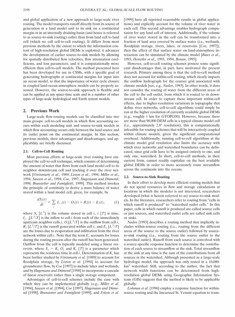
By identifying the downstream pixel adjacent to each terrainpixel, a network that represents the flow paths is produced, anda unique path can be traced from each pixel to the ocean (seeFigure 1). In order for water to flow along the landscapewithout being trapped in terrain depressions, each pixel musthave at least one of its eight neighbor pixels at a lower eleva-tion. However, in some cases, terrain models (DEMs) depictfictitious depressions, produced by the interpolation schemesused to describe variation in elevation between raster points[DeVantier and Feldman, 1993]. In general, the existence ofdepressions in the DEM is explained by (1) fictitious terraindepressions, also called pits, which might be small for mostpractical purposes but which are critical for hydrologic mod-

2199OLIVERA ET AL.: GLOBAL-SCALE FLOW ROUTING

eling, and (2) inland catchments in which the lowest pixelconstitutes a pour point (i.e., a point toward which water in thesurrounding area flows and forms lakes or ponds). Therefore,before determining the flow network, it is necessary to correctthe DEM by filling the pits up to an elevation that allows waterto flow through and by flagging the lowest pixels of the inlandcatchments (pour points) as water sinks. The methodologyused to identify inland catchments consists of filling all theDEM depressions as if they were pits and comparing the filledareas with maps of basins of the world available in the litera-ture [UNESCO, 1978; Revenga et al., 1998]. The lowest pixel ofeach of the filled areas that coincide with an inland catchmentis flagged as a water sink, and these pixels constitute the catch-ment pour points. With all the pour points identified, the DEMpits are filled, and the flow network is determined. Once theflow network has been determined, sinks and sources can bedefined.

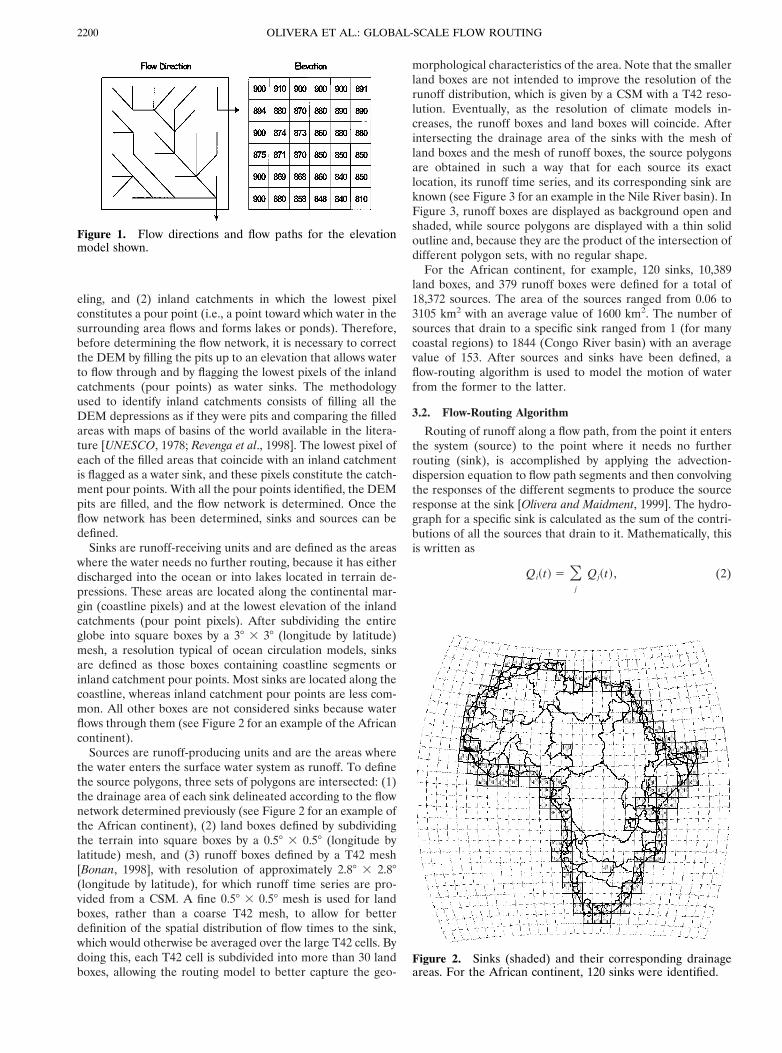
Sinks are runoff-receiving units and are defined as the areaswhere the water needs no further routing, because it has eitherdischarged into the ocean or into lakes located in terrain de-pressions. These areas are located along the continental mar-gin (coastline pixels) and at the lowest elevation of the inlandcatchments (pour point pixels). After subdividing the entireglobe into square boxes by a 38 3 38 (longitude by latitude)mesh, a resolution typical of ocean circulation models, sinksare defined as those boxes containing coastline segments orinland catchment pour points. Most sinks are located along thecoastline, whereas inland catchment pour points are less com-mon. All other boxes are not considered sinks because waterflows through them (see Figure 2 for an example of the Africancontinent).

Sources are runoff-producing units and are the areas wherethe water enters the surface water system as runoff. To definethe source polygons, three sets of polygons are intersected: (1)the drainage area of each sink delineated according to the flownetwork determined previously (see Figure 2 for an example ofthe African continent), (2) land boxes defined by subdividingthe terrain into square boxes by a 0.58 3 0.58 (longitude bylatitude) mesh, and (3) runoff boxes defined by a T42 mesh[Bonan, 1998], with resolution of approximately 2.88 3 2.88(longitude by latitude), for which runoff time series are pro-vided from a CSM. A fine 0.58 3 0.58 mesh is used for landboxes, rather than a coarse T42 mesh, to allow for betterdefinition of the spatial distribution of flow times to the sink,which would otherwise be averaged over the large T42 cells. Bydoing this, each T42 cell is subdivided into more than 30 landboxes, allowing the routing model to better capture the geo-

morphological characteristics of the area. Note that the smallerland boxes are not intended to improve the resolution of therunoff distribution, which is given by a CSM with a T42 reso-lution. Eventually, as the resolution of climate models in-creases, the runoff boxes and land boxes will coincide. Afterintersecting the drainage area of the sinks with the mesh ofland boxes and the mesh of runoff boxes, the source polygonsare obtained in such a way that for each source its exactlocation, its runoff time series, and its corresponding sink areknown (see Figure 3 for an example in the Nile River basin). InFigure 3, runoff boxes are displayed as background open andshaded, while source polygons are displayed with a thin solidoutline and, because they are the product of the intersection ofdifferent polygon sets, with no regular shape.

For the African continent, for example, 120 sinks, 10,389land boxes, and 379 runoff boxes were defined for a total of18,372 sources. The area of the sources ranged from 0.06 to3105 km2 with an average value of 1600 km2. The number ofsources that drain to a specific sink ranged from 1 (for manycoastal regions) to 1844 (Congo River basin) with an averagevalue of 153. After sources and sinks have been defined, aflow-routing algorithm is used to model the motion of waterfrom the former to the latter.

3.2. Flow-Routing Algorithm

Routing of runoff along a flow path, from the point it entersthe system (source) to the point where it needs no furtherrouting (sink), is accomplished by applying the advection-dispersion equation to flow path segments and then convolvingthe responses of the different segments to produce the sourceresponse at the sink [Olivera and Maidment, 1999]. The hydro-graph for a specific sink is calculated as the sum of the contri-butions of all the sources that drain to it. Mathematically, thisis written as

Qi~t! 5 Oj

Qj~t! , (2)

Figure 1. Flow directions and flow paths for the elevationmodel shown.

Figure 2. Sinks (shaded) and their corresponding drainageareas. For the African continent, 120 sinks were identified.

OLIVERA ET AL.: GLOBAL-SCALE FLOW ROUTING2200

where Qi(t) [L3/T] is the hydrograph of sink i , Qj(t) [L3/T]is the contribution of source j , and the sum applies to allsources that drain to sink i . In turn, Qj(t) is calculated as

Qj~t! 5 AjRj~t! p uj~t! (3)

where Aj [L2] is the area of source j , Rj(t) [L/T] is the timeseries of runoff generated at source j , uj(t) [1/T] is the re-sponse function of source j at sink i , and the asterisk stands forthe convolution integral. Assuming the response function is afirst-passage-time distribution, which is in accordance with thework of other researchers who have modeled the time spent bywater in surface water systems [Mesa and Mifflin, 1986; Naden,1992; Troch et al., 1994; Olivera and Maidment, 1999], then

uj~t! 51

2t Îp~t/t j!/P j

exp H2@1 2 ~t/t j!#

2

4~t/t j!/P jJ , (4)

where t j [T] is the average flow time and P j is a representativePeclet number for the flow path from source j to its corre-sponding sink i . Figure 4 shows first-passage-time distributionsfor different values of P j and t j 5 100 s. If, because of thespatial variability of the system, the flow path is subdivided intoa sequence of segments with different flow parameters, thenthe values of t j and P j can be calculated as [Olivera and Maid-ment, 1999]

t j 5 Ok

S 1vkD Lk, (5)

P j 5 F OkS 1

vkD LkG 2YF OkSDk

vk3D LkG , (6)

where Lk [L] is the flow distance, vk [L/T] is the flow velocity,and Dk [L2/T] is the attenuation coefficient in segment k ofthe flow path, and the sum applies to all segments of the flowpath. Note that in the context of raster terrain data, flow pathsegments are the links that connect pixels with their immediatedownstream neighbors. Thus spatially distributed flow param-eters such as flow velocity and attenuation coefficient can bestored in the same raster format as the DEM.

Since the representative Peclet number P j is a measure ofthe relative importance of advection with respect to hydrody-namic dispersion (the cause of flow attenuation), some impor-tant conclusions can be drawn from (6): the relative impor-tance of advection with respect to flow attenuation increaseswith flow path length and flow velocity and decreases with theattenuation coefficient. Therefore it is expected that flow at-tenuation plays a lesser role as the watershed size increases.

First-order losses (i.e., flow lost proportional to actual flow)can also be included in this approach by multiplying the re-sponse function of (4) by a dimensionless loss factor F j

[Olivera, 1996] (available at www.ce.utexas.edu/prof/olivera/disstn/abstract.htm) equal to

F j 5 exp H2OkS lk

vkD LkJ , (7)

where the loss parameter lk [1/T] is related to the loss mech-anisms such as evaporation to the atmosphere or infiltration tothe deep subsurface system. The loss parameter can be under-stood as the fraction of water lost per unit time and reflects thefact that losses increase with flow time and that distant sourcesexperience more losses than those located close to the sink.Note that although the loss parameter is constant, water lossesare not constant and change in time as the flow changes. Afteraccounting for losses, the source response function at the sinkis equal to

uj~t! 5F j

2t Îp~t/t j!/P j

exp H2@1 2 ~t/t j!#

2

4~t/t j!/P jJ . (8)

The summation terms in (5), (6), and (7) can be calculatedusing GIS functions. The flow distance from a DEM pixel tothe continental margin or inland catchment pour point, forexample, is calculated along the flow path according to the flow

Figure 3. Source polygons defined after intersecting thedrainage area of the sinks with the mesh of land boxes and themesh of runoff boxes. For the Nile River basin, 1120 landboxes (0.58 3 0.58 longitude by latitude) and 62 runoff boxes(T42) were identified. Large open and shaded boxes corre-spond to the runoff boxes. It can be seen that about 30 landboxes are contained in a runoff box.

Figure 4. First-passage-time distributions for a mean valueof 100 s and Peclet numbers ranging from 0.33 to 100. Notethat as the Peclet numbers increases, the responses decreasetheir standard deviation (i.e., tend to pure translation).

2201OLIVERA ET AL.: GLOBAL-SCALE FLOW ROUTING

path network determined previously and is equal to (k Lk.Similarly, the summation terms (k Lk /vk, (k Dk Lk /vk

3, and(k lk Lk /vk are calculated using the same algorithm but aftermultiplying Lk by weight factors equal to 1/vk, Dk/vk

3, andlk/vk, respectively. Therefore, after making these calculations,sources can be attributed with the average value within thepolygons of ( j Lk (flow length), (k Lk /vk (flow time),(k Dk Lk /vk

3 (attenuation), and (k lk Lk /vk (losses). Thus thesmaller the source polygons are, the less the averaging affectsthe parameters but at the expense of more computational time.

In summary, after calculating the summation terms and at-tributing the source polygons with their average values, theparameters t j, P j, and F j are determined using (5), (6), and(7). A response function for each source is then determinedusing (8). The contribution of a source at its sink is obtained byconvolving the response function and the runoff time series asin (3). Finally, the flow at the sink is calculated as the sum ofthe contributions of the sources in its drainage area as pre-sented in (2).

4. Application, Results, and DiscussionIn this section, we first demonstrate the applicability of the

model for use in global routing calculations and then highlightits power and flexibility in an application in the Nile Riverbasin.

4.1. Application to the Globe

A 10-year daily time series of T42-resolution global runoffdata, simulated using the National Center for AtmosphericResearch Community Climate Model Version 3 (CCM3)[Kiehl et al., 1998] with an interactive land surface component,the Land Surface Model Version 1 (LSM) [Bonan, 1996], wasused as input to our flow-routing model. While it is well knownthat climate model runoff does not agree well with observa-tions, Bonan [1998] and Kiehl et al. [1998] have shown improve-ment in simulated hydrology over previous CCM versions inwhich land surface conditions were prescribed. For our pur-poses, use of the CCM3 runoff output is sufficient for demon-strating the features of the routing algorithm, as this is pre-cisely the resolution and quality of runoff data that will beinput into the routing scheme when coupled to a CSM.

Routing of CSM runoff data, with specified streamflow pa-rameters, for different basins can be seen in Figure 5. The riverbasins selected were the Congo in Africa, the Amazon, Ori-noco, and Parana in South America, the Mackenzie and Mis-sissippi in North America, and the Yangtze and Huang Hu inAsia. In all cases, v 5 0.3 m/s, D 5 0, and l 5 0, whichimplies pure translation at a rate of 0.3 m/s and no losses. Notethat we have not attempted a global calibration of thesestreamflow parameters, because validating CCM3 runoff is notthe focus of this paper. Rather, our intention is to show thecapability of the model to transport streamflow over vast landregions and simulate hydrographs at continental margins forinput into ocean circulation models, given a set of streamflowparameters and simulated runoff rates.

Figure 5 shows, for all cases, lagging and damping of the flowhydrograph with respect to the runoff, so that peak flows arelower than peak runoff values, low flows are higher than lowrunoff values, and, in general, the entire flow hydrograph isshifted to the right, along the time axis, with respect to therunoff. The lags are induced by overall travel times to thecoast, and the damping is induced by the differential travel

times and by the flow attenuation processes. It can also beobserved that, depending on the size, shape, and geomorphol-ogy of the watershed, lags can be as long as 4 to 5 months anddamping can be as much as 40%. Note that these results arealso sensitive to the choice of streamflow parameters and thespatial-temporal variability of the runoff input.

Owing to inadequacies of the climate model runoff men-tioned above, we are not able to validate the imposed transla-tion and attenuation. However, the predicted hydrographs arecertainly reasonable given the realistic nature of the velocityand topographic input parameters. The impact of these delayson ocean circulation and ocean-atmosphere interaction is thesubject of ongoing research.

The power and flexibility of the routing scheme, that is, itsability to incorporate terrain spatial variability, are discussednext in an application of the model to the Nile River basinunder differing streamflow parameters.

4.2. Application to the Nile River Basin

Spatially distributed streamflow parameters, such as flowvelocity, attenuation coefficient, and loss coefficient, are diffi-cult to estimate at a global scale when detailed descriptions ofthe terrain are not available. Assumptions of uniformly distrib-uted parameters, though appealing for their simplicity, mayoverlook well-known hydrologic processes that take place insome parts of the river basins. For example, floodplain storage,which is significantly important in flat areas such as the SuddMarshes of the Nile River basin in North Africa, the InnerDelta of the Niger River basin in West Africa, and most of theAmazon River basin in South America but which is almostnegligible in mountainous areas, indicates the need for ac-counting for nonuniformly distributed parameters.

An application of the model to the Nile River basin is in-cluded next. The Nile River drains areas from nine Africancountries: Burundy, Democratic Republic of the Congo,Egypt, Eritrea, Ethiopia, Kenya, Rwanda, Sudan, and Uganda.It is a 3,250,000-km2 drainage area located in northeast Africa[Revenga et al., 1998] and extends from 228E to 408E longitudeand 38S to 338N latitude (see Figure 6). The Nile River at theMediterranean derives from the confluence of the White Nileand the Blue Nile at Khartoum, Sudan. From its uppermostheadstream, the Luvironza River in Burundi, the Nile has alength of more than 6700 km. The White Nile rises in the EastAfrican Highlands and flows predominantly northward. Alongits way toward the confluence with the Blue Nile the WhiteNile flows through a large marshy region in south Sudanknown as the Sudd Marshes. The Sudd are a 300-km-long by350-km-wide, flat, and shallow plain that drains 1,560,000 km2

and collects more than 70% of the basin precipitation. Themarshes slow down the river so that about half the inflow is lostto evaporation [Hurst and Phillips, 1938]. The Blue Nile flowsnorthwestward from the Ethiopian highlands. It drains 310,000km2 and collects approximately 15% of the precipitation of theentire basin. The Blue Nile is characterized by steep slopes,having a vertical drop of 2400 m in a distance of 1200 km.Precipitation in the Nile basin ranges from 2100 mm/yr in theBlue Nile headwaters to as much as 1200 mm/yr in the upperWhite Nile area to almost zero in northern and central Egypt.Most of the precipitation occurs during July and August,whereas December and January are relatively dry.

For the sink that captures the Nile River basin, the Medi-terranean outfall grid cell, 1808 sources were identified with areasranging from 0.12 km2 to 3105 km2 for a total of 3,350,000 km2

OLIVERA ET AL.: GLOBAL-SCALE FLOW ROUTING2202

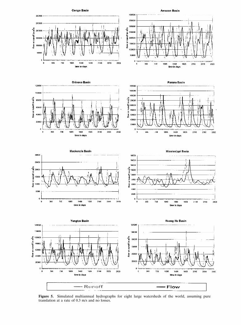
Figure 5. Simulated multiannual hydrographs for eight large watersheds of the world, assuming puretranslation at a rate of 0.3 m/s and no losses.

(see Figure 3). This area is close to that reported by Revenga et al.[1998], which was estimated using a different methodology.

In this application, emphasis has been placed on the impor-tance of accounting for the spatial variability of the streamflowparameters. For this purpose, three distinct zones were as-sumed to constitute the basin: the Blue Nile subbasin, the SuddMarshes, and the rest of the basin (see Figure 7). The BlueNile is a relatively steep area in which velocities are assumed tobe higher and attenuation coefficients are assumed to be lowerthan in the rest of the basin. In contrast, the Sudd Marshes isa swampy area in which velocities are lower, attenuation coef-ficients are higher, and loss parameters are large compared tothe rest of the basin. Losses were considered only in the SuddMarshes, which has been identified as the major area of lossesin the basin [Hurst and Phillips, 1938].

Estimation of flow velocities and loss coefficients was basedon flow observations. Observed flows [Hurst and Phillips, 1938]indicate that peak discharges take approximately 4 days totravel 418 km, along the Blue Nile, from Wad el Aies toKhartoum, that is, a flow velocity of approximately 1.2 m/s.Likewise, the White Nile takes about 3 months to travel 711km, predominantly through the Sudd Marshes in the Sudanfrom Mongalla to Malakal, that is, a velocity of about 0.1 m/s.Finally, the velocity between Malakal and Mogren, just southof Khartoum, is estimated from a distance of 794 km and atravel time of 20 days, that is, a flow velocity of approximately0.5 m/s. The value of 0.018/day for the loss coefficient in theSudd Marshes (i.e., a loss of 1.8% of the flow per day) waschosen to satisfy the condition of 50% losses in the area.Attenuation coefficients are order of magnitude estimatesbased on measured values for different river basins reported byFischer et al., [1979] and Seo and Cheong [1998]. After com-paring hydrologic characteristics of the Nile basin zones (i.e.,flow rate and slope) with those of the rivers reported in theliterature, attenuation coefficients of 300 m2/s, 4500 m2/s, and1500 m2/s were chosen for the Blue Nile, the Sudd Marshes,and the rest of the Nile basin, respectively. These parametersfall within reasonable limits for flow velocities, attenuation

coefficients and loss parameters and were chosen to demon-strate the importance of accounting for the spatial variability ofstreamflow parameters in the calculation of flows. Not all thefeatures of the basin were considered, though, since reservoirsand lakes, which are expected to have different streamflowparameters, were not considered in the present study.

Figure 8 shows the area–flow time distribution for the NileRiver basin under four different assumptions: (1) variable vand D , (2) variable v and uniform D (D 5 908 m2/s), (3)uniform v (v 5 0.43 m/s) and variable D , and (4) uniform v(v 5 0.43 m/s) and D (D 5 908 m2/s), where variable refersto the spatially differing values indicated above. For variable vand D the mean and standard deviation of the distributionwere 100 and 49 days, respectively. The velocity, v 5 0.43 m/s,used for uniform velocity analysis was chosen so that the meanof the distribution remain unaltered. The attenuation coeffi-cient, D 5 908 m2/s, used for uniform attenuation coefficientanalysis, was chosen so that the standard deviation remainunaltered when variable velocities were considered (curve 2).However, it was observed that with uniform velocities (curves3 and 4), the standard deviation dropped to 40 days. This dropin the standard deviation value results from the fact that whilethe mean of the distribution depends on v only, the standarddeviation depends on both v and D . From the physical point ofview the basin response function or instantaneous unit hydro-graph (i.e., the hydrograph at the basin outlet produced by aunit instantaneous and uniformly distributed runoff input) is arescaled version of the area–flow time distribution. That is, thebasin response function is obtained by multiplying the area (of thearea–flow time distribution) by a unit instantaneous and uni-formly distributed runoff input. The concept of response function,

Figure 6. Nile River basin in East Africa.

Figure 7. Hydrologic zones of the Nile River basin: the BlueNile subbasin (dark shading), the Sudd Marshes (hatchedarea), and the rest of the basin (medium and light shading).The Sudd Marshes contributing drainage area (shaded) isshown here for illustration purposes, but it was not treated asa different hydrologic zone.

OLIVERA ET AL.: GLOBAL-SCALE FLOW ROUTING2204

though, is not in frequent use in large-scale hydrology sinceuniformly distributed runoff inputs are unlikely in large basins.

The most striking result observed in Figure 8 is that curvesfrom the variable-velocity analysis (curves 1 and 2) and curvesfrom the uniform-velocity analysis (curves 3 and 4) group to-gether, while the differences between the curves within eachgroup are minor. Curves that correspond to variable velocityare bimodal, with a first peak deriving mostly from the BlueNile drainage area and a second deriving from the White Nile.

Spatial variability of attenuation coefficients also proved to beimportant, especially for the case of variable velocity, althoughnot as important as for flow velocity. In Figure 8, curves 1 and 2do not show much discrepancy until about day 90, when curve 1(variable v and D) became considerably smoother than curve 2(variable v and uniform D). Thus the effect of the difference inattenuation coefficients between curves 1 and 2 seems to be neg-ligible for the Blue Nile drainage area (first peak) and significantfor the White Nile drainage area (second peak). This additionalattenuation is explained by the effect of the Sudd Marshes, char-acterized by very slow velocities. Similarly, the discrepancy be-tween curves 3 (uniform v and variable D) and 4 (uniform vand D) shows up only after about day 150, when the peak andlow values of curve 4 are attenuated. Because that part of thecurve corresponds to the upper White Nile drainage area, theadditional attenuation in curve 3 is explained by the effect ofthe Sudd Marshes. Still, it can be noted that for uniform ve-locity, the effect of flow attenuation is not significant.

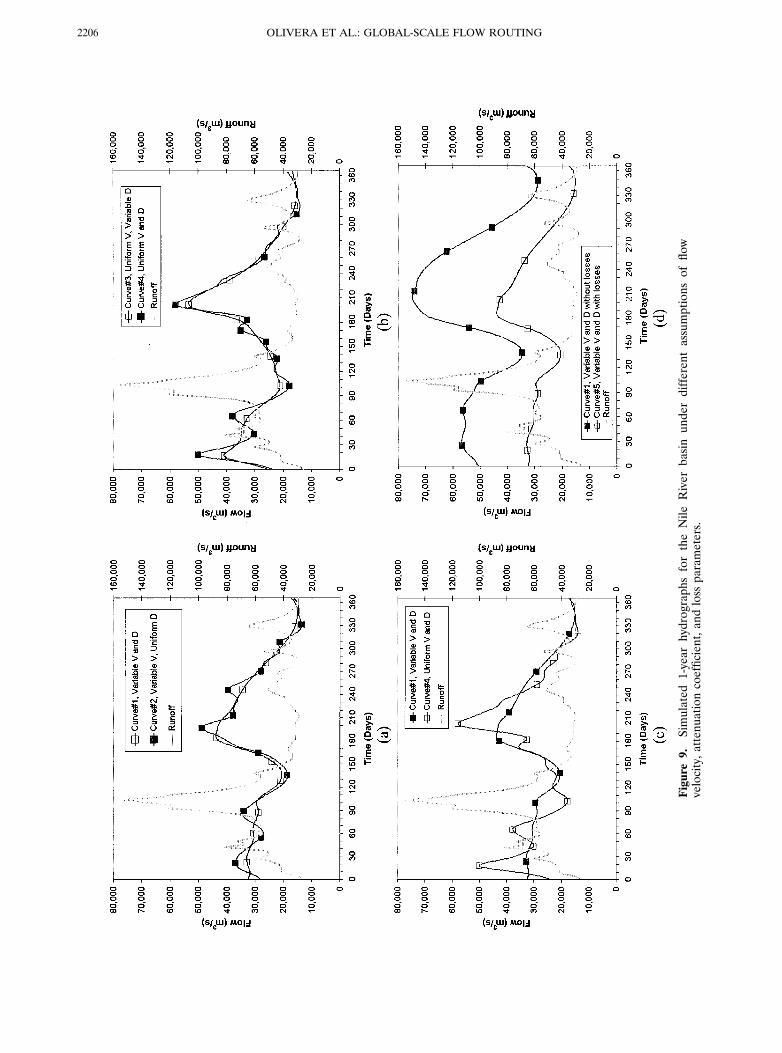
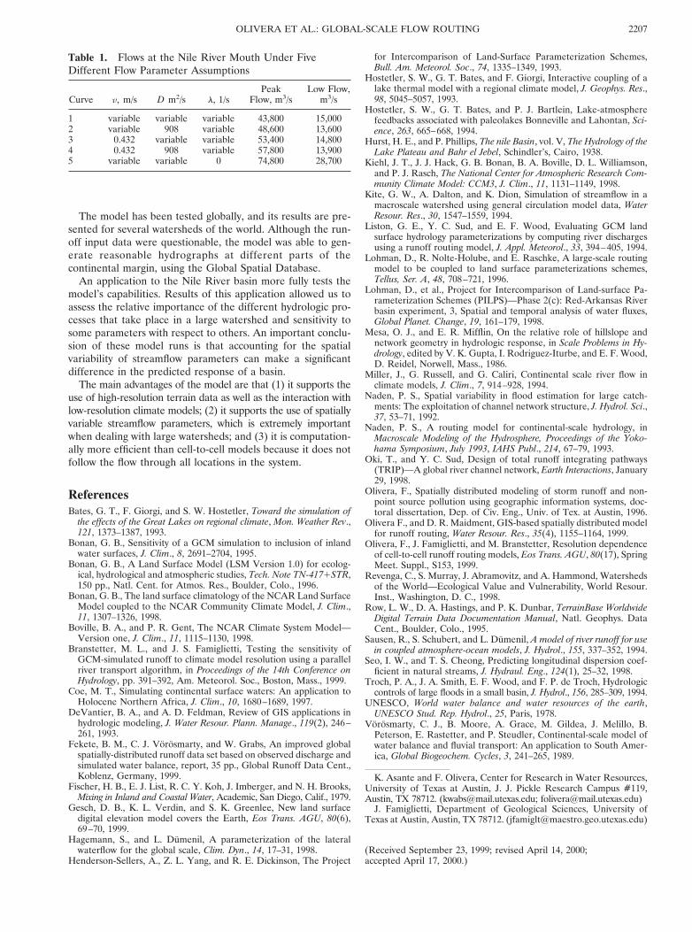
It is important to note that in the area–flow time curvesdiscussed above, the relative importance of the sources, givenby the total runoff depth and overall losses, was not consid-ered. The effect of spatial variation of runoff depth plus thetemporal distribution of runoff will be considered next whengenerating hydrographs at the ocean. Figure 9 shows 1 year offlows at the Nile River mouth resulting from running the model,with CSM runoff data, under five sets of streamflow parameters:(1) variable v, D, and l; (2) variable v, uniform D (D 5 908 m2/s),and variable l; (3) uniform v (v 5 0.43 m/s) and variable Dand l; (4) uniform v (v 5 0.43 m/s) and D (D 5 908 m2/s)and variable l; and (5) variable v and D with l 5 0, where

variable refers to the spatially distributed values indicatedabove. Table 1 summarizes the results of these five model runs.

In Figure 9a, curves 1 and 2 are compared. Averaging D witha variable velocity field results in higher peak flows and lowerlow flows. Similarly, in Figure 9b, curves 3 and 4 are compared.Again, averaging D with a uniform velocity field results in higherpeak flows and lower low flows. Finally, in Figure 9c, curves 1 and4 are compared. As might be expected, averaging both streamflowparameters results in higher peak flows and lower low flows. Inthis last case, flow volume also changes because with variablevelocity water stays longer in the Sudd Marshes and is subject togreater losses. The effect of accounting for losses in the SuddMarshes is shown in Figure 9d. It can be seen that, as an average,the flow volume decreases by about 40% when l 5 0.018/day.

The discrepancies between the hydrographs, peak flows, andlow flows in Figure 9 show the importance of accounting forlocalized areas of floodplain storage and, in general, of ac-counting for spatial variability of the terrain and streamflowparameters. The fact that a 108,000-km2 localized area offloodplain storage, like the Sudd Marshes, can modify peakflows by as much as 32% in a 3,250,000-km2 basin shows thatmodels that do not support spatially distributed streamflowparameters are limited in their applicability.

5. ConclusionsA model for runoff routing at a global, continental, or large-

watershed scale has been developed. The method presentedhere has been developed for use in CSMs, with a specific goalof generating hydrographs at continental margins for inputinto an ocean model so that the importance of large-scale rivertransport can be properly assessed. It models the transfer ofrunoff from its sources of generation (where it enters thesurface water system) to its sinks at either the continentalmargin or an inland catchment pour point (where no furtherrouting is necessary) and therefore is referred to as a source-to-sink model. The model is supported by a Global SpatialDatabase in which all sources and sinks for land areas of theentire world have been identified and properly attributed.

Figure 8. Contributing area-time distribution for the Nile River basin under different assumptions of flowvelocity and flow attenuation coefficient.

2205OLIVERA ET AL.: GLOBAL-SCALE FLOW ROUTING

Fig

ure

9.Si

mul

ated

1-ye

arhy

drog

raph

sfo

rth

eN

ileR

iver

basi

nun

der

diff

eren

tas

sum

ptio

nsof

flow

velo

city

,att

enua

tion

coef

ficie

nt,a

ndlo

sspa

ram

eter

s.

OLIVERA ET AL.: GLOBAL-SCALE FLOW ROUTING2206

The model has been tested globally, and its results are pre-sented for several watersheds of the world. Although the run-off input data were questionable, the model was able to gen-erate reasonable hydrographs at different parts of thecontinental margin, using the Global Spatial Database.

An application to the Nile River basin more fully tests themodel’s capabilities. Results of this application allowed us toassess the relative importance of the different hydrologic pro-cesses that take place in a large watershed and sensitivity tosome parameters with respect to others. An important conclu-sion of these model runs is that accounting for the spatialvariability of streamflow parameters can make a significantdifference in the predicted response of a basin.

The main advantages of the model are that (1) it supports theuse of high-resolution terrain data as well as the interaction withlow-resolution climate models; (2) it supports the use of spatiallyvariable streamflow parameters, which is extremely importantwhen dealing with large watersheds; and (3) it is computation-ally more efficient than cell-to-cell models because it does notfollow the flow through all locations in the system.

ReferencesBates, G. T., F. Giorgi, and S. W. Hostetler, Toward the simulation of

the effects of the Great Lakes on regional climate, Mon. Weather Rev.,121, 1373–1387, 1993.

Bonan, G. B., Sensitivity of a GCM simulation to inclusion of inlandwater surfaces, J. Clim., 8, 2691–2704, 1995.

Bonan, G. B., A Land Surface Model (LSM Version 1.0) for ecolog-ical, hydrological and atmospheric studies, Tech. Note TN-4171STR,150 pp., Natl. Cent. for Atmos. Res., Boulder, Colo., 1996.

Bonan, G. B., The land surface climatology of the NCAR Land SurfaceModel coupled to the NCAR Community Climate Model, J. Clim.,11, 1307–1326, 1998.

Boville, B. A., and P. R. Gent, The NCAR Climate System Model—Version one, J. Clim., 11, 1115–1130, 1998.

Branstetter, M. L., and J. S. Famiglietti, Testing the sensitivity ofGCM-simulated runoff to climate model resolution using a parallelriver transport algorithm, in Proceedings of the 14th Conference onHydrology, pp. 391–392, Am. Meteorol. Soc., Boston, Mass., 1999.

Coe, M. T., Simulating continental surface waters: An application toHolocene Northern Africa, J. Clim., 10, 1680–1689, 1997.

DeVantier, B. A., and A. D. Feldman, Review of GIS applications inhydrologic modeling, J. Water Resour. Plann. Manage., 119(2), 246–261, 1993.

Fekete, B. M., C. J. Vorosmarty, and W. Grabs, An improved globalspatially-distributed runoff data set based on observed discharge andsimulated water balance, report, 35 pp., Global Runoff Data Cent.,Koblenz, Germany, 1999.

Fischer, H. B., E. J. List, R. C. Y. Koh, J. Imberger, and N. H. Brooks,Mixing in Inland and Coastal Water, Academic, San Diego, Calif., 1979.

Gesch, D. B., K. L. Verdin, and S. K. Greenlee, New land surfacedigital elevation model covers the Earth, Eos Trans. AGU, 80(6),69–70, 1999.

Hagemann, S., and L. Dumenil, A parameterization of the lateralwaterflow for the global scale, Clim. Dyn., 14, 17–31, 1998.

Henderson-Sellers, A., Z. L. Yang, and R. E. Dickinson, The Project

for Intercomparison of Land-Surface Parameterization Schemes,Bull. Am. Meteorol. Soc., 74, 1335–1349, 1993.

Hostetler, S. W., G. T. Bates, and F. Giorgi, Interactive coupling of alake thermal model with a regional climate model, J. Geophys. Res.,98, 5045–5057, 1993.

Hostetler, S. W., G. T. Bates, and P. J. Bartlein, Lake-atmospherefeedbacks associated with paleolakes Bonneville and Lahontan, Sci-ence, 263, 665–668, 1994.

Hurst, H. E., and P. Phillips, The nile Basin, vol. V, The Hydrology of theLake Plateau and Bahr el Jebel, Schindler’s, Cairo, 1938.

Kiehl, J. T., J. J. Hack, G. B. Bonan, B. A. Boville, D. L. Williamson,and P. J. Rasch, The National Center for Atmospheric Research Com-munity Climate Model: CCM3, J. Clim., 11, 1131–1149, 1998.

Kite, G. W., A. Dalton, and K. Dion, Simulation of streamflow in amacroscale watershed using general circulation model data, WaterResour. Res., 30, 1547–1559, 1994.

Liston, G. E., Y. C. Sud, and E. F. Wood, Evaluating GCM landsurface hydrology parameterizations by computing river dischargesusing a runoff routing model, J. Appl. Meteorol., 33, 394–405, 1994.

Lohman, D., R. Nolte-Holube, and E. Raschke, A large-scale routingmodel to be coupled to land surface parameterizations schemes,Tellus, Ser. A, 48, 708–721, 1996.

Lohman, D., et al., Project for Intercomparison of Land-surface Pa-rameterization Schemes (PILPS)—Phase 2(c): Red-Arkansas Riverbasin experiment, 3, Spatial and temporal analysis of water fluxes,Global Planet. Change, 19, 161–179, 1998.

Mesa, O. J., and E. R. Mifflin, On the relative role of hillslope andnetwork geometry in hydrologic response, in Scale Problems in Hy-drology, edited by V. K. Gupta, I. Rodriguez-Iturbe, and E. F. Wood,D. Reidel, Norwell, Mass., 1986.

Miller, J., G. Russell, and G. Caliri, Continental scale river flow inclimate models, J. Clim., 7, 914–928, 1994.

Naden, P. S., Spatial variability in flood estimation for large catch-ments: The exploitation of channel network structure, J. Hydrol. Sci.,37, 53–71, 1992.

Naden, P. S., A routing model for continental-scale hydrology, inMacroscale Modeling of the Hydrosphere, Proceedings of the Yoko-hama Symposium, July 1993, IAHS Publ., 214, 67–79, 1993.

Oki, T., and Y. C. Sud, Design of total runoff integrating pathways(TRIP)—A global river channel network, Earth Interactions, January29, 1998.

Olivera, F., Spatially distributed modeling of storm runoff and non-point source pollution using geographic information systems, doc-toral dissertation, Dep. of Civ. Eng., Univ. of Tex. at Austin, 1996.

Olivera F., and D. R. Maidment, GIS-based spatially distributed modelfor runoff routing, Water Resour. Res., 35(4), 1155–1164, 1999.

Olivera, F., J. Famiglietti, and M. Branstetter, Resolution dependenceof cell-to-cell runoff routing models, Eos Trans. AGU, 80(17), SpringMeet. Suppl., S153, 1999.

Revenga, C., S. Murray, J. Abramovitz, and A. Hammond, Watershedsof the World—Ecological Value and Vulnerability, World Resour.Inst., Washington, D. C., 1998.

Row, L. W., D. A. Hastings, and P. K. Dunbar, TerrainBase WorldwideDigital Terrain Data Documentation Manual, Natl. Geophys. DataCent., Boulder, Colo., 1995.

Sausen, R., S. Schubert, and L. Dumenil, A model of river runoff for usein coupled atmosphere-ocean models, J. Hydrol., 155, 337–352, 1994.

Seo, I. W., and T. S. Cheong, Predicting longitudinal dispersion coef-ficient in natural streams, J. Hydraul. Eng., 124(1), 25–32, 1998.

Troch, P. A., J. A. Smith, E. F. Wood, and F. P. de Troch, Hydrologiccontrols of large floods in a small basin, J. Hydrol., 156, 285–309, 1994.

UNESCO, World water balance and water resources of the earth,UNESCO Stud. Rep. Hydrol., 25, Paris, 1978.

Vorosmarty, C. J., B. Moore, A. Grace, M. Gildea, J. Melillo, B.Peterson, E. Rastetter, and P. Steudler, Continental-scale model ofwater balance and fluvial transport: An application to South Amer-ica, Global Biogeochem. Cycles, 3, 241–265, 1989.

K. Asante and F. Olivera, Center for Research in Water Resources,University of Texas at Austin, J. J. Pickle Research Campus #119,Austin, TX 78712. (kwabs@mail.utexas.edu; folivera@mail.utexas.edu)

J. Famiglietti, Department of Geological Sciences, University ofTexas at Austin, Austin, TX 78712. (jfamiglt@maestro.geo.utexas.edu)

(Received September 23, 1999; revised April 14, 2000;accepted April 17, 2000.)

Table 1. Flows at the Nile River Mouth Under FiveDifferent Flow Parameter Assumptions

Curve v, m/s D m2/s l, 1/sPeak

Flow, m3/sLow Flow,

m3/s

1 variable variable variable 43,800 15,0002 variable 908 variable 48,600 13,6003 0.432 variable variable 53,400 14,8004 0.432 908 variable 57,800 13,9005 variable variable 0 74,800 28,700

2207OLIVERA ET AL.: GLOBAL-SCALE FLOW ROUTING

2208