Global Optimization of Water Management Problems … Water Issue-Global... · Global Optimization of Water Management Problems Using Linear ... branch and bound strategy, ... flow

Published: February 07, 2011

r 2011 American Chemical Society 3738 dx.doi.org/10.1021/ie101206c | Ind. Eng. Chem. Res. 2011, 50, 3738–3753

ARTICLE

pubs.acs.org/IECR

Global Optimization of Water Management Problems Using LinearRelaxation and Bound Contraction MethodsD�ebora C. Faria and Miguel J. Bagajewicz*

University of Oklahoma, 100E. Boyd, Norman, Oklahoma 73019, United States

ABSTRACT: In this paper, we present results of a recently developed global optimization method1 as applied to watermanagement problems. Our method deals effectively with MINLP problems with bilinear and univariate concave terms.Bilinear terms show up in these problems as products of flow rates and concentrations in component balances. In turn, concaveterms are typically associated with equipment costs.

1. INTRODUCTION

Several methods have been presented to obtain globally opti-mal solution of water problems: Karuppiah and Grossmann2

use a deterministic spatial branch and contract algorithm, inwhich the bilinear terms are relaxed using the convex andconcave envelopes3 and the concave terms of the objectivefunction are replaced by underestimators generated by thesecant of the concave term. The model is solved using disjunc-tions and a spatial branch and bound contraction procedure,which is a simplified version of the one used by Zamora andGrossmann.4 Later, Karuppiah and Grossmann5 extended theirmethod to solve integrated water systems using a spatial branchand cut algorithm that uses Lagrangean relaxation. Bergaminiet al.6 proposed an outer approximation method (OA) for globaloptimization. Bergamini et al.7 introduced underestimators(which replace the concave and bilinear terms) using the delta-method of piecewise functions.8 They also replace the globalsolution of the bounding problem by a strategy based on themathematical structure of the problem, which searches for betterfeasible solutions of fixed network structures. Subproblems needto be solved to feasibility instead to optimality.

Meyer and Floudas9 proposed a piece-wise reformulation-linearization technique (RLT) for wastewater treatment sys-tems, which they treat as a generalized pooling problem. Theypartition the continuous space of one of the variables partici-pating in a bilinear term in several intervals to generate aMINLP, allowing them to linearize the model to be able togenerate lower bounds.

In a recent paper,1 we made a more thorough revision of theglobal optimization-related literature corresponding to water pro-blems and proposed a newmethod to obtain the global optimum ofMINLP problems with bilinear and univariate concave terms. Theprocedure we proposed consists of constructing an MILP lowerbound based on partitioning the feasible space of certain variablesand allow a relaxation of the bilinear terms. Instead of resortingto a branch and bound strategy like the one employed by otherprocedures, we perform a set of bound contraction steps, which arebased on an interval elimination procedure. In this paper, we presentthe results of our method, and we compare them with resultsobtained using other global optimization procedures.

The paper is organized as follows: We present the solutionstrategy first, followed by examples for watermanagement problemsand finally for pooling and generalized pooling problems.

2. SOLUTION STRATEGY

We define different variables: partitioning variables, which arethe ones that generate several intervals and are used to constructlinear relaxations of bilinear term, bound contracted variables, whichare also partitioned into intervals, but only for the purpose ofperforming their bound contraction, and branch and bound variables,which are the variables for which a branch and bound procedure istried. Although the bound contract variable and branch and boundvariable do not need to be the same as the partitioned one, it isnormal to have them being bound contracted or branched, asopposed to picking other variables. In some cases, picking thevariable to bound contract different form the one to partitionrenders tighter lower bounds as bound contraction takes place.

After partitioning one of the variables in the bilinear terms, ourmethod consists of a bound contraction step that uses a procedurefor eliminating intervals. Once the bound contraction is exhausted,the method relies on increasing the number of intervals or on abranch and bound strategy, where the interval elimination takesplace at each node. The partitioning methodology generates linearmodels that guarantee to be lower bounds of the problem. Upperbounds are needed for the bound contraction procedure. Theseupper bounds are usually obtained using the original MINLPmodeloften initialized by the results of the lower bound model.

The global optimization strategy is now summarized as follows:• Construct a lower bound model partitioning variables inbilinear and quadratic terms, to relax the bilinear terms aswell as adding piece-wise linear underestimators of concaveterms of the objective function.

• The lower bound model is run identifying certain intervalsas containing the solution for specific variables.

Special Issue: Water Network Synthesis

Received: June 1, 2010Accepted: December 9, 2010Revised: November 10, 2010

3739 dx.doi.org/10.1021/ie101206c |Ind. Eng. Chem. Res. 2011, 50, 3738–3753

Industrial & Engineering Chemistry Research ARTICLE

• Obtain an upper bound by running the original MINLP usingthe information obtained by solving the lower bound model.

• A strategy based on the successive running of lower boundsfollows: Here, certain intervals are temporarily forbidden andthe results of the relaxed model are used as guidance toeliminate regions of the feasible space. In essence when acertain interval is forbidden and the relaxed model rendersan objective larger than the current upper bound value, thenthe forbidden interval is the only one surviving and the restare eliminated. This is the bound contraction part.

• The process is repeated with new bounds until convergenceor until the bounds cannot be contracted anymore.

• If the bound contraction is exhausted, there are twopossibilities to guarantee global optimality: increase parti-tioning or split the problem in two and start a branch andbound procedure.

• Convergence is achieved when upper and lower boundsdiffer by some small gap.

3. WATER MANAGEMENT MODEL

The optimization of water systems can be stated as follows:Given sets of water using units, freshwater source and potentialregeneration processes (water pretreatment and/or wastewater treat-ment units), one wants to obtain a water/wastewater network thatglobally optimizes a chosen objective function.

The above problem statement has different forms dependingon the level of detail of the model and the nature of the objectivefunction. In its simplest form, the most popular objectivefunction is the freshwater consumption.

Several other models have been proposed for water systemswith different cost objectives,2,10-14 forbidden matches,10,14

costing of regeneration units,2,13,14 and profitability.15-20

Aside from the differences in the objective functions, archi-tectural or modeling assumptions can also change the problemstatement. More details can be found in a recent paper,21 wherethese issues are discussed.

The model we use to optimize the water systems is given bythe following constraints and objective function:Water Balance at the Water-Using Units.X

w

FWUw, u þXu�6¼u

FUUu�, u þXr

FRUr, u

¼Xs

FUSu, s þXu�6¼u

FUUu, u� þXr

FURu, r"u ð1Þ

where FWUw,u is the flow rate from freshwater source w to theunit u, FUUu*,u is the flow rates between units u* and u, FRUr,u isthe flow rate from regeneration process r to unit u, FUSu,s is theflow rate from unit u to sink s and FURu*,y is the flow rate fromunit u to regeneration process r.Water Balance at the Regeneration Processes.X

w

FWRw, r þXu

FURu, r þXr�

FRRr�, r

¼Xu

FRUr, u þXr�

FRRr, r� þXs

FRSr, s"r ð2Þ

where FWRw,r is the flow rate from freshwater source w to theregeneration process r, FRRr*,r is the flow rate from regenerationprocess r* to regeneration process r and FRSr,s is the flow ratefrom regeneration process r to sink s.

Contaminant Balance at the Water-Using Units.Xw

ðCWw, cFWUw, uÞþXu�6¼u

ZUUu�, u, c þXr

ZRUr, u, c þΔMu, c

¼Xu�6¼u

ZUUu, u�, c þXs

ZUSu, s, c þXr

ZURu, r, c"u, c ð3Þ

where CWw,c is concentration of contaminant c in the freshwatersource w, ΔMu,c is the mass load of contaminant c extracted inunit u, ZUUu*,u,c is the mass flow of contaminant c in the streamleaving unit u* and going to unit u, ZRUr,u,c is the mass flow ofcontaminant c in the stream leaving regeneration process r andgoing to unit u, ZUSu,s,c is the mass flow of contaminant c in thestream leaving unit u and going to sink s, and ZURu,r,c is the massflow of contaminant c in the stream leaving unit u and going toregeneration process r.Maximum Inlet Concentration at the Water-Using Units.X

w

ðCWw, cFWUw, uÞþXu�6¼u

ZUUu�, u, c

þXr

ZRUr, u, c e Cin, maxu, c ð

Xw

FWUw, u þXu�6¼u

FUUu�, u

þXr

FRUr, uÞ"u, c ð4Þ

where Cu,cin,max is the maximum allowed concentration of con-

taminant c at the inlet of unit u.Maximum Outlet Concentration at the Water-Using

Units.Xw

ðCWw, cFWUw, uÞþXu�

ZUUu�, u, c þXr

ZRUr, u, c

þΔMu, c e Cout, maxu, c ð

Xu�

FUUu, u� þXr

FURu, r

þXu�

FUUu, u� þXs

FUSu, sÞ"u, c ð5Þ

where Cu,cout,max is the maximum allowed concentration of con-

taminant c at the outlet of unit u.Contaminant Balance at the Regeneration Processes.

ZRinr, c ¼

Xw

ðCWw, cFWRw, rÞþXu

ZURu, r, c

þXr�

ZRRr�, r, c "r, c ð6Þ

ZRoutr, c ¼

Xu

ZRUr, u, c þXr�

ZRRr, r�, c

þXs

ZRSr, s, c "r, c ð7Þ

where ZRr,cin is the mass flow of contaminant c going into

regeneration process r and ZRr,cout is the mass flow of contaminant

c leaving regeneration process r. If the regeneration process isdefined by fixed outlet concentration, eq 8 is used.

ZRoutr, c ¼ ZRin

r, cð1-XCRr, cÞþ ðXw

FWRw, r þXu

FURu, r

þXr�

FRRr�, rÞCRFoutr, cXCRr, c "r, c ð8Þ

where CRFr,cout is the outlet concentration of contaminant c in

regeneration process r and XCRr,c is a binary parameter thatindicates if contaminant c is treated by regeneration process r. We



assume that CRFr,cout, the concentration of the treated contami-

nant is known and constant.For the cases in which the regeneration process is assumed to

have fixed rate of removal, eq 9 is used.

ZRoutr, c ¼ ZRin

r, cð1-RRr, cÞ "r, c ð9Þwhere RRr,c is a given rate of removal of contaminant c inregeneration process r.Capacity of the Regeneration Processes.

CAPr ¼Xw

FWRw, r þXu

FURu, r þXr�

FRRr�, r "r ð10Þ

where CAPr is capacity of regeneration process r.Maximum Allowed Discharge Concentration.

Xu

ZUSu, s, c þXr

ZRSr, s, c e Cdischarge, maxs, c ð

Xu

FUSu, s

þXr

FRSr, sÞ "s, c ð11Þ

where Cs,cdischarge,max is the maximum allowed concentration at sink s.

Minimum Flow Rates. It is well-known that many solutionsof the water problem may include small flow rates that areimpractical. To avoid these we use the following constraints:

FWUw, u g FWUminw, uYWUw, u "w, u ð12Þ

FUUu, u� g FUUminu, u�YUUu, u� "u, u� ð13Þ

FUSu, s g FUSminu, s YUSu, s "u, s ð14Þ

FURu, r g FURminu, r YURu, r "u, r ð15Þ

FRUr, u g FRUminr, u YRUr, u "r, u ð16Þ

FRRr, r� g FRRminr, r�YRRr, r�"r, r� ð17Þ

FRSr, s g FRSminr, s YRSr, s "r, s ð18Þ

These constraints use a set of binary variables (YWUw,u, YUUu,u*,YUSu,s, YURu,r, YRUr,u, YRRr,r*, and YRSr,s) that are equal to onewhen the corresponding flow rate is different from zero and zerootherwise.Maximum Flow Rates. To ensure that the connections do

not surpass maximum values, we use the following constraints:

FWUw, u e FWUmaxw, uYWUw, u "w, u ð19Þ

FUUu, u� e FUUmaxu, u�YUUu, u� "u, u� ð20Þ

FUSu, s e FUSmaxu, s YUSu, s "u, s ð21Þ

FURu, r e FURmaxu, r YURu, r "u, r ð22Þ

FRUr, u e FRUmaxr, u YRUr, u "r, u ð23Þ

FRRr, r� e FRRmaxr, r�YRRr, r� "r, r� ð24Þ

FRSr, s e FRSmaxr, s YRSr, s "r, s ð25Þ

The values of the maximum flow rates FWUw,uMax and FUSu,s

Max

are lower or equal to maximum flow rate imposed throughunit u, that is FWUw,u

Maxe FUumax and FUSu,s

Maxe FUumax and

FRSr,sMax is lower than or equal to the maximum flow rate

imposed through regeneration unit r, FRSr,sMax e FRr

max. Therest of the maximum flow rates are limited by the maximumflow rate imposed through the units they connect, thatis: FUUu,u*

Max e Min{FUumax,FUu*

max}, FURu,rMax e Min{FUu

max,FRr

max},FRUr,uMaxemin{FRr

max,FUumax} FRRr,r*

Maxemin{FRrmax,

FRr*max}.The contaminant mass flow rates are enough and no new

variables are needed in the case of mixing nodes. However, thesplitting nodes at the outlet of each unit and the regenerationunits need constraints that will reflect that all these contami-nant flows and the total mass flows are consistent with theconcentrations of the different contaminants. Thus we addthe corresponding relations.Contaminant Mass Flow Rates.

ZUUu, u�, c ¼ FUUu, u�Coutu, c "u, u�, c ð26Þ

ZUSu, s, c ¼ FUSu, sCoutu, c "u, s, c ð27Þ

ZURu, r, c ¼ FURu, rCoutu, c "u, r, c ð28Þ

ZRUr, u, c ¼ FRUr, uCRoutr, c ð1-XCRr, cÞ

þ FRUr, uCRFoutr, cXCRr, c "r, u, c ð29Þ

ZRRr, r�, c ¼ FRRr, r�CRoutr, c ð1-XCRr, cÞ

þ FRRr, r�CRFoutr, cXCRr, c "r, r�, c ð30Þ

ZRSr, s, c ¼ FRSr, sCRoutr, c ð1-XCRr, cÞ

þ FRSr, sCRFoutr, cXCRr, c "r, s, c ð31Þ

where Cu,cout is the outlet concentration of contaminant c in unit

u, and CRr,cout is the outlet concentration of the not treated

contaminant c in regeneration r (which is a variable), CRFr,cout is

the outlet concentration of the treated contaminant c inregeneration r (which is a parameter), and XCRr,c is a binaryparameter that defines c is treated by regeneration r. Finally,we write

CRout, minr, c e CRout

r, c e CRout,maxr, c "r, c ð32Þ

Cout, minu, c e Cout

u, c e Cout, maxu, c "u, c ð33Þ

We most certainly need eq 33, but eq 32 may be optional. Inaddition to the bound contraction arithmetic used to defineminimum and maximum flow rates between two units/processes, bound arithmetic on the outlet concentrations is



also used. Those are

Cout, minu, c

¼ max Cout, minu, c , min

Minu�fCout, minu�, c g

MinwfCWw, cgMinr"XCRr, c ¼ 1fCRFoutr, c g

8>><>>:

9>>=>>;

Yr

ð1-RRr, cÞ

0BB@

1CCA

8>><>>:

þΔMu, cFUmax

u

�"u, c ð34Þ

Cout, maxu, c ¼ min Cout, max

u, c , min Cin, maxu�, c , max

n�n

Maxu�fCout, maxu�, c g

MaxwfCWw, cgMaxr"XCRr, c ¼ 1fCRFoutr, c g,Maxr"XCRr, c ¼ 0fCRout

r, c ð1-RRr, cÞg

8>>>><>>>>:

9>>>>=>>>>;

9>>>=>>>;

1CCCA

þΔMu, cFUmin

u

�"u, c ð35Þ

CRout,minr, c ¼ max CRout,min

r, c ,n

min

MinufCout, minu, c g

MinwfCWw, cgMinr�"XCRr�, c ¼ 1fCRFoutr�, cg

8>><>>:

9>>=>>;

Yr�ð1-RRr�, cÞ

0BB@

1CCA

ð1-RRr, cÞ�

"r, c ð36Þ

CRout,maxr, c ¼ min CRout,max

r, c , min Cin, maxu, c , max

n�n

MaxufCout, maxu, c g

MinwfCWw, cgMaxr�"XCRr�, c ¼ 1fCRFoutr�, cgMaxr�"XCRr, c ¼ 0fCRout

r�, cð1-RRr�, cÞg

8>>>><>>>>:

9>>>>=>>>>;

9>>>>=>>>>;

1CCCCA

1-RRr, cÞ� �

"r, c ð37ÞEquation 34 defines the minimum outlet concentrations forthe units as the maximum value between the current minimumoutlet concentration and the minimum value that can bereached through bound arithmetic of the eqs 1 and 3.Following the same idea, eq 35 is defined for the maximumoutlet concentrations of water-using units. Equations 36 and37 are related to the regeneration processes and the boundsarithmetic is defined by eqs 2 and 6 -9.Objective Functions. To overcome the nonconvexities cre-

ated by bilinear terms, we present examples that minimizefreshwater consumption given by

min FW ¼Xw

ðXu

FWUw, u þXr

FWRw, rÞ ð38Þ

Additionally, we show examples that minimize total annual cost.These cases have also nonlinearity on the concave terms (capitalcost) in the objective function. The total annual cost (TAC) is

given by

max TAC ¼ OPðXw

RwðXu

FWUw,m þXr

FWRw, rÞ

þXr

OPNrFRrÞ- af FCI ð39Þ

where OPNr are the operational cost of the regenerationprocesses and OP is the hours of operation per year. The last termis the annualized capital cost, where af is any factor that annualizesthe capital cost (usually 1/N, where N is the number of years ofdepreciation) and CCRr is the capital cost coefficient of the regenera-tion processes. Finally, all the variables must be non-negative.

FCI ¼ Pw

PuðFWUCw, uYWUw, u þVWUCw, uFWUw, uÞ

þ PrðFWRCw, rYWRw, r þVWRCw, rFWRw, rÞ

þ PsðFWSCw, sYWSw, s þVWSCw, sFWSw, sÞ

0BBBBB@

1CCCCCA

þ Pu

Pu�ðFUUCu, u�YUUu, u� þVUUCu, u�FUUu, u�Þ

þ PrðFURCu, rYURu, r þVURCu, rFURu, rÞ

þ PsðFUSCu, sYUSu, s þVUSCu, sFUSu, sÞ

0BBBBB@

1CCCCCA

þ Pr

FRCrYRr þVRCrðFRrÞ0:7þ P

uðFRUCr, uYRUr, u þVRUCr, uFRUr, uÞ

þ Pr�ðFRRCr, r�YRRr, r� þVRRCr, r�FRRr, r�Þ

þ PsðFRSCr, sYRSr, s þVRSCr, sFRSr, sÞ

0BBBBBBB@

1CCCCCCCA

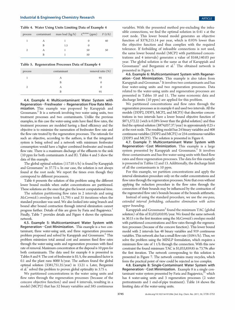
ð40ÞOne of the decisions that have to be made is regarding thevariable of that bilinear term that is being partitioned. For watermanagement problems, the bilinear terms generated by thesplitters are formed by the following variables: Outlet concentra-tion of the processes (water-using units and regenerationprocesses); and, flow rates. Thus, one must choose to partitionoutlet concentrations of processes, flow rates or both. The choicehas effect on the tightness of the lower bound, the increase innumber of binaries due to partitions/linearizations and theefficiency of the MILP formulation. Following Faria andBagajewicz,1 we show the number of variables that need to bepartitioned in each case, comparing partitioning of flow rates andpartitioning of concentrations (Table 1). Note that the numberof flow rate variables is usually higher than the number of outletconcentrations variables (only the highlighted ones are not).Faria and Bagajewicz1 discussed in detail the merits of each choice.

4. WATER MANAGEMENT RESULTS

We show now several examples that illustrate the effectivenessof the method. Examples 1-4 are multicomponent refineryexamples; the first and the second without regeneration pro-cesses and the third with regeneration units, all three solving forminimum freshwater. All these four examples do not require anyelimination procedure because they find the solution at the firstLB. Example 5 is added to compare our method’s performancewith that of Karuppiah and Grossmann.2 In this case, theelimination procedure requires more than one iteration, so weuse it to illustrate the performance of different options. Examples6 and 7 are added to illustrate the performance of the method



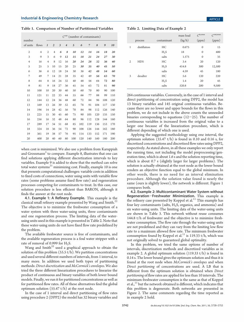
when cost is minimized. We also use a problem from Karuppiahand Grossmann2 to compare. Example 8, illustrates that one canfind solutions applying different discretization intervals to keyvariables. Example 9 is added to show that the method can solvetotal water systems21 minimizing cost. Finally, example 10 is onethat presents computational challenges: variable costs in additionto fixed costs of connections, water using units with variable flowrates (some problems assume fixed flow rate) and regenerationprocesses competing for contaminants to treat. In this case, oursolution procedure is less efficient than BARON, although itfinds the answer at the root node.4.1. Example 1: A Refinery Example. This example is the

classical small refinery example presented by Wang and Smith.22

The objective is to minimize the freshwater consumption of awater system with three water-using units, three contaminantsand one regeneration process. The limiting data of the water-using units used in this example is presented in Table 2. Note thatthese water-using units do not have fixed flow rate predefined bythe problem.The available freshwater source is free of contaminants, and

the available regeneration process is a foul water stripper with arate of removal of 0.999 for H2S.Wang and Smith22 used a graphical approach to obtain the

solution of this problem (55.5 t/h). We partition concentrationsand used several different numbers of intervals, from 1 interval, tomany more. In addition we used both types of partitioningmethods:Direct discretization andMcCormick’s envelopes. We alsotried the three different linearization procedures to linearize theproduct of continuous and binary variables of both lower boundmodels. Finally, we run it for partitioned concentrations as well asfor partitioned flow rates. All of these alternatives find the globaloptimum solution (55.47 t/h) at the root node.In the case of 1 interval and direct partitioning of flow rates

using procedure 2 (DPP2) the model has 32 binary variables and

264 continuous variables. Conversely, in the case of 1 interval anddirect partitioning of concentration using DPP2, the model has13 binary variables and 145 original continuous variables. Be-cause there are no lower and upper bounds for the flows in thisproblem, we do not include in the above counts the unneededbinaries corresponding to equations (12-25). The number ofcontinuous variables is increased from the original value to alarger one because of the linearization procedure, which isdifferent depending of which one is used.Applying the suggested methodology using one interval, the

optimum solution (55.47 t/h) is found in 0.10 and 0.16 s, fordiscretized concentrations and discretized flow rates usingDPP2,respectively. As stated above, in all these examples we only reportthe running time, not including the model preprocessing/gen-eration time, which is about 1.6 s and the solution reporting time,which is about 0.7 s (slightly larger for larger problems). Thesolution is actually obtained at the root node as the lower boundrenders an objective function equal to the global minimum. Inother words, there is no need for an interval eliminationprocedure. Although the solution value found is nearly thesame (ours is slightly lower), the network is different. Figure 1compares both.4.2. Example 2: Multicontaminant Water System without

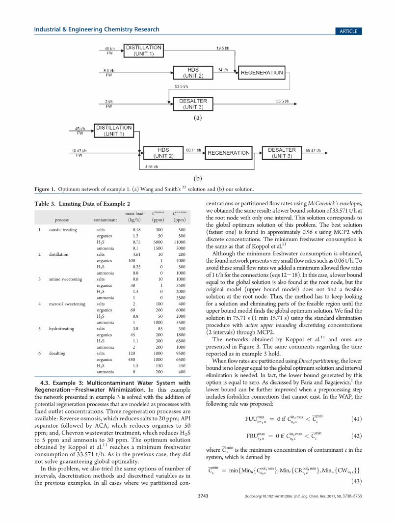
Regeneration-Freshwater Minimization. This example isthe refinery case presented by Koppol et al.11 This example hasfour key contaminants (salts, H2S, organics, and ammonia) andsix water-using units. The limiting data of the water-using unitsare shown in Table 3. This network without reuse consumes144.8 t/h of freshwater and the objective is to minimize fresh-water consumption. The flow rate through the water-using unitsare not predefined and they can vary from the limiting low flowrate to a maximum allowed flow rate. The minimum freshwaterconsumption found by Koppol et al.11 is 119.33 t/h, which wasnot originally solved to guaranteed global optimality.In this problem, we tried the same options of number of

intervals, discretization methods and discretized variables as inexample 2. A global optimum solution (119.33 t/h) is found in0.14 s. The lower bound gives the optimum solution and thus it isfound at the root node when McCormick’s envelopes and whenDirect partitioning of concentrations are used. A LB that isdifferent from the optimum solution is obtained when Directpartitioning of flow rates are applied for less than 10 intervals. Theminimum freshwater consumption is the same as that of Koppolet al.,11 but the network obtained is different, which indicates thatthis problem is degenerate. Both networks are presented inFigure 2. The same comments regarding the time reported asin example 2 hold.

Table 1. Comparison of Number of Partitioned Variables

Cout (number of contaminants)number

of units flows 1 2 3 4 5 6 7 8 9 10

2 4 2 4 6 8 10 12 14 16 18 20

3 9 3 6 9 12 15 18 21 24 27 30

4 16 4 8 12 16 20 24 28 32 36 40

5 25 5 10 15 20 25 30 35 40 45 50

6 36 6 12 18 24 30 36 42 48 54 60

7 49 7 14 21 28 35 42 49 56 63 70

8 64 8 16 24 32 40 48 56 64 72 80

9 81 9 18 27 36 45 54 63 72 81 90

10 100 10 20 30 40 50 60 70 80 90 100

11 121 11 22 33 44 55 66 77 88 99 110

12 144 12 24 36 48 60 72 84 96 108 120

13 169 13 26 39 52 65 78 91 104 117 130

14 196 14 28 42 56 70 84 98 112 126 140

15 225 15 30 45 60 75 90 105 120 135 150

16 256 16 32 48 64 80 96 112 128 144 160

17 289 17 34 51 68 85 102 119 136 153 170

18 324 18 36 54 72 90 108 126 144 162 180

19 361 19 38 57 76 95 114 133 152 171 190

20 400 20 40 60 80 100 120 140 160 180 200

Table 2. Limiting Data of Example 2

process contaminant

mass load

(kg/h)

Cin,max

(ppm)

Cout,max

(ppm)

1 distillation HC 0.675 0 15

H2S 18 0 400

salts 1.575 0 35

2 HDS HC 3.4 20 120

H2S 414.8 300 12,500

salts 4.59 45 180

3 desalter HC 5.6 120 220

H2S 1.4 20 45

salts 520.8 200 9,500



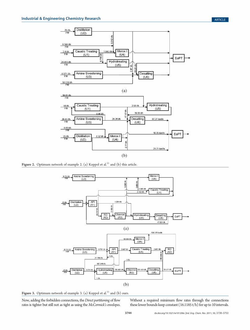
4.3. Example 3: Multicontaminant Water System withRegeneration-Freshwater Minimization. In this examplethe network presented in example 3 is solved with the addition ofpotential regeneration processes that are modeled as processes withfixed outlet concentrations. Three regeneration processes areavailable: Reverse osmosis, which reduces salts to 20 ppm; APIseparator followed by ACA, which reduces organics to 50ppm; and, Chevron wastewater treatment, which reduces H2Sto 5 ppm and ammonia to 30 ppm. The optimum solutionobtained by Koppol et al.11 reaches a minimum freshwaterconsumption of 33.571 t/h. As in the previous case, they didnot solve guaranteeing global optimality.In this problem, we also tried the same options of number of

intervals, discretization methods and discretized variables as inthe previous examples. In all cases where we partitioned con-

centrations or partitioned flow rates usingMcCormick’s envelopes,we obtained the same result: a lower bound solution of 33.571 t/h atthe root node with only one interval. This solution corresponds tothe global optimum solution of this problem. The best solution(fastest one) is found in approximately 0.56 s using MCP2 withdiscrete concentrations. The minimum freshwater consumption isthe same as that of Koppol et al.11

Although the minimum freshwater consumption is obtained,the found network presents very small flow rates such as 0.06 t/h. Toavoid these small flow rates we added aminimum allowed flow ratesof 1 t/h for the connections (eqs 12-18). In this case, a lower boundequal to the global solution is also found at the root node, but theoriginal model (upper bound model) does not find a feasiblesolution at the root node. Thus, the method has to keep lookingfor a solution and eliminating parts of the feasible region until theupper bound model finds the global optimum solution. We find thesolution in 75.71 s (1 min 15.71 s) using the standard eliminationprocedure with active upper bounding discretizing concentrations(2 intervals) through MCP2.The networks obtained by Koppol et al.11 and ours are

presented in Figure 3. The same comments regarding the timereported as in example 3 hold.When flow rates are partitioned usingDirect partitioning, the lower

bound is no longer equal to the global optimum solution and intervalelimination is needed. In fact, the lower bound generated by thisoption is equal to zero. As discussed by Faria and Bagajewicz,1 thelower bound can be further improved when a preprocessing stepincludes forbidden connections that cannot exist. In the WAP, thefollowing rule was proposed:

FUUmaxu�, u ¼ 0 if Cin, max

u, c < Cminc ð41Þ

FRUmaxr, u ¼ 0 if Cin, max

u, c < Cminc ð42Þ

where Ccmin is the minimum concentration of contaminant c in the

system, which is defined by

Cminc ¼ minfMinufCout, min

u, c g, MinrfCRout,minr, c g, MinwfCWw, cgg

ð43Þ

Figure 1. Optimum network of example 1. (a) Wang and Smith's 22 solution and (b) our solution.

Table 3. Limiting Data of Example 2

process contaminantmass load(kg/h)

Cin,max

(ppm)Cout,max

(ppm)

1 caustic treating salts 0.18 300 500organics 1.2 50 500H2S 0.75 5000 11000ammonia 0.1 1500 3000

2 distillation salts 3.61 10 200organics 100 1 4000H2S 0.25 0 500ammonia 0.8 0 1000

3 amine sweetening salts 0.6 10 1000organics 30 1 3500H2S 1.5 0 2000ammonia 1 0 3500

4 merox-I sweetening salts 2 100 400organics 60 200 6000H2S 0.8 50 2000ammonia 1 1000 3500

5 hydrotreating salts 3.8 85 350organics 45 200 1800H2S 1.1 300 6500ammonia 2 200 1000

6 desalting salts 120 1000 9500organics 480 1000 6500H2S 1.5 150 450ammonia 0 200 400



Now, adding the forbidden connections, theDirect partitioning of flowrates is tighter but still not as tight as using theMcCormick’s envelopes.

Without a required minimum flow rates through the connectionsthese lower bounds keep constant (16.1185 t/h) for up to 10 intervals.

Figure 2. Optimum network of example 2. (a) Koppol et al.11 and (b) this article.

Figure 3. Optimum network of example 3. (a) Koppol et al.11 and (b) ours.



4.4. Example 4: Multicontaminant Water System withRegeneration-Freshwaterþ Regeneration Flow Rate Mini-mization. This example was proposed by Karuppiah andGrossmann.2 It is a network involving two water using units, twotreatment processes and two contaminants. Unlike the previousexamples, in this case the water-using units have fixed flow rates, thetreatment processes are modeled having a fixed efficiency and theobjective is to minimize the summation of freshwater flow rate andthe flow rate treated by the regeneration processes. The rationale forsuch an objective, according to the authors, is that the integratedsystem is being solved and a network with minimum freshwaterconsumption would have a higher combined freshwater and treatedflow rate. There is a maximum discharge of the effluents to the sink(10 ppm for both contaminants A and B). Tables 4 and 5 show thedata of this example.The global optimal solution (117.05 t/h) is found by Karuppiah

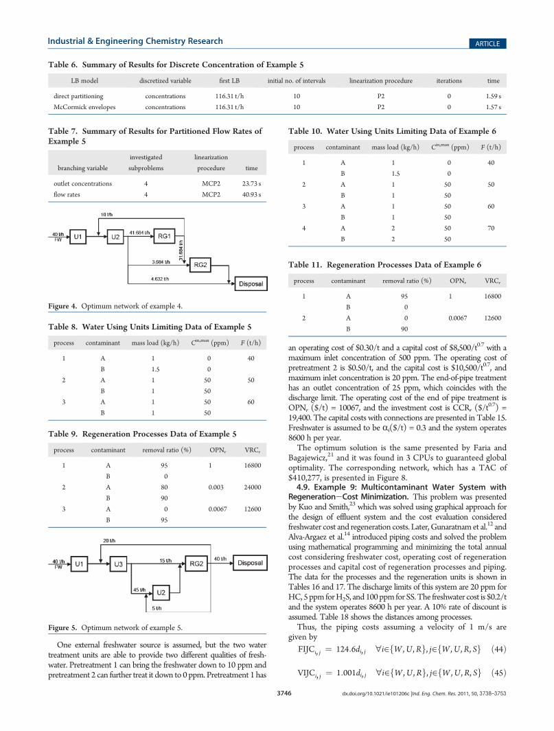
and Grossmann2 in 37.72 s. In our case, the solution is not alwaysfound at the root node. We report the times even though theycorrespond to different processors.Table 6 presents the solution of this problem using the different

lower bound models when outlet concentrations are partitioned.These solutions are the ones that give the lowest computational time.The solution partitioning flow rates in 2 intervals and using

McCormick’s envelopes took 11,795 s and 35 iterations when thestandard procedure was used. We also looked into using branch andbound after bound contraction through interval elimination cannotprogress further. Details of this are given by Faria and Bagajewicz.1

Finally, Table 7 provides details and Figure 4 shows the optimumnetwork.4.5. Example 5: Multicontaminant Water System with

Regeneration-Cost Minimization. This example is a two con-taminant, three water-using unit, and three regeneration processesproblem proposed and solved by Karuppiah and Grossmann.2 Thisproblem minimizes total annual cost and assumes fixed flow ratesthrough the water-using units and regeneration processes with fixedrate of removal.Maximumconcentration at the disposal is 10 ppm forboth contaminants. The data used for example 6 is presented inTables 8 and 9. The cost of freshwater is $1/t, the annualized factor is0.1 and the plant runs 8000 h/year. The authors found the globaloptimal solution ($381,751.35/year) in 13.21 s. Later, Bergaminiet al.7 solved this problem to proven global optimality in 3.75 s.We partitioned concentrations in the water using units and

flow rates through the regeneration processes (because of theconcave objective function) and used 4 intervals, resulting in amodel (MCP2) that has 52 binary variables and 585 continuous

variables. With the presented method pre-excluding the infea-sible connections, we find the optimal solution in 0.41 s at theroot node. This lower bound model generates an objectivefunction of $378,215.14 per year, which is 0.93% lower thanthe objective function and thus complies with the requiredtolerance. If forbidding of infeasible connections is not used,the same lower bound model (MCP2 with partitioned concen-trations and 4 intervals) generates a value of $168,140.03 peryear. The global solution is the same as that of Karuppiah andGrossmann2 and Bergamini et al.7 The obtained network ispresented in Figure 5.4.6. Example 6: Multicontaminant System with Regener-

ation-Cost Minimization. This example is also taken fromKaruppiah and Grossman.2 It involves two contaminants and hasfour water-using units and two regeneration processes. Datarelated to the water-using units and regeneration processes arepresented in Tables 10 and 11. The same economic data anddischarge limits (10 ppm) are applied for this problem.We partitioned concentrations and flow rates through the

regeneration processes as in example 6 and used two intervals. All themodels (DDP2, DDP3, MCP2, and MCP3) that discretize concen-trations in two intervals have a lower bound objective function of$871,572.22 (wich is 0.28% lower than the global solution) and thusfind the optimal solution ($874,057.37/year) in approximately 0.25 sat the root node. The resultingmodel has 24 binary variables and 408continuous variables (DDP2andMCP2) or 254 continuous variables(DDP3 and MCP3). The solution is presented in Figure 6.4.7. Example 7: Multicontaminant Water System with

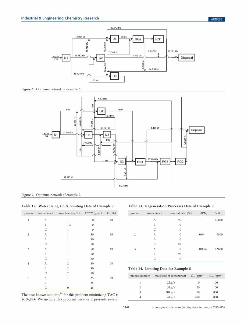
Regeneration-Cost Minimization. This example is a largesystem presented by Karuppiah and Grossmann.2 It involvesthree contaminants and has five water-using units with fixed flowrates and three regeneration processes. The data for this exampleis presented in Tables 12 and 13. Additionally, the discharge limitof all the contaminants is 10 ppm.For this example, we partition concentrations and apply the

interval elimination procedure only on the outlet concentrations andflow rates through the regeneration processes.Note that evenwithoutapplying the reduction procedure in the flow rates through theconnection of their bounds may be influenced by the contraction ofthe regenerated flow rate’s bounds because of the bounds arithmetic.Instead of using the standard procedure, we use the one-pass,

extended interval forbidding, exhaustive elimination with activeupper bounding.Karuppiah and Grossmann2 found the minimum TAC (global

solution) of this of $1,033,810.95/year. We found the same networkin 30.15 s in the first iteration using theMcCormick’s envelopesmodelwith partitioned concentrations and flow rates through the regenera-tion processes (because of the concave function). This lower boundmodel with 2 intervals has 48 binary variables and 919 continuousvariables. This network also has a small flow rate (0.04 t/h). Thus, wesolve the problem using the MINLP formulation, which requires aminimum flow rate of 1 t/h through the connection. With this newconstraint the found minimum TAC is $1,033,859.85 in 73.79s afterthe first iteration. The network corresponding to this solution ispresented in Figure 7. The network contains many recycles, whichform the practical point of view could be rejected as too complex.4.8. Example 8: Single-Contaminant Water System with

Regeneration-Cost Minimization. Example 8 is a single con-taminant water system presented by Faria and Bagajewicz,21 whichhas 4 water-using units and 3 regeneration processes (2 waterpretreatments and 1 end-of-pipe treatment). Table 14 shows thelimiting data of the water-using units.

Table 4. Water Using Units Limiting Data of Example 4

process contaminant mass load (kg/h) Cin,max (ppm) F (t/h)

1 A 1 0 40

B 1.5 0

2 A 1 50 50

B 1 50

Table 5. Regeneration Processes Data of Example 4

process contaminant removal ratio (%)

1 A 95

B 0

2 A 0

B 95



One external freshwater source is assumed, but the two watertreatment units are able to provide two different qualities of fresh-water. Pretreatment 1 can bring the freshwater down to 10 ppm andpretreatment 2 can further treat it down to 0 ppm. Pretreatment 1 has

an operating cost of $0.30/t and a capital cost of $8,500/t0.7 with amaximum inlet concentration of 500 ppm. The operating cost ofpretreatment 2 is $0.50/t, and the capital cost is $10,500/t0.7, andmaximum inlet concentration is 20 ppm. The end-of-pipe treatmenthas an outlet concentration of 25 ppm, which coincides with thedischarge limit. The operating cost of the end of pipe treatment isOPNr ($/t) = 10067, and the investment cost is CCRr ($/t

0.7) =19,400. The capital costs with connections are presented in Table 15.Freshwater is assumed to be Ri($/t) = 0.3 and the system operates8600 h per year.The optimum solution is the same presented by Faria and

Bagajewicz,21 and it was found in 3 CPUs to guaranteed globaloptimality. The corresponding network, which has a TAC of$410,277, is presented in Figure 8.4.9. Example 9: Multicontaminant Water System with

Regeneration-Cost Minimization. This problem was presentedby Kuo and Smith,23 which was solved using graphical approach forthe design of effluent system and the cost evaluation consideredfreshwater cost and regeneration costs. Later, Gunaratnamet al.12 andAlva-Argaez et al.14 introduced piping costs and solved the problemusing mathematical programming and minimizing the total annualcost considering freshwater cost, operating cost of regenerationprocesses and capital cost of regeneration processes and piping.The data for the processes and the regeneration units is shown inTables 16 and 17. The discharge limits of this system are 20 ppm forHC, 5ppm forH2S, and100ppm for SS.The freshwater cost is $0.2/tand the system operates 8600 h per year. A 10% rate of discount isassumed. Table 18 shows the distances among processes.Thus, the piping costs assuming a velocity of 1 m/s are

given byFIJCi, j ¼ 124:6di, j "i∈fW ,U ,Rg, j∈fW ,U ,R, Sg ð44Þ

VIJCi, j ¼ 1:001di, j "i∈fW ,U ,Rg, j∈fW ,U ,R, Sg ð45Þ

Table 6. Summary of Results for Discrete Concentration of Example 5

LB model discretized variable first LB initial no. of intervals linearization procedure iterations time

direct partitioning concentrations 116.31 t/h 10 P2 0 1.59 s

McCormick envelopes concentrations 116.31 t/h 10 P2 0 1.57 s



1 A 1 0 40

B 1.5 0

2 A 1 50 50

B 1 50

3 A 1 50 60

B 1 50


process contaminant removal ratio (%) OPNr VRCr

1 A 95 1 16800

B 0

2 A 80 0.003 24000

B 90

3 A 0 0.0067 12600

B 95



1 A 1 0 40

B 1.5 0

2 A 1 50 50

B 1 50

3 A 1 50 60

B 1 50

4 A 2 50 70

B 2 50



1 A 95 1 16800

B 0

2 A 0 0.0067 12600

B 90

Table 7. Summary of Results for Partitioned Flow Rates ofExample 5

branching variable

investigated

subproblems

linearization

procedure time

outlet concentrations 4 MCP2 23.73 s

flow rates 4 MCP2 40.93 s

Figure 4. Optimum network of example 4.




The best known solution14 for this problem minimizing TAC is$616,824. We include this problem because it presents several





1 A 95 1 16800

B 0

C 0

2 A 0 0.04 9500

B 0

C 95

3 A 0 0.0067 12600

B 95

C 0

Table 14. Limiting Data for Example 8

process number mass load of contaminant Cin (ppm) Cout (ppm)

1 2 kg/h 0 100

2 5 kg/h 20 100

3 30 kg/h 50 800

4 4 kg/h 400 800



1 A 1 0 40

B 1.5 0

C 1 0

2 A 1 50 50

B 1 50

C 1 50

3 A 1 50 60

B 1 50

C 1 50

4 A 2 50 70

B 2 50

C 2 50

5 A 1 25 80

B 1 25

C 0 25



challenges: fixed and variable cost for connection and minimumallowed flow rates through the connections, which makes it a

MINLP problem; water-using units with variable flow rates; and,competing regeneration processes (more than one process is ableto treat the same contaminant). We assume the minimum flowrate through connection and units is 5 t/h and the maximum is200 t/h.BARON solves this problem to global optimality (1% gap) in

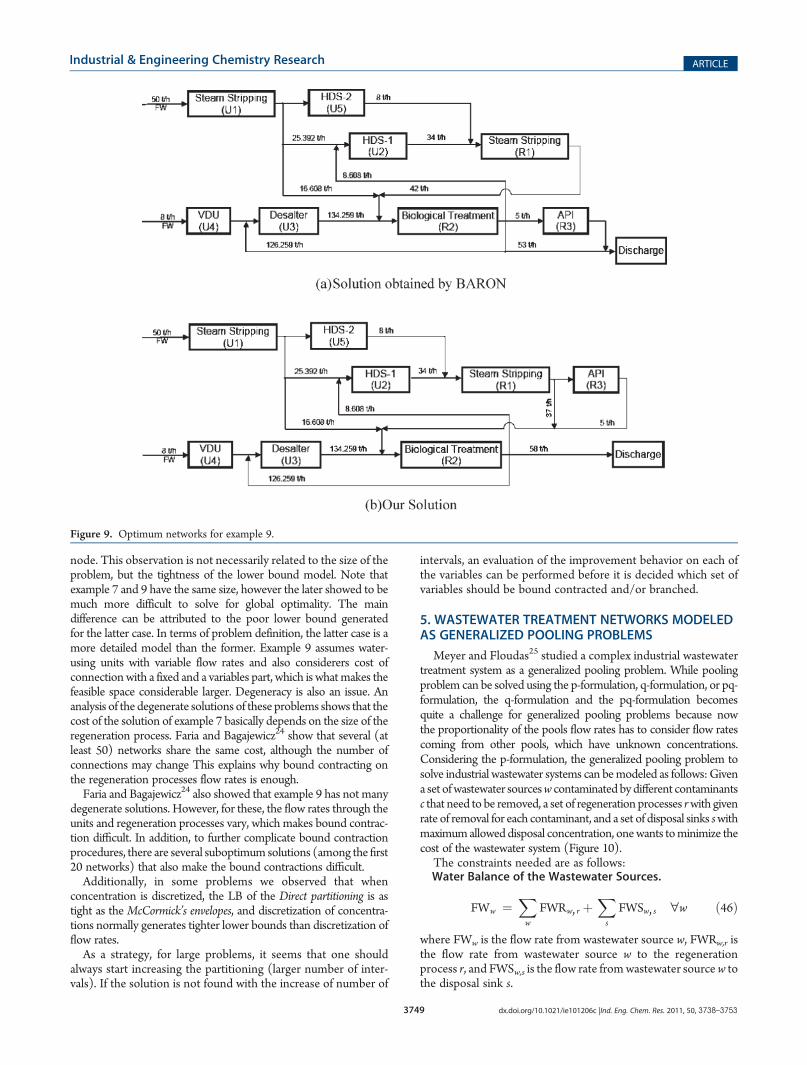
25513 s (7 h, 5 m, 13 s), with the minimum TAC of $574,155.Using the GO method with elimination on discretized variablepresented in this section, the lowest time achieved to guaranteethe 1% tolerance solution was 25293 CPUs (7 h 1 m 33 s).Incidentally, our wall clock time is 57960 CPUs (16 h 6 m). It ishard to make a meaningful comparison because our code isimplemented in GAMS and includes a preprocessing time eachtime a LB is solved, whereas BARON may skip these steps. Ourmethod analyzes 62 sub problems or passes through the elimina-tion procedure (steps 1 through 7). This procedure used MCP2with 2 intervals on concentrations and 5 on all flows (units andregeneration processes). Although the presented method takeslonger than BARON to find the GO solution, it finds it afterbound contraction is performed at the root node. The optimumnetwork found has a TAC of $578,183, which is higher than andcomparable to the one obtained by BARON, but well within the1% gap. As one can observe in Figure 9, the solutions are similar.4.10. Comparative Analysis. It seems that using the larger

number of intervals possible reduces the number of iterationswhen the problems are relatively small, which many times do notneed any iteration because the solution can be found at the root

Table 15. Capital Costs of the Connections

unit 1 unit 2 unit 3 unit 4 WPT 1 WPT 2 end of pipe treatment

FW $39,000 $76,000 $47,000 $92,000

unit 1 $150,000 $110,000 $45,000 $39,000 $39,000 $83,000

unit 2 $50,000 $134,000 $40,000 $76,000 $76,000 $102,500

unit 3 $180,000 $35,000 $42,000 $47,000 $47,000 $98,000

unit 4 $163,000 $130,000 $90,000 $92,000 $92,000 $124,000

WPT 1 $39,000 $76,000 $47,000 $92,000

WPT 2 $39,000 $76,000 $47,000 $92,000

EoPT $83,000 $102,500 $98,000 $124,000


Table 16. Water-Using Units Limiting Data of Example 9

process contaminant

mass

load (kg/h)

Cin,max

(ppm)

Cout,max

(ppm)

1 steam stripping HC 0.75 0 15

H2S 20 0 400

SS 1.75 0 35

2 HDS-1 HC 3.4 20 120

H2S 414.8 300 12500

SS 4.59 45 180

3 desalter HC 5.6 120 220

H2S 1.4 20 45

SS 520.8 200 9500

4 VDU HC 0.16 0 20

H2S 0.48 0 60

SS 0.16 0 20

5 HDS-2 HC 0.8 50 150

H2S 60.8 400 8000

SS 0.48 60 120


process contaminant

removal

ratio (%) OPNr VRCr

1 steam stripping HC 0 1 16800

H2S 99.9

SS 0

2 biological treatment HC 70 0.0067 12600

H2S 90

SS 98

3 API separator HC 95 0 4,800

H2S 0

SS 50

Table 18. Distances for Example 9

di,j WU 1 WU 2 WU 3 WU 4 WU 5 RG 1 RG 2 RG 3 discharge

FW 30 25 70 50 90 200 500 600 2000WU 1 0 30 80 150 400 90 150 200 1200WU 2 30 0 60 100 165 100 150 150 1000WU 3 80 60 0 50 75 120 90 350 800WU 4 150 100 50 0 150 250 170 400 650WU 5 400 165 75 150 0 300 120 200 300RG 1 90 100 120 250 300 0 125 80 250RG 2 150 150 90 170 120 125 0 35 100RG 3 200 150 350 400 200 80 35 0 100



node. This observation is not necessarily related to the size of theproblem, but the tightness of the lower bound model. Note thatexample 7 and 9 have the same size, however the later showed to bemuch more difficult to solve for global optimality. The maindifference can be attributed to the poor lower bound generatedfor the latter case. In terms of problem definition, the latter case is amore detailed model than the former. Example 9 assumes water-using units with variable flow rates and also considerers cost ofconnectionwith a fixed and a variables part, which is whatmakes thefeasible space considerable larger. Degeneracy is also an issue. Ananalysis of the degenerate solutions of these problems shows that thecost of the solution of example 7 basically depends on the size of theregeneration process. Faria and Bagajewicz24 show that several (atleast 50) networks share the same cost, although the number ofconnections may change This explains why bound contracting onthe regeneration processes flow rates is enough.Faria and Bagajewicz24 also showed that example 9 has not many

degenerate solutions. However, for these, the flow rates through theunits and regeneration processes vary, which makes bound contrac-tion difficult. In addition, to further complicate bound contractionprocedures, there are several suboptimum solutions (among thefirst20 networks) that also make the bound contractions difficult.Additionally, in some problems we observed that when

concentration is discretized, the LB of the Direct partitioning is astight as the McCormick’s envelopes, and discretization of concentra-tions normally generates tighter lower bounds than discretization offlow rates.As a strategy, for large problems, it seems that one should

always start increasing the partitioning (larger number of inter-vals). If the solution is not found with the increase of number of

intervals, an evaluation of the improvement behavior on each ofthe variables can be performed before it is decided which set ofvariables should be bound contracted and/or branched.

5. WASTEWATER TREATMENT NETWORKS MODELEDAS GENERALIZED POOLING PROBLEMS

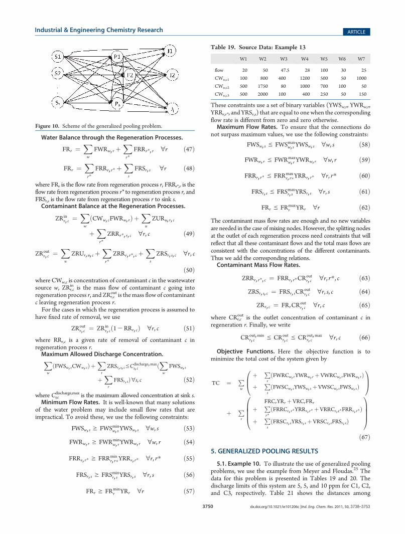
Meyer and Floudas25 studied a complex industrial wastewatertreatment system as a generalized pooling problem. While poolingproblem can be solved using the p-formulation, q-formulation, or pq-formulation, the q-formulation and the pq-formulation becomesquite a challenge for generalized pooling problems because nowthe proportionality of the pools flow rates has to consider flow ratescoming from other pools, which have unknown concentrations.Considering the p-formulation, the generalized pooling problem tosolve industrial wastewater systems can bemodeled as follows:Givena set ofwastewater sourcesw contaminatedbydifferent contaminantsc that need to be removed, a set of regeneration processes rwith givenrate of removal for each contaminant, and a set of disposal sinks swithmaximumalloweddisposal concentration, onewants tominimize thecost of the wastewater system (Figure 10).

The constraints needed are as follows:Water Balance of the Wastewater Sources.

FWw ¼Xw

FWRw, r þXs

FWSw, s "w ð46Þ

where FWw is the flow rate from wastewater source w, FWRw,r isthe flow rate from wastewater source w to the regenerationprocess r, and FWSw,s is the flow rate fromwastewater sourcew tothe disposal sink s.

Figure 9. Optimum networks for example 9.



Water Balance through the Regeneration Processes.

FRr ¼Xw

FWRw, r þXr�

FRRr�, r "r ð47Þ

FRr ¼Xr�

FRRr, r� þXs

FRSr, s "r ð48Þ

where FRr is the flow rate from regeneration process r, FRRr*,r is theflow rate from regeneration process r* to regeneration process r, andFRSr,s is the flow rate from regeneration process r to sink s.Contaminant Balance at the Regeneration Processes.

ZRinr, c ¼

Xw

ðCWw, cFWRw, rÞþXu

ZURu, r, c

þXr�

ZRRr�, r, c "r, c ð49Þ

ZRoutr, c ¼

Xu

ZRUr, u, c þXr�

ZRRr, r�, c þXs

ZRSr, s, c "r, c

ð50Þwhere CWw,c is concentration of contaminant c in the wastewatersource w, ZRr,c

in is the mass flow of contaminant c going intoregeneration process r, and ZRr,c

out is themass flow of contaminantc leaving regeneration process r.For the cases in which the regeneration process is assumed to

have fixed rate of removal, we use

ZRoutr, c ¼ ZRin

r, cð1-RRr, cÞ "r, c ð51Þwhere RRr,c is a given rate of removal of contaminant c inregeneration process r.Maximum Allowed Discharge Concentration.X

w

ðFWSw, sCWw, cÞþXr

ZRSr, s, ceCdischarge, maxs, c ð

Xw

FWSw, s

þXr

FRSr, sÞ"s, c ð52Þ

where Cs,cdischarge,max is the maximum allowed concentration at sink s.

Minimum Flow Rates. It is well-known that many solutionsof the water problem may include small flow rates that areimpractical. To avoid these, we use the following constraints:

FWSw, s g FWSminw, sYWSw, s "w, s ð53ÞFWRw, r g FWRmin

w, rYWRw, r "w, r ð54Þ

FRRr, r� g FRRminr, r�YRRr, r� "r, r� ð55Þ

FRSr, s g FRSminr, s YRSr, s "r, s ð56Þ

FRr g FRminr YRr "r ð57Þ

These constraints use a set of binary variables (YWSw,r, YWRw,r,YRRr,r*, and YRSr,s) that are equal to one when the correspondingflow rate is different from zero and zero otherwise.Maximum Flow Rates. To ensure that the connections do

not surpass maximum values, we use the following constraints:

FWSw, s e FWSmaxw, s YWSw, s "w, s ð58Þ

FWRw, r e FWRmaxw, r YWRw, r "w, r ð59Þ

FRRr, r� e FRRmaxr, r�YRRr, r� "r, r� ð60Þ

FRSr, s e FRSmaxr, s YRSr, s "r, s ð61Þ

FRr e FRmaxr YRr "r ð62Þ

The contaminant mass flow rates are enough and no new variablesare needed in the case of mixing nodes. However, the splitting nodesat the outlet of each regeneration process need constraints that willreflect that all these contaminant flows and the total mass flows areconsistent with the concentrations of the different contaminants.Thus we add the corresponding relations.Contaminant Mass Flow Rates.

ZRRr, r�, c ¼ FRRr, r�CRoutr, c "r, r�, c ð63Þ

ZRSr, s, c ¼ FRSr, sCRoutr, c "r, s, c ð64Þ

ZRr, c ¼ FRrCRoutr, c "r, c ð65Þ

where CRr,cout is the outlet concentration of contaminant c in

regeneration r. Finally, we write

CRout, minr, c e CRout

r, c e CRout, maxr, c "r, c ð66Þ

Objective Functions. Here the objective function is tominimize the total cost of the system given by

TC ¼ Pw

þ PrðFWRCw, rYWRw, r þVWRCw, rFWRw, rÞ

þ PsðFWSCw, sYWSw, s þVWSCw, sFWSw, sÞ

0B@

1CA

þ Pr

FRCrYRr þVRCrFRr

þ Pr�ðFRRCr, r�YRRr, r� þVRRCr, r�FRRr, r�Þ

þ PsðFRSCr, sYRSr, s þVRSCr, sFRSr, sÞ

0BBBB@

1CCCCA

ð67Þ5. GENERALIZED POOLING RESULTS

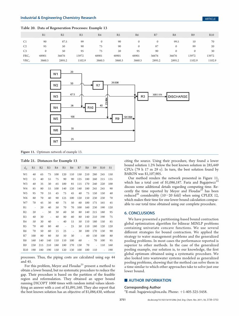
5.1. Example 10. To illustrate the use of generalized poolingproblems, we use the example from Meyer and Floudas.25 Thedata for this problem is presented in Tables 19 and 20. Thedischarge limits of this system are 5, 5, and 10 ppm for C1, C2,and C3, respectively. Table 21 shows the distances among

Figure 10. Scheme of the generalized pooling problem.

Table 19. Source Data: Example 13

W1 W2 W3 W4 W5 W6 W7

flow 20 50 47.5 28 100 30 25

CWw,c1 100 800 400 1200 500 50 1000

CWw,c2 500 1750 80 1000 700 100 50

CWw,c3 500 2000 100 400 250 50 150



processes. Thus, the piping costs are calculated using eqs 44and 45.For this problem, Meyer and Floudas25 present a method to

obtain a lower bound, but no systematic procedure to reduce thegap. Their procedure is based on the partition of the feasibleregion and reformulation. They obtained an upper boundrunning DICOPT 1000 times with random initial values identi-fying an answer with a cost of $1,091,160. They also report thatthe best known solution has an objective of $1,086,430, without

citing the source. Using their procedure, they found a lowerbound solution 1.2% below the best known solution in 285,449CPUs (79 h 17 m 29 s). In turn, the best solution found byBARON was $1,107,905.Our method renders the network presented in Figure 11,

which has a total cost of $1,086,187. Faria and Bagajeiwcz24

discuss some additional details regarding computing time. Re-cently the time reported by Meyer and Floudas25 has beenreduced26 considerably (10-20 fold) when using CPLEX 12,which makes their time for one lower bound calculation compar-able to our total time obtained using our complete procedure.

6. CONCLUSIONS

We have presented a partitioning-based bound contractionglobal optimization algorithm for bilinear MINLP problemscontaining univariate concave functions. We use severaldifferent strategies for bound contraction. We applied thestrategy to water management problems and the generalizedpooling problems. In most cases the performance reported issuperior to other methods. In the case of the generalizedpooling example, our solution is, to our knowledge, the firstglobal optimum obtained using a systematic procedure. Wealso looked into wastewater systems modeled as generalizedpooling problems, showing that the method can solve them ina time similar to which other approaches take to solve just onelower bound.

’AUTHOR INFORMATION

Corresponding Author*E-mail: [email protected]. Phone: þ1-405-325-5458.

Table 20. Data of Regeneration Processes: Example 13

R1 R2 R3 R4 R5 R6 R7 R8 R9 R10

C1 90 87.5 99 0 90 0 0 99.5 10 70

C2 95 50 90 75 90 0 87 0 99 20

C3 0 50 95 75 20 95 90 0 0 30

FRCr 48901 36676 13972 48901 48901 48901 36676 36676 13972 13972

VRCr 3860.3 2895.2 1102.9 3860.3 3860.3 3860.3 2895.2 2895.2 1102.9 1102.9


Table 21. Distances for Example 13

di,j R1 R2 R3 R4 R5 R6 R7 R8 R9 R10 S1

W1 40 65 75 100 120 110 150 210 280 245 150

W2 15 40 55 75 90 90 125 180 260 215 135

W3 40 35 30 65 100 85 115 170 240 220 100

W4 85 80 55 100 140 120 140 180 245 245 90

W5 95 70 55 45 75 45 40 75 150 150 40

W6 80 70 40 90 125 100 120 150 230 230 70

W7 70 45 30 40 75 50 60 100 175 165 45

R1 - 20 40 50 70 70 100 160 230 190 120

R2 20 - 30 30 60 50 80 140 215 180 95

R3 40 30 - 40 80 60 80 140 210 190 75

R4 50 30 40 - 40 15 50 110 180 150 85

R5 70 60 80 40 - 25 50 110 180 120 120

R6 70 50 60 15 25 - 30 100 170 130 90

R7 100 80 80 50 50 30 - 60 130 100 80

R8 160 140 140 110 110 100 60 - 70 100 95

R9 230 215 210 180 180 170 130 70 - 110 160

R10 190 180 190 150 120 130 100 100 110 - 190



’ACKNOWLEDGMENT

D�ebora Faria acknowledges support from the CAPES/Fulb-right Program (Brazil).

’NOMENCLATUREFWUw,u = flow rate from freshwater source w to the unit uFUUu*,u = flow rates between units u* and uFRUr,u = flow rate from regeneration process r to unit uFUSu,s = flow rate from unit u to sink sFURu*,r = flow rate from unit u to regeneration process rFWRw,r = flow rate from freshwater source w to the regeneration

process rFRRr*,r = flow rate from regeneration process r* to regeneration

process rFRSr,s = flow rate from regeneration process r to sink sCWw,c = Concentration of contaminant c in the freshwater sourcewΔMu,c = mass load of contaminant c extracted in unit uZUUu*,u,c =mass flow of contaminant c in the stream leaving unit u*

and going to unit uZRUr,u,c = mass flow of contaminant c in the stream leaving

regeneration process r and going to unit uZUSu,s,c = mass flow of contaminant c in the stream leaving unit u

and going to sink sZURu,r,c = mass flow of contaminant c in the stream leaving unit u

and going to regeneration process rCu,cin,max = maximum allowed concentration of contaminant c at the

inlet of unit uCu,cout,max = maximum allowed concentration of contaminant c at the

outlet of unit uZRr,c

in =mass flow of contaminant c going into regeneration process rZRr,c

out = mass flow of contaminant c leaving regeneration process rCRFr,c

out = outlet concentration of contaminant c in regenerationprocess r

XCRr,c = binary parameter that indicates if contaminant c istreated by regeneration process r

RRr,c = rate of removal of contaminant c in regeneration process rCAPr = capacity of regeneration process rCs,cdischarge,max = maximum allowed concentration at sink s

YWUw,u = binary variable to define the existence of a connectionbetween freshwater source w and unit u

YUUu,u* = binary variable to define the existence of a connectionbetween unit u and unit u*

YUSu,s = binary variable to define the existence of a connectionbetween unit u and sink s

YURu,r = binary variable to define the existence of a connectionbetween unit u and regeneration process r

YRUr,u = binary variable to define the existence of a connectionbetween regeneration process r and unit u

YRRr,r* = binary variable to define the existence of a connec-tion between regeneration process r and regenerationprocess r*

YRSr,s = binary variable to define the existence of a connectionbetween regeneration process r and sink s

Cu,cout = outlet concentration of contaminant c in unit u

CRr,cout = outlet concentration of the not treated contaminant c in

regeneration rFW = freshwater consumptionFWUw,u = freshwater from source w consumed by unit uFWRw,r = freshwater from source w consumed by regeneration

process r

TAC = the total annual costOPNr = operational cost of the regeneration processesOP = hours of operation per yearaf = annualization factorN = number of years of depreciationCCRr = capital cost coefficient of the regeneration processesFCI = fixed capital of investmentFWUCw,u = fixed capital cost of the connection between freshwater

source w and unit uFWRCw,r = fixed capital cost of the connection between freshwater

source w and regeneration process rFWSCw,s = fixed capital cost of the connection between freshwater

source w and sink sFUUCu,u* = fixed capital cost of the connection between freshwater

unit u and unit u*FURCu,r = fixed capital cost of the connection between freshwater

unit u and regeneration process rFUSCu,s = fixed capital cost of the connection between freshwater

unit u and sink sFRUCr,u= fixed capital cost of the connection between regeneration

process r and freshwater unit uFRRCr,r* = fixed capital cost of the connection between regeneration

process r and regeneration process r*FRSCr,s = fixed capital cost of the connection between regeneration

process r and regeneration process r*FRCr = fixed capital cost of regeneration process rVWUCw,u = coefficient of the variable capital cost of the connection

between freshwater source w and unit uVWRCw,r = coefficient of the variable capital cost of the connection

between freshwater sourcew and regeneration process rVWSCw,s = coefficient of the variable capital cost of the connection

between freshwater source w and sink sVUUCu,u* = coefficient of the variable capital cost of the connection

between freshwater unit u and unit u*VURCu,r = coefficient of the variable capital cost of the connection

between freshwater unit u and regeneration process rVUSCu,s = coefficient of the variable capital cost of the connection

between freshwater unit u and sink sVRUCr,u = coefficient of the variable capital cost of the connection

between regeneration process r and freshwater unit uVRRCr,r* = coefficient of the variable capital cost of the connec-

tion between regeneration process r and regenerationprocess r*

VRSCr,s = coefficient of the variable capital cost of the connectionbetween regeneration process r and regeneration process r*

VRCr = coefficient of the variable capital cost of regeneration process rdi,j = distance between two processesFWw = flow rate from wastewater source wFRr = flow rate from regeneration process rTC = total cost

’REFERENCES

(1) Faria, D.; Bagajewicz, M. A new approach for global optimizationof a class of MINLP problems with applications to water managementand pooling problems. AIChE J.

(2) Karuppiah, R.; Grossmann, I. E. Global optimization for thesynthesis of integrated water systems in chemical processes. Comput.Chem. Eng. 2006, 30, 650–673.

(3) McCormick, G. P. Computability of global solutions to factor-able nonconvex programs. Convex underestimating problems. Math.Program. 1976, 10 (1), 147–175.



(4) Zamora, J. M.; Grossmann, I. E. A branch and contract algorithmfor problems with concave univariate, bilinear and linear fractionalterms. J. Global Optim. 1999, 14, 217–249.(5) Karuppiah, R.; Grossmann, I. E. Global optimization of multi-

scenario mixed integer nonlinear programming models arising in thesynthesis of integrated water networks under uncertainty.Comput.-AidedChem. Eng. 2006, 21 (2), 1747–1752.(6) Bergamini, M. L.; Aguirre, P.; Grossmann, I. Logic based outer

approximation for global optimization of synthesis of process networks.Comput. Chem. Eng. 2005, 29, 1914.(7) Bergamini, M. L.; Grossmann, I.; Scenna, N.; Aguirre, P.

An improved piecewise outer-approximation algorithm for the globaloptimization of MINLP models involving concave and bilinear terms.Comput. Chem. Eng. 2008, 32, 477–493.(8) Padberg, M. Approximating separable nonlinear functions via

mixed zero-one programs. Oper. Res. Lett. 2000, 27, 1–5.(9) Meyer, C. A.; Floudas, C. A. Global optimization of a combina-

torially complex generalized pooling problem. AIChE J. 2006, 52 (3),1027–1037.(10) Savelski, M.; Bagajewicz, M. On the use of linear models for the

design of water utilization systems in refineries and process plants.Chem.Eng. Res. Des. 2001, 79, 600–610.(11) Koppol, A. P. R.; Bagajewicz, J. M.; Dericks, B. J.; Savelski, M. J.

On zero water discharge solutions in process industry. Adv. Environ. Res.2003, 8, 151–171.(12) Gunaratnam, M.; Alva-Argaez, A.; Kokosis, A.; Kim, J. K.;

Smith, R. Automated design of total water systems. Ind. Eng. Chem.Res. 2005, 44, 588–599.(13) Hallale, N.; Fraser, D. M. Capital cost targets for mass exchange

networks. A special case: Water minimization. Chem. Eng. Sci. 1998, 53(2), 293–313.(14) Alva-Argaez, A.; Kokossis, A. C.; Smith, R. A conceptual

decomposition of MINLPmodels for the design of water-using systems.Int. J. Environ. Pollut. 2007, 29, 177–205.(15) Faria, D. C.; Bagajewicz, M. J. Retrofit of water networks in

process plants. Proceedings of the XXII Interamerican Congress of ChemicalEngineering, Buenos Aires, Argentina; 2006.(16) Lim, S. R.; Park, D.; Lee, D. S.; Park, J. M. Economic evaluation

of water network system through the net present value method based oncost and benefits estimations. Ind. Eng. Chem. Res. 2006, 45, 7710–7718.(17) Lim, S. R.; Park, D.; Park, J. M. Synthesis of an economically

friendly water system by maximizing net present value. Ind. Eng. Chem.Res. 2007, 46, 6936–6943.(18) Wan Alwi, S. R.; Manan, Z. A. SHARPS: A new cost-screening

technique to attain cost-effective minimum water network. AIChE J.2006, 52, 3981–3988.(19) Wan Alwi, S. R.; Manan, Z. A.; Samingin, M. H.; Misran, N.

A holistic framework for design of cost-effective minimum water utiliza-tion network. J. Environ. Manage. 2007.(20) Faria, D. C.; Bagajewicz, M. J. Profit-based grassroots design

and retrofit of water networks in process plants. Comput. Chem. Eng.2009, 33 (2), 436–453.(21) Faria, D. C.; Bagajewicz, M. J. On the appropriate modeling of

the process plant water systems. AIChE J. 2010, 56 (3), 668–689.(22) Wang, Y P; Smith, R. Wastewater minimization. Chem. Eng. Sci.

1994, 49 (7), 981–1006.(23) Kuo, W. C. J.; Smith, R. Effluent treatment system design.

Chem. Eng. Sci. 1997, 52 (23), 4273.(24) Faria, D.; Bagajewicz, M. On the degeneracy of the water/

wastewater allocation problem in process plants. Ind. Eng. Chem. Res.2010, 49 (9), 4340–4351.(25) Meyer, C. A.; Floudas, C. A. Global optimization of a combi-

natorially complex generalized pooling problem. AIChE J. 2006, 52 (3),1027–1037.(26) Floudas, C. A. Personal communication, 2010.

Documents

Global Optimization of Water Management Problems … Water Issue-Global... · Global Optimization of Water Management Problems Using Linear ... branch and bound strategy, ... flow