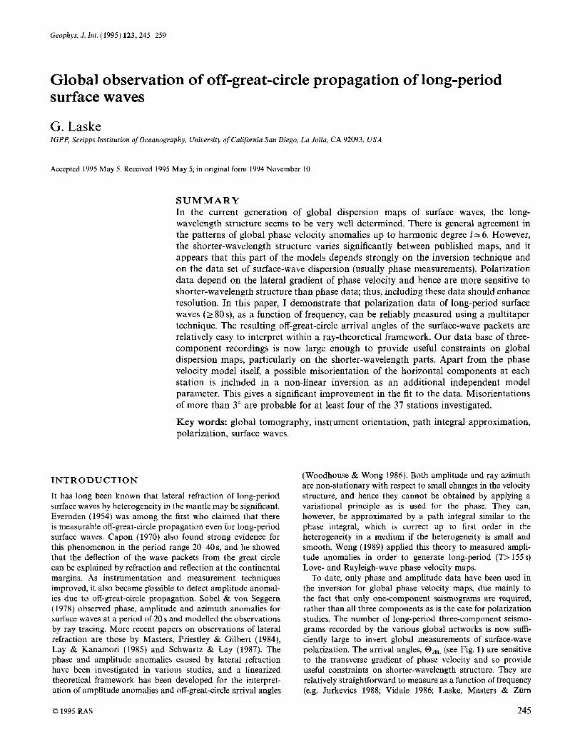
Geophys. J . Int. (1995) 123,245-259

Global observation of off-great-circle propagation of long-period surface waves

G. Laske IGPP, Scripps Institution of Oceanography, University of Calijornia San Diego, La Jolla, CA 92093, USA

Accepted 1995 May 5. Received 1995 May 5; in original form 1994 November 10

SUMMARY In the current generation of global dispersion maps of surface waves, the long- wavelength structure seems to be very well determined. There is general agreement in the patterns of global phase velocity anomalies up to harmonic degree 1-6. However, the shorter-wavelength structure varies significantly between published maps, and it appears that this part of the models depends strongly on the inversion technique and on the data set of surface-wave dispersion (usually phase measurements). Polarization data depend on the lateral gradient of phase velocity and hence are more sensitive to shorter-wavelength structure than phase data; thus, including these data should enhance resolution. In this paper, I demonstrate that polarization data of long-period surface waves (2 80 s), as a function of frequency, can be reliably measured using a multitaper technique. The resulting off-great-circle arrival angles of the surface-wave packets are relatively easy to interpret within a ray-theoretical framework. Our data base of three- component recordings is now large enough to provide useful constraints on global dispersion maps, particularly on the shorter-wavelength parts. Apart from the phase velocity model itself, a possible misorientation of the horizontal components at each station is included in a non-linear inversion as an additional independent model parameter. This gives a significant improvement in the fit to the data. Misorientations of more than 3" are probable for at least four of the 37 stations investigated.

Key words: global tomography, instrument orientation, path integral approximation, polarization, surface waves.

INTRODUCTION

It has long been known that lateral refraction of long-period surface waves by heterogeneity in the mantle may be significant. Evernden (1954) was among the first who claimed that there is measurable off-great-circle propagation even for long-period surface waves. Capon (1970) also found strong evidence for this phenomenon in the period range 20-4Os, and he showed that the deflection of the wave packets from the great circle can be explained by refraction and reflection at the continental margins. As instrumentation and measurement techniques improved, it also became p"ossib1e to detect amplitude anomal- ies due to off-great-circle propagation. Sobel & von Seggern (1978) observed phase, amplitude and azimuth anomalies for surface waves at a period of 20s and modelled the observations by ray tracing. More recent papers on observations of lateral refraction are those by Masters, Priestley & Gilbert (1984), Lay & Kanamori (1985) and Schwartz & Lay (1987). The phase and amplitude anomalies caused by lateral refraction have been investigated in various studies, and a linearized theoretical framework has been developed for the interpret- ation of amplitude anomalies and off-great-circle arrival angles

(Woodhouse & Wong 1986). Both amplitude and ray azimuth are non-stationary with respect to small changes in the velocity structure, and hence they cannot be obtained by applying a variational principle as is used for the phase. They can, however, be approximated by a path integral similar to the phase integral, which is correct up to first order in the heterogeneity in a medium if the heterogeneity is small and smooth. Wong (1989) applied this theory to measured ampli- tude anomalies in order to generate long-period (I, 155 s) Love- and Rayleigh-wave phase velocity maps.

To date, only phase and amplitude data have been used in the inversion for global phase velocity maps, due mainly to the fact that only one-component seismograms are required, rather than all three components as is the case for polarization studies. The number of long-period three-component seismo- grams recorded by the various global networks is now suffi- ciently large to invert global measurements of surface-wave polarization. The arrival angles, OZH, (see Fig. 1) are sensitive to the transverse gradient of phase velocity and so provide useful constraints on shorter-wavelength structure. They are relatively straightforward to measure as a function of frequency (e.g. Jurkevics 1988; Vidale 1986; Laske, Masters & Ziirn

0 1995 RAS 245

246 G. Laske

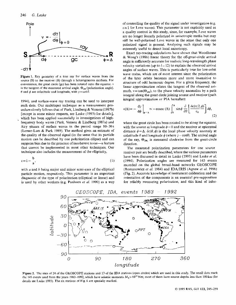
Pole t

" =-- . dY I I

@ = A

-dY 'I Cl@

Figure 1. Ray geometry of a true ray for surface waves from the source (S) to the receiver (R) through a heterogeneous medium. For convenience, the great circle (gc) has been rotated onto the equator. v is the tangent of the measured arrival angle, OZH (polarization angle). 0 and 4 are colatitude and longitude, with y = cot 0.

1994), and surface-wave ray tracing can be used to interpret such data. Our multitaper technique as a measurement pro- cedure closely follows that of Park, Lindberg & Vernon (1987b) [except in some minor respects, see Laske (1993) for details], which has been applied successfully in investigations of high- frequency body waves (Park, Vernon & Lindberg 1987a) and Airy phases of surface waves in the period range 10-30s (Lerner-Lam & Park 1989). The method gives an estimate of the quality of the observed signal (in the sense that its particle motion can be described by one polarization ellipse) and can suppress bias due to the presence of incoherent noise-a feature that cannot be implemented in most other techniques. Our technique also includes the measurement of the ellipticity,

with a and b being major and minor semi-axes of the elliptical particle motion, respectively. This parameter is an important diagnostic of the type of polarization (elliptical or linear) and is used by other workers (e.g. Paulssen et al. 1990) as a way

of controlling the quality of the signal under investigation (e.g. E N 1 for Love waves). This parameter is not explicitly used as a quality control in this study, since, for example, Love waves are no longer linearly polarized in anisotropic media but may still be well-polarized Love waves in the sense that only one polarized signal is present. Analysing such signals may be extremely useful to detect local anisotropy.

Exact ray-tracing calculations have shown that Woodhouse & Wong's (1986) linear theory for the off-great-circle arrival angle is sufficiently accurate for realistic long-wavelength phase velocity variations (up to I = 12) to explain the observed arrival angles of surface waves. This is particularly true for low-orbit wave trains, which are of most interest since the polarization of the later orbits becomes more and more insensitive to structure of odd harmonic degree. For a given frequency, the linear approximation relates the tangent of the observed azi- muth, v = tan(@),,), to the phase velocity anomalies by a path integral along the great circle joining source and receiver (path integral approximation or PIA hereafter):

( 2 )

where the great circle has been rotated to be along the equator, with the source at longitude 4 = 0 and the receiver at epicentral distance 4 = A . 6c(B, 4) is the local phase velocity anomaly at colatitude 0 and longitude 4 (where y=cotQ). The arrival angle of the ray, @2H, is measured clockwise from the great-circle direction.

The measured polarization parameters for one source- receiver pair are briefly described, where the various parameters have been discussed in detail in Laske (1993) and Laske et al. (1994). Polarization angles are measured for 145 events recorded on the global broad-band networks GEOSCOPE (Romanowicz et at. 1984) and IDA/IRIS (Agnew et af. 1986) (Fig. 2). Accurate knowledge of instrument calibration and the orientation of the components is an essential pre-supposition for reliably measuring polarization, and this kind of infor-

GEOSCOPE, IDA, even t s 1983 - 1992 90

60

30

0

-30

-60

-.90 _ _ 0 90 180 2 70 360

long i tude Figure 2. The sites of 24 of the GEOSCOPE stations and 13 of the IDA stations (open circles) which are used in this study. The small dots mark the 145 events used from the years 1983-1992, which have seismic moments Mo> 10"Nm; most of them have source depths less than lOOkm (for details see Laske 1993). The six stations of Fig. 6 are specially marked.

0 1995 RAS, GJI 123, 245-259

Off-great-circle propagation 247

Year

1983 - 1987 1988 1989 1990 1991 1992

c

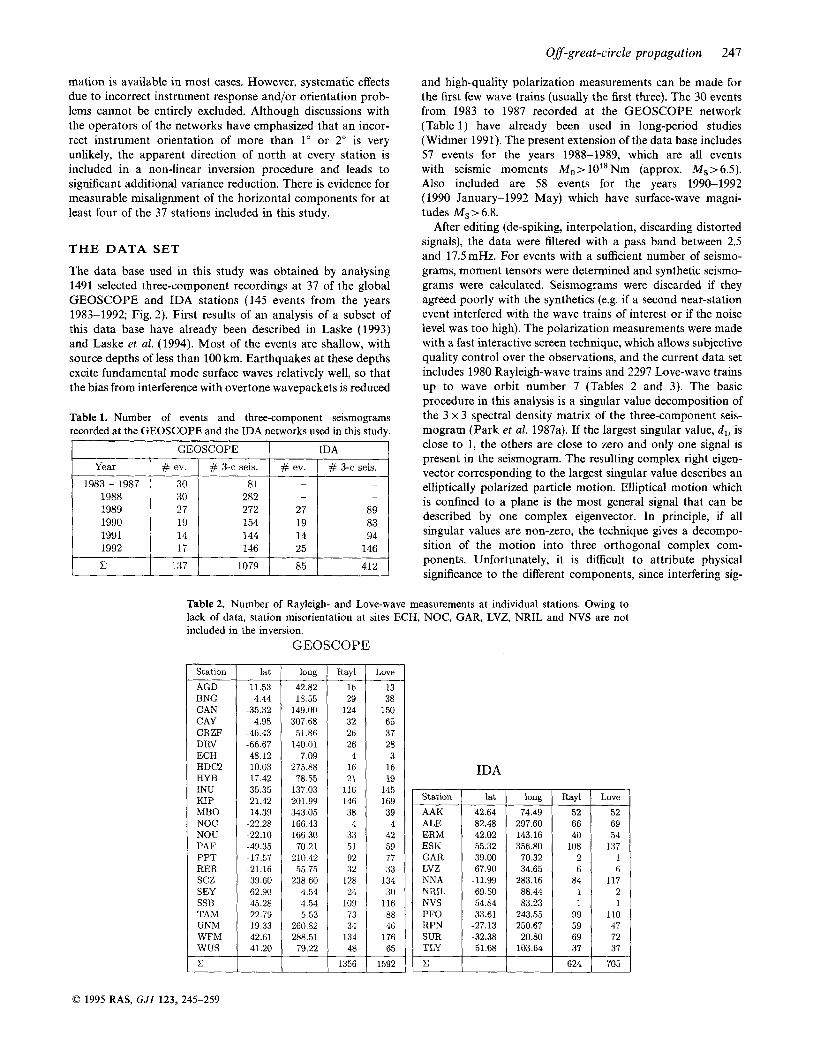
mation is available in most cases. However, systematic effects due to incorrect instrument response and/or orientation prob- lems cannot be entirely excluded. Although discussions with the operators of the networks have emphasized that an incor- rect instrument orientation of more than 1" or 2" is very unlikely, the apparent direction of north at every station is included in a non-linear inversion procedure and leads to significant additional variance reduction. There is evidence for measurable misalignment of the horizontal components for at least four of the 37 stations included in this study.

GEOSCOPE IDA # ev. # 3-c seis. # ev. # 3-c seis.

30 81 - -

30 282 - -

27 272 27 89 19 154 19 83 14 144 14 94 17 146 25 146

137 1079 85 412

THE DATA SET

The data base used in this study was obtained by analysing 1491 selected three-component recordings at 37 of the global GEOSCOPE and IDA stations (145 events from the years 1983-1992; Fig. 2). First results of an analysis of a subset of this data base have already been described in Laske (1993) and Laske et al. (1994). Most of the events are shallow, with source depths of less than 100 km. Earthquakes at these depths excite fundamental mode surface waves relatively well, so that the bias from interference with overtone wavepackets is reduced

and high-quality polarization measurements can be made for the first few wave trains (usually the first three). The 30 events from 1983 to 1987 recorded at the GEOSCOPE network (Table 1) have already been used in long-period studies (Widmer 1991). The present extension of the data base includes 57 events for the years 1988-1989, which are all events with seismic moments M , > 10" Nm (approx. M s > 6.5). Also included are 58 events for the years 1990-1992 ( 1990 January-1992 May) which have surface-wave magni- tudes Ms > 6.8.

After editing (de-spiking, interpolation, discarding distorted signals), the data were filtered with a pass band between 2.5 and 17.5mHz. For events with a sufficient number of seismo- grams, moment tensors were determined and synthetic seismo- grams were calculated. Seismograms were discarded if they agreed poorly with the synthetics (e.g. if a second near-station event interfered with the wave trains of interest or if the noise level was too high). The polarization measurements were made with a fast interactive screen technique, which allows subjective quality control over the observations, and the current data set includes 1980 Rayleigh-wave trains and 2297 Love-wave trains up to wave orbit number 7 (Tables 2 and 3). The basic procedure in this analysis is a singular value decomposition of the 3 x 3 spectral density matrix of the three-component seis- mogram (Park et al. 1987a). If the largest singular value, d,, is close to 1, the others are close to zero and only one signal is present in the seismogram. The resulting complex right eigen- vector corresponding to the largest singular value describes an elliptically polarized particle motion. Elliptical motion which is confined to a plane is the most general signal that can be described by one complex eigenvector. In principle, if all singular values are non-zero, the technique gives a decompo- sition of the motion into three orthogonal complex com- ponents. Unfortunately, it is difficult to attribute physical significance to the different components, since interfering sig-

Table 2. Number of Rayleigh- and Love-wave measurements at individual stations. Owing to lack of data, station misorientation at sites ECH, NOC, GAR, LVZ, NRIL and NVS are not included in the inversion.

GEOSCOPE

Station

AGD BNG CAN CAY CRZF DRV ECH HDC2 HYB INU KIP MBO NOC NOU PAF PPT RER scz SEY SSB TAM UNM WFM WUS c

lat

11.53 4.44

-35.32 4.95

-46.43 -66.67 48.12 10.03 17.42 35.35 21.42 14.39

-22.28 -22.10 -49.35 -17.57 -21.16 39.60 C2.90 45.28 22.79 19.33 42.61 41.20

long

42.82 18.55

149.00 307.68 51.86

140.01 7.09

275.88 78.55

137.03 201.99 343.05 166.43 166 30 70.21

210.42 55 75

238.60 4.54 4.54 5.53

260.82 288.51 79.22

R ayl

16 29

124 32 26 26

4 16 21

116 146 38 4

33 51 92 32

128 24

109 73 34

134 48

1356

__

__

Love

13 38

150 65 37 28 3

16 19

145 169 39 4

42 59 77 33

134 30

116 88 46

176 65

1592 __

IDA

Station

42.64 82.48

55.32

67.90

54.84 PFO 33.61

TLY 51.68

long

74.49 297.60 143.16 356.80

70.32 34.65

283.16 88.44 83.23

243.55 250.67 20.80

103.64

Ray1 52 66 40

108 2 6

84 1 1

99 59 69 37

624

-

-

Love

52 69 54

137 1 6

117 2 1

110 47 72 37

705 -

0 1995 RAS, GJI 123,245-259

248 G. Laske

wave orbit # 1

Rayleigh 845

Love 842

2 3 4 5 6 7

678 309 97 42 9 0

774 449 185 39 7 1

nals are generally not orthogonally polarized. Moreover, spec- tral leakage, especially in the presence of noise, can mimic the existence of more than one signal (Laske 1993). Hence, it is not feasible to extract the desired signal from a conglomerate of incoming waves, but the magnitude of the largest singular value, dl, provides a good way of estimating the quality of the observed signal. In this study, measurements with d , ~ 0 . 8 0 were discarded.

The lack of high-precision polarization measurements for higher orbits is caused by the increasingly poor signal-to-noise ratio as the wave orbit number increases. The relatively strong dispersion of Rayleigh waves also forces the data windows to be larger for wave trains with higher orbit numbers, which increases the probability that more interfering signals are present. This is one of the reasons that there are more Love- than Rayleigh-wave observations in our data set for wave orbit numbers 2-4. It is also fairly common to find that, in the same seismogram, it is possible to obtain high-precision Love-wave measurements but no Rayleigh-wave measurements, because the different types of wave packet overlap. For example, at epicentral distances 30" 5 A I 50", GI overlaps with R1, and G3 with R2 at frequencies 10-20 mHz; hence, measurements can be obtained for G2 but not for the other wave trains. Since the wave trains overlap over a large frequency band, the

moving window technique as described in Laske et al. (1994) gives no further improvement in this particular case.

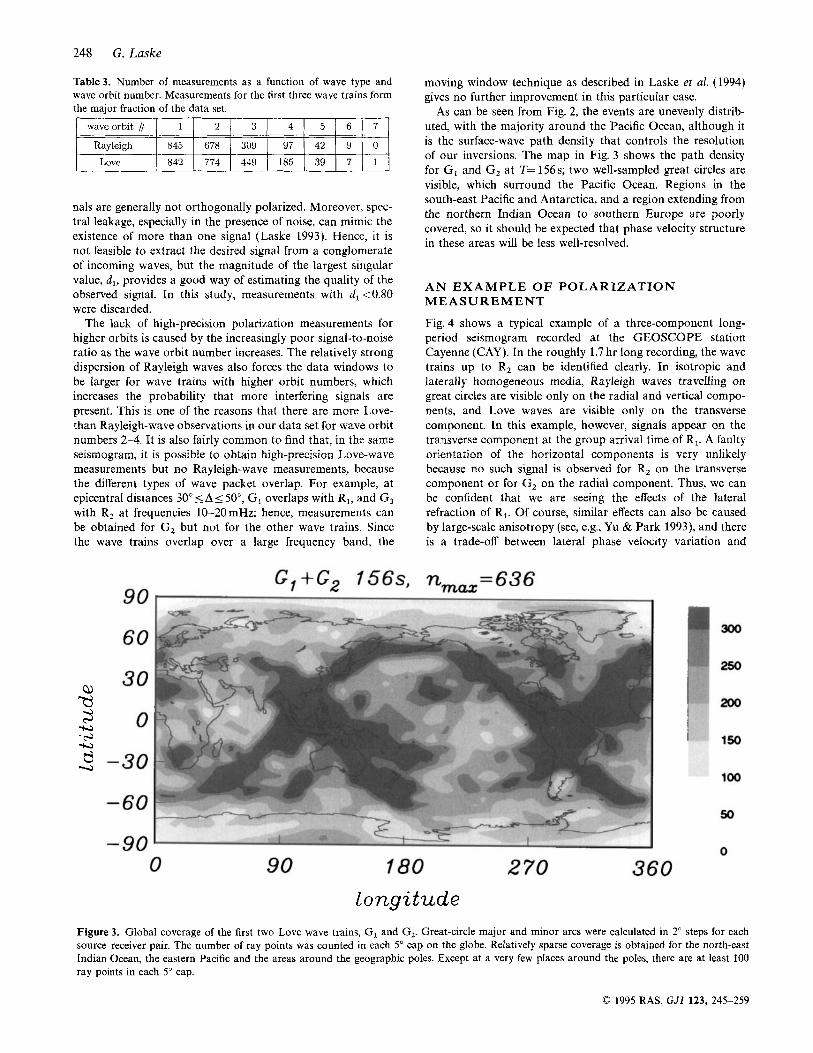
As can be seen from Fig. 2, the events are unevenly distrib- uted, with the majority around the Pacific Ocean, although it is the surface-wave path density that controls the resolution of our inversions. The map in Fig. 3 shows the path density for GI and G2 at T= 156s; two well-sampled great circles are visible, which surround the Pacific Ocean. Regions in the south-east Pacific and Antarctica, and a region extending from the northern Indian Ocean to southern Europe are poorly covered, so it should be expected that phase velocity structure in these areas will be less well-resolved.

l ong i tude

AN EXAMPLE O F POLARIZATION MEASUREMENT

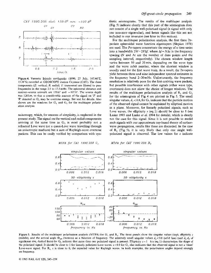
Fig. 4 shows a typical example of a three-component long- period seismogram recorded at the GEOSCOPE station Cayenne (CAY). In the roughly 1.7 hr long recording, the wave trains up to R, can be identified clearly. In isotropic and laterally homogeneous media, Rayleigh waves travelling on great circles are visible only on the radial and vertical compo- nents, and Love waves are visible only on the transverse component. In this example, however, signals appear on the transverse component at the group arrival time of R,. A faulty orientation of the horizontal components is very unlikely because no such signal is observed for R, on the transverse component or for G2 on the radial component. Thus, we can be confident that we are seeing the effects of the lateral refraction of R,. Of course, similar effects can also be caused by large-scale anisotropy (see, e.g., Yu & Park 1993), and there is a trade-off between lateral phase velocity variation and

Figure 3. Global coverage of the first two Love wave trains, GI and G2. Great-circle major and minor arcs were calculated in 2" steps for each source-receiver pair. The number of ray points was counted in each 5" cap on the globe. Relatively sparse coverage is obtained for the north-east Indian Ocean, the eastern Pacific and the areas around the geographic poles. Except at a very few places around the poles, there are at least 100 ray points in each 5" cap.

0 1995 RAS, GJI 123, 245-259

08-great-circle propagation 249

CAY 1990 208 dzst 139 6 O a m -107 8 O

K1 G2 R2

0 8 1 2 7 6 2 0 1 Lme/h

Figure 4. Vanuatu Islands earthquake (1990, 27 July, 167.46"E, 15.365) recorded at GEOSCOPE station Cayenne (CAY). The three components ( 2 vertical; R: radial; li transverse) are filtered to pass frequencies in the range 2.5 to 17.5 mHz. The epicentral distance and receiver-source azimuth are 139.6" and - 107.8". The source depth was 126 km, so that a considerable amount of the signal on 'Z' and 'R' denoted as G, may be overtone energy. See text for details. Also shown are the windows for G1 and G, for the multitaper polariz- ation analysis.

anisotropy, which, for reasons of simplicity, is neglected in the present study. The signal on the vertical and radial components arriving at the same time as GI is most probably not a refracted Love wave (or a quasi-Love wave travelling through an anisotropic medium) but a sum of Rayleigh-wave overtone packets. This can be easily verified by comparison with syn-

MTPA f o r CAY 1990.208 G ,

s ingu lar va Lues

/ 0.4

0.0 ' , I -

.--.__ /-;-Tpy .,-- 1- - - f ._ , -

0.006 0.012 0.018

30 -e l l ip t ic i ty E

O " L 0.4 0.0

0.006 0.012 0.018

02,

, 2 0 7 1 100

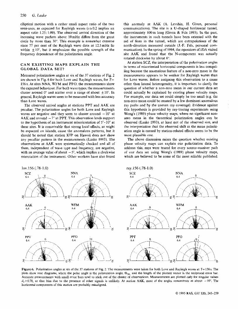
thetic seismograms. The results of the multitaper analysis (Fig. 5) indicate clearly that this part of the seismogram does not consist of a single well-polarized signal (a signal with only one non-zero eigenvalue), and hence signals like this are not included in our inversion (see later in this section).

For the multitaper polarization analysis, the first three 27r- prolate spheroidal wave function eigentapers (Slepian 1978) are used. The Px-tapers concentrate the energy of a time series into a bandwidth 2W=2PAJ where Af=NAt is the frequency spacing (N and At are the number of data points and the sampling interval, respectively). The chosen window length varies between 10 and 35min, depending on the wave type and the wave orbit number, where the shortest window is usually used for the first wave train. As a result, the 2n-tapers yield between three and nine independent spectral estimates in the frequency band 2-20 mHz. Unfortunately, the frequency resolution is relatively poor for the first-arriving wave packets, but possible interference with other signals (other wave type, overtones) does not allow the choice of longer windows. The results of the multitaper polarization analysis of R, and GI for the seismogram of Fig. 4 are plotted in Fig. 5. The small singular values, dl < O X , for G1 indicate that the particle motion of the observed signal cannot be explained by elliptical motion in a plane. Moreover, for linearly polarized signals, such as Love waves, the ellipticity E (eq.1) should be close to 1 (see Laske 1993 and Laske et al. 1994 for details), which is clearly not the case for this signal. Since it is not possible to model such signals with our approximate ray-based theory of surface- wave propagation, results like these are discarded. In the case of R, (Fig. 5 ) , it is very likely that only one single well- polarized signal is observed. The low values for E indicate

MTPA f o r CAY 1990.208 R,

s ingu lar v a l u e s

0.0 0.006 0.012 0.018

3D-ellipticity E

0.006 0.012 0.018

02"

0.006 0012 0.018 0.006 0.012 0.018 f r e q u e n c y in H z f r e q u e n c y in H z

Figure 5. Results of the multitaper polarization analysis (MTPA) for G, and R,. The three panels show the singular values (top), ellipticity E

(middle), and the arrival angle 0," (bottom) as a function of frequency. The relatively small singular values d,<0.8 (solid line) (and d,.d, of significant size, dashed lines) for G, indicate that more than one polarized signal is present. Ellipticity E = 1 - b/a (eq. 1) characterizes the shape of the polarized signal. It should be close to 1 for linearly polarized Love waves. ~ i 0 . 9 for G, also indicates that the observed signal is not a 'clean' Love-wave signal. For R,, E is close to 0, the expected value for Rayleigh waves. In both examples, the polarization angles depend strongly on frequency.

0 1995 RAS, GJI 123, 245-259

250 G. Laske

elliptical motion with a rather small aspect ratio of the two semi-axes, as expected for Rayleigh waves ( ~ ~ 0 . 2 implies an aspect ratio 1.25 : 1.00). The observed arrival direction of the incoming wave packets above 10mHz differs from the great circle by more than 30". This example is somewhat extreme since 77 per cent of the Rayleigh wave data at 12.5mHz lie within +lo", but it emphasizes the possible strength of the frequency dependence of the polarization angle.

C A N EXISTING MAPS EXPLAIN THE GLOBAL DATA SET?

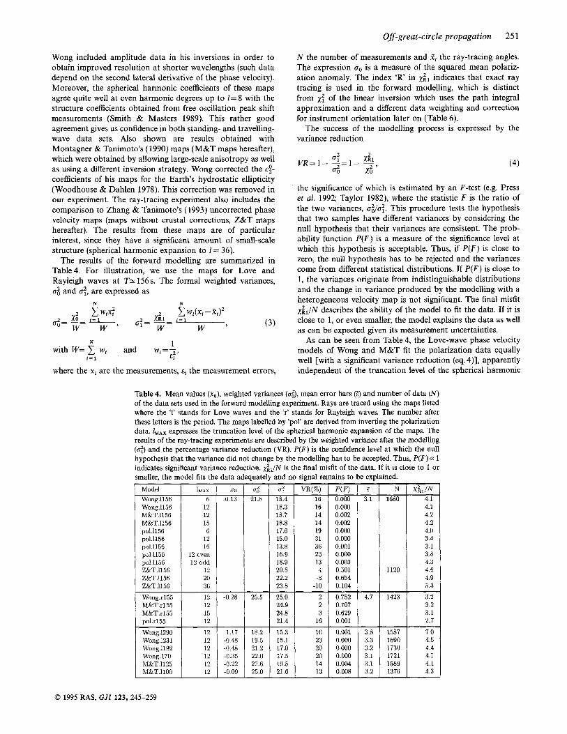
Measured polarization angles at six of the 37 stations of Fig. 2 are shown in Fig. 6 for both Love and Rayleigh waves, for T= 156 s. At sites NNA, WFM and PFO, the measurements show the expected behaviour. For both wave types, the measurements cluster around 0" and scatter over a range of about f 10". In general, Rayleigh waves seem to be measured with less accuracy than Love waves.

The observed arrival angles at stations PPT and AAK are peculiar. The polarization angles for both Love and Rayleigh waves are negative and they seem to cluster around -10" at AAK and around - 7" at PPT. This observation lends support to the hypothesis of an instrument misorientation of So-10" at these sites. It is conceivable that strong local effects, as might be expected on islands, cause the anomalous patterns, but it should be noted that station KIP on Hawaii does not show any peculiar pattern in the measurements (Laske 1993). The observations at AAK were systematically checked and all of them, independent of wave type and frequency, are negative, with an average value of about - 5", which implies a clockwise misrotation of the instrument. Other workers have also found

lov.156 (.78-1.0) scz NNA

0 6.4 AAK 6.4

this anomaly at AAK (A. Levshin, H. Given, personal communications). The site is a U-shaped horizontal tunnel, approximately 100m long (Given & Fels 1993). In the past, the instruments in such tunnels have been oriented with the aid of lines in the tunnel, which are extrapolations of the north-direction measured outside (J.-F. Fels, personal com- munication). In the spring of 1994, the operators of IDA visited site AAK and found that the N-component was actually rotated clockwise by about 6".

At station SCZ, the interpretation of the polarization angles in terms of misoriented horizontal components is less compel- ling because the anomalous feature of a non-zero mean in the measurements appears to be weaker for Rayleigh waves than for Love waves. Before assigning this observation to a cause other than lateral heterogeneity, it is important to clarify the question of whether a non-zero mean in our current data set could actually be explained by existing phase velocity maps. For example, our data set could simply be too small (e.g. the non-zero mean could be created by a few dominant anomalous ray paths and by the uneven ray coverage). Evidence against this hypothesis is provided by ray-tracing experiments using Wong's (1989) phase velocity maps, where no significant non- zero mean in the theoretical polarization angles can be observed (Laske 1993), at least not of the observed size, and the interpretation that the observed shift in the mean polariz- ation angle is caused by station-related effects seems to be the most plausible one.

The above discussion raises the question whether existing phase velocity maps can explain our polarization data. To address this, rays were traced for every source-receiver path of our data set using Wong's (1989) phase velocity maps, which are believed to be some of the most reliable published.

ray.156 (.78-1.0) scz NNA

AAK WFM

w 0 0 w o m Or?

PPT PFO I

Figure 6. Polarization angles at six of the 37 stations of Fig. 2. The measurements were taken for both Love and Rayleigh waves at T= 156s. The plots show rose diagrams, where the polar angle is the polarization angle, G2", and the length of the plotted vector is the reciprocal error bar. Accurate measurements with small error bars tend to stick out of the cluster of observations. Measurements are plotted only for singular values d , 20.78, so that bias due to the presence of other signals is unlikely. At station AAK, most of the angles concentrate at about - 10". The horizontal components of this station are probably misaligned.

0 1995 RAS, GJI 123, 245-259

08-great-circle propagation 251

P ( F ) 0.000 0.000 0.002 0.002 0.000 0.000 0.001 0.000 0.003 0.501 0.654 0.104

0.752 0.707 0.629 0.001

Wong included amplitude data in his inversions in order to obtain improved resolution at shorter wavelengths (such data depend on the second lateral derivative of the phase velocity). Moreover, the spherical harmonic coefficients of these maps agree quite well at even harmonic degrees up to 1=8 with the structure coefficients obtained from free oscillation peak shift measurements (Smith & Masters 1989). This rather good agreement gives us confidence in both standing- and travelling- wave data sets. Also shown are results obtained with Montagner & Tanimoto’s (1990) maps (M&T maps hereafter), which were obtained by allowing large-scale anisotropy as well as using a different inversion strategy. Wong corrected the c;- coefficients of his maps for the Earth’s hydrostatic ellipticity (Woodhouse & Dahlen 1978). This correction was removed in our experiment. The ray-tracing experiment also includes the comparison to Zhang & Tanimoto’s ( 1993) uncorrected phase velocity maps (maps without crustal corrections, Z&T maps hereafter). The results from these maps are of particular interest, since they have a significant amount of small-scale structure (spherical harmonic expansion to 1 = 36).

The results of the forward modelling are summarized in Table4. For illustration, we use the maps for Love and Rayleigh waves at TE 156 s. The formal weighted variances, 0; and c!, are expressed as

N N

t N 3.1 1680

1129

4.7 1423

N 1 with W= wi and wi=-

i = l E: ’

Model Wong.1156 Wong.1156 M8~T.1156 M&T.1156 po1.1156 po1.1156 po1.1156 po1.1156 po1.1156 Z8~T.1156 Z&T.1156 Z8zT.1156

Wong.rl55 M&T.r155 M&T.r155 pol.rl55

Wong.1290 Wong.1231 Wong.1192 Wong.170 M&T.1125 M&T.1100

where the xi are the measurements, E~ the measurement errors,

A MAX 6

12 12 15 6

12 16

12 even 12 odd

12 20 36

12 12 15 12

12 12 12 12 12 12

N the number of measurements and Ti the ray-tracing angles. The expression no is a measure of the squared mean polariz- ation anomaly. The index ‘ R in xil indicates that exact ray tracing is used in the forward modelling, which is distinct from x: of the linear inversion which uses the path integral approximation and a different data weighting and correction for instrument orientation later on (Table 6).

The success of the modelling process is expressed by the variance reduction

(4)

the significance of which is estimated by an F-test (e.g. Press et al. 1992; Taylor 1982), where the statistic F is the ratio of the two variances, u;/u:. This procedure tests the hypothesis that two samples have different variances by considering the null hypothesis that their variances are consistent. The prob- ability function P ( F ) is a measure of the significance level at which this hypothesis is acceptable. Thus, if P ( F ) is close to zero, the null hypothesis has to be rejected and the variances come from different statistical distributions. If P ( F ) is close to 1, the variances originate from indistinguishable distributions and the change in variance produced by the modelling with a heterogeneous velocity map is not significant. The final misfit xil/N describes the ability of the model to fit the data. If it is close to 1, or even smaller, the model explains the data as well as can be expected given its measurement uncertainties.

As can be seen from Table 4, the Love-wave phase velocity models of Wong and M&T fit the polarization data equally well [with a significant variance reduction (eq. 4)], apparently independent of the truncation level of the spherical harmonic

Table 4. Mean values (X,,), weighted variances (of), mean error bars (E) and number of data ( N ) of the data sets used in the forward modelling experiment. Rays are traced using the maps listed where the ‘1’ stands for Love waves and the ‘r’ stands for Rayleigh waves. The number after these letters is the period. The maps labelled by ‘pol’ are derived from inverting the polarization data. I,,, expresses the truncation level of the spherical harmonic expansion of the maps. The results of the ray-tracing experiments are described by the weighted variance after the modelling (a:) and the percentage variance reduction (VR). P ( F ) is the confidence level at which the null hypothesis that the variance did not chalj indicates significant variance reduction. 2 smaller, the model fits the data adeauate

-0.35

-0.09

by the modelling has to be accepted. Thus, P ( F ) e 1 ‘N is the final misfit of the data. If it is close to 1 or and no signal remains to be explained. - d -

18.4 18.3 18.7 18.8 17.6 15.0 13.8 16.9 18.9 20.8 22.2 23.8

25.0 24.9 24.8 21.4

-

15.3 15.1 17.0 17.5 19.5 21.6 -

I - VR(%)

16 16 14 14 19 31 36 23 13 4

-3 -10

2 2 3

16

16 23 20 20 14 13

I

0.000 1730 0.000 1721

&,IN 4.1 4.1 4.2 4.2 4.0 3.4 3.1 3.8 4.3 4.6 4.9 5.3

3.2 3.2 3.1 2.7

7.0 4.5 4.4 4.1 4.1 4.3

0 1995 RAS, GJI 123, 245-259

252 G. Laske

expansion. It is interesting to note that the Z&T maps cannot explain our data, particularly if the short-wavelength structure is included in the ray-tracing model. Since the phase velocity maps of different authors roughly agree up to 1=6 (Laske 1993), one might conclude from this either that shorter- wavelength structure is not required to explain the polarization data or that the measurements are not accurate enough to constrain global phase velocity maps. It is commonly assumed that the spectrum of the Earth's 3-D structure is very 'red' (Su & Dziewonski 1991) and that the amplitude in the phase velocity maps drops approximately as l/l, and so contributions in the model above 1=6 are expected to be small. Recall, however, that the polarization data are sensitive to shorter- wavelength structure, particularly if it leads to strong lateral phase velocity gradients. The variance reduction of roughly 15 per cent for the existing models, which are derived using only phase data, is rather small [although it is highly significant, P(F)<O.Ol], and it is expected that an inversion including polarization data will lead to models that fit the latter much better (and still fit the phase data). A glance at the variance reduction, using maps that were obtained from a preliminary inversion using only polarization measurements (see next sec- tion), shows that structure at 1>6 is actually required to improve the fit of the polarization data.

The ray-tracing experiment was also carried out for Rayleigh waves, and it is interesting to note that existing phase velocity maps cannot explain our polarization data set (no significant variance reduction). The initial variance at T= 155 s is slightly higher than for Love waves at the same period (compare 25.5 with 21.8). This is somewhat surprising because the amplitude of the phase velocity anomaly is smaller for Rayleigh waves than for Love waves at the same period, and so smaller polarization angles and thus a smaller variance in the data are expected. However, since the average measurement error is 1.5 times larger, the final misfit is smaller and less significant signal remains to be explained after the forward modelling.

Also shown in Table 4 are results for Love waves obtained at a variety of periods. Since Wong's models are available only for periods longer than 15Os, the modelling at shorter periods was performed with the M&T maps. The initial variance of the polarization data, ci, increases with frequency. This behav- iour is expected, as the phase velocity models become rougher at shorter periods, with higher peak-to-peak phase velocity anomalies, varying from -3.2 to 3.1 per cent for T=29Os up to - 5.0 to 4.5 per cent for T= 156 s. The greater final misfit at longer periods is somewhat surprising, since it might be expected that long-period surface waves should be only weakly deflected from the great circle. Several explanations are poss- ible: (1) larger mean errors indicate that the measurements for these periods are less accurate; (2) the measurements may be biased by the effects of spectral leakage, which is more severe at longer periods (since Aflfis larger); ( 3 ) greater dispersion at longer periods makes it difficult to choose a window that includes all of the desired signal; (4) mode coupling due to the Earth's rotation becomes stronger and ( 5 ) ray-based theories start to fail at long periods (if short-wavelength structure is present) (see also Park 1989).

THE FORMULATION OF THE INVERSION

Ideally, if the data coverage were perfect, the resulting model of an inversion would not depend on its parameterization. In

seismic tomography, basically two types of parameterization have become established. The first one is a block parameteriz- ation, in which the area to be investigated is divided into cells of a certain geometry (triangles, squares, etc.). Such a para- meterization is commonly applied in regional studies, but examples can also be found in global surface-wave tomography (e.g. Zhang & Tanimoto 1993). The other technique involves the expansion of the model into global basis functions, for example surface spherical harmonics in the case of global surface-wave tomography (Wong 1989). Each of these tech- niques has its advantages, but also its drawbacks. The block parameterization allows an inversion for structure on a very small scale where data are available. However, it tends to produce artefacts in regions with poor data coverage. An expansion of a global model into spherical harmonics up to relatively low harmonic degree does not allow sharp edges in the model (e.g. continent-ocean boundaries), and the inverted model will probably be a low-pass-filtered version of the true model. On the other hand, the small-scale artefacts due to poor data coverage are easier to suppress with this parameteriz- ation by applying appropriate smoothing constraints. Since we may assume that the Earth's 3-D structure is dominated by long wavelengths (Su & Dziewonski 1991), the latter parameterization appears to be the more appropriate one for our inversion.

The global phase velocity anomaly with respect to its spherical average, co, is expanded in spherical surface harmon- ics as

( 5 )

where y;" are the fully normalized surface spherical harmonics (Edmonds 1960). Our polarization data depend on the lateral gradient of phase velocity anomaly and, using eq. (2), are thus also linear functions of the spherical harmonic coefficients, Cr":

- J Y d m A

where d is the data vector, m is the model vector and A is the data kernel matrix. In the presence of noise, the linear forward problem is expressed as

d = Am+e, ( 7 )

where e is the error vector. Since the arrival angle is sensitive only to the lateral velocity gradient and not to the velocity itself, the coefficient c: cannot be obtained by the inversion of polarization data alone.

There are many more data than parameters to invert, so the problem in question is formally overdetermined; however, due to our limited number of data and the uneven global coverage, the inverse problem is underconstrained. To circumvent the difficulties of inverting an ill-conditioned matrix, various forms of iegularization (or damping) can be introduced (e.g. using the method of Lagrange multipliers), which constrain the model to meet some specific requirements. One possibility is the search for smooth models. The task is then to find the minimum of the weighted sum of the data error vector (or

0 1995 RAS, GJI 123, 245-259

Off-great-circle propagation 253

prediction error) and the roughness of the model,

eTe + qZmTaTam, (8)

where a is a roughness operator.

Laplacian, V:, where The roughness of a model, dm, is expressed by the surface

(9)

and SZ is the surface of the sphere (Woodward & Masters 1992). Since there is a trade-off between the misfit of the data and the roughness of the model, the regularization parameter q should be chosen so that the model has the desired smooth- ness but is still able to fit the data within a tolerable limit. The inverse problem is then expressed by m = Gd where the inverse matrix G is given by

G = [ATA + $aTa] AT. ( 10)

If the phase velocity perturbation is expanded in spherical harmonics, we have

lam12=x 1 1 2 ( 1 + 1)21c;”12,

so that the inverse matrix G becomes I m

G = [ATA + q212 (1+ l)21]-1AT.

Another type of constraint that is commonly used results in the search for a model with the shortest possible model vector length giving G = [ATA + q21] -lAT. This constraint has the drawback that it can map large-scale heterogeneity into

orbit I 20 15

shorter-wavelength structure (Laske 1993). If we believe that phase velocity maps are dominated by large-scale structure, this constraint is not optimal and is not used in the inversion presented here.

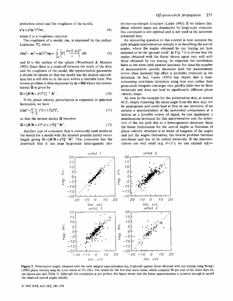
An interesting question in this context is how accurate the path integral approximation actually is in describing the arrival angles, where the angles obtained by ray tracing are here assumed to be the ‘ground truth’. In Fig. 7 it is shown that the angles obtained with the linear theory agree very well with those obtained by ray tracing. As expected, the correlation fades as the wave orbit number increases, but since the number of measurements quickly decreases (and the measurement errors often increase) this effect is probably irrelevant in the inversion. In fact, Laske (1993) has shown that a time- consuming non-linear inversion using true rays rather than great-circle integrals converges very quickly (after two or three iterations) and does not lead to significantly different phase velocity maps.

As seen in the example for the polarization data at station SCZ, simply removing the mean angle from the data may not be appropriate and could lead to bias in our inversion. If we assume a misorientation of the horizontal components at a station as a possible source of signal, we can implement a simultaneous inversion for this misorientation and the deflec- tion of the ray path due to a heterogeneous structure. Since the linear formulation for the arrival angles as functions of phase velocity structure is in terms of tangents of the angles and not the angles themselves, the inverse problem becomes non-linear and has to be solved iteratively. If the misorien- tations are very small (e.g. 8 < 5 ” ) , we can expand v(A)=

orb i t 2 20 15 I

-20 -10 0 10 20 -20 -10 0 10 20 Lin. es t . o r b i t 3

20 15

l in . est. orbi t 4

-201’ 1 1 1 i ’ ’ -20 - 1 0 0 10 20 -20 -10 0 10 20

Lin. es t . Lin. es t

Figure 7. Polarization angles obtained with the path integral approximation (eq. 2) plotted against those obtained with ray tracing using Wong’s (1989) phase velocity map for Love waves at T= 156 s. The results for the first four wave trains, which comprise 98 per cent of the entire data set, are shown (see also Table 3). Although the correlation is not perfect, this figure shows that the linear approximation is accurate enough to model the observed arrival angles reliably.

0 1995 RAS, GJI 123, 245-259

254 G. Laske

tan(O,,+e) in a Taylor series and truncate it after the first- order term:

e + ... 1 v(A)= tan(O,,+O)= tan(@,,)+

6 0 9 2 (0,)

The combined forward problem can now be formulated in matrix notation as

where A is the N x M dimensional data kernel matrix of eq. (6), with N as the number of data and M as the number of phase velocity model parameters. B is an N x P matrix, with P as the number of stations. In each row of 6, only one element is non-zero: B,,= 1/cos2(0zH)p. m and s are the model vectors of the phase velocity map and the station misorientations. The parameter p is a weighting factor which controls the contri- bution of the station misorientation to the inversion. Ifp is zero, the station misorientation is neglected; if it is large, the station misorientation dominates the inversion. In the inver- sion, the rows of matrices A and B are normalized by the measurement errors. As for the minimization problem in eq. (8), there is a trade-off between station misorientation and struc- ture. It turns out that p= 1 is an acceptable weighting factor, and that allowing a possible station misorientation increases the variance reduction by roughly 10 per cent (see Laske 1993 for details).

INVERSION O F THE DATA

As can be seen in Fig. 6, some polarization data have unusually small error bars compared to the rest of the measurements (e.g. three measurements for Love waves at station WFM). The reason for such small error bars is not entirely understood, but it is unlikely that these measurements are of such high quality. A small number of such data can dominate the inversion in an undesirable way. Therefore, their significance is suppressed by setting the threshold for measurement errors to a minimum value of 1". This lower limit seems to be reasonable based on several considerations, for example polar- ization angles change due to small changes in the source location. In this study, the NEIC locations are assumed to be the true source locations. In long-period studies, however, some workers prefer the centroid locations of Dziewonski et al. ( 1983). Occasionally, the distance between these two source locations is larger than 40 km, causing changes in great-circle azimuths of up to 3.5". A reasonable error estimate for the polarization data set therefore appears to be 0.8", since in 98 per cent of the cases the change in great-circle azimuth caused by the difference between NEIC location and CMT location is smaller. Moreover, discussions with network operators suggest that the error in the orientation of the horizontal components is most likely less than 1" (P. Davis, personal communication).

In the vicinity of caustics, which are always found near the source and the antipode on a sphere, ray theory and the path

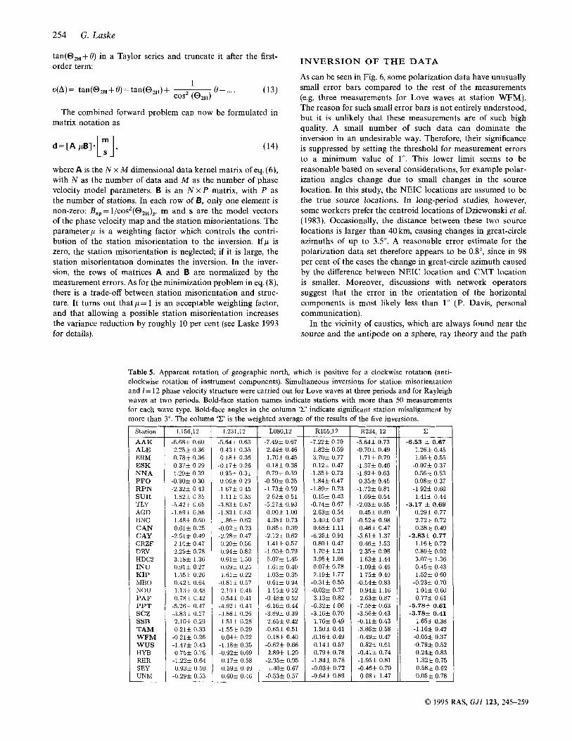
Table 5. Apparent rotation of geographic north, which is positive for a clockwise rotation (anti- clockwise rotation of instrument components). Simultaneous inversions for station misorientation and I = 12 phase velocity structure were carried out for Love waves at three periods and for Rayleigh waves at two periods. Bold-face station names indxate stations with more than 50 measurements for each wave type. Bold-face angles in the column 'Z' indicate significant station misalignment by more than 3". The column 'Z' is the weighted average of the results of the five inversions.

Station

AAK ALE ERM ESK NNA PFO RPN SUR TLY AGD BNG CAN CAY CRZF DRV HDCS INU KIP MBO NOU PAF PPT scz SSB TAM WFM wus HYB RER SEY UNM

L156.12

-6.68f 0.60 2.25f 0.36 0.781 0.36 0.37f 0.29 1.29f 0.39

-0.301 0.30 -2.32f 0.43 1.82% 0.35

-5.42+ 0.65 -1.691 0.86 1.48f 0.60 O.6lf 0.25

-2.51f 0.49 2.101 0.47 2.29+ 0.78 3.18f 1.36 0.91f 0.27 1.55f 0.26 0.42* 0.64 1.131 0.48 0.78& 0.42

-5.261 0.47 -3.831 0.27 2.10f 0.29 0 .2H 0.33

-0.21f 0.26 -1.473~ 0.43

-1.22f 0.64 0.93f 0.50

-0.2Yf 0.53

0 . m 0.76

L231,12

-5.64% 0.63 0.431 0.35 0.181 0.36

-0.17f 0.26 0.95% 0.31 0.06f 0.29

-1 67% 0.45 1.112c 0.38

-3.831 0.67 -1.83f 0.63 1.861 0.62

-0.02+ 0.23 -2.281 0.47 0.20f 0.56 0.94+ 0.82 0.61% 1.50 0.09% 0.25 1.61f 0.22

-0.811 0.57 2.10% 0.46 0.541 0.41

-4.92* 0.43 - 3 . 8 6 i 0.26 1.511 0.28

-1.55f 0.29 0.04f 0.22

-1.18f 0.35 -0.921 0.69 -0.17f 0.58 0S9f 0.49 K 6 0 i 0.46

L080,12

-7.49f 0.67 2.44f 0.46 1.701 0.45 0.181 0.38 0.79f 0.59

-0.50f 0.35 -1.73f 0.59 2.621 0.51

-5.27f 0.93 0.001 1.00 4.381 0.73 0.851 0.39

-2.121 0.62 1.41% 0.57

-1 90f 0.79 5.071 1.45 l .Gl1 0.40 1.03f 0.35 0.6lf 0.94 1.554~ 0.52

-0.48f 0.52 -6.16f 0.44 -3.891 0.39 2.65f 0.42

-0.65f 0.51 0.181 0.40

-0.62f 0.66 2.891 1.20

-2.95f 0.95 1.40f 0.67

-0.53f 0.57

R155,12

-7.22+ 0.70 1.821 0.59 3.70f 0.77 0.12f 0.47

-1.351 0.73 1.841 0.47

-1.891 0.73 0.15f 0.43

-0.74f 0.67 2.63f 0.54 5.40f 0.67 0.681 1.11

-6.25f 0.91 0.803~ 0.47 1.70f 1.21 3.951 1.06 0.07f 0.78 2.19f 1.77

-0.31f 0.50 -0.02f 0.37 3.13f 0.82

-6.32f 1.06 -3.16f 0.70 1.761 0.49

-1.50f 0.41 .0.16f 0.49 0.14f 0.57 0.79f 0.78

-1.84f 0.78 -0.03f 0.72 -0.64+ 0.89

R234. 12

-5.64f 0.73 -0.70f 0.49 1.71f 0.79

-1.37f 0.46 -1.82f 0.63 0.351 0.45

-1.72f 0.81 1.69f 0.54

-2.03f 0.55 0.455 0.80

-0.521 0.98 0.461 0.47

-5.61f 1.37 0.462~ 1.53 2.351 0.98 1.63f 1.44

-1.09f 0.46 1.75f 0.40

-0.54f 0.83 0.941 1.16 2.631 0.87

-7.58+ 0.63 -3.56f 0.43 -0.111 0.43 -3.861 0.58 -0.491 0.47 0.52f 0.61

-0.41f 0.74 -1.95f 0.81 -0.46f 0.70 0.08f 1.47

c -6.53 f 0.67

1.261 0.45 1.05f 0.55

-0.07f 0.37 0.561 0.53 0.081 0.37

-1.925 0.60 1.411 0.44

-3.17 f 0.69 0.29rt 0.77 2.723~ 0.72 0.38f 0.49

-2.83f 0.77 1.16f 0.72 0.891 0.92 3.071 1.36 0.452~ 0.43 1.5% 0.60

-0.231 0.70 1 .Olf 0.60 0.771 0.61

-5.7Szt2 0.61 -3.781 0.41

1.651t 0.38 -1.161t 0.42 -0.05f 0.37 -0.791 0.52 0.241 0.83

-1.321 0.75 0.581 0.62

-0.05k 0.78

0 1995 RAS, GJI 123, 245-259

Off-great-circle propagation 255

lov 156.16 ray 155 ray 169

integral approximation used in the inversion are no longer valid. Lateral heterogeneity can stretch these caustics to shorter epicentral distances so that the measured angles cannot be modelled with great reliability (Wang, Dahlen & Tromp 1993). To account for this, the data and the elements in the data kernel matrix are weighted by sin (A), where A is the epi- central distance.

As one might expect, due to the imperfect nature of our data set, a joint inversion for structure and station orientation could lead to rather different station orientations if data were used at only one period. In order to decrease uncertainties in the determination of instrument misalignment and bias in the final phase velocity maps, the inversion is performed in a two- step procedure. The first step involves the non-linear joint inversions for structure and station orientation for Love and Rayleigh waves at various periods. The resulting misalignment is averaged at each station and the data are corrected. The second step is the linear inversion of the corrected polarization data for the final phase velocity maps. The iterative joint inversions for phase velocity structure (up to 1=12) and component misalignment result in apparent rotations of geo- graphic north at 31 of the 37 stations. Misalignments at the six stations ECH, NOC, GAR, LVZ, NRIL and NVS are not considered further, as there are less than five measurements at these sites (NOU and NOC are considered to be different). The inversion converges quickly (after three iterations, appar- ent north does not change by more that 0.01"). This procedure is repeated for Love waves at three periods (T=231, 156 and 80s) and for Rayleigh waves at two periods (T=234, 155s; Table 5) . The weighted mean value of the resulting angles of the five inversions is considered to be the final apparent direction of geographic north, 8. At stations with a large amount of data, the inversion for 8 is relatively stable, so that 8 changes within the error bars for the five chosen periods. Significant clockwise misorientation of more than 3" can be found at stations AAK, TLY, PPT and SCZ. Since few measurements are available at TLY, the misorientation at this site should be considered carefully. The horizontal components at site CAY might be misaligned by 2" as well, although the inversion for Love waves reveals much smaller angles than for Rayleigh waves. Particularly at stations with relatively few measurements (e.g. BNG, HDC2, RER), apparent north can change significantly from inversion to inversion, and it seems that the formal error bars resulting from the inversion are too small. In these cases, the misorientations are probably deter- mined to within an accuracy of not better than 1.5". In the case of site AAK, the operators found a misalignment of the north component of 6". Although our inversion cannot detect this non-orthogonal orientation of the components, the tech- nique is obviously very helpful in identifying possible station

4715 2394 49.2 8.7 51520 1680 1.4 2521 1868 25.9 4.2 16692 1423 1.3 2466 1753 28.9 5.2 25340 1440 1.2

misalignments. At this point, it is important to note that both non-orthogonality of the three components and a poorly known instrument calibration could map into the rotation of apparent north.

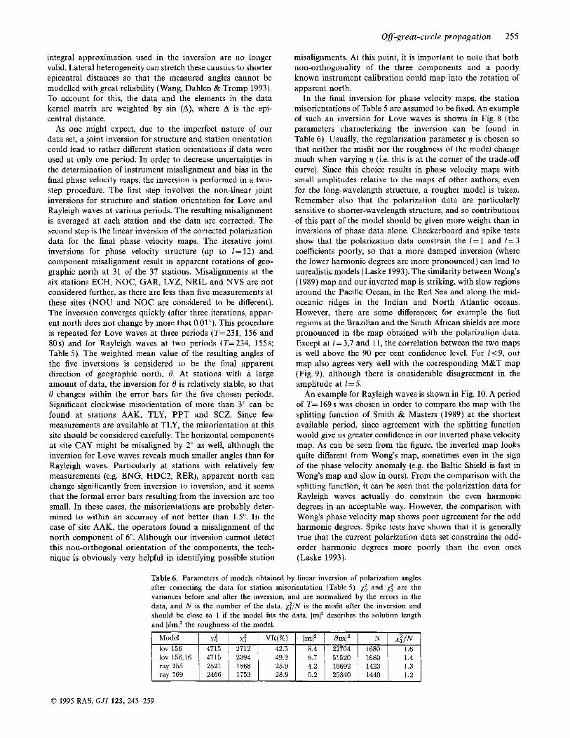
In the final inversion for phase velocity maps, the station misorientations of Table 5 are assumed to be fixed. An example of such an inversion for Love waves is shown in Fig. 8 (the parameters characterizing the inversion can be found in Table 6). Usually, the regularization parameter q is chosen so that neither the misfit nor the roughness of the model change much when varying q (i.e. this is at the corner of the trade-off curve). Since this choice results in phase velocity maps with small amplitudes relative to the maps of other authors, even for the long-wavelength structure, a rougher model is taken. Remember also that the polarization data are particularly sensitive to shorter-wavelength structure, and so contributions of this part of the model should be given more weight than in inversions of phase data alone. Checkerboard and spike tests show that the polarization data constrain the 1=1 and 1=3 coefficients poorly, so that a more damped inversion (where the lower harmonic degrees are more pronounced) can lead to unrealistic models (Laske 1993). The similarity between Wong's (1989) map and our inverted map is striking, with slow regions around the Pacific Ocean, in the Red Sea and along the mid- oceanic ridges in the Indian and North Atlantic oceans. However, there are some differences; for example the fast regions at the Brazilian and the South African shields are more pronounced in the map obtained with the polarization data. Except at 1 = 3,7 and 11, the correlation between the two maps is well above the 90 per cent confidence level. For 159, our map also agrees very well with the corresponding M&T map (Fig. 9), although there is considerable disagreement in the amplitude at 1 = 5.

An example for Rayleigh waves is shown in Fig. 10. A period of T= 169 s was chosen in order to compare the map with the splitting function of Smith & Masters (1989) at the shortest available period, since agreement with the splitting function would give us greater confidence in our inverted phase velocity map. As can be seen from the figure, the inverted map looks quite different from Wong's map, sometimes even in the sign of the phase velocity anomaly (e.g. the Baltic Shield is fast in Wong's map and slow in ours). From the comparison with the splitting function, it can be seen that the polarization data for Rayleigh waves actually do constrain the even harmonic degrees in an acceptable way. However, the comparison with Wong's phase velocity map shows poor agreement for the odd harmonic degrees. Spike tests have shown that it is generally true that the current polarization data set constrains the odd- order harmonic degrees more poorly than the even ones (Laske 1993).

Table 6. Parameters of models obtained by linear inversion of polarization angles after correcting the data for station misorientation (Table 5) . ,Y; and ,Y: are the variances before and after the inversion, and are normalized by the errors in the data, and N is the number of the data. ,y:/N is the misfit after the inversion and should be close to 1 if the model fits the data. [mlZ describes the solution length and ldrn1' the roughness of the model.

0 1995 RAS, G J I 123, 245-259

256 G. Laske

1=12, 1156

lov. 156

(0 .-

60

15000 30000 roughness

lov.156 Wong-new

3

1.5

0

-1.5

-3

P o l a r i z a t i o n

0.8 99 9 5

c 0.4 90

- 0.0 ??

-0.4

0

0

.- 4

I 0

-0.8

2 4 6 8 10 12

I

I * . O T

3

1.5

0

-1.5

-3

I I I I I 12

0.00' I 2 4 6 8 10

(c> Harmonic degree

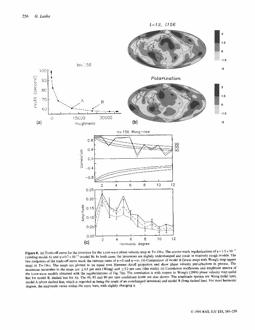
Figure 8. (a) Trade-off curve for the inversion for the Love-wave phase velocity map at T= 156s. The arrows mark regularizations of q = 1.5 x lo-' (yielding model A) and q=0.7 x (model B). In both cases, the inversions are slightly underdamped and result in relatively rough models. The two endpoints of the trade-off curve mark the extreme cases of q = O and q+m. (b) Comparison of model B (lower map) with Wong's map (upper map) at T=156s. The maps are plotted in an equal area Hammer-Aitoff projection and show phase velocity perturbations in percent. The maximum anomalies in the maps are f4.5 per cent (Wong) and k3.2 per cent (this study). (c) Correlation coefficients and amplitude spectra of the Love-wave models obtained with the regularizations of Fig. 7(a). The correlation is with respect to Wong's (1989) phase velocity map (solid line for model B, dashed line for A). The 99, 95 and 90 per cent confidence levels are also shown. The amplitude spectra are Wong (solid line), model A (short dashed line, which is regarded as being the result of an overdamped inversion) and model B (long dashed line). For most harmonic degrees, the amplitude varies within the error bars, with slightly changing q.

'

0 1995 RAS, GJI 123,245-259

Of-grea t -c irc le propagation 2 5 7

lov.156 Mont - new12,16

2 4 6 8 10 12 14 16 0.25

0 05

000’ 1 1

2 4 6 8 10 12 14 16 Harmonic degree

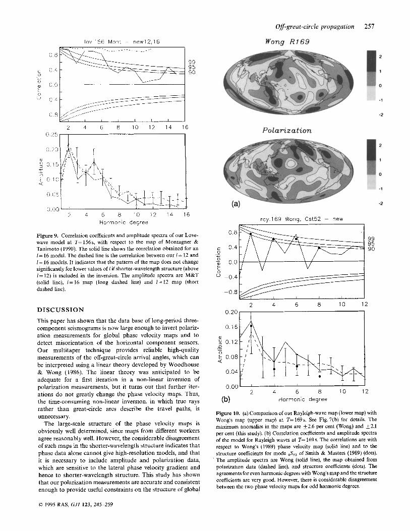
Figure 9. Correlation coefficients and amplitude spectra of our Love- wave model at T= 156 s, with respect to the map of Montagner & Tanimoto (1990). The solid line shows the correlation obtained for an I = 16 model. The dashed line is the correlation between our I = 12 and 1= 16 models. It indicates that the pattern of the map does not change significantly for lower values of 1 if shorter-wavelength structure (above I = 12) is included in the inversion. The amplitude spectra are M&T (solid line), 1=16 map (long dashed line) and 1=12 map (short dashed line).

DISCUSSION

This paper has shown that the data base of long-period three- component seismograms is now large enough to invert polariz- ation measurements for global phase velocity maps and to detect misorientation of the horizontal component sensors. Our multitaper technique provides reliable high-quality measurements of the off-great-circle arrival angles, which can be interpreted using a linear theory developed by Woodhouse & Wong (1986). The linear theory was anticipated to be adequate for a first iteration in a non-linear inversion of polarization measurements, but it turns out that further iter- ations do not greatly change the phase velocity maps. Thus, the time-consuming non-linear inversion, in which true rays rather than great-circle arcs describe the travel paths, is unnecessary.

The large-scale structure of the phase velocity maps is obviously well determined, since maps from different workers agree reasonably well. However, the considerable disagreement of such maps in the shorter-wavelength structure indicates that phase data alone cannot give high-resolution models, and that it is necessary to include amplitude and polarization data, which are sensitive to the lateral phase velocity gradient and hence to shorter-wavelength structure. This study has shown that our polarization measurements are accurate and consistent enough to provide useful constraints on the structure of global

ray.169 Wonq, Cst52 - new

0.8 99 95

c 0.4 90

- 0.0 2

0

0 .- c

L n

-0.4

-0.8

2 4 6 8 10 12 0.20

-

e, ; 0.12 - I \ c

- 1 \

-,’ - .- - a

- - _ E 0.08 Q

0.04

‘

0.001 I I I I I I 2 4 6 8 10 12

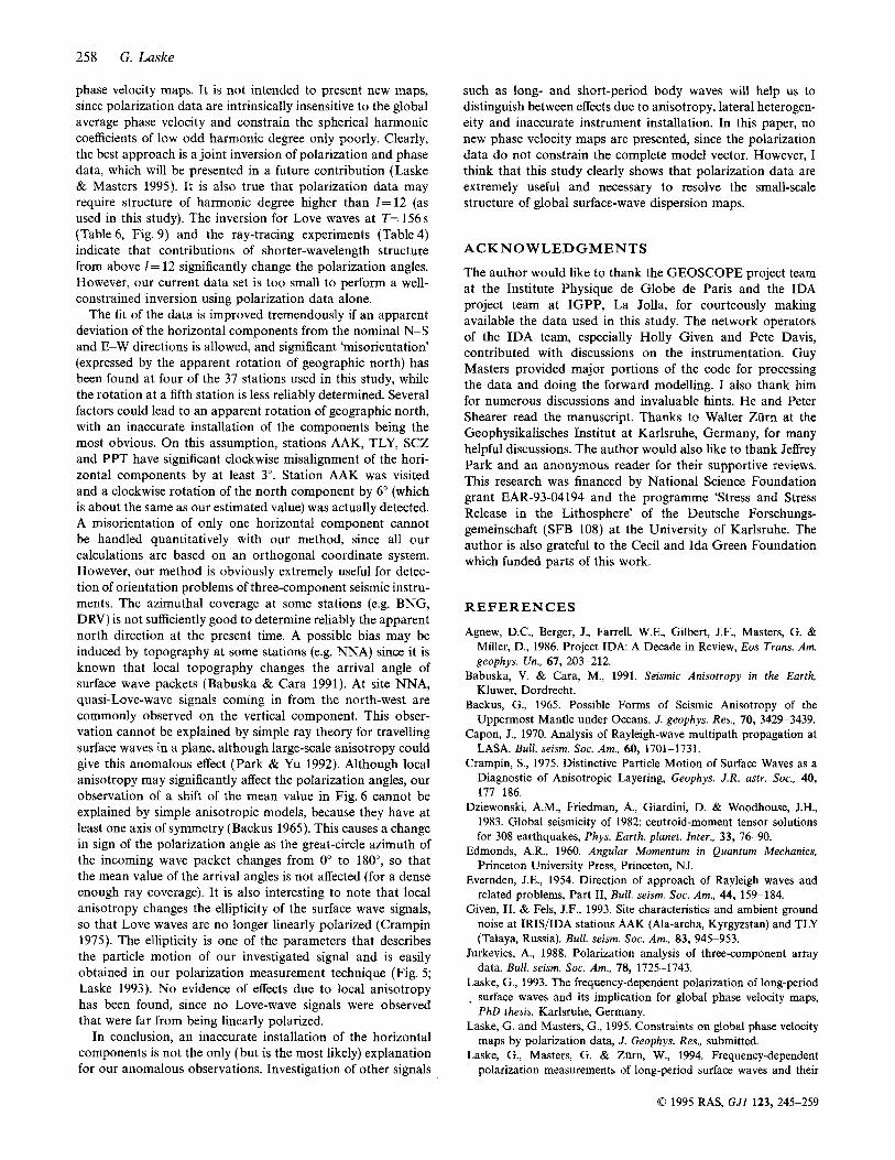
Harmonic degree (b) Figure 10. (a) Comparison of our Rayleigh-wave map (lower map) with Wong’s map (upper map) at T=169s. See Fig. 7(b) for details. The maximum anomalies in the maps are k2.6 per cent (Wong) and k2.1 per cent (this study). (b) Correlation coefficients and amplitude spectra of the model for Rayleigh waves at T= 169 s. The correlations are with respect to Wong’s (1989) phase velocity map (solid line) and to the structure coefficients for mode $,, of Smith & Masters (1989) (dots). The amplitude spectra are Wong (solid line), the map obtained from polarization data (dashed line), and structure coefficients (dots). The agreements for even harmonic degrees with Wong’s map and the structure coefficients are very good. However, there is considerable disagreement between the two phase velocity maps for odd harmonic degrees.

0 1995 RAS, GJI 123, 245-259

250 G. Laske

phase velocity maps. It is not intended to present new maps, since polarization data are intrinsically insensitive to the global average phase velocity and constrain the spherical harmonic coefficients of low odd harmonic degree only poorly. Clearly, the best approach is a joint inversion of polarization and phase data, which will be presented in a future contribution (Laske & Masters 1995). It is also true that polarization data may require structure of harmonic degree higher than I = 12 (as used in this study). The inversion for Love waves at T= 156 s (Table 6, Fig. 9) and the ray-tracing experiments (Table 4) indicate that contributions of shorter-wavelength structure from above J = 12 significantly change the polarization angles. However, our current data set is too small to perform a well- constrained inversion using polarization data alone.

The fit of the data is improved tremendously if an apparent deviation of the horizontal components from the nominal N-S and E-W directions is allowed, and significant 'misorientation' (expressed by the apparent rotation of geographic north) has been found at four of the 37 stations used in this study, while the rotation at a fifth station is less reliably determined. Several factors could lead to an apparent rotation of geographic north, with an inaccurate installation of the components being the most obvious. On this assumption, stations AAK, TLY, SCZ and PPT have significant clockwise misalignment of the hori- zontal components by at least 3". Station AAK was visited and a clockwise rotation of the north component by 6" (which is about the same as our estimated value) was actually detected. A misorientation of only one horizontal component cannot be handled quantitatively with our method, since all our calculations are based on an orthogonal coordinate system. However, our method is obviously extremely useful for detec- tion of orientation problems of three-component seismic instru- ments. The azimuthal coverage at some stations (e.g. BNG, DRV) is not sufficiently good to determine reliably the apparent north direction at the present time. A possible bias may be induced by topography at some stations (e.g. NNA) since it is known that local topography changes the arrival angle of surface wave packets (Babuska & Cara 1991). At site NNA, quasi-Love-wave signals coming in from the north-west are commonly observed on the vertical component. This obser- vation cannot be explained by simple ray theory for travelling surface waves in a plane, although large-scale anisotropy could give this anomalous effect (Park & Yu 1992). Although local anisotropy may significantly affect the polarization angles, our observation of a shift of the mean value in Fig. 6 cannot be explained by simple anisotropic models, because they have at least one axis of symmetry (Backus 1965). This causes a change in sign of the polarization angle as the great-circle azimuth of the incoming wave packet changes from 0" to 180°, so that the mean value of the arrival angles is not affected (for a dense enough ray coverage). It is also interesting to note that local anisotropy changes the ellipticity of the surface wave signals, so that Love waves are no longer linearly polarized (Crampin 1975). The ellipticity is one of the parameters that describes the particle motion of our investigated signal and is easily obtained in our polarization measurement technique (Fig. 5; Laske 1993). No evidence of effects due to local anisotropy has been found, since no Love-wave signals were observed that were far from being linearly polarized.

In conclusion, an inaccurate installation of the horizontal components is not the only (but is the most likely) explanation for our anomalous observations. Investigation of other signals

such as long- and short-period body waves will help us to distinguish between effects due to anisotropy, lateral heterogen- eity and inaccurate instrument installation. In this paper, no new phase velocity maps are presented, since the polarization data do not constrain the complete model vector. However, I think that this study clearly shows that polarization data are extremely useful and necessary to resolve the small-scale structure of global surface-wave dispersion maps.

ACKNOWLEDGMENTS

The author would like to thank the GEOSCOPE project team at the Institute Physique de Globe de Paris and the IDA project team at IGPP, La Jolla, for courteously making available the data used in this study. The network operators of the IDA team, especially Holly Given and Pete Davis, contributed with discussions on the instrumentation. Guy Masters provided major portions of the code for processing the data and doing the forward modelling. I also thank him for numerous discussions and invaluable hints. He and Peter Shearer read the manuscript. Thanks to Walter Zurn at the Geophysikalisches Institut at Karlsruhe, Germany, for many helpful discussions. The author would also like to thank Jeffrey Park and an anonymous reader for their supportive reviews. This research was financed by National Science Foundation grant EAR-93-04194 and the programme 'Stress and Stress Release in the Lithosphere' of the Deutsche Forschungs- gemeinschaft (SFB 108) at the University of Karlsruhe. The author is also grateful to the Cecil and Ida Green Foundation which funded parts of this work.

REFERENCES

Agnew, D.C., Berger, J., Farrell, W.E., Gilbert, J.F., Masters, G. & Miller, D., 1986. Project IDA A Decade in Review, Eos Trans. Am. geophys. Un., 67 , 203-212.

Babuska, V. & Cara, M., 1991. Seismic Anisotropy in the Earth, Kluwer, Dordrecht.

Backus, G., 1965. Possible Forms of Seismic Anisotropy of the Uppermost Mantle under Oceans. J. geophys. Res., 70, 3429-3439.

Capon, J., 1970. Analysis of Rayleigh-wave multipath propagation at LASA. Bull. seism. SOC. Am., 60, 1701-1731.

Crampin, S., 1975. Distinctive Particle Motion of Surface Waves as a Diagnostic of Anisotropic Layering, Geophys. J.R. astr. SOC., 40, 177-1236,

Dziewonski, A.M., Friedman, A., Giardini, D. & Woodhouse, J.H., 1983. Global seismicity of 1982: centroid-moment tensor solutions for 308 earthquakes, Phys. Earth. planet. Inter., 33 , 76-90.

Edmonds, A.R., 1960. Angular Momentum in Quantum Mechanics, Princeton University Press, Princeton, NJ.

Evernden, J.E., 1954. Direction of approach of Rayleigh waves and related problems, Part 11, Bull. seism. SOC. Am., 44, 159-184.

Given, H. & Fels, J.F., 1993. Site characteristics and ambient ground noise at IRIS/IDA stations AAK (Ala-archa, Kyrgyzstan) and TLY (Talaya, Russia). Bull. seism. SOC. Am., 83, 945-953.

Jurkevics, A., 1988. Polarization analysis of three-component array data. Bull. seism. SOC. Am., 7 8 , 1725-1743.

Laske, G., 1993. The frequency-dependent polarization of long-period " surface waves and its implication for global phase velocity maps,

PhD thesis, Karlsruhe, Germany. Laske, G. and Masters, G., 1995. Constraints on global phase velocity

maps by polarization data, J. Geophys. Res., submitted. Laske, G., Masters, G. & Zurn, W., 1994. Frequency-dependent

polarization measurements of long-period surface waves and their

0 1995 RAS, GJI 123, 245-259

Off-great-circle propagation 259

implications for global phase-velocity maps, Phys. Earth. planet. Inter., 84, 111-137.

Lay, T. & Kanamori, H., 1985. Geometric effects of global lateral heterogeneity on long-period surface wave propagation, J. geophys. Res., 90, 605-622.

Lerner-Lam, A.L. & Park, J.J., 1989. Frequency-dependent refraction and multipathing of 10-100 second surface waves in the Western Pacific, Geophys. Res. Lett., 16, 527-530.

Masters, G., Priestley, K.F. & Gilbert, F., 1984. Observations of off- path propagation on horizontal component low frequency seismo- grams, Terra Cognita, 4, 250.

Montagner, J.-P. & Tanimoto, T., 1990. Global anisotropy in the upper mantle inferred from the regionalization of phase velocities, J. geophys. Res., 95, 4797-4819 (M&T).

Park, J., 1989. Roughness constraints in surface wave tomography. Geophys. Res. Let., 16, 1329-1332.

Park, J., Vernon 111, F.L. & Lindberg, C.R., 1987a. Frequency depen- dent polarization analysis of high-frequency seismograms, J. geophys. Rex, 92, 12 664-12 674.

Park, J., Lindberg, C.R. & Vernon 111, F.L., 1987b. Multitaper spectral analysis of high-frequency seismograms, J. geophys. Res., 92,

Park, J. & Yu, Y., 1992. Anisotropy and coupled free oscillations: simplified models and surface wave observations, Geophys. J. Int.. 110, 401-420.

Paulssen, H., Levshin, A.L., Lander, A.V. & Snieder, R., 1990. Time- and frequency-dependent polarization analysis: anomalous surface wave observations in Iberia, Geophys. J. Int., 103,483-496.

Press, W.H., Flannery, B.P., Teukolsky, S.A. & Vetterling, W.T., 1992. Numerical Recipes, The Art of Scient$c Computing, Cambridge University Press, Cambridge.

Romanowicz, B., Cara, M., Fels, J.F. & Roult, G., 1984. GEOSCOPE A French initiative in long period three component global seismic networks. EOS Trans. Am. geophys. Un., 65, 753-756.

Schwartz, S.Y. & Lay, T., 1987. Effects of off great-circle propagation on the phase of long-period surface waves, Geophys. J. R . astr. SOC.,

12 675-12684.

91, 143-154.

Slepian, D., 1978. Prolate spheroidal wave functions, Fourier analysis, and uncertainty. V The discrete case, Bell Systems Tech. J., 57,

Smith, M.F. & Masters, G., 1989. Aspherical Structure Constraints From Free Oscillation Frequency and Attenuation Measurements, J . geophys. Res., 94, 1953-1976.

Sobel, P.A. & von Seggern, D.H., 1978. Applications of surface-wave ray tracing, Bull. seism. SOC. Am., 68, 1359-1380.

Su, W. & Dziewonski, A.M., 1991. Predominance of long-wavelength heterogeneity in the mantle, Nature, 352, 121-126.

Taylor, J.R., 1982. An Introduction to Error Analysis, University Science Books, Mill Valley, CA.

Vidale, J.E., 1986. Complex polarization analysis of particle motion, Bull. seism. SOC. Am., 76, 1393-1405.

Wang, Z., Dahlen, F.A. & Tromp, J., 1993. Surface wave caustics, Geophys. J. Int., 114, 311-324.

Widmer, R., 1991. The Large-Scale Structure of the Deep Earth as Constrained by Free oscillation Observations, PhD thesis, University of California San Diego, Scripps Institution of Oceanography, San Diego.

Wong, Y.K., 1989. Upper mantle heterogeneity from phase and ampli- tude data of mantle waves, PhD thesis, Harvard University, Cambridge.

Woodhouse, J.H. & Dahlen, F.A., 1978. The effect of a general aspherical perturbation on the free oscillations of the Earth, Geophys. J . R. astr. SOC., 53, 335-354.

Woodhouse, J.H. & Wong, Y.K., 1986. Amplitude, phase and path anomalies of mantle waves, Geophys. J . R. astr. SOC., 87, 753-773.

Woodward, R.L. & Masters, G., 1992. Upper mantle structure from long-period differential traveltimes and free oscillation data, Geophys. J. Int., 109, 275-293.

Yu, Y. & Park, J., 1993. Upper mantle anisotropy and coupled-mode long-period surface waves, Geophys. J. Int., 114, 473489.

Zhang, Y.4 . & Tanimoto, T., 1993. High-Resolution global Upper Mantle Structure and Plate Tectonics, J. geophys. Res., 98,

1371-1430.

9793-9823 (Z&T).

0 1995 RAS, GJI 123, 245-259