Embed Size (px)
Citation preview

Global Monetary Conditions versus Country-Specific Factors in the Determination
of Emerging Market Debt Spreads
By
Mansoor Dailami1, Paul R. Masson2, and
Jean Jose Padou3
May, 2005
1 World Bank, Development and Prospects Group. The findings, interpretations, and conclusions expressed in this paper are entirely those of the authors. They do not necessarily represent the views of the World Bank, its Executive Directors, or the countries they represent.2 Rotman School of Management, University of Toronto3 University of Toronto
2
Global Monetary Conditions versus Country-Specific Factors in the Determination of Emerging Market Debt Spreads
By
Mansoor Dailami4, Paul R. Masson5, and
Jean Jose Padou6
May, 2005
Abstract
We offer evidence in this paper that US interest rate policy has an important
influence in the determination of credit spreads on emerging market bonds over US
benchmark treasuries, and therefore on their cost of capital. Our analysis improves upon
the existing literature and understanding, by addressing the dynamics of market
expectations in shaping views on interest rate and monetary policy changes, and by
recognizing non-linearities in the link between US interest rates and emerging market
bond spreads, as the level of interest rates affects the market's perceived probability of
default and the solvency of emerging market borrowers. For a country with a moderate
level of debt, repayment prospects would remain good in the face of an increase in US
interest rates, so there would be little increase in spreads. A country close to the
borderline of solvency would face a steeper increase in the spreads. Simulations of a 200
basis points (bps) increase in US short-term interest rates (ignoring any change in the US
10 year Treasury rate) show an increase in emerging market spreads ranging from 6 bps
to 65 bps, depending on debt/GDP ratios.
4 World Bank, Development and Prospects Group. The findings, interpretations, and conclusions expressed in this paper are entirely those of the authors. They do not necessarily represent the views of the World Bank, its Executive Directors, or the countries they represent.5 Rotman School of Management, University of Toronto6 University of Toronto

3
I. Introduction
How interest rate policies in major industrial countries affect the pricing of
emerging market debt remains an unresolved issue. Despite its very important policy and
practical implications, our understanding of this link is shaped more by episodic evidence
--in 1991, 1994, and 2003 when sharp swings in emerging market spreads coincided with
a cyclical shift in the stance of US monetary policy --than by rigorous research and
robust empirical findings. One point of view, popularized by the financial press,
emphasizes the role of investors’ risk tolerance or risk appetite, even though such factors
are likely driven by a host of global macroeconomic conditions and uncertainties,
including potentially the pace of changes in US interest rates, and are more directly
relevant to the equity market than fixed income bond markets. And, while considerable
literature exists on the determinants of emerging market debt spreads over US treasury
securities, that literature is disappointingly inconclusive concerning the effects of the
global interest rate environment. For instance, Arora and Cerisola (2000), Min et al.
(2003) and Ferrucci et al. (2004) find that the level of US interest rates plays a
considerable role in the determination of EM bond spreads--spreads widen as US rates go
up--but Kamin and von Kleist (1999) argue that there is little explanatory power of
industrial country short-term interest rates, once one controls for credit quality.
Eichengreen and Mody (2000), in contrast with all of the above, find that syndicated bank
loans to EM countries tend to respond positively to increases in US interest rates, and the
spread on those loans responds negatively—though this surprising result is very sensitive
to regional differences. Furthermore, studies focusing on the US corporate bond market
have also found a negative relationship between credit spreads and US Treasury yields

4
(Longstaff and Schwartz, 1995; Duffee, 1996, and 1998; Colin-Dufresne, Goldstein, and
Martin, 2001)7, as predicted by structural models of credit risk following Merton (1974).
Existing studies of the link between US interest rates and EM bond market
spreads have several weaknesses. One major shortcoming is the scant attention paid to
the dynamics of market expectations in shaping views on interest rate and monetary
policy changes, and how such policy changes are factored into the determination of bond
market prices and yields8. The hypothesis advanced here is that the market anticipates
the future behavior of the Fed by observing the evolution of relevant leading short-term
macroeconomic indicators and factors in such expectations well in advance of actual
changes in interest rates. This dynamic induces an important correlation between EM
bond spreads and key indicators of the US economic outlook such as the US non-farm
payrolls report and retail sales, as is clearly demonstrated by recent experience--much of
the market reaction regarding the EM bond spreads occurred in April/May 2004, when
the reported payroll figures indicated stronger growth momentum than anticipated by the
market9. The reason for this dynamic is the particular institutional setting of interest rates
in the US, where under the prevailing regime (which in many ways is equivalent to
inflation targeting, without an explicit target), the market comes to form views about Fed
7
Also studies by Leake (2003), and Boss and Scheicher (2002) focusing respectively on the UK and Euro-corporate bond markets, find a small negative relationship between credit spreads on sterling investment-grade corporate bonds and the level and slope of the term structure of UK interest rates.8 Arora and Cerisola (2000) however look at the predictability of US monetary policy, and find that heightened uncertainty about that policy leads to a widening of spreads.9 As Uribe and Yue (2003) note, US interest rates also help to drive business cycles in EM economies, and spreads respond to EM activity. However, their empirical results show that US interest rate shocks affect domestic EM variables mostly through their effects on country spreads.
5
behavior, based on the evolution of certain leading short-term economic indicators, such
as payroll figures, retail sales, and core inflation data10.
A second weakness of the existing literature is the lack of attention paid to the
non-linearity in the relationship between US interest rates and EM spreads. Indeed, the
spread incorporates a default probability in a non-linear way, and the effect of higher
world interest rates itself affects the default probability non-linearly. For instance, at low
rates of interest and in periods of favorable economic activity and low debt in developing
countries, a rise in US interest rates may have little effect on investors’ estimates of the
probability of repaying—and indeed, on the objective likelihood of that repayment. In
contrast, when the EM borrower is at the borderline of its ability to repay, a given
increase in US rates may push the borrower over the edge, sharply increasing the
probability of default. Such a scenario may have occurred, for instance, in 1982 and
1994.
A further aspect of that non-linearity is that sharp shifts of expectations of default
probabilities may be self-fulfilling, and correspond to jumps between multiple equilibria.
Indeed, those expectations can be rational because higher interest rates will increase the
likelihood that countries cannot meet their debt service obligations. While models with
sunspot equilibria are sometimes criticized as just adding an extra indeterminacy because
what triggers the jumps between equilibria is not explained, in international capital
markets, that role may be assumed by global liquidity conditions and the “appetite for
risk.” In our estimation, we divide the sample into crisis and non-crisis periods. We also
10 This accords with the view and assessment of key market practitioners. A credit market strategist was quoted by Credit (2004) as saying, “it is not the rate hikes that matter, but what is happening to the economy”.

6
include proxies for international liquidity and for contagion in financial markets. Indeed,
given that there are investors in EM bonds that are common across countries, it is natural
to expect that a crisis in one country should be associated with higher spreads in other
markets, if they both are the result of a changed attitude to risk or liquidity.
A third improvement relative to the current literature is our use of more recent
data (until June, 2004)—and longer time series; this may help to distinguish between
hypotheses. In particular, we use monthly data for individual country Emerging Market
Bond Index Plus (EMBI+) spreads, available from JP Morgan which is a major dealer in
emerging bond markets, and extending back for some countries to 1991. The bonds are
issued in US dollars, so that spreads reflect credit risk—the probability that the borrower
will not repay. The set of countries includes all the major sovereign borrowers, and the
data are based on trading in secondary markets of Brady bonds and Eurodollar issues.
Our sample includes the following 17 countries: Argentina, Brazil, Bulgaria, Colombia,
Ecuador, Mexico, Morocco, Nigeria, Panama, Peru, the Philippines, Poland, Russia,
South Africa, Turkey, Ukraine, and Venezuela. We estimate an unbalanced panel, with
data availability varying from country to country. While the data on spreads are based on
secondary market data, they provide many more data points and allow a finer
appreciation of the effects of interest rate increases than primary market data. Moreover
with transaction volumes in secondary markets surpassing those in primary markets by
several fold, spreads based on secondary market prices are more informative and less
contaminated by supply effects than the spreads for new issues.

7
II. A Framework for Analysis
Our approach to understanding the link between US interest rates and emerging
market debt spreads focuses on the impact of interest rates on the market’s perceived
probability of default. The starting point here is the simple relationship between the
probability of default p on EM bonds and the rate of interest on riskless securities, say US
treasuries, paying rate, r (see, for instance, Arora and Cerisola, 2000). If the default is
complete (with no repayment of either principal or interest11) , investors are risk neutral,
and assuming away the possibility of default correlation across borrowers, then the
interest rate i on EM bonds should yield the same expected return as US treasuries, so
0)1)(1(1 ppir (1)
Therefore, the spread S over US treasuries can be written
p
prriS
1)1( (2)
or, in log form,
(2’)
11 In studies where default is taken to be less than complete, the rate of recovery upon default is generally
assumed to be constant (see for instance, Elton et al. 2001).A constant recovery rate does not change our main results.
p
prS
1log)1log(log

8
We go behind this simple relationship to look at the determinants of the
ability to service the debt12, while leaving aside issues of voluntary default. Suppose that
the EM sovereign borrower has a stochastic income stream Y, and that it defaults when
that income is less than the debt service. Then the probability of default will be given by
])1
)1((Pr[]Pr[ Dp
prrYiDYp
(3)
We will further assume for concreteness that Y is determined by a first order
autoregression 1YY with innovations that are i.i.d. with distribution function F().
Let 1 YrDZ be the interest burden at a zero default probability minus expected
income. Then the probability of default can be written
]1
)1([]1
)1(Pr[ Dp
prZFD
p
prZp
(4)
It is important to note three things about the above equation: i) the probability
depends on the stock of debt, as well as lagged income; ii) equation (4) is highly non-
linear in the default probability; and iii) it can have multiple solutions, since, in general,
the right hand side is increasing in the default probability13. Figure 1 shows the case
where there are 3 intersections of the 45 degree line (the LHS of eq. 4) and the RHS of
the equation.
12 A seminal article is Eaton and Gersovitz (1981).13 See Jeanne (1997).

9

10
Figure 1. Multiple Solutions for Default Probabilities
p
p
The intuition is clear: by expecting a default, investors can make a default more
likely. However, this is only true in certain ranges for the variables and the parameters.
The “fundamental” variable Z needs to be in a certain range, and, in particular, debt D
has to be large enough that increases in interest costs can make debt service painful for
the EM borrower. A necessary condition for three solutions is that the cumulative
distribution function should have a slope greater than unity at some point—in particular,
at the middle intersection. Since the slope of this curve is simply the probability density
function f(x)=F’(x), it is straightforward to show that this condition requires that
1)1(
1]
1)1([
2
Dp
rD
p
prZf (5)
at the middle intersection point.
What is the effect of increasing the US interest rate on the probability of default?
Increasing the US rate shifts up the curve that corresponds to the RHS of (4): it increases
F[Z+(1+r)pD/(1-p)]

11
the value of p corresponding to the leftmost and the rightmost intersections—that is,
increases the default probabilities. It has the opposite effect on the middle intersection,
but, as in most models, that intersection is unstable, so it can be ignored. In addition to
increasing the value of p at the intersection points, it may also eliminate the two leftmost
intersections, leaving only the third one, with the highest probability of default. Thus, if
it shifts the curve up enough it may have a dramatic effect on the (rationally expected)
occurrence of default, since the upper equilibrium makes a default very likely.
Let us then examine how increases in the US interest rate would affect the spread.
From (2’),
dr
dp
pprdr
Sd
)1(
1
1
1log
(6)
We see that, since dp/dr>0, both terms on the right hand side of (6) are positive, so that
increases in US rates increase the spread. In addition to the non-linearity embodied in
dp/dr, the derivative dlogS/dr is also highly non-linear in p. A given change in the
probability of default dp/dr will have a larger effect on the spread when probabilities of
default are either very low or high than when they are close to one-half.
The implications of the above for developing a more rigorous estimation
methodology are two-fold. First, it is not sufficient just to include the US interest rate in
a linear regression explaining the spread. The effect on the spread is non-linear, and
depends on other variables. The time series of correlations of EMBI spreads with US
interest rates (measured over 36 month rolling periods between December 1992 and June
2004 ) show a great deal of fluctuation, with a clear break between crisis and non-crisis
periods (Figures 2 and 3).Thus interacting US interest rate variables with variables which

12
capture the severity of the debt problem may be essential to capturing the effect of global
monetary conditions on EM spreads.
Figure 2. Correlation of EMBI and US interest rates rolling three-yearperiods. Dec 1995-Aug 2004
-0.8
-0.6
-0.4
-0.2
0
0.2
0.4
0.6
0.8
1
Dec-95
Jun-96
Dec-96
Jun-97
Dec-97
Jun-98
Dec-98
Jun-99
Dec-99
Jun-00
Dec-00
Jun-01
Dec-01
Jun-02
Dec-02
Jun-03
Dec-03
Jun-04
fedrate
gs10
Figure 3 Correlation of EMBI and US interest rates rollingthree-year periods Dec 1995-Aug 2004
-1-0.8-0.6-0.4-0.2
00.20.40.60.8
1
Dec-95
Apr-96
Aug-96
Dec-96
Apr-97
Aug-97
Dec-97
Apr-98
Aug-98
Dec-98
Apr-99
Aug-99
Dec-99
Apr-00
Aug-00
Dec-00
Apr-01
Aug-01
Dec-01
Apr-02
Aug-02
Dec-02
Apr-03
Aug-03
Dec-03
Apr-04
Aug-04
fedrate
tb3m
Second, the possibility of multiple equilibria should be taken into account. We
see this possibility as being related to changes in global liquidity conditions and the
appetite for risk, and hence we introduce variables that attempt to capture those features
in regressions explaining the spreads. In addition, it may well be the case that the effect

13
of explanatory variables on the spreads is different, depending on which equilibrium is
chosen. Thus, it may make sense to divide the sample into two sub-samples: “normal”
times, and “crisis” periods when a particular country faces sharply higher spreads as a
result of a debt default or currency attack. For instance, it seems plausible that if a
country is in crisis, then the effect of world monetary conditions on the spread will be
less significant. It is likely that the country can emerge from crisis and reduce the very
high interest rates that it faces mainly by its own actions—unless the crisis was provoked
by a shift in global risk appetite (see next paragraph). In normal times, however,
countries’ spreads may be very sensitive to the conditions in global capital markets,
especially if they are in a middle region of high but not overwhelming debt. Dividing the
sample would prevent outliers from distorting estimates of the influence of “push”
factors. The occurrences of very high spreads in our sample are mostly associated with
defaults or currency crises on the part of the borrowing country: Mexico in December
1994, Russia in August 1998, and Argentina in February 2002, for instance.
Moreover, the existence of multiple equilibria gives a natural role to contagion
effects in international capital markets14. Again, this contagion may operate through a
change in global risk appetite, and in our model, be signaled by changes in the spread
between US corporate borrowers with high and low risk. It may also be evidenced by a
positive effect of the spread in non-crisis countries of a dummy variable that counts the
number of other countries in the crisis state. This could be expected to operate if the
14 For a discussion of the relationship between multiple equilibria and contagion, see Masson (1999; 2001). A contrary view of the relevance of multiple equilibria in financial markets is presented by Morris and Shin (1998; 2002). However, their argument relies on the iterated elimination of all dominated strategies (with infinite iteration), which experimental evidence suggests does not apply in real world situations (Camerer, 1997).

14
country itself is not in crisis; for the same reason as above, once a country is in the crisis
state it is mainly affected by its own variables—or, if the crisis was caused by a loss of
risk appetite, by an abatement of contagion and a return to more normal conditions.
III. Empirical Methodology
As in much of the empirical literature, we use panel regressions of the EM interest
rate spread over US treasuries on domestic determinants of a country’s credit-worthiness
as well as global variables that explain the supply and cost of credit to emerging markets.
Ferrucci et al. (2004) call the first set of variables “pull factors”, and the second, “push
factors”; their research concludes that both sets are important in explaining EM spreads.
However, as the discussion above suggests, it is difficult to separate the two sets of
variables conceptually. For instance, the level of US interest rates influences a country’s
creditworthiness since borrowing that is sustainable in a low world interest rate
environment (whatever the country’s economic fundamentals) may not be so when
interest rates are high.
We follow Ferrucci et al. (2004) in distinguishing between long run influences on
spreads, which are constrained to have the same coefficients for all countries, with the
short run dynamics that can vary from country to country and may include other
explanatory variables. The short-run dynamics are specified to take the form of an error
correction model, where the errors are deviations from the long-run equilibrium
relationship.
The econometrics behind this model in a panel context are described in Pesaran,
Shin, and Smith (1999). The model is estimated using their Pooled Mean Group
Estimator. In particular, we posit a long run relationship linking the log of spreads of EM

15
interest rates over comparable US treasuries, to US interest rates, the spread between high
and low risk US corporate bonds, and various variables reflecting the borrower’s
creditworthiness (trade openness, debt/income, the ratio of short-term debt in the total,
and reserves/debt). If we call all these right hand side variables the vector X, then the
long-run relationship is
(7)
where the intercept term may vary across countries, allowing for fixed effects, while the
slope coefficients are constrained to be the same. The dynamic equations take the form
error-correction models for which the short-run adjustment toward the same long-run
relationship can vary across countries:
(8)
The vector Y may include first differences of all or a subset of the X variables, plus
other variables that influence the short run dynamics but not the long-term equilibrium
level of spreads. In the latter category we include current changes in US monetary policy
variables and forecasts of their future evolution (to be described below).
Note that the estimation of (8) is not straightforward using panel estimation
programs, because of the non-linear constraints on the long run coefficients. In particular,
if we estimate
j
ijtjiit XS log
j
itiitijtjiiit YSXS ]log[log 11
j
iitiitiijtijiit uYdScXbS 1loglog

16
(9),
then we need to impose the following constraints
(10).
Estimation can be done in two stages, that is, first estimate the long term
regression, (7), and then use the lagged residuals to replace the term in square brackets in
(8). We use the two-stage approach for our exploratory regressions that aim to narrow
down the set of explanatory variables. However, this method is inefficient since it
ignores the effect of short-term dynamics when estimating the long-term coefficients β.
Therefore, the PMG estimates impose long-run coefficients in the context of a dynamic
panel regression.
When considering variables that may influence short-run dynamics, we include
changes in the above long-run determinants and also forecasts of the change in stance of
US monetary policy. Thus we first estimate forecasting equations for US interest rates
that include as explanatory variables lagged changes in US capacity utilization, retail
sales, the producer price index, and M2 data. Then we test whether these forecasts have
an additional effect, over and above the long run relationship between US interest rates
and EM spreads and the contemporaneous change in US rates.
In order to maximize the number of observations, and focus on the
macroeconomic determinants of US monetary policy, we estimate the model at a monthly
frequency, even if this limits the availability of country-specific determinants of EM
credit-worthiness. For many of the countries in our sample, data on consumer prices,
kjic
c
b
b
k
i
kj
ij ,,

17
reserves and the money supply are available monthly, while quarterly or annual data are
available for GDP and foreign debt. We interpolate the latter variables where necessary.
In specifying the effects of US monetary policy, we include in the long-run
relationship the levels of US short rates (the US Treasury bill rate15), the 10-year
Treasury bond rate, and the interest rate spread between high and low risk US corporate
bonds. The latter variables, as well as being influenced by US monetary policy, may also
capture global risk appetite. We interact the US T Bill rate with the country’s debt to
GNI ratio, since as discussed in section II, non-linearities are likely to be important.
We have argued that it is important to divide the sample into crisis and non-crisis
periods. A country i is in a non-crisis period t if in that period it is not suffering a crisis,
even if other countries are. But it is also possible that the existence of crises at t in other
countries—and their number—may increase the interest rate for country i. A significant
coefficient on the number of other countries in crisis may be evidence of contagion
effects, since, if positive, it would come over and above the country’s own fundamentals
and global monetary conditions.16
Dating of crisis periods is not straightforward, however. One approach is to let
the data on exchange market pressure (the sum of exchange rate changes and reserve
changes, appropriately weighted) identify crisis periods. A recent application is
Kaminsky (2003), and we use the crisis dates she identifies (Kaminsky, 2003, table 2),
but instead of assuming that the duration of each crisis is 24 months, we use a much
smaller window, six months following the crisis date in her list—except for Argentina.
15Arora and Cerisola (2000) suggest that the federal funds rate is more appropriate, but we find the TB rate to be a better explanatory variable of EM spreads.

18
In practice, the period of very high spreads has been limited to a few months, when a
resolution has been in sight. Argentina’s 2002 default is an exception, and we make the
crisis dummy continue to the end of our sample. We also add the Russian crisis, starting
in August 1998, since Russia is not in her sample.
IV. Estimation Results
We first describe the long-run (static) regressions of the log of spreads on both
push and pull factors. Of especial interest is the relative importance of the two sets, and
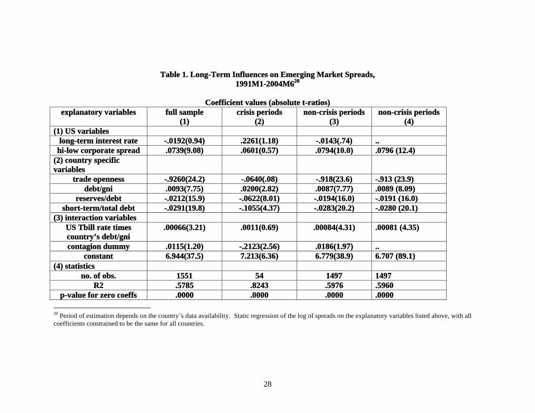
evidence of non-linearity in the relationship. Table 1 gives the coefficient estimates, with
the sample divided into crisis and non-crisis periods, with the latter dominating in our
sample (1497 months versus only 54 crisis periods17).
Country specific variables seem to dominate US interest rates in influence over
EM spreads. In particular, trade openness has a strong negative effect on spreads, which
is plausible since more open countries are better able to adjust their balance of payments
in order to generate earnings to service external debt; this variable may also reflect the
finding in the growth literature that more open countries tend to grow faster. As
expected, the level of debt to a country’s income has a significant positive influence on
the spread it faces, while the reserves/debt ratio and the proportion of short-term debt
both have a significant negative influence. The latter effect may simply reflect an
upward-sloping term structure.
16 Eichengreen, Rose and Wyplosz (1995) find that the occurrence of crises elsewhere tends to increase a country’s likelihood to experience a crisis.17 As noted above, our choice of a small crisis window (6 months) limits the number of crisis periods. In addition, our reliance on Kaminsky (2003) for the crisis dates no doubt misses some crises, since not all the countries in our sample are on her list.

19
Turning to the US interest rate variables, in non-crisis periods the US short-term
rate, entered linearly, did not have a significant coefficient (not reported), while the long-
term interest rate (reported here) has a negative, but insignificant, coefficient. These
results contrast with those of Ferrucci et al. (2004). However, the interest rate spread on
high-risk versus low-risk US corporate borrowers comes in very strongly in non-crisis
periods.
As we have argued above, the effect of US rates can be expected to be non-linear,
and the US treasury bill rate interacted with the borrowing country’s debt/gni ratio does
in fact enter significantly in non-crisis periods (column 3) and produces significantly
higher explanatory power than the interest rate entered alone. Thus, the impact of rising
US rates is higher, the higher is a country’s level of indebtedness. In non-crisis periods,
countries are also vulnerable to crises in other countries, as the contagion dummy (the
number of crises elsewhere) has a significant positive effect.
The relationship between global monetary conditions and the EM spread is quite
different during periods of crisis, as we can see from column 2 of the table. A chi-square
test rejects equality of the two sets of coefficients. In crisis periods the US Hi-low spread
and the US Tbill rate interacted with a country’s debt have no significant effect, as is also
the case for the US long rate (which was already true in non-crisis periods). In contrast,
all the “pull” factors except trade openness continue to have a significant influence on
EM spreads in the expected direction. Somewhat surprisingly, the contagion dummy
(that is, the number of other countries in crisis) has no longer a positive effect on
spreads—it is the reverse; conditioned on a country being in crisis, its spreads do not
suffer from other countries also being in crisis. Of course, the fact of being in a crisis
20
situation may itself depend on the contagion dummy. It is also true that the constant term
is significantly higher in column 2 than in column 3. In sum, it seems that interest rates
charged to crisis countries are more dependent on their own behavior than on conditions
on global capital markets.
When the crisis and non-crisis periods are pooled (column 1), not surprisingly the
estimates resemble those of column 3, given the preponderance of non-crisis
observations. However, the contagion dummy is now insignificant, and the explained
variance is lower than for either sub sample. Since equality of the two sets of coefficients
in the sub-samples is rejected, the usual procedure of estimating a combined sample of
crisis and non-crisis observations on spreads is not legitimate.
We then turn to the dynamic equations, which we estimate first by using the
residual from the long-run equations, in particular a somewhat more parsimonious model
reported in Table 1, column 4. The PMG technique is later used to estimate
unconstrained short run dynamics and a common long run relationship, but our initial
estimates, reported in Table 3, also constrain the short run dynamics to be the same. The
common short-run dynamics then give some idea of the average effect on spreads across
the set of EM countries.
Of particular interest to us is to see whether the forecasted stance of US monetary
policy, and not just current interest rate variables, helps explain the evolution of EM
spreads. Therefore, we first attempt to relate our US interest rate variables—the T Bill
rate, the 10-year Treasury rate, and the interest rate spread between high and low risk
corporate borrowers—to indicators of inflationary pressures and the strength of US
economic activity. These are presented in Table 2, where 3 lags of each of the

21
explanatory variables are included in each case. Changes in the latter variables are often
cited by “Fed watchers” as leading indicators of changes in Fed policy.
The three interest rate variables are affected differently by movements in these
indicators. The T Bill rate seems to respond significantly, and positively, to upticks in
retail sales and capacity utilization, while evidence of a significant effect of producer
prices and M2 is weaker. Indeed, the latter variable is negative, so that a liquidity effect
of monetary expansion may operate. Long-term bonds also respond positively to retail
sales, while the first lag of M2 expansion is significantly positive, perhaps reflecting fears
of future inflation from an easier monetary policy. Finally, the corporate bond spread
does not seem to respond systematically to our set of indicators.
We then proceed to use the predicted values of the forecasting equations of Table
2—and other explanatory variables—in dynamic equations for the EM spread. These are
reported in Table 3, where all the coefficients, except for the intercepts, are identical
across countries.
The first column of Table 3 reports estimates of a model that includes only the
residual from the first-stage regression (from Table 1) and the first differences of the
long-run determinants. In the notation of equation (8), the set of Y variables is identical
to the X variables. Notable in the results is that the lagged residual is strongly significant,
consistent with an error correction model and implying that 10 percent of the deviation
from the long-run relationship is closed each month. The short-run dynamics are
significantly affected by some of the same variables. In particular, increases in both the
US long rate and corporate spread tend to increase the EM spread, as does the country’s
debt/gni ratio. Conversely, increases in reserves and the proportion of debt that is short-

22
term tend to lower the spread. Columns 2 and 3 add forecast (one month ahead) US
interest rate variables. The forecast change in the hi-low spread and, in the parsimonious
model (dropping variables with insignificant coefficients), also the forecast change in the
US T Bill rate, tend to increase spreads. Thus, movements in US economic activity and
inflation have an indirect effect on EM spreads.
The Pooled Mean Group estimates tend to confirm the conclusions derived from
the two-step procedure. These results, presented in Table 4, impose the same long-run
relationship but allow the short-run dynamics to differ across countries. The common
long-run coefficients are given in the upper part of the table. As expected, they have the
same signs as those in Table 1: the T Bill rate times debt has a positive (but insignificant)
coefficient, the US 10-year rate a negative effect, greater trade openness and reserves
reduce the spread, while higher debt increases it. The error-correction term, as captured
by the coefficient on the lagged dependent variable, is almost everywhere significant with
the right sign. Its median value, around -.15, is somewhat higher in magnitude than that
estimated in Table 3. The short-run dynamic terms captured by coefficients on the ΔY
variables are too numerous to be reported; they are diverse but include many significant
values, including on forecasted US rate variables. The parsimonious model of the
rightmost column of the table drops insignificant ΔY variables to get more efficient
estimates.
V. Conclusions
Our results suggest that, in order to understand the effect of global monetary
conditions and of an EM country’s own policies, we need to separate the sample of EM
spreads into two, distinguishing crisis from non-crisis periods, and need to allow for non-

23
linearity in the effect of US rates on EM spreads. Our results confirm the differences
between crisis and non-crisis periods, including differences of the effect of US rates, and
confirm the existence of non-linearity. Furthermore, variables capturing anticipation of
US monetary policy changes have significant effects on EM spreads, in addition to the
current values of US interest rate variables.
What is the prospect for EM spreads at present, in 2005 , in the light of expected
increases in US interest rates as the very expansionary monetary conditions are brought
back to a more neutral position—and perhaps to a tightening stance should US inflation
ratchet up? Our framework for analysis suggests some tentative conclusions.
It is useful to consider the question in two stages. First, the level of interest rates
in world capital markets—strongly influenced by US rates—will affect the solvency of
EM borrowers. However, if they have moderate levels of debt, their repayment prospects
will remain good and there will be little increase in the probability of default, and hence
little increase in spreads. For countries that are close to the borderline of solvency,
however, global interest rates can have a dramatic impact on the ability to repay, and
could lead to a much steeper increase in their spreads. So the situation of each individual
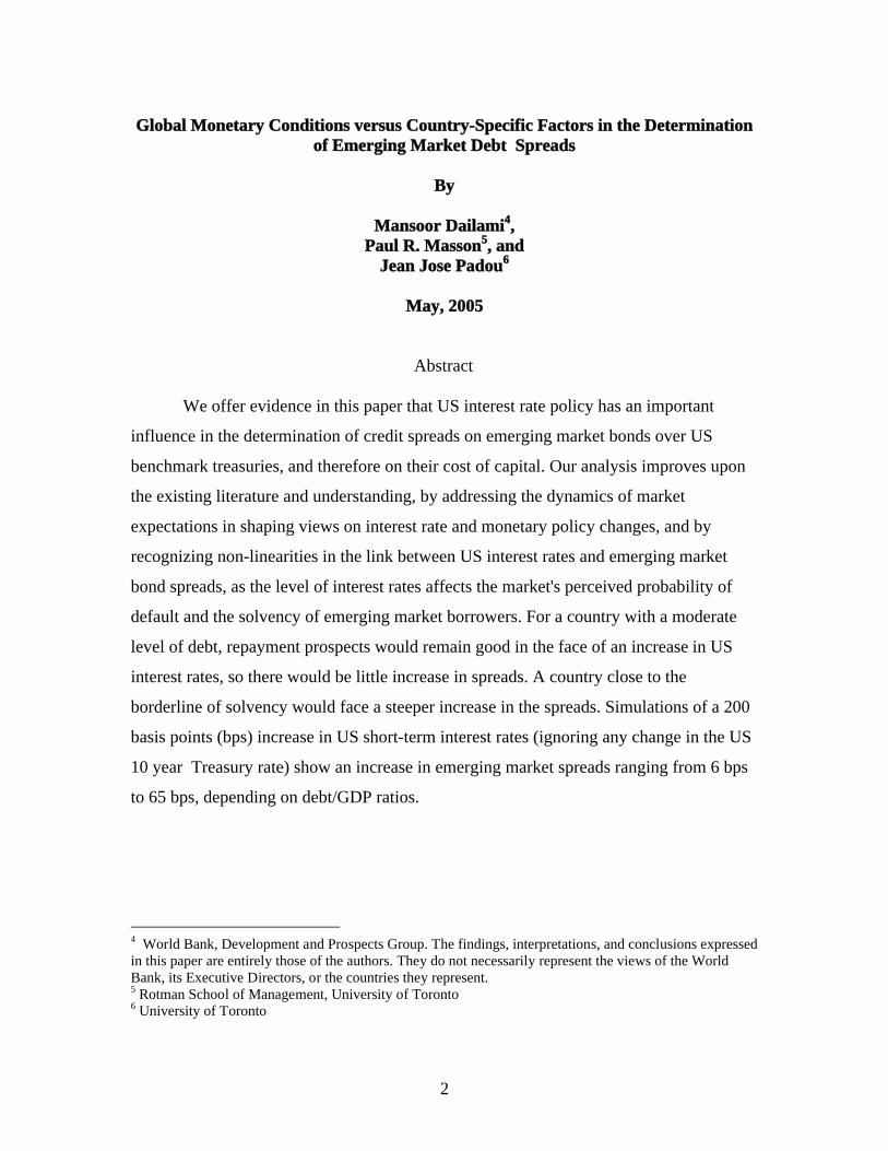
EM country is crucial to gauging the effect of US monetary tightening. As an illustration,
Figure 4 displays the impact a 200-basis-point increase in the U.S. T bill interest rate on
emerging market spreads (using the long-run estimates of Table 1, and assuming no
change in the long-term rate or corporate spreads): this translates into increases ranging
from 6 basis points (for countries with debt-to-GNI ratios below 40 percent) to 64 basis
points (for highly indebted countries with debt-to-GNI ratios above 90 percent).

24
Figure 4 Change in sovereign bond spreads from 200 basis point increase in U.S. interest rates for countries with different indebtedness
6
20
33
64
0
10
20
30
40
50
60
70
<40 40-60 61-80 >90
Debt/GNI (%)
Average change in spreads (bps)
Second, if the tightening of monetary conditions tips a country into a position of
default, then it might provoke a more widespread shift towards reduced risk appetite by
provoking a significant unwillingness of investors in EM debt to rollover existing debt or
extend new debt—what Calvo calls a “sudden stop.” This has occurred on at least half a
dozen occasions over the past two decades, and would correspond in our model to a shift
to a crisis equilibrium. While the causes of the crises are many, and there is no consensus
that US monetary policy was even an important contributing factor in each of them, the
debt crisis of August 1982 and Mexico’s devaluation of 1994 both followed a sharp
tightening of US monetary policy, and attacks on Asian currencies in 1997-98 and strain
on Argentina’s currency board in 2000-2002 came during a period of US dollar strength.
Subsequent abandonment of US dollar pegs (de facto or de jure) has no doubt left these
EM countries less vulnerable to currency crisis.
For a number of reasons it seems to us that the risk that US monetary tightening
might lead to dramatic increases in EM spreads and in global risk appetite is much lower

25
than in those past periods mentioned above. First, countries’ levels of indebtedness are
generally lower, as a ratio to GDP, than they were in those earlier periods, as countries
have learned the dangers of external borrowing, especially short term, and the level of
foreign exchange reserves is also considerably higher.18 However, countries are
differentially affected by the current high level of commodity prices, some benefiting
greatly through their commodity exports, while others may be mainly impacted by the
higher value of their oil imports.
Second, the fact that monetary tightening is largely anticipated (which was not the
case, for instance, in March 1994) is likely to lead to a less brutal adjustment of spreads
and to permit EM countries to take palliative measures in the meantime, including
lengthening maturities to lock in lower rates. For those countries that still limit the
fluctuations of their currencies against the US dollar, the fact that the dollar has
weakened against the euro and yen gives more room for maneuver.
Finally, there is evidence that investors are much more able to discriminate
among borrowers, and less likely to infer that problems in one country signal problems in
others.19 For instance, the default by Argentina in 2002—the largest default in history—
did not cause much disruption in world capital markets, nor did neighboring countries
suffer major increases in their spreads. Thus, should higher interest rates push a country
to the edge of default, the likelihood of generalized contagion seems much lower.
18 Though aggregate figures are very much influenced by China, India, Korea, and a few other Asian countries.19 Masson (2003) found that co-movement of EM spreads was lower in crises subsequent to the Asian crisis, indicating greater differentiation among countries.

26
References
Boss, M., and M. Scheicher, 2002, “The Determinants of Credit Spread Changes in the Euro Area,” BIS Papers No. 12, Bank of International Settlements, August 2002.
Camerer, Colin F. (1997), “Progress in Behavioral Game Theory,” Journal of Economic Perspectives, 11 (Fall): 167-88.
Colin-Dufresne, P., R. Goldstein, and S. Martin (2001), “ Determinants of Credit Spread Changes.” Journal of Finance 56, pp. 2,177-2,208.
Credit, 2004, Volume 5, Issue 06 (June), pp. 30-31, www.creditmag.com
Duffee, G R (1996), “Treasury Yields and Corporate Bond Credit Spreads: an Empirical Analysis”, Working Paper, Federal Reserve Board.
Duffee, G R (1998), “The Relationship between Treasury Yields and Corporate Bond Yield Spreads”, Journal of Finance, 53(6).
Eaton, Jonathan, and Mark Gersovitz (1981), “Debt with Potential Repudiation: Theoretical and Empirical Analysis,” Review of Economic Studies, 48: 289-309.
Elton,E., M. Gruber , D. Agrawal, and C. Mann, (2001), “ Explaining the Rate Spread on Corporate Bonds”, Journal of Finance 56, pp. 247-277.
Eichengreen, Barry, Andrew Rose, and Charles Wyplosz (1995), “Exchange Market Mayhem: The Antecedents and Aftermath of Speculative Attacks,” Economic Policy.
Eichengreen, Barry and Ashoka Mody, “Lending Booms, Reserves and the Sustainability of Short-term Debt: Inferences from the Pricing of Syndicated Bank Loans,” Journal of Development Economics, 63: 5-44.
Ferrucci, Gianluigi (2003), “Empirical Determinants of Emerging Market Countries’ Sovereign Bond Spreads,” Bank of England Working Paper 205.
Ferrucci, Gianluigi, Valerie Herzberg, Farouk Soussa, and Ashley Taylor (2004), “Understanding Capital Flows to Emerging Market Economies,” Financial Stability Review, London, June.
Jeanne, Olivier (1997), “Are Currency Crises Self-Fulfilling? A Test,” Journal of International Economics, 43(November): 263-86
Kaminsky, Graciela (1003), “Varieties of Currency Crisis”, NBER Working Paper 10193, December.

27
Kamin, Steven and Karsten von Kleist (1999), “The Evolution and Determinants of Emerging Market Credit Spreads in the 1990s”, International Finance Discussion Papers No. 653, Board of Governors of the Federal Reserve System (November).
Leake, Jeremy (2003), “Credit Spreads on Sterling Corporate Bonds and The Term Structure of UK Interest Rates”, Bank of England Working Paper 202, October.
Longstaff, F A and Schwartz, E. S. (1995), “A Simple Approach to Valuing Risky Fixed and Floating Rate Debt”, The Journal of Finance, 50: 789-820.
Masson, Paul (1999), “Contagion: Macroeconomic Models with Multiple Equilibria,” Journal of International Money and Finance (August).
_____ (2003), “Empirical Regularities in Emerging Market Spreads”, mimeo, Brookings Institution.
_____ (2001), “Multiple Equilibria, Contagion, and the Emerging Market Crises,” in R. Glick, R. Moreno, and M. Spiegel, eds., Financial Crises in Emerging Markets, (Cambridge, UK: Cambridge University Press).
Merton, R. (1974), “On the Pricing of Corporate Debt: The Risk Structure of Investment Rates”, Journal of Finance, 29, pp 449-470.
Min, Hong-Ghi, Duk-Hee Lee, Changi Nam, Myeong-Cheol Park, Sang-Ho Nam (2003), “Determinants of Emerging Market Bond Spreads: Cross-Country Evidence,” Global Finance Journal, 14: 271-86.
Morris, Stephen, and Hyun Song Shin (1998), “Unique Equilibrium in a Model of Self-Fulfilling Currency Attacks,” American Economic Review, 88(June): 587-97.
_____ (2002), “Rethinking Multiple Equilibria in Macroeconomic Modelling,” Macroeconomics Annual (Cambridge, MA: National Bureau of Economic Research).
Pesaran, M. Hashem, Yongcheol Shin, and Ron P. Smith (1999), “Pooled Mean Group Estimation of Dynamic Heterogeneous Panels,” Journal of the American Statistical Association 94 (June): 621-34
Uribe, Martin, and Vivian Z. Yue (2003), “Country Spreads and Emerging Countries: Who Drives Whom?” NBER Working Paper No. 10018, October.
28
Table 1. Long-Term Influences on Emerging Market Spreads, 1991M1-2004M620
Coefficient values (absolute t-ratios)explanatory variables full sample
(1)crisis periods
(2)non-crisis periods
(3)non-crisis periods
(4)(1) US variables
long-term interest rate -.0192(0.94) .2261(1.18) -.0143(.74) ..hi-low corporate spread .0739(9.08) .0601(0.57) .0794(10.0) .0796 (12.4)
(2) country specific variables
trade openness -.9260(24.2) -.0640(.08) -.918(23.6) -.913 (23.9)debt/gni .0093(7.75) .0200(2.82) .0087(7.77) .0089 (8.09)
reserves/debt -.0212(15.9) -.0622(8.01) -.0194(16.0) -.0191 (16.0)short-term/total debt -.0291(19.8) -.1055(4.37) -.0283(20.2) -.0280 (20.1)
(3) interaction variablesUS Tbill rate times country’s debt/gni
.00066(3.21) .0011(0.69) .00084(4.31) .00081 (4.35)
contagion dummy .0115(1.20) -.2123(2.56) .0186(1.97) ..constant 6.944(37.5) 7.213(6.36) 6.779(38.9) 6.707 (89.1)
(4) statisticsno. of obs. 1551 54 1497 1497
R2 .5785 .8243 .5976 .5960p-value for zero coeffs .0000 .0000 .0000 .0000
20 Period of estimation depends on the country’s data availability. Static regression of the log of spreads on the explanatory variables listed above, with all coefficients constrained to be the same for all countries.

29
Table 2. Forecasting Equations for First Differences in US Interest Rates1992M5-2004M6
Coefficient values (absolute t-ratios)Explanatory variables: changes in logs of:
US Tbills 10-year Treasuries Corporate Hi-Lo Spread
Producer PriceLag 1 2.400 (1.29) 4.438 (1.68) -4.359 (.76) Lag 2 2.308 (1.23) -2.677 (1.01) 4.176 (.73)Lag 3 -2.716 (1.48) -4.973 (1.90) .356 (.06)
Retail SalesLag 1 2.751 (1.95) 6.266 (3.13) -9.099 (1.62)Lag 2 5.643 (3.84) 6.826 (3.27) 1.745 (.39)Lag 3 2.791 (1.99) 3.612 (1.81) -2.408 (.56)
Capacity Utilization
Lag 1 10.124 (3.54) 5.524 (1.36) 4.291 (.49)Lag 2 3.604 (1.24) .425 (.10) -3.769 (.42)Lag 3 7.128 (2.38) .707 (.16) -11.098 (1.21)
M2Lag 1 -3.081 (1.37) 8.563 (2.67) -12.034 (1.74)Lag 2 -2.082 (.96) -.547 (.18) -1.761 (.26)Lag 3 -3.601 (1.57) 1.201 (.37) -3.812 (.54)
Constant -.0324 -.1303 .1163No. of obs. 146 146 146R2 .3418 .1796 .068p-value .0000 .0000 .0000

30
Table 3. Dynamic Error Correction Models for Changes in Log Spreads: Fixed Effects, Non-crisis periods, 1991M1-2004M6
Coefficient values21 (absolute t-ratios)explanatory variables Actual US interest
rate changes only(1)
Actual and forecast US interest rate
changes (2)
Parsimonious model
(3)(1) lagged residual from Column 4 of Table 1
-.1040 (9.33) -.1037 (9.12) -.1035 (9.13)
(2) changes in US Interest Rate Variables
US T Bills .0338 (1.66) .00092 (.04) ..10 year Treasuries .0653 (3.41) .0674 (3.46) .0671 (3.66)
US hi-low corporate spread
.1274 (16.9) .1280 (16.6) .1288 (17.0)
Forecast US T Bills .. .0660 (1.36) .0735 (1.96)Forecast 10yr Treasuries .. .0114 (.21) ..
Forecast US hi-low spread
.. .1619 (4.26) .1513 (4.92)
(3) changes in country specific variables
trade openness .1016 (.96) .0982 (.93) ..debt/gni .00888 (2.49) .00894 (2.49) .00974 (2.74)
reserves/debt -.0219 (3.35) -.0220 (3.35) -.0237 (3.63)short-term/total debt -.0281 (3.55) -.0302 (3.77) -.0304 (3.81)
(4) contagion dummy .00288 (.97) .00444 (1.47) ..(5) statistics
no. of obs. 1471 1441 1443R2 Within .2218
Between .3108Overall .1960
Within .2369Between .3161Overall .2119
Within .2368Between .3080Overall .2122
p-value for zero coefficients
.0000 .0000 .0000
p-value for test all u(i)=0 .0009 .0033 .0038
21 Separate country intercepts are not reported.

31
Table 4. Pooled-Mean-Group Dynamic Error Correction Models for Changes in Log Spreads: Fixed Effects, Non-crisis periods, 1991M1-2004M6
Coefficient values22 (absolute t-ratios)Explanatory variables Full model Parsimonious
model(1) Long-run coefficients
10-yr Treasury rate -.2301 (4.29) -.2058 (4.41)US hi-low corporate
spread.00585 (.29) .00753 (.43)
US Tbill rate times country’s debt/gni
.000775 (1.80) .000562 (1.48)
trade openness -.4676 (1.84) -.5352 (2.27)debt/gni .00471 (1.21) .00734 (2.08)
reserves/debt -.0221 (3.40) -.0225 (3.83)short-term/total debt -.00628 (.77) -.00116 (.16)
(2) coefficient on lagged EM spread, by country:
Argentina -.0720 (2.08) -.0577 (2.03)Brazil -.1312 (3.28) -.1301 (3.39)
Bulgaria -.1372 (3.00) -.1362 (3.04)Colombia -.3232 (1.92) -.2851 (1.87)Ecuador -.1286 (3.28) -.1315 (3.41)Mexico -.1699 (2.96) -.1823 (3.10)
Morocco -.1601 (3.99) -.1547 (4.14)Nigeria -.1393 (3.93) -.1188 (3.99)Panama -.4963 (3.50) -.5228 (3.67)
Peru -.4452 (3.81) -.1420 (5.11)Philippines -.1405 (2.50) -.1461 (2.91)
Poland -.1545 (2.64) -.1339 (2.70)Russia -.1205 (2.74) -.1254 (2.97)
South Africa -.0191 (.39) -.0157 (.37)Turkey -.3084 (1.47) -.3139 (1.98)Ukraine -.3742 (1.76) -.3420 (2.04)
Venezuela -.1321 (3.20) -.1345 (3.39)(3) statistics
no. of obs. 1443 1443R2 .3294 .3194
Adjusted R2 .2458 .2703p-value for zero
coefficients.0000 .0000
22 Coefficients on the explanatory variables in first-differences and separate constant terms, which are allowed to differ across countries, are not reported.

32
Appendix: List of Variables
variable name definition source
EM spread Emerging Market Bond Index JP Morgandebt/gni total debt /Gross National Income GDF, World Bank
short-term debt/total debt GDF, World Banktradeop (imports+exports of G&S)/GDP IFS, IMF
reserves/debt for. exchange reserves/total debt GDF, World BankUS long-term interest rate government 10-year bond yield US BEA
US Tbill rate secondary market yield, 3-mo. treas. bill US BEAUS hi-low corp. spread Moody’s Baa-Aaa corp. bond yield US BEA
crisis dummy =1 if country in crisis, otherwise 0 Kaminsky (2003)contagion dummy =n if n other countries are in crisis based on Kaminsky (2003)
US producer price index US BEAUS capacity utilization Industrial sector US BEA
US retail sales All sectors US BEAUS M2 Federal Res. Board