Federal Reserve Bank of Minneapolis Research Department Staff Report 489 Revised: June 2014 (First version: August 2013) Global Imbalances and Structural Change in the United States* Timothy J. Kehoe University of Minnesota, Federal Reserve Bank of Minneapolis, and National Bureau of Economic Research Kim J. Ruhl Stern School of Business, New York University Joseph B. Steinberg University of Toronto

ABSTRACT___________________________________________________________________

Since the early 1990s, as the United States has borrowed from the rest of the world, employment in the U.S. goods-producing sector has fallen. We construct a dynamic general equilibrium model with two mechanisms that could generate declining goods-sector employment: foreign lending and differential productivity growth across sectors. We find that 18 percent of the decline in goods-sector employment from 1992 to 2012 follows from U.S. trade deficits. Most of the decline in employment in the goods sector can be accounted for by differences in productivity growth across sectors. As the United States repays its debt, its trade balance will reverse, but goods-sector employment will continue to fall.

Keywords: Global imbalances; Real exchange rate; Structural change JEL classification: E13, F34, O41 _____________________________________________________________________________________________

*We thank David Backus, David Strauss, Frank Warnock, Kei-Mu Yi, and Vivian Yue for helpful discussions. Kehoe and Ruhl gratefully acknowledge the support of the National Science Foundation under grant SES-0962993. We are grateful to Jack Rossbach for extraordinary research assistance. The data used here are available at http://www.econ.umn.edu/~tkehoe. The views expressed herein are those of the authors and not necessarily those of the Federal Reserve Bank of Minneapolis or the Federal Reserve System.

1

1. Introduction

Between 1992 and 2012, households and the government in the United States borrowed heavily

from the rest of the world, and the U.S. net international investment position deteriorated by $4

trillion. A commonly held view in policy circles, expressed, for example, by Bivens (2006) and

Scott, Jorgensen, and Hall (2013), is that the U.S. trade deficits generated by this borrowing have

played an important role in the decline of employment in the U.S. goods-producing sector and

that an end to these deficits will reverse a large part of this trend.

We use a dynamic general equilibrium model of the United States and the rest of the

world to address the questions: To what extent are trade deficits responsible for the loss of U.S.

goods-sector employment? Will employment return to goods-producing sectors when U.S.

borrowing ends and trade deficits become trade surpluses?

Our framework combines an open economy model of foreign lending and a model of

structural change — the secular shift of employment from goods-producing industries to

services-producing industries — that has been typically studied in a closed economy. Structural

change in our model is driven by differential productivity growth across sectors as in Ngai and

Pissarides (2007). Faster productivity growth in the goods-producing sector, combined with a

low elasticity of substitution between goods and services, generates the structural change in the

composition of employment. We use this model to quantitatively assess the relative

contributions of asymmetric labor productivity growth and the saving glut to the decline in

goods-sector employment in the United States.

Our calibrated model of structural change and trade imbalances accounts for 78 percent

of the decline in goods sector employment from 1992 to 2012. (Notably, we do not model the

U.S. recession in 2007–2009 except through its impact on the trade balance.) In the model, U.S.

trade deficits accounted for 17.7 percent of the decline in the goods-producing sector’s

employment between 1992 and 2012, with most of the remainder attributed to faster productivity

growth in the goods sector relative to other sectors. This implies that eliminating the trade

deficit will not generate a significant increase in goods-sector employment. We find that, if the

trade deficit gradually changes to a surplus, U.S. borrowing in the 1990s and 2000s has been

welfare improving. If the trade balance reverses quickly and unexpectedly — a sudden stop, like

that in Mexico in 1995–1996 — then welfare would be greater if the United States had not

borrowed.

2

It is easy to see why some view trade deficits as detrimental to goods-sector employment.

Figure 1 shows that the share of employment in the goods sector — agriculture, mining, and

manufacturing — has fallen dramatically as the trade deficit has grown. The intuition for this

idea is simple: Imported goods are substitutes for domestically produced goods. As the United

States trades bonds for foreign goods, labor shifts away from domestically produced goods and is

reallocated to producing services and construction, which are less substitutable for foreign goods.

When the debt has to be repaid, labor will flow back into the goods sector to produce the extra

goods needed to repay the debt. The importance of this channel for U.S. goods-sector

employment is the quantitative question at the center of our study.

In constructing the model, we need to specify the driving force behind U.S. borrowing.

A common explanation is that foreign demand for saving increased, making foreigners more

willing to trade their goods for U.S. bonds. Bernanke (2005) coined the term global saving glut

to refer to this idea, and we adopt Bernanke’s global-saving-glut hypothesis. Several

explanations have been proposed for the increased demand for saving in the rest of the world,

such as a lack of financial development in the rest of the world (Caballero, Farhi, and

Gourinchas, 2008; Mendoza, Quadrini, and Ríos-Rull, 2009), differences in business cycle or

structural growth properties (Backus et al., 2006; Perri and Fogli, 2010; Jin 2012), and

demographic differences (Du and Wei, 2013). We do not take a stand on which of these

explanations, if any, are correct. Instead, we take the saving glut as given and calibrate a process

for the preferences of households in the rest of the world over current versus future consumption

so that our model matches exactly the path of the U.S. trade balance between 1992 and 2012.

We include four features in the model that make it well suited to address these issues.

First, we model an economy with three sectors: goods, services, and construction. Goods and

services can be traded, which allows us to capture the fact that the United States consistently

runs a substantial trade surplus in services. International macroeconomic models usually treat

goods as the only tradable sector and lump all other sectors into a single nontradable sector. This

assumption is at odds with the data: Services are a large component of U.S. exports.

Construction is the only nontradable sector and is used almost entirely to produce investment

goods, which means that construction is more sensitive than the other sectors to the effects of

capital flows and economic fluctuations in general. Second, we build a detailed input-output

structure into the production side of the model. This allows us to model the elasticity of

3

substitution between goods, services, and construction in production as well as consumption.

Third, we allow the elasticity of substitution between foreign and domestic inputs to differ across

sectors. Our calibration assigns a higher elasticity of substitution between domestic and foreign

inputs in the goods sector to match the fact that the goods trade balance is more volatile than the

services trade balance, as seen in figure 6.

Fourth, and perhaps most important, we allow labor productivity to grow at different

rates across sectors, matching the fact that labor productivity in the goods sector grew at a faster

pace than in other sectors over the past two decades, as seen in figure 2 The structural change

literature emphasizes asymmetric productivity growth as an important driver of the long-run

reallocation of labor across sectors. Recent studies embed this mechanism, originally due to

Baumol (1967), into closed-economy models that are consistent with aggregate balanced growth

(Ngai and Pissarides, 2007; Buera and Kaboski, 2009). We take a similar approach in an open

economy model. Several other recent papers study structural change in open economies

(Echevarria, 1995; Matsuyama, 1992, 2009; Sposi, 2012; Uy, Yi, and Zhang, 2013). With the

exception of Sposi (2012), these studies use models of balanced trade, abstracting from

international capital flows. Allowing for unbalanced trade, we can assess the relative

contributions of traditional structural change forces and the saving glut to the dynamics of the

U.S. economy.

Buera and Kaboski (2012) identify three possible sources of structural change:

differential sectoral productivity growth and a low elasticity of substitution between sectors

(Ngai and Pissarides, 2007); nonhomothetic preferences (Kongsamut, Rebelo, and Xie, 2001);

and capital deepening and sector-specific capital shares (Acemoglu and Guerrieri, 2008). As

argued by Buera and Kaboski (2012), nonhomothetic preferences are most relevant at low levels

of income and are thus unlikely to be important for the United States. We allow for sector-

specific capital shares in our model, but they do not play a quantitatively important role in our

results.

We calibrate our model so that it matches exactly the national accounts and input-output

table for the United States in 1992 and the U.S. trade balance during 1992–2012. As figures 5–7

show, our calibrated model endogenously generates outcomes that match several key facts about

the U.S. economy during this period: We match the magnitude of the real exchange rate

4

appreciation and subsequent depreciation, the dynamics of the disaggregated goods and services

trade balances, and the changes in sectoral employment shares.

We use the model to conduct two kinds of exercises: historical counterfactuals and

predictions about the future. In our counterfactual scenario, we turn off the saving glut, which

allows us to answer questions about the path the U.S. economy would have taken had the saving

glut never occurred. In our model without a saving glut, the goods sector’s employment share

falls from 19.7 percent in 1992 to 15.1 percent in 2012 compared with 14.1 percent in the model

with the saving glut and to 12.5 percent in the data. Looking to the future, our benchmark model

predicts that the goods sector’s employment share will continue to decline in the long run, and

that the trade balance reversal required to repay the debt the United States incurred during the

saving glut will have little impact on goods-sector employment. The goods sector’s employment

share is 13.1 percent in 2024 in our benchmark, versus 12.6 percent in the counterfactual

scenario in which the saving glut never occurs.

Our model allows us to ask: To what extent has the saving glut been good for U.S.

households? We construct a measure of the real income of U.S. households in 1992, and

compare the welfare of U.S. households in the baseline model to a counterfactual in which the

saving glut did not occur. The saving glut itself improves welfare: The lifetime real income of

U.S. households in 1992 would have been almost $700 billion lower (about 11 percent of 1992

GDP) if the saving glut had not happened. In our baseline model, we assume that the transition

from a trade deficit to a surplus will happen gradually.

In an extension, we consider the effects of a sharp reversal of the trade balance — a

sudden stop — as suggested in Obstfeld and Rogoff (2005, 2007). Our results indicate that a

sudden stop in the United States in 2015–2016 would look similar to historical episodes in

emerging economies: a large real exchange rate depreciation, a substantial productivity-driven

output contraction, and a sharp reallocation of factors across sectors (Calvo, Izquierdo, and

Mejía, 2004; Calvo and Talvi, 2005; Kehoe and Ruhl, 2009). As in sudden stops of the past,

these effects would be short-lived; several years after the sudden stop ends, the U.S. economy

would be on almost the same path on which it would have been if the sudden stop had never

happened. Any temporary reallocation of labor to the goods-producing sector during the sudden

stop would be quickly reversed and have no long-term effect.

5

In the sensitivity analysis of our model, we find that our main results are robust to a

range of modeling choices, such as altering our assumptions about the path of government

spending and abandoning perfect foresight in favor of a stochastic model with rational

expectations. The input-output production structure and the tradability of services, however,

play important quantitative roles in our model’s predictions for goods-sector employment.

Removing the input-output structure raises the elasticity of substitution between goods and

services in gross output, which causes our model to capture a significantly smaller fraction of the

decline in goods-sector employment we observe in the data during 1992–2012. This change also

leads our model to overstate the role of the saving glut in reducing goods-sector employment

during this period; making services nontradable has a similar effect.

To justify our assumption that the U.S. trade deficit has been driven by the rest of the

world’s demand for saving rather than domestic factors, we study a version of our model in

which we alter the preferences of U.S. households — rather than those in the rest of the world —

to match the U.S. trade balance. This domestic-saving-drought experiment does not significantly

affect our main results about goods-sector employment, but it leads to predictions for investment

and construction employment that are sharply at odds with the data: The foreign-saving-glut

hypothesis fits the data better.

2. The U.S. economy, 1992–2012

This section presents our approach to analyzing U.S. data over the past two decades. We view

the massive foreign borrowing and the differentials in productivity growth across sectors as

exogenous driving forces that we take as inputs into the model. Below, we present three key

facts about U.S. data that we view as tests for our model. It is our model’s ability to replicate

these three facts in response to the exogenous driving forces that gives us confidence in using the

model to make predictions about the future of the U.S. economy.

Exogenous driving force 1: Foreign borrowing increased, then decreased

Figure 3 illustrates just how much borrowing households and the government in the United

States have done. The current account balance measures the exact magnitude of capital flows

into the United States, but we see that the trade balance tracks the current account balance almost

exactly. Since our model is not designed to accurately capture the difference between these two

6

series, and the trade balance has an exact model analogue, we use the trade deficit as our

measure of U.S. borrowing. Figure 3 shows that between 1992 and 2006, the trade deficit grew

steadily, reaching 5.8 percent of GDP, after which it began to shrink. In 2012, the trade deficit

remained at 3.6 percent of GDP. We view the path of the trade balance as what defines the

saving glut in our model. Our hypothesis is that the U.S. economy is currently in the process of

emerging from the saving glut.

Capital flows are important to our analysis in two ways. First and foremost, the

imbalanced flow of goods into the United States directly affects the need to produce goods

domestically and, thus, the labor needed in that sector. The trade balance is the most appropriate

measure of this force. Second, the accumulated debt eventually needs to be repaid, which could

affect the future employment needed to produce goods in the United States. In the model,

accumulated trade balances are the measure of this accumulated debt, which differs from the

U.S. net foreign asset position by any revaluation effects. These revaluation effects have, at

times, played a significant role in the value of the U.S. net foreign asset position (Lane and

Milesi-Ferretti, 2008; Gourinchas and Rey, 2007). To the extent that revaluation has been in the

favor of the United States, the smaller future debt burden would decrease the need to reallocate

labor back into the goods-producing sectors.

Exogenous driving force 2: Labor productivity grew fastest in the goods sector

During 1992–2012, labor productivity in the goods sector increased by an average of 4.2 percent

per year, while it increased by only 1.3 percent per year in the services sector and fell by 1.2

percent per year in construction. What is essential in our model is the differential between

productivity growth in the goods sector and that in the services sector. As the data in figure 2

show, this differential has been close to constant since 1980, with average productivity growth of

4.1 percent per year in goods during 1980–2012, compared with 1.3 percent in services. Except

for the productivity slowdown of the 1970s, the differential has been persistent since 1960. Our

hypothesis is that this productivity differential persists until at least 2030.

Fact 1: The real exchange rate appreciated, then depreciated

Figure 3 presents the first key fact that we ask our model to replicate. The figure shows that the

U.S. real exchange rate was volatile and tracked the trade balance closely during 1992–2012.

7

We construct our measure of the U.S. real exchange rate by taking a weighted average of

bilateral real exchange rates with the United States’ 20 largest trading partners, with weights

given by these countries’ shares of U.S. imports in 1992. (Other weighting schemes do not

significantly affect our results.) This approach forms the basis of our concept of the rest of the

world in our model. The real exchange rate appreciated by 27.9 ( 100 (100 / 78.2 1) ) percent

between 1992 and 2002, after which it depreciated by 22.1 percent between 2002 and 2012. The

intuition for why the real exchange rate and trade balance should move closely is

straightforward: As foreign goods and services become cheaper, U.S. households buy more of

them. Notice, however, that the timing is off: The maximum appreciation of the real exchange

rate occurred in 2002, whereas the largest trade deficit occurred in 2006.

Fact 2: The goods sector drove aggregate trade balance dynamics

Figure 6 presents our second key fact. Here we disaggregate the trade balance, plotting the trade

balances for goods and services separately. We see that the goods trade balance generates most

of the fluctuations in the aggregate trade balance, whereas the services trade balance fluctuates in

a band between 0.5 and 1.2 percent of GDP. That the United States has consistently run a trade

surplus in services motivates one of the key features of our modeling framework. Standard

modeling conventions in international macroeconomics lump services together with construction

into a nontradable sector, treating goods as the only sector that produces output that can be

traded internationally. By contrast, we allow both goods and services to be traded in our model,

and we calibrate home bias parameters — the share parameters in the Armington aggregators —

for each sector separately to capture the fact that the United States consistently runs a surplus in

services and a deficit in goods.

Fact 3: Employment in goods declined steadily; construction employment rose, then fell

Figure 7 presents our third fact: Between 1992 and 2012, the fraction of total labor

compensation paid to the goods sector fell from 19.7 percent to 12.5 percent. The fraction of

total labor compensation is our preferred measure of the goods sector’s employment share

because it maps directly into our model, where we measure labor inputs in terms of effective

hours worked, rather than raw hours worked. As figure 1 shows, this measure moves closely

with more common measures like the share of employees in the goods sector; the same is true for

8

the construction sector. The construction sector’s share of labor compensation rose from 4.4

percent in 1992 to 5.7 percent in 2006, as construction boomed prior to the financial crisis in

2008–2009. Employment in construction then started to fall, and by 2012 the construction

sector’s share of labor compensation was again 4.4 percent.

3. Model

We model an economy with two countries, the United States and the rest of the world (RW). We

use the superscripts us and rw to denote prices, quantities, and parameters in the United States

and the rest of the world. The length of a period is one year. Each country has a representative

household that works, consumes, and saves to maximize utility subject to a sequence of budget

constraints. The model begins in 1992, is subject to transitory — though decades long —

changes in sectoral productivity growth rates and the rest of the world’s willingness to lend, and

eventually settles onto a long-run balanced growth path.

Each country produces commodities that serve both intermediate and final uses. We

model the U.S. production structure in detail, using an input-output structure that we calibrate to

the U.S. input-output matrix. We model production in the rest of the world in a simpler fashion,

abstracting from investment and domestic input-output linkages. We model the U.S. government

in a reduced-form fashion as well — the government’s spending and debt are specified

exogenously, and the government levies lump-sum taxes on U.S. households to ensure that its

budget constraints are satisfied.

Financial assets

The U.S. government, households in the United States, and households in the rest of the world

have access to a one-period, internationally traded bond, tb , that is denominated in units of the

U.S. consumer price index (CPI). U.S. households can also save by investing in the U.S. capital

stock, but will be indifferent between holding capital and bonds because they both pay the same

return in equilibrium. We model a single bond, but the equilibrium of our baseline model is

equivalent to one in which both governments and households issue debt. The deterministic

nature of the model gives rise to Ricardian equivalence (except at the onset of the savings glut),

so the split between public and private debt is essentially irrelevant. In section 6 we present a

9

stochastic version of the model in which public and private debt are distinct, but we find this

change to be quantitatively insignificant.

Production

The United States produces four commodities: goods sgtuy , services s

stuy , construction s

ctuy , and

investment situy . The rest of the world produces its own goods w

gtry and services w

stry . Prices are

denoted analogously. All commodities are sold in perfectly competitive markets. Each U.S.

commodity , ,j c g s is produced using capital sjtuk and labor s

jtu , along with intermediate inputs

of U.S. goods sgjtuz , U.S. services s

sjtuz , U.S. construction s

cjtuz , and imports us

jtm purchased from the

same sector j in the rest of the world:

(1) 1

1

min , , , (1 )

j j

j jj

us us usgjt sjt cjtus us us us us

jt j j j jt jt jt j jtus us usgj sj

us us us u

j

s

c

z zy

a

zM m

a aA k

.

This nested production function embeds a Leontief input-output structure in an Armington

aggregator. The parameters of the production functions are: usjM and us

jA , the constant scaling

factors used to facilitate calibration; usj , which governs the share of imports in production; j ,

which governs the elasticity of substitution between domestic and imported inputs; , ,us us usgj sj cjaa a ,

which govern the shares of goods, services, and construction in gross output; usjt , the sector-

specific labor productivity; and j , capital’s share of value added.

Our assumption of zero substitutability between intermediate inputs is standard in the

input-output literature, consistent with empirical findings that direct requirement coefficients

vary little over time (Sevaldson, 1970; Miller and Blair, 2009). This assumption implies that the

elasticity of substitution between goods and services in both intermediate and final uses is lower

than the same elasticity in final uses alone. In section 6, we show that this assumption plays an

important role in our model’s ability to capture the reallocation of labor across sectors that we

observe in the data.

We allow the Armington elasticities 1 / (1 )j to differ across sectors to capture the fact

that the goods trade balance is more volatile than the services trade balance (see figure 6). We

10

also allow labor productivity usjt to grow at different rates across sectors to capture the fact that

productivity in the goods sector has grown faster than in other sectors. This differential

productivity growth is the driving force behind the structural change mechanism in the model.

U.S. producers in all three sectors , ,j g s c choose inputs of intermediates and factors to

minimize costs, which implies standard marginal product pricing conditions for capital and labor.

The U.S. investment good is produced using inputs usgitz , us

sitz , and uscitz of goods, services,

and construction according to

(2) g s cus usit git sit ci

us usty z z zG

, 1g s c .

This specification is consistent with evidence reported by Bems (2008) that expenditure shares

on investment inputs are approximately constant over time across a range of countries.

We model the rest of the world’s production structure in less detail, abstracting from

investment and input-output linkages. Goods and services in the rest of the world are produced

using labor rwjt and imported intermediate inputs rw

jtm from the same sector j in the United

States. The production functions are simpler nested Armington aggregators of the form

(3) 1

(1 )j j jrw rw rw rw rw rw rw

jt j j jt jt j jtM my .

Households

Each country is populated by a continuum of identical households. We draw a distinction

between the total and working-age populations so that our model can capture the impact of

demographic changes on households’ incentives to borrow and save. We denote the total U.S.

population by ustn and the working-age population by us

t . We evaluate consumption per capita

on an adult-equivalent basis, defining the U.S. adult-equivalent population as

( ) / 2us us us ust t t tnn . The rest of the world’s demographic variables are defined

analogously.

We normalize the amount of time available for work and leisure by a U.S. working-age

person to one and denote total U.S. labor supply by ust . U.S. households choose labor supply,

11

consumption of composite goods and services ushgtc and ush

stc , investment usti , and bond holdings

ushtb to maximize utility

(4) (1 )

1

0

(1 )ush ush us us

ush ush stus u

gtt t t

t t ts us

t

c c

n n

subject to the budget constraints

(5) 1 ( , ) (1 )us us usgt gt st st it t tus ush us ush us us ush us us ush

t t t gt st t k ktus us us u

t tsp p w p p p rc c p i q b b k T ,

the law of motion for capital

(6) 1 (1 )us us ust t tkk i ,

appropriate non-negativity constraints, initial conditions for the capital stock and bond holdings

0usk and 0

ushb , and a constraint on bond holdings that rules out Ponzi schemes but does not

otherwise bind in equilibrium. We use the superscript ush for U.S. households’ consumption

and bond holdings to distinguish them from those of the U.S. government, for which we use the

superscript usg . Households pay constant proportional taxes usk on capital income and a lump-

sum tax or transfer ustT . We use the capital income tax to obtain a sensible calibration for the

initial capital stock and depreciation rate. We also allow the tax rate on capital income in 1993

to differ from the constant rate in order to match the level of investment in 1992.

Bonds are denominated in units of the U.S. CPI, defined as

(7) 1992 1992

1992 1992 1992 1992

( , )us ush us ugt g st

sh

us ush

sus us usgt st

g g s sus ush

p c c

c

p

cp p p

P P

.

We model discount bonds, so the price tq represents the price in period t of one unit of the U.S.

CPI basket in period 1t . The real interest rate in units of the U.S. CPI is given by

(8) 1 ( , /1 )us us ust gt st tp p p qr .

During the sudden stop episode that can occur in 2015, bond holdings are fixed and the internal

real interest rate is determined endogenously in each country separately. The market clearing

condition for bonds is

12

(9)(9) 0 usg ush rwt t tb b b .

The rest of the world’s households solve a simpler problem. We abstract from

investment dynamics in the rest of the world, so the only way the rest of the world’s households

can save is by buying U.S. bonds. We can easily allow for rest-of-the-world bonds as well

without changing the equilibrium of the model. Labor supply is endogenous and the rest of the

world’s households have a utility function similar to that of U.S. households:

(10) (1 )

1

0

(1 )rw rw rw rw

rw rw strw r

gtt rw t tt w r

t t tw

t

c c

n n

.

The only differences from the U.S. households’ utility function are the share parameter rw and

the utility weight rwt . The latter is an intertemporal demand shifter, which we calibrate to

match the U.S. trade balance during 1992–2012. During this period rwt falls, reflecting a

reduction in utility gained from consumption at t compared with future consumption. This is the

driving force behind the saving glut. The rest of the world’s representative household chooses

labor supply rwt , consumption of goods and services rw

gtc and rwstc , and bond holdings rw

tb to

maximize utility subject to the budget constraints,

(11) 1 ( , )rw rw rw rw r rww rrw us us usgt gt st st t t t t gt t

ws tp c c q b w bp p p p ,

and non-negativity and no-Ponzi constraints similar to those that U.S. households face. The rest

of the world’s CPI is defined analogously to the U.S. CPI in (7) . The real exchange rate is

(12) ( , ) / ( , )rw rw rw us us ust gt st gt strer p p p p p p .

U.S. government

The government in the United States levies taxes and sells bonds to finance exogenously

required expenditures on consumption of goods and services. The budget constraint is

(13) 1 ( , )us us us ususg usg usg us us us usggt gt st st t t k kt t t gt st

s ust

up c Kc p q b r T p p p b .

We specify exogenous time paths for total government consumption expenditures and debt as

fractions of GDP, using historical data for 1992–2012 and Congressional Budget Office (CBO)

13

projections for the future. We use t and t to denote these time series. We allow the lump-

sum tax ustT to vary as necessary to ensure that the government’s budget constraint is satisfied.

To allocate its total expenditure between goods and services, in each period, the

government chooses usggtc and usg

stc to maximize

(14) usg usgusg usggt stc c

subject to the constraint that the government makes its required total expenditures. We assume

that government spending does not enter the household’s utility function (or equivalently, enters

in a separable fashion), nor does it enter any of the production functions.

Because of the lump sum tax, our model exhibits near-Ricardian equivalence. That is,

the timing of taxes and government borrowing is almost irrelevant. Ricardian equivalence

breaks down only when we introduce unexpected events — the saving glut and the sudden stop.

Unanticipated changes in the time path of government debt that accompany these events do

affect the model’s equilibrium dynamics, particularly in the short run.

Equilibrium

An equilibrium in our model, for a given sequence of time-series parameters 0{ , , }rwt t t t

and

initial conditions 0 0 0( ), ,ush usg usb b k , consists of a sequence of all model variables such that

households in the United States and the rest of the world maximize their utilities subject to their

constraint sets, prices and quantities satisfy marginal product pricing conditions for all

commodities, prices and quantities are such that all production activities earn zero profits, all

commodity, factor, and bond market clearing conditions are satisfied, and the U.S. government

solves its consumption-spending allocation problem in each period. When we solve the model

numerically, we require that equilibria converge to balanced growth paths after 100 years. There

are an infinite number of possible balanced growth paths — indexed by the sum of public and

private U.S. debt — but our model’s equilibrium is unique, because the initial conditions

determine onto which balance growth path the economy settles.

4. Calibration

We calibrate the model’s parameters and initial conditions so that the equilibrium replicates the

U.S. input-output matrix and national accounts for 1992. We do this for a model in which the

14

agents do not foresee the savings glut. We view this as the most natural way to think about the

agents’ expectations in the early 1990s: We do not think that U.S. households in 1992 foresaw

the kind of borrowing the United States would do over the subsequent two decades. Table 2 lists

our calibrated parameter values. More details are provided in the online appendix at

http://www.econ.umn.edu/~tkehoe.

U.S. production parameters

We choose units so that U.S. GDP is equal to 100 and all prices are equal to 1 in 1992. We

compute the parameters in the Leontief portion of the U.S. production functions in (1) directly

from the input-output matrix shown in table 1. For example, to compute usgca , the amount of

goods needed to produce one unit of gross output in the construction sector, we divide the value

in the goods row and construction column (3.7) by gross output in construction (10.7). We use a

similar procedure to calculate factor shares in value added for each sector. For the Armington

aggregators in (1), we first specify values for the elasticities of substitution between domestic

and imported inputs. There is some debate over this elasticity because business cycle models

tend to imply a low elasticity, whereas analysis of trade policy changes often suggests a much

higher elasticity; see Ruhl (2008) for a detailed discussion. Because the services trade balance is

less volatile than the goods trade balance, we choose a lower elasticity of substitution between

domestic and foreign inputs in the services sector. We set the elasticity in goods 1 / (1 )g to 3

and that in services 1/ (1 )s to 1. We then use equilibrium conditions (marginal product

pricing and zero profits) to calibrate usj from the input-output matrix. The scale factors us

jM

are set so that equilibrium outputs match their respective entries in the input-output table. We

use a similar procedure to calibrate the production function for investment.

Household and government parameters

We set the elasticity of intertemporal substitution 1 / (1 ) to 0.5. We set the long-run interest

rate to 3 percent (U.S. Congress, Congressional Budget Office, 2012) and the discount factor

so that this interest rate is consistent with balanced growth. We set the elasticity of substitution

between goods and services in consumption, 1 / (1 ) , to 0.5, as in Stockman and Tesar (1995).

We calibrate the parameters ush and of the households’ preferences using private

15

consumption data from the input-output table and data on hours worked. A similar procedure

yields the government’s share parameter usg .

U.S. initial conditions

To calculate the initial capital stock, we set the 1992 real interest rate to 4 percent. The real

interest rate in 1992 is not an equilibrium object in our model; it would have been determined in

1991, but 1992 is our initial model year. The real interest rate on 10-year U.S. Treasury bonds

was approximately 4 percent in 1992. Given a tax rate on capital income usk , we can compute

our initial capital stock using data on depreciation from the 1992 national income accounts and

data on payments to capital in the input-output table. We choose 0.4usk , which implies a

depreciation rate of 6.6 percent per year, well within the standard range of annual depreciation

rates found in the literature. Our results are not sensitive to alternative approaches to calibrating

the initial capital stock. U.S. government debt was 48.1 percent of GDP in 1992, and we use this

value directly to set the level of government debt in 1992, 1992usgb . We then set private bond

holdings, 1992ushb , so that total net foreign assets 1992 1992

ush usgb b are −7.8 percent of GDP as reported in

Lane and Milesi-Ferretti (2007).

Calibrating the rest of the world

To calibrate the remaining parameters, we need to define the rest of the world. We select the

United States’ top 20 trading partners, ranked by average annual bilateral trade (exports plus

imports) between 1992 and 2012, and weight them by their average share of U.S. total annual

trade during this period. We use these countries’ weights to construct a composite trading

partner, thinking of the rest of the world as being composed of 20 identical countries that all look

like this composite. To calculate the size of the rest of the world relative to the United States, we

take a weighted average of goods and services consumption of these 20 countries and multiply

these figures by 20 to get total consumption of goods and services in the rest of the world. We

use equilibrium conditions in a similar manner as before to calibrate the rest of the world’s

Armington aggregators and preference parameters.

16

Exogenous processes

We use historical data and future projections from the World Population Prospects: 2010

Revision (United Nations, 2011) to construct time series for the demographic parameters for both

the United States and the rest of the world (using the same 20 countries and weights as before).

The United States and the rest of the world are projected to grow at different rates well past the

100-year terminal date in our model, so to ensure balanced growth, we assume that the

populations in both countries begin to converge to constant levels after 2050. Our model’s

equilibrium dynamics during 1992–2024, the period on which we focus, are not sensitive to this

assumption.

We calculate sector-level productivity growth rates using data on value added and labor

compensation by sector from the BEA for 1992–2012. We find that the average growth rates of

labor productivity over this period are 4.3 percent in goods, 1.3 percent in services, and −1.2

percent in construction. We use these values in the model between 1992 and 2030, and in the

years following we assume that all of the sector-level growth rates converge slowly to 2 percent

per year, to ensure that the equilibrium converges to a balanced growth path.

We need to specify the exogenous time paths for government expenditure and

government debt. We use historical data on government consumption and debt for the years

1992–2012. From 2012 onward, we use CBO projections and make adjustments to retain

consistency with the national income accounts and to allow for balanced growth in the long run.

Some of the CBO projections made for the path of government debt are implausible, however;

the CBO’s extended baseline scenario predicts that government debt will drop below zero by

2070, and the CBO’s extended alternative scenario predicts that debt will surpass 250 percent of

GDP by 2045. We therefore assume that government debt as a fraction of GDP will remain

constant at the 2023 value of 77.0 percent of GDP in 2024 and beyond. More details about the

construction of the government’s variables are available in the appendix.

Recall that we are calibrating the model under the assumption that the savings glut was

unforeseen in 1992. Formally, this means that we calibrate the rest of the world’s preference

parameter 1992rw to match the U.S. trade balance in 1992, and we assume that it converges

gradually to a constant value of 1 thereafter.

17

The saving glut

At this point, we have calibrated and solved the model in which agents believe that the

intertemporal rate of substitution in the rest of the world will remain relatively constant. To

calibrate the savings glut, we need to calibrate the values of rwt for 1993–2012 so that the

equilibrium replicates exactly the aggregate U.S. trade balance during this period. Note that this

is the only time series from the data that we use in the calibration. We assume that rwt

gradually converges to 1 after 2012. We refer to the model’s post-2012 dynamics in this

scenario as a gradual rebalancing, representing the outcome of a slow, orderly end to the forces

driving the saving glut. The saving glut, which manifests in our model as temporarily reduced

utility from consumption and leisure in the rest of the world, is an unanticipated event: Model

agents in 1992 do not expect it to occur, but they have perfect foresight thereafter. In our

sensitivity analysis, we relax the perfect foresight assumption and allow for agents to be

uncertain about the length of the saving glut.

5. Quantitative results

This section presents the baseline quantitative results and demonstrates that the model replicates

our three key facts. We then compare the outcomes of the baseline model with those from a

model in which the savings glut does not occur.

Replicating the three key facts

Prices, quantities, and the trade balance from 1992 onward are endogenous outcomes of the

model. Here we show that the equilibrium of the calibrated model matches the U.S. data in the

three key dimensions laid out in section 2. As figure 4 shows, our calibration procedure implies

that the U.S. trade balance matches exactly the data from 1992–2012. In this figure we have also

plotted the trade balance from the model in which the saving glut never occurs. Notice that, in

this counterfactual scenario, trade is approximately balanced throughout the period. In the

baseline model, however, the saving glut has occurred, so the United States must repay its debt

in the long run. The figure shows that the U.S. trade balance will switch from a deficit to a

surplus in 2018, and will reach a surplus of more than 1 percent of GDP by 2024.

Even though goods-sector productivity growth is rapid, there is little incentive for the

agents to borrow to smooth consumption in the absence of the savings glut. The weighted-

18

average productivity growth rate in the economy in 1992–2012 is very close to the long-run

productivity growth rate of 2 percent: In the aggregate, there is little reason for intertemporal

trade. The small amount of intertemporal trade in figure 4 is due to diffences in population

growth rates between the United States and the rest of the world.

Figure 5 plots the model’s real exchange rate in the baseline model against the data and

the no-saving-glut counterfactual. Our model does a good job of matching the magnitude of the

appreciation during 1992–2012: The real exchange rate appreciated by 27.9 percent in the data

and 26.1 percent in the model before beginning to depreciate. The model, however, fails to

capture the timing of the depreciation. In the data, the real exchange rate begins to depreciate in

2002, four years before the trade deficit begins to shrink. In our model, the real exchange rate

moves in tandem with the trade balance, so it does not begin to depreciate until 2006. In our

model, consumers and firms begin to import fewer foreign goods and services only once they

begin to become more expensive.

Figure 5 also shows that if the saving glut had never occurred, the U.S. real exchange rate

would appreciate slowly over the long run, due in large part to the increase in the relative price

of services, in which the United States has a comparative advantage. The saving glut did occur,

however, and because the United States must run a trade surplus in the long run, its goods and

services must become cheaper. Our model predicts that the real exchange rate will continue to

depreciate for several years, eventually converging to a level that is 5.9 percent higher — that is,

more depreciated — than that in the no-saving-glut counterfactual.

Figure 6 plots the sector-level trade balances in the model and the data. The model

matches both the goods and services trade balances closely between 1992 and 2012. This aspect

of the model’s performance is mostly due to our choice of Armington elasticities. Had we used

the same elasticity in both sectors, the goods trade balance would not have moved enough, while

the services trade balance would have been too volatile. The figure also shows that in the

absence of the saving glut, the services trade balance would not have been substantially different,

while the goods trade balance, reflected in the aggregate trade balance, would have been almost

flat. In the long run, the model predicts that the goods trade balance will be 1.4 percent of GDP

higher by 2024 than it would have been if the saving glut had never occurred. Despite this, the

model predicts that the goods trade balance will be negative in the balanced growth path: The

services sector will be the source of the entire long-run trade surplus.

19

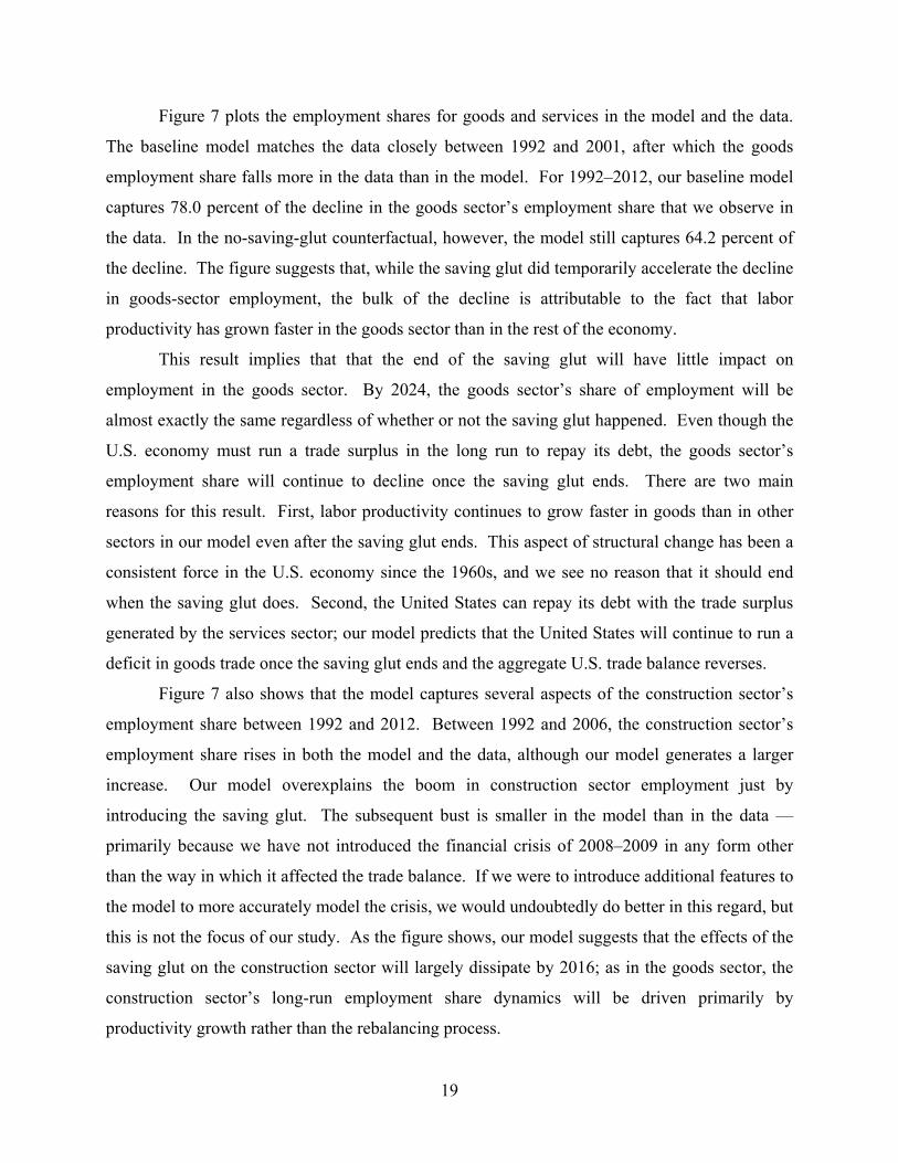
Figure 7 plots the employment shares for goods and services in the model and the data.

The baseline model matches the data closely between 1992 and 2001, after which the goods

employment share falls more in the data than in the model. For 1992–2012, our baseline model

captures 78.0 percent of the decline in the goods sector’s employment share that we observe in

the data. In the no-saving-glut counterfactual, however, the model still captures 64.2 percent of

the decline. The figure suggests that, while the saving glut did temporarily accelerate the decline

in goods-sector employment, the bulk of the decline is attributable to the fact that labor

productivity has grown faster in the goods sector than in the rest of the economy.

This result implies that that the end of the saving glut will have little impact on

employment in the goods sector. By 2024, the goods sector’s share of employment will be

almost exactly the same regardless of whether or not the saving glut happened. Even though the

U.S. economy must run a trade surplus in the long run to repay its debt, the goods sector’s

employment share will continue to decline once the saving glut ends. There are two main

reasons for this result. First, labor productivity continues to grow faster in goods than in other

sectors in our model even after the saving glut ends. This aspect of structural change has been a

consistent force in the U.S. economy since the 1960s, and we see no reason that it should end

when the saving glut does. Second, the United States can repay its debt with the trade surplus

generated by the services sector; our model predicts that the United States will continue to run a

deficit in goods trade once the saving glut ends and the aggregate U.S. trade balance reverses.

Figure 7 also shows that the model captures several aspects of the construction sector’s

employment share between 1992 and 2012. Between 1992 and 2006, the construction sector’s

employment share rises in both the model and the data, although our model generates a larger

increase. Our model overexplains the boom in construction sector employment just by

introducing the saving glut. The subsequent bust is smaller in the model than in the data —

primarily because we have not introduced the financial crisis of 2008–2009 in any form other

than the way in which it affected the trade balance. If we were to introduce additional features to

the model to more accurately model the crisis, we would undoubtedly do better in this regard, but

this is not the focus of our study. As the figure shows, our model suggests that the effects of the

saving glut on the construction sector will largely dissipate by 2016; as in the goods sector, the

construction sector’s long-run employment share dynamics will be driven primarily by

productivity growth rather than the rebalancing process.

20

Welfare implications of the saving glut

Did the saving glut make U.S. households better off? To answer this question, we construct a

measure of real income in 1992 denominated in 1992 U.S. dollars. This real income index is the

cost of achieving the equilibrium sequence of utility from 1992 onward in units of the U.S. CPI

in 1992:

(15) 1

1992 1992( )us usht

s gt gt st st tus

t tt s

ush us us usp c p cq w

.

The prices and quantities in (15) represent equilibrium objects in our benchmark model. To

convert this object to 1992 dollars, we scale it so that consumption expenditures in the model are

equal to 1992 private consumption in the national income and product account (NIPA) tables.

We use the resulting scaling factor to calculate real income in alternative scenarios, like the

counterfactual in which the saving glut does not occur or the scenario in which both the saving

glut and a sudden stop occur.

In our baseline model we assume that, in 1992, model agents expect government

consumption expenditures to remain fixed at the 1992 level of 16.6 percent of GDP, but when

the saving glut begins, an unforeseen change in government spending policy occurs:

Government spending as a fraction of GDP tracks the data between 1993 and 2012, then rises to

22.9 percent over time. This reflects policy changes that have occurred over the past two

decades, such as increased health care and defense spending, that people likely did not anticipate

in the early 1990s. This increase in government consumption gives U.S. households an incentive

to save for the future. We report our welfare results under an alternative assumption: In 1992,

agents expect government consumption, as a fraction of GDP, to follow the path it actually took

between 1992 and 2012, and then follow the same trajectory to 22.9 percent that we used in the

saving-glut scenario in our main exercise. In the saving-glut scenario, we require that

government consumption, in terms of actual quantities of goods and services, stay constant in all

three stages of the exercise: the no-saving-glut counterfactual, the saving glut with gradual

rebalancing, and the sudden stop. This modification has virtually no impact on any of the results

reported above, and it allows for direct welfare comparisons across the three scenarios even if

government spending enters the utility function — as long as it enters in an additively separable

fashion — allowing us to ask whether the saving glut is good or bad, and just how costly a

sudden stop would be.

21

The first column of table 3 presents our results on the welfare impact of the saving glut

for our baseline model. In row 1, column 1, we report real income of U.S. households in 1992

relative to the gradual rebalancing scenario. Our model indicates that the real income of U.S.

households in 1992 would have been $689 billion lower if the saving glut had never occurred:

10.9 percent of U.S. GDP in 1992. Twenty years of increased consumption of foreign imports

have made U.S. households substantially better off — as long as the saving glut ends in gradual

rebalancing.

6. Sensitivity analysis

We have performed extensive sensitivity analysis with our model. Our main results about the

reallocation of labor across sectors are robust to all the modeling alternatives that we have tried.

In this section, we discuss five modeling alternatives in detail: (1) We allow the savings glut to

end abruptly in a sudden stop. (2) We relax our baseline model’s assumption of perfect foresight

by studying a version of our model in which the duration of the saving glut is uncertain — rwt

now follows a stochastic process — and agents have rational expectations. (3) We remove the

input-output relationships between sectors. (4) We do not allow services to be traded

internationally. (5) We calibrate the preferences of U.S. households, rather than those of

households in the rest of the world, to generate observed U.S. borrowing — a domestic saving

drought instead of a global saving glut.

Alternative endings to the savings glut

In the baseline model, the rebalancing process is gradual and orderly. In this section, we use our

model to explore the implications of a sudden end to the savings glut.

We model a sudden stop to capital inflows in 2015–2016 as a surprise. Agents in the

model have perfect foresight before and after the sudden stop, but when the sudden stop occurs,

it is completely unexpected. We model the sudden stop as a surprise because U.S. interest rates

currently indicate that financial markets do not assign a significantly positive probability to a

U.S. debt crisis — just as they did not assign significantly positive probabilities to a crisis in

Mexico in 1995 or to the currently ongoing debt crises in the Eurozone. (See, for example,

Arellano, Conesa, and Kehoe, 2012.) We think of the possibility of a debt crisis striking the

22

United States as the sort of self-fulfilling crisis modeled by Cole and Kehoe (2000) and Conesa

and Kehoe (2012).

We model a sudden stop as a two-year period during which the United States is restricted

from borrowing further from the rest of the world, after which foreigners are again willing to

purchase U.S. bonds. We assume that the rest of the world’s preference parameter rwt

converges to its long-run value of 1 more quickly than in the previous scenario to capture the

idea that a sudden stop is associated with a faster end to the forces that drove the saving glut.

Furthermore, we assume that a sudden stop generates a disorderly adjustment in financial

markets that causes total factor productivity (TFP) in all three production sectors to fall by 10

percent in 2015, to recover half of this drop in 2016, and to fully recover in 2017. This TFP drop

captures the sort of disruption and rapid recovery that occurred in sudden stop episodes like that

in Mexico in 1995–1996. We also assume that the U.S. government’s debt as a fraction of GDP

falls to a lower long-run level (60 percent) than in the baseline model, representing the idea that a

sudden stop is associated with, or perhaps triggers, a long-term change in U.S. government debt

policy.

The sudden stop triggers an immediate reversal in capital flows and a large real exchange

rate depreciation. The trade balance rises from −1.5 percent of GDP to 2.8 percent on impact,

and the real exchange rate depreciates by 12.7 percent. The trade balance reversal induces the

goods sector’s labor compensation share to rise from 14.3 percent to 15.1 percent on impact.

These effects, however, would be short-lived. By 2024 the trade balance and real exchange rate

would be almost identical to their levels in the gradual rebalancing scenario. Although a sudden

stop involves quicker debt repayment, the effect on the long-term need to repay is small in our

model. The United States has borrowed so much from the rest of the world in the last two

decades that two years of rapid repayment do not make much of a dent in the overall stock of

debt.

We report the welfare effects of a sudden stop in table 3. If the savings glut ends in a

sudden stop, the real income of U.S. households will fall by $1,019 billion compared with the

baseline model: If the saving glut ends in a sudden stop rather than gradual rebalancing, U.S.

households would have been better off if the saving glut had never occurred. We also report

welfare in a version of our model in which a sudden stop occurs but TFP does not fall. In this

case, welfare falls by only $386 billion— a sudden stop without an accompanying TFP shock

23

would be painful, but would not completely wipe out the welfare gains generated by the saving

glut.

Stochastic saving glut

In our baseline model, agents in both the United States and the rest of the world have perfect

foresight once the saving glut begins: They know exactly when it will end and the rate at which

it will rebalance. We have also run numerical experiments with a model in which there is

uncertainty about the length of the saving glut and model agents have rational expectations. In

this version of the model, once the saving glut begins, in each year 1993–2011, there is a 10

percent chance that the saving glut will end in the following year, and the rest of the world’s

demand for saving will begin to decrease. The other 90 percent of the time, the saving glut will

continue into the next year. The realized path the economy takes is the one in which the saving

glut persists through 2012, and, while this is unconditionally the most likely path the economy

can take, it is not very likely from the perspective of agents in 1992. Our experiments indicate

that this kind of uncertainty has no discernible impact on our results, so we do not report them

here.

The introduction of uncertainty into our model represents a substantial technical

departure from our baseline model. Due to the presence of asymmetric, time-varying growth

rates in productivity, demographics, and other variables, our modeling framework does not admit

a stationary dynamic program. In the model with uncertainty, the current value of the stochastic

saving-glut process is not a sufficient statistic for the exogenous state of the economy — the

entire history of shocks matters. As a consequence, we must solve for the growth paths of the

world economy along all possible sequences of shocks simultaneously. The number of possible

sequences increases in proportion to the number of periods with uncertainty, so the

dimensionality of the problem increases rapidly. Although the introduction of uncertainty does

not have a significant impact on our results in this paper, the stochastic model should be useful in

other contexts.

24

No input-output production structure

In our baseline model, goods and services are used as intermediate inputs as well as

consumption, but models in the closed economy structural change literature typically abstract

from intermediate goods. Here we use a version of our model without intermediate inputs to

demonstrate the importance of this feature in accounting for structural change. To do so, we set

all of the intermediate input values in the input-output matrix to zero, and then adjust the

remainder of the matrix so that it is once again consistent with the national accounts and sectoral

labor compensation data for 1992. We then recalibrate our model and perform the same

quantitative exercises as before.

Removing the input-output structure from the model has little impact on our model’s

predictions for the disaggregated trade balances or the real exchange rate, so we focus on the

employment results, which we report in figure 8. In the no-saving-glut scenario (the dashed lines

in figure 8), the goods sector’s labor share in the model without intermediate inputs falls less

than in the model with intermediate inputs: Differential sectoral productivity growth has a much

smaller effect on goods-sector employment when production does not require intermediate

inputs. The intuition for this result lies in the substitutability of goods and services in both

intermediate and final uses. The elasticity of substitution between goods and services in

intermediate use is zero (Leontief production), while the elasticity in consumption is 0.5. When

we remove intermediate inputs, the overall elasticity of substitution in both final and

intermediate uses rises substantially, lowering the amount of reallocation of labor from goods to

services in the long run.

In the model with the savings glut (the solid lines), removing intermediate inputs leads us

to attribute a much larger decline in goods-sector employment to the saving glut than we do in

the baseline model. Relative to the no-savings-glut scenario, goods-sector employment falls and

then recovers more when production does not require intermediate inputs. This result is also a

function of the substitutability of goods and services. Goods and services become more

substitutable in the model without intermediate goods, so agents can make a larger shift into

services and away from the less-needed domestic goods.

25

Nontradable services

Here we study how our results change when we adopt the standard modeling convention in

which services are nontradable. We recalibrate our model as in the previous section so that the

goods sector is responsible for total U.S. imports and exports in 1992 and then perform the same

quantitative exercises described above.

In the no-saving-glut counterfactual, ignoring services trade has no impact on the goods

sector’s labor compensation share in the short or long run. Once we introduce the saving glut,

however, ignoring services trade makes the goods sector’s labor compensation share fluctuate

more. When the U.S. trade deficit rises between 1992 and 2006, the goods sector’s employment

share falls from 19.7 percent to 14.2 percent in the no-services-trade version of the model, versus

14.6 percent in the baseline model. Once the U.S. trade deficit begins to fall in 2007, there is a

larger temporary recovery in goods-sector employment in the no-services-trade model, since the

United States must run a trade surplus in goods to repay its debt. By 2024, however, the goods

sector’s employment share is on almost the same trajectory in both the no-services-trade and

baseline models. Services trade is quantitatively important in explaining the impact of the saving

glut on goods-sector employment over the past two decades, but it is not important in explaining

longer-term trends in structural change.

Domestic saving drought

In our baseline model, we have adopted the global-saving-glut hypothesis proposed by Bernanke

(2005), which posits that U.S. borrowing from the rest of the world since the early 1990s has

been driven primarily by increased demand for saving in the rest of the world. A number of

other authors, such as Chinn and Ito (2007), Gruber and Kamin (2007), and Obstfeld and Rogoff

(2009), argue that domestic factors such as monetary policy, housing market policy, and

innovations in financial markets were the primary cause of U.S. borrowing. In this section, we

study a version of our model in which the preferences of U.S. households, rather than the

preferences of households in the rest of the world, drive the U.S. trade balance. Following Chinn

and Ito (2007), we refer to this version of the model as the domestic-saving-drought model. In

the saving-drought model, the preferences of U.S. households take the same form as in (10) and

26

we calibrate the U.S. preference parameter ust so that the model matches the U.S. trade balance

exactly during 1992–2012, after which it gradually converges to its long-run level ofone.

To assess which of the models is more consistent with the data, we focus on investment.

Figure 9 shows that, before the financial crisis of 2009, U.S. investment rose steadily as a

fraction of GDP. This is consistent with the saving-glut theory: U.S. households took advantage

of cheap foreign goods to increase both investment and consumption, since the relative value

they placed on future consumption remained unchanged. If U.S. borrowing was instead driven

by reduced demand for saving in the United States, U.S. households should have reduced

investment in favor of increased consumption. Figure 9 shows that, except for the year 1993,

investment in the baseline model moves in the same direction as the data. By contrast,

investment in the saving-drought model falls dramatically beginning in 1997 while it continues

to rise in the data (except during the 2001 recession, which we have not attempted to incorporate

into the model). During the financial crisis of 2008–2009 (which we have modeled solely

through the increasing trade balance), investment falls in the baseline model and the data, but

rises in the saving-drought model. Overall, the correlation between investment in the saving-glut

model and the data in first differences is 0.7; the same correlation between investment in the

saving-drought model and the data is −0.6.

7. Directions for future research and concluding remarks

We have developed a model of the United States and the rest of the world and have shown that,

when we incorporate increased foreign borrowing and productivity growth in the goods sector

that is faster than in services and construction, the model accounts for three key facts about the

U.S. economy during 1992–2012: (1) The real exchange rate appreciated, then depreciated; (2)

the trade balance dynamics are driven almost entirely by the goods trade balance; and (3) labor

shifted away from the goods sector toward services and construction. We use our model to show

that while the faster productivity growth in the goods sector is responsible for the long-run shift

in employment away from the goods sector, the saving glut strengthened this effect during 1992–

2012.

Although the savings glut’s impact on goods-sector employment is temporary, this does

not imply that the saving glut has not had a major long-run impact on the U.S. economy: The

U.S. economy’s current long-run trajectory is very different from the one it would have taken

27

had the saving glut not occurred. Figures 4 and 5 illustrate this point by plotting the aggregate

trade balance and real exchange rate in our gradual rebalancing scenario against the

counterfactual in which the saving glut never happened. In the counterfactual, U.S. trade is

approximately balanced in the long run, since the United States has little debt to repay. Because

the saving glut did happen, however, our model predicts that the United States will have to run a

trade surplus of around 1 percent of GDP in perpetuity. To do so, the U.S. real exchange rate

will depreciate by about 6 percent compared with what it would have been if the saving glut had

not taken place.

Our analysis identifies two puzzles. Here we discuss these puzzles and point out

directions that future research could take in addressing them.

The first puzzle is: Why did U.S. borrowing continue to increase once the U.S. real

exchange rate began to depreciate? In other words, why did U.S. purchases of foreign goods and

services continue to increase once foreign goods and services stopped getting cheaper and started

getting more expensive, as seen in the data in figure 3? A partial resolution to this puzzle might

be found in the J-curve literature (Backus, Kehoe, and Kydland, 1994), in that time-to-build and

import pattern adjustment frictions can delay quantities adjusting to price changes. This

mechanism is not likely to explain the substantial four-year lag, however. A more plausible

resolution to the puzzle is the increase in the importance of China in U.S. borrowing during the

period. In figure 10 we decompose the U.S. real exchange rate into the real exchange rates with

China and with the United States’ other major trade partners. We see that the overall real

exchange rate and the exchange rate with non-China countries move closely in the early part of

the period, but diverge in the latter part. Following 2002, the aggregate real exchange rate

behaves much like the real exchange rate with China. Incorporating the increasing importance of

China into our model is not simply a matter of changing weights in our real exchange rate.

Instead, it would involve distinguishing between the countries that have purchased the bulk of

U.S. bonds during the saving glut, like China, Japan, and Korea, and those that have run more

balanced trade with the United States. To accurately capture this, we would need to model a

world with (at least) three countries and some sort of asset market segmentation, where countries

like China choose to lend to the United States rather than to other countries.

The second puzzle is that, in contrast to Bernanke’s (2005) judgment, the saving glut has

had only a small effect on U.S. interest rates in the model, as seen in figure 11. The largest fall

28

in the U.S. real interest rate in the model with the saving glut over 1992–2012, compared with

the model with no saving glut, is 44 basis points (3.70 percent per year compared with 3.26

percent) in 2009. This is in line with Greenspan’s (2005) judgment that foreign lending

accounted for less than 50 basis points of the drop in interest rates. Warnock and Warnock

(2009) have estimated that foreign lending drove down U.S. real interest rates by a somewhat

larger amount, about 80 basis points, throughout the period. Krishnamurthy and Vissing-

Jorgensen (2007) provide similar estimates.

In our model, the impact of the saving glut on interest rates depends on how substitutable

foreign goods are for U.S. goods. With the Armington elasticities that we have chosen, we find

that the saving glut generates the right magnitude of appreciation of the U.S. real exchange rate

in figure 5, but not the right magnitude in the drop in the U.S. real interest rate in figure 11. If

we make foreign goods more substitutable for U.S. goods, we can generate more of a drop in the

U.S. real interest rate in 2006–2012 — although still nowhere near as large as the drop observed

in the data — but the model would then predict a much smaller appreciation in the U.S. real

exchange rate.

Notice that in figure 11, our model predicts that the U.S. interest rate is driven up by

appreciation of the dollar and is driven down by depreciation. The falling prices of foreign

goods during 1993–2006 induce U.S. households to increase consumption faster than they do in

the model without a saving glut, generating the observed trade deficit. The first-order conditions

for utility maximization imply that U.S. households are willing to do this only if interest rates are

higher. As the dollar depreciates during 2006–2012, consumption grows more slowly than in the

no-saving-glut model and interest rates are lower.

Since our model’s results contradict Bernanke’s (2005) reasoning that the saving glut is

responsible for the low level of U.S. interest rates in the early 2000s, it is worth examining how

the saving glut is compatible with high interest rates in the United States. Consider the interest

rate parity condition that makes households in the rest of the world indifferent between holding

U.S. bonds and the rest of the world’s bonds:

(16) 11 11 (1 )us rw t

t tt

rerr r

rer

.

As the demand for savings increases in the rest of the world, the interest rate there increases. At

the same time, the fall in the relative price of goods in the rest of the world causes the U.S. real

29

exchange rate to appreciate, that is, to fall. Our interest rate parity condition does not pin down

the direction of change in the U.S. interest rate; in principle, it could go up or down. What tells

us that the interest rate is higher in the saving-glut model than it is in the no-saving-glut model is

the requirement that the saving glut generates the observed increase in the U.S. trade deficit,

which implies that consumption in the United States increases faster during the saving glut than

it would have with no saving glut.

To account for the very low U.S. interest rates seen in the data, we need to look

elsewhere, possibly to the sorts of U.S. policies discussed by Obstfeld and Rogoff (2009) and

Bernanke et al. (2011). It is worth pointing out, however, that modeling the source of the global

imbalances over 1992–2012 as being generated by U.S. savings behavior does not work well.

The domestic-saving-drought model is successful in generating lower U.S. interest rates during

1993–2006, as the dollar appreciates, but it generates higher U.S. interest rates during 2006–

2012, as the dollar depreciates. The low interest rates during the entire period pose a puzzle for

both models.

30

References

Acemoglu, D., and V. Guerrieri (2008), “Capital Deepening and Nonbalanced Economic Growth,” Journal of Political Economy, 116, 467–498.

Arellano, C., J. C. Conesa, and T. J. Kehoe (2012), “Chronic Sovereign Debt Crises in the Eurozone, 2010–2012,” Federal Reserve Bank of Minneapolis Economic Policy Paper 12-4.

Backus, D. K., E. Henriksen, F. Lambert, and C. Telmer (2006), “Current Account Fact and Fiction,” Unpublished manuscript, Stern School of Business, New York University, University of Oslo, and Tepper School of Business, Carnegie Mellon University.

Backus, D. K., P. J. Kehoe, and F. E. Kydland (1994), “Dynamics of the Trade Balance and the Terms of Trade: The J-Curve?” American Economic Review, 84, 84–103.

Baumol, W. J. (1967), “Macroeconomics of Unbalanced Growth: The Anatomy of Urban Crisis.” American Economic Review, 57, 415–426.

Bems, R. (2008), “Aggregate Investment Expenditures on Tradable and Nontradable Goods,” Review of Economic Dynamics, 11, 852–883.

Bernanke, B. S. (2005), “The Global Saving Glut and the U.S. Current Account Deficit,” speech at the Sandridge Lecture, Virginia Association of Economists, Richmond, VA, March 10.

Bernanke, B. S., C. Bertaut, L. P. DeMarco, and S. Kamin (2011), “International Capital Flows and the Returns to Safe Assets in the United States, 2003-2007,” Board of Governors of the Federal Reserve System International Finance Discussion Paper 1014.

Bivens, J. (2006), “Trade Deficits and Manufacturing Job Loss; Correlation and Causality,” EPI Briefing Paper 171.

Buera, F. J., and J. P. Kaboski (2009), “Can Traditional Theories of Structural Change Fit the Data?” Journal of the European Economic Association, 7, 467–477.

Buera, F. J., and J. P. Kaboski (2012), “The Rise of the Service Economy,” American Economic Review, 102, 2540–69.

Caballero, R. J., E. Farhi, and P.-O. Gourinchas (2008), “An Equilibrium Model of ‘Global Imbalances’ and Low Interest Rates,” American Economic Review, 98, 358–393.

Calvo, G. A., A. Izquierdo, and L.-F. Mejía (2004), “On the Empirics of Sudden Stops: The Relevance of Balance-Sheet Effects,” NBER Working Paper 10520.

Calvo, G. A., and E. Talvi (2005), “Sudden Stop, Financial Factors and Economic Collapse in Latin America: Learning from Argentina and Chile,” NBER Working Paper 11153.

31

Chinn, M. D., and H. Ito (2007), “Current Account Balances, Financial Development and Institutions: Assaying the World ‘Saving Glut’,” Journal of International Money and Finance, 26, 546–569.

Cole, H. L., and T. J. Kehoe (2000), “Self-Fulfilling Debt Crises,” Review of Economic Studies, 67, 91–116.

Conesa, J. C., and T. J. Kehoe (2012), “Gambling for Redemption and Self-Fulfilling Debt Crises,” Federal Reserve Bank of Minneapolis Staff Report 465.

Du, Q., and S. Wei (2013), “A Theory of the Competitive Saving Motive,” NBER Working Paper 18911.

Echevarria, C. (1995), “Agricultural Development vs. Industrialization; Effects of Trade,” Canadian Journal of Economics, 28, 631–647.

Gourinchas, P.-O., and H. Rey (2007), “From World Banker to World Venture Capitalist: U.S. External Adjustment and the Exorbitant Privilege,” in R. H. Clarida, ed., G7 Current Account Imbalances: Sustainability and Adjustment, University of Chicago Press, 11–66.

Greenspan, A. (2005), “Monetary Policy Report to the Congress,” statement before the Committee on Banking, Housing and Urban Affairs, U.S. Senate, February 16.

Gruber, J. W., and S. B. Kamin (2007), “Explaining the Global Pattern of Current Account Imbalances,” Journal of International Money and Finance, 26, 500–522.

Jin, K. (2012), “Industrial Structure and Capital Flows,” American Economic Review, 102, 2111–2146.

Kehoe, T. J., and K. J. Ruhl (2009), “Sudden Stops, Sectoral Reallocations, and the Real Exchange Rate,” Journal of Development Economics, 89, 235–249.

Kongsamut, P., S. Rebelo, and D. Xie (2001), “Beyond Balanced Growth,” Review of Economic Studies, 68, 869–882.

Krishnamurthy, A., and A. Vissing-Jorgensen (2007), “The Demand for Treasury Debt,” NBER Working Paper 12881.

Lane, P. R., and G. M. Milesi-Ferretti (2007), “The External Wealth of Nations Mark II: Revised and Extended Estimates of Foreign Assets and Liabilities, 1970–2004,” Journal of Monetary Economics, 73, 223–250.

Lane, P. R., and G. M. Milesi-Ferretti (2008), “Where Did All the Borrowing Go? A Forensic Analysis of the U.S. External Position,” IMF Working Paper WP/08/28.

Matsuyama, K. (1992), “Agricultural Productivity, Comparative Advantage, and Economic Growth,” Journal of Economic Theory, 58, 317–334.

32

Matsuyama, K. (2009), “Structural Change in an Interdependent World: A Global View of Manufacturing Decline,” Journal of the European Economic Association, 7, 478–486.

Mendoza, E. G., V. Quadrini, and J.-V. Ríos-Rull (2009), “Financial Integration, Financial Development, and Global Imbalances,” Journal of Political Economy, 117, 371–416.

Miller, R. E., and P. D. Blair (2009), Input-Output Analysis: Foundations and Extensions, 2nd ed., Cambridge University Press.

Ngai, L. R., and Pissarides, C. A. (2007), “Structural Change in a Multisector Model of Growth,” American Economic Review, 97, 429–443.

Obstfeld M., and K. Rogoff (2005), “Global Current Account Imbalances and Exchange Rate Adjustments,” Brookings Papers on Economic Activity 1, 67–146. Obstfeld, M., and K. Rogoff (2007), “The Unsustainable U.S. Current Account Position Revisited,” in R. H. Clarida, ed., G7 Current Account Imbalances: Sustainability and Adjustment, University of Chicago Press, 339–376.

Obstfeld, M., and K. Rogoff (2009), “Global Imbalances and the Financial Crisis: Products of Common Causes,” CEPR Discussion Paper 7606.

Perri, F., and A. Fogli (2010), “Macroeconomic Volatility and External Imbalances,” Unpublished manuscript, University of Minnesota.

Ruhl, K. J. (2008), “The International Elasticity Puzzle,” Unpublished manuscript, NYU Stern School of Business.

Scott, R. E., H. Jorgensen, and D. Hall (2013), “Reducing U.S. Trade Deficits Will Generate a Manufacturing-Based Recovery for the United States and Ohio,” EPI Briefing Paper 351.

Sevaldson, P. (1970), “The Stability of Input-Output Coefficients,” in A. P. Carter and A. Brody, eds., Applications of Input-Output Analysis, North-Holland, 207–237.

Sposi, M. (2012), “Evolving Comparative Advantage, Structural Change, and the Composition of Trade,” Unpublished manuscript, University of Iowa.

Stockman, A. C., and L. L. Tesar (1995), “Tastes and Technology in a Two-Country Model of the Business Cycle: Explaining International Comovements,” American Economic Review, 85, 168–185.

United Nations (2011), World Population Prospects: The 2010 Revision, Vol. 1: Comprehensive Tables, http://esa.un.org/unpd/wpp/Documentation/pdf/WPP2010_Volume-I_Comprehensive-Tables.pdf.

33

U.S. Congress, Congressional Budget Office (2012), The 2012 Long-Term Budget Outlook, http://www.cbo.gov/sites/default/files/cbofiles/attachments/06-05-Long_Term_Budget-Outlook_2.pdf.

Warnock, F. E., and V. C. Warnock (2009), “International Capital Flows and U.S. Interest Rates,” Journal of International Money and Finance, 28, 903–919.

Uy, T., K.-M. Yi, and J. Zhang (2013), “Structural Change in an Open Economy,” Unpublished manuscript, University of Minnesota, Federal Reserve Bank of Minneapolis, University of Michigan.

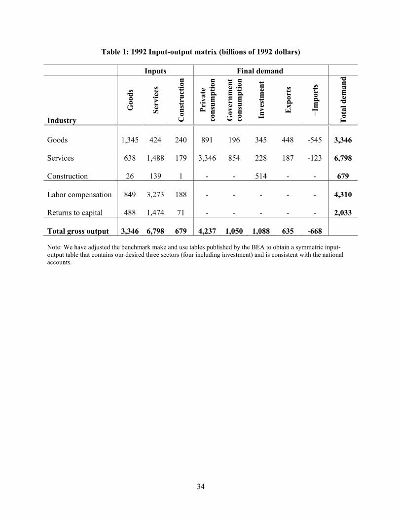
34

Table 1: 1992 Input-output matrix (billions of 1992 dollars)

Inputs Final demand

Industry G

ood

s

Ser

vice

s

Con

stru

ctio

n

Pri

vate

co

nsu

mp

tion

Gov

ern

men

t co

nsu

mp

tion

Inve

stm

ent

Exp

orts

−Im

por

ts

Tot

al d

eman

d

Goods

1,345

424

240

891

196

345

448 -545

3,346

Services

638

1,488

179

3,346

854

228

187 -123

6,798

Construction

26

139

1

-

-

514 - -

679

Labor compensation

849

3,273

188

-

-

- - -

4,310

Returns to capital

488

1,474

71

-

-

- - -

2,033

Total gross output

3,346

6,798

679

4,237

1,050

1,088

635 -668 Note: We have adjusted the benchmark make and use tables published by the BEA to obtain a symmetric input-output table that contains our desired three sectors (four including investment) and is consistent with the national accounts.

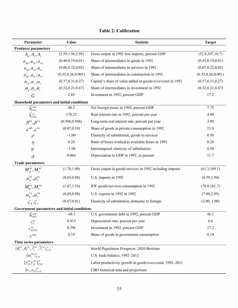
35

Table 2: Calibration

Parameter Value Statistic Target

Producer parameters

, ,g s cA A A (2.59,1.56,2.95) Gross output in 1992 less imports, percent GDP (52.8,107,10.7)

, ,gg sg cga a a (0.40,0.19,0.01) Share of intermediates in goods in 1992 (0.41,0.19,0.01)

, ,gs ss csa a a (0.06,0.22,0.02) Share of intermediates in services in 1992 (0.07,0.22,0.02)

, ,gc sc cca a a (0.35,0.26,0.001) Share of intermediates in construction in 1992 (0.35,0.26,0.001)

, ,g s c (0.37,0.31,0.27) Capital’s share of value added in goods/svcs/const in 1992 (0.37,0.31,0.27)

, ,g s c (0.32,0.21,0.47) Share of intermediates in investment in 1992 (0.32,0.21,0.47)

G 2.85 Investment in 1992, percent GDP 17.2

Household parameters and initial conditions

1992ushb 40.3 Net foreign assets in 1992, percent GDP 7.75

1992usk 176.25 Real interest rate in 1992, percent per year 4.00

,us rw (0.996,0.996) Long-term real interest rate, percent per year 3.00

,ush rw (0.07,0.19) Share of goods in private consumption in 1992 21.0

-1.00 Elasticity of substitution, goods to services 0.50

0.28 Ratio of hours worked to available hours in 1992 0.29

-1.00 Intertemporal elasticity of substitution 0.50

0.066 Depreciation to GDP in 1992, in percent 11.7

Trade parameters

,us usg sM M (1.78,1.09) Gross output in goods/services in 1992 including imports (61.3,109.1)

,us usg s (0.65,0.98) U.S. imports in 1992 (8.59,1.94)

,rw rwg sM M (1.67,1.10) RW goods/services consumption in 1992 (78.0,161.7)

,rw rwg s (0.69,0.98) U.S. exports in 1992 in 1992 (7.06,2.95)

,g s (0.67,0.01) Elasticity of substitution, domestic to foreign (3.00, 1.00)

Government parameters and initial conditions

1992usgb -48.1 U.S. government debt in 1992, percent GDP 48.1

usk 0.415 Depreciation rate, percent per year 6.6

1993usk 0.396 Investment in 1992, percent GDP 17.2

usg 0.19 Share of goods in government consumption 0.19

Time series parameters

0{ , , , }us rw us rwt t t t tn n

World Population Prospects: 2010 Revision

0{ }rwt t

U.S. trade balance, 1992–2012

0{ }us rwjt jt t

Labor productivity growth in goods/svcs/const, 1992–2011

0{ , }t t t CBO historical data and projections

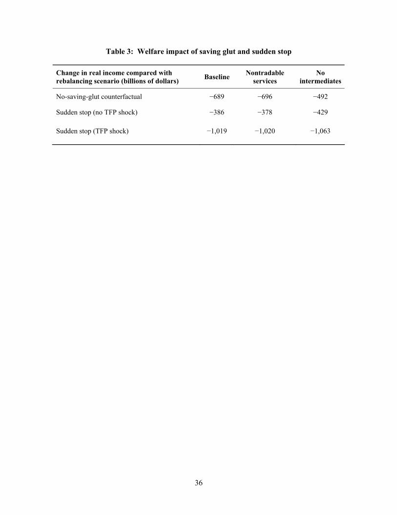
36

Table 3: Welfare impact of saving glut and sudden stop

Change in real income compared with rebalancing scenario (billions of dollars) Baseline Nontradable

services No

intermediates

No-saving-glut counterfactual −689 −696 −492

Sudden stop (no TFP shock) −386 −378 −429

Sudden stop (TFP shock) −1,019 −1,020 −1,063

37

Figure 1: U.S. trade balance vs. goods sector’s employment share

Figure 2: Labor productivity in goods, services, and construction

38

Figure 3: U.S. trade balance, current account balance, and real exchange rate

Figure 4: U.S. trade balance in the model and the data

39

Figure 5: U.S. real exchange rate in the model and the data

Figure 6: Disaggregated trade balances in the model and the data

Figure 7: Goods and construction employment shares in the model and the data

40

Figure 8: Goods employment share in no-input-output model vs. baseline model

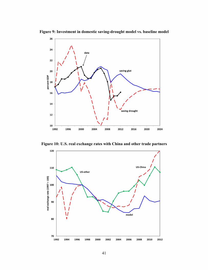
41

Figure 9: Investment in domestic saving-drought model vs. baseline model

Figure 10: U.S. real exchange rates with China and other trade partners

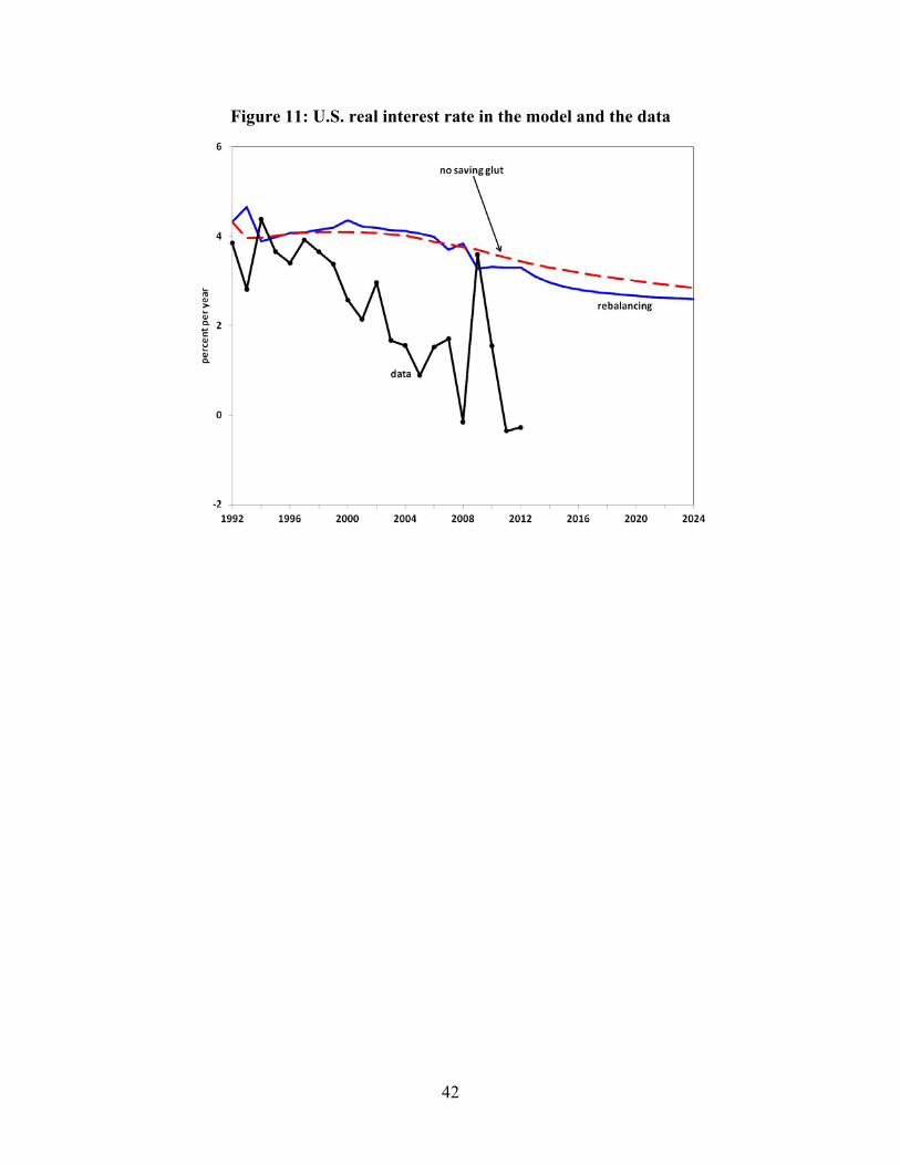
42

Figure 11: U.S. real interest rate in the model and the data