Global illumination with radiance regression functions

ACM Reference FormatRen, P., Wang, J., Gong, M., Lin, S., Tong, X., Guo, B. 2013. Global Illumination with Radiance Regression Functions. ACM Trans. Graph. 32, 4, Article 130 (July 2013), 12 pages. DOI = 10.1145/2461912.2462009 http://doi.acm.org/10.1145/2461912.2462009.

Copyright NoticePermission to make digital or hard copies of all or part of this work for personal or classroom use is granted without fee provided that copies are not made or distributed for profi t or commercial advantage and that copies bear this notice and the full citation on the fi rst page. Copyrights for components of this work owned by others than ACM must be honored. Abstracting with credit is permitted. To copy otherwise, or republish, to post on servers or to redistribute to lists, requires prior specifi c permission and/or a fee. Request permis-sions from [email protected] © ACM 0730-0301/13/07-ART130 $15.00.DOI: http://doi.acm.org/10.1145/2461912.2462009

Global Illumination with Radiance Regression Functions

Peiran Ren∗‡ Jiaping Wang† Minmin Gong‡ Stephen Lin‡ Xin Tong‡ Baining Guo‡∗∗Tsinghua University † Microsoft Corporation ‡ Microsoft Research Asia

(c)(a) (b)

Figure 1: Real-time rendering results with radiance regression functions for scenes with glossy interreflections (a), multiple local lights (b),and complex geometry and materials (c).

Abstract

We present radiance regression functions for fast rendering ofglobal illumination in scenes with dynamic local light sources. Aradiance regression function (RRF) represents a non-linear map-ping from local and contextual attributes of surface points, such asposition, viewing direction, and lighting condition, to their indirectillumination values. The RRF is obtained from precomputed shad-ing samples through regression analysis, which determines a func-tion that best fits the shading data. For a given scene, the shadingsamples are precomputed by an offline renderer.

The key idea behind our approach is to exploit the nonlinear co-herence of the indirect illumination data to make the RRF bothcompact and fast to evaluate. We model the RRF as a multilayeracyclic feed-forward neural network, which provides a close func-tional approximation of the indirect illumination and can be effi-ciently evaluated at run time. To effectively model scenes with spa-tially variant material properties, we utilize an augmented set ofattributes as input to the neural network RRF to reduce the amountof inference that the network needs to perform. To handle sceneswith greater geometric complexity, we partition the input space ofthe RRF model and represent the subspaces with separate, smallerRRFs that can be evaluated more rapidly. As a result, the RRFmodel scales well to increasingly complex scene geometry and ma-terial variation. Because of its compactness and ease of evaluation,the RRF model enables real-time rendering with full global illu-mination effects, including changing caustics and multiple-bouncehigh-frequency glossy interreflections.

CR Categories: I.3.7 [Computer Graphics]: Three-DimensionalGraphics and Realism—Color, shading, shadowing, and texture;Links: DL PDF WEB

Keywords: global illumination, real time rendering, neural net-work, non-linear regression

1 Introduction

Global light transport provides scenes with visually rich shadingeffects that are an essential component of photorealistic rendering.Much of the shading detail arises from multiple bounces of light.This reflected light, known as indirect illumination, is generally ex-pensive to compute. The most successful existing approach for in-direct illumination is precomputed radiance transfer (PRT) [Sloanet al. 2002; Ramamoorthi 2009], which precomputes the globallight transport and stores the resulting PRT data for fast render-ing at run time. However, even with PRT, real-time rendering withdynamic viewpoint and lighting remains difficult.

Two major challenges in real-time rendering of indirect illumina-tion are dealing with dynamic local light sources and handling high-frequency glossy interreflections. Most existing PRT methods as-sume that the lighting environment is sampled at a single point inthe center of the scene and the result is stored as an environmentmap. For this reason, these methods cannot accurately represent in-cident radiance of local lights at different parts of the scene. To ad-dress this problem, Kristensen et al. [2005] precomputed radiancetransfer for a dense set of local light positions and a sparse set ofmesh vertices. Their approach works well for diffuse scenes but hasdifficulty representing effects such as caustics and high-frequencyglossy interreflections, since it would be prohibitively expensive tostore the precomputed data for a dense set of mesh vertices.

To face these challenges, we introduce the radiance regressionfunction (RRF), a function that returns the indirect illuminationvalue for each surface point given the viewing direction and light-ing condition. The key idea of our approach is to design the RRFas a nonlinear function of surface point properties such that it has acompact representation and is fast to evaluate. The RRF is learnedfor a given scene using nonlinear regression [Hertzmann 2003] ontraining samples precomputed by offline rendering. These samplesconsist of a set of surface points rendered with random viewingand lighting conditions. Since the indirect illumination of a surfacepoint in a given scene is determined by its position, the location oflight sources, and the viewing direction, we define these propertiesas basic attributes of the point and learn the RRF with respect tothem. In rendering, the attributes of each visible surface point areobtained while evaluating direct illumination. The indirect illumi-

ACM Transactions on Graphics, Vol. 32, No. 4, Article 130, Publication Date: July 2013

http://doi.acm.org/10.1145/2461912.2462009

http://portal.acm.org/ft_gateway.cfm?id=2462009&type=pdf

http://shadebot.com/rrf_sig13/

nation of each point is then computed from their attributes usingthe RRF, and added to the direct illumination to generate a globalillumination solution.

We model the RRF by a multilayer acyclic feed-forward neural net-work. As a universal function approximator [Hornik et al. 1989],such a neural network can approximate the indirect illuminationfunction to arbitrary accuracy when given adequate training sam-ples. The main technical issue in designing our neural network RRFis how to achieve a good approximation through efficient use of theprecomputed training samples. To address this issue we presenttwo techniques. The first is to augment the set of attributes at eachpoint to include spatially variant surface properties. Though regres-sion could be performed using only the basic attributes, this resultsin suboptimal use of the training data and inferior approximationresults because spatially variant surface properties make the RRFhighly complex as a function of only the basic attributes. By per-forming regression with respect to an enlarged set of attributes thatincludes surface normal and material properties, the efficiency ofsample use is greatly elevated because the mapping from the aug-mented attributes to indirect illumination can be much more easilycomputed from training samples. The second technique is to par-tition the space of RRF input vectors and fit a separate RRF foreach of the subspaces. Though a single neural network can effec-tively model the indirect illumination of a simple scene, the largernetwork size needed to model complex scenes leads to substan-tially increased training and evaluation time. To expedite run-timeevaluation, we employ multiple smaller networks that collectivelyand more efficiently represent indirect illumination throughout thescene.

Our main contribution is a fundamentally new approach for real-time rendering of precomputed global illumination. Our methoddirectly approximates the indirect global illumination, which is ahighly complex and nonlinear 6D function (of surface position,viewing direction, and lighting direction). With carefully designedneural networks, our method can effectively exploit the nonlinearcoherence of this function in all six dimensions simultaneously. Bycontrast, PRT methods only exploit nonlinear coherence in somedimensions and resort to dense sampling in the other dimensions.Run-time evaluation of analytic neural-network RRFs can be ac-complished in screen space with a deferred shading pass easily in-tegrated into existing rendering pipelines. As a result, the precom-puted RRFs are both compact and fast to evaluate, and our methodcan render challenging visual effects - such as caustics, sharp in-direct shadows, and high-frequency glossy interreflections - all inreal time. In our method the precomputed neural networks dependonly on lighting effects on the object surface, not on the underlyingsurface meshing. This makes our method more scalable than PRT,which relies on dense surface meshing for high-frequency lightingeffects.

As far as we know, our method provides the first real-time solutionfor rendering full indirect illumination effects of complex sceneswith dynamic local lighting and viewing. For scenes with complexgeometry and material variations (e.g., Figure 1), our technique canrender their full global illumination effects in 512× 512 imagesat 30 FPS, capturing visual effects such as caustics (Figure 9(a)),high-frequency glossy interreflections (Figure 8(d)), glossy inter-reflections produced by four or more light bounces (Figure 1(a) andFigure 10), indirect hard shadows (Figure 1(c)), and mixtures of dif-ferent lighting effects in complex scenes (Figure 12). The renderingtime mainly depends on the screen size, not the number of objectsin the scene. It is fairly easy to scale up to larger scenes with manyobjects because our run-time algorithm renders all visible objects inparallel in screen space. This scalability is reflected in our results,where the frame rates of the complex bedroom scene (Figure 12)and the simple Cornell box (Figure 9(a)) are about the same. Our

RRF representation is run-time local, i.e., the run-time evaluationof the RRFs of each 3D object is independent of the RRFs of other3D objects in the scene.

2 Related Work

Due to space limitations, we only discuss recent methods that aredirectly related to our work. For a broader presentation on inter-active global illumination techniques, we refer the reader to recentsurveys [Wald et al. 2009; Ramamoorthi 2009; Ritschel et al. 2012].

Interactive Global Illumination Numerous methods have beenproposed to quickly compute the global illumination of a scene.One solution is to accelerate classical global illumination algo-rithms using the GPU or multiple CPUs [Wald et al. 2009]. Re-cently, Wang et al. [2009] presented a GPU based photon mappingmethod for rendering full global illumination effects. McGuire etal. [2009] developed an image space photon mapping algorithm toexploit both the CPU and GPU for global illumination. Parker etal. [2010] described a programmable ray tracing engine designedfor the GPU and other highly parallel architectures.

Another approach for obtaining real-time frame rates is to sac-rifice accuracy for speed. One such solution is to approximateindirect lighting reflected from surfaces as a set of virtual pointlights (VPLs) [Keller 1997; Dachsbacher and Stamminger 2006;Ritschel et al. 2008; Nichols and Wyman 2010; Thiedemann et al.2011]. Several methods [Dong et al. 2007; Dachsbacher et al. 2007;Crassin et al. 2011] approximate global illumination using coarse-scale solutions computed over a scene hierarchy. More recently,Kaplanyan et al. [2010] approximated low frequency indirect illu-mination in dynamic scenes by computing light propagation over a3D scene lattice. While this method is fast and compact, it can onlysimulate indirect illumination of diffuse surfaces.

Despite the different strategies used for speeding up computation,the processing costs of these methods remain proportional to thenumber of light bounces, which effectively limits the interreflec-tion effects they can simulate. As the scene geometry becomesmore complex and the material becomes more glossy, the diverselight paths often lead to greater computational costs in each bounce,which also limits the scalability of these methods. On the contrary,our method efficiently models all indirect lighting effects, includ-ing challenging effects such as caustics and high-frequency glossyinterreflections.

Precomputed Light Transport Precomputed radiance transfer(PRT) [Sloan et al. 2002; Ng et al. 2004; Ramamoorthi 2009] pre-computes the light transport of each scene point with respect toa set of basis illuminations, and uses this data at run time to re-light the scene at real-time rates. Early methods [Sloan et al. 2002;Sloan et al. 2003] support only low-frequency global illuminationeffects by encoding the light transport with a spherical harmonics(SH) basis. Later methods factorize the BRDF at each surface pointand represent the light transport with non-linear wavelets [Liu et al.2004; Wang et al. 2006] or a spherical Gaussian basis [Tsai andShih 2006; Green et al. 2006] for rendering all-frequency globalillumination. However, these methods are limited by their supportfor only distant lighting.

To support local light sources, Kristensen et al. [2005] model re-flected radiance using a 2D SH basis, with sampling at a sparseset of mesh vertices for a dense set of local light positions. Thelight space samples are compressed by clustering, while the spatialsamples are partitioned into zones and compressed using clusteredPCA. During rendering, the data sampled at nearby light sources areinterpolated to generate rendering results for a new light position.

130:2 • P. Ren et al.


Since the data is sampled over sparse mesh vertices, this methodcannot well represent caustics and other high-frequency lighting ef-fects. Also, a high-order SH basis is needed for representing view-dependent indirect lighting effects on glossy objects.

Direct-to-indirect transfer methods [Hasan et al. 2006; Wang et al.2007; Kontkanen et al. 2006; Lehtinen et al. 2008] precompute in-direct lighting with respect to the direct lighting of the scene atsampled surface locations. During rendering, the direct shading ofthe scene is first computed and then used to reconstruct the indi-rect lighting effects. Although this method can support local lightsources, the surfaces must be densely sampled to represent high-frequency indirect lighting, which leads to large storage costs andslow rendering performance.

Regression Methods Regression methods have been widelyused in graphics [Hertzmann 2003]. For example, Grzeszczuk etal. [1998] used neural networks to emulate object dynamics andgenerate physically realistic animation without simulation. Neuralnetworks also have been used for visibility computation. Dachs-bacher [2011] applied neural networks for classifying differentvisibility configurations. Nowrouzezahrai et al. [2009] fit low-frequency precomputed visibility data of dynamic objects with neu-ral networks. These visibility neural networks allow them to predictlow-frequency self-shadowing when computing the direct shadingof a dynamic scene. Finally, Meyer et al. [2007] used statisticalmethods to select a set of key points (hundreds of them) and forma linear subspace such that at run time, global illumination onlyneeds to be calculated at these key points. Although this methodgreatly reduces computation, rendering global illumination at keypoints remains time consuming.

3 Radiance Regression Functions

In this section, we first present the radiance regression function Φ

and explain how it can be obtained through regression with respectto precomputed indirect illumination data. Then we describe howto model the function Φ as a neural network ΦN and derive an ana-lytic expression for the function ΦN . After that, we discuss neuralnetwork structure and training, leaving the more technical details toAppendix A. Finally, we show a simple example of rendering withthe function ΦN .

In a static scene lit by a moving point light source, the reflectedradiance at an opaque surface point at position xp as viewed fromdirection v is described by the reflectance equation [Cohen et al.1993]:

s(xp,v, l) =∫

Ω+ρ(xp,v,vi)(n ·vi)si(xp,vi)dvi (1)

=s0(xp,v, l)+ s+(xp,v, l),

where l is the position of the point light, ρ and n denote the BRDFand surface normal at position xp, and si(xp,vi) represents the in-coming radiance at xp from direction vi. The parametric BRDFρ can be described by a closed-form function ρc with a set of re-flectance parameters a(xp) as follows:

ρ(xp,v,vi) = ρc(v,vi,a(xp)). (2)

For a spatially variant parametric BRDF, the only part that variesspatially is the parameter vector a(xp), which is represented by aset of texture maps and thus can be efficiently used in the graphicspipeline.

As shown in Equation (1), the reflected radiance s can be sepa-rated into a local illumination component s0 and indirect illumina-tion component s+ that correspond to direct and indirect lighting

respectively. As the local illumination component s0 can be effi-ciently computed by existing methods (e.g. [Donikian et al. 2006]),we focus on the indirect illumination s+ that results from incom-ing radiance contributions to si(xp,vi) of indirect lighting. Givena point light of unit intensity at position l, the function s+(xp,v, l)represents the indirect illumination component toward viewing di-rection v.

Combining Equation (1) and Equation (2), we can express the indi-rect illumination component as

s+(xp,v, l) =∫

Ω+ρc(v,vi,a(xp))(n(xp) ·vi)s+i (xp,vi)dvi (3)

where s+i (xp,vi) is the indirect component of the incoming radiancesi(xp,vi). Here we also replaced the surface normal n by n(xp) tomake explicit the fact that the surface normal n at position xp iscomputed as a function of xp. From Equation (3) we observe thatthe indirect illumination s+ may be rewritten as

s+(xp,v, l) = s+a (xp,v, l,n(xp),a(xp)), (4)

for a new function s+a with an expanded set of attributes that in-cludes the surface normal and BRDF parameter vector.

The indirect illumination s+(xp,v, l) is a well-defined functionsince for a given scene, we can perform light transport computa-tion to obtain s+ for any surface point, light position, and viewingdirection. However, s+ generally requires lengthy processing tocompute. In this work, we introduce the radiance regression func-tion Φ, which is a function that approximates s+ in the least-squaressense and is constructed such that it is compact, fast to evaluate, andhence well-suited for real-time rendering.

Approximation by Regression We treat the approximation of in-direct illumination s+ as a regression problem [Hertzmann 2003]and learn a regression function Φ from a set of training data. Inprinciple, it would be sufficient to define Φ in terms of only the setof basic attributes xp, v and l, since they describe a minimal set offactors that determine the indirect illumination at a point in a givenscene. However, the values of surface normals n and reflectanceparameters a can vary substantially over a scene area, making indi-rect illumination s+(xp,v, l) highly complex as a function of onlythe basic attributes. Defining the regression function Φ in termsof a set of augmented attributes xp, v, l, n, and a thus allows formore effective approximation of s+ by nonlinear regression, sincethe surface quantities n and a would no longer need to be inferredfrom the training data. We therefore define the radiance regressionfunction Φ at surface point p to be Φ(xp,v, l,n,a), which representsa map from R12+np to R3 where np is the number of parameters inthe spatially variant BRDF and R3 spans the three RGB color chan-nels.

The training data we use consists of a set of N input-output pairsthat sample the indirect illumination s+(xp,v, l). Each pair is calledan example, and the i-th example comprises the pair (xi,yi), wherexi = [xi

p,vi, li,ni,ai]T , yi = s+(xip,vi, li), and i = 1, ...,N. xi is the

input vector and yi is the corresponding output vector. The radi-ance regression function Φ is determined by minimizing the least-squares error:

E = ∑i||yi−Φ(xi

p,vi, li,ni,ai)||2. (5)

There may exist many functions that pass through the trainingpoints (xi,yi) and thus minimize Equation (5). A particular solu-tion might give a poor approximation of the indirect illuminations+(xp,v, l) at a new input vector (xp,v, l,n,a) unseen in the train-ing data. To produce a better approximation, a larger training set

Global Illumination with Radiance Regression Functions • 130:3


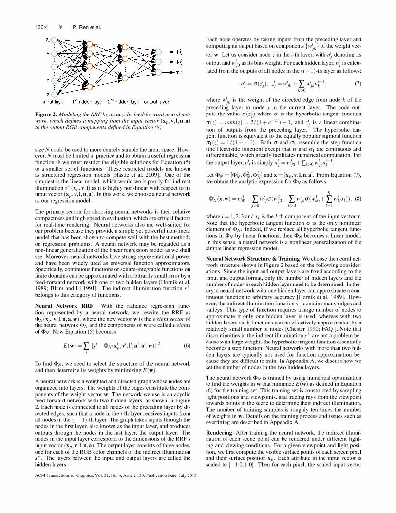
Figure 2: Modeling the RRF by an acyclic feed-forward neural net-work, which defines a mapping from the input vector (xp,v, l,n,a)to the output RGB components defined in Equation (8).

size N could be used to more densely sample the input space. How-ever, N must be limited in practice and to obtain a useful regressionfunction Φ we must restrict the eligible solutions for Equation (5)to a smaller set of functions. These restricted models are knownas structured regression models [Hastie et al. 2009]. One of thesimplest is the linear model, which would work poorly for indirectillumination s+(xp,v, l) as it is highly non-linear with respect to itsinput vector (xp,v, l,n,a). In this work, we choose a neural networkas our regression model.

The primary reason for choosing neural networks is their relativecompactness and high speed in evaluation, which are critical factorsfor real-time rendering. Neural networks also are well-suited forour problem because they provide a simple yet powerful non-linearmodel that has been shown to compete well with the best methodson regression problems. A neural network may be regarded as anon-linear generalization of the linear regression model as we shallsee. Moreover, neural networks have strong representational powerand have been widely used as universal function approximators.Specifically, continuous functions or square-integrable functions onfinite domains can be approximated with arbitrarily small error by afeed-forward network with one or two hidden layers [Hornik et al.1989; Blum and Li 1991]. The indirect illumination function s+belongs to this category of functions.

Neural Network RRF With the radiance regression func-tion represented by a neural network, we rewrite the RRF asΦN(xp,v, l,n,a,w), where the new vector w is the weight vector ofthe neural network ΦN and the components of w are called weightsof ΦN . Now Equation (5) becomes

E(w) = ∑i||yi−ΦN(xi

p,vi, li,ni,ai,w)||2. (6)

To find ΦN , we need to select the structure of the neural networkand then determine its weights by minimizing E(w).

A neural network is a weighted and directed graph whose nodes areorganized into layers. The weights of the edges constitute the com-ponents of the weight vector w. The network we use is an acyclicfeed-forward network with two hidden layers, as shown in Figure2. Each node is connected to all nodes of the preceding layer by di-rected edges, such that a node in the i-th layer receives inputs fromall nodes in the (i−1)-th layer. The graph takes inputs through thenodes in the first layer, also known as the input layer, and producesoutputs through the nodes in the last layer, the output layer. Thenodes in the input layer correspond to the dimensions of the RRF’sinput vector (xp,v, l,n,a). The output layer consists of three nodes,one for each of the RGB color channels of the indirect illuminations+. The layers between the input and output layers are called thehidden layers.

Each node operates by taking inputs from the preceding layer andcomputing an output based on components wi

jk of the weight vec-tor w. Let us consider node j in the i-th layer, with ni

j denoting itsoutput and wi

j0 as its bias weight. For each hidden layer, nij is calcu-

lated from the outputs of all nodes in the (i−1)-th layer as follows:

nij = σ(zi

j), zij = wi

j0 + ∑k>0

wijkni−1

k , (7)

where wijk is the weight of the directed edge from node k of the

preceding layer to node j in the current layer. The node out-puts the value σ(zi

j) where σ is the hyperbolic tangent functionσ(z) = tanh(z) = 2/(1 + e−2z)− 1, and zi

j is a linear combina-tion of outputs from the preceding layer. The hyperbolic tan-gent function is equivalent to the equally popular sigmoid functionσ1(z) = 1/(1+ e−z). Both σ and σ1 resemble the step function(the Heaviside function) except that σ and σ1 are continuous anddifferentiable, which greatly facilitates numerical computation. Forthe output layer, ni

j is simply nij = wi

j0 +∑k>0 wijkni−1

k .

Let ΦN = [Φ1N ,Φ

2N ,Φ

3N ] and x = [xp,v, l,n,a]. From Equation (7),

we obtain the analytic expression for ΦN as follows:

ΦiN(x,w) = w3

i0 + ∑j>0

w3i jσ(w2

j0 + ∑k>0

w2jkσ(w1

k0 +9

∑l=1

w1klxl)), (8)

where i = 1,2,3 and xl is the l-th component of the input vector x.Note that the hyperbolic tangent function σ is the only nonlinearelement of ΦN . Indeed, if we replace all hyperbolic tangent func-tions in ΦN by linear functions, then ΦN becomes a linear model.In this sense, a neural network is a nonlinear generalization of thesimple linear regression model.

Neural Network Structure & Training We choose the neural net-work structure shown in Figure 2 based on the following consider-ations. Since the input and output layers are fixed according to theinput and output format, only the number of hidden layers and thenumber of nodes in each hidden layer need to be determined. In the-ory, a neural network with one hidden layer can approximate a con-tinuous function to arbitrary accuracy [Hornik et al. 1989]. How-ever, the indirect illumination function s+ contains many ridges andvalleys. This type of function requires a large number of nodes toapproximate if only one hidden layer is used, whereas with twohidden layers such functions can be effectively approximated by arelatively small number of nodes [Chester 1990; FAQ ]. Note thatdiscontinuities in the indirect illumination s+ are not a problem be-cause with large weights the hyperbolic tangent function essentiallybecomes a step function. Neural networks with more than two hid-den layers are typically not used for function approximation be-cause they are difficult to train. In Appendix A, we discuss how weset the number of nodes in the two hidden layers.

The neural network ΦN is trained by using numerical optimizationto find the weights in w that minimize E(w) as defined in Equation(6) for the training set. This training set is constructed by samplinglight positions and viewpoints, and tracing rays from the viewpointtowards points in the scene to determine their indirect illumination.The number of training samples is roughly ten times the numberof weights in w. Details on the training process and issues such asoverfitting are described in Appendix A.

Rendering After training the neural network, the indirect illumi-nation of each scene point can be rendered under different light-ing and viewing conditions. For a given viewpoint and light posi-tion, we first compute the visible surface points of each screen pixeland their surface position xp. Each attribute in the input vector isscaled to [−1.0,1.0]. Then for each pixel, the scaled input vector

130:4 • P. Ren et al.


(a) (b)

(c) (d)

Figure 3: Comparison of RRFs with/without surface normal andSVBRDF attributes. (a) Ground truth by path tracing. (b) RRFswith augmented attributes, including both surface normal andSVBRDF parameters. (c) RRFs with basic attributes plus onlySVBRDF parameters. (d) RRFs with only basic attributes (no sur-face normal or SVBRDF parameters).

(xp,v, l,n,a) is input to the neural network ΦN to compute the indi-rect illumination value. These indirect illumination results are thenadded to those of direct illumination to generate the final rendering.

Run-time evaluation of ΦN is easy because both a(xp) and n(xp)can be made available in the graphics pipeline. As mentioned ear-lier, a(xp) is stored as a set of texture maps and is thus accessiblethrough texture mapping. n(xp) is also available because it is cal-culated in evaluating the direct illumination s0 in Equation (1). Bycontrast, other factors that affect indirect illumination, such as thedistance and angles of other scene points, are relatively unsuitablefor inclusion in the input vector. Not only are these quantities notreadily available in the graphics pipeline, but they would requirea substantial number of inputs to represent, which would signifi-cantly increase the number of neural network weights that need tobe learned. Each additional input adds n1 weights to the neural net-work, where n1 is the number of nodes in the first hidden layer.Since our design principle for the RRF is to make it compact andfast to evaluate, we limit the number of additional inputs and onlychoose quantities that are readily available.

Figure 3 displays rendering results of a simple scene consistingof two objects, a sphere and a box, each of which is modeledby an RRF. The ground truth image in (a) was rendered with thephysically-based offline path tracer [Lafortune and Willems 1993]used in generating the training data. Here the sphere is textured bya normal map and a spatially variant isotropic Ward BRDF [Ward1992], whose spatially variant parameter a(xp) is a 7D vector con-sisting of 3D diffuse and specular colors and 1D specular rough-ness. The same training data set is used to generate (b), (c) and(d). In comparison to RRFs with only basic attributes (d) or basicattributes plus only SVBRDF parameters (c), the inclusion of bothsurface properties among the augmented attributes leads to higherfidelity reproduction of surface details (b). Other frequently-usedparametric BRDF models such as the Cook-Torrance model, Blinn-Phong model, anisotropic Ward model, and Ashikhmin-Shirleymodel can also be effectively utilized in this manner.

Figure 4: Partitioning of input space for fitting of multiple RRFs.

4 Handling Scene Complexity

Input Space Partitioning So far, we have not considered complexscenes with many objects. In theory, such a scene could be approx-imated by a single RRF with a large number of nodes in the hiddenlayers. However, this significantly complicates RRF training, asthe number of weights to be learned increases quadratically withthe number of hidden-layer nodes. More importantly, a larger net-work leads to a much greater evaluation cost, which also increasesquadratically with the number of hidden-layer nodes. As a result,expanding the neural network quickly becomes infeasible for real-time rendering.

We address this issue by decomposing the space spanned by neu-ral network input vectors into multiple regions and fitting a separateRRF to the training data of each region. To partition the input space,we take advantage of the fact that the scene is already divided intodifferent 3D objects as part of the content creation process (typi-cally each object is topologically disconnected from other objectsin the scene). For each 3D object, we subdivide its input space usinga kd-tree, which is a binary tree suitable for recursive subdivision ofa high-dimensional space. With this partition, the computation ofthe indirect illumination value for an input only involves a kd-treesearch, which is extremely fast, and an evaluation of a small RRF.For each object, its input space is an n-dimensional box, and we de-note its kd-tree as Σ. Every non-leaf node ν in Σ is an n-dimensionalpoint, which implicitly generates a splitting hyperplane that dividesthe current-level box into two boxes at the next level of the kd-tree.Each non-leaf node is associated with one of the n dimensions xi,such that the splitting hyperplane is perpendicular to that dimen-sion’s axis. For simplicity we always split the current-level boxthrough the middle, generating two next-level boxes of equal size.The box to the left of the splitting hyperplane belongs to the leftsubtree of node ν , and the box to the right belongs to the right sub-tree. Finally, the leaf nodes of the kd-tree Σ hold boxes that are notsubdivided further.

Figure 4 illustrates the subdivision processing at a node ν , high-lighted in (a). We take the training samples within the n-dimensional box ω associated with the node ν and fit an RRF tothem. To reduce discontinuity across adjacent boxes, we includeadditional training samples from neighboring boxes by expandingthe box ω by 10% along each dimension as shown in (b). We couldfurther reduce discontinuities across the boundary of adjacent boxesby creating a small transition zone and linearly interpolating the ad-jacent RRFs. However, through experiments we found this to beunnecessary. Before training, we normalize the bounding box ofthe samples to a unit hypercube as shown in (c-d). We stop sub-dividing the node ν when both training and prediction errors areless than 5% (relative error). Here the prediction error is measuredby evaluating the RRF against a test set removed from the pool ofall training samples. In our experiments, we remove 30% of the



training samples for testing.

If further subdivision of the node ν is required, we need to choosean axis xi for splitting ν . The best splitting axis is the one thatgenerates the smallest training and prediction errors on the childnodes of ν . A brute-force way to find this axis is to try every axisand carry out the RRF fitting and testing process on the resultingchild nodes. Alternatively, we could randomly select a splittingaxis, which results in roughly 10% higher RRF fitting and testingerrors in our experiments.1 For the results reported in this paper,we use the brute-force method to identify the splitting axis.

The use of augmented attributes instead of only basic attributes in-creases the apparent dimensionality of the input space, which couldmake the subdivision process less efficient by creating a larger num-ber of insignificant cells. However, we note that though s+a appearsto be a higher dimensional function than s+, the intrinsic dimen-sionality of s+a is no greater than s+ because both a and n are notindependent variables but rather functions of xp, which is alreadyan attribute in the input vector of s+. The function s+a is simply theoriginal function s+ embedded in a higher dimensional space. Sinceour kd-tree subdivision criteria is completely driven by fitting andprediction errors, a cell will be created only when necessary (i.e.,when the errors are too high) and this fact remains true no matterwhich space s+ is embedded. This error-driven subdivision criteriaensures that no unnecessary cells are created.

A benefit of using kd-trees over a quadtree/octree-like partitioningstructure is that node splits are not jointly performed over all di-mensions, which may lead to an overabundance of nodes in thehigh-dimensional space and hence many more RRFs than needed.

Lighting Complexity Our discussion so far focuses on the case ofa single point light source. It is straightforward to handle the gen-eral case of any finite number of local lights of any colors. Moreimportantly, this can be done without recomputing the RRF ΦN .Suppose there are K light sources with the k-th light located at po-sition lk. Since ΦN is computed for a unit light source and lighttransport is linear with respect to light intensities, the indirect illu-mination s+ may be written as

s+(xp,v, l1, ..., lK) =k=K

∑k=1

ckΦN(xp,v, lk,n,a,w), (9)

where ck is the color of the k-th light. This equation implies that thelight positions and colors are all variables that are free to change in-dependently under user control. Since each term in the sum is eval-uated by the same RRF ΦN , no additional training or storage costis needed for multiple point lights. At run time, the main cost is theevaluation of ΦN for multiple light positions and the computationof direct illumination for each of the lights.

Note that the linearity of light transport allows us to handle any fi-nite number of local lights of any colors by using the same RRFΦN . Without this property, we would have to simultaneously in-clude the positions and colors of all lights as input variables of ΦN ,resulting in a neural network that is prohibitively expensive to trainand store.

5 Implementation and Results

We implemented the proposed partitioning and training algorithmon a PC cluster with 200 nodes, each of which is configured with

1Note that these errors are only used for guiding the subdivision of non-leaf nodes; the final fitting and testing errors on the leaf nodes are deter-mined by the same stopping criteria no matter how splitting axes are chosen.

Scene Vertex Num. Sample Num. Partition Num. Sampling Time Training TimeCornellBox 29K 10M 6.5K 0.25h 0.75hPlant 194K 110M 75.5K 3h 7.5hKitchen 122K 60M 32.5K 12h 1.5hSponza 31K 50M 33.0K 2.5h 1.2hBedroom 194K 190M 127.4K 75h 10h

Table 1: Performance data on RRF training.

Scene RRF Size FPS Dir. Shading Tree Trav. RRF Eval.CornellBox 5.64MB 61.9fps 5.33ms 2.39ms 8.43msPlant 66.77MB 32.6fps 5.10ms 2.52ms 23.05msKitchen 33.12MB 36.5fps 15.341ms 2.37ms 9.62msSponza 24.81MB 60.8fps 6.75ms 2.16ms 7.54msBedroom 109.09MB 69.1fps 2.61ms 2.44ms 9.40ms

Table 2: Performance data on RRF-based rendering. Dir. shadingdenotes the computation time for direct shading. Tree Trav. is thecomputation time for partition tree traversal, and RRF Eval. repre-sents the time for RRF evaluation.

two Quadcore Intel Xeon L5420 2.50G CPUs and 16GB of mem-ory. The indirect illumination values for the training set are com-puted using the Mitsuba renderer [Jakob 2010] on the same clus-ter. The real-time rendering algorithm is implemented on an nVidiaGeForce GTX 680 with 2GB of video memory. The direct il-lumination component is calculated with a programmable render-ing pipeline using variance shadow maps [Donnelly and Lauritzen2006].

At run time, we use CUDA to compute the indirect illuminationvalue for each screen pixel as follows. The input vectors of all pix-els are stored in a matrix M that is converted from the G-buffersof the deferred shading pipeline, one input vector per matrix col-umn. Since a kd-tree is built for each 3D object, we also store anobject ID with each input vector so that it is easy to locate the cor-responding kd-tree. In the CUDA kernel for kd-tree traversal, eachthread reads an input vector x from the matrix M, locates a kd-tree,and traverses down the kd-tree to reach a leaf node, where it picksup the ID of the neural network ΦN for the partition containing x.Then in the neural network CUDA kernel, each thread feeds the in-put vector x to the neural network ΦN and evaluates the color valueof the pixel according to Equation (8).

We tested our method on a variety of scenes that exhibit differ-ent light transport effects. The Cornell Box scene (Figure 9 a-b)includes rich interreflection effects between the diffuse and spec-ular surfaces, such as color bleeding and caustics. In the Plantscene (Figure 9 c-d), the fine geometry of the plant model resultsin complex occlusions and visibility change. The Kitchen scene(Figure 10) is used to illustrate view-dependent indirect illumina-tion effects caused by strong interreflections between specular sur-faces. We also tested the scalability of our method on two complexscenes. The Sponza scene (Figure 11) consists of diffuse surfaceswith complex geometry. In the Bedroom scene (Figure 12), objectswith different shapes and material properties are placed togetherand they present rich and complicated shading variations under dif-ferent lighting and viewing conditions.

Table 1 lists for each scene the number of vertices and detailedtraining performance data, including training data sizes and tim-ings for training sample generation and the training process.The

Scene Mean error Random training set Random weight init.CornellBox 0.029 0.00021 0.00018Plant 0.066 0.00014 0.00014Kitchen 0.056 0.00008 0.00032

Table 3: Rendering accuracy of three scenes, and robustness withrespect to different choices of training data set and different initialneural network weight values.

130:6 • P. Ren et al.


(a) (b) (c)

(d) (e) (f)

(g) (h) (i)

Figure 5: Comparison of results rendered by our method and thoseof path tracing. Only indirect illumination results are shown. Left:Path tracing results. Middle: Our rendering results. Right: Differ-ence between the two results.

run-time rendering performance for each scene is reported in Ta-ble 2. The relatively long RRF evaluation time for the Plant sceneis due to its intricate geometry, which leads to many neighboringpoints belonging to different partitions and hence low data coher-ence. The image resolution for all the renderings is 512×512.

Method Validation We validate our RRF training and renderingmethod with the Cornell Box, Plant and Kitchen scenes. To eval-uate accuracy, we compare the images rendered by our method toground truth images generated by Mitsuba path tracing with eachpixel rendered using 16384 rays for the Cornell Box scene, 4096rays for the Plant scene, and 32768 rays for the Kitchen scene. Inthis experiment, we rendered 400 images of 512× 512 resolutionwith pairings between 20 randomly selected view positions and 20random light positions, none of which were used in the training set.The rendering error E was computed as the root-mean-square errorof the 400 image pairs. The first column of Table 3 shows the meanerrors for three scenes. Figure 5 shows our results, the ground truthimages, and the differences between them. It is seen that the RRFsaccurately predict the indirect illumination values of surface pointsunder novel lighting, and they generate results that are visually sim-ilar to the ground truth. Note that the errors in textured regions aremainly due to the different texture filters used in Mitsuba and ourRRF rendering, while the errors along object boundaries are causedby the single sample ray for each pixel used in our RRF rendering.

To test the robustness of our training method with different trainingsets, we trained the RRFs with 70% of the samples randomly se-lected from the full training set and used the RRFs to render the 400images mentioned above. This was done a total of ten times withdifferent sets of training samples, and the rendering results wereeach compared to ground truth. We found that for the ten resultingneural networks, their mean rendering errors are approximately thesame as that of the original RRF fitting, and the standard deviationof the errors is very small. We report the standard deviation of theerrors for the three scenes in the second column of Table 3. We alsoexamined in a similar manner the robustness of our training methodfor different initial weight values. In each experiment, we use thesame training data but with different initial weight values within

(a) (b)0.625M (c)2.5M

(d)10M (e)40M (f)Traced

Figure 6: Accuracy of RRFs generated from training sets of dif-ferent sizes. (a) Rendering errors of RRFs computed from differ-ent sizes of training data. (b)-(e) Rendering results of the differentRRFs. (f) Ground truth image.

[−1.0,1.0]. The standard deviations of the rendering errors overthe ten sets of RRF rendering results for the three scenes are listedin the third column of Table 3. These experiments indicate thatour training method is stable and robust with respect to differentchoices of initial weight values and different selections of trainingdata. The different rendering results for a given input vector alsovisually appear similar.

The accuracy of RRFs is mainly determined by the size and ac-curacy of the training set. Figure 6(a) plots the rendering errorsof RRFs computed from different amounts of training data for theCornell Box scene. Figure 6(b)-(f) illustrates the rendering resultsof the RRFs and the ground truth image generated by path tracing.Although the RRFs trained from relatively little data can well re-construct the low-frequency shading variations over the surface, therich shading details are lost. As the size of training data increases,the accuracy of RRFs improves quickly and become stable after thenumber of training samples reaches 10M (i.e. the size used in ourimplementation). Beyond that, the accuracy and rendering qualityof RRFs improves slowly as the size of training data increases. Fig-ure 7(a) plots the rendering errors of RRFs computed from trainingsets generated with different levels of accuracy also for the CornellBox scene. The number of training samples is 10M in this experi-ment while each training set is generated by path tracing with differ-ent numbers of rays. Figure 7(b)-(f) shows the rendering results ofRRFs and the ground truth image, which was rendered with 16384rays. When decreasing the number of rays used in training set gen-eration from 4096 to 256, the noise in the sampling data becomeslarger, which leads to larger error in RRF rendering and blockingartifacts in regions with smooth shading. On the other hand, theaccuracy of RRFs is stable as the number of rays grows from 4096to 16384, since the accuracy of training samples improves little be-yond using 4096 rays in path tracing. Based on this, our imple-mentation for rest of the paper uses 4096 rays to generate the RRFtraining data.

Rendering results Figure 9(a-b) displays rendering results of theCornell Box scene under different lighting and viewing conditions.In this scene, the left/right wall, ceiling and floor are diffuse sur-faces, and all the remaining objects are glossy. The color bleedingbetween the side walls and ceiling is well reproduced. The causticscaused by the ring and statue are convincingly generated. Figure9(c-d) shows rendering results of the Plant scene. The multi-bounceinterreflections on the desktop and the plant leaves closely matchground truth.



(a) (b)256 (c)1024

(d)4096 (e)16384 (f)Traced

Figure 7: Accuracy of RRFs generated from training sets renderedwith different numbers of rays. (a) Rendering errors of RRFs withrespect to the number of rays used in training data generation. (b)-(e) Rendering results of the different RRFs. (f) Ground truth image.

In Figure 10, rendering results are displayed for the Kitchen scene,where the multi-bounce interreflections between the glossy sur-faces generate strong indirect illumination effects. With differentviewpoints, the changing reflections of the fruits and bottles on theback wall and desktop are well reproduced. For comparison, wealso show the scene rendered with only direct illumination in Fig-ure 10(d).

Figure 11 shows renderings of the Sponza scene. The shading vari-ations caused by multi-bounce interreflections are accurately gen-erated, including interreflections with three or more bounces in theroof of the cloister arcade as shown in (a), and shadows cast byindirect lighting in (c).

The Bedroom scene, which exhibits complex indirect illuminationeffects, is rendered in Figure 12. Rendering all complex lightingeffects in the scene is a challenging task even for offline global illu-mination algorithms. Our method reproduces all the lighting effectsin real time with only 109.09 MB of RRF data. Both the smooth in-direct illumination from diffuse surfaces and the detailed reflectionsfrom glossy objects are well rendered.

The accompanying video provides real-time rendering results of allthe scenes with dynamic viewpoint and lighting. The video alsoincludes real-time rendering with multiple dynamic local lights ofchanging colors, as well as examples of real-time material editingas discussed below.

Material Editing The RRF provides a flexible technique for real-time material editing, which benefits greatly from the RRF’s abilityto capture advanced visual effects such as changing caustics (Fig-ure 8 a-b) and high-frequency glossy interreflections (Figure 8 c-d).For further details, please refer to Appendix B.

6 Discussion

Although our approach is also based on precomputation for ren-dering global illumination effects in real time, it is conceptuallydifferent from PRT methods and has very different properties. AllPRT methods model the global illumination of each surface pointas a linear function between incoming and outgoing radiance. Todeal with 6D indirect global illumination (with respect to surfaceposition, viewing direction, and distant lighting direction), thesemethods densely sample 2D object surfaces and encode the 4D lighttransport of each surface point with a linear or non-linear basis.This separate representation takes advantage of the non-linear co-

(a) (b)

(c) (d)

Figure 8: Extension of RRFs to real-time material editing. (a)(b)Changing the specular color of the statue and the glossiness of thering. (c)(d) Editing the diffuse color of the fruits and the glossinessof the back wall.

herence in the 6D indirect global illumination in a limited way. Inparticular, the scene must be densely tessellated in order to modelhigh-frequency lighting effects on the surface. Although the datasize can be reduced by different data compression schemes such asCPCA and clustered tensor approximation, these piecewise linearor multi-linear compression schemes prevent full exploitation ofthe non-linear coherence in the data. A large amount of data andcomputation is needed for rendering high-frequency lighting ef-fects, such as caustics, sharp indirect shadows, and high-frequencyglossy interreflections. To our knowledge, no existing PRT methodcan render all of these effects in real time for local light sources.

By contrast, our method directly approximates the 6D indirectglobal illumination and can effectively take advantage of the non-linear coherence in all six dimensions simultaneously. Moreover,the precomputed neural networks have analytic forms and do notrequire dense surface meshing to capture high-frequency lightingeffects. For the Cornell Box scene which exhibits caustics and com-plex interreflections of multiple glossy objects, our method needsonly 5.6 MB of data for rendering the scene at 60 FPS. For compar-ison, Green et al. [2006] modeled incident lighting with a mixtureof spherical Gaussians, which requires about 25 MB of data to ren-der one single homogeneous glossy object. With Kristensen et al.’sapproach [2005], a single glossy bunny model can be rendered with17 MB of precomputed and compressed data. The direct-to-indirecttransfer methods presented by Kontkanen et al. [2006] sample the4D transport matrix of direct light to indirect light at each surfacepoint and encode the transport matrix using a wavelet basis. It re-quires 23 MB of data to render the low-resolution indirect lightingof a small scene with two glossy objects. Because of the complexityof the compression scheme (4D wavelet basis), the rendering framerate is low (about 10 FPS).

While the performance of our method is independent of the den-sity of mesh tessellations (i.e. the number of vertices), it is af-fected by the scale and geometric configuration of the scene. As thescale of the scene becomes larger, the coherence of indirect light-ing among the different regions of the scene decreases accordingly,

130:8 • P. Ren et al.


which leads to more partitions and RRFs needed for rendering. Forthe Sponza scene, our method uses 24.81 MB of data for renderingits lighting effects throughout the scene. The indirect shadowing ef-fects in the scene are effectively rendered. For reference, Kristensenet al.’s solution used about 17 MB of data for modeling the diffuseinterreflections in the same scene. Since the shading effects aresampled over the sparse mesh vertices, the detailed indirect shad-owing effects between vertices are lost. The meshless approach ofLehtinen et al. [2008] needs 77.4 MB data to achieve a renderingquality similar to our method for this scene. For scenes with sharpindirect shadowing effects that are caused by complicated geome-try configurations (e.g. the Bedroom scene and the Plant scene),our method also needs more RRFs for rendering. Note that thesescenes are also challenging for previous PRT methods.

In this work we have considered lighting environments composedof point light sources, but RRFs can be utilized with other types oflight sources as well. For example, directional lights can be han-dled by training RRFs of the form ΦN(xp,v,d,n,a,w), where d isthe light direction. However, environment lighting must be han-dled carefully because allowing unlimited change of every pixel inthe environment map could lead to an explosion in the degrees offreedom of the input vector, and thus make the training of RRFsimpractical. If only rotation of the environment light is needed, thismay be achieved by training RRFs of the form ΦN(xp,v,r,n,a,w),where r is the rotation vector of the environment light. For moregeneral changes of environment light, we can adjust low-frequencylighting as in PRT by projecting the light onto a spherical harmonicsbasis and selecting the first few terms of the basis expansion as RRFinputs. One RRF can then be trained for each selected basis func-tion, and the RRFs so trained can be combined as in Equation (9).

There are other ways to parameterize the input variables xp and vof the RRF ΦN(xp,v, l,n,a,w). If there is no participating mediain the scene, then we are only interested in points xp on surfaces,which can be parameterized by two variables up, vp. This wouldreduce the degrees of freedom and make RRF training easier. Inthis work, we choose to directly work with 3D points xp becausein practice graphics objects often come in different formats and itis not always easy to parameterize them. We also want to leave theRRF in a general form suitable for scenes with participating media.The same consideration applies to the viewing vector v.

Our current system takes a long time for preprocessing. We madeno effort to optimize this lengthy preprocessing stage because ourfocus was on achieving real-time rendering without sacrificing anyglobal illumination effects. In the future, much work can be doneto reduce the precomputation time. The precomputation includestwo parts: sampling the training data and neural network training.The long computation time for sampling is due to the brute-forcepath tracing algorithm used in our current implementation. Thistime could be greatly reduced by using faster global illuminationalgorithms (e.g. photon mapping). The neural network trainingcode is not optimized and takes 1∼10 hours to generate the neuralnetworks of each example in the paper. This could be acceleratedby 10X∼30X on the GPU.

The main limitation of the RRF is that the dimensionality of the in-put vector should not be too high. With a large number of indepen-dent variables in the input vector, training the neural network be-comes impractical in terms of both the training time and the amountof training data needed. Our work shows that dynamic viewpointand local lights can be handled well. However, introducing addi-tional dynamic elements such an animated objects into the scenerequires care. Dynamic elements should be added in a manner thatthe degrees of freedom in the scene remain manageable.

Another limitation of the RRF is that it provides a good approxima-tion only of the indirect illumination near sampled viewing direc-

tions and light positions. In other words, the RRF works well wheninterpolating between samples but poorly when extrapolating froma neighboring sample.

7 Conclusion

We described the radiance regression function as a nonlinear modelof indirect illumination for dynamic viewing and lighting condi-tions. Our experiments show that convincing rendering includingchallenging visual effects such as high-frequency glossy interreflec-tions can be achieved with a relatively compact RRF model, whichindicates that significant non-linear coherence exists in the indirectillumination data. This coherence can be effectively exploited byreal-time rendering methods that are based on precomputed globalillumination. Our RRF representation is run-time local in the sensethat the run-time evaluation of the RRFs of each 3D object doesnot involve any other objects in the scene. Thus the rendering canremain real-time even for a large scene with many objects, becauseall objects are rendered in parallel in screen space.

We plan to investigate a couple of directions for further work. Wecurrently only work with opaque objects and assume there is no par-ticipating media. Future directions may include handling of translu-cent objects and participating media. We are also interested in waysto reduce the training time. Finally, we intend to investigate meth-ods for efficiently handling dynamic scenes. Though scaling upfrom the few degrees of freedom in this paper to the many degreesof freedom of less constrained scene configurations presents a sig-nificant challenge, this problem could potentially be simplified byadapting the set of attributes for an object/region to account only foranimated objects that can have a discernible effect on its shading.

Acknowledgements

The authors thank Zhuowen Tu and Frank Seide for helpful dis-cussions on nonlinear regression techniques and neural networktraining. The authors also thank the anonymous reviewers for theirhelpful suggestions and comments. The scene in Figure 10 wasprovided by Tomas Davidovic, and the scene in Figure 12 was geo-metrically modeled by David Vacek and designed by Shuitan Yan.

References

BEALE, M. H., HAGAN, M. T., AND DEMUTH, H. B. 2012.Neural Network Toolbox user’s guide.

BLUM, E., AND LI, L. 1991. Approximation theory and feedfor-ward networks. Neural Networks 4, 4, 511–515.

CHESTER, D. 1990. Why two hidden layers are better than one. InInt. Joint Conf. on Neural Networks (IJCNN), 265–268.

COHEN, M. F., WALLACE, J., AND HANRAHAN, P. 1993. Radios-ity and realistic image synthesis. Academic Press Professional,Inc., San Diego, CA, USA.

CRASSIN, C., NEYRET, F., SAINZ, M., GREEN, S., AND EISE-MANN, E. 2011. Interactive indirect illumination using voxelcone tracing. Computer Graphics Forum 30, 7.

DACHSBACHER, C., AND STAMMINGER, M. 2006. Splatting in-direct illumination. In I3D, 93–100.

DACHSBACHER, C., STAMMINGER, M., DRETTAKIS, G., ANDDURAND, F. 2007. Implicit visibility and antiradiance for inter-active global illumination. ACM Trans. Graph. 26.

DACHSBACHER, C. 2011. Analyzing visibility configurations.IEEE Trans. Vis. Comput. Graph. 17, 4, 475–486.



(a) (b) (c) (d)

Figure 9: Rendering results using RRFs. (a)(b) Cornell Box scene. (c)(d) Plant scene.

(a) (b) (c) (d)

Figure 10: Kitchen scene with strong glossy interreflections. (c)(d) Comparison between global illumination and direct illumination results.

(a) (b) (c) (d)

Figure 11: Sponza scene with complex geometry. (a) Three or more light bounces are needed to reach the roof of the cloister arcade. (c)(d)Comparison between global illumination and direct illumination results.

(a) (b) (c) (d)

Indirect shadow

Figure 12: Bedroom scene with complex geometry and material variations. (c) Zoomed view of the indirect shadow highlighted in (b). (d)Ground truth of the indirect shadow rendered by path tracing.

130:10 • P. Ren et al.


DONG, Z., KAUTZ, J., THEOBALT, C., AND SEIDEL, H.-P. 2007.Interactive global illumination using implicit visibility. In PacificConference on Computer Graphics and Applications, 77–86.

DONIKIAN, M., WALTER, B., BALA, K., FERNANDEZ, S., ANDGREENBERG, D. P. 2006. Accurate direct illumination usingiterative adaptive sampling. IEEE TVCG 12 (May), 353–364.

DONNELLY, W., AND LAURITZEN, A. 2006. Variance shadowmaps. In I3D, 161–165.

FAQ. How many hidden layers should I use? Neural Net-work FAQ, Usenet newsgroup comp.ai.neural-nets, ftp://ftp.sas.com/pub/neural/FAQ3.html#A_hl.

GREEN, P., KAUTZ, J., MATUSIK, W., AND DURAND, F. 2006.View-dependent precomputed light transport using nonlineargaussian function approximations. In I3D, 7–14.

GRZESZCZUK, R., TERZOPOULOS, D., AND HINTON, G. 1998.Neuroanimator: fast neural network emulation and control ofphysics-based models. In Proc. SIGGRAPH ’98, 9–20.

HAGAN, M., AND MENHAJ, M. 1994. Training feedforward net-works with the marquardt algorithm. Neural Networks, IEEETransactions on 5, 6, 989 –993.

HASTIE, T., TIBSHIRANI, R., AND FRIEDMAN, J. 2009. TheElements of Statistical Learning: Data Mining, Inference, andPrediction, 2 ed. Springer.

HASAN, M., PELLACINI, F., AND BALA, K. 2006. Direct-to-indirect transfer for cinematic relighting. ACM Trans. Graph.25, 1089–1097.

HERTZMANN, A. 2003. Machine learning for computer graphics:A manifesto and tutorial. In Pacific Conference on ComputerGraphics and Applications, 22–36.

HINTON, G. E. 1989. Connectionist learning procedures. ArtificialIntelligence 40, 1-3, 185–234.

HORNIK, K., STINCHCOMBE, M., AND WHITE, H. 1989. Multi-layer feedforward networks are universal approximators. NeuralNetworks 2, 5 (July), 359–366.

JAKOB, W., 2010. Mitsuba renderer. Department of ComputerScience, Cornell University. (http://www.mitsuba-renderer.org).

KAPLANYAN, A., AND DACHSBACHER, C. 2010. Cascaded lightpropagation volumes for real-time indirect illumination. In I3D,99–107.

KELLER, A. 1997. Instant radiosity. In SIGGRAPH ’97, 49–56.

KONTKANEN, J., TURQUIN, E., HOLZSCHUCH, N., AND SIL-LION, F. X. 2006. Wavelet radiance transport for interactiveindirect lighting. In Rendering Techniques ’06, 161–171.

KRISTENSEN, A. W., AKENINE-MOLLER, T., AND JENSEN,H. W. 2005. Precomputed local radiance transfer for real-timelighting design. ACM Trans. Graph. 24, 1208–1215.

LAFORTUNE, E. P., AND WILLEMS, Y. D. 1993. Bi-directionalpath tracing. In Proc. Compugraphics ’93, 145–153.

LEHTINEN, J., ZWICKER, M., TURQUIN, E., KONTKANEN, J.,DURAND, F., SILLION, F. X., AND AILA, T. 2008. A mesh-less hierarchical representation for light transport. ACM Trans.Graph. 27, 37:1–37:9.

LIU, X., SLOAN, P.-P., SHUM, H.-Y., AND SNYDER, J. 2004.All-frequency precomputed radiance transfer for glossy objects.In Rendering Techniques ’04, 337–344.

MCGUIRE, M., AND LUEBKE, D. 2009. Hardware-acceleratedglobal illumination by image space photon mapping. In HighPerformance Graphics.

MCKAY, M. D., BECKMAN, R. J., AND CONOVER, W. J. 2000.A comparison of three methods for selecting values of input vari-ables in the analysis of output from a computer code. Techno-metrics 42, 1 (Feb.), 55–61.

MEYER, M., AND ANDERSON, J. 2007. Key point subspace ac-celeration and soft caching. ACM Trans. Graph. 26, 3.

NG, R., RAMAMOORTHI, R., AND HANRAHAN, P. 2004. Tripleproduct wavelet integrals for all-frequency relighting. ACMTrans. Graph. 23, 477–487.

NICHOLS, G., AND WYMAN, C. 2010. Interactive indirect illumi-nation using adaptive multiresolution splatting. IEEE TVCG 16,5, 729–741.

NOWROUZEZAHRAI, D., KALOGERAKIS, E., AND FIUME, E.2009. Shadowing dynamic scenes with arbitrary brdfs. Com-put. Graph. Forum: Eurographics Conf. 28, 249–258.

PARKER, S. G., BIGLER, J., DIETRICH, A., FRIEDRICH, H.,HOBEROCK, J., LUEBKE, D., MCALLISTER, D., MCGUIRE,M., MORLEY, K., ROBISON, A., AND STICH, M. 2010. Optix:A general purpose ray tracing engine. ACM Trans. Graph. 29.

RAMAMOORTHI, R. 2009. Precomputation-based rendering.Found. Trends. Comput. Graph. Vis. 3 (April), 281–369.

RITSCHEL, T., GROSCH, T., KIM, M. H., SEIDEL, H.-P.,DACHSBACHER, C., AND KAUTZ, J. 2008. Imperfect shadowmaps for efficient computation of indirect illumination. ACMTrans. Graph. 27, 129:1–129:8.

RITSCHEL, T., DACHSBACHER, C., GROSCH, T., AND KAUTZ,J. 2012. The state of the art in interactive global illumination.Computer Graphics Forum 31, 1, 160–188.

SLOAN, P.-P., KAUTZ, J., AND SNYDER, J. 2002. Precom-puted radiance transfer for real-time rendering in dynamic, low-frequency lighting environments. ACM Trans. Graph. 21.

SLOAN, P.-P., HALL, J., HART, J., AND SNYDER, J. 2003. Clus-tered principal components for precomputed radiance transfer.ACM Trans. Graph. 22, 3 (July), 382–391.

THIEDEMANN, S., HENRICH, N., GROSCH, T., AND MULLER,S. 2011. Voxel-based global illumination. In I3D, 103–110.

TSAI, Y.-T., AND SHIH, Z.-C. 2006. All-frequency precomputedradiance transfer using spherical radial basis functions and clus-tered tensor approximation. ACM Trans. Graph. 25, 3, 967–976.

WALD, I., MARK, W. R., GUENTHER, J., BOULOS, S., IZE, T.,HUNT, W., PARKER, S. G., AND SHIRLEY, P. 2009. Stateof the art in ray tracing animated scenes. Computer GraphicsForum 28, 6, 1691–1722.

WANG, R., TRAN, J., AND LUEBKE, D. 2006. All-frequencyrelighting of glossy objects. ACM Trans. Graph. 25, 2, 293–318.

WANG, R., ZHU, J., AND HUMPHREYS, G. 2007. Precomputedradiance transfer for real-time indirect lighting using a spectralmesh basis. In Rendering Techniques ’07, 13–21.

WANG, R., WANG, R., ZHOU, K., PAN, M., AND BAO, H. 2009.An efficient gpu-based approach for interactive global illumina-tion. ACM Trans. Graph. 28 (July), 91:1–91:8.

WARD, G. J. 1992. Measuring and modeling anisotropic reflection.In Proc. SIGGRAPH ’92, 265–272.



ftp://ftp.sas.com/pub/neural/FAQ3.html#A_hl

ftp://ftp.sas.com/pub/neural/FAQ3.html#A_hl

Appendix A: Neural Network DetailsThe neural networks used in this work contain two hidden layers.To determine the numbers of nodes in these hidden layers, we ex-perimented with different node arrangements for the scene in Fig-ure 3. As shown in Figure 13, increases to the number of nodesin each layer lead to reductions in fitting error. Meanwhile, thenumber of weights also increases, which necessitates greater com-putation for neural network training and evaluation. In our currentimplementation, we use 20 nodes in the first hidden layer and 10nodes in the second hidden layer, which provides a good balancebetween approximation capability and computational efficiency.

To train the neural network, a set of training data must first be ob-tained. Given a scene with a predefined range of light source po-sitions and viewpoints, we generate the training set by a Latin hy-percube sampling scheme [McKay et al. 2000] and compute theindirect illumination values of all examples by path tracing [Lafor-tune and Willems 1993]. Specifically, we uniformly subdivide thelight range into Nl strata and randomly sample the light position ineach stratum. We then sample Nv viewpoint positions in a similarmanner. For each combination of light position l and viewpoint, werandomly shoot Nr rays from the viewpoint and trace each ray v tothe first intersection point x in the scene. We then record the sur-face point position xp and compute its indirect illumination valuevia path tracing. Through this process we generate Nl×Nv×Nr ex-amples that form the training set. The total number of samples is setto approximately ten times the number of neural network weights[Grzeszczuk et al. 1998]. The values of Nv, Nl and Nr are then cho-sen by the user based on scene complexity. For the scene shown inFigure 5(b), we set Nv = 200, Nl = 200, and Nr = 6000. Instead ofdirectly sampling points on a surface, our method samples intersec-tions on the surface of viewing rays, which avoids visibility testsand ensures that the visible surface is well sampled. We note thatsince some rays may not intersect points in the scene, the value ofNr may need to be increased to generate the targeted number of ex-amples. Other sampling techniques may alternatively be used herefor training set generation.

Having determined the structure of the neural network ΦN and thetraining set, we now train ΦN(xp,v, l,n,a,w) by solving for all theweights in w. This is done by applying the Levenberg-Marquardt(LM) algorithm as in [Hagan and Menhaj 1994] to minimize E(w)in Equation 6. For the small-scale neural networks used in our sys-tem, the LM algorithm demonstrates better performance than othergradient-based and conjugate methods [Hagan and Menhaj 1994].We follow the implementation in [Beale et al. 2012] to first com-pute the range of each element in both the input and output vectors,and scale each element to [−1.0,1.0] so that they are treated equallyin training. The scale factor of each attribute is saved for run-timecomputation. After the weight vector w is initialized with randomvalues in [−1.0,1.0], we then iteratively update w:

wn+1 = wn +(H +λdiag[H])−1g, (10)

where wn+1 and wn are the weight vectors in the current and pre-vious iterations. H is the Hessian matrix of E(w) with respect tow, which can be efficiently computed from the Jacobian matrix J ofE(w) as H = JT J. λ is a constant for controlling the step length andis automatically determined by the algorithm. g denotes the gradi-ent of the current error function E(wn) with respect to the weights,and is calculated as g= JT E(wn). In each iteration, we compute theJacobian matrix of E(wn) with a standard back-propagation scheme[Hinton 1989]. We repeat this process until the error E(w) dropsbelow a user-defined threshold (0.05 in our implementation).

We tried both batch training and online training [Hastie et al. 2009]for our task. In batch training we minimize E(w) with all trainingdata, while in online training we divide the training data into sub-groups and progressively update the weight vector by minimizing

Figure 13: Number of hidden-layer nodes vs. fitting error.

E(w) with a subgroup. For our application, we have found batchtraining to always outperform online training, and thus it is used inour implementation.

Overfitting is an important and well-studied issue in regression. Aneural network with too many free parameters will overfit the data.To avoid this we make sure that we have sufficient training data asin [Grzeszczuk et al. 1998], i.e., 8∼ 10 times the number of neuralnetwork weights. Another important technique is cross-validation:we use 70% of the training data for neural network training, and re-serve the remaining 30% to validate the training result [Beale et al.2012]. Finally, there is yet another technique called weight decay (aform of regularization) [Hastie et al. 2009]. We have implementedthis technique in our system as well but found little further improve-ment. In Section 6 we reported that our regression system is robustwith respect to different choices of training sets and initial weightvalues. This is another sign indicating that overfitting is under con-trol in our system.

Appendix B: Material EditingThe RRF provides a flexible technique for editing material proper-ties of selected objects in the scene, with the ability to visualize edit-ing results in real-time with full global illumination effects. Visualeffects that are usually challenging to capture with existing meth-ods, such as changing caustics and multiple-bounce high-frequencyglossy interreflection, can be well reproduced with RRFs. Depend-ing on the nature of the editing task, we can choose to fix either thelighting or the viewpoint, and replace the corresponding RRF inputvariables by the BRDF parameters of the selected objects. Fig-ure 8(a-b) shows the editing of the specular roughness of the ringand the specular color of the gargoyle in the Cornell Box scene. Inthis example, we are particularly interested in how the caustics gen-erated by the ring change as the specular roughness and the lightingchange. Thus we choose to fix the viewpoint and replace the view-ing direction variables of the RRFs by new variables representingthe specular roughness of the ring and the specular color of the gar-goyle. A training set is generated based on the new input vector, andthe RRFs are obtained by regression with respect to the new trainingdata. The resulting RRFs support real-time editing of these mate-rial properties since they are now the input variables of the RRFs,as demonstrated in the companion video. Figure 8(c-d) shows theediting of fruit colors and the specular roughness of the back wallin the Kitchen scene. In this example, we choose to focus on themultiple-bounce high-frequency glossy interreflection on the backwall as seen from different viewpoints. Again, we can easily ac-commodate this choice by fixing the light position and leaving theviewing direction as an input variable of the RRFs, while support-ing material editing by using the color of the fruits and the specularroughness of the back wall as RRF input variables when generatingtraining data and performing RRF regression. Note that multiple-bounce high-frequency glossy interreflection is very difficult to cap-ture with most existing methods because these methods commonlyassume that multiple-bounce interreflection is low-frequency.

130:12 • P. Ren et al.


Documents

Global illumination with radiance regression functions