Global Illumination Compendium 1

Global Illumination Compendium

September 29, 2003

Philip Dutréphil@cs.kuleuven.ac.be

Computer Graphics, Department of Computer ScienceKatholieke Universiteit Leuven

http://www.cs.kuleuven.ac.be/~phil/GI/

This collection of formulas and equations is supposed to be useful for anyone who is active in the field of global illu-mination in computer graphics. I started this document as a helpful tool to my own research, since I was growing tiredof having to look up equations and formulas in various books and papers. As a consequence, many concepts which are‘trivial’ to me are not in this Global Illumination Compendium, unless someone specifically asked for them. There-fore, any further input and suggestions for more useful content are strongly appreciated.

If possible, adequate references are given to look up some of the equations in more detail, or to look up the deriva-tions. Also, an attempt has been made to mention the paper in which a particular idea or equation has been describedfirst. However, over time, many ideas have become ‘common knowledge’ or have been modified to such extent thatthey no longer resemble the original formulation. In these cases, references are not given. As a rule of thumb, Iinclude a reference if it really points to useful extra knowledge about the concept being described.

In a document like this, there is always a fair chance of errors. Please report any errors, such that future versions havethe correct equations and formulas.

Thanks to the following people for providing me with suggestions and spotting errors: Neeharika Adabala, MartinBlais, Michael Chock, Chas Ehrlich, Piero Foscari, Neil Gatenby, Simon Green, Eric Haines, Paul Heckbert,Vladimir Koylazov, Vincent Ma, Ioannis (John) Pantazopoulos, Fabio Pellacini, Robert Porschka, MaheshRamasubramanian, Cyril Soler, Greg Ward, Steve Westin, Andrew Willmott.

This document can be distributed freely at a cost no higher than needed for reproduction.© Copyright, 1999, 2000, 2001, 2002, 2003; Philip DutréThis document produced at Program of Computer Graphics, Cornell University (1999-2001) and Department ofComputer Science, Katholieke Universiteit Leuven (2001-2003)

Table of Contents 2

Table of Contents

I. General Mathematics 6(1) Dirac-impulse (δ-function) ............................................................................................................................................... 6(2) Kronecker δ....................................................................................................................................................................... 6

II. Probability 7(3) Probability density function (pdf) ..................................................................................................................................... 7(4) Probability distribution function (a.k.a cumulative distribution function or cdf) ............................................................. 7(5) Expected value of a random variable x with pdf p(x)....................................................................................................... 7(6) Variance of a random variable x with pdf p(x) ................................................................................................................. 7(7) Generate random variable with given density , using inverse cdf .................................................................................... 7(8) Generate random variable with given density , using rejection sampling ........................................................................ 8

III. Geometry 9(9) Ray casting function.......................................................................................................................................................... 9(10) Visibility function ........................................................................................................................................................... 9(11) Member function........................................................................................................................................................... 10(12) Intersection of ray with object ...................................................................................................................................... 10

A. Geometric Transformations 10(13) Translation .................................................................................................................................................................... 10(14) Rotation......................................................................................................................................................................... 10(15) Coordinate transforms................................................................................................................................................... 11

B. Triangles 11(16) Surface area of a triangle .............................................................................................................................................. 11(17) Barycentric coordinates (a.k.a. trilinear coordinates or homogeneous coordinates) .................................................... 12(18) Generate random point in triangle with probability density ........................................................................................ 12

C. Disks 12(19) Generate random point on unit disk with probability density ...................................................................................... 12

(19a) Polar map .................................................................................................................................................................. 13(19b) Concentric map......................................................................................................................................................... 13

IV. Hemispherical Geometry 15A. General 15

(20) Finite Solid angle .......................................................................................................................................................... 15(21) (Hemi-)Spherical coordinates: (ϕ, θ) parametrisation ................................................................................................. 15(22) Differential solid angle for (ϕ, θ) parametrisation........................................................................................................ 15(23) (ϕ, c) parametrisation of hemisphere ............................................................................................................................ 15(24) (ξ1, ξ2) parametrisation of hemisphere ......................................................................................................................... 16(25) Transformation between differential surface area and differential solid angle ............................................................ 16(26) Solid angle subtended by a surface ............................................................................................................................... 16(27) Visible solid angle subtended by a surface ................................................................................................................... 16(28) Solid angle subtended by a polygon ............................................................................................................................. 16(29) Tangent-sphere function ............................................................................................................................................... 17(30) Useful integrals (cosine lobes) over the hemisphere (see also 33, 34, 35 and 36) ....................................................... 17(31) Useful integrals over spherical digons .......................................................................................................................... 17

(31a) (cosine lobe is non-zero on only)............................................................................................................................ 17(31b) (cosine lobe is non-zero on only) ........................................................................................................................... 18

(32) Dirac-impulse on hemisphere (see also 1) .................................................................................................................... 18

B. Generating points and directions on the (hemi)sphere 18(33) Generate random point on sphere with density ........................................................................................................... 19(34) Generate random direction on unit hemisphere proportional to solid angle................................................................. 19(35) Generate random direction on unit hemisphere proportional to cosine-weighted solid angle...................................... 19(36) Generate random direction on unit hemisphere proportional to cosine lobe around normal........................................ 20(37) Generate uniform random direction on a spherical triangle ......................................................................................... 21(38) Generate random direction on spherical digon; density proportional to cosnα; α angle from off-normal axis ........... 21

V. Monte Carlo Integration, 22(39) General Properties of Monte Carlo estimators.............................................................................................................. 22

Table of Contents 3

(40) Basic MC integration .................................................................................................................................................... 22(41) MC integration using importance sampling.................................................................................................................. 22(42) MC integration using stratified sampling...................................................................................................................... 23(43) Combined estimators..................................................................................................................................................... 23(44) Combined estimators: balance heuristic ....................................................................................................................... 23(45) Efficiency of a Monte Carlo estimator.......................................................................................................................... 24(46) Quasi-random sequences............................................................................................................................................... 24

VI. Radiometry & Photometry 25(47) Radiometric and Photometric units............................................................................................................................... 25(48) Flux: radiant energy flowing through a surface per unit time (Watt = Joule/sec) ........................................................ 25(49) Irradiance: incident flux per unit surface area (Watt/m2)............................................................................................. 25(50) Radiant Intensity: flux per solid angle (Watt/sr)........................................................................................................... 25(51) Radiance: flux per solid angle per unit projected area (Watt/m2sr) ............................................................................. 26

(51a) Notations:.................................................................................................................................................................. 26(51b) Wavelength Dependency:......................................................................................................................................... 26(51c) Invariant along straight lines: ................................................................................................................................... 26(51d) Integration: specify integration domain if specific values are needed ..................................................................... 26

(52) Radiometric quantities → Photometric quantities ........................................................................................................ 27

VII. Optics 28(53) Reflection at perfect mirror (incoming, outgoing direction, surface normal in same plane)........................................ 28(54) Refraction at transition from vacuum to material (incoming, refracted direction, surface normal in same plane) ...... 28(55) Refraction at transition from material to vacuum (incoming, refracted direction, surface normal in same plane) ...... 28(56) Refraction at transition from material 1 to material 2 (incoming, refracted direction, surface normal in same plane) 28(57) Total internal refraction (incoming, refracted direction, surface normal in same plane) ............................................. 29(58) Fresnel Reflection - Conductors ................................................................................................................................... 29(60) Index of Refraction Data Values................................................................................................................................... 30

VIII.Bidirectional Reflectance Distribution Functions (BRDFs) 31A. General properties 31

(61) BRDF: .......................................................................................................................................................................... 31(62) BRDF Reciprocity......................................................................................................................................................... 31(63) BRDF Energy conservation .......................................................................................................................................... 31(64) Biconical Reflectance ................................................................................................................................................... 31(65) Lambertian Diffuse Reflection...................................................................................................................................... 31

B. BRDF models 32(66) Modified Phong-BRDF................................................................................................................................................. 32(67) Modified Phong-BRDF - Blinn Variant........................................................................................................................ 34(68) Cook-Torrance-BRDF .................................................................................................................................................. 34(69) Ward-BRDF .................................................................................................................................................................. 35(70) Lafortune-BRDF ........................................................................................................................................................... 36

C. BRDF Measurements 36(71) Cornell Measurements .................................................................................................................................................. 36

IX. Rendering Equation and Global Illumination Formulations 37A. Radiance Transport Formulations 37

(72) Rendering Equation (Radiance), integration over incoming hemisphere ..................................................................... 37(73) Rendering Equation (Radiance), integration over all surfaces in the scene.................................................................. 37(74) Direct Illumination Equation (Radiance), integration over all light sources ................................................................ 37

(74a) Integration over the area of all light sources: ........................................................................................................... 37(74b) Integration over solid angles subtended by light sources:........................................................................................ 38(74c) Integration over visible solid angles subtended by light sources: ............................................................................ 38

(75) Continuous Radiosity Equation: diffuse reflection, diffuse light sources, integration over surfaces ........................... 38(76) Participating medium .................................................................................................................................................... 38(77) Participating medium, no scattering.............................................................................................................................. 39

B. Dual Transport Formulation 39(78) Relationship between Flux, Radiance, Potential........................................................................................................... 39

X. Form Factors 41A. General Expressions and Properties 41

Table of Contents 4

(79) Differential element to differential element Form Factor ............................................................................................. 41(80) Differential element to element Form Factor................................................................................................................ 41(81) Differential element to polygon Form Factor; full visibility ........................................................................................ 41(82) Element to element Form Factor................................................................................................................................... 42(83) Element to element Form Factor; full visibility; Stoke’s Theorem .............................................................................. 42(84) Form Factor Algebra ..................................................................................................................................................... 42(85) Nusselt’s Analog (projection on a disk)........................................................................................................................ 42(86) Projection on a sphere ................................................................................................................................................... 43

B. Computing Form Factors using Monte Carlo Integration 43(87) Uniform area sampling on both surfaces ...................................................................................................................... 43(88) Uniform area sampling + uniform solid angle sampling .............................................................................................. 43(89) Uniform area sampling + cosine-weighted solid angle sampling ................................................................................. 44(90) Uniform area sampling + cosine-weighted hemisphere sampling ................................................................................ 44(91) Global Lines .................................................................................................................................................................. 44

XI. Radiosity System & Algorithms 46(92) System of radiosity equations, constant basis functions ............................................................................................... 46(93) System of power equations, constant basis functions ................................................................................................... 46(94) Discretizing the continuous radiosity equation............................................................................................................. 46

(94a) Point Collocation ...................................................................................................................................................... 47(94b) Galerkin .................................................................................................................................................................... 47

(95) Basic Relaxation Algorithm.......................................................................................................................................... 47(96) Gauss-Seidel iteration ................................................................................................................................................... 48

XII. Radiosity Extensions 49(97) Clustering - Equivalent extinction coefficient .............................................................................................................. 49(98) Final Gathering ............................................................................................................................................................. 49

XIII.Pixel-driven Path Tracing Algorithms 50A. Direct illumination using shadow-rays 50

(99) Single light source, uniform sampling of light source area .......................................................................................... 50(100) Single light source, uniform sampling of solid angle subtended by light source ....................................................... 50(101) Multiple light sources, uniform random source selection, uniform sampling of light source area ............................ 51(102) Multiple light sources, uniform random source selection, uniform sampling of light source solid angle.................. 51(103) Multiple light sources, non-uniform random source selection, non-uniform sampling of light source area.............. 52(104) Various strategies for computing direct illumination due to multiple light sources ................................................... 52(105) Multiple light sources, uniform sampling of hemisphere ........................................................................................... 53(106) Multiple light sources, non-uniform sampling of hemisphere .................................................................................... 54

(106a) Multiple light sources, uniform sampling of hemisphere: see 105......................................................................... 54(106b) Multiple light sources, cosine-sampling of hemisphere ......................................................................................... 54(106c) Multiple light sources, BRDF-sampling of hemisphere ......................................................................................... 54(106d) Multiple light sources, BRDF.cosine-sampling of hemisphere.............................................................................. 55

B. Ray Tracing 55(107) Stochastic ray tracing - general idea ........................................................................................................................... 55(108) Next event estimation (split in direct and indirect term) ............................................................................................ 56

(108a) Uniform sampling of hemisphere ........................................................................................................................... 56(108b) Cosine-sampling of hemisphere ............................................................................................................................. 56(108c) BRDF-sampling of hemisphere .............................................................................................................................. 56(108d) Multiple light sources, BRDF.cosine-sampling of hemisphere.............................................................................. 57

(109) End of recursion - Russian Roulette ........................................................................................................................... 57

C. Light Tracing 58D. Bidirectional Tracing 58

XIV. Multipass Algorithms 60A. Photon Mapping 60

XV. Test Scenes for Global Illumination 61(110) Mother of all test scenes.............................................................................................................................................. 61(111) Analytic Solution - General Rendering Equation ....................................................................................................... 61(112) Analytic Solution - Radiosity System......................................................................................................................... 61(113) Testing global illumination algorithms ....................................................................................................................... 61

Table of Contents 5

(114) Testing ray tracing performance ................................................................................................................................. 61(115) Testing animated ray tracing....................................................................................................................................... 61

XVI.Color & Display 62(116) Spectrum to CIE XYZ................................................................................................................................................ 62(117) xyY to XYZ ................................................................................................................................................................ 62(118) CIE XYZ to Spectrum ................................................................................................................................................ 62(119) CIE XYZ to/from NTSC standard RGB based on standard CIE phospors and D6500 white point........................... 63(120) CIE XYZ to/from color space .................................................................................................................................... 63(121) CIE XYZ to/from color space .................................................................................................................................... 64

General Mathematics 6

I. General Mathematics

(1) Dirac-impulse (δ-function)

Notation:

(2) Kronecker δ

δ x( ) 0 if x 0≠=

δ a x–( )f x( ) xd

D

∫ f a( ) if a D∈=

δ a x–( ) δa x( )=

δi j 1 if i j= =

δi j 0 if i j≠=

Probability 7

II. Probability

(3) Probability density function (pdf)

Constraints:

Probability that a random variable belongs to interval :

(4) Probability distribution function (a.k.a cumulative distribution function or cdf)

is the probability that a random variable , generated using , has a value lower than or equal than .

(5) Expected value of a random variable x with pdf p(x)

(6) Variance of a random variable x with pdf p(x)

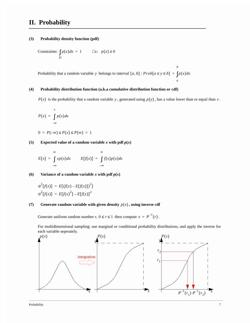
(7) Generate random variable with given density , using inverse cdf

Generate uniform random number r, then compute .

For multidimensional sampling: use marginal or conditional probability distributions, and apply the inverse foreach variable seperately.

p x( ) xd

D

∫ 1= x: p x( ) 0≥∀

y a b,[ ] Prob a y b≤ ≤[ ] p x( ) xd

a

b

∫=

P x( ) y p y( ) x

P x( ) p x( ) xd

∞–

x

∫=

0 P ∞–( ) P x( ) P ∞( )≤≤ 1= =

E x[ ] xp x( ) xd

∞–

∞

∫= E f x( )[ ] f x( )p x( ) xd

∞–

∞

∫=

σ2f x( )[ ] E f x( ) E f x( )[ ]–( )2[ ]=

σ2f x( )[ ] E f x( )2[ ] E f x( )[ ] 2

–=

p x( )

0 r 1≤ ≤ x P1–

r( )=

p x( ) P x( ) P x( )1 1

x xx

r1

r2

P1–

r1( ) P1–

r2( )

integration

Probability 8

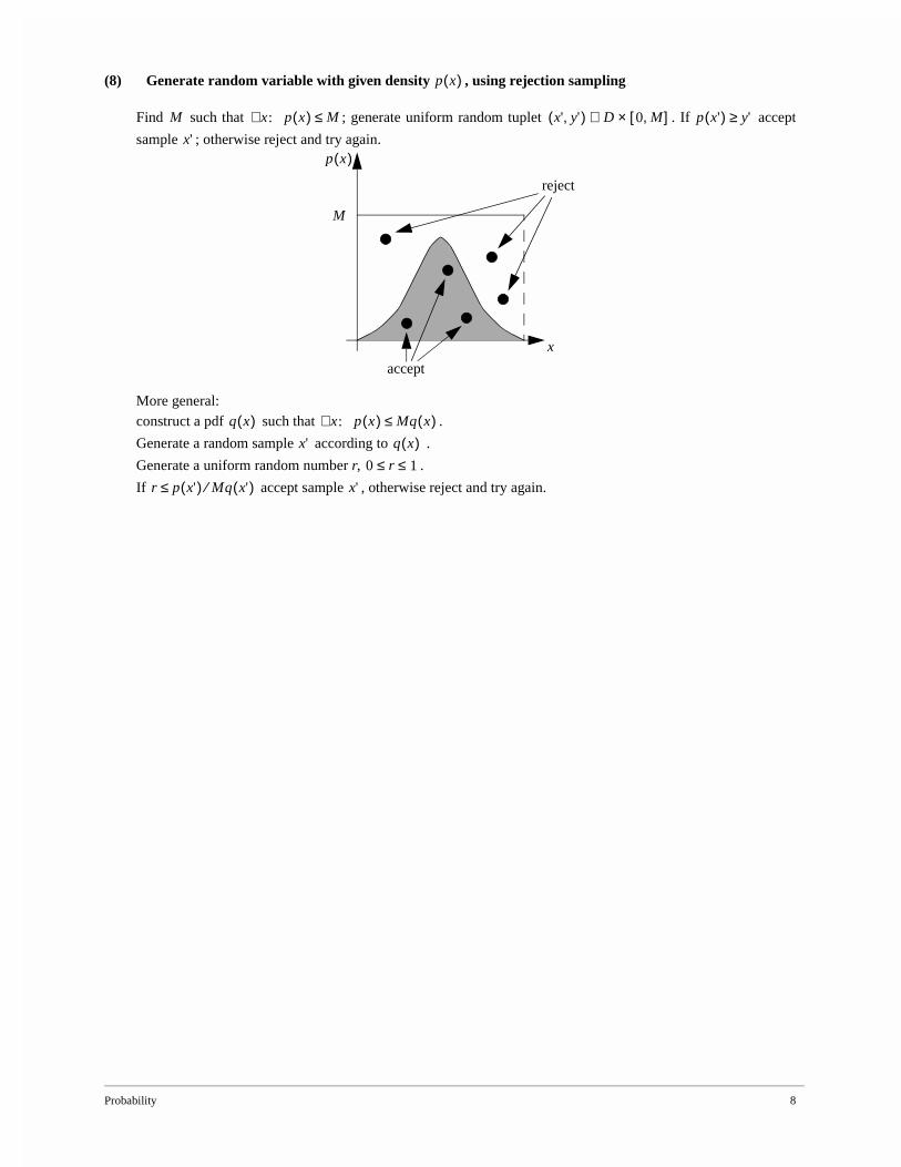
(8) Generate random variable with given density , using rejection sampling

Find such that ; generate uniform random tuplet . If accept

sample ; otherwise reject and try again.

More general:construct a pdf such that .

Generate a random sample according to .

Generate a uniform random number r, .

If accept sample , otherwise reject and try again.

p x( )

M x: p x( ) M≤∀ x' y',( ) D 0 M,[ ]×∈ p x'( ) y'≥x'

p x( )

x

M

accept

reject

q x( ) x: p x( ) Mq x( )≤∀x' q x( )

0 r 1≤ ≤r p x'( ) Mq x'( )⁄≤ x'

Geometry 9

III. Geometry

Notations:

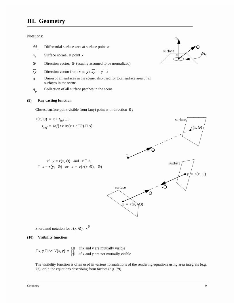
(9) Ray casting function

Closest surface point visible from (any) point in direction :

Shorthand notation for :

(10) Visibility function

The visibility function is often used in various formulations of the rendering equations using area integrals (e.g.73), or in the equations describing form factors (e.g. 79).

Differential surface area at surface point

Surface normal at point

Direction vector: (usually assumed to be normalized)

Direction vector from to :

Union of all surfaces in the scene, also used for total surface area of all surfaces in the scene.

Collection of all surface patches in the scene

x

Θ

nx

dAxsurface

dAx x

nx x

Θ Θ

xy x y xy y x–=

A

Ap

x Θ

xΘ

surface

r x Θ,( )

r x Θ,( ) x tinf Θ⋅+=

tinf inf t 0: x t Θ⋅+( ) A∈> =

Θ

surface

surface -Θ

y r x Θ,( )=

x r y Θ–,( )=

if y r x Θ,( )= and x A∈ x r y Θ–,( )= or x⇒ r r x Θ,( ) Θ–,( )=

r x Θ,( ) xΘ

x y A∈,∀ : V x y,( )1 if x and y are mutually visible

0 if x and y are not mutually visible

=

Geometry 10

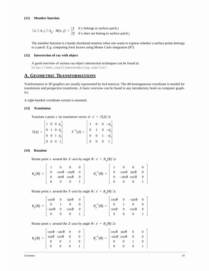
(11) Member function

The member function is a handy shorthand notation when one wants to express whether a surface points belongsto a patch. E.g. computing form factors using Monte Carlo integration (87).

(12) Intersection of ray with object

A good overview of various ray-object intersection techniques can be found at:http://www.realtimerendering.com/int/

A. GEOMETRIC TRANSFORMATIONS

Tranformation in 3D graphics are usually represented by 4x4 matrices. The 4th homogeneous coordinate is needed fortranslations and perspective transforms. A basic overview can be found in any introductory book on computer graph-ics.

A right-handed coordinate system is assumed.

(13) Translation

Translate a point by translation vector :

(14) Rotation

Rotate point around the -axis by angle :

Rotate point around the -axis by angle :

Rotate point around the -axis by angle :

x A j Ap∈,∈∀ : M x j,( )1 if x belongs to surface patch j

0 if x does not belong to surface patch j

=

x d x' T d( ) x⋅=

T d( )

1 0 0 dx

0 1 0 dy

0 0 1 dz

0 0 0 1

= T1–

d( )

1 0 0 d– x

0 1 0 d– y

0 0 1 d– z

0 0 0 1

=

x X θ x' Rx θ( ) x⋅=

Rx θ( )

1 0 0 0

0 θcos θsin– 0

0 θsin θcos 0

0 0 0 1

= Rx1– θ( )

1 0 0 0

0 θcos θsin 0

0 θsin– θcos 0

0 0 0 1

=

x Y θ x' Ry θ( ) x⋅=

Ry θ( )

θcos 0 θsin 0

0 1 0 0

θsin– 0 θcos 0

0 0 0 1

= Ry1– θ( )

θcos 0 θsin– 0

0 1 0 0

θsin 0 θcos 0

0 0 0 1

=

x Z θ x' Rz θ( ) x⋅=

Rz θ( )

θcos θsin– 0 0

θsin θcos 0 0

0 0 1 0

0 0 0 1

= Rz1– θ( )

θcos θsin 0 0

θsin– θcos 0 0

0 0 1 0

0 0 0 1

=

Geometry 11

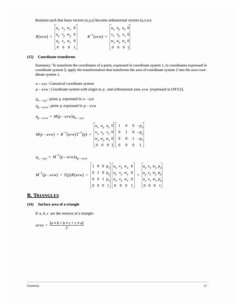
Rotation such that basis vectors (x,y,z) become orthonormal vectors (u,v,w):

(15) Coordinate transforms

Summary: To transform the coordinates of a point, expressed in coordinate system 1, to coordinates expressed incoordinate system 2; apply the transformation that transforms the axes of coordinate system 2 into the axes coor-dinate system 1.

: Canonical coordinate system

: Coordinate system with origin in , and orthonormal axes (expressed in OXYZ).

: point expressed in

: point expressed in

B. TRIANGLES

(16) Surface area of a triangle

If are the vertices of a triangle:

R uvw( )

ux vx wx 0

uy vy wy 0

uz vz wz 0

0 0 0 1

= R1–

uvw( )

ux uy uz 0

vx vy vz 0

wx wy wz 0

0 0 0 1

=

o xyz–

p uvw– p uvw

qo xyz– q o xyz–

qp uvw– q p uvw–

qp uvw– M p uvw–( )qo xyz–=

M p uvw–( ) R1–

uvw( )T1–

p( )

ux uy uz 0

vx vy vz 0

wx wy wz 0

0 0 0 1

1 0 0 p– x

0 1 0 p– y

0 0 1 p– z

0 0 0 1

= =

qo xyz– M1–

p uvw–( )qp uvw–=

M1–

p uvw–( ) T p( )R uvw( )

1 0 0 px

0 1 0 py

0 0 1 pz

0 0 0 1

ux vx wx 0

uy vy wy 0

uz vz wz 0

0 0 0 1

ux vx wx px

uy vy wy py

uz vz wz pz

0 0 0 1

= = =

a b c, ,

areaa b× b c× c a×+ +

2-----------------------------------------------------=

Geometry 12

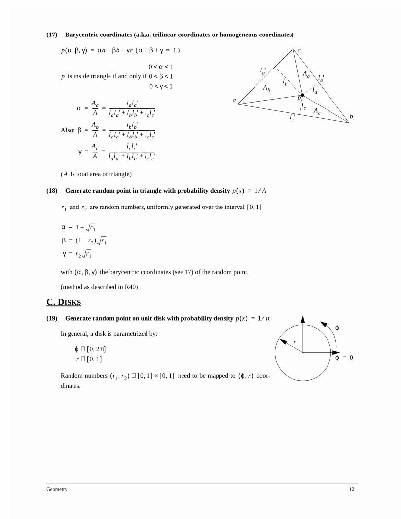
(17) Barycentric coordinates (a.k.a. trilinear coordinates or homogeneous coordinates)

( )

is inside triangle if and only if

Also:

( is total area of triangle)

(18) Generate random point in triangle with probability density

and are random numbers, uniformly generated over the interval

with the barycentric coordinates (see 17) of the random point.

(method as described in R40)

C. DISKS

(19) Generate random point on unit disk with probability density

In general, a disk is parametrized by:

Random numbers need to be mapped to coor-

dinates.

a

c

b

p

Aa

Ab

Ac

la

lb

lc

lb'la'

lc'

p α β γ, ,( ) αa βb γc+ += α β γ+ + 1=

p

0 α 1< <0 β 1< <0 γ 1< <

αAa

A------

lala'

lala' lblb' lclc'+ +------------------------------------------= =

βAb

A------

lblb'

lala' lblb' lclc'+ +------------------------------------------= =

γAc

A------

lclc'

lala' lblb' lclc'+ +------------------------------------------= =

A

p x( ) 1 A⁄=

r1 r2 0 1,[ ]

α 1 r1–=

β 1 r2–( ) r1=

γ r2 r1=

α β γ, ,( )

ϕ

ϕ 0=

r

p x( ) 1 π⁄=

ϕ 0 2π,[ ]∈r 0 1,[ ]∈

r1 r2,( ) 0 1,[ ] 0 1,[ ]×∈ ϕ r,( )

Geometry 13

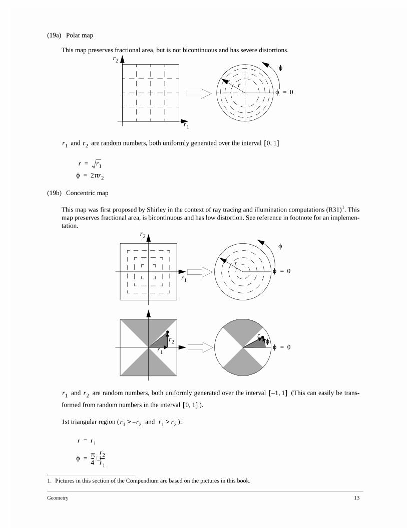
(19a) Polar map

This map preserves fractional area, but is not bicontinuous and has severe distortions.

and are random numbers, both uniformly generated over the interval

(19b) Concentric map

This map was first proposed by Shirley in the context of ray tracing and illumination computations (R31)1. Thismap preserves fractional area, is bicontinuous and has low distortion. See reference in footnote for an implemen-tation.

and are random numbers, both uniformly generated over the interval (This can easily be trans-

formed from random numbers in the interval ).

1st triangular region ( ):

1. Pictures in this section of the Compendium are based on the pictures in this book.

r1

r2

ϕ 0=

ϕ

r

r1 r2 0 1,[ ]

r r1=

ϕ 2πr2=

r1

r2r

ϕ

r1

r2

ϕ 0=

ϕ

r

ϕ 0=

r1 r2 1– 1,[ ]

0 1,[ ]

r1 r– 2> and r1 r2>

r r1=

ϕ π4---

r2

r1----⋅=

Geometry 14

2nd triangular region ( ):

3rd triangular region ( ):

4th triangular region ( ):

r1 r2< and r1 r2–>

r r2=

ϕ π4--- 2

r1

r2----–

⋅=

r1 r– 2< and r1 r2<

r r– 1=

ϕ π4--- 4

r2

r1----+

⋅=

r1 r2> and r1 r2–<

r r– 2=

ϕ π4--- 6

r1

r2----–

⋅=

Hemispherical Geometry 15

IV. Hemispherical Geometry

A. GENERAL

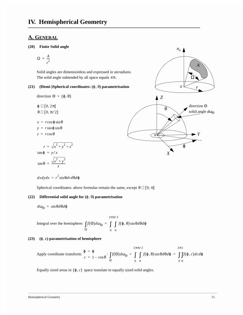
(20) Finite Solid angle

Solid angles are dimensionless and expressed in steradians.The solid angle subtended by all space equals .

(21) (Hemi-)Spherical coordinates: (ϕ, θ) parametrisation

direction

Spherical coordinates: above formulas remain the same, except

(22) Differential solid angle for (ϕ, θ) parametrisation

Integral over the hemisphere:

(23) (ϕ, c) parametrisation of hemisphere

Apply coordinate transform: :

Equally sized areas in space translate to equally sized solid angles.

x

nx

r

A

Ω

Ω A

r2

----=

4π

x

solid angle dωΘ

direction Θ

ϕ

θ

Z

X

Y

Θ ϕ θ,( )=

ϕ 0 2π,[ ]∈θ 0 π 2⁄,[ ]∈

x r ϕ θsincos=

y r ϕ θsinsin=

z r θcos=

r x2

y2

z2

+ +=

ϕtan y x⁄=

θtanx

2y

2+

z---------------------=

dxdydz r2 θdrdθdϕsin=

θ 0 π,[ ]∈

dωΘ θdθdϕsin=

f Θ( )dωΘΩ∫ f ϕ θ,( ) θdθdϕsin

0

π 2⁄

∫0

2π

∫=

ϕ ϕ=

c 1 θcos–=f Θ( )dωΘ

Ω∫ f ϕ θ,( ) θdθdϕsin

0

π 2⁄

∫0

2π

∫ f ϕ c,( )dcdϕ

0

1

∫0

2π

∫= =

ϕ c,( )

Hemispherical Geometry 16

(24) (ξ1, ξ2) parametrisation of hemisphere

Apply coordinate transform: :

Equally sized areas in space translate to equally sized, cosine-weighted solid angles.

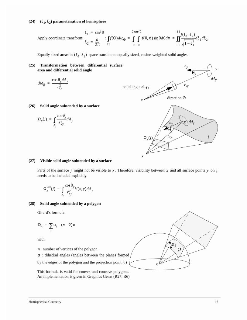
(25) Transformation between differential surfacearea and differential solid angle

(26) Solid angle subtended by a surface

(27) Visible solid angle subtended by a surface

Parts of the surface might not be visible to . Therefore, visibility between and all surface points on needs to be included explicitly.

(28) Solid angle subtended by a polygon

Girard’s formula:

with:

: number of vertices of the polygon

: dihedral angles (angles between the planes formed

by the edges of the polygon and the projection point )

This formula is valid for convex and concave polygons.An implementation is given in Graphics Gems (R27, R6).

ξ1 θsin2=

ξ2ϕ

2π------=

f Θ( )dωΘΩ∫ f θ ϕ,( ) θdθdϕsin

0

π 2⁄

∫0

2π

∫f ξ1 ξ2,( )

1 ξ12

–---------------------dξ1dξ2

0

1

∫0

1

∫= =

ξ1 ξ2,( )

x

yny

θy

rxy

direction Θ

solid angle dωΘ

dAydωΘ

θydAycos

rxy2

------------------------=

x

yny

θy

rxy

dAy

Ωx j( ) j

Ωx j( )θycos

rxy2

--------------dAy

Aj

∫=

j x x y j

Ωxvis

j( )θycos

rxy2

--------------V x y,( )dAy

Aj

∫=

αiΩ

x

Ωx α i

i

∑ n 2–( )π–=

n

α i

x

Hemispherical Geometry 17

(29) Tangent-sphere function

In the context of global illumination, one is often interested in the cosine of the angle between a direction on

the hemisphere and the normal vector at a surface point , but only if the direction is located at the same side

of the surface of . If is ‘below’ the surface, the value is . Some authors (R34) introduce the ‘tangent-

sphere’ function for this purpose:

In this document, the notation is often used.

(30) Useful integrals (cosine lobes) over the hemisphere (see also 33, 34, 35 and 36)

Integrals of cosine lobes are useful because many BRDF models (e.g. Lafortune model, see 70) make use ofthese lobes, although usually not centered around the normal.

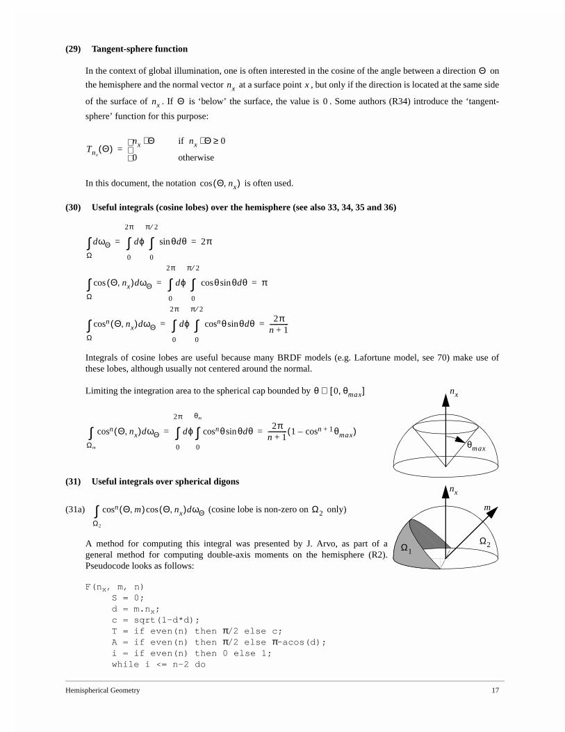
Limiting the integration area to the spherical cap bounded by

(31) Useful integrals over spherical digons

(31a) (cosine lobe is non-zero on only)

A method for computing this integral was presented by J. Arvo, as part of ageneral method for computing double-axis moments on the hemisphere (R2).Pseudocode looks as follows:

F(nx, m, n)S = 0;d = m.nx;c = sqrt(1-d*d);T = if even(n) then π/2 else c;A = if even(n) then π/2 else π-acos(d);i = if even(n) then 0 else 1;while i <= n-2 do

Θnx x

nx Θ 0

TnxΘ( )

nx Θ⋅

0

=if nx Θ⋅ 0≥

otherwise

Θ nx,( )cos

dωΘΩ∫ dϕ θdθsin

0

π 2⁄

∫0

2π

∫ 2π= =

Θ nx,( )dcos ωΘΩ∫ dϕ θ θdθsincos

0

π 2⁄

∫0

2π

∫ π= =

Θ nx,( )cosn dωΘΩ∫ dϕ θcosn θdθsin

0

π 2⁄

∫0

2π

∫ 2πn 1+------------= =

θmax

nxθ 0 θmax,[ ]∈

Θ nx,( )cosn dωΘΩm

∫ dϕ θcosn θdθsin

0

θm

∫0

2π

∫ 2πn 1+------------ 1 θmaxcosn 1+–( )= =

nx

Ω2

m

Ω1

Θ m,( )cosn Θ nx,( )dcos ωΘΩ2

∫ Ω2

Hemispherical Geometry 18

S = S+T;T = T*c*c*(i+1)/(i+2);i = i+2;endwhile

return 2*(T + d*A + d*d*S)/(n+2)end

(31b) (cosine lobe is non-zero on only)

An expression can be derived from the same paper (although this form is not explicitly mentioned):

where:

(32) Dirac-impulse on hemisphere (see also 1)

such that:

B. GENERATING POINTS AND DIRECTIONS ON THE (HEMI)SPHERE

Generating random directions over the hemisphere is a fundamental operations in most Monte Carlo-based renderingalgorithms. The rendering equation (see section IX) is usually expressed as an integral over the hemisphere, so sam-pling the hemispherical domain requires generating directions over the hemisphere.

and are random numbers, uniformly generated over the interval . Some of the formulas can be simplified

by substituting a uniform random variable with or vice versa. Since both have the distribution, the resultingdistribution of directions is not affected.

Θ m,( )cosn dωΘΩ2

∫ Ω2

n even: Θ m,( )cosn dωΘΩ2

∫2 π θm–( ) θm θmsinn 1– Fn 1– θmsinn 3– Fn 3– … θmsin F1+ + +[ ]cos+

n 1+------------------------------------------------------------------------------------------------------------------------------------------------------------------------------=

n odd: Θ m,( )cosn dωΘΩ2

∫π θm θmsinn 1– Fn 1– θmsinn 3– Fn 3– … F0+ + +[ ]cos+

n 1+------------------------------------------------------------------------------------------------------------------------------------------=

θm m nx⋅( )acos=

Fnn 1–

n------------F

n 2–= F0 π= F1 2=

δ Θ1 Θ–( ) δ θ1cos θcos–( )δ ϕ1 ϕ–( )=

Θ1 θ1 ϕ1,( )=

Θ θ ϕ,( )=

δ Θ1 Θ–( )f Θ( )dωΘΩ∫ dϕδ ϕ1 ϕ–( ) d θcos( )δ θ1cos θcos–( )f ϕ θ,( )

0

π 2⁄

∫0

2π

∫=

dϕδ ϕ1 ϕ–( )f ϕ θ1,( )

0

2π

∫ f ϕ1 θ1,( ) f Θ1( )= = =

r1 r2 0 1,[ ]

r 1 r–

Hemispherical Geometry 19

(33) Generate random point on sphere with density

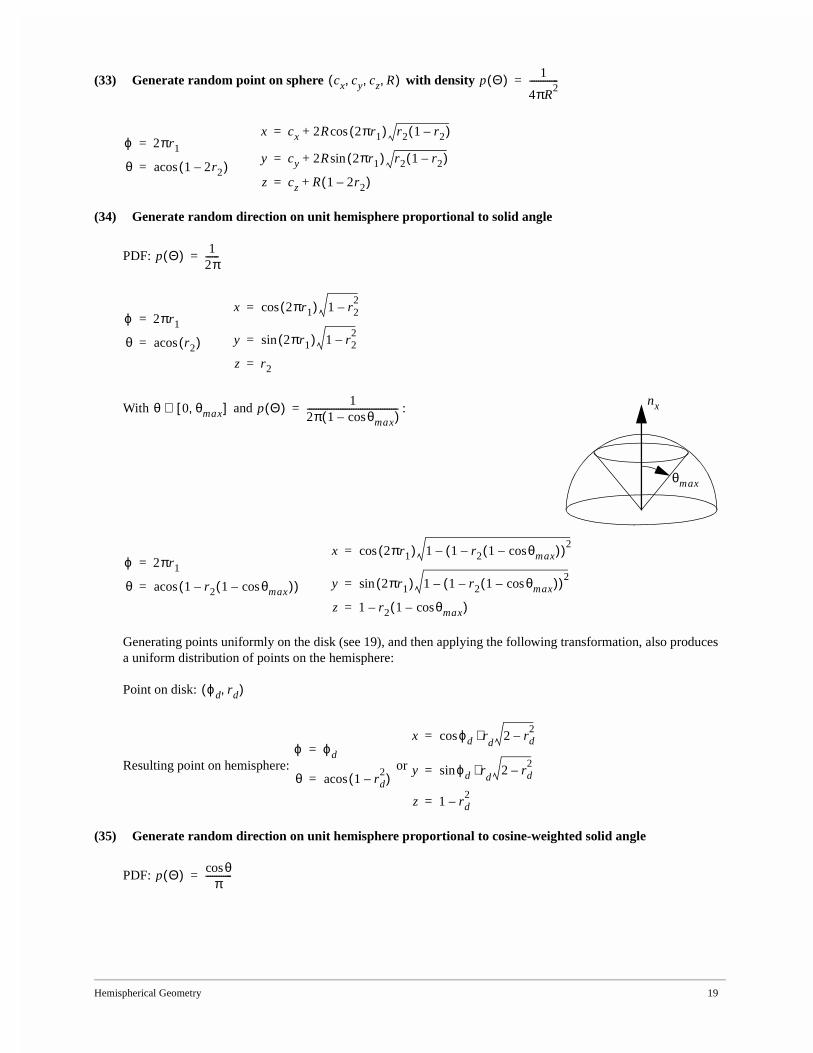
(34) Generate random direction on unit hemisphere proportional to solid angle

PDF:

With and :

Generating points uniformly on the disk (see 19), and then applying the following transformation, also producesa uniform distribution of points on the hemisphere:

Point on disk:

Resulting point on hemisphere: or

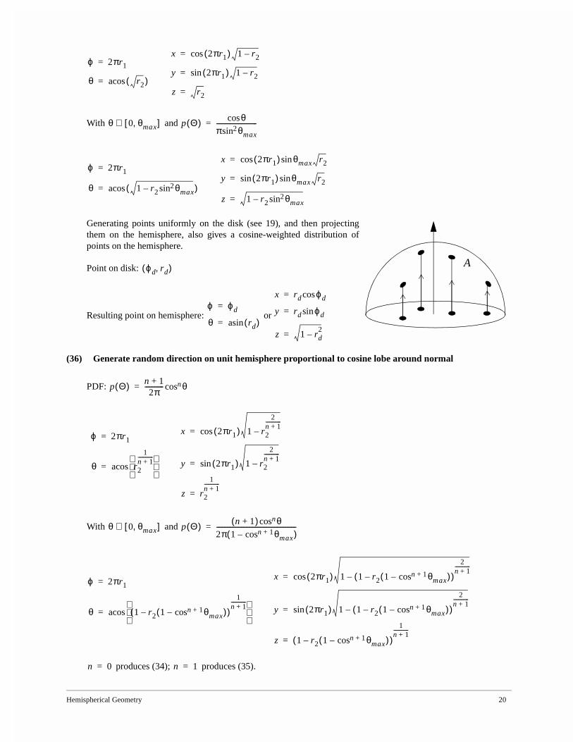
(35) Generate random direction on unit hemisphere proportional to cosine-weighted solid angle

PDF:

cx cy cz R, , ,( ) p Θ( ) 1

4πR2

-------------=

ϕ 2πr1=

θ 1 2r2–( )acos=

x cx 2R 2πr1( ) r2 1 r2–( )cos+=

y cy 2R 2πr1( )sin r2 1 r2–( )+=

z cz R 1 2r2–( )+=

p Θ( ) 12π------=

ϕ 2πr1=

θ r2( )acos=

x 2πr1( ) 1 r22

–cos=

y 2πr1( )sin 1 r22

–=

z r2=

θmax

nxθ 0 θmax,[ ]∈ p Θ( ) 12π 1 θmaxcos–( )-----------------------------------------=

ϕ 2πr1=

θ 1 r– 2 1 θmaxcos–( )( )acos=

x 2πr1( ) 1 1 r– 2 1 θmaxcos–( )( )2–cos=

y 2πr1( )sin 1 1 r– 2 1 θmaxcos–( )( )2–=

z 1 r– 2 1 θmaxcos–( )=

ϕd rd,( )

ϕ ϕ d=

θ 1 rd2

–( )acos=

x ϕdcos r⋅d

2 rd2

–=

y ϕdsin r⋅d

2 rd2

–=

z 1 rd2

–=

p Θ( ) θcosπ

------------=

Hemispherical Geometry 20

With and

Generating points uniformly on the disk (see 19), and then projectingthem on the hemisphere, also gives a cosine-weighted distribution ofpoints on the hemisphere.

Point on disk:

Resulting point on hemisphere: or

(36) Generate random direction on unit hemisphere proportional to cosine lobe around normal

PDF:

With and

produces (34); produces (35).

ϕ 2πr1=

θ r2( )acos=

x 2πr1( ) 1 r2–cos=

y 2πr1( )sin 1 r2–=

z r2=

θ 0 θmax,[ ]∈ p Θ( ) θcos

π θmaxsin2--------------------------=

ϕ 2πr1=

θ 1 r– 2 θmaxsin2( )acos=

x 2πr1( ) θmaxsin r2cos=

y 2πr1( )sin θmaxsin r2=

z 1 r– 2 θmaxsin2=

Aϕd rd,( )

ϕ ϕ d=

θ rd( )asin=

x rd ϕdcos=

y rd ϕdsin=

z 1 rd2

–=

p Θ( ) n 1+2π

------------ θcosn=

ϕ 2πr1=

θ r2

1n 1+------------

acos=

x 2πr1( ) 1 r2

2n 1+------------

–cos=

y 2πr1( )sin 1 r2

2n 1+------------

–=

z r2

1n 1+------------

=

θ 0 θmax,[ ]∈ p Θ( ) n 1+( ) θcosn

2π 1 θmaxcosn 1+–( )---------------------------------------------------=

ϕ 2πr1=

θ 1 r– 2 1 θmaxcosn 1+–( )( )

1n 1+------------

acos=

x 2πr1( ) 1 1 r– 2 1 θmaxcosn 1+–( )( )

2n 1+------------

–cos=

y 2πr1( )sin 1 1 r– 2 1 θmaxcosn 1+–( )( )

2n 1+------------

–=

z 1 r– 2 1 θmaxcosn 1+–( )( )

1n 1+------------

=

n 0= n 1=

Hemispherical Geometry 21

(37) Generate uniform random direction on a spherical triangle

See the paper published by J. Arvo in SIGGRAPH 95 for a complete formula and algorithm (R1).

(38) Generate random direction on spherical digon; density proportional to cosnα; α angle from off-normalaxis

1. Generate direction on unit hemisphere proportional to using (36).2. Transform direction by transforming normal to off-normal axis.3. If transformed direction has angle greater then π/2 with normal, reject direction and try again.

4. Compute correct pdf-value by normalizing using (31b).

θcosn

αcosn

Monte Carlo Integration, 22

V. Monte Carlo Integration1,2

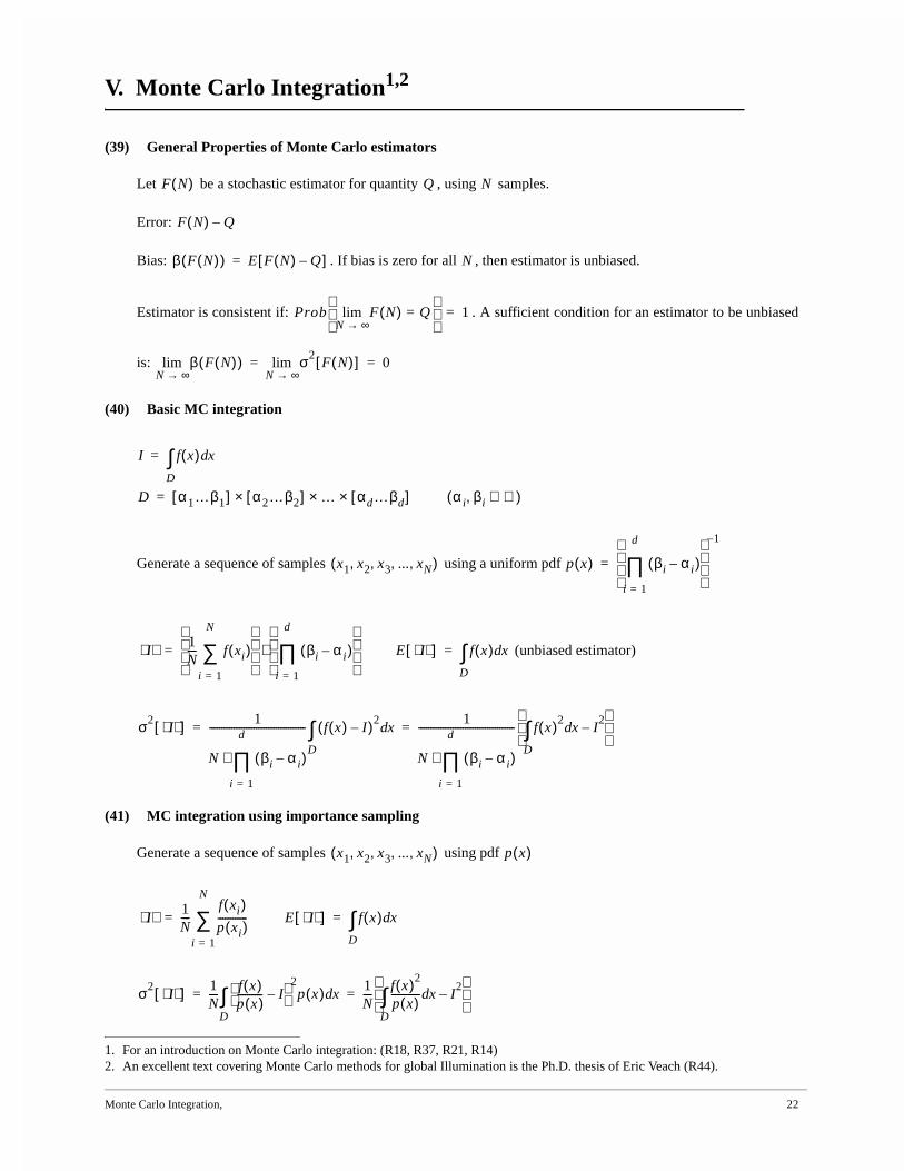
(39) General Properties of Monte Carlo estimators

Let be a stochastic estimator for quantity , using samples.

Error:

Bias: . If bias is zero for all , then estimator is unbiased.

Estimator is consistent if: . A sufficient condition for an estimator to be unbiased

is:

(40) Basic MC integration

Generate a sequence of samples using a uniform pdf

(unbiased estimator)

(41) MC integration using importance sampling

Generate a sequence of samples using pdf

1. For an introduction on Monte Carlo integration: (R18, R37, R21, R14)2. An excellent text covering Monte Carlo methods for global Illumination is the Ph.D. thesis of Eric Veach (R44).

F N( ) Q N

F N( ) Q–

β F N( )( ) E F N( ) Q–[ ]= N

Prob F N( )N ∞→lim Q=

1=

β F N( )( )N ∞→lim σ2

F N( )[ ]N ∞→lim 0= =

I f x( ) xd

D

∫=

D α1…β1[ ] α 2…β2[ ] …× αd…βd[ ]××= α i βi, ℜ∈( )

x1 x2 x3 ... xN, , , ,( ) p x( ) βi α i–( )

i 1=

d

∏ 1–

=

I⟨ ⟩ 1N---- f xi( )

i 1=

N

∑

βi α i–( )

i 1=

d

∏

⋅= E I⟨ ⟩[ ] f x( ) xd

D

∫=

σ2I⟨ ⟩[ ] 1

N βi α i–( )

i 1=

d

∏⋅

--------------------------------------- f x( ) I–( )2xd

D

∫ 1

N βi α i–( )

i 1=

d

∏⋅

--------------------------------------- f x( )2xd

D

∫ I2

–

= =

x1 x2 x3 ... xN, , , ,( ) p x( )

I⟨ ⟩ 1N----

f xi( )p xi( )------------

i 1=

N

∑= E I⟨ ⟩[ ] f x( ) xd

D

∫=

σ2I⟨ ⟩[ ] 1

N---- f x( )

p x( )---------- I–

2p x( ) xd

D

∫ 1N---- f x( )2

p x( )------------ xd

D

∫ I2

–

= =

Monte Carlo Integration, 23

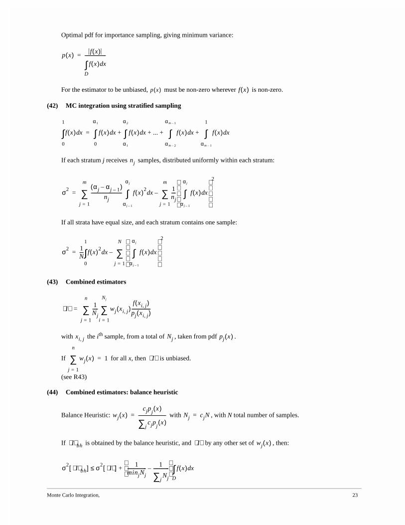
Optimal pdf for importance sampling, giving minimum variance:

For the estimator to be unbiased, must be non-zero wherever is non-zero.

(42) MC integration using stratified sampling

If each stratum j receives samples, distributed uniformly within each stratum:

If all strata have equal size, and each stratum contains one sample:

(43) Combined estimators

with the ith sample, from a total of , taken from pdf .

If for all x, then is unbiased.

(see R43)

(44) Combined estimators: balance heuristic

Balance Heuristic: with , with N total number of samples.

If is obtained by the balance heuristic, and by any other set of , then:

p x( ) f x( )

f x( ) xd

D

∫-------------------=

p x( ) f x( )

f x( ) xd

0

1

∫ f x( ) xd

0

α1

∫ f x( ) xd

α1

α2

∫ ... f x( ) xd

αm 2–

αm 1–

∫ f x( ) xd

αm 1–

1

∫+ + + +=

nj

σ2 α j α j 1––( )nj

---------------------------- f x( )2xd

α j 1–

α j

∫j 1=

m

∑ 1nj---- f x( ) xd

α j 1–

α j

∫ 2

j 1=

m

∑–=

σ2 1N---- f x( )2

xd

0

1

∫ f x( ) xd

α j 1–

α j

∫ 2

j 1=

N

∑–=

I⟨ ⟩ 1Nj----- wj xi j,( )

f xi j,( )pj xi j,( )-----------------

i 1=

Nj

∑j 1=

n

∑=

xi j, Nj pj x( )

wj x( )

j 1=

n

∑ 1= I⟨ ⟩

wj x( )cjpj

x( )

cjpjx( )

j∑-------------------------= Nj cjN=

I⟨ ⟩ bh I⟨ ⟩ wj x( )

σ2I⟨ ⟩ bh[ ] σ 2

I⟨ ⟩[ ] 1minjNj----------------- 1

Njj∑--------------–

f x( ) xd

D

∫+≤

Monte Carlo Integration, 24

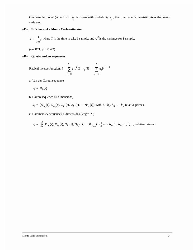
One sample model ( ): if is cosen with probability , then the balance heuristic gives the lowest

variance.

(45) Efficiency of a Monte Carlo estimator

where T is the time to take 1 sample, and is the variance for 1 sample.

(see R21, pp. 91-92)

(46) Quasi-random sequences

Radical inverse function:

a. Van der Corput sequence

b. Halton sequence ( dimensions)

with relative primes.

c. Hammersley sequence ( dimensions, length )

with relative primes.

N 1= pj cj

ε 1

Tσ2---------= σ2

i ajbj

j 0=

∞

∑= Φb i( )⇒ ajbj– 1–

j 0=

∞

∑=

xi Φb i( )=

s

xi Φb1i( ) Φb2

i( ) Φb3i( ) Φb4

i( ) … Φ, bsi( ),,,,( )= b1 b2 b3 … bs, , , ,

s N

xiiN---- Φb1

, i( ) Φb2i( ) Φb3

i( ) Φb4i( ) … Φ, bs 1–

i( ),,,, = b1 b2 b3 … bs 1–, , , ,

Radiometry & Photometry 25

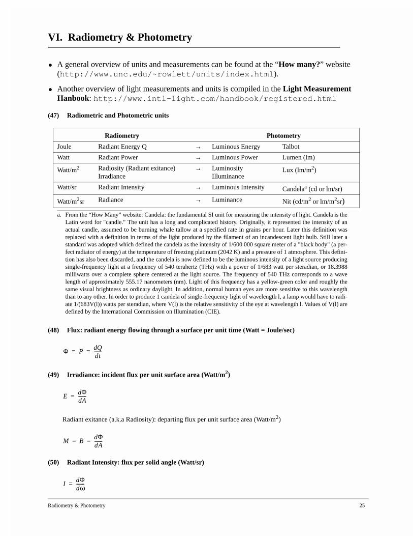
VI. Radiometry & Photometry

• A general overview of units and measurements can be found at the “How many?” website (http://www.unc.edu/~rowlett/units/index.html).

• Another overview of light measurements and units is compiled in the Light Measurement Hanbook: http://www.intl-light.com/handbook/registered.html

(47) Radiometric and Photometric units

(48) Flux: radiant energy flowing through a surface per unit time (Watt = Joule/sec)

(49) Irradiance: incident flux per unit surface area (Watt/m2)

Radiant exitance (a.k.a Radiosity): departing flux per unit surface area (Watt/m2)

(50) Radiant Intensity: flux per solid angle (Watt/sr)

Radiometry Photometry

Joule Radiant Energy Q → Luminous Energy Talbot

Watt Radiant Power → Luminous Power Lumen (lm)

Watt/m2 Radiosity (Radiant exitance)Irradiance

→ LuminosityIlluminance

Lux (lm/m2)

Watt/sr Radiant Intensity → Luminous Intensity Candelaa (cd or lm/sr)

a. From the “How Many” website: Candela: the fundamental SI unit for measuring the intensity of light. Candela is theLatin word for "candle." The unit has a long and complicated history. Originally, it represented the intensity of anactual candle, assumed to be burning whale tallow at a specified rate in grains per hour. Later this definition wasreplaced with a definition in terms of the light produced by the filament of an incandescent light bulb. Still later astandard was adopted which defined the candela as the intensity of 1/600 000 square meter of a "black body" (a per-fect radiator of energy) at the temperature of freezing platinum (2042 K) and a pressure of 1 atmosphere. This defini-tion has also been discarded, and the candela is now defined to be the luminous intensity of a light source producingsingle-frequency light at a frequency of 540 terahertz (THz) with a power of 1/683 watt per steradian, or 18.3988milliwatts over a complete sphere centered at the light source. The frequency of 540 THz corresponds to a wavelength of approximately 555.17 nanometers (nm). Light of this frequency has a yellow-green color and roughly thesame visual brightness as ordinary daylight. In addition, normal human eyes are more sensitive to this wavelengththan to any other. In order to produce 1 candela of single-frequency light of wavelength l, a lamp would have to radi-ate 1/(683V(l)) watts per steradian, where V(l) is the relative sensitivity of the eye at wavelength l. Values of V(l) aredefined by the International Commission on Illumination (CIE).

Watt/m2sr Radiance → Luminance Nit (cd/m2 or lm/m2sr)

Φ PQd

dt-------= =

EΦd

dA-------=

M BΦd

dA-------= =

IΦd

dω-------=

Radiometry & Photometry 26

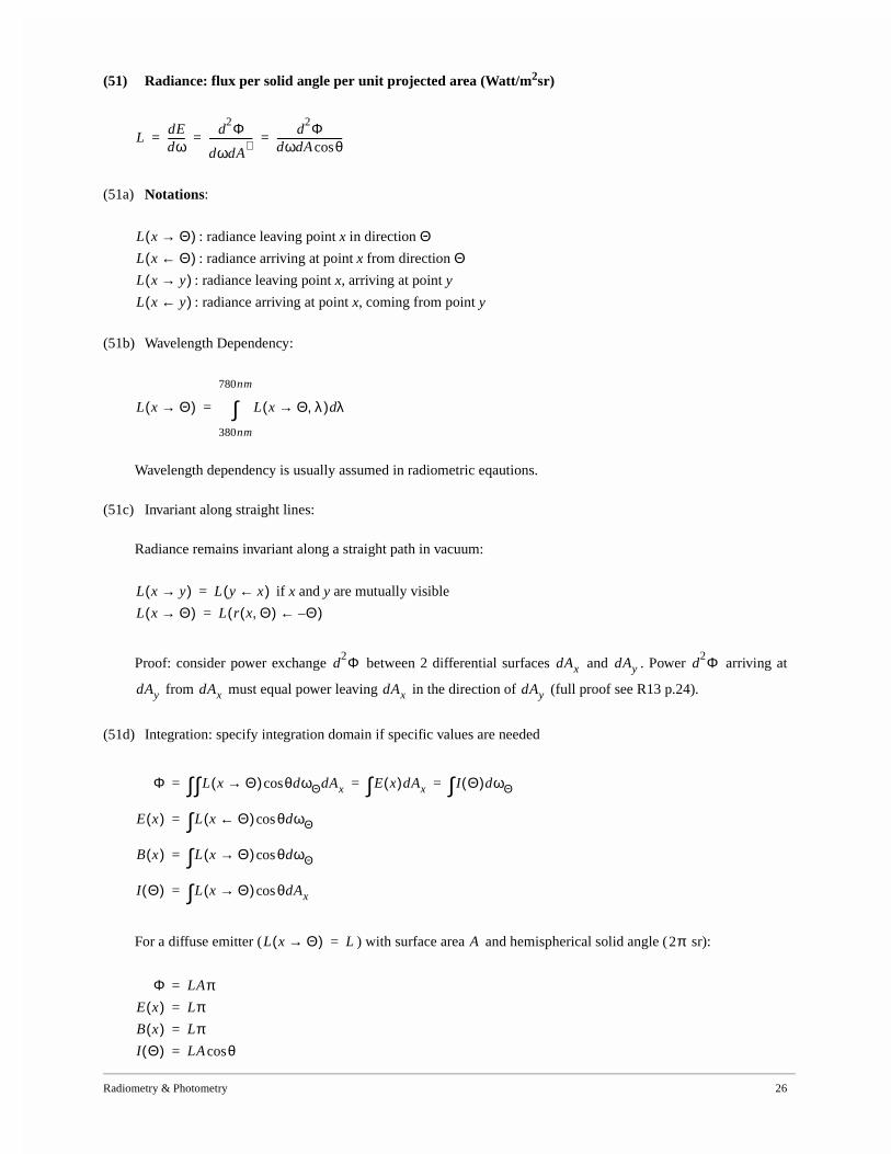
(51) Radiance: flux per solid angle per unit projected area (Watt/m2sr)

(51a) Notations:

: radiance leaving point x in direction Θ: radiance arriving at point x from direction Θ

: radiance leaving point x, arriving at point y

: radiance arriving at point x, coming from point y

(51b) Wavelength Dependency:

Wavelength dependency is usually assumed in radiometric eqautions.

(51c) Invariant along straight lines:

Radiance remains invariant along a straight path in vacuum:

if x and y are mutually visible

Proof: consider power exchange between 2 differential surfaces and . Power arriving at

from must equal power leaving in the direction of (full proof see R13 p.24).

(51d) Integration: specify integration domain if specific values are needed

For a diffuse emitter ( ) with surface area and hemispherical solid angle ( sr):

LdEdω-------

d2Φ

dωdA⊥------------------

d2Φ

dωdA θcos---------------------------= = =

L x Θ→( )L x Θ←( )L x y→( )L x y←( )

L x Θ→( ) L x Θ λ,→( ) λd

380nm

780nm

∫=

L x y→( ) L y x←( )=

L x Θ→( ) L r x Θ,( ) Θ–←( )=

d2Φ dAx dAy d

2Φ

dAy dAx dAx dAy

Φ L x Θ→( ) θdωΘdAxcos∫∫ E x( )dAx∫ I Θ( )dωΘ∫= = =

E x( ) L x Θ←( ) θdωΘcos∫=

B x( ) L x Θ→( ) θdωΘcos∫=

I Θ( ) L x Θ→( ) θdAxcos∫=

L x Θ→( ) L= A 2π

Φ LAπ=

E x( ) Lπ=

B x( ) Lπ=

I Θ( ) LA θcos=

Radiometry & Photometry 27

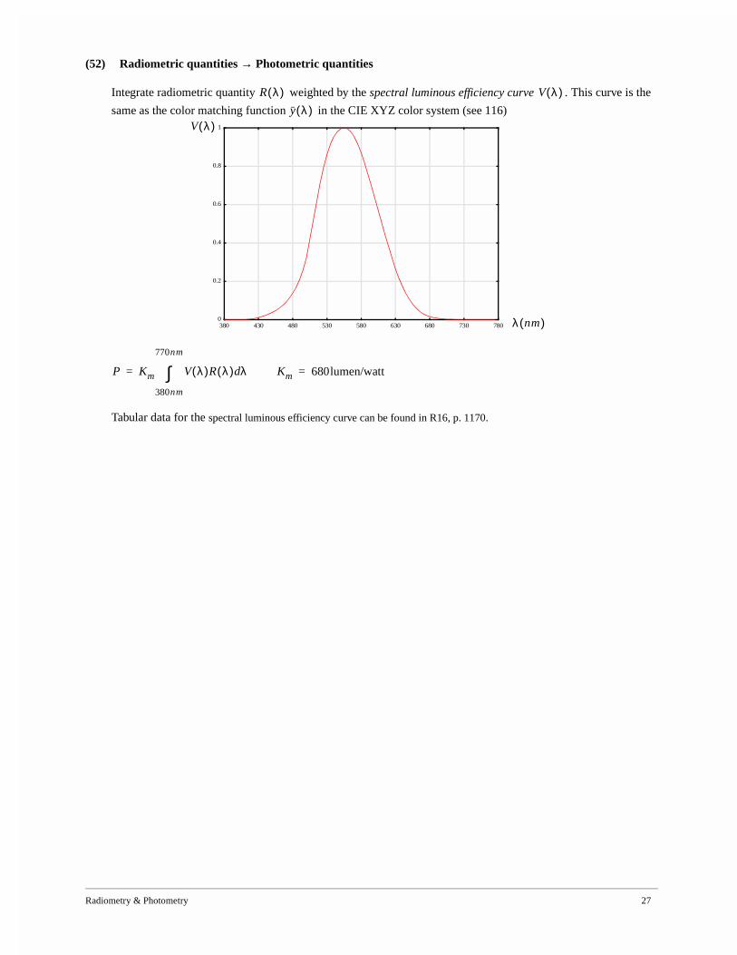
(52) Radiometric quantities → Photometric quantities

Integrate radiometric quantity weighted by the spectral luminous efficiency curve . This curve is the

same as the color matching function in the CIE XYZ color system (see 116)

Tabular data for the spectral luminous efficiency curve can be found in R16, p. 1170.

R λ( ) V λ( )y λ( )

V λ( )

λ nm( )0

0.2

0.4

0.6

0.8

1

380 430 480 530 580 630 680 730 780

P Km V λ( )R λ( ) λd

380nm

770nm

∫= Km 680lumen/watt=

Optics 28

VII. Optics

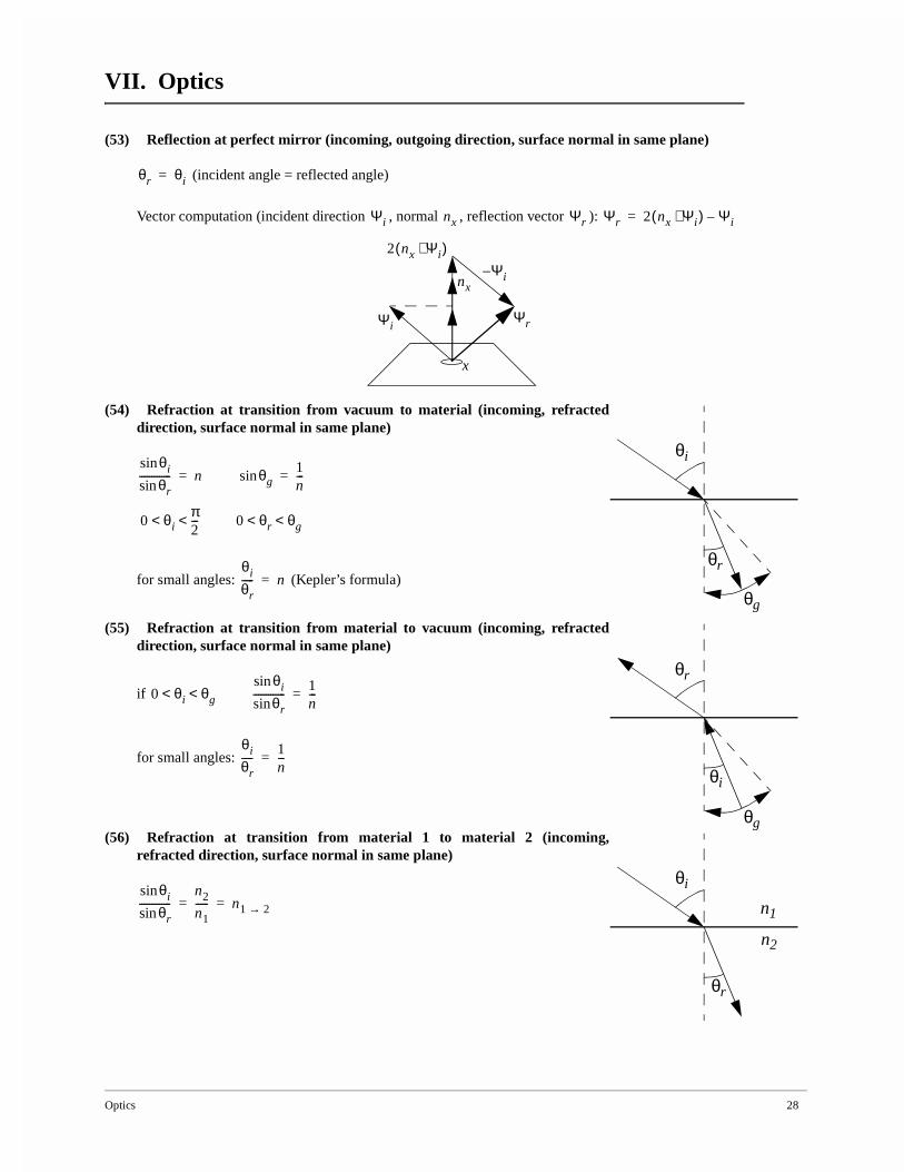
(53) Reflection at perfect mirror (incoming, outgoing direction, surface normal in same plane)

(incident angle = reflected angle)

Vector computation (incident direction , normal , reflection vector ):

(54) Refraction at transition from vacuum to material (incoming, refracteddirection, surface normal in same plane)

for small angles: (Kepler’s formula)

(55) Refraction at transition from material to vacuum (incoming, refracteddirection, surface normal in same plane)

if

for small angles:

(56) Refraction at transition from material 1 to material 2 (incoming,refracted direction, surface normal in same plane)

θr θi=

Ψi nx Ψr Ψr 2 nx Ψi⋅( ) Ψi–=

nx

x

ΨiΨr

2 nx Ψi⋅( )Ψi–

θg

θr

θiθisin

θrsin------------- n= θgsin

1n---=

0 θiπ2---< < 0 θr θg< <

θi

θr----- n=

θg

θr

θi

0 θi θg< <θisin

θrsin------------- 1

n---=

θi

θr-----

1n---=

θr

θi

n1

n2

θisin

θrsin-------------

n2

n1----- n1 2→= =

Optics 29

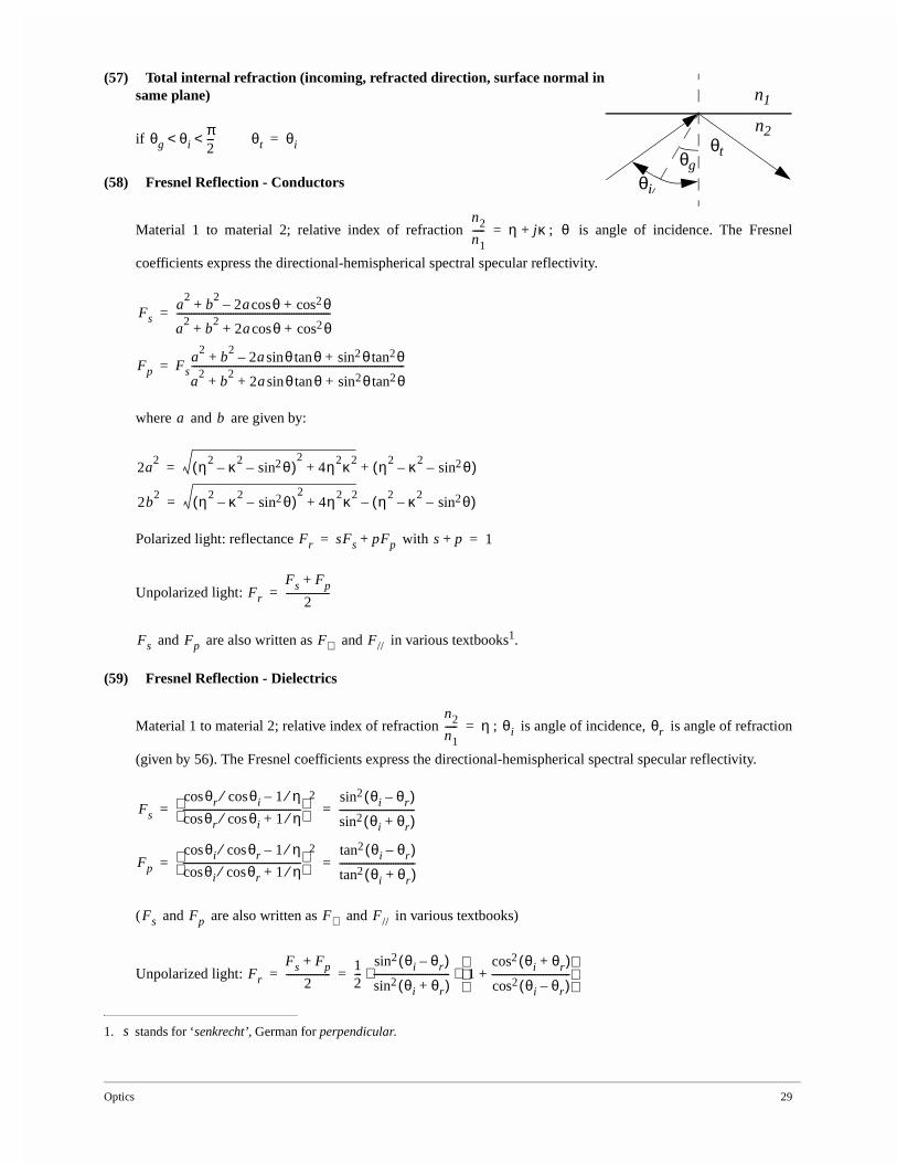
(57) Total internal refraction (incoming, refracted direction, surface normal insame plane)

if

(58) Fresnel Reflection - Conductors

Material 1 to material 2; relative index of refraction ; is angle of incidence. The Fresnel

coefficients express the directional-hemispherical spectral specular reflectivity.

where and are given by:

Polarized light: reflectance with

Unpolarized light:

and are also written as and in various textbooks1.

(59) Fresnel Reflection - Dielectrics

Material 1 to material 2; relative index of refraction ; is angle of incidence, is angle of refraction

(given by 56). The Fresnel coefficients express the directional-hemispherical spectral specular reflectivity.

( and are also written as and in various textbooks)

Unpolarized light:

1. stands for ‘senkrecht’, German for perpendicular.

θt

θi

n1

n2

θg

θg θiπ2---< < θt θi=

n2

n1----- η jκ+= θ

Fsa

2b

22a θcos θcos2+–+

a2

b2

2a θcos θcos2+ + +---------------------------------------------------------------=

Fp Fsa

2b

22a θsin θtan θ θtan2sin2+–+

a2

b2

2a θsin θtan θ θtan2sin2+ + +---------------------------------------------------------------------------------------=

a b

2a2 η2 κ2

– θsin2–( )2

4η2κ2+ η2 κ2

– θsin2–( )+=

2b2 η2 κ2

– θsin2–( )2

4η2κ2+ η2 κ2

– θsin2–( )–=

Fr sFs pFp+= s p+ 1=

Fr

Fs Fp+

2------------------=

Fs Fp F⊥ F//

s

n2

n1----- η= θi θr

Fs

θrcos θicos⁄ 1 η⁄–

θrcos θicos⁄ 1 η⁄+------------------------------------------------

2 θi θr–( )sin2

θi θr+( )sin2-------------------------------= =

Fp

θicos θrcos⁄ 1 η⁄–

θicos θrcos⁄ 1 η⁄+------------------------------------------------

2 θi θr–( )tan2

θi θr+( )tan2-------------------------------= =

Fs Fp F⊥ F//

Fr

Fs Fp+

2------------------

12---

θi θr–( )sin2

θi θr+( )sin2------------------------------- 1

θi θr+( )cos2

θi θr–( )cos2--------------------------------+

⋅ ⋅= =

Optics 30

If , and thus : (also sometimes written as )

(60) Index of Refraction Data Values

A website listing all sort of possible data is at http://www.luxpop.com/

θi 0= θr 0= Fr Fs Fpη 1–η 1+-------------

2= = = F0

Bidirectional Reflectance Distribution Functions (BRDFs) 31

VIII. Bidirectional Reflectance Distribution Functions (BRDFs)

A. GENERAL PROPERTIES

(61) BRDF:

BRDF is dimensionless but is expressed as 1/sr

BTDF = Bidirectional Transmittance Function: similar as BRDF but defined for transmittanceBSDF = combination of 2 BRDFs and 2 BTDFs (one pair for each side of the surface)

(62) BRDF Reciprocity

(63) BRDF Energy conservation

(64) Biconical Reflectance

Ωin and Ωout can be a single direction, a solid angle, or the hemisphere. Combine the words ‘directional’, ‘coni-cal’ and ‘hemispherical’ to obtain the right adjective for the reflectance. E.g. Biconical reflectance; directional-hemispherical reflectance etc. (definitions from R7, p. 32).

(65) Lambertian Diffuse Reflection

Outgoing radiance due to incoming radiance field:

fr x Θ, i Θr→( )L x Θr→( )d

dE x Θi←( )-----------------------------

L x Θr→( )d

L x Θi←( ) θidωΘicos

----------------------------------------------------= =

Θr

Θinx

θi

x

θrL x Θr→( )ddE x Θi←( )

fr x Θ, i Θr→( ) fr x Θ, r Θi→( ) fr x Θ, i Θr↔( )= =

Θ: fr x Θ, Ψ↔( ) nx Ψ,( )dωΨcos

Ωx

∫∀ 1≤

ρ Θin Θout→( )

fr Θin Θout↔( ) θoutcos θindωΘindωΘout

cos

Ωin

∫Ωout

∫

θindωΘincos

Ωin

∫-------------------------------------------------------------------------------------------------------------------------=

fr x Θ, i Θr↔( ) fr d, constant= =

L x Θ→( ) fr d, L x θin←( ) θindωΘincos

Ωin

∫ fr d, E= =

Bidirectional Reflectance Distribution Functions (BRDFs) 32

Bihemispherical reflectance: and

( is the hemispherical radiosity and is the hemispherical irradiance, see VI)

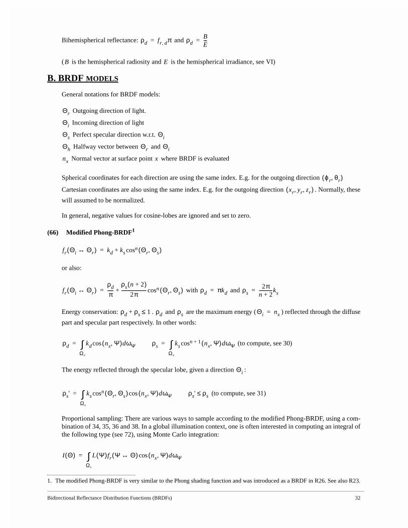
B. BRDF MODELS

General notations for BRDF models:

Outgoing direction of light.

Incoming direction of light

Perfect specular direction w.r.t.

Halfway vector between and

Normal vector at surface point where BRDF is evaluated

Spherical coordinates for each direction are using the same index. E.g. for the outgoing direction

Cartesian coordinates are also using the same index. E.g. for the outgoing direction . Normally, these

will assumed to be normalized.

In general, negative values for cosine-lobes are ignored and set to zero.

(66) Modified Phong-BRDF1

or also:

with and

Energy conservation: . and are the maximum energy ( ) reflected through the diffuse

part and specular part respectively. In other words:

(to compute, see 30)

The energy reflected through the specular lobe, given a direction :

(to compute, see 31)

Proportional sampling: There are various ways to sample according to the modified Phong-BRDF, using a com-bination of 34, 35, 36 and 38. In a global illumination context, one is often interested in computing an integral ofthe following type (see 72), using Monte Carlo integration:

1. The modified Phong-BRDF is very similar to the Phong shading function and was introduced as a BRDF in R26. See also R23.

ρd fr d, π= ρdBE---=

B E

Θr

Θi

Θs Θi

Θh Θr Θi

nx x

ϕr θr,( )

xr yr zr, ,( )

fr Θi Θr↔( ) kd ks Θr Θs,( )cosn+=

fr Θi Θr↔( )ρd

π-----

ρs n 2+( )2π

---------------------- Θr Θs,( )cosn+= ρd πkd= ρs2π

n 2+------------ks=

ρd ρs+ 1≤ ρd ρs Θi nx=

ρd kd nx Ψ,( )dωΨcos

Ωx

∫= ρs ks nx Ψ,( )dωΨcosn 1+

Ωx

∫=

Θi

ρs' ks Θr Θs,( )cosn nx Ψ,( )dωΨcos

Ωx

∫= ρs' ρs≤

I Θ( ) L Ψ( )fr Ψ Θ↔( ) nx Ψ,( )dωΨcos

Ωx

∫=

Bidirectional Reflectance Distribution Functions (BRDFs) 33

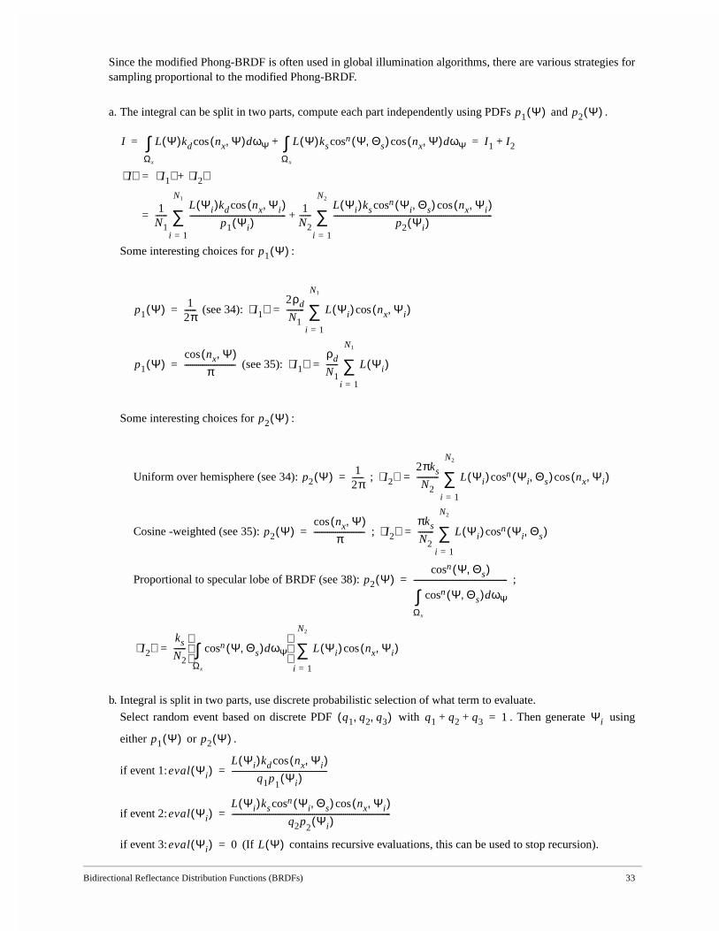
Since the modified Phong-BRDF is often used in global illumination algorithms, there are various strategies forsampling proportional to the modified Phong-BRDF.

a. The integral can be split in two parts, compute each part independently using PDFs and .

Some interesting choices for :

(see 34):

(see 35):

Some interesting choices for :

Uniform over hemisphere (see 34): ;

Cosine -weighted (see 35): ;

Proportional to specular lobe of BRDF (see 38): ;

b. Integral is split in two parts, use discrete probabilistic selection of what term to evaluate.

Select random event based on discrete PDF with . Then generate using

either or .

if event 1:

if event 2:

if event 3: (If contains recursive evaluations, this can be used to stop recursion).

p1 Ψ( ) p2 Ψ( )

I L Ψ( )kd nx Ψ,( )dωΨcos

Ωx

∫ L Ψ( )ks Ψ Θs,( )cosn nx Ψ,( )dωΨcos

Ωx

∫+ I1 I2+= =

I⟨ ⟩ I1⟨ ⟩ I2⟨ ⟩+=

1N1------

L Ψi( )kd nx Ψi,( )cos

p1 Ψi( )-------------------------------------------------

i 1=

N1

∑ 1N2------

L Ψi( )ks Ψi Θs,( )cosn nx Ψi,( )cos

p2 Ψi( )---------------------------------------------------------------------------------

i 1=

N2

∑+=

p1 Ψ( )

p1 Ψ( ) 12π------= I1⟨ ⟩

2ρd

N1--------- L Ψi( ) nx Ψi,( )cos

i 1=

N1

∑=

p1 Ψ( )nx Ψ,( )cos

π--------------------------= I1⟨ ⟩

ρd

N1------ L Ψi( )

i 1=

N1

∑=

p2 Ψ( )

p2 Ψ( ) 12π------= I2⟨ ⟩

2πks

N2----------- L Ψi( ) Ψi Θs,( )cosn nx Ψi,( )cos

i 1=

N2

∑=

p2 Ψ( )nx Ψ,( )cos

π--------------------------= I2⟨ ⟩

πks

N2-------- L Ψi( ) Ψi Θs,( )cosn

i 1=

N2

∑=

p2 Ψ( )Ψ Θs,( )cosn

Ψ Θs,( )cosn dωΨΩx

∫------------------------------------------------=

I2⟨ ⟩ks

N2------ Ψ Θs,( )cosn dωΨ

Ωx

∫

L Ψi( ) nx Ψi,( )cos

i 1=

N2

∑=

q1 q2 q3, ,( ) q1 q2 q3+ + 1= Ψi

p1 Ψ( ) p2 Ψ( )

eval Ψi( )L Ψi( )kd nx Ψi,( )cos

q1p1

Ψi( )-------------------------------------------------=

eval Ψi( )L Ψi( )ks Ψi Θs,( )cosn nx Ψi,( )cos

q2p2

Ψi( )---------------------------------------------------------------------------------=

eval Ψi( ) 0= L Ψ( )

Bidirectional Reflectance Distribution Functions (BRDFs) 34

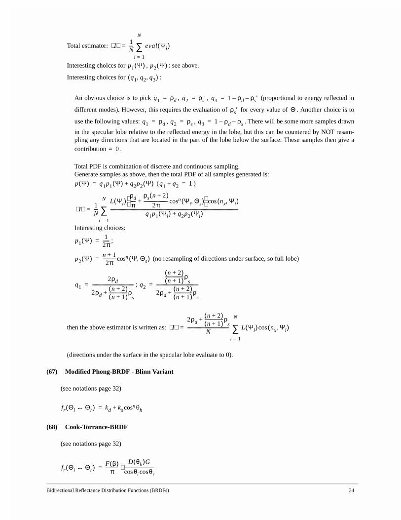
Total estimator:

Interesting choices for , : see above.

Interesting choices for :

An obvious choice is to pick , , (proportional to energy reflected in

different modes). However, this requires the evaluation of for every value of . Another choice is to

use the following values: , , . There will be some more samples drawn

in the specular lobe relative to the reflected energy in the lobe, but this can be countered by NOT resam-pling any directions that are located in the part of the lobe below the surface. These samples then give acontribution .

Total PDF is combination of discrete and continuous sampling.Generate samples as above, then the total PDF of all samples generated is:

( )

Interesting choices:

;

(no resampling of directions under surface, so full lobe)

;

then the above estimator is written as:

(directions under the surface in the specular lobe evaluate to 0).

(67) Modified Phong-BRDF - Blinn Variant

(see notations page 32)

(68) Cook-Torrance-BRDF

(see notations page 32)

I⟨ ⟩ 1N---- eval Ψi( )

i 1=

N

∑=

p1 Ψ( ) p2 Ψ( )

q1 q2 q3, ,( )

q1 ρd= q2 ρs'= q3 1 ρd– ρs'–=

ρs' Θ

q1 ρd= q2 ρs= q3 1 ρd ρs––=

0=

p Ψ( ) q1p1 Ψ( ) q2p2 Ψ( )+= q1 q2+ 1=

I⟨ ⟩ 1N----

L Ψi( )ρd

π-----

ρs n 2+( )2π

---------------------- Ψi Θs,( )cosn+ nx Ψi,( )cos

q1p1 Ψi( ) q2p2 Ψi( )+---------------------------------------------------------------------------------------------------------------------

i 1=

N

∑=

p1 Ψ( ) 12π------=

p2 Ψ( ) n 1+2π

------------ Ψ Θs,( )cosn=

q1

2ρd

2ρdn 2+( )n 1+( )

-----------------ρs

+--------------------------------------= q2

n 2+( )n 1+( )

-----------------ρs

2ρdn 2+( )n 1+( )

-----------------ρs

+--------------------------------------=

I⟨ ⟩2ρd

n 2+( )n 1+( )

-----------------ρs

+

N-------------------------------------- L Ψi( ) nx Ψi,( )cos

i 1=

N

∑=

fr Θi Θr↔( ) kd ks θhcosn+=

fr Θi Θr↔( ) F β( )π

------------D θh( )G

θi θrcoscos----------------------------⋅=

Bidirectional Reflectance Distribution Functions (BRDFs) 35

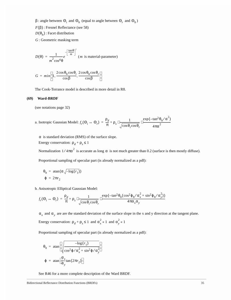
: angle between and (equal to angle between and )

: Fresnel Reflectance (see 58)

: Facet distribution

: Geometric masking term

( is material-parameter)

The Cook-Torrance model is described in more detail in R8.

(69) Ward-BRDF

(see notations page 32)

a. Isotropic Gaussian Model:

is standard deviation (RMS) of the surface slope.

Energy conservation:

Normalization is accurate as long is not much greater than 0.2 (surface is then mostly diffuse).

Proportional sampling of specular part (is already normalized as a pdf):

b. Anisotropic Elliptical Gaussian Model:

and are are the standard deviation of the surface slope in the x and y direction at the tangent plane.

Energy conservation: and and

Proportional sampling of specular part (is already normalized as a pdf):

See R46 for a more complete description of the Ward BRDF.

β Θi Θh Θr Θh

F β( )D θh( )

G

D θ( ) 1

m2 θcos4

---------------------e

θtanm

-----------2

–

= m

G min 12 θh θicoscos

βcos--------------------------------

2 θh θrcoscos

βcos--------------------------------, ,

=

fr Θi Θr↔( )ρd

π----- ρs

1

θi θrcoscos--------------------------------

θhtan2 α2⁄–( )exp

4πα2--------------------------------------------⋅ ⋅+=

αρd ρs+ 1≤

1 4πα2⁄ α

θh α r1( )log–( )atan=

ϕ 2πr2=

fr Θi Θr↔( )ρd

π----- ρs

1

θi θrcoscos--------------------------------

θhtan2 ϕhcos2 αx2⁄ ϕhsin2 αy

2⁄+( )–( )exp

4παxαy----------------------------------------------------------------------------------------------------⋅ ⋅+=

αx αy

ρd ρs+ 1≤ αx2

1« αy2

1«

θh

r1( )log–

ϕcos2 αx2⁄ ϕsin2 αy

2⁄+--------------------------------------------------------

atan=

ϕαx

αy------ 2πr2( )tan

atan=

Bidirectional Reflectance Distribution Functions (BRDFs) 36

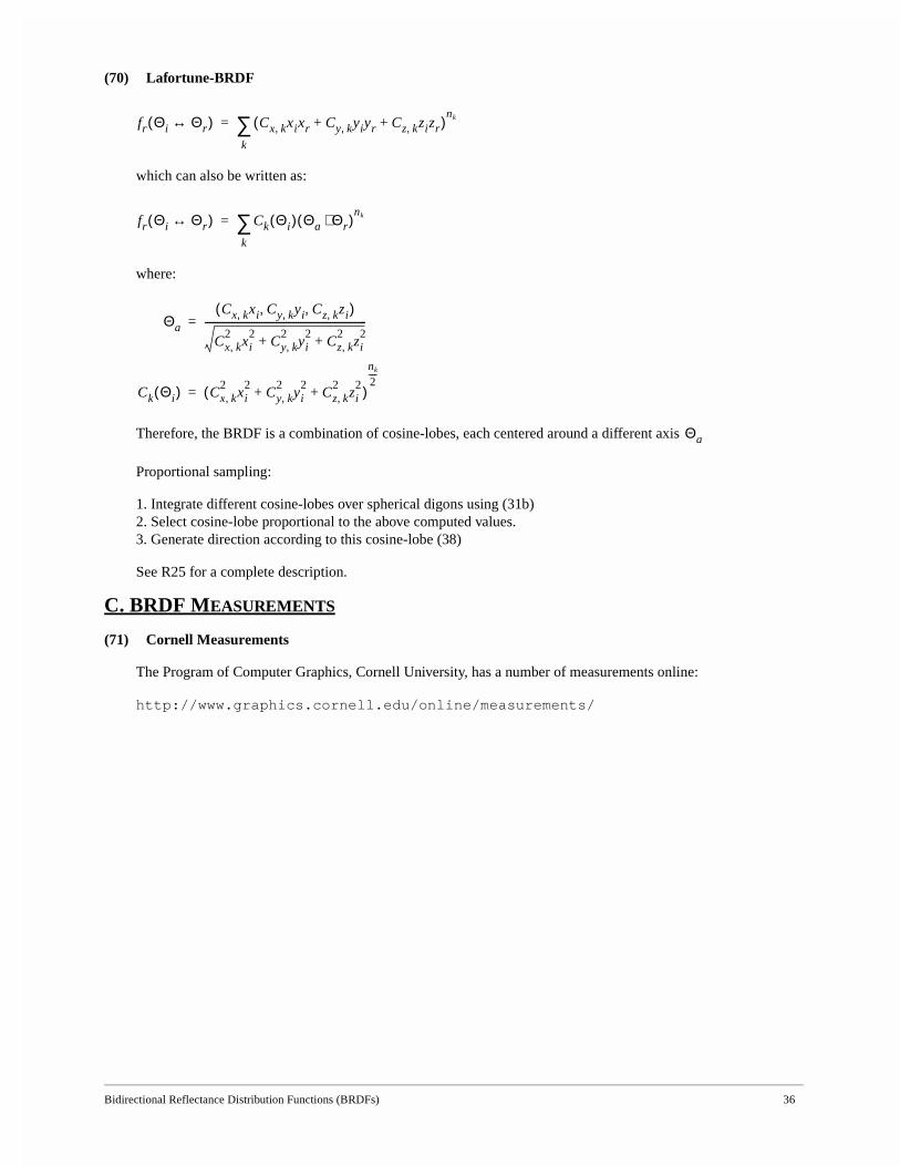
(70) Lafortune-BRDF

which can also be written as:

where:

Therefore, the BRDF is a combination of cosine-lobes, each centered around a different axis

Proportional sampling:

1. Integrate different cosine-lobes over spherical digons using (31b)2. Select cosine-lobe proportional to the above computed values.3. Generate direction according to this cosine-lobe (38)

See R25 for a complete description.

C. BRDF MEASUREMENTS

(71) Cornell Measurements

The Program of Computer Graphics, Cornell University, has a number of measurements online:

http://www.graphics.cornell.edu/online/measurements/

fr Θi Θr↔( ) Cx k, xixr Cy k, yiyr Cz k, zizr+ +( )nk

k

∑=

fr Θi Θr↔( ) Ck Θi( ) Θa Θr⋅( )nk

k

∑=

Θa

Cx k, xi Cy k, yi Cz k, zi, ,( )

Cx k,2

xi2

Cy k,2

yi2

Cz k,2

zi2

+ +------------------------------------------------------------------=

Ck Θi( ) Cx k,2

xi2

Cy k,2

yi2

Cz k,2

zi2

+ +( )

nk

2----

=

Θa

Rendering Equation and Global Illumination Formulations 37

IX. Rendering Equation and Global Illumination Formulations

A. RADIANCE TRANSPORT FORMULATIONS

All formulations in this section take radiance as the main transport quantity. For the sake of clarity, the wavelengthdependency of radiance values is implicitly assumed in all equations.

(72) Rendering Equation (Radiance), integration over incoming hemisphere

Direct illumination only:

(73) Rendering Equation (Radiance), integration over all surfaces in the scene

(many authors include in the definition of , but in this document they are kept separate forclarity).

Direct illumination only: see 74.

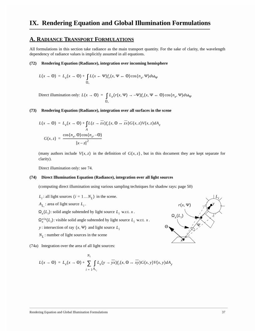
(74) Direct Illumination Equation (Radiance), integration over all light sources

(computing direct illumination using various sampling techniques for shadow rays: page 50)

: all light sources in the scene.

: area of light source .

: solid angle subtended by light source w.r.t. .

: visible solid angle subtended by light source w.r.t. .

: intersection of ray and light source

: number of light sources in the scene

(74a) Integration over the area of all light sources:

L x Θ→( ) Le x Θ→( ) L x Ψ←( )fr x Ψ Θ↔,( ) nx Ψ,( )dωΨcos

Ωx

∫+=

L x Θ→( ) Le r x Ψ,( ) Ψ–→( )fr x Ψ Θ↔,( ) nx Ψ,( )dωΨcos

Ωx

∫=

L x Θ→( ) Le x Θ→( ) L z zx→( )fr x Θ zx↔,( )G x z,( )V x z,( )dAz

A

∫+=

G x z,( )nx Θ,( ) nz Θ–,( )coscos

x z–2

--------------------------------------------------------=

V x z,( ) G x z,( )

x

Li

Θ

y

Ωx Li( )

Ψ

r x Ψ,( )

Li i 1…NL=( )

ALiLi

Ωx Li( ) Li x

Ωxvis Li( ) Li x

y x Ψ,( ) Li

NL

L x Θ→( ) Le x Θ→( ) Le y yx→( )fr x Θ xy↔,( )G x y,( )V x y,( )dAy

ALi

∫i 1=

NL

∑+=

Rendering Equation and Global Illumination Formulations 38

(74b) Integration over solid angles subtended by light sources:

(74c) Integration over visible solid angles subtended by light sources:

(in this case )

(75) Continuous Radiosity Equation: diffuse reflection, diffuse light sources, integration over surfaces

If all surfaces are diffuse reflectors and light sources are diffuse emitters, radiance values are independent ofdirection and can be expressed by the hemispherical radiometric quantities:

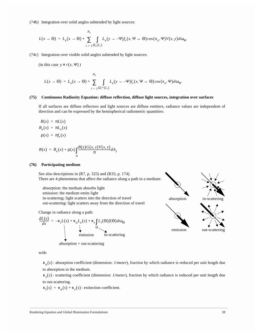
(76) Participating medium

See also descriptions in (R7, p. 325) and (R33, p. 174).There are 4 phenomena that affect the radiance along a path in a medium:

absorption: the medium absorbs lightemission: the medium emits lightin-scattering: light scatters into the direction of travelout-scattering: light scatters away from the direction of travel

Change in radiance along a path:

with:

: absorption coefficient (dimension: 1/meter), fraction by which radiance is reduced per unit length due

to absorption in the medium.: scattering coefficient (dimension: 1/meter), fraction by which radiance is reduced per unit length due

to out-scattering.: extinction coefficient.

L x Θ→( ) Le x Θ→( ) Le y Ψ–→( )fr x Ψ Θ↔,( ) nx Ψ,( )V x y,( )dωΨcos

Ωx Li( )∫

i 1=

NL

∑+=

y r x Ψ,( )≡

L x Θ→( ) Le x Θ→( ) Le y Ψ–→( )fr x Ψ Θ↔,( ) nx Ψ,( )dωΨcos

Ωxvis Li( )∫

i 1=

NL

∑+=

B x( ) πL x( )=

Be x( ) πLe x( )=

ρ x( ) πfr x( )=

B x( ) Be x( ) ρ x( ) B z( )G x z,( )V x z,( )π

----------------------------------------------dAz

A

∫+=

absorption in-scattering

emission out-scattering

dL s( )ds

-------------- κ– tL s( ) κaLe s( ) κs Li Θ( )f Θ( )dωΘΩ∫+ +=

absorption + out-scattering

emission in-scattering

κa s( )

κs s( )

κ t s( ) κa s( ) κs s( )+=

Rendering Equation and Global Illumination Formulations 39

: phase function, describing fraction of radiance arriving from direction that is in-scattered along the

path. If the medium is isotropic:

Solving the above differential equation:

with:

: transmittance function. If the medium is isotropic, is constant and thus

: source function, describing in-scattering and emission.

: scattering albedo of the medium

(77) Participating medium, no scattering

Equations in 76 apply, with and

and if and constant:

(can be used as a simple fog-model)

B. DUAL TRANSPORT FORMULATION

Light transport can also be formulated by using the adjoint equations. The adjoint transport quantity is called impor-

tance or potential function by various authors, and an often used notation is . An intuitive way of thinking about thepotential function is to consider it an incident function in combination with radiance as an exitant function.

(78) Relationship between Flux, Radiance, Potential

See R12 for a more complete description.

Consider a set of surface points and associated directions . The exitant flux for can

be written as:

f Θ( ) Θ

fisotropic1

4π------=

L s( ) L 0( )τ 0 s,( ) τ s' s,( )J s'( )κ t s'( ) s'd

0

s

∫+=

τ s1 s2,( ) κ t s( ) sd

s1

s2

∫–

exp= κ t s( )

τ s1 s2,( ) eκ– t s1 s2–

=

J s( )

J s( ) 1 R s( )–( )Le s( ) R s( ) Li Θ( )f Θ( )dωΘΩ∫+=

R s( )κs s( )κ t s( )------------

κs s( )κa s( ) κs s( )+--------------------------------= =

κs s( ) 0= κa s( ) κ t s( )=

L s( ) L 0( )τ 0 s,( ) Le s'( )τ s' s,( )κ t s'( ) s'd

0

s

∫+=

κ t s( ) Le s( )

L s( ) L 0( )eκ– t s Le 1 e

κ– t s–( )+=

W

S S As Ωx× A Ω×⊂= S

Rendering Equation and Global Illumination Formulations 40

with the initial potential, defined as:

The above integral can also be formally defined as an inner product: .

Using the dual formulation, can also be written as an integral over all light sources, or formally:

with

is dimensionless and has the same transport properties as radiance (invariant along straight lines).

Φ S( ) L x Θ→( )We x Θ←( ) Θ nx,( )cos ωΘd Axd

Ω∫

A

∫=

We x Θ←( )

We x Θ←( )1 if x Θ,( ) S∈0 if x Θ,( ) S∉

=

Φ S( ) L We,⟨ ⟩=

Φ S( )

Φ S( ) Le x Θ→( )W x Θ←( ) Θ nx,( )cos ωΘd Axd

Ω∫

A

∫ Le W,⟨ ⟩= =

W x Θ←( ) We x Θ←( ) W r x Θ,( ) Ψ←( )fr r x Θ,( ) Ψ Θ↔,( ) nr x Θ,( ) Ψ,( )dωΨcos

Ωr x Θ,( )

∫+=

W x Θ←( )

Form Factors 41

X. Form Factors

Form Factor: the fraction of uniform diffuse radiant energy leaving one surface that is incident upon a second sur-face.

Form Factor Algebra: mathematical relations between form factors

Notation: The ‘sender’ surface is written as the first index, the ‘receiver’ surface as the second. An arrow indicates the‘energy flow’. This notation is consistent with other notations in literature, where the arrow usually is not used.

Form Factors are usually treated very extensively in books dealing with thermal radiation heat transfer (R32).

A good on-line resource for analytical avaluations of form factors: “A Catalog of Radiation Heat Transfer Configura-tion Factors” by John R. Howell: http://www.me.utexas.edu/~howell/

Global illumination context: computing form factors is one of the main elements of radiosity algorithms. Radiosityalgorithms based on some variant of particle tracing often implicitly compute form factors without storing them.Direct illumination computations in ray tracing using shadow-rays also often implicitly computes a point-to-area formfactor.

A. GENERAL EXPRESSIONS AND PROPERTIES

(79) Differential element to differential element Form Factor

With visibility term:

(80) Differential element to element Form Factor

(81) Differential element to polygon Form Factor; full visibility

( = number of edges or vertices of the polygon)

where and magnitude of .

See also R3.

nx

ny

x

y

dAy

dAx

rxyθx

θydFdAx dAy→θx θycoscos

πrxy2

-----------------------------dAyG x y,( )

π-----------------dAy= =

dFdAx dAy→θx θycoscos

πrxy2

-----------------------------V x y,( )dAyG x y,( )V x y,( )

π-----------------------------------dAy= =

FdAx j→θx θycoscos

πrxy2

-----------------------------V x y,( )dAy

Aj

∫ G x y,( )V x y,( )π

-----------------------------------dAy

Aj

∫= =

nx γi

Vi

Vi 1+

dAx

FdAx j→1

2π------ nx Γ i⋅

i 1=

E

∑= E

Γ i Vi Vi 1+⊗= Γ i γi=

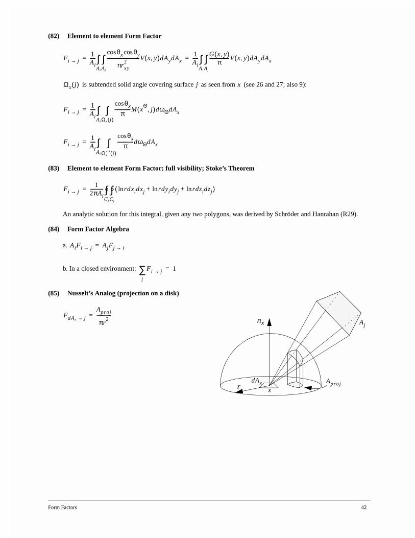
Form Factors 42

(82) Element to element Form Factor

is subtended solid angle covering surface as seen from (see 26 and 27; also 9):

(83) Element to element Form Factor; full visibility; Stoke’s Theorem

An analytic solution for this integral, given any two polygons, was derived by Schröder and Hanrahan (R29).

(84) Form Factor Algebra

a.

b. In a closed environment:

(85) Nusselt’s Analog (projection on a disk)

Fi j→1Ai-----

θx θycoscos

πrxy2

-----------------------------V x y,( )dAydAx

Aj

∫Ai

∫ 1Ai----- G x y,( )

π-----------------V x y,( )dAydAx

Aj

∫Ai

∫= =

Ωx j( ) j x

Fi j→1Ai-----

θxcos

π--------------M x

Θj,( )dωΘdAx

Ωx j( )∫

Ai

∫=

Fi j→1Ai-----

θxcos

π--------------dωΘdAx

Ωxvis j( )

∫Ai

∫=

Fi j→1

2πAi------------ rdxidxjln rdyidyjln rdzidzjln+ +( )

Cj

∫°Ci

∫°=

AiFi j→ AjFj i→=

Fi j→j

∑ 1=

nx

rdAx

Aj

Aprojx

FdAx j→Aproj

πr2

-------------=

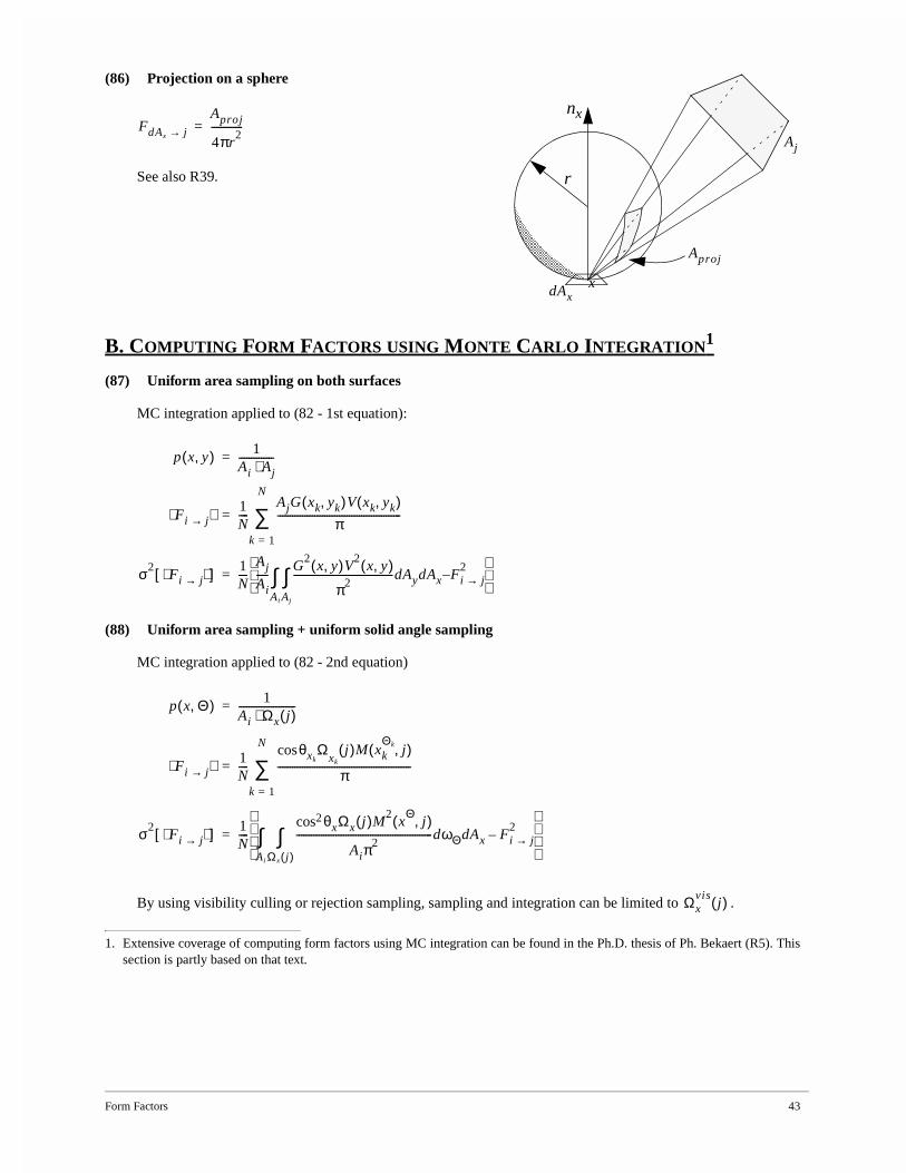
Form Factors 43

(86) Projection on a sphere

See also R39.

B. COMPUTING FORM FACTORS USING MONTE CARLO INTEGRATION1

(87) Uniform area sampling on both surfaces

MC integration applied to (82 - 1st equation):

(88) Uniform area sampling + uniform solid angle sampling

MC integration applied to (82 - 2nd equation)

By using visibility culling or rejection sampling, sampling and integration can be limited to .

1. Extensive coverage of computing form factors using MC integration can be found in the Ph.D. thesis of Ph. Bekaert (R5). Thissection is partly based on that text.

nx

r

dAx

Aj

Aproj

x

FdAx j→Aproj

4πr2

-------------=

p x y,( ) 1Ai Aj⋅--------------=

Fi j→⟨ ⟩ 1N----

AjG xk yk,( )V xk yk,( )π

--------------------------------------------------

k 1=

N

∑=

σ2Fi j→⟨ ⟩[ ] 1

N----

Aj

Ai-----

G2

x y,( )V2

x y,( )

π2----------------------------------------dAydAx

Aj

∫Ai

∫ Fi j→2

–

=

p x Θ,( ) 1Ai Ωx j( )⋅-----------------------=

Fi j→⟨ ⟩ 1N----

θxkcos Ω

xkj( )M xk

Θk j,( )

π------------------------------------------------------

k 1=

N

∑=

σ2Fi j→⟨ ⟩[ ] 1

N----

θxcos2 Ωx j( )M2

xΘ

j,( )

Aiπ2

-------------------------------------------------------dωΘdAx

Ωx j( )∫

Ai

∫ Fi j→2

–

=

Ωxvis

j( )

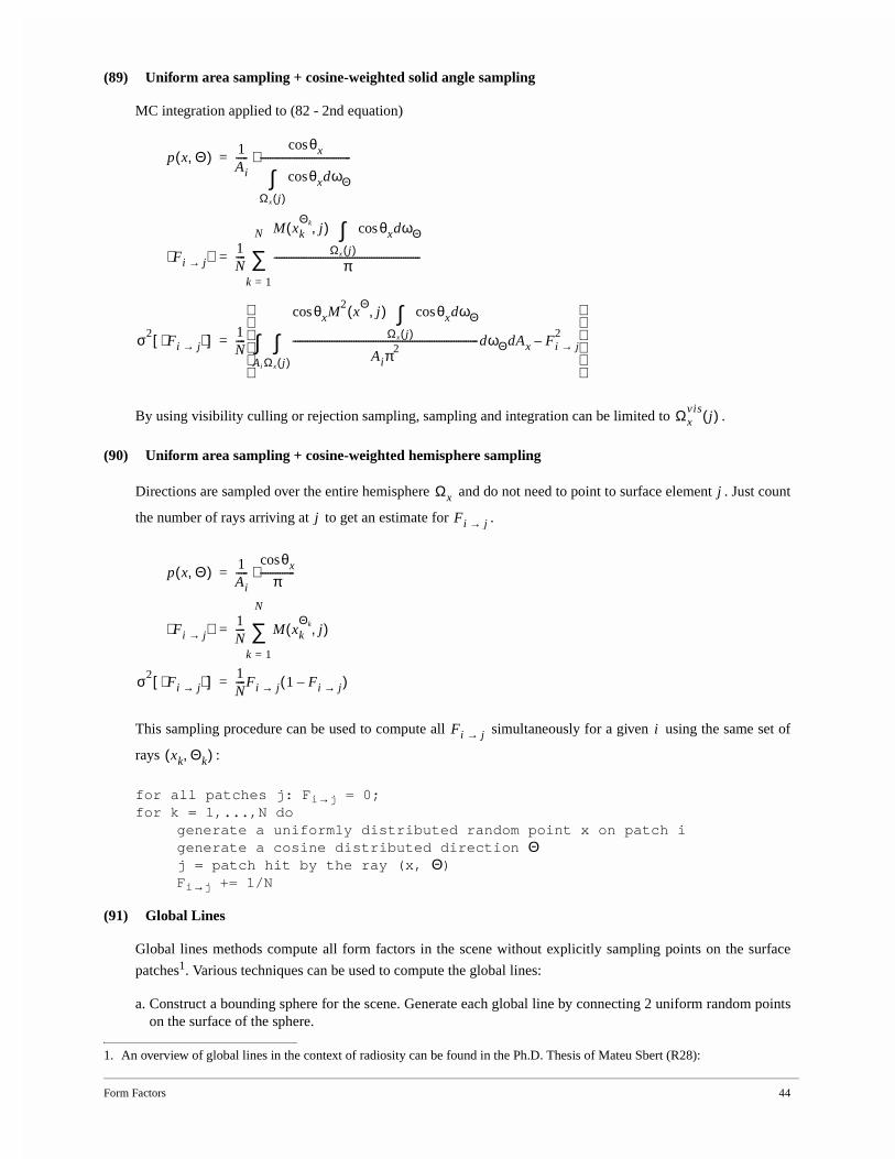
Form Factors 44

(89) Uniform area sampling + cosine-weighted solid angle sampling

MC integration applied to (82 - 2nd equation)

By using visibility culling or rejection sampling, sampling and integration can be limited to .

(90) Uniform area sampling + cosine-weighted hemisphere sampling

Directions are sampled over the entire hemisphere and do not need to point to surface element . Just count

the number of rays arriving at to get an estimate for .

This sampling procedure can be used to compute all simultaneously for a given using the same set of

rays :

for all patches j: Fi→j = 0;for k = 1,...,N do

generate a uniformly distributed random point x on patch igenerate a cosine distributed direction Θj = patch hit by the ray (x, Θ)Fi→j += 1/N

(91) Global Lines

Global lines methods compute all form factors in the scene without explicitly sampling points on the surface

patches1. Various techniques can be used to compute the global lines:

a. Construct a bounding sphere for the scene. Generate each global line by connecting 2 uniform random pointson the surface of the sphere.

1. An overview of global lines in the context of radiosity can be found in the Ph.D. Thesis of Mateu Sbert (R28):

p x Θ,( ) 1Ai-----

θxcos

θxcos dωΘΩx j( )∫

-------------------------------------⋅=

Fi j→⟨ ⟩ 1N----

M xkΘk j,( ) θxcos dωΘ

Ωx j( )∫π

------------------------------------------------------------

k 1=

N

∑=

σ2Fi j→⟨ ⟩[ ] 1

N----

θxcos M2

xΘ

j,( ) θxcos dωΘΩx j( )∫

Aiπ2

----------------------------------------------------------------------------dωΘdAx

Ωx j( )∫

Ai

∫ Fi j→2

–

=

Ωxvis

j( )

Ωx j

j Fi j→

p x Θ,( ) 1Ai-----

θxcos

π--------------⋅=

Fi j→⟨ ⟩ 1N---- M xk

Θk j,( )

k 1=

N

∑=

σ2Fi j→⟨ ⟩[ ] 1

N----Fi j→ 1 Fi j→–( )=

Fi j→ i

xk Θk,( )

Form Factors 45

b. Generate a random direction on the unit sphere. Project the scene on a plane perpendicular to . Generate

a uniformly distributed random surface point in the projection. is a global line.

All global lines are intersected with all surfaces in the scene, resulting in several spans on each line. The proba-bility that a line intersects a surface is proportional to the area of that surface.

is estimated by , with the number of spans connecting surface patches and , and the

number of spans starting from surface patch .

Θ Θx x Θ,( )

Fi j→ Nij Ni⁄ Nij i j Ni

i

Radiosity System & Algorithms 46

XI. Radiosity System & Algorithms

The term ‘Radiosity’ is used in various ways in photorealistic image synthesis: as the radiometric quantity describingincident energy integrated over the hemisphere; but also to indicate a specific class of algorithms that compute anenergy distribution in the scene. Although there is no formal definition of what a ‘radiosity algorithm’ actually is, it isusually assumed that one means a finite-element solution, computing diffuse light interaction only.

Most radiosity literature uses Galerkin Radiosity, a projection method to transform the continuous radiosity equations(75) into a set of linear equations. Unless otherwise indicated, Galerkin radiosity is used in this section.

Notations:

: constant radiosity of patch i (see 49, 51) - expressed in Watt/m2

: self-emitted constant radiosity of patch i - expressed in Watt/m2

: diffuse bihemispherical reflectance of patch i (see 65) - dimensionless

: form factor between patch i and j (see 82) - dimensionless

: power of patch i - expressed in Watt

: surface area of patch i - expressed in m2

(92) System of radiosity equations, constant basis functions

(93) System of power equations, constant basis functions

(94) Discretizing the continuous radiosity equation1

Continuous radiosity equation (see 75):

1. Based on chapter 3 of R7.

Bi

Bei

ρi

Fi j→

Pi Pi AiBi=

Ai

patches i:∀ Bi Bei ρi Fi j→ Bj

j

∑+=

1 ρ1F1 1→– ρ1F1 2→– … ρ1F1 n→–

ρ2F2 1→– 1 ρ2F2 2→– … ρ2F2 n→–

… … … …ρnFn 1→– ρnFn 2→– … 1 ρnFn n→–

B1

B2

…Bn

Be1

Be2

…Ben

=

patches i:∀ Pi Pei ρi Fj i→ Pj

j

∑+=

1 ρ1F1 1→– ρ1F2 1→– … ρ1Fn 1→–

ρ2F1 2→– 1 ρ2F2 2→– … ρ2Fn 2→–

… … … …ρnF1 n→– ρnF2 n→– … 1 ρnFn n→–

P1

P2

…Pn

Pe1

Pe2

…Pen

=

B x( ) Be x( ) ρ x( ) B z( )G x z,( )V x z,( )π

----------------------------------------------dAz

A

∫+=

Radiosity System & Algorithms 47

Approximation of :

Residual (substitute in continuous equation):

General approach: pick weighting functions . The norm of residual: .

Each of the terms can now be set to be zero, resulting in a linear equation for

each .

(94a) Point Collocation

(residual is zero for selected number of points )

then: with

(94b) Galerkin

then:

with

Choosing results in the classic radiosity formulation (92 or 93).

(95) Basic Relaxation Algorithm1

Most radiosity algorithms are relaxation methods, that solve the radiosity system through a series of iterations.This item describes the basic principle of all relaxation algorithms.

Linear system to solve: or

Subsequent iterations:

1. A very good overview of different relaxation techniques for solving the radiosity system can be found in the Ph.D. thesis ofPhilippe Bekaert (R5).

B x( ) B x( ) B x( )≈ BiNi x( )

i 1=

N

∑=

B x( ) r x( ) B x( ) Be x( ) ρ x( ) B z( )G x z,( )V x z,( )π

----------------------------------------------dAz

A

∫––=

N Wi x( ) r x( ) r x( ) Wi x( ),⟨ ⟩

i 1=

N

∑=

r x( ) Wi x( ),⟨ ⟩ r x( )Wi x( )dAx

A

∫=

Wi x( )

Wi x( ) δ x xi–( )= xi

i: ∀ KijBj

j 1=

N

∑ Be xi( )– 0= Kij Nj xi( )ρ xi( )

π------------ Nj z( )G xi z,( )V xi z,( )dAz

A

∫–=

Wi x( ) Ni x( )=

i: ∀ KijBj

j 1=

N

∑ Be x( )Ni x( )dAx

A

∫– 0=

Kij Ni x( )Nj x( )dAx

A

∫ ρ x( )Ni x( )Nj z( )G x z,( )V x z,( )π

----------------------------------dAzdAx

A

∫A

∫–=

Ni x( )1 if x belongs to surface element i

0 otherwise

=

Ax e=

a11 … a1n

… … …an1 … ann

x1

…xn

e1

…en

=

x0( )

x1( )

x2( ) …, , ,

Radiosity System & Algorithms 48

Correction vectors :

Residu vectors (measure for error): , and therefore

Basic relaxation algorithm:

Choose initial x(0);r(0) = b - A.x(0);for k = 0, 1, ... until convergence do

compute ∆x(k) (based on x(k), r(k), other information)x(k+1) = x(k) + ∆x(k);r(k+1) = r(k) - A.∆x(k);

(96) Gauss-Seidel iteration

Each component of the solution is updated in turn:

Correction vector: (all components 0 except ).

Residu vector: (component equals 0).

Applied to (93) ( if ):

Algorithm:

for all patches j: Pj = Pej;cycle through patches until convergence (selected patch = s)

Ps = Pes;for all patches j

Ps += ρs.Fj→s.Pj;

Incremental Gauss-Seidel: compute residu vector explicitly and increment solution vector instead of replacingprevious solution.

∆xk( )

xk 1+( )

xk( ) ∆x

k( )+=

rk( )

rk( )

e Axk( )

–= rk 1+( )

rk( )

A∆xk( )

–=

xs es asjxj

j s≠∑–

ass⁄←

∆xi δisrs

ass⁄← s

ri ri aisrsass⁄–← s

ass 1= Fs s→ 1=

Ps Pes ρs Fj s→ Pj

j s≠∑+←

Radiosity Extensions 49

XII. Radiosity Extensions

(97) Clustering - Equivalent extinction coefficient

When clustering objects, an equivalent isotropic extinction coefficient can be computed for the cluster (R35), inan analogy with a participating medium (76).

where is the total surface area of objects in the cluster and is the volume of the cluster.

Directional extinction (R34):

where is the total projected area in direction .

(98) Final Gathering

A final gathering step is used to make a high-quality rendering of a radiosity solution, using a per-pixel radi-ance computation. It usually involves computing a radiance value for the visible surface point through eachpixel, using the radiosity values stored on the surface patches.

Suppose is the pre-computed (diffuse) radiosity solution, then the radiance for surface point in direction can be approximated as (see section IX for basic rendering equation):

(hemisphere integration)

or:

(surface integration)

The integral in either of the two above formulations can be approximated by an appropriate sampling technique,thereby ‘gathering’ radiance from the other surfaces. Many different variants are possible, depending on howmuch information was stored with the radiosity solution.

Variants: Uniform hemisphere sampling; cosine-weighted hemisphere sampling; uniform area sampling; areasampling proportional to solid angle; area sampling proportional to cosine weighted angle; area sampling pro-

portional to ; area sampling sampling proportional to stored (linked) form factors. See (R41, R4) for an over-view.

κ tA

4V-------=

A V

κ t Θ( ) A⊥ Θ( )V

----------------=

A⊥ Θ( ) Θ

L x Θ

L x Θ→( ) Le x Θ→( ) L x Ψ←( )fr x Ψ Θ↔,( ) nx Ψ,( )dωΨcos

Ωx

∫+=

L x Θ→( ) Le x Θ→( ) L z zx→( )fr x Θ zx↔,( )G x z,( )V x z,( )dAz

A

∫+=

L

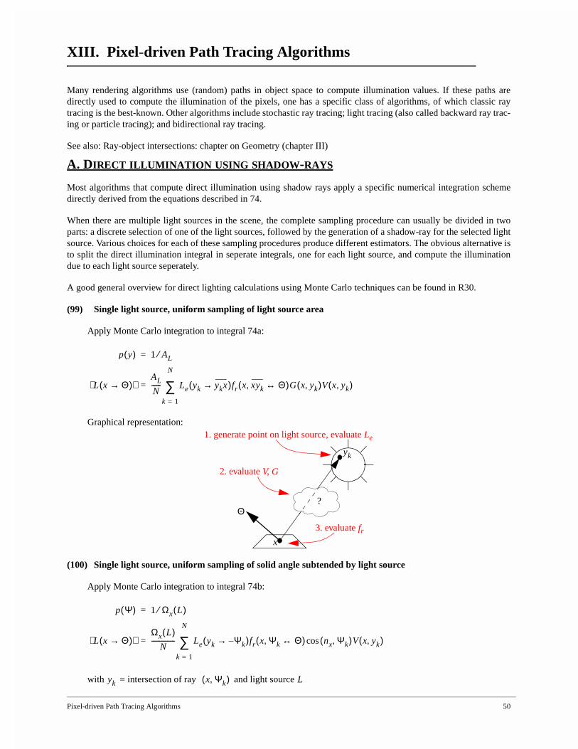
Pixel-driven Path Tracing Algorithms 50

XIII. Pixel-driven Path Tracing Algorithms

Many rendering algorithms use (random) paths in object space to compute illumination values. If these paths aredirectly used to compute the illumination of the pixels, one has a specific class of algorithms, of which classic raytracing is the best-known. Other algorithms include stochastic ray tracing; light tracing (also called backward ray trac-ing or particle tracing); and bidirectional ray tracing.

See also: Ray-object intersections: chapter on Geometry (chapter III)

A. DIRECT ILLUMINATION USING SHADOW-RAYS

Most algorithms that compute direct illumination using shadow rays apply a specific numerical integration schemedirectly derived from the equations described in 74.

When there are multiple light sources in the scene, the complete sampling procedure can usually be divided in twoparts: a discrete selection of one of the light sources, followed by the generation of a shadow-ray for the selected lightsource. Various choices for each of these sampling procedures produce different estimators. The obvious alternative isto split the direct illumination integral in seperate integrals, one for each light source, and compute the illuminationdue to each light source seperately.

A good general overview for direct lighting calculations using Monte Carlo techniques can be found in R30.

(99) Single light source, uniform sampling of light source area

Apply Monte Carlo integration to integral 74a:

Graphical representation:

(100) Single light source, uniform sampling of solid angle subtended by light source

Apply Monte Carlo integration to integral 74b:

with = intersection of ray and light source

p y( ) 1 AL⁄=

L x Θ→( )⟨ ⟩AL

N------ Le yk ykx→( )fr x xyk Θ↔,( )G x yk,( )V x yk,( )

k 1=

N

∑=

x

Θ

yk

1. generate point on light source, evaluate Le

?

2. evaluate V, G

3. evaluate fr

p Ψ( ) 1 Ωx L( )⁄=

L x Θ→( )⟨ ⟩Ωx L( )

N--------------- Le yk Ψk–→( )fr x Ψk Θ↔,( ) nx Ψk,( )V x yk,( )cos

k 1=

N

∑=

yk x Ψk,( ) L

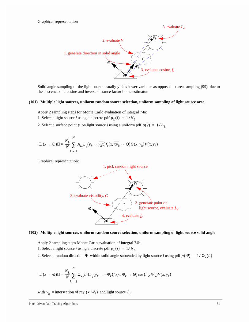
Pixel-driven Path Tracing Algorithms 51

Graphical representation

Solid angle sampling of the light source usually yields lower variance as opposed to area sampling (99), due tothe abscence of a cosine and inverse distance factor in the estimator.

(101) Multiple light sources, uniform random source selection, uniform sampling of light source area

Apply 2 sampling steps for Monte Carlo evaluation of integral 74a:

1. Select a light source i using a discrete pdf

2. Select a surface point on light source i using a uniform pdf

Graphical representation:

(102) Multiple light sources, uniform random source selection, uniform sampling of light source solid angle

Apply 2 sampling steps Monte Carlo evaluation of integral 74b:1. Select a light source i using a discrete pdf

2. Select a random direction within solid angle subtended by light source i using pdf

with = intersection of ray and light source

x

Θ

yk

1. generate direction in solid angle?

2. evaluate V

3. evaluate cosine, frΨk

3. evaluate Le

pL i( ) 1 NL⁄=

y p y( ) 1 ALi⁄=

L x Θ→( )⟨ ⟩NL

N------ ALk

Le

yk ykx→( )fr x xyk Θ↔,( )G x yk,( )V x yk,( )

k 1=

N

∑=

x

Θ

yk

2. generate point on?

3. evaluate visibility, G

4. evaluate fr

light source, evaluate Le

1. pick random light source

pL i( ) 1 NL⁄=

Ψ p Ψ( ) 1 Ωx L( )⁄=

L x Θ→( )⟨ ⟩NL

N------ Ωx Li( )L

eyk Ψk–→( )fr x Ψk Θ↔,( ) nx Ψk,( )V x yk,( )cos

k 1=

N

∑=

yk x Ψk,( ) Li

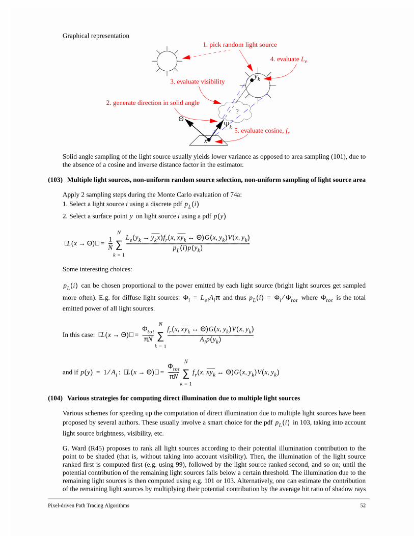
Pixel-driven Path Tracing Algorithms 52

Graphical representation

Solid angle sampling of the light source usually yields lower variance as opposed to area sampling (101), due tothe absence of a cosine and inverse distance factor in the estimator.

(103) Multiple light sources, non-uniform random source selection, non-uniform sampling of light source area

Apply 2 sampling steps during the Monte Carlo evaluation of 74a:1. Select a light source i using a discrete pdf

2. Select a surface point on light source i using a pdf

Some interesting choices:

can be chosen proportional to the power emitted by each light source (bright light sources get sampled

more often). E.g. for diffuse light sources: and thus where is the total

emitted power of all light sources.

In this case:

and if :

(104) Various strategies for computing direct illumination due to multiple light sources

Various schemes for speeding up the computation of direct illumination due to multiple light sources have beenproposed by several authors. These usually involve a smart choice for the pdf in 103, taking into account

light source brightness, visibility, etc.

G. Ward (R45) proposes to rank all light sources according to their potential illumination contribution to thepoint to be shaded (that is, without taking into account visibility). Then, the illumination of the light sourceranked first is computed first (e.g. using 99), followed by the light source ranked second, and so on; until thepotential contribution of the remaining light sources falls below a certain threshold. The illumination due to theremaining light sources is then computed using e.g. 101 or 103. Alternatively, one can estimate the contributionof the remaining light sources by multiplying their potential contribution by the average hit ratio of shadow rays

x

Θ

yk

2. generate direction in solid angle?

3. evaluate visibility

5. evaluate cosine, frΨk

4. evaluate Le

1. pick random light source

pL i( )

y p y( )

L x Θ→( )⟨ ⟩ 1N----

Le yk ykx→( )fr x xyk Θ↔,( )G x yk,( )V x yk,( )pL i( )p yk( )

--------------------------------------------------------------------------------------------------------------

k 1=

N

∑=

pL i( )

Φi LeiAiπ= pL i( ) Φi Φtot⁄= Φtot

L x Θ→( )⟨ ⟩Φtot

πN----------

fr x xyk Θ↔,( )G x yk,( )V x yk,( )Aip yk( )

----------------------------------------------------------------------------

k 1=

N

∑=

p y( ) 1 Ai⁄= L x Θ→( )⟨ ⟩Φtot

πN---------- fr x xyk Θ↔,( )G x yk,( )V x yk,( )

k 1=

N

∑=

pL i( )

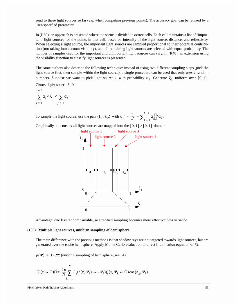
Pixel-driven Path Tracing Algorithms 53

send to these light sources so far (e.g. when computing previous points). The accuracy goal can be relaxed by auser-specified parameter.

In (R30), an approach is presented where the scene is divided in octree cells. Each cell maintains a list of ‘impor-tant’ light sources for the points in that cell, based on intensity of the light source, distance, and reflectivity.When selecting a light source, the important light sources are sampled proportional to their potential contribu-tion (not taking into account visibility), and all remaining light sources are selected with equal probability. Thenumber of samples used for the important and unimportant light sources can vary. In (R48), an extension usingthe visibility function to classify light sources is presented.

The same authors also describe the following technique: instead of using two different sampling steps (pick thelight source first, then sample within the light source), a single procedure can be used that only uses 2 random

numbers. Suppose we want to pick light source with probability . Generate uniform over .

Choose light source if:

To sample the light source, use the pair with .

Graphically, this means all light sources are mapped into the domain:

Advantage: one less random variable, so stratified sampling becomes more effective; less variance.

(105) Multiple light sources, uniform sampling of hemisphere

The main difference with the previous methods is that shadow rays are not targeted towards light sources, but aregenerated over the entire hemisphere. Apply Monte Carlo evaluation to direct illumination equation of 72.

(uniform sampling of hemisphere, see 34)

i α i ξ1 0 1,[ ]

i

α j

j 1=

i 1–

∑ ξ1 α j

j 1=

i

∑< <

ξ1' ξ2,( ) ξ1' ξ1 α jj 1=

i 1–

∑– α i⁄=

0 1,[ ] 0 1,[ ]×

ξ1

ξ2

0 10

1

α1 α2 α3 α4

light source 1

light source 4

light source 3

light source 2

0 1

ξ1'

p Ψ( ) 1 2π⁄=

L x Θ→( )⟨ ⟩ 2πN------ Le r x Ψk,( ) Ψk–→( )fr x Ψk Θ↔,( ) nx Ψk,( )cos

k 1=

N

∑=

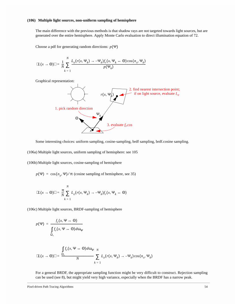
Pixel-driven Path Tracing Algorithms 54

(106) Multiple light sources, non-uniform sampling of hemisphere

The main difference with the previous methods is that shadow rays are not targeted towards light sources, but aregenerated over the entire hemisphere. Apply Monte Carlo evaluation to direct illumination equation of 72.

Choose a pdf for generating random directions:

Graphical representation:

Some interesting choices: uniform sampling, cosine-sampling, brdf sampling, brdf.cosine sampling.

(106a) Multiple light sources, uniform sampling of hemisphere: see 105

(106b) Multiple light sources, cosine-sampling of hemisphere

(cosine sampling of hemisphere, see 35)

(106c) Multiple light sources, BRDF-sampling of hemisphere

For a general BRDF, the appropriate sampling function might be very difficult to construct. Rejection samplingcan be used (see 8), but might yield very high variance, especially when the BRDF has a narrow peak.

p Ψ( )

L x Θ→( )⟨ ⟩ 1N----

Le r x Ψk,( ) Ψk–→( )fr x Ψk Θ↔,( ) nx Ψk,( )cos

p Ψk( )--------------------------------------------------------------------------------------------------------------------

k 1=

N

∑=

x

Θ

r x Ψk,( )2. find nearest intersection point;

3. evaluate fr.cos

if on light source, evaluate Le

1. pick random direction

Ψk

p Ψ( ) nx Ψ,( )cos π⁄=

L x Θ→( )⟨ ⟩ πN---- Le r x Ψk,( ) Ψk–→( )fr x Ψk Θ↔,( )

k 1=

N

∑=

p Ψ( )fr x Ψ Θ↔,( )

fr x Ψ Θ↔,( )dωΨΩx

∫--------------------------------------------------=

L x Θ→( )⟨ ⟩

fr x Ψ Θ↔,( )dωΨΩx

∫N

-------------------------------------------------- Le r x Ψk,( ) Ψk–→( ) nx Ψk,( )cos

k 1=

N

∑=

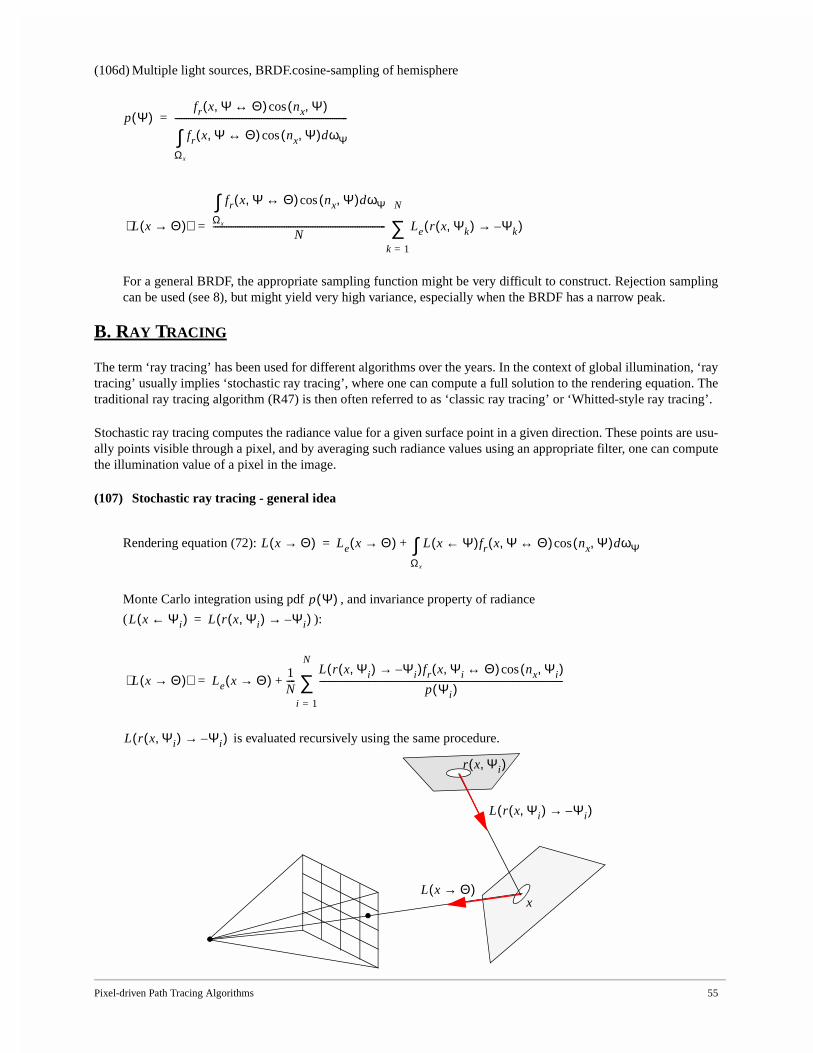
Pixel-driven Path Tracing Algorithms 55

(106d) Multiple light sources, BRDF.cosine-sampling of hemisphere

For a general BRDF, the appropriate sampling function might be very difficult to construct. Rejection samplingcan be used (see 8), but might yield very high variance, especially when the BRDF has a narrow peak.

B. RAY TRACING

The term ‘ray tracing’ has been used for different algorithms over the years. In the context of global illumination, ‘raytracing’ usually implies ‘stochastic ray tracing’, where one can compute a full solution to the rendering equation. Thetraditional ray tracing algorithm (R47) is then often referred to as ‘classic ray tracing’ or ‘Whitted-style ray tracing’.

Stochastic ray tracing computes the radiance value for a given surface point in a given direction. These points are usu-ally points visible through a pixel, and by averaging such radiance values using an appropriate filter, one can computethe illumination value of a pixel in the image.

(107) Stochastic ray tracing - general idea

Rendering equation (72):

Monte Carlo integration using pdf , and invariance property of radiance

( ):

is evaluated recursively using the same procedure.

p Ψ( )fr x Ψ Θ↔,( ) nx Ψ,( )cos

fr x Ψ Θ↔,( ) nx Ψ,( )cos dωΨΩx

∫------------------------------------------------------------------------------=

L x Θ→( )⟨ ⟩

fr x Ψ Θ↔,( ) nx Ψ,( )cos dωΨΩx

∫N

------------------------------------------------------------------------------ Le r x Ψk,( ) Ψk–→( )

k 1=

N

∑=

L x Θ→( ) Le x Θ→( ) L x Ψ←( )fr x Ψ Θ↔,( ) nx Ψ,( )dωΨcos

Ωx

∫+=

p Ψ( )L x Ψi←( ) L r x Ψi,( ) Ψ– i→( )=

L x Θ→( )⟨ ⟩ Le x Θ→( ) 1N----

L r x Ψi,( ) Ψ– i→( )fr x Ψi Θ↔,( ) nx Ψi,( )cos

p Ψi( )--------------------------------------------------------------------------------------------------------------

i 1=

N

∑+=

L r x Ψi,( ) Ψ– i→( )

xL x Θ→( )

L r x Ψi,( ) Ψ– i→( )

r x Ψi,( )

Pixel-driven Path Tracing Algorithms 56

(108) Next event estimation (split in direct and indirect term)

Rewrite rendering equation (72,74) as integral over area of all light sources and hemispherical integral of allindirect light (not directly from light sources).

and .

is evaluated using any of the techniques for direct illumination (99 - 106). is

evaluated with Monte Carlo integration:

is evaluated recursively.

Some interesting choices for : uniform sampling, cosine-sampling, brdf sampling, brdf.cosine sampling.

(108a) Uniform sampling of hemisphere

(108b) Cosine-sampling of hemisphere

(cosine sampling of hemisphere, see 35)

(108c) BRDF-sampling of hemisphere

L x Θ→( ) Le x Θ→( ) Lr x Θ→( )+=

Lr x Θ→( ) L x Ψ←( )fr x Ψ Θ↔,( ) nx Ψ,( )dωΨcos

Ωx

∫=

Le y yx→( )fr x Θ xy↔,( )G x y,( )V x y,( )dAy

AL

∫ Li x Ψ←( )fr x Ψ Θ↔,( ) nx Ψ,( )dωΨcos

Ωx

∫+=

Ldirect x Θ→( ) Lindirect x Θ→( )+=

Li x Ψ←( ) Lr r x Ψi,( ) Ψ– i→( )=

Ldirect x Θ→( ) Lindirect x Θ→( )

Lindirect x Θ→( )⟨ ⟩ 1N----

Lr r x Ψi,( ) Ψ– i→( )fr x Ψi Θ↔,( ) nx Ψi,( )cos

p Ψi( )----------------------------------------------------------------------------------------------------------------

i 1=

N

∑=

Lr r x Ψi,( ) Ψ– i→( )

p Ψ( )

p Ψ( ) 12π------=

Lindirect x Θ→( )⟨ ⟩ 2πN------ Lr r x Ψi,( ) Ψ– i→( )fr x Ψi Θ↔,( ) nx Ψi,( )cos

i 1=

N

∑=

p Ψ( ) nx Ψ,( )cos π⁄=

Lindirect x Θ→( )⟨ ⟩ πN---- Lr r x Ψi,( ) Ψi–→( )fr x Ψi Θ↔,( )

i 1=

N

∑=

p Ψ( )fr x Ψ Θ↔,( )

fr x Ψ Θ↔,( )dωΨΩx

∫--------------------------------------------------=

Pixel-driven Path Tracing Algorithms 57

For a general BRDF, the appropriate sampling function might be very difficult to construct. Rejection samplingcan be used (see 8), but might yield very high variance, especially when the BRDF has a narrow peak.

(108d) Multiple light sources, BRDF.cosine-sampling of hemisphere

For a general BRDF, the appropriate sampling function might be very difficult to construct. Rejection samplingcan be used (see 8), but might yield very high variance, especially when the BRDF has a narrow peak.

(109) End of recursion - Russian Roulette

Russian Roulette is a technique that can be used to ends recursive evaluation, but still keeps the final result unbi-ased. For any (recursive) expression to be evaluated, use the following procedure:

Pick value , and generate uniform random number :

Expected value:

Global illumination context: when recursively tracing rays, Russian Roulette can be used to stop the recursion.Any value for can be used, but a popular choice is the directional-hemispherical reflectance (64) of the sur-face point where the reflection is being considered.

Another variant of looking at RR is by rescaling the function to be integrated, such that part of the integrationdomain yields , and thereby effectively stopping any further evaluations.E.g. computation of the one-dimensional integral

Using pdf :

Lindirect x Θ→( )⟨ ⟩

fr x Ψ Θ↔,( )dωΨΩx

∫N

-------------------------------------------------- Lr r x Ψi,( ) Ψi–→( ) nx Ψi,( )cos

i 1=

N

∑=

p Ψ( )fr x Ψ Θ↔,( ) nx Ψ,( )cos

fr x Ψ Θ↔,( ) nx Ψ,( )cos dωΨΩx

∫------------------------------------------------------------------------------=

Lindirect x Θ→( )⟨ ⟩

fr x Ψ Θ↔,( ) nx Ψ,( )cos dωΨΩx

∫N

------------------------------------------------------------------------------ Lr r x Ψi,( ) Ψi–→( )

i 1=

N

∑=

A

α 0 1,[ ]∈ r 0 1,[ ]∈

if r α : A⟨ ⟩≤ Aα---=

if r α : A⟨ ⟩> 0=

E A⟨ ⟩[ ] α Aα---⋅ 1 α–( ) 0⋅+ A= =

α

0

I f x( ) xd

0

1

∫ 1α--- f

xα---

xd

0

α

∫= =

p x( )

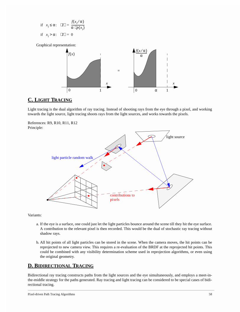
Pixel-driven Path Tracing Algorithms 58

Graphical representation:

C. LIGHT TRACING

Light tracing is the dual algorithm of ray tracing. Instead of shooting rays from the eye through a pixel, and workingtowards the light source, light tracing shoots rays from the light sources, and works towards the pixels.

References: R9, R10, R11, R12Principle:

Variants:

a. If the eye is a surface, one could just let the light particles bounce around the scene till they hit the eye surface.A contribution to the relevant pixel is then recorded. This would be the dual of stochastic ray tracing withoutshadow rays.

b. All hit points of all light particles can be stored in the scene. When the camera moves, the hit points can bereprojected to new camera view. This requires a re-evaluation of the BRDF at the reprojected hit points. Thiscould be combined with any visibility determination scheme used in reprojection algorithms, or even usingthe original geometry.

D. BIDIRECTIONAL TRACING

Bidirectional ray tracing constructs paths from the light sources and the eye simultaneously, and employs a meet-in-the-middle strategy for the paths generated. Ray tracing and light tracing can be considered to be special cases of bidi-rectional tracing.

if xi α : I⟨ ⟩≤f xi α⁄( )α p xi( )⋅--------------------=

if xi α : I⟨ ⟩> 0=

f x( )

x

f x α⁄( )α

-----------------

x

0 0 11

=

α

light particle random walk

contributions topixels

light source

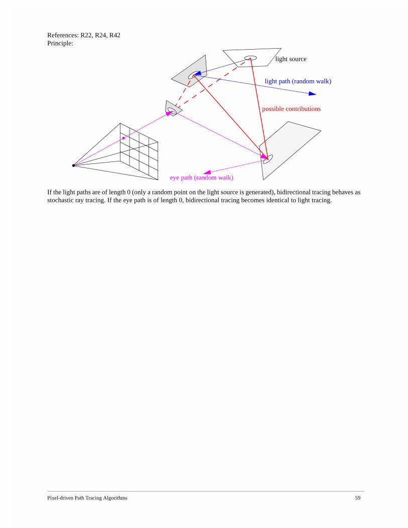
Pixel-driven Path Tracing Algorithms 59

References: R22, R24, R42Principle:

If the light paths are of length 0 (only a random point on the light source is generated), bidirectional tracing behaves asstochastic ray tracing. If the eye path is of length 0, bidirectional tracing becomes identical to light tracing.

light path (random walk)

light source

eye path (random walk)

possible contributions

Multipass Algorithms 60

XIV. Multipass Algorithms

Multipass algorithms denote a class of algorithms that combine several global illumination passes into a single solu-tion. Different passes are selected to compute subsets of all light paths. Clever combinations of different passes havebeen the subject of many global illumination papers. Often, one or more passes are used to store partial illuminationinformation in the scene, which is then read out by a subsequent pass.

To classify the different types of lightpaths, regular expressions can be used based on Heckbert’s notation (R19). Seealso (R38).

: diffuse reflection, transmission

: glossy reflection, transmission

: specular reflection, transmission

:

: the eye

: a light source

: zero or more occurences

: one or more occurences

: “or”

A. PHOTON MAPPING

Photon mapping traces light particles or photons through the scenes, and stores all possible hits of the random walks.During a subsequent stochastic ray tracing pass, information from the stored photons is used to compute several light-ing illumination components.

References: R20

D D, r Dt,

G G, r Gt,

S Sr St, ,

X D S G( )E

L

*

+

|

Test Scenes for Global Illumination 61

XV. Test Scenes for Global Illumination

(110) Mother of all test scenes

Data for the original Cornell Box can be found at:

http://www.graphics.cornell.edu/online/box/

(111) Analytic Solution - General Rendering Equation

If and if the environment is closed, then:

is the solution for (72).

For diffuse surfaces:

In other words, every surface point emits exactly the amount of energy that is absorbed at the point.

(112) Analytic Solution - Radiosity System

if and if the environment is closed, then:

is the solution for the linear system (93).

(113) Testing global illumination algorithms

Brian Smits and Henrik Jensen have proposed a number of simple and elegant scenes to test light transportmodes (R36), available at the following URL: http://www.cs.utah.edu/~bes/papers/scenes/.

A number of scenes, designed to test performance and overall image appearance, made available by Greg WardLarson and Peter Shirley are available from the RADIANCE website: http://radsite.lbl.gov/mgf/.

Andrew Willmott and Paul Heckbert have designed parametrized test scenes for diffuse global illumination(radiosity), so that algorithms' sensitivity to various parameters, such as reflectance or scene complexity, can betested. They also described a scheme for making comparisons that normalizes for differences in error and time.All information can be found at the following URL: http://www.cs.cmu.edu/~radiosity/.

(114) Testing ray tracing performance

The classic Standard Procedural Database (R17), designed by Eric Haines to test the performance of classic raytracers, is available from: http://www.acm.org/tog/resources/SPD/overview.html.

(115) Testing animated ray tracing

Jonas Lext, Ulf Assarsson, and Tomas Möller have designed a number of scenes to test animated ray tracing.http://www.ce.chalmers.se/BART/.

x Θ,( ):∀ Le x Θ→( ) dωΨfr x Ψ Θ↔,( ) nx Ψ,( )cos

Ωx

∫+ 1=

L x Θ→( ) 1≡ L x Θ→( ) Le x Θ→( ) dωΨL x Ψ←( )fr x Ψ Θ↔,( ) nx Ψ,( )cos

Ωx

∫+=

x Θ,( ):∀ Le x Θ→( ) ρd+ 1=

patches i:∀ Pei ρi+ 1=

i:∀ Pi 1= Pi Pei ρi Fj i→ Pj

j

∑+=

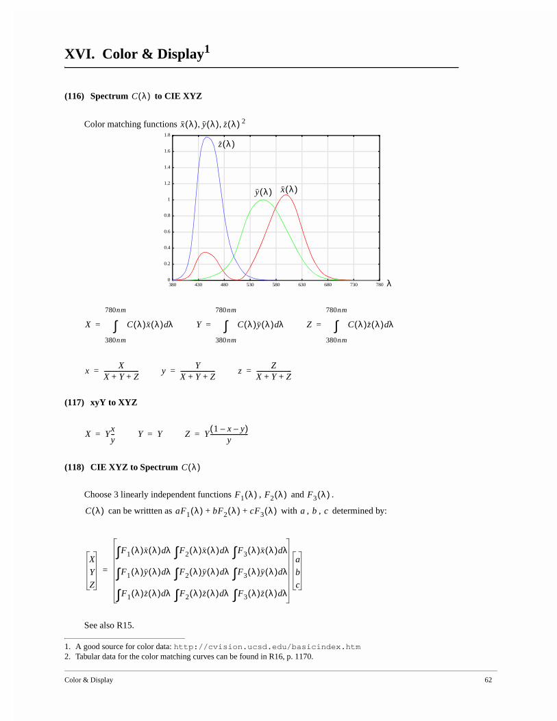
Color & Display 62

XVI. Color & Display1

(116) Spectrum to CIE XYZ

Color matching functions 2

(117) xyY to XYZ

(118) CIE XYZ to Spectrum

Choose 3 linearly independent functions , and .

can be writtten as with , , determined by:

See also R15.

1. A good source for color data: http://cvision.ucsd.edu/basicindex.htm2. Tabular data for the color matching curves can be found in R16, p. 1170.

C λ( )

x λ( ) y λ( ) z λ( ),,

0

0.2

0.4

0.6

0.8

1

1.2

1.4

1.6

1.8

380 430 480 530 580 630 680 730 780

x λ( )y λ( )

λ

z λ( )

X C λ( )x λ( ) λd

380nm

780nm

∫= Y C λ( )y λ( ) λd

380nm

780nm

∫= Z C λ( )z λ( ) λd

380nm

780nm

∫=

xX

X Y Z+ +-----------------------= y

YX Y Z+ +-----------------------= z

ZX Y Z+ +-----------------------=

X Yxy--= Y Y= Z Y

1 x– y–( )y

-------------------------=

C λ( )

F1 λ( ) F2 λ( ) F3 λ( )

C λ( ) aF1 λ( ) bF2 λ( ) cF3 λ( )+ + a b c

X

Y

Z

F1 λ( )x λ( ) λd∫ F2 λ( )x λ( ) λd∫ F3 λ( )x λ( ) λd∫F1 λ( )y λ( ) λd∫ F2 λ( )y λ( ) λd∫ F3 λ( )y λ( ) λd∫F1 λ( )z λ( ) λd∫ F2 λ( )z λ( ) λd∫ F3 λ( )z λ( ) λd∫

a

b

c

=

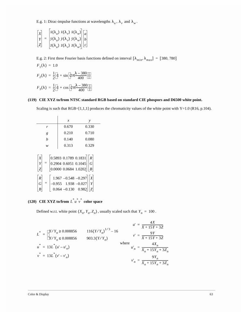
Color & Display 63

E.g. 1: Dirac-impulse functions at wavelengths , and .

E.g. 2: First three Fourier basis functions defined on interval

(119) CIE XYZ to/from NTSC standard RGB based on standard CIE phospors and D6500 white point.

Scaling is such that RGB=[1,1,1] produces the chromaticity values of the white point with Y=1.0 (R16, p.104).

(120) CIE XYZ to/from color space

Defined w.r.t. white point , usually scaled such that .

where

x y

r 0.670 0.330

g 0.210 0.710

b 0.140 0.080

w 0.313 0.329

λu λv λw

X

Y

Z

x λu( ) x λv( ) x λw( )

y λu( ) y λv( ) y λw( )

z λu( ) z λv( ) z λw( )

a

b

c

=

λmin λmax,[ ] 380 780,[ ]=

F1 λ( ) 1.0=

F2 λ( ) 12--- 1 2πλ 380–

400------------------

sin+ =

F3 λ( ) 12--- 1 2πλ 380–

400------------------

cos+ =

X

Y

Z

0.5893 0.1789 0.1831

0.2904 0.6051 0.1045

0.0000 0.0684 1.0202

R

G

B

=

R

G

B

1.967 0.548– 0.297–

0.955– 1.938 0.027–

0.064 0.130– 0.982

X

Y

Z

=

L*u

*v

*

Xn Yn Zn, ,( ) Yn 100=

L* Y Yn⁄ 0.008856≥ 116 Y Yn⁄( )1 3⁄

16–

Y Yn⁄ 0.008856≤ 903.3 Y Yn⁄( )

=

u*

13L*

u' u'n–( )=

v*

13L*

v' v'n–( )=

u' 4XX 15Y 3Z+ +--------------------------------=

v' 9YX 15Y 3Z+ +--------------------------------=

u'n4Xn

Xn 15Yn 3Zn+ +----------------------------------------=

v'n9Yn

Xn 15Yn 3Zn+ +----------------------------------------=

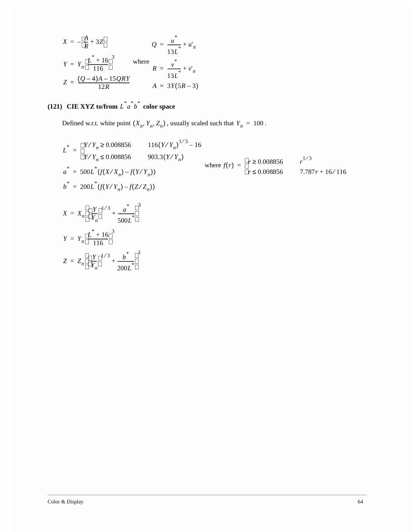
Color & Display 64

where

(121) CIE XYZ to/from color space

Defined w.r.t. white point , usually scaled such that .

where

XAR--- 3Z+

–=

Y YnL

*16+

116------------------

3

=

ZQ 4–( )A 15QRY–

12R----------------------------------------------=

Qu

*

13L*

------------ u'n+=

Rv

*

13L*

------------ v'n+=

A 3Y 5R 3–( )=

L*a

*b

*

Xn Yn Zn, ,( ) Yn 100=

L* Y Yn⁄ 0.008856≥ 116 Y Yn⁄( )1 3⁄

16–

Y Yn⁄ 0.008856≤ 903.3 Y Yn⁄( )

=

a*

500L*

f X Xn⁄( ) f Y Yn⁄( )–( )=

b*

200L*

f Y Yn⁄( ) f Z Zn⁄( )–( )=

f r( ) r 0.008856≥ r1 3⁄

r 0.008856≤ 7.787r 16 116⁄+

=

X XnYYn-----

1 3⁄ a*

500L*

---------------+ 3

=

Y YnL

*16+

116------------------

3

=

Z ZnYYn-----

1 3⁄ b*

200L*

---------------+ 3

=

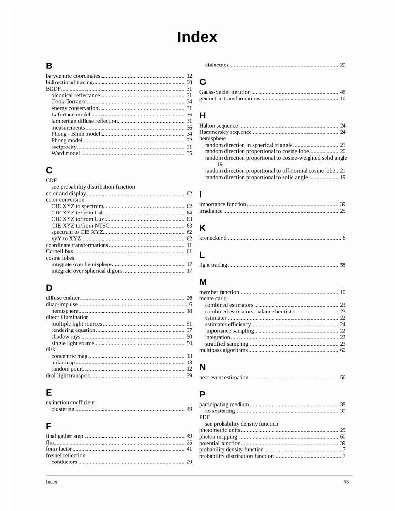
Index 65

Index

Bbarycentric coordinates.......................................................... 12bidirectional tracing............................................................... 58BRDF..................................................................................... 31

biconical reflectance.......................................................... 31Cook-Torrance................................................................... 34energy conservation........................................................... 31Lafortune model ................................................................ 36lambertian diffuse reflection.............................................. 31measurements .................................................................... 36Phong - Blinn model.......................................................... 34Phong model...................................................................... 32reciprocity.......................................................................... 31Ward model ....................................................................... 35

CCDF

see probability distribution functioncolor and display ................................................................... 62color conversion

CIE XYZ to spectrum........................................................ 62CIE XYZ to/from Lab ....................................................... 64CIE XYZ to/from Luv....................................................... 63CIE XYZ to/from NTSC ................................................... 63spectrum to CIE XYZ........................................................ 62xyY to XYZ....................................................................... 62

coordinate transformations .................................................... 11Cornell box ............................................................................ 61cosine lobes

integrate over hemisphere.................................................. 17integrate over spherical digons .......................................... 17

Ddiffuse emitter........................................................................ 26dirac-impulse ........................................................................... 6

hemisphere......................................................................... 18direct illumination

multiple light sources ........................................................ 51rendering equation............................................................. 37shadow rays ....................................................................... 50single light source.............................................................. 50

diskconcentric map .................................................................. 13polar map........................................................................... 13random point...................................................................... 12

dual light transport................................................................. 39

Eextinction coefficient

clustering ........................................................................... 49

Ffinal gather step ..................................................................... 49flux......................................................................................... 25form factor............................................................................. 41fresnel reflection

conductors ......................................................................... 29

dielectrics........................................................................... 29

GGauss-Seidel iteration............................................................ 48geometric transformations ..................................................... 10

HHalton sequence..................................................................... 24Hammersley sequence ........................................................... 24hemisphere

random direction in spherical triangle ............................... 21random direction proportional to cosine lobe.................... 20random direction proportional to cosine-weighted solid angle

19random direction proportional to off-normal cosine lobe.. 21random direction proportional to solid angle..................... 19

Iimportance function ............................................................... 39irradiance ............................................................................... 25

Kkronecker d .............................................................................. 6

Llight tracing............................................................................ 58

Mmember function.................................................................... 10monte carlo

combined estimators .......................................................... 23combined estimators, balance heuristic ............................. 23estimator ............................................................................ 22estimator efficiency............................................................ 24importance sampling.......................................................... 22integration .......................................................................... 22stratified sampling ............................................................. 23

multipass algorithms.............................................................. 60

Nnext event estimation ............................................................. 56

Pparticipating medium ............................................................. 38

no scattering....................................................................... 39PDF

see probability density functionphotometric units ................................................................... 25photon mapping ..................................................................... 60potential function ................................................................... 39probability density function..................................................... 7probability distribution function .............................................. 7

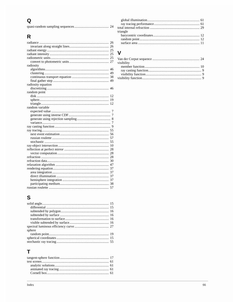
Index 66

Qquasi-random sampling sequences ........................................ 24

Rradiance ................................................................................. 26

invariant along straight lines.............................................. 26radiant energy ........................................................................ 25radiant intensity ..................................................................... 25radiometric units.................................................................... 25

convert to photometric units .............................................. 27radiosity

algorithms.......................................................................... 46clustering ........................................................................... 49continuous transport equation ........................................... 38final gather step ................................................................. 49

radiosity equationdiscretizing ........................................................................ 46

random pointdisk .................................................................................... 12sphere................................................................................. 19triangle............................................................................... 12

random variableexpected value ..................................................................... 7generate using inverse CDF................................................. 7generate using rejection sampling ....................................... 8variance................................................................................ 7

ray casting function ................................................................. 9ray tracing.............................................................................. 55

next event estimation ......................................................... 56russian roulette .................................................................. 57stochastic ........................................................................... 55

ray-object intersection ........................................................... 10reflection at perfect mirror .................................................... 28

vector computation ............................................................ 28refraction ............................................................................... 28refraction data........................................................................ 30relaxation algorithm .............................................................. 47rendering equation................................................................. 37

area integration .................................................................. 37direct illumination ............................................................. 37hemisphere integration ...................................................... 37participating medium......................................................... 38

russian roulette ...................................................................... 57

Ssolid angle.............................................................................. 15

differential ......................................................................... 15subtended by polygon........................................................ 16subtended by surface ......................................................... 16transformation to surface................................................... 16visible subtended by surface.............................................. 16

spectral luminous efficiency curve ........................................ 27sphere

random point...................................................................... 19spherical coordinates ............................................................. 15stochastic ray tracing ............................................................. 55

Ttangent-sphere function ......................................................... 17test scenes .............................................................................. 61

analytic solutions............................................................... 61animated ray tracing .......................................................... 61Cornell box ........................................................................ 61

global illumination............................................................. 61ray tracing performance..................................................... 61

total internal refraction .......................................................... 29triangle

barycentric coordinates...................................................... 12random point ...................................................................... 12surface area ........................................................................ 11

VVan der Corput sequence ....................................................... 24visibility

member function................................................................ 10ray casting function.............................................................. 9visibility function................................................................. 9

visibility function..................................................................... 9

67

References

Abbreviations:

SIGGRAPH xx: Proceedings of SIGGRAPH conference held in 19xxEGWR xx: Proceedings of the Eurographics Workshop on Rendering held in 19xxEG xx: Proceedings of the Eurographics conference held in 19xx

[1] Arvo J.; Stratified Sampling of Spherical Triangles; SIGGRAPH 95

[2] Arvo J.; Applications of Irradiance Tensors to the Simulation of Non-Lambertian Phenomena; SIGGRAPH 95

[3] Baum D., Rushmeier H., Winget J.; Improving Radiosity Solutions Through the Use of Analytically Determined Form-Fac-tors; SIGGRAPH 89

[4] Bekaert Ph., Dutré Ph., Willems Y.; Final Radiosity Gather Step using a Monte Carlo Technique with Optimal ImportanceSampling; Report CW275, January 1996, Dept. of Computer Science, Katholieke Universiteit Leuven.

[5] Bekaert Ph.; Hierarchical and Stochastic Algorithms for Radiosity; Ph.D. Thesis, Katholieke Universiteit Leuven, 1999http://www.cs.kuleuven.ac.be/cwis/research/graphics/CGRG.PUBLICATIONS/PHBPHD/

[6] Carvalho, P., Cavalcanti, P.; Point in Polyhedron Testing Using Spherical Polygons; Graphics Gems V, p. 42-49

[7] Cohen M., Wallace J.; Radiosity and Realistic Image Synthesis; Academic Press

[8] Cook R.L., Torrance K.E.; A reflectance model for computer graphics; Computer Graphics, Vol. 15, No. 3, 1981, pp. 307-316 (SIGGRAPH 81)

[9] Dutré Ph., Lafortune E., Willems Y.; Monte Carlo Light Tracing with Direct Computation of Pixel Intensities; Proceedingsof CompuGraphics, pp. 128-137, Alvor, Portugal, December 1993

[10] Dutré Ph., Willems Y.; Importance-driven Light Tracing; EGWR 94

[11] Dutré Ph., Willems Y.; Potential-driven Monte Carlo Particle Tracing for Diffuse Environments with Adaptive ProbabilityFunctions; EGWR 95

[12] Dutré Ph.; Mathematical Frameworks and Monte Carlo Algorithms for Global Illumination in Computer Graphics; Ph.D.Thesis, Katholieke Universiteit Leuven, 1996.http://www.cs.kuleuven.ac.be/~graphics/CGRG.PUBLICATIONS/PHDPHD/

[13] Dutré Ph., Bekaert Ph., Bala K.; Advanced Global Illumination; A K Peters 2003http://www.advancedglobalillumination.com/

[14] Fishman G.S.; Monte Carlo: Concepts, Algorithms and Applications; Springer-Verlag, 1996

[15] Glassner A.; How to Derive a Spectrum from an RGB Triplet; IEEE CG&A, 9(4):95-99, July 1989

[16] Glassner A.; Principles of Digital Image Synthesis; Morgan Kaufmann

[17] Haines, E. A Proposal for Standard Graphics Environments; IEEE Computer Graphics and Applications, vol. 7, no. 11,November 1987, pp. 3-5

[18] Hammersley J.M., Handscomb D.C.; Monte Carlo Methods; Chapman and Hall, London, 1964

[19] Heckbert P.; Adaptive radiosity textures for bidirectional ray tracing, SIGGRAPH 90.

[20] Jensen H.W.; Realistic Image Synthesis using Photon Mapping; AK Peters, 2001

[21] Kalos M.H., Whitlock P.A.; Monte Carlo Methods; Wiley-Interscience, New York, 1986

[22] Lafortune E.P., Willems Y.D.; Bi-directional Path Tracing; Proceedings of CompuGraphics, pp. 145-153, Alvor, Portugal,December 1993

[23] Lafortune E.P., Willems Y.D.; Using the Modified Phong Reflectance Model for Physically Based Rendering; Report CW197, November 1994, Department of Computer Science, Katholieke Universiteit Leuven.

[24] Lafortune E.; Mathematical Models and Monte Carlo Algorithms for Physically Based Rendering; Ph.D. Thesis, Katho-lieke Universiteit Leuven, 1996.

[25] Lafortune E., Foo S., Torrance K., Greenberg D.; Non-Linear Approximation of Reflectance Functions; SIGGRAPH 97

[26] Lewis R.; Making Shaders More Physically Plausible; Computer Graphics Forum, 13 (2), 1994 (also in EGWR 93)

[27] Miller, Robert D.; Computing the Area of a Spherical Polygon; Graphics Gems IV, p. 132-137

68

[28] Sbert M.; The use of global random directions to compute radiosity - Global Monte Carlo techniques. Universitat Politèc-nica de Catalunya, Barcelona, Spain, 1997.http://ima.udg.es/~mateu/

[29] Schröder P., Hanrahan P.; On the Form Factor between Two Polygons; SIGGRAPH 93

[30] Shirley P., Wang C., Zimmerman K.; Monte Carlo Techniques for Direct Lighting Calculations; ACM Transactions onGraphics, Vol. 15,1, January 1996.

[31] Shirley P.; Realistic Ray Tracing; A.K.Peters 2000

[32] Siegel R., Howell J.R.; Thermal Radiation Heat Transfer; Hemisphere Publishing Corporation

[33] Sillion F. and Puech C.; Radiosity & Global Illumination; Morgan-Kaufmann

[34] Sillion F., Drettakis G., Soler C.; A Clustering Algorithm for Radiance Calculation in General Environments; EGWR 95

[35] Sillion F.; A Unified Hierarchical Algorithm for Global Illumination with Scattering Volumes and Object Clusters; IEEETransactions on Vizualizations and Computer Graphics, 1(3), September 1995 (also in EGWR 94)

[36] Smits, B. and Jensen, H. W.; Global Illumination Test Scenes; Tech. Rep. UUCS-00-013, Computer Science Department,University of Utah, June 2000

[37] Spanier J., Gelbard E.M.; Monte Carlo Principles and Neutron Transport Problems; Addison-Wesley, 1969

[38] Suykens F., Willems Y.; Weighted Multipass Methods for Global Illumination; EG 99.

[39] Tobler R., Neumann L., Sbert M., Purgathofer W.; A New Form Factor Analogy and its Application to Stochastic GlobalIllumination Algorithms, EGWR 98

[40] Turk G.; Generating Random Points in Triangles; Graphics Gems I, p.24

[41] Ureña C., Torres J.; Improved Irradiance Computation by Importance Sampling; EGWR 97

[42] Veach E., Guibas L.; Bidirectional Estimators for Light Transport; EGWR 95

[43] Veach E., L. Guibas L.; Optimally Combining Sampling Techniques for Monte Carlo Rendering; SIGGRAPH 95

[44] Veach E.; Robust Monte Carlo Methods for Light Transport Simulation; Ph.D. Dissertation, Stanford University, December1997.

[45] Ward G.; Adaptive Shadow Testing for Ray Tracing; Photorealistic Rendering in Computer Graphics. P. Brunet and F.W.Jansen, eds. Springer-Verlag (EGWR 91)

[46] Ward G.; Measuring and Modeling Anisotropic Reflection; SIGGRAPH 92

[47] Whitted T.; An improved illumination model for shaded display; Communications of the ACM, 23(6):343-349, June 1980

[48] Zimmerman K., Shirley P.; A Two-pass Solution to the Rendering Equation with a Source Visibility Preprocess; EGWR 95