Global flow of the parabolic restricted three body problem · ow of the parabolic restricted three body problem E. Barrab es 1 J.M. Cors 2 L. Garcia1 M. Oll e2 1Universitat de Girona

Introduction Dynamics of the parabolic problem Numerical results Conclusions

Global flow of the parabolic restricted three bodyproblem

E. Barrabes 1 J.M. Cors 2 L. Garcia1 M. Olle2

1Universitat de Girona

2Universitat Politecnica de Catalunya

Ddays 2016

Barrabes, Cors, Garcia, Olle (November 10, 2016) Parabolic problem 1 / 36


Outline

Introduction

Dynamics of the parabolic problem

Numerical results

Conclusions



N-Body Problem

N-body problem: N point masses mi, i = 1, . . . N moving under theirgravitational atractions

miqi =

n∑j=1j 6=i

Gmimj(qj − qi)

r3ij

2-body problem: integrable problem. The masses move in Keplerianorbits: elliptic, parabolic or hyperbolic, around their center of mass.

Restricted Three-Body problem: Two main bodies (primaries) moving ina keplerian orbit + massless particle moving under the gravitationalattraction of the primaries, without affecting them.



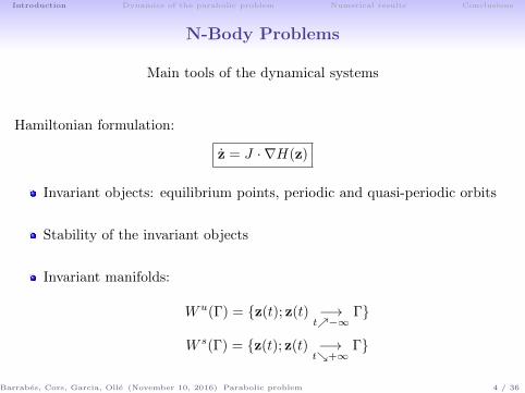
N-Body Problems

Main tools of the dynamical systems

Hamiltonian formulation:

z = J · ∇H(z)

Invariant objects: equilibrium points, periodic and quasi-periodic orbits

Stability of the invariant objects

Invariant manifolds:

Wu(Γ) = z(t); z(t) −→t−∞

Γ

W s(Γ) = z(t); z(t) −→t+∞

Γ



Galactic encounters: bridges and tails

10

NGC 2535/6 NGC 7752/3

astromania.deyave.com/ www.etsu.edu/physics/bsmith/research/sg/arp.html www.spiral-galaxies.com/Galaxies-Pegasus.html

NGC 3808

Bridges!



Galactic encounters: bridges and tails

9

Tails!

Arp 173

• NGC 2992/3

http://www.astrooptik.com/Bildergalerie/PolluxGallery/NGC2623.htm www.etsu.edu/physics/bsmith/research/sg/arp.html

http://www.ess.sunysb.edu/fwalter/SMARTS/findingcharts.html

NGC 2623



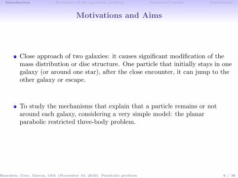
Motivations and Aims

Close approach of two galaxies: it causes significant modification of themass distribution or disc structure. One particle that initially stays in onegalaxy (or around one star), after the close encounter, it can jump to theother galaxy or escape.

To study the mechanisms that explain that a particle remains or notaround each galaxy, considering a very simple model: the planarparabolic restricted three-body problem.



Outline

Introduction


Numerical results

Conclusions



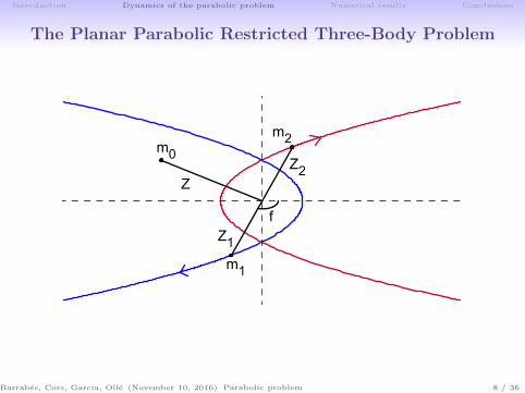
The Planar Parabolic Restricted Three-Body Problem



Equations (I)

Parabolic problem:

d2Z

dt2= −(1− µ)

Z− Z1

|Z− Z1|3− µ Z− Z2

|Z− Z2|3,

Z2 = −Z1 = 12 (σ2 − 1, 2σ), and σ = tan(f/2)

Change to a synodic frame (primaries at fixed positions) + change of time:

z1 = (−1

2, 0), z2 = (

1

2, 0),

dt

ds=√

2 r3/2.

Compatification to extend the flow when the primaries are at infinity(t, s→ ±∞):

sin(θ) = tanh(s).



Equations (II)

Global system

θ′ = cos θ,z′ = w,w′ = −A(θ)w +∇Ω(z)

where ′ =d

dsand

A(θ) =

(sin θ 4 cos θ−4 cos θ sin θ

),

Ω(z) = x2 + y2 + 21− µ√

(x− µ)2 + y2+ 2

µ√(x− µ+ 1)2 + y2

.



Upper and Lower boundary problems

Global system Boundary problems θ′ = cos θ,z′ = w,w′ = −A(θ)w +∇Ω(z)

−→θ=±π/2

z′ = w,w′ = ∓w +∇Ω(z)

dim 5 dim 4



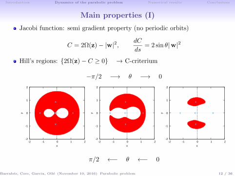
Main properties (I)

Jacobi function: semi gradient property (no periodic orbits)

C = 2Ω(z)− |w|2, dC

ds= 2 sin θ|w|2

Hill’s regions: 2Ω(z)− C ≥ 0 → C-criterium

−π/2 −→ θ −→ 0

-2

-1

0

1

2

-2 -1 0 1 2

y

x

-2

-1

0

1

2

-2 -1 0 1 2

y

x

-2

-1

0

1

2

-2 -1 0 1 2

y

x

π/2 ←− θ ←− 0



Main properties (II)

Equilibrium points at the boundaries (as in the RTBP):

Collinear: L±i = (xi(µ), 0, 0, 0,±π/2), i = 1, 2, 3

Triangular: L±i = (µ− 12 ,±√

3/2, 0, 0,±π/2), i = 4, 5

Stability:

L+1,2,3 L+

4,5

dim(Wu) 1 2dim(W s) 4 3

L−1,2,3 L−4,5dim(Wu) 4 3dim(W s) 1 2



Main properties (II)

Equilibrium points at the boundaries: L±i , i = 1, ..., 5 for θ = ±π/2 andµ = 1/2

(xi, yi) C(L±i ) = CiL±1 (−1.198406145, 0) 6.91359245

L±2 (0, 0) 8

L±3 (1.198406145, 0) 6.91359245

L±4,5 (0,±√

3/2) 5.5



Main properties (III)

Homothetic solutions and connections

θ = π/2

θ = −π/2

θ = 0

L+1

L+4

L+3

L−3L−

4

L−1



Dynamics of the problem

In order to describe the dynamics of the parabolic problem, we will focus ontwo aspects:

the final evolutions in the synodical system when time tends to infinity,

the richness in the intermediate stages due to

existence of invariant manifolds associated with the homothetic solutions

heteroclinic connections that allow the existence of orbits with passagesclose to collinear and/or equilateral configurations.



Final evolutions

Proposition (Final evolutions)

Let γ(s) = (θ(s), z(s),w(s)), s ∈ [0,∞), be a solution ofthe global system. Then, either:

it is a collision orbit,

lims→∞ |z(s)| =∞ (escape orbit)

its ω-limit is an equilibrium point.



Final evolutions

DefinitionLet Z(t) be a solution of the parabolic problem. We say that

it is a capture orbit around the primary of mass mi, fori = 1 or 2, if lim supt→∞ |Z(t)− Zi(t)| ≤ K, for someconstant K;

it is an escape orbit if lim supt→∞ |Z(t)| =∞ andlim supt→∞ |Z(t)− Zi(t)| =∞ for i = 1 and 2.

Remark: the definition is given in the inertial frame: |Z− Zi| = r|z− zi|capture orbit → |z− zi| → 0 (collision orbit)

lim infs→∞ |z(s)| ≥ K → escape orbit



C-criterium

Proposition

Let q ∈ Int(D) with θ ≥ 0, and γ(s) = (θ(s), z(s),w(s)),s ∈ [0,∞), the solution of the global system through q. Then,

(i) if for some time s0 the value of the Jacobi functionC(γ(s0)) > C2 and z(s) is located in one of the boundedcomponents of the Hill’s region, then it is a collision orbit;

(ii) if for some time s0 the value of the Jacobi functionC(γ(s0)) > C3 and z(s) is located in the unboundedcomponent of the Hill’s region, then it is an escape orbit.



Connections in the the upper boundary problem

m1 m2∞

m1 ∞ m2

L+4

L+5

L+1 L+

3

L+2



Heteroclinic L+4 → L+

3

Invariant manifold Wu(L+4 ) (dim=2) and its intersections with

ΣC∗ = (z,w) | C(z,w) = C∗

0

0.5

1

1.5

2

-1.5 -1 -0.5 0 0.5 1 1.5

y

x

C=6.0

C=6.5C=6.8




3


ΣC∗ = (z,w) | C(z,w) = C∗

-2

-1.5

-1

-0.5

0

0.5

1

1.5

2

-2 -1.5 -1 -0.5 0 0.5 1 1.5 2

y

x

C=6.9

-2

-1.5

-1

-0.5

0

0.5

1

1.5

2

-2 -1.5 -1 -0.5 0 0.5 1 1.5 2

y

x

C=6.913




3


ΣC∗ = (z,w) | C(z,w) = C∗

-0.2

-0.1

0

0.1

1.1 1.15 1.2 1.25 1.3 1.35

y

x

-0.2

-0.1

0

0.1

1.1 1.15 1.2 1.25 1.3 1.35

y

x



Outline

Introduction


Numerical results

Conclusions



Explorations

Role of the invariant manifolds in the sets of connecting orbits betweenprimaries

Equal masses (µ = 0.5):Barrabes, Cors, Olle Dynamics of the parabolic restricted three-bodyproblem Communications in Nonlinear Science and Numerical Simulation,29: 400–415, 2015

Different masses (µ < 0.5):



Connecting orbits with passages to collinear or triangularconfigurations

Connection of type mi − Lk −mj :

collision orbit with mi backwards in time

collision orbit with mj forwards in time

along its trajectory it has a close passage to Lk



Connecting orbits: examples (µ = 0.5)

-0.5

-0.25

0

0.25

0.5

-0.25 0 0.25 0.5 0.75

y

x

-4

-2

0

2

4

-10 -6 -2 2 6 10

YX

m2

m0

m1

m2

m0

m1

m0

m2

m1

m2 − L2 −m2




-1

-0.5

0

0.5

-0.5 0 0.5 1

y

x

m2 − L3 − L2 −m2/m1




-4

-2

0

2

4

-4 -2 0 2 4

m1

m0

m2

-3000

-1500

0

1500

3000

-3e+06 -1.5e+06 0 1.5e+06 3e+06

Y

X

m1

m2

m0

-30

-15

0

15

30

-200 -100 0 100 200

m1

m2

m0



Symmetric connecting orbits (µ = 0.5)

Connection mi −mi: crosses the section θ = 0 such that y = x′ = 0

I.C. (x0, 0, 0, y′0)

Connection mi −mj : crosses the section θ = 0 such that x = y′ = 0

I.C. (0, y0, x′0, 0)




mi −mi

-6

-4

-2

0

2

4

6

-4 -3 -2 -1 0 1 2 3 4

y’

x

-0.4

-0.3

-0.2

-0.1

0

0.1

0.2

0.3

0.4

0.3 0.4 0.5 0.6 0.7 0.8 0.9 1 1.1

-4

-3

-2

-1

0

1

2

3

4

-8 -6 -4 -2 0 2 4 6 8




mi −mj

-10

-8

-6

-4

-2

0

2

0 1 2 3 4 5

x’

y

capture m2capture m1C=C(L3)

-0.3

-0.25

-0.2

-0.15

-0.1

-0.05

0

0.05

0.1

0.15

0.2

-0.8 -0.6 -0.4 -0.2 0 0.2 0.4 0.6 0.8

-4

-3

-2

-1

0

1

2

3

4

-8 -6 -4 -2 0 2 4 6 8




-3.33108

-3.33103

-3.33098

-3.33093

0.52952 0.5296 0.52968

x’

y

a

c-b

d-e

f

-2

-1

0

1

-2 -1 0 1 2

y

x

ab

cd e f




L−3 → L+

3

L−1 → L+

1

L−2 → L+

2

L−3 → L+

1

L−1 → L+

3

L−2 → L+

2



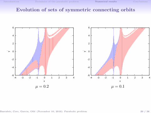
Evolution of sets of symmetric connecting orbits

-6

-4

-2

0

2

4

6

-4 -3 -2 -1 0 1 2 3 4

y’

x

-6

-4

-2

0

2

4

6

-4 -3 -2 -1 0 1 2 3 4

y’x

µ = 0.5 µ = 0.4




-6

-4

-2

0

2

4

6

-4 -3 -2 -1 0 1 2 3 4

y’

x

-6

-4

-2

0

2

4

6

-4 -3 -2 -1 0 1 2 3 4

y’x

µ = 0.3 µ = 0.2




-6

-4

-2

0

2

4

6

-4 -3 -2 -1 0 1 2 3 4

y’

x

-6

-4

-2

0

2

4

6

-4 -3 -2 -1 0 1 2 3 4

y’x

µ = 0.2 µ = 0.1



Bridges and Tails?

We consider a bunch of initial conditions around m1 for θ = −π/4 and a valueC ≥ C2 = 8 (for µ = 1/2). For this value of C, we fix a radius, r (distance tom1) and move α ∈ [0, 2π]. Since, velocity module is given by position andJacobi function C, we move β ∈ [0, 2π] (velocity direction).

0

1

2

3

4

5

6

0 1 2 3 4 5 6

β

α

0

1

2

3

4

5

6

0 1 2 3 4 5 6

β

α

r = 0.2 r = 0.001



Tails

0

1

2

3

4

5

6

0 1 2 3 4 5 6

β

α

-4

0

4

8

12

-4 0 4 8

m1

m2

yx

r = 0.2 θ = 1.2



Bridges

0

1

2

3

4

5

6

0 1 2 3 4 5 6

β

α

-4

-2

0

2

4

-4 -2 0 2 4

m1

m2

yx

r = 0.2 θ = 1.2



A Movie

-2

-1

0

1

2

-2 -1 0 1 2

y

x

m1

m2

-2

-1

0

1

2

-2 -1 0 1 2

yx

m1 m2

θ = −π/8 θ = 0



A Movie

-2

-1

0

1

2

-2 -1 0 1 2

y

x

m1

m2

-8

-6

-4

-2

0

2

4

6

8

-8 -6 -4 -2 0 2 4 6 8

yx

m1

m2

θ = π/8 θ = π/8



A Movie

-8

-4

0

4

8

-8 -4 0 4 8

y

x

m1

m2

-8

-4

0

4

8

-8 -4 0 4 8

yx

m1

m2

θ = 1.2 θ = 1.2



Outline

Introduction


Numerical results

Conclusions



Conclusions

Using the invariant manifolds, the symmetries of the problem and theC-criterium it is possible to construct connecting orbits of different types.

The regions of the phase space where the test particles remain or notaround each galaxy are confined by the invariant manifolds of thecollinear equilibrium points.



Further work

How does the mass parameter of the parabolic problem affects Bridgesand tails?

Explorations varying the inclination (Spatial parabolic problem)

Hyperbolic problem (make sense)


Documents

Global flow of the parabolic restricted three body problem · ow of the parabolic restricted three body problem E. Barrab es 1 J.M. Cors 2 L. Garcia1 M. Oll e2 1Universitat de Girona