Embed Size (px)
Citation preview
Math. Z. (2007) 256:521–549DOI 10.1007/s00209-006-0083-2 Mathematische Zeitschrift
Global existence of null-form wave equationsin exterior domains
Jason Metcalfe · Christopher D. Sogge
Received: 7 October 2005 / Accepted: 31 August 2006 /Published online: 6 January 2007© Springer-Verlag 2006
Abstract We provide a proof of global existence of solutions to quasilinear waveequations satisfying the null condition in certain exterior domains. In particular, ourproof does not require estimation of the fundamental solution for the free wave equa-tion. We instead rely upon a class of Keel–Smith–Sogge estimates for the perturbedwave equation. Using this, a notable simplification is made as compared to previ-ous works concerning wave equations in exterior domains: one no longer needs todistinguish the scaling vector field from the other admissible vector fields.
1 Introduction
Inspired by the approach of Sideris and Tu [26] in the boundaryless case and theapplication of such techniques in Sideris [25], we prove global existence for multi-speed systems of quasilinear wave equations satisfying the null condition in certainexterior domains without using estimation of the fundamental solution for the freewave equation. To do so, we use a Keel–Smith–Sogge estimate for the perturbedequation established previously by the authors in [23]. In the previous works on non-linear wave equations in exterior domains, [12], [21,22], and [19,20], it was necessaryto use estimates that involved relatively few occurrences of the scaling vector fieldL = t∂t + r∂r. A notable innovation in the new approach allows us to no longerdistinguish between the scaling vector field L and the other “admissible” invariantvector fields Z = {�ij = xi∂j − xj∂i, ∂k : 1 ≤ i, j ≤ 3, 0 ≤ k ≤ 3}. This is accomplished
J. Metcalfe (B)Department of Mathematics, University of California,Berkeley, CA 94720-3840, USAe-mail: [email protected]
C. D. SoggeDepartment of Mathematics, Johns Hopkins University,Baltimore, MD 21218, USAe-mail: [email protected]
522 J. Metcalfe, C. D. Sogge
by introducing modified vector fields that preserve the boundary condition, as was inpart done in [21].
The main existence result is an analog of the classic results of Christodoulou [3]and Klainerman [14] in the boundaryless case. In the multiple speed boundarylesscase, related results were established, e.g., by Sideris and Tu [26], Sogge [28], Agemiand Yokoyama [1], Kubota and Yokoyama [16], Hidano [4], Yokoyama [31], andKatayama [7–9]. In exterior domains, null form quasilinear wave equations were pre-viously studied by Keel et al. [10], the authors [21], and Metcalfe et al. [19,20]. Wenote that the main theorem of this paper was previously established (in a more generalcontext) in [19]. We, however, believe that the new techniques are of independentinterest, and we are hopeful about their potential use in applications.
Our proof uses Klainerman’s method of commuting vector fields [14] as wasadapted to exterior domains by Keel et al. [12]. In particular, we restrict to the classof “admissible” vector fields that was mentioned above. Notably absent in this set arethe hyperbolic rotations �0j = t∂j + xj∂t which do not seem appropriate for problemsin exterior domains as they have unbounded normal component on the boundary.Moreover, in the multiple speed setting, these vector fields have an associated speedand only commute with the d’Alembertian of the same speed.
This approach relies upon a weighted space-time L2 estimate, which will be referredto as the Keel–Smith–Sogge estimate or KSS estimate. Such estimates were estab-lished in [11] where they were first used to show long-time existence of solutions tononlinear equations. With this estimate, existence is established using O(1/|x|) decayrather than the more standard, but quite difficult to prove when there is boundary,O(1/t) decay. An earlier, related estimate is due to Strauss [30] (Lemma 3). The proofin [11] is easily modified to establish these bounds in all dimensions n ≥ 3 as is done inMetcalfe [18] and Hidano and Yokoyama [5] and has been used in, e.g., [5], [18], and[22] to study nonlinear equations. Recently, using techniques of Rodnianski [29], theauthors [23] have established an analogous estimate for the perturbed equation. Thisinequality is essential to the approach presented in this article. It is worth noting thatAlinhac [2] simultaneously obtained a related KSS-type estimate for the perturbedequation and for wave equations on curved backgrounds. The assumptions made onthe perturbation in [2] are, however, not as favorable in the current setting.
The KSS estimate and energy estimates will be coupled with some well-knowndecay estimates in order to get global existence. These decay estimates are variants ofthose of Klainerman and Sideris [15] and are known to be rather widely applicable,including e.g. to the equations of elasticity. This will, of course, be used in combinationwith the extra decay afforded to us by the null condition.
The major innovations of this paper regard the variable-coefficient KSS estimate.First, we expand upon the proof in [23] and carefully prove the KSS estimates for theperturbed wave equation in the multiple speed setting. Having such estimates for theperturbed equation allows us to apply the KSS estimates even for terms of the highestorder. This was not previously possible for quasilinear equations as there was a loss ofregularity resulting from the occurrence of second derivatives. As such, we may nowprove global existence using only energy methods. In particular, the decay estimatesthat we shall employ do not require direct estimation of the fundamental solution ofthe linear wave equation, and in particular, such estimates are known to hold for somerelated applications. We note, e.g., that the only obstacle to using similar techniques tostudy the equations of isotropic elasticity in exterior domains is deriving the existenceof a KSS-type estimate for the perturbed linearized equations. This, however, is more
Global existence of null-form wave equations in exterior domains 523
delicate than in the current setting due to the off-diagonal terms and is currently anopen problem of interest.
A key obstacle to using only energy methods in previous studies was the boundaryterms that arise in the Klainerman-Sideris estimates. In particular, there is a termlocalized near the boundary which has significantly less decay in t. To alleviate this,we shall use the additional decay in x, which was largely ignored in previous works,from the Klainerman–Sideris estimates. When combined with the KSS estimates, thisdecay permits us the necessary control over the boundary term.
As the coefficients of the scaling vector field can be large in an arbitrarily smallneighborhood of the obstacle, previous works in exterior domains using the adaptedmethod of commuting vector fields use estimates that required relatively few occur-rences of L, and during the proofs of long-time existences, the scaling vector fieldsmust be carefully tracked. This, at best, complicated these arguments. Using the vari-able coefficient KSS estimates, we show that it is not strictly necessary to differentiateL from the other admissible vector fields. In particular, we use a modified scalingvector field which preserves the Dirichlet boundary conditions as in [21], but insteadof proving boundary term estimates, such as [21, Lemma 2.9], we are now able tocontrol the resulting commutators using the variable coefficient KSS estimates.
Finally, we mention that our proof, unlike many of the previous works in exte-rior domains, does not directly use the decay of local energy, such as that of Lax,Morawetz, and Phillips [17]. Our hypotheses on the obstacle are, however, sufficientto guarantee said decay. It is conceivable that the techniques contained herein couldbe important in other applications where the rate of decay of local energy is slower,say e.g. in even dimensions.
We now more precisely describe the main result of this article. We begin by fixinga bounded obstacle K ⊂ R
3 with smooth boundary. Moreover, we shall assume thatK is star-shaped with respect to the origin. As we shall see, scaling will allow us toassume without loss that K ⊂ {|x| ≤ 1}, and this assumption is made throughout. Thestar-shapedness assumption is used to see that certain boundary terms in our energyestimates and KSS estimates have a favorable sign. This is reminiscent of argumentsfrom Morawetz [24].
In the exterior of K, we shall study systems of quasilinear wave equations of theform
⎧⎪⎨
⎪⎩
∂2t uI − c2
I�uI = BIJ,αβK,γ ∂γ uK∂α∂βuJ , (t, x) ∈ R+ × R
3\K, I = 1, 2, . . . , D,
u(t, · )|∂K = 0,u(0, · ) = f , ∂tu(0, · ) = g.
(1.1)
Here and throughout we use the Einstein summation convention. Repeated Greekindices α,β, γ , and δ are implicitly summed from 0 to 3. Repeated lowercase Latinindices a, b are summed from 1 to 3, and repeated uppercase Latin indices I, J, K aresummed from 1 to D. In the sequel, we will use � = (�c1 , . . . , �cD) to denote thevector-valued d’Alembertian, where �cI = ∂2
t − c2I�. For simplicity, we shall study
the nonrelativistic case where
c1 > · · · > cD > 0.
Straightforward modifications will allow for repeated wave speeds.
524 J. Metcalfe, C. D. Sogge
The BIJ,αβK,γ in (1.1) are real constants satisfying the symmetry conditions
BIJ,αβK,γ = BJI,αβ
K,γ = BIJ,βαKγ . (1.2)
In order to get global existence, we shall also need to assume that (1.1) satisfies thenull condition. In the nonrelativistic case, this says that the self-interactions amongthe quasilinear terms satisfy the standard null condition. That is,
BJJ,αβJ,γ ξαξβξγ = 0, whenever
ξ20
c2J
− ξ21 − ξ2
2 − ξ23 = 0, J = 1, . . . , D. (1.3)
To solve (1.1), the data must be assumed to satisfy the relevant compatibilityconditions. Letting Jku = {∂αx u : 0 ≤ |α| ≤ k}, we know that for a fixed m andformal Hm solution u of (1.1), we can write ∂k
t u(0, · ) = ψk(Jkf , Jk−1g), 0 ≤ k ≤ m,for compatibility functions ψk depending on the nonlinearity, Jkf , and Jk−1g. For(f , g) ∈ Hm × Hm−1, the compatibility condition simply requires that the ψk vanishon ∂K for 0 ≤ k ≤ m − 1. For smooth (f , g), we say that the compatibility conditionis satisfied to infinite order if this vanishing condition holds for all m. We refer thereader to [10] for a more thorough exposition on these compatibility conditions.
We are now prepared to state our main theorem.
Theorem 1.1 Let K be a fixed compact obstacle with smooth boundary that is star-shaped with respect to the origin. Assume that the BIJ,αβ
K,γ are as above. Then, there is a
constant ε0 > 0 and an integer constant N > 0 so that if the data (f , g) ∈ C∞(R3\K)satisfy the compatibility condition to infinite order and the smallness condition
∑
|α|≤N
‖〈x〉|α|∂αx ∂xf‖2 +∑
|α|≤N
‖〈x〉|α|∂αx g‖2 ≤ ε0, (1.4)
then (1.1) has a unique global solution u ∈ C∞([0, ∞)× R3\K).
This paper is organized as follows. In the next section, we provide derivations of theenergy estimates and KSS estimates for the perturbed wave equations. We also showthat an appropriate variant of these holds when u is replaced by �µu. Here � = {L, Z}is the set of admissible vector fields. As mentioned previously, the fact that we nolonger need to distinguish between L and Z is a significant innovation in this paper.In the third section, we present the decay estimates that we will require. These arefairly well-known, but in the interest of making this paper somewhat self-contained,the proofs are sketched. In the last section, we prove the main result, Theorem 1.1.
2 Energy estimates and Keel–Smith–Sogge estimates
In this section, we establish the energy and KSS estimates for the perturbed waveequation that we shall require in the sequel. We must take care to insure that ourestimates will not destroy the null structure.
We will be concerned with solutions uI ∈ C∞(R+ × R3\K) of the Dirichlet-wave
equation{(�hu)I = FI ,u|∂K = 0
(2.1)
Global existence of null-form wave equations in exterior domains 525
where
(�hu)I = (∂2t − c2
I�)uI +
D∑
J=1
3∑
α,β=0
hIJ,αβ(t, x)∂α∂βuJ . (2.2)
We shall assume that the hIJ,αβ satisfy the symmetry conditions
hIJ,αβ = hJI,αβ = hIJ,βα , (2.3)
as well as the size condition
|h| =D∑
I,J=1
3∑
α,β=0
|hαβ(t, x)| ≤ δ 1. (2.4)
We denote u = (u1, . . . , uD). Here, we are working in the Euclidean metric, andindices are raised with this metric.
We will need to define the full energy-momentum tensor associated to (2.1). Tobegin, let
Q0β [u] = ∂0uI∂βuI − 12δ0β
[|∂0u|2 − c2
I |∇xuI |2]
+ δ0γ hIJ,γ δ∂δuJ∂βuI − 12δ0βhIJ,γ δ∂γ uJ∂δuI , (2.5)
and
Qαβ [u] = −c2I∂αuI∂βuI − 1
2δαβ
[|∂0u|2 − c2
I |∇xuI |2]
+ δαγ hIJ,γ δ∂δuJ∂βuI − 12δαβhIJ,γ δ∂γ uJ∂δuI , α = 1, 2, 3. (2.6)
An elementary calculation yields
DαQαβ [u] = ∂βuI(�hu)I + (∂γ hIJ,γ δ)∂δuJ∂βuI − 12(∂βhIJ,γ δ)∂γ uJ∂δuI . (2.7)
2.1 Energy estimate
From (2.7), we are quickly able to obtain the well-known energy estimate for theperturbed wave equation.
Proposition 2.1 Assume that K is a bounded obstacle with C1-boundary. Assume alsothat the perturbation terms are as above. Suppose that u ∈ C∞ solves (2.1) and forevery t, u(t, x) = 0 for large x. Then,
‖u′(t, · )‖22 � ‖u′(0, · )‖2
2 +t∫
0
∫
R3\K|(�hu)I∂0uI | dx ds
+t∫
0
∫
R3\K
[|(∂γ hIJ,γ δ)∂δuJ∂0uI | + |(∂0hIJ,γ δ)∂γ uJ∂δuI |
]dx ds. (2.8)
Here u′ = (∂tu, ∇xu) is used to denote the full space-time gradient.
526 J. Metcalfe, C. D. Sogge
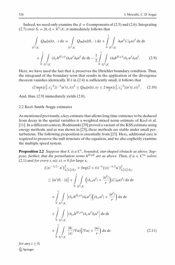
Indeed, we need only examine the β = 0 components of (2.5) and (2.6). Integrating(2.7) over St = [0, t] × R
3\K, it immediately follows that
∫
R3\KQ00[u](t, · ) dx =
∫
R3\KQ00[u](0, · ) dx +
t∫
0
∫
R3\K∂0uI(�hu)I dx ds
+t∫
0
∫
R3\K(∂γ hIJ,γ δ)∂δuJ∂0uI dx ds − 1
2
t∫
0
∫
R3\K(∂0hIJ,γ δ)∂γ uJ∂δuI . (2.9)
Here, we have used the fact that ∂t preserves the Dirichlet boundary condition. Thus,the integrand of the boundary term that results in the application of the divergencetheorem vanishes identically. If δ in (2.4) is sufficiently small, it follows that
(2 maxI
{c2I , c−2
I })−1|u′(t, x)|2 ≤ Q00[u](t, x) ≤ 2 maxI
{c2I , c−2
I }|u′(t, x)|2. (2.10)
And, thus, (2.9) immediately yields (2.8).
2.2 Keel–Smith–Sogge estimates
As mentioned previously, a key estimate that allows long time existence to be deducedfrom decay in the spatial variables is a weighted mixed norm estimate of Keel et al.[11]. In a different context, Rodnianski [29] proved a variant of the KSS estimate usingenergy methods, and as was shown in [23], these methods are stable under small per-turbations. The following proposition is essentially from [23]. Here, additional care isrequired to preserve the null structure of the equation, and we also explicitly examinethe multiple speed system.
Proposition 2.2 Suppose that K is a C1, bounded, star-shaped obstacle as above. Sup-pose, further, that the perturbation terms hIJ,αβ are as above. Then, if u ∈ C∞ solves(2.1) and for every t, u(t, x) = 0 for large x,
‖〈x〉−1/2−u′‖2L2
t L2x(St)
+ (log(2 + t))−1‖〈x〉−1/2u′‖2L2
t L2x(St)
� ‖u′(0, · )‖22 +
t∫
0
∫
R3\K
(|∂t,xuI | + |uI |
r
)|(�hu)I | dx ds
+t∫
0
∫
R3\K
∣∣∣(∂γ hIJ,γ δ)∂δuJ
∣∣∣
(|∂t,ruI | + |uI |
r
)dx ds
+t∫
0
∫
R3\K
∣∣∣(∂t,rhIJ,γ δ)∂γ uJ∂δuI
∣∣∣ dx ds
+t∫
0
∫
R3\K
|h|〈x〉 |∇u|
(|∇u| + |u|
r
)dx ds (2.11)
for any t ≥ 0.
Global existence of null-form wave equations in exterior domains 527
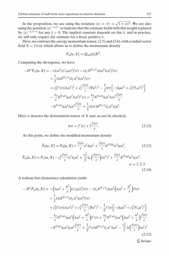
In the proposition, we are using the notation 〈x〉 = 〈r〉 = √1 + |x|2. We are also
using the notation 〈x〉−1/2− to indicate that the estimate holds with this weight replacedby 〈x〉−1/2−δ for any δ > 0. The implicit constant depends on this δ, and in practice,we will only require the estimate for a fixed, positive δ.
Here, we contract the energy momentum tensor, (2.5) and (2.6), with a radial vectorfield X = f (r)∂r which allows us to define the momentum density
Pα[u, X] = Qαβ [u]Xβ .
Computing the divergence, we have
−DαPα[u, X] = −(∂ruI)(�hu)If (r)− (∂γ hIJ,γ δ)∂δuJ∂ruIf (r)
+ 12(∂rhIJ,γ δ)∂γ uJ∂δuIf (r)
+ c2I f ′(r)(∂ruI)2 + c2
If (r)
r|�∇uI |2 − 1
2trπ
[−|∂0u|2 + c2
I |∇xuI |2]
− xa
rhIJ,aδ∂δuJ∂ruIf ′(r)+ xa
rhIJ,aδ∂δuJ∂ruI f (r)
r
− hIJ,aδ∂auI∂δuJ f (r)r
+ 12(trπ)hIJ,γ δ∂γ uJ∂δuI .
Here π denotes the deformation tensor of X and, as can be checked,
trπ = f ′(r)+ 2f (r)
r. (2.12)
At this point, we define the modified momentum density
P̃0[u, X] = P0[u, X] + f (r)r
uI∂0uI + f (r)r
hIJ,0βuI∂βuJ , (2.13)
P̃α[u, X] = Pα[u, X] − c2I
f (r)r
uI∂αuI + c2I
2∂α
( f (r)r
)(uI)2 + f (r)
rhIJ,αβuI∂βuJ ,
α = 1, 2, 3
(2.14)
A tedious but elementary calculation yields
− DαP̃α[u, X] = −(∂ruI + uI
r
)(�hu)If (r)− (∂γ hIJ,γ δ)∂δuJ
(∂ruI + uI
r
)f (r)
+ 12(∂rhIJ,γ δ)∂γ uJ∂δuIf (r)
+ c2I f ′(r)(∂ruI)2 + c2
If (r)
r|�∇uI |2 − 1
2f ′(r)
[−|∂0u|2 + c2
I |∇xuI |2]
− xa
rhIJ,aδ∂δuJ
(∂ruI + uI
r
)f ′(r)+ xa
rhIJ,aδ∂δuJ
(∂ruI + uI
r
) f (r)r
− hIJ,aδ∂auI∂δuJ f (r)r
+ 12
f ′(r)hIJ,γ δ∂γ uJ∂δuI − c2I
2�
( f (r)r
)(uI)2
(2.15)
528 J. Metcalfe, C. D. Sogge
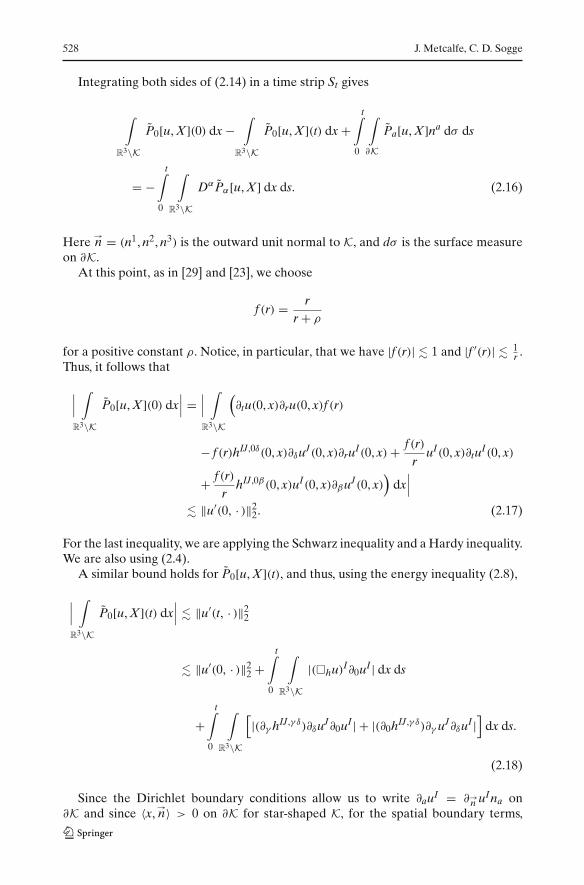
Integrating both sides of (2.14) in a time strip St gives
∫
R3\KP̃0[u, X](0) dx −
∫
R3\KP̃0[u, X](t) dx +
t∫
0
∫
∂KP̃a[u, X]na dσ ds
= −t∫
0
∫
R3\KDαP̃α[u, X] dx ds. (2.16)
Here→n = (n1, n2, n3) is the outward unit normal to K, and dσ is the surface measure
on ∂K.At this point, as in [29] and [23], we choose
f (r) = rr + ρ
for a positive constant ρ. Notice, in particular, that we have |f (r)| � 1 and |f ′(r)| � 1r .
Thus, it follows that
∣∣∣
∫
R3\KP̃0[u, X](0) dx
∣∣∣ =
∣∣∣
∫
R3\K
(∂tu(0, x)∂ru(0, x)f (r)
− f (r)hIJ,0δ(0, x)∂δuJ(0, x)∂ruI(0, x)+ f (r)r
uI(0, x)∂tuI(0, x)
+ f (r)r
hIJ,0β(0, x)uI(0, x)∂βuJ(0, x))
dx∣∣∣
� ‖u′(0, · )‖22. (2.17)
For the last inequality, we are applying the Schwarz inequality and a Hardy inequality.We are also using (2.4).
A similar bound holds for P̃0[u, X](t), and thus, using the energy inequality (2.8),
∣∣∣
∫
R3\KP̃0[u, X](t) dx
∣∣∣ � ‖u′(t, · )‖2
2
� ‖u′(0, · )‖22 +
t∫
0
∫
R3\K|(�hu)I∂0uI | dx ds
+t∫
0
∫
R3\K
[|(∂γ hIJ,γ δ)∂δuJ∂0uI | + |(∂0hIJ,γ δ)∂γ uJ∂δuI |
]dx ds.
(2.18)
Since the Dirichlet boundary conditions allow us to write ∂auI = ∂→n uIna on
∂K and since 〈x,→n〉 > 0 on ∂K for star-shaped K, for the spatial boundary terms,
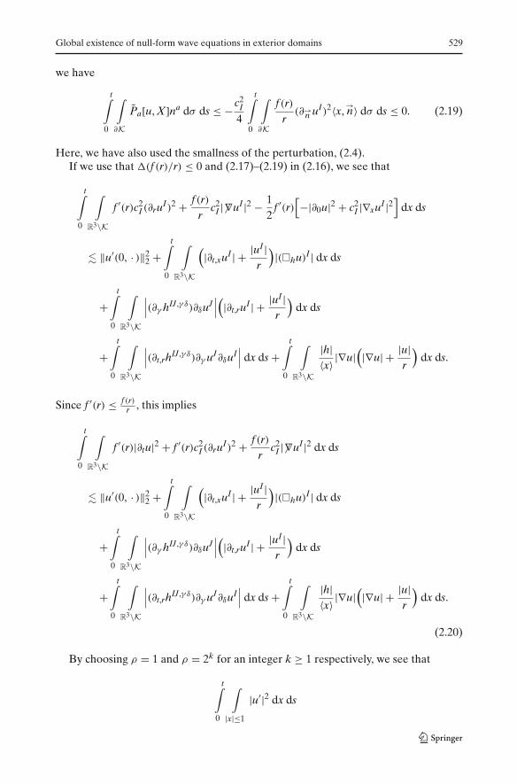
Global existence of null-form wave equations in exterior domains 529
we have
t∫
0
∫
∂KP̃a[u, X]na dσ ds ≤ −c2
I
4
t∫
0
∫
∂K
f (r)r(∂→
n uI)2〈x,→n〉 dσ ds ≤ 0. (2.19)
Here, we have also used the smallness of the perturbation, (2.4).If we use that �(f (r)/r) ≤ 0 and (2.17)–(2.19) in (2.16), we see that
t∫
0
∫
R3\Kf ′(r)c2
I (∂ruI)2 + f (r)r
c2I |�∇uI |2 − 1
2f ′(r)
[−|∂0u|2 + c2
I |∇xuI |2]
dx ds
� ‖u′(0, · )‖22 +
t∫
0
∫
R3\K
(|∂t,xuI | + |uI |
r
)|(�hu)I | dx ds
+t∫
0
∫
R3\K
∣∣∣(∂γ hIJ,γ δ)∂δuJ
∣∣∣
(|∂t,ruI | + |uI |
r
)dx ds
+t∫
0
∫
R3\K
∣∣∣(∂t,rhIJ,γ δ)∂γ uJ∂δuI
∣∣∣ dx ds +
t∫
0
∫
R3\K
|h|〈x〉 |∇u|
(|∇u| + |u|
r
)dx ds.
Since f ′(r) ≤ f (r)r , this implies
t∫
0
∫
R3\Kf ′(r)|∂tu|2 + f ′(r)c2
I (∂ruI)2 + f (r)r
c2I |�∇uI |2 dx ds
� ‖u′(0, · )‖22 +
t∫
0
∫
R3\K
(|∂t,xuI | + |uI |
r
)|(�hu)I | dx ds
+t∫
0
∫
R3\K
∣∣∣(∂γ hIJ,γ δ)∂δuJ
∣∣∣
(|∂t,ruI | + |uI |
r
)dx ds
+t∫
0
∫
R3\K
∣∣∣(∂t,rhIJ,γ δ)∂γ uJ∂δuI
∣∣∣ dx ds +
t∫
0
∫
R3\K
|h|〈x〉 |∇u|
(|∇u| + |u|
r
)dx ds.
(2.20)
By choosing ρ = 1 and ρ = 2k for an integer k ≥ 1 respectively, we see that
t∫
0
∫
|x|≤1
|u′|2 dx ds
530 J. Metcalfe, C. D. Sogge
and
t∫
0
∫
2k−1≤|x|≤2k
|u′|2r
dx ds
are bounded by the right side of (2.20). If we sum these resulting estimates over k ≥ 1,we see immediately that the bound for the first term in (2.11) holds. The same argu-ment yields the bound for the second term in the left of (2.11). Indeed, the estimatefollows trivially from (2.8) when the spatial norm is over |x| ≥ t. Thus, we need onlysum over the O(log(2 + t)) choices of k with 2k−1 � t.
2.3 Main L2 estimate
In this section, we show that higher order energy estimates also hold. In particular,we show that versions of (2.8) and (2.11) hold when u is replaced by �µu. In order todo so, we introduce modified vector fields that preserve the boundary condition. Thisextends an idea initiated in [21].
Notice that, by combining the main results [(2.8) and (2.11)] of the precedingsections, we have
‖〈x〉−1/2−u′‖2L2
t L2x(St)
+ (log(2 + t))−1‖〈x〉−1/2u′‖2L2
t L2x(St)
+ ‖u′(t, · )‖22
� ‖u′(0, · )‖22 +
t∫
0
∫
R3\K
(|∂t,xuI | + |uI |
r
)|FI | dx ds
+t∫
0
∫
R3\K
∣∣∣(∂γ hIJ,γ δ)∂δuJ
∣∣∣
(|∂t,ruI | + |uI |
r
)dx ds
+t∫
0
∫
R3\K
∣∣∣(∂t,rhIJ,γ δ)∂γ uJ∂δuI
∣∣∣ dx ds +
t∫
0
∫
R3\K
|h|〈x〉 |∇u|
(|∇u| + |u|
r
)dx ds
(2.21)
when u solves (2.1). Notice, in particular, that if F vanishes for |x| > 2, then we canbound the second term in the right side by
‖u′‖L2t L2
x(St∩{|x|≤2})‖F‖L2t L2
x(St)≤ ε‖〈x〉−1/2−u′‖2
L2t L2
x(St)+ C‖F‖2
L2t L2
x(St),
and, in this case, the first term on the right of this inequality can be bootstrapped.Here, we have used the fact that the Dirichlet boundary condition allows us tocontrol u locally by u′. We have also used that 0 ∈ K, and hence, 1/r is boundedon R
3\K.Thus, it immediately follows that if u is a solution to
{�hu = F + G
u|∂K = 0,(2.22)
Global existence of null-form wave equations in exterior domains 531
and G vanishes unless |x| ≤ 2, then
‖〈x〉−1/2−u′‖2L2
t L2x(St)
+ (log(2 + t))−1‖〈x〉−1/2u′‖2L2
t L2x(St)
+ ‖u′(t, · )‖22
� ‖u′(0, · )‖22 +
t∫
0
∫
R3\K
(|∂t,xuI | + |uI |
r
)|FI | dx ds + ‖G‖2
L2t L2
x(St)
+t∫
0
∫
R3\K
∣∣∣(∂γ hIJ,γ δ)∂δuJ
∣∣∣
(|∂t,ruI | + |uI |
r
)dx ds
+t∫
0
∫
R3\K
∣∣∣(∂t,rhIJ,γ δ)∂γ uJ∂δuI
∣∣∣ dx ds +
t∫
0
∫
R3\K
|h|〈x〉 |∇u|
(|∇u| + |u|
r
)dx ds.
(2.23)
We will use this as a base case for an induction argument to construct higher orderenergy estimates.
Since ∂ jt preserves the Dirichlet boundary condition, the estimate (2.23) holds with
u replaced by ∂ jt u. Moreover, if we apply elliptic regularity (see, e.g., [21] Lemma 2.3),
it follows that∑
|µ|≤N
‖∂µu′‖2L2
t L2x(St∩{|x|≤2}) �
∑
j≤N
‖∂ jt u
′(0, · )‖22
+∑
j,k≤N
t∫
0
∫
R3\K
(|∂k
t ∂t,xuI | + |∂kt uI |r
)|∂ j
t FI | dx ds +
∑
j≤N
‖∂ jt G‖2
L2t L2
x(St)
∑
j,k≤N
∫ t
0
∫
R3\K
(|∂k
t ∂t,xuI | + |∂kt uI |r
)|[h(γ δ)∂γ ∂δ , ∂ j
t ]u| dx ds
+∑
j,k≤N
t∫
0
∫
R3\K
∣∣∣(∂γ hIJ,γ δ)∂
jt∂δu
J∣∣∣
(|∂k
t ∂t,ruI | + |∂kt uI |r
)dx ds
+∑
j,k≤N
t∫
0
∫
R3\K
∣∣∣(∂t,rhIJ,γ δ)∂
jt∂γ uJ∂k
t ∂δuI∣∣∣ dx ds
+∑
j,k≤N
t∫
0
∫
R3\K
|h|〈x〉 |∂
jt u
′|(|∂k
t u′| + |∂kt u|r
)dx ds +
∑
|µ|≤N−1
‖∂µ�u‖L2t L2
x(St).
(2.24)
It should be noted that we now require additional smoothness of the boundary of K,rather than C1 as in Propositions 2.1 and 2.2.
We will need a similar estimate involving the scaling vector field as well as deriv-atives. In order to obtain this, we employ a technique from [21] which introduces amodified scaling vector field L̃ = t∂t + η(x)r∂r where η is a smooth function with
532 J. Metcalfe, C. D. Sogge
η(x) ≡ 0 for x ∈ K and η(x) ≡ 1 for |x| ≥ 1. Here, of course, we are relying on theassumption that K ⊂ {|x| ≤ 1}.
We will look to bound∑
|µ|+k≤Nk≤K
‖Lk∂µu′‖L2t L2
x(St∩{|x|<1}). (2.25)
By elliptic regularity, this is
�∑
j+k≤Nk≤K
‖Lk∂jt u
′‖L2t L2
x(St∩{|x|<3/2}) +∑
|µ|+k≤N−1k≤K
‖Lk∂µ�u‖L2t L2
x(St)
�∑
j+k≤Nk≤K
‖(L̃k∂jt u)
′‖L2t L2
x(St∩{|x|<3/2}) +∑
|µ|+k≤Nk≤K−1
‖Lk∂µu′‖L2t L2
x(St∩{|x|<3/2})
+∑
|µ|+k≤N−1k≤K
‖Lk∂µ�u‖L2t L2
x(St). (2.26)
If P = P(t, x, Dt, Dx) is a differential operator, we fix the notation (as in [21]):
[P, hγ δ∂γ ∂δ]u =∑
1≤I,J≤D
∑
0≤γ ,δ≤3
[P, hIJ,γ δ∂γ ∂δ]uJ .
Since
[�h, L̃k∂jt ]u = [�, L̃k∂
jt ]u + [hγ δ∂γ ∂δ , L̃k∂
jt ]u
= [�, Lk]∂ jt u + [�, (L̃k − Lk)]∂ j
t u + [hγ δ∂γ ∂δ , L̃k∂jt ]u
and since L̃k∂jt u satisfies the Dirichlet boundary condition, in order to bound the first
term in the right side of (2.26) we can apply (2.23) with F replaced by
L̃k∂jt F + [hγ δ∂γ ∂δ , L̃k∂
jt ]u + [�, Lk]∂ j
t u
and G by
L̃k∂jt G + [�, L̃k − Lk]∂ j
t u,
which is supported in |x| < 2. Thus, it follows that∑
|µ|+k≤Nk≤K
‖Lk∂µu′‖2L2
t L2x(St∩{|x|<1}) �
∑
|µ|+k≤Nk≤K
‖Lk∂µu′(0, · )‖22
+∑
|µ|+j≤Nj≤K
∑
|ν|+k≤Nk≤K
t∫
0
∫
R3\K
(|Lj∂µ∂uI | + |Lj∂µuI |
r
)|Lk∂νFI | dx ds
+∑
|µ|+j≤Nj≤K
∑
l+k≤Nk≤K
t∫
0
∫
R3\K
(|Lj∂µ∂uI | + |Lj∂µuI |
r
)|[hIJ,γ δ∂γ ∂δ , L̃k∂ l
t ]uJ| dx ds
Global existence of null-form wave equations in exterior domains 533
+∑
|µ|+j≤Nj≤K
∑
l+k≤N−1k≤K−1
t∫
0
∫
R3\K
(|Lj∂µ∂uI | + |Lj∂µuI |
r
)|Lk∂ l
t (�u)I | dx ds
+∑
|µ|+j≤Nj≤K
∑
|ν|+k≤Nk≤K
t∫
0
∫
R3\K
∣∣∣(∂γ hIJ,γ δ)∂δ(L̃j∂µuJ)
∣∣∣
(|Lk∂ν∂t,ruI | + |Lk∂νuI |
r
)dx ds
+∑
|µ|+j≤Nj≤K
∑
|ν|+k≤Nk≤K
t∫
0
∫
R3\K
∣∣∣(∂t,rhIJ,γ δ)∂γ (L̃j∂µuJ)∂δ(L̃k∂νuI)
∣∣∣ dx ds
+∑
|µ|+j≤Nj≤K
∑
|ν|+k≤Nk≤K
t∫
0
∫
R3\K
|h|〈x〉 |L
j∂µu′|(|Lk∂νu′| + |Lk∂νu|
r
)dx ds
+∑
|µ|+k≤Nk≤K
‖Lk∂µG‖2L2
t L2x(St)
+∑
|µ|+k≤N−1k≤K
‖Lk∂µ�u‖2L2
t L2x(St)
+∑
|µ|+k≤Nk≤K−1
‖Lk∂µu′‖2L2
t L2x(St∩{|x|<3/2}), (2.27)
for solutions u to (2.22). If we argue recursively, the same bound holds with the lastterm replaced by
∑
|µ|≤N
‖∂µu′‖2L2
t L2x(St∩{|x|<2}).
Thus, in order to control this last term, we may apply (2.24). A similar argument canbe used to bound
∑
|µ|+k≤N
‖Lk∂µu′(t, · )‖L2({|x|<1}).
Moreover, since K ≤ N is arbitrary, we have shown
Lemma 2.3 Suppose that K is a smooth, bounded, star-shaped obstacle as above. Sup-pose further that the perturbation terms hIJ,αβ are as above. Then, if u ∈ C∞ solves(2.22) and vanishes for large x for every t and G is supported in |x| < 2,
∑
|µ|+j≤N
‖Lj∂µu′(t, · )‖L2({|x|<1}) +∑
|µ|+j≤N
‖Lj∂µu′‖2L2
t L2x(St∩{|x|<1})
�∑
|µ|+j≤N
‖Lj∂µu′(0, · )‖22
+∑
|µ|+j≤N
∑
|ν|+k≤N
t∫
0
∫
R3\K
(|Lj∂µ∂uI | + |Lj∂µuI |
r
)|Lk∂νFI | dx ds
534 J. Metcalfe, C. D. Sogge
+∑
|µ|+j≤N
∑
l+k≤N
t∫
0
∫
R3\K
(|Lj∂µ∂uI | + |Lj∂µuI |
r
)|[hIJ,γ δ∂γ ∂δ , L̃k∂ l
t ]uJ| dx ds
+∑
|µ|+j≤N
∑
l+k≤N−1
t∫
0
∫
R3\K
(|Lj∂µ∂uI | + |Lj∂µuI |
r
)|Lk∂ l
t (�u)I | dx ds
+∑
|µ|+j≤N
∑
|ν|+k≤N
t∫
0
∫
R3\K
∣∣∣(∂γ hIJ,γ δ)∂δ(L̃j∂µuJ)
∣∣∣
(|Lk∂ν∂t,ruI | + |Lk∂νuI |
r
)dx ds
+∑
|µ|+j≤N
∑
|ν|+k≤N
t∫
0
∫
R3\K
∣∣∣(∂t,rhIJ,γ δ)∂γ (L̃j∂µuJ)∂δ(L̃k∂νuI)
∣∣∣ dx ds
+∑
|µ|+j≤N
∑
|ν|+k≤N
t∫
0
∫
R3\K
|h|〈x〉 |L
j∂µu′|(|Lk∂νu′| + |Lk∂νu|
r
)dx ds
+∑
|µ|+j≤N
‖Lj∂µG‖2L2
t L2x(St)
+∑
|µ|+j≤N−1
‖Lj∂µ�u‖2L2
t L2x(St)
+∑
|µ|+j≤N−1
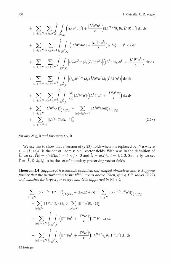
‖Lj∂µ�u(t, · )‖22 (2.28)
for any N ≥ 0 and for every t > 0.
We use this to show that a version of (2.23) holds when u is replaced by �µu where� = {L,�, ∂} is the set of “admissible” vector fields. With η as in the definition ofL̃, we set �̃ij = η(x)�ij, 1 ≤ i < j ≤ 3 and ∂̃i = η(x)∂i, i = 1, 2, 3. Similarly, we set�̃ = {L̃, �̃, ∂̃i, ∂t} to be the set of boundary-preserving vector fields.
Theorem 2.4 Suppose K is a smooth, bounded, star-shaped obstacle as above. Supposefurther that the perturbation terms hIJ,αβ are as above. Then, if u ∈ C∞ solves (2.22)and vanishes for large x for every t and G is supported in |x| < 2,
∑
|µ|≤N
‖〈x〉−1/2−�µu′‖2L2
t L2x(St)
+ (log(2 + t))−1∑
|µ|≤N
‖〈x〉−1/2�µu′‖2L2
t L2x(St)
+∑
|µ|≤N
‖�µu′(t, · )‖2 �∑
|µ|≤N
‖�µu′(0, · )‖22
+∑
|µ|,|ν|≤N
t∫
0
∫
R3\K
(|�µ∂uI | + |�µuI |
r
)|�νFI | dx ds
+∑
|µ|,|ν|≤N
t∫
0
∫
R3\K
(|�µ∂uI | + |�µuI |
r
)|[hIJ,γ δ∂γ ∂δ ,�ν]uJ| dx ds
Global existence of null-form wave equations in exterior domains 535
+∑
|µ|≤N,|ν|≤N−1
t∫
0
∫
R3\K
(|�µ∂uI | + |�µuI |
r
)|�ν(�u)I | dx ds
+∑
|µ|,|ν|≤N
t∫
0
∫
R3\K|(∂γ hIJ,γ δ)∂δ(�
µuJ)|(|�ν∂uI | + |�νuI |
r
)dx ds
+∑
|µ|,|ν|≤N
t∫
0
∫
R3\K
∣∣∣(∂t,rhIJ,γ δ)∂γ (�
µuJ)∂δ(�νuI)
∣∣∣ dx ds
+∑
|µ|+|σ |≤N|ν|≤N
t∫
0
∫
R3\K∩{|x|<1}|�σh||�µu′|
(|�νu′| + |�νu|
r
)dx ds
+∑
|µ|,|ν|≤N
t∫
0
∫
R3\K
|h|〈x〉 |�
µu′|(|�νu′| + |�νu|
r
)dx ds +
∑
|µ|≤N
‖�µG‖2L2
t L2x(St)
+∑
|µ|≤N−1
‖�µ�u‖2L2
t L2x(St)
+∑
|µ|≤N−1
‖�µ�u(t, · )‖22 (2.29)
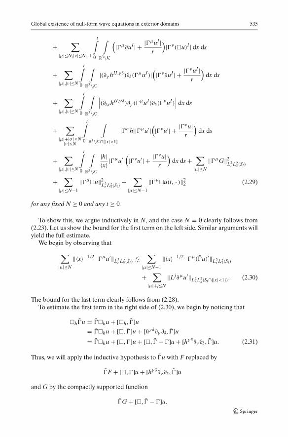
for any fixed N ≥ 0 and any t ≥ 0.
To show this, we argue inductively in N, and the case N = 0 clearly follows from(2.23). Let us show the bound for the first term on the left side. Similar arguments willyield the full estimate.
We begin by observing that
∑
|µ|≤N
‖〈x〉−1/2−�µu′‖L2t L2
x(St)�
∑
|µ|≤N−1
‖〈x〉−1/2−�µ(�̃u)′‖L2t L2
x(St)
+∑
|µ|+j≤N
‖Lj∂µu′‖L2t L2
x(St∩{|x|<1}). (2.30)
The bound for the last term clearly follows from (2.28).To estimate the first term in the right side of (2.30), we begin by noticing that
�h�̃u = �̃�hu + [�h, �̃]u= �̃�hu + [�, �̃]u + [hγ δ∂γ ∂δ , �̃]u= �̃�hu + [�,�]u + [�, �̃ − �]u + [hγ δ∂γ ∂δ , �̃]u. (2.31)
Thus, we will apply the inductive hypothesis to �̃u with F replaced by
�̃F + [�,�]u + [hγ δ∂γ ∂δ , �̃]u
and G by the compactly supported function
�̃G + [�, �̃ − �]u.
536 J. Metcalfe, C. D. Sogge
It follows that the first term in the right side of (2.30) is dominated by the right sideof (2.29) plus
∑
|µ|+j≤N
‖Lj∂µu′‖2L2
t L2x(St∩{|x|<1})
since the coefficients of Z are O(1) in {|x| < 1}. Thus, another application of (2.28)yields the desired estimate.
3 Decay estimates
Classically, the necessary decay to prove long-time existence is afforded to us by theKlainerman-Sobolev inequalities (see [13]; see also [6],[27]). These inequalities, how-ever, require the use of the Lorentz rotations which does not seem permissible inthe current setting. In order to get around this, we will rely on decay in |x| (whichmeshes well with the KSS estimates from the previous section) obtained by a weightedSobolev inequality and decay in t − |x| that follows from (variants of) estimates ofKlainerman and Sideris [15].
3.1 Null form estimates
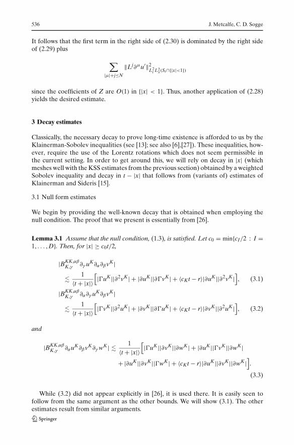
We begin by providing the well-known decay that is obtained when employing thenull condition. The proof that we present is essentially from [26].
Lemma 3.1 Assume that the null condition, (1.3), is satisfied. Let c0 = min{cI/2 : I =1, . . . , D}. Then, for |x| ≥ c0t/2,
|BKK,αβK,γ ∂γ uK∂α∂βvK|
�1
〈t + |x|〉[|�uK||∂2vK| + |∂uK||∂�vK| + 〈cKt − r〉|∂uK||∂2vK|
], (3.1)
|BKK,αβK,γ ∂α∂γ uK∂βvK|
�1
〈t + |x|〉[|�vK||∂2uK| + |∂vK||∂�uK| + 〈cKt − r〉|∂vK||∂2uK|
], (3.2)
and
|BKK,αβK,γ ∂αuK∂βvK∂γwK| �
1〈t + |x|〉
[|�uK||∂vK||∂wK| + |∂uK||�vK||∂wK|
+ |∂uK||∂vK||�wK| + 〈cKt − r〉|∂uK||∂vK||∂wK|].
(3.3)
While (3.2) did not appear explicitly in [26], it is used there. It is easily seen tofollow from the same argument as the other bounds. We will show (3.1). The otherestimates result from similar arguments.
Global existence of null-form wave equations in exterior domains 537
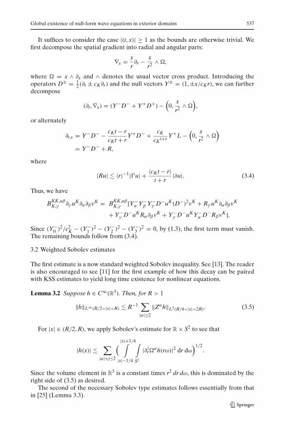
It suffices to consider the case |(t, x)| ≥ 1 as the bounds are otherwise trivial. Wefirst decompose the spatial gradient into radial and angular parts:
∇x = xr∂r − x
r2 ∧�,
where � = x ∧ ∂x and ∧ denotes the usual vector cross product. Introducing theoperators D± = 1
2 (∂t ± cK∂r) and the null vectors Y± = (1, ±x/cKr), we can furtherdecompose
(∂t, ∇x) = (Y−D− + Y+D+)−(
0,xr2 ∧�
),
or alternately
∂t,x = Y−D− − cKt − rcKt + r
Y+D− + cK
cKt+r Y+L −
(0,
xr2 ∧�
)
= Y−D− + R,
where
|Ru| � 〈r〉−1|�u| + 〈cKt − r〉t + r
|∂u|. (3.4)
Thus, we have
BKK,αβK,γ ∂γ uK∂α∂βvK = BKK,αβ
K,γ [Y−α Y−
β Y−γ D−uK(D−)2vK + Rγ uK∂α∂βvK
+ Y−γ D−uKRα∂βvK + Y−
γ D−uKY−α D−RβvK].
Since (Y−0 )
2/c2K − (Y−
1 )2 − (Y−
2 )2 − (Y−
3 )2 = 0, by (1.3), the first term must vanish.
The remaining bounds follow from (3.4).
3.2 Weighted Sobolev estimates
The first estimate is a now standard weighted Sobolev inequality. See [13]. The readeris also encouraged to see [11] for the first example of how this decay can be pairedwith KSS estimates to yield long time existence for nonlinear equations.
Lemma 3.2 Suppose h ∈ C∞(R3). Then, for R > 1
‖h‖L∞(R/2<|x|<R) � R−1∑
|α|≤2
‖Zαh‖L2(R/4<|x|<2R). (3.5)
For |x| ∈ (R/2, R), we apply Sobolev’s estimate for R × S2 to see that
|h(x)| �∑
|α|+j≤2
(|x|+1/4∫
|x|−1/4
∫
S2
|∂ jr�
αh(rω)|2 dr dω)1/2
.
Since the volume element in R3 is a constant times r2 dr dω, this is dominated by the
right side of (3.5) as desired.The second of the necessary Sobolev type estimates follows essentially from that
in [25] (Lemma 3.3).
538 J. Metcalfe, C. D. Sogge
Lemma 3.3 Let u ∈ C∞(R3\K) and suppose that u vanishes on ∂K and for large x forevery t. Then,
r1/2|u(t, x)| �∑
|µ|≤1
‖Zµu′(t, · )‖2. (3.6)
Moreover,
r1/2∑
|ν|≤N
|�νu(t, x)| �∑
|ν|≤N+1
‖�νu′(t, · )‖2 (3.7)
for any N ≥ 0.
We first note that the Dirichlet boundary condition allows us to control u locally byu′. Thus, over |x| ≤ 1, the result follows trivially from the standard Sobolev estimates.
In the remaining region, |x| ≥ 1, (3.6) is a consequence of the arguments in [25]. Wewrite x = rω where ω ∈ S2 (and dω denotes the surface measure of this unit sphere).We begin by noting that
r2|u(t, x)|4 �∑
|µ|≤1
r2‖�µu(t, r · )‖4L4(S2)
follows from a basic Sobolev estimate. By the fundamental theorem of calculus,Hölder’s inequality, and the standard Sobolev estimate ‖h‖6 � ‖∇h‖2, it followsthat
r2∫
S2
|v(t, rω)|4 dω � r2
∞∫
r
∫
S2
|∂rv(ρω)||v(ρω)|3 dρ dω
� ‖∂rv(t, · )‖2‖v(t, · )‖36 � ‖∇xv(t, · )‖4
2
which yields (3.6) when v is replaced by �µu.When |x| ≥ 1, (3.7) follows from the same argument as that for (3.6). Since the
coefficients of Z are O(1) for |x| ≤ 1, it only remains to show that∑
|ν|≤N
|Lνu(t, x)| �∑
|ν|≤N+1
‖�νu′(t, · )‖2, |x| ≤ 1. (3.8)
By Sobolev’s lemma, we have that for |x| ≤ 1,∑
|ν|≤N
|Lνu(t, x)| �∑
|ν|≤N+1
‖�νu′(t, · )‖2 +∑
|ν|≤N
‖Lνu(t, · )‖L2({|x|<2}).
The last term in the right side is
�∑
|ν|≤N
‖(t∂t)νu(t, · )‖L2({|x|<2}) +
∑
|ν|≤N−1
‖Lνu′(t, · )‖L2({|x|<2}).
Since ∂t preserves the Dirichlet boundary conditions, it follows from the FundamentalTheorem of Calculus that the former term is
�∑
|ν|≤N
‖(t∂t)νu′(t, · )‖L2({|x|<2}) �
∑
|ν|+|µ|≤N
‖Lν∂µu′(t, · )‖L2({|x|<2})
which completes the proof of (3.7).
Global existence of null-form wave equations in exterior domains 539
3.3 Klainerman-Sideris estimates
We finally present some estimates from [15] and some consequences of these esti-mates. These estimates are the ones that provide any required decay in the timevariable t.
We begin with the following basic estimate from [15],
〈cKt − r〉(|∂t∂uK| + |�uK|
)�
∑
|µ|≤1
|�µu′| + 〈t + r〉|�u|. (3.9)
Moreover, using integration by parts, it was shown that
‖〈cKt − r〉∂2vK(t, · )‖2 �∑
|µ|≤1
‖�µv′(t, · )‖2 + ‖〈t + r〉�v(t, · )‖2 (3.10)
when there is no boundary. Moreover, if one applies the boundaryless analog of (3.6)to 〈cKt − r〉∂vK and uses (3.10), the following is obtained,
r1/2〈cKt − r〉|∂vK(t, x)| �∑
|µ|≤2
‖�µv′(t, · )‖2 +∑
|µ|≤1
‖〈t + r〉�µ�v(t, · )‖2, (3.11)
which first appeared in Hidano and Yokoyama [5].When there is a boundary, the integration by parts argument in [15] does not yield
(3.10). We will, however, require analogous estimates. The first three are from [19].The first follows from applying (3.10) to η(x)u(t, x) where η is a smooth cutoff thatvanishes for |x| ≤ 1 and is identically one when |x| ≥ 3/2.
∑
|µ|≤N
‖〈cKt − r〉�µ∂2uK(t, · )‖2 �∑
|µ|≤N+1
‖�µu′(t, · )‖2
+∑
|µ|≤N
‖〈t + r〉�µ�u(t, · )‖2 + t∑
|µ|≤N
‖�µu′(t, · )‖L2({|x|<1}). (3.12)
Moreover, by combining (3.5), (3.12), and elliptic regularity (cf. [19]), one obtains
r〈cKt − r〉∑
|µ|≤N
|�µ∂2uK| �∑
|µ|≤N+3
‖�µu′(t, · )‖2
+∑
|µ|≤N+2
‖〈t + r〉�µ�u(t, · )‖2 + t∑
|µ|≤N
‖�µu′(t, · )‖L2({|x|<1}). (3.13)
Finally, by applying (3.6) to the cutoff solution and using (3.12), we can obtain thefollowing analog of the estimate from [5].
r1/2〈ckt − r〉∑
|µ|≤N
|�µ∂uK| �∑
|µ|≤N+2
‖�µu′(t, · )‖2 +∑
|µ|≤N+1
‖〈t + r〉�µ�u(t, · )‖2
+ t∑
|µ|≤N
‖�µu′(t, · )‖L2(|x|<1). (3.14)
540 J. Metcalfe, C. D. Sogge
As in [21], in a region |x| ≥ (c0/2)t, the boundary terms are no longer required. Inparticular, we have
∑
|µ|≤N
‖〈cKt − r〉∂2�µuK(t, · )‖L2(|x|≥c0t/2) �∑
|µ|≤N+1
‖�µu′(t, · )‖2
+∑
|µ|≤N
‖〈t + r〉�µ�u(t, · )‖L2(|x|≥c0t/4),
(3.15)
r〈cKt − r〉∑
|µ|≤N
|∂2�µuK(t, x)| �∑
|µ|≤N+3
‖�µu′(t, · )‖2
+∑
|µ|≤N+2
‖〈t + r〉�µ�u(t, · )‖L2(|x|≥c0t/4),
(3.16)
and
r1/2〈cKt − r〉∑
|µ|≤N
|∂�µuK(t, x)| �∑
|µ|≤N+2
‖�µu′(t, · )‖2
+∑
|µ|≤N+1
‖〈t + r〉�µ�u(t, · )‖L2(|x|≥c0t/4).
(3.17)
Indeed, we now fix η ∈ C∞(R3) satisfying η(x) ≡ 1, |x| > 1/2 and η(x) ≡ 0 for|x| < 1/4. We then set v(t, x) = η(x/(c0〈t〉))u(t, x) and apply (3.10) and (3.11).
4 Global existence
In this section, we prove our main result, Theorem 1.1. Here, we shall choose N = 30,but this is far from optimal. As in [26], the proof proceeds by examining a couplingbetween a low-order energy and a higher-order energy.
∑
|µ|≤20
(‖�µu′(t, · )‖2 + ‖〈x〉−5/8�µu′‖L2
t L2x(St)
)≤ Aε (4.1)
∑
|µ|≤30
(‖�µu′(t, · )‖2 + ‖〈x〉−5/8�µu′‖L2
t L2x(St)
)≤ Bε(1 + t)cε . (4.2)
Here, A is chosen to be 10 times greater than the square root of the implicit constantin (2.29). The exponent 5/8 was chosen to make the argument explicit. The sameargument would hold for sufficiently small ε for any exponent p with 1/2 < p < 3/4.
There are two steps required in order to complete the continuity argument:
(i.) Show (4.1) holds with A replaced by A/2,(ii.) Show that (4.2) follows from (4.1).
Throughout the remainder of the argument, we will be applying (2.29) with
hIJ,αβ = −BIJ,αβK,γ ∂γ uK
and F = G = 0.
Global existence of null-form wave equations in exterior domains 541
4.1 Preliminaries
Before beginning the proofs of (i.) and (ii.), we establish some preliminary estimates.These are shown assuming (4.1), and both are used to control terms that appear afterapplications of the decay estimates.
The first is a lower order version. We will establish:
∑
|µ|≤19
‖〈t + r〉�µ�u(t, · )‖2 � ε2 + tε∑
|µ|≤11
‖�µu′(t, · )‖L2(|x|<1). (4.3)
The left side of (4.3) is clearly controlled by
∑
|µ|≤11,|ν|≤20
‖〈t + r〉�µu′(t, · )�νu′(t, · )‖2.
When the norm is taken over |x| ≥ c0t/2, we can apply (3.5) and (4.1) to see that thisis O(ε2). When the norm is over |x| ≤ c0t/2, we apply (3.14) to see that this is
∑
|ν|≤20
‖�νu′(t, · )‖2
( ∑
|µ|≤14
‖�µu′(t, · )‖2 +∑
|µ|≤13
‖〈t + r〉�µ�u(t, · )‖2
+ t∑
|µ|≤11
‖�µu′(t, · )‖L2(|x|<1)
)� ε2 + ε
∑
|µ|≤13
‖〈t + r〉�µ�u(t, · )‖2
+ εt∑
|µ|≤11
‖�µu′(t, · )‖L2(|x|<1).
The last inequality follows from (4.1). Since the second term on the right can bebootstrapped if ε is sufficiently small, we see that this yields (4.3).
From this proof, it is easy to see that we also have
∑
|µ|≤19
‖〈t + r〉�µ�u(t, · )‖L2(|x|≥c0t/4) � ε2. (4.4)
We will additionally require the related higher order estimate
∑
|µ|≤29
‖〈t + r〉�µ�u(t, · )‖2 �(ε + t
∑
|µ|≤15
‖�µu′(t, · )‖L2(|x|<1)
) ∑
|ν|≤30
‖�νu′(t, · )‖2.
(4.5)
Plugging in our nonlinearity in the left, this is
�∑
|µ|≤30,|ν|≤15
‖〈t + r〉�µu′�νu′‖2.
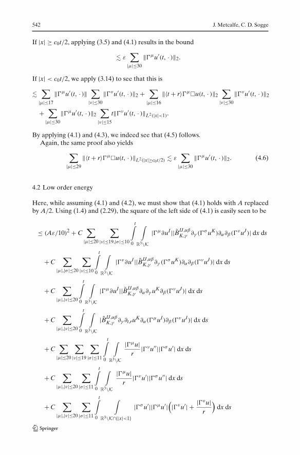
542 J. Metcalfe, C. D. Sogge
If |x| ≥ c0t/2, applying (3.5) and (4.1) results in the bound
� ε∑
|µ|≤30
‖�µu′(t, · )‖2.
If |x| < c0t/2, we apply (3.14) to see that this is
�∑
|µ|≤17
‖�µu′(t, · )‖∑
|ν|≤30
‖�νu′(t, · )‖2 +∑
|µ|≤16
‖〈t + r〉�µ�u(t, · )‖2∑
|ν|≤30
‖�νu′(t, · )‖2
+∑
|µ|≤30
‖�µu′(t, · )‖2∑
|ν|≤15
t‖�νu′(t, · )‖L2(|x|<1).
By applying (4.1) and (4.3), we indeed see that (4.5) follows.Again, the same proof also yields
∑
|µ|≤29
‖〈t + r〉�µ�u(t, · )‖L2(|x|≥c0t/2) � ε∑
|µ|≤30
‖�µu′(t, · )‖2. (4.6)
4.2 Low order energy
Here, while assuming (4.1) and (4.2), we must show that (4.1) holds with A replacedby A/2. Using (1.4) and (2.29), the square of the left side of (4.1) is easily seen to be
≤ (Aε/10)2 + C∑
|µ|≤20
∑
|ν|≤19,|σ |≤10
t∫
0
∫
R3\K|�µ∂uI ||B̃IJ,αβ
K,γ ∂γ (�σuK)∂α∂β(�
νuJ)| dx ds
+ C∑
|µ|,|σ |≤20
∑
|ν|≤10
t∫
0
∫
R3\K|�ν∂uI ||B̃IJ,αβ
K,γ ∂γ (�σuK)∂α∂β(�
νuJ)| dx ds
+ C∑
|µ|,|ν|≤20
t∫
0
∫
R3\K|�µ∂uI ||B̃IJ,αβ
K,γ ∂α∂γ uK∂β(�νuJ)| dx ds
+ C∑
|µ|,|ν|≤20
t∫
0
∫
R3\K|B̃IJ,αβ
K,γ ∂γ ∂t,ruK∂α(�µuI)∂β(�
νuJ)| dx ds
+ C∑
|µ|≤20
∑
|ν|≤19
∑
|σ |≤11
t∫
0
∫
R3\K
|�µu|r
|�νu′′||�σu′| dx ds
+ C∑
|µ|,|ν|≤20
∑
|σ |≤11
t∫
0
∫
R3\K
|�µu|r
|�νu′||�σu′′| dx ds
+ C∑
|µ|,|ν|≤20
∑
|σ |≤11
t∫
0
∫
R3\K∩{|x|<1}|�σu′||�µu′|
(|�νu′| + |�νu|
r
)dx ds
Global existence of null-form wave equations in exterior domains 543
+ C∑
|µ|,|ν|≤20
t∫
0
∫
R3\K
1〈x〉 |u
′||�µu′|(|�νu′| + |�νu|
r
)dx ds
+ C∑
|µ|≤20
∑
|ν|≤11
‖|�νu′| |�µu′|‖2L2
t L2x(St)
+ C∑
|µ≤20
∑
|ν|≤11
‖|�νu′(t, · )| |�µu′(t, · )|‖22.
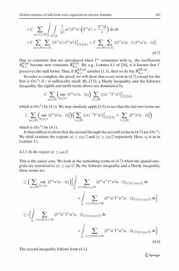
(4.7)
Due to constants that are introduced when �µ commutes with ∂α , the coefficientsBIJ,αβ
K,γ become new constants B̃IJ,αβK,γ . By, e.g., Lemma 4.1 of [26], it is known that �
preserves the null forms. Thus, if BKK,αβK,γ satisfies (1.3), then so do the B̃KK,αβ
K,γ .In order to complete the proof, we will show that every term in (4.7) except for the
first is O(ε3) if ε is sufficiently small. By (3.5), a Hardy inequality, and the Schwarzinequality, the eighth and ninth terms above are dominated by
C∑
|µ|≤20
(sup
0≤s≤t‖�µu′(s, · )‖2
) ∑
|ν|≤20
‖〈x〉−1�νu′‖2L2
t L2x(St)
which is O(ε3) by (4.1). We may similarly apply (3.5) to see that the last two terms are
�∑
|µ|≤20
(sup
0≤s≤t‖�µu′(s, · )‖2
2
)( ∑
|ν|≤20
‖〈x〉−1�νu′‖2L2
t L2x(St)
+∑
|ν|≤20
‖�νu′(t, · )‖22
)
which is O(ε4) by (4.1).It thus suffices to show that the second through the seventh terms in (4.7) are O(ε3).
We shall examine the regions |x| ≤ c0s/2 and |x| ≥ c0s/2 separately. Here, c0 is as inLemma 3.1.
4.2.1 In the region |x| ≤ c0s/2
This is the easier case. We look at the remaining terms in (4.7) when the spatial inte-grals are restricted to |x| ≤ c0s/2. By the Schwarz inequality and a Hardy inequality,these terms are
�( ∑
|µ|≤20
sup0≤s≤t
‖�µu′(s, · )‖2
)[t∫
0
∑
|ν|≤20,|σ |≤10
‖�σu′′ �νu′(s, · )‖L2(|x|≤c0s/2) ds
+t∫
0
∑
|ν|≤19,|σ |≤10
‖�σu′ �νu′′(s, · )‖L2(|x|≤c0s/2) ds]
� ε[
t∫
0
∑
|ν|≤20,|σ |≤10
‖�σu′′ �νu′(s, · )‖L2(|x|≤c0s/2) ds
+t∫
0
∑
|ν|≤19,|σ |≤10
‖�σu′ �νu′′(s, · )‖L2(|x|≤c0s/2) ds].
(4.8)
The second inequality follows from (4.1).
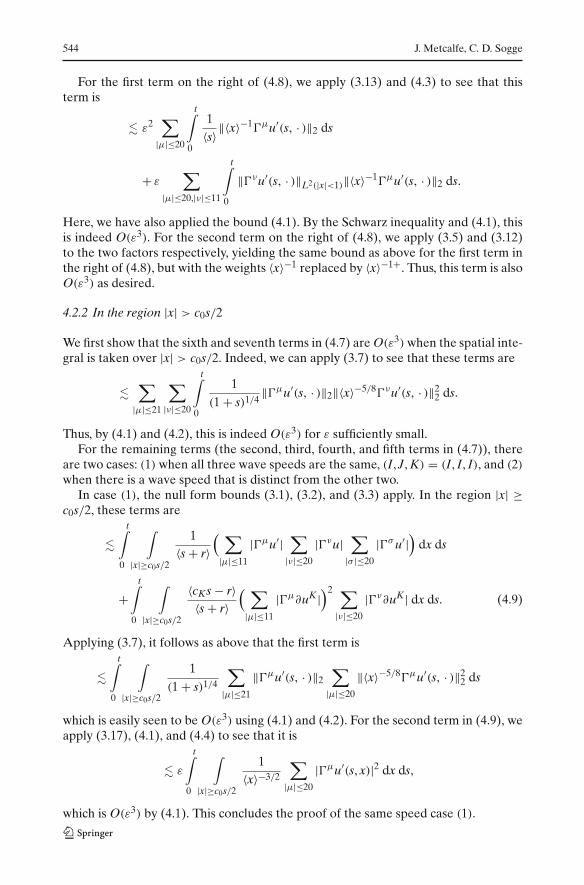
544 J. Metcalfe, C. D. Sogge
For the first term on the right of (4.8), we apply (3.13) and (4.3) to see that thisterm is
� ε2∑
|µ|≤20
t∫
0
1〈s〉‖〈x〉−1�µu′(s, · )‖2 ds
+ ε∑
|µ|≤20,|ν|≤11
t∫
0
‖�νu′(s, · )‖L2(|x|<1)‖〈x〉−1�µu′(s, · )‖2 ds.
Here, we have also applied the bound (4.1). By the Schwarz inequality and (4.1), thisis indeed O(ε3). For the second term on the right of (4.8), we apply (3.5) and (3.12)to the two factors respectively, yielding the same bound as above for the first term inthe right of (4.8), but with the weights 〈x〉−1 replaced by 〈x〉−1+. Thus, this term is alsoO(ε3) as desired.
4.2.2 In the region |x| > c0s/2
We first show that the sixth and seventh terms in (4.7) are O(ε3)when the spatial inte-gral is taken over |x| > c0s/2. Indeed, we can apply (3.7) to see that these terms are
�∑
|µ|≤21
∑
|ν|≤20
t∫
0
1(1 + s)1/4
‖�µu′(s, · )‖2‖〈x〉−5/8�νu′(s, · )‖22 ds.
Thus, by (4.1) and (4.2), this is indeed O(ε3) for ε sufficiently small.For the remaining terms (the second, third, fourth, and fifth terms in (4.7)), there
are two cases: (1) when all three wave speeds are the same, (I, J, K) = (I, I, I), and (2)when there is a wave speed that is distinct from the other two.
In case (1), the null form bounds (3.1), (3.2), and (3.3) apply. In the region |x| ≥c0s/2, these terms are
�t∫
0
∫
|x|≥c0s/2
1〈s + r〉
( ∑
|µ|≤11
|�µu′|∑
|ν|≤20
|�νu|∑
|σ |≤20
|�σu′|)
dx ds
+t∫
0
∫
|x|≥c0s/2
〈cKs − r〉〈s + r〉
( ∑
|µ|≤11
|�µ∂uK|)2 ∑
|ν|≤20
|�ν∂uK| dx ds. (4.9)
Applying (3.7), it follows as above that the first term is
�t∫
0
∫
|x|≥c0s/2
1(1 + s)1/4
∑
|µ|≤21
‖�µu′(s, · )‖2∑
|µ|≤20
‖〈x〉−5/8�µu′(s, · )‖22 ds
which is easily seen to be O(ε3) using (4.1) and (4.2). For the second term in (4.9), weapply (3.17), (4.1), and (4.4) to see that it is
� ε
t∫
0
∫
|x|≥c0s/2
1〈x〉−3/2
∑
|µ|≤20
|�µu′(s, x)|2 dx ds,
which is O(ε3) by (4.1). This concludes the proof of the same speed case (1).
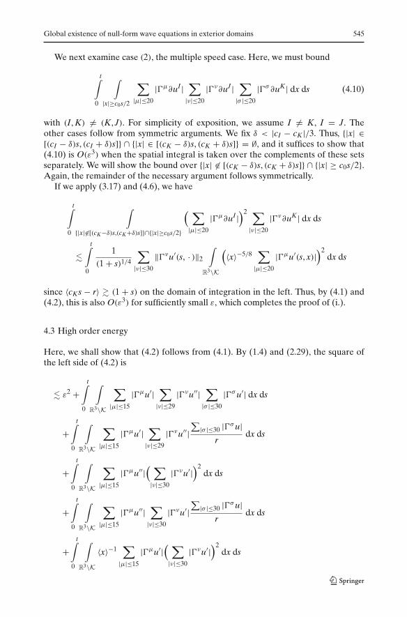
Global existence of null-form wave equations in exterior domains 545
We next examine case (2), the multiple speed case. Here, we must bound
t∫
0
∫
|x|≥c0s/2
∑
|µ|≤20
|�µ∂uI |∑
|ν|≤20
|�ν∂uJ|∑
|σ |≤20
|�σ ∂uK| dx ds (4.10)
with (I, K) �= (K, J). For simplicity of exposition, we assume I �= K, I = J. Theother cases follow from symmetric arguments. We fix δ < |cI − cK|/3. Thus, {|x| ∈[(cI − δ)s, (cI + δ)s]} ∩ {|x| ∈ [(cK − δ)s, (cK + δ)s]} = ∅, and it suffices to show that(4.10) is O(ε3) when the spatial integral is taken over the complements of these setsseparately. We will show the bound over {|x| �∈ [(cK − δ)s, (cK + δ)s]} ∩ {|x| ≥ c0s/2}.Again, the remainder of the necessary argument follows symmetrically.
If we apply (3.17) and (4.6), we have
t∫
0
∫
{|x|�∈[(cK−δ)s,(cK+δ)s]}∩{|x|≥c0s/2}
( ∑
|µ|≤20
|�µ∂uI |)2 ∑
|ν|≤20
|�ν∂uK| dx ds
�t∫
0
1(1 + s)1/4
∑
|ν|≤30
‖�νu′(s, · )‖2
∫
R3\K
(〈x〉−5/8
∑
|µ|≤20
|�µu′(s, x)|)2
dx ds
since 〈cKs − r〉 � (1 + s) on the domain of integration in the left. Thus, by (4.1) and(4.2), this is also O(ε3) for sufficiently small ε, which completes the proof of (i.).
4.3 High order energy
Here, we shall show that (4.2) follows from (4.1). By (1.4) and (2.29), the square ofthe left side of (4.2) is
� ε2 +t∫
0
∫
R3\K
∑
|µ|≤15
|�µu′|∑
|ν|≤29
|�νu′′|∑
|σ |≤30
|�σu′| dx ds
+t∫
0
∫
R3\K
∑
|µ|≤15
|�µu′|∑
|ν|≤29
|�νu′′|∑
|σ |≤30 |�σu|r
dx ds
+t∫
0
∫
R3\K
∑
|µ|≤15
|�µu′′|( ∑
|ν|≤30
|�νu′|)2
dx ds
+t∫
0
∫
R3\K
∑
|µ|≤15
|�µu′′|∑
|ν|≤30
|�νu′|∑
|σ |≤30 |�σu|r
dx ds
+t∫
0
∫
R3\K〈x〉−1
∑
|µ|≤15
|�µu′|( ∑
|ν|≤30
|�νu′|)2
dx ds
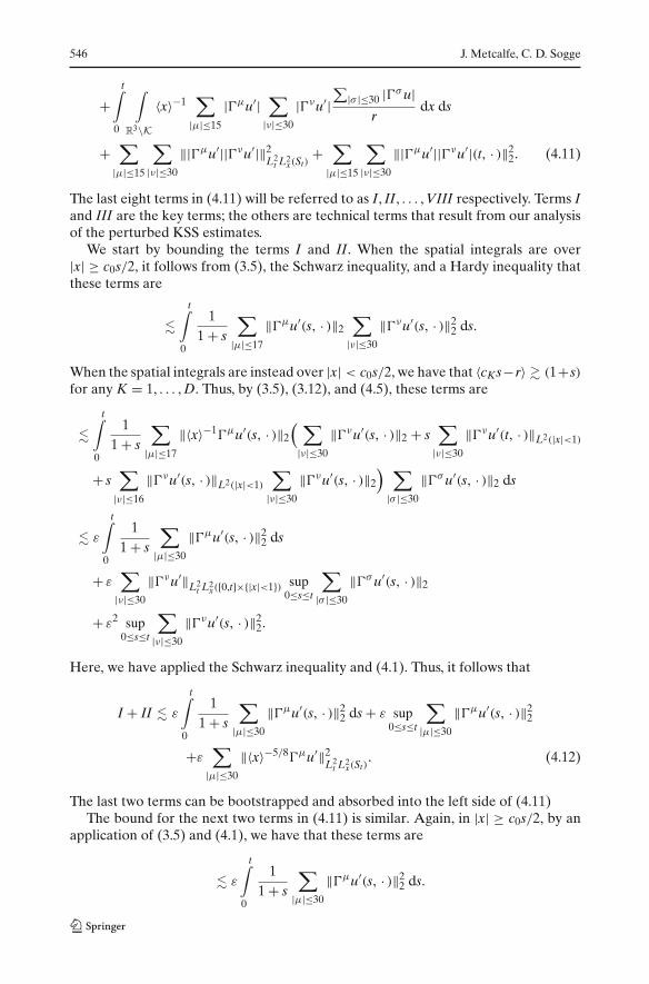
546 J. Metcalfe, C. D. Sogge
+t∫
0
∫
R3\K〈x〉−1
∑
|µ|≤15
|�µu′|∑
|ν|≤30
|�νu′|∑
|σ |≤30 |�σu|r
dx ds
+∑
|µ|≤15
∑
|ν|≤30
‖|�µu′||�νu′|‖2L2
t L2x(St)
+∑
|µ|≤15
∑
|ν|≤30
‖|�µu′||�νu′|(t, · )‖22. (4.11)
The last eight terms in (4.11) will be referred to as I, II, . . . , VIII respectively. Terms Iand III are the key terms; the others are technical terms that result from our analysisof the perturbed KSS estimates.
We start by bounding the terms I and II. When the spatial integrals are over|x| ≥ c0s/2, it follows from (3.5), the Schwarz inequality, and a Hardy inequality thatthese terms are
�t∫
0
11 + s
∑
|µ|≤17
‖�µu′(s, · )‖2∑
|ν|≤30
‖�νu′(s, · )‖22 ds.
When the spatial integrals are instead over |x| < c0s/2, we have that 〈cKs−r〉 � (1+s)for any K = 1, . . . , D. Thus, by (3.5), (3.12), and (4.5), these terms are
�t∫
0
11 + s
∑
|µ|≤17
‖〈x〉−1�µu′(s, · )‖2
( ∑
|ν|≤30
‖�νu′(s, · )‖2 + s∑
|ν|≤30
‖�νu′(t, · )‖L2(|x|<1)
+ s∑
|ν|≤16
‖�νu′(s, · )‖L2(|x|<1)
∑
|ν|≤30
‖�νu′(s, · )‖2
) ∑
|σ |≤30
‖�σu′(s, · )‖2 ds
� ε
t∫
0
11 + s
∑
|µ|≤30
‖�µu′(s, · )‖22 ds
+ ε∑
|ν|≤30
‖�νu′‖L2t L2
x([0,t]×{|x|<1}) sup0≤s≤t
∑
|σ |≤30
‖�σu′(s, · )‖2
+ ε2 sup0≤s≤t
∑
|ν|≤30
‖�νu′(s, · )‖22.
Here, we have applied the Schwarz inequality and (4.1). Thus, it follows that
I + II � ε
t∫
0
11 + s
∑
|µ|≤30
‖�µu′(s, · )‖22 ds + ε sup
0≤s≤t
∑
|µ|≤30
‖�µu′(s, · )‖22
+ε∑
|µ|≤30
‖〈x〉−5/8�µu′‖2L2
t L2x(St)
. (4.12)
The last two terms can be bootstrapped and absorbed into the left side of (4.11)The bound for the next two terms in (4.11) is similar. Again, in |x| ≥ c0s/2, by an
application of (3.5) and (4.1), we have that these terms are
� ε
t∫
0
11 + s
∑
|µ|≤30
‖�µu′(s, · )‖22 ds.
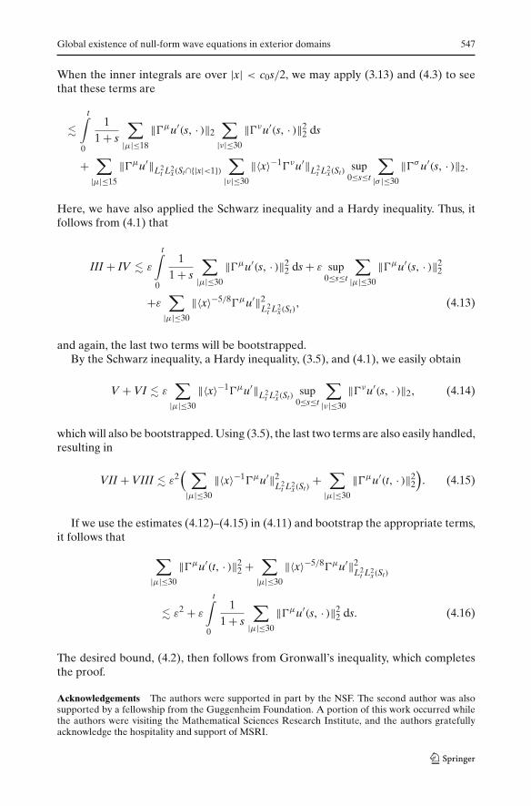
Global existence of null-form wave equations in exterior domains 547
When the inner integrals are over |x| < c0s/2, we may apply (3.13) and (4.3) to seethat these terms are
�t∫
0
11 + s
∑
|µ|≤18
‖�µu′(s, · )‖2∑
|ν|≤30
‖�νu′(s, · )‖22 ds
+∑
|µ|≤15
‖�µu′‖L2t L2
x(St∩{|x|<1})∑
|ν|≤30
‖〈x〉−1�νu′‖L2t L2
x(St)sup
0≤s≤t
∑
|σ |≤30
‖�σu′(s, · )‖2.
Here, we have also applied the Schwarz inequality and a Hardy inequality. Thus, itfollows from (4.1) that
III + IV � ε
t∫
0
11 + s
∑
|µ|≤30
‖�µu′(s, · )‖22 ds + ε sup
0≤s≤t
∑
|µ|≤30
‖�µu′(s, · )‖22
+ε∑
|µ|≤30
‖〈x〉−5/8�µu′‖2L2
t L2x(St)
, (4.13)
and again, the last two terms will be bootstrapped.By the Schwarz inequality, a Hardy inequality, (3.5), and (4.1), we easily obtain
V + VI � ε∑
|µ|≤30
‖〈x〉−1�µu′‖L2t L2
x(St)sup
0≤s≤t
∑
|ν|≤30
‖�νu′(s, · )‖2, (4.14)
which will also be bootstrapped. Using (3.5), the last two terms are also easily handled,resulting in
VII + VIII � ε2( ∑
|µ|≤30
‖〈x〉−1�µu′‖2L2
t L2x(St)
+∑
|µ|≤30
‖�µu′(t, · )‖22
). (4.15)
If we use the estimates (4.12)–(4.15) in (4.11) and bootstrap the appropriate terms,it follows that
∑
|µ|≤30
‖�µu′(t, · )‖22 +
∑
|µ|≤30
‖〈x〉−5/8�µu′‖2L2
t L2x(St)
� ε2 + ε
t∫
0
11 + s
∑
|µ|≤30
‖�µu′(s, · )‖22 ds. (4.16)
The desired bound, (4.2), then follows from Gronwall’s inequality, which completesthe proof.
Acknowledgements The authors were supported in part by the NSF. The second author was alsosupported by a fellowship from the Guggenheim Foundation. A portion of this work occurred whilethe authors were visiting the Mathematical Sciences Research Institute, and the authors gratefullyacknowledge the hospitality and support of MSRI.
548 J. Metcalfe, C. D. Sogge
References
1. Agemi, R., Yokoyama, K.: The null condition and global existence of solutions to systems of waveequations with different speeds. Adv. Nonlinear Partial Differ. Equ. Stochastics, 43–86 (1998)
2. Alinhac, S.: On the Morawetz/KSS inequality for the wave equation on a curved background.preprint (2005)
3. Christodoulou, D.: Global solutions of nonlinear hyperbolic equations for small initialdata. Comm. Pure Appl. Math. 39, 267–282 (1986)
4. Hidano, K.: An elementary proof of global or almost global existence for quasi-linear waveequations. Tohoku Math. J. 56, 271–287 (2004)
5. Hidano, K., Yokoyama, K.: A remark on the almost global existence theorems of Keel, Smith,and Sogge. Funkcial. Ekvac. 48, 1–34 (2005)
6. Hörmander, L.: Lectures on Nonlinear Hyperbolic Equations. Springer, Heidelberg New York,Berlin (1997)
7. Katayama, S.: Global existence for a class of systems of nonlinear wave equations in three spacedimensions. Chinese Ann. Math. Ser. B, 25, 463–482 (2004)
8. Katayama, S.: Global existence for systems of wave equations with nonresonant nonlinearitiesand null forms. J. Differ. Equ. 209, 140–171 (2005)
9. Katayama, S.: A remark on systems of nonlinear wave equations with different propagationspeeds. preprint (2003).
10. Keel, M., Smith, H., Sogge, C.D.: Global existence for a quasilinear wave equation outside ofstar-shaped domains. J. Funct. Anal. 189, 155–226 (2002)
11. Keel, M., Smith, H., Sogge, C.D.: Almost global existence for some semilinear wave equa-tions. J. D’Analyse 87, 265–279 (2002)
12. Keel, M., Smith, H., Sogge, C.D.: Almost global existence for quasilinear wave equations in threespace dimensions. J. Am. Math. Soc. 17, 109–153 (2004)
13. Klainerman, S.: Uniform decay estimates and the Lorentz invariance of the classical wave equa-tion. Commun. Pure Appl. Math. 38, 321–332 (1985)
14. Klainerman, S.: The null condition and global existence to nonlinear wave equations. Lect. Appl.Math. 23, 293–326 (1986)
15. Klainerman, S., Sideris, T.: On almost global existence for nonrelativistic wave equations in3d. Commun. Pure Appl. Math. 49, 307–321 (1996)
16. Kubota, K., Yokoyama, K.: Global existences of classical solutions to systems of nonlinear waveequations with different speeds of propagation. Jpn. J. Math. 27, 113–202 (2001)
17. Lax, P.D., Morawetz, C.S., Phillips, R.S.: Exponential decay of solutions of the wave equation inthe exterior of a star-shaped obstacle. Commun. Pure Appl. Math. 16, 477–486 (1963)
18. Metcalfe, J.: Global existence for semilinear wave equations exterior to nontrapping obstacles.Houston J. Math. 30, 259–281 (2004)
19. Metcalfe, J., Nakamura, M., Sogge, C.D.: Global existence of solutions to multiple speed systemsof quasilinear wave equations in exterior domains. Forum. Math. 17, 133–168 (2005)
20. Metcalfe, J., Nakamura, M., Sogge, C.D.: Global existence of quasilinear, nonrelativistic waveequations satisfying the null condition. Jpn. J. Math. 31, 391–472 (2005)
21. Metcalfe, J., Sogge, C.D.: Hyperbolic trapped rays and global existence of quasilinear waveequations. Invent. Math. 159, 75–117 (2005)
22. Metcalfe, J., Sogge, C.D.: Global existence for Dirichlet-wave equations with quadratic nonlin-earities in high dimensions. Math. Ann. (to appear)
23. Metcalfe, J., Sogge, C.D.: Long time existence of quasilinear wave equations exterior to star-shaped obstacles via energy methods. SIAM J. Math. Anal. 38, 188–209 (2006)
24. Morawetz, C.S.: The decay of solutions of the exterior initial-boundary problem for the waveequation. Commun. Pure Appl. Math. 14, 561–568 (1961)
25. Sideris, T.: Nonresonance and global existence of prestressed nonlinear elastic waves. Ann.Math. 151, 849–874 (2000)
26. Sideris, T., Tu, S.Y.: Global existence for systems of nonlinear wave equations in 3D with multiplespeeds. SIAM J. Math. Anal. 33, 477–488 (2001)
27. Sogge, C.D.: Lectures on Nonlinear Wave Equations. International Press, Cambridge (1995)28. Sogge, C.D.: Global existence for nonlinear wave equations with multiple speeds. In Harmonic
analysis, Mount Holyoke (South Hadley, 2001), pp. 353–366, Contemp. Math., 320, Amer. Math.Soc., Providence, RI, 2003.
29. Sterbenz, J.: Angular regularity and Strichartz estimates for the wave equation with an appendixby I. Rodnianski. Int. Math. Res. Notes 2005, 187–231.
Global existence of null-form wave equations in exterior domains 549
30. Strauss, W.A.: Dispersal of waves vanishing on the boundary of an exterior domain. Commun.Pure Appl. Math. 28, 265–278 (1975)
31. Yokoyama, K.: Global existence of classical solutions to systems of wave equations with criticalnonlinearity in three space dimensions. J. Math. Soc. Japan 52, 609–632 (2000)