Global evaluation of runoff from 10 state-of-the-art

Hydrol. Earth Syst. Sci., 21, 2881–2903, 2017https://doi.org/10.5194/hess-21-2881-2017© Author(s) 2017. This work is distributed underthe Creative Commons Attribution 3.0 License.

Global evaluation of runoff from 10 state-of-the-arthydrological modelsHylke E. Beck1,3, Albert I. J. M. van Dijk2, Ad de Roo3, Emanuel Dutra4,5, Gabriel Fink6, Rene Orth7, andJaap Schellekens8

1Civil and Environmental Engineering, Princeton University, Princeton, NJ, USA2Fenner School of Environment & Society, Australian National University (ANU), Canberra, Australia3European Commission, Joint Research Centre (JRC), Via Enrico Fermi 2749, 21027 Ispra (VA), Italy4European Centre for Medium-Range Weather Forecasts (ECMWF), Redding, UK5Instituto Dom Luiz, Faculdade de Ciências, Universidade de Lisboa, 1749-016 Lisbon, Portugal6Center for Environmental Systems Research (CESR), University of Kassel, Kassel, Germany7Institute for Atmospheric and Climate Science, ETH Zurich, Zurich, Switzerland8Inland Water Systems Unit, Deltares, Delft, the Netherlands

Correspondence to: Hylke E. Beck ([email protected])

Received: 13 March 2016 – Discussion started: 20 May 2016Revised: 6 April 2017 – Accepted: 29 April 2017 – Published: 12 June 2017

Abstract. Observed streamflow data from 966 medium sizedcatchments (1000–5000 km2) around the globe were used tocomprehensively evaluate the daily runoff estimates (1979–2012) of six global hydrological models (GHMs) and fourland surface models (LSMs) produced as part of tier-1 of theeartH2Observe project. The models were all driven by theWATCH Forcing Data ERA-Interim (WFDEI) meteorologi-cal dataset, but used different datasets for non-meteorologicinputs and were run at various spatial and temporal resolu-tions, although all data were re-sampled to a common 0.5◦

spatial and daily temporal resolution. For the evaluation, weused a broad range of performance metrics related to impor-tant aspects of the hydrograph. We found pronounced inter-model performance differences, underscoring the importanceof hydrological model uncertainty in addition to climate in-put uncertainty, for example in studies assessing the hydro-logical impacts of climate change. The uncalibrated GHMswere found to perform, on average, better than the uncali-brated LSMs in snow-dominated regions, while the ensemblemean was found to perform only slightly worse than the best(calibrated) model. The inclusion of less-accurate models didnot appreciably degrade the ensemble performance. Overall,we argue that more effort should be devoted on calibratingand regionalizing the parameters of macro-scale models. Wefurther found that, despite adjustments using gauge obser-

vations, the WFDEI precipitation data still contain substan-tial biases that propagate into the simulated runoff. The earlybias in the spring snowmelt peak exhibited by most modelsis probably primarily due to the widespread precipitation un-derestimation at high northern latitudes.

1 Introduction

Hydrological models are indispensable tools for many pur-poses including, but not limited to, (i) flood and drought fore-casting, (ii) water resources assessments, (iii) assessing thehydrological impacts of human activities, and (iv) increas-ing our understanding of the hydrological cycle. It is morethan 50 years since the first attempts at hydrological mod-eling (Linsley and Crawford, 1960; Rockwood, 1964; Sug-awara, 1967; Freeze and Harlan, 1969). Since then, a plethoraof conceptual, physically based, and stochastic hydrologicalmodels has been developed, each with its own assumptionsand characteristics (for non-exhaustive overviews; see Singh,1995; Singh and Frevert, 2002; Rosbjerg and Madsen, 2006;Trambauer et al., 2013; Sooda and Smakhtin, 2015; Bierkenset al., 2015; Kauffeldt et al., 2016). Because all hydrolog-ical models are inevitably imperfect representations of real-

Published by Copernicus Publications on behalf of the European Geosciences Union.

2882 H. E. Beck et al.: Evaluation of runoff from 10 hydrological models

ity, they produce highly uncertain estimates even if we wouldhave access to perfect meteorological data (Beven, 1989).

The quantification of these uncertainties using indepen-dent data sources is of critical importance to advance modeldevelopment, reject deficient model structures and parame-terizations, quantify model credibility, and ultimately bringsome order to the plethora of models (Klemeš, 1986; Wa-gener, 2003; Döll et al., 2015; Clark et al., 2015). Therehave been several collaborative research efforts focusing onthe intercomparison and verification of hydrological models.The earliest were coordinated by the World MeteorologicalOrganization (WMO, 1975, 1986, 1992). Other noteworthyinitiatives include the Model Parameter Estimation Experi-ment (MOPEX; Duan et al., 2006), the Global Soil WetnessProject (GSWP; Dirmeyer, 2011), the Water Model Inter-comparison Project (WaterMIP; Haddeland et al., 2011), andthe Global Energy and Water Exchanges (GEWEX) Land-Flux project (McCabe et al., 2016). These initiatives have ledto numerous multi-model evaluation studies focusing on suchhydrological variables as runoff (e.g., Gudmundsson et al.,2012a; Zhou et al., 2012), evaporation (e.g., Schlosser andGao, 2010; Jiménez et al., 2011; Miralles et al., 2015), soilmoisture (e.g., Guo et al., 2007; Xia et al., 2014), snow cover(e.g., Slater et al., 2001), and total water storage (Güntner,2008), among others.

One of the most useful variables for hydrological modelevaluation is runoff, since it reflects the integrated responseof a host of hydrological processes occurring in a catch-ment (Fekete et al., 2012) and because observations are read-ily available for many catchments across the globe (Hannahet al., 2011). Table 1 lists, to our knowledge, all macro-scale(i.e., continental to global scale) studies evaluating the runoffestimates of multiple models that have been published sofar. Out of these 20 studies, two focused on the contermi-nous USA, five focused on Europe, while 13 had a globalscope. However, many of these studies used observationsfrom a relatively small number (< 100) of large catchments(� 10000 km2). The use of a small number of basins limitsconfidence in the results and precludes a spatially detailedassessment, while the large size of the catchments makes itmore difficult to distinguish between deficiencies in the forc-ing, the (sub-)surface component, or the river routing com-ponent of the modeling chain. Moreover, a large number ofthe studies only evaluated monthly mean runoff, precludinganalysis of the shape of individual flow events, or used theNash and Sutcliffe (1970) efficiency (NSE), which has beencriticized in several previous studies for being overly sensi-tive to the timing and magnitude of peak flows (Schaefli andGupta, 2007; Jain and Sudheer, 2008). Furthermore, manystudies considered only a few hydrological models (≤ 5) orperformance metrics (≤ 2), limiting the insights that can begained.

As part of tier-1 of the eartH2Observe project, 10 state-of-the-art hydrological models were run globally at a daily timestep for the period 1979–2012 using the same forcing dataset,

in an effort to develop a global reanalysis of water resourcesthat supports efficient water management and decision mak-ing (Schellekens et al., 2016). Six of the models are globalhydrological models (GHMs) while four of the models areland surface models (LSMs). GHMs have traditionally beendesigned to simulate (sub-)surface water fluxes and storages,while LSMs have traditionally been designed to simulatethe soil–vegetation–atmosphere interactions within climatemodels (Haddeland et al., 2011; Bierkens, 2015). GHMs gen-erally represent hydrological processes in a more conceptualway, solve only the water balance, commonly operate at dailytime steps, and typically have a small number of soil lay-ers (≤ 3 in the current study) and a single snow layer. Con-versely, LSMs generally represent hydrological processes ina more physically based way, solve both the water and en-ergy balances, typically operate at (sub-)hourly time steps,and tend to have many soil and snow layers (4–11 and 1–12, respectively, in the current study; for more details on themodels, see Table 1 of Schellekens et al., 2016). The presentstudy aims to comprehensively evaluate the runoff estimatesof these 10 models across the globe in an effort to answer thefollowing pertinent research questions:

1. How well do the different models simulate runoff?

2. How well do the models perform in terms of long-termrunoff trends?

3. How do the results of the GHMs differ, if at all, fromthose of the LSMs?

4. Are calibration and regionalization important or evenessential?

5. What is the impact of the forcing data on the simulatedrunoff?

6. How valuable are multi-model ensembles for improvingrunoff estimates?

7. Do all models show the early bias in runoff timingin snow-dominated catchments previously documented(e.g., Zaitchik et al., 2010) and what is the cause?

We use daily streamflow observations during 1979–2012from a large, highly diverse, quality-controlled set ofmedium-sized catchments, which allows us to compare theperformance among different regions and climate types (An-dréassian et al., 2007; Stahl et al., 2011; Gupta et al., 2014).Moreover, we use a broad range of performance metrics, in-cluding runoff signatures (measures that quantify the hydro-graph shape such as runoff coefficient and baseflow index;Olden and Poff, 2003; Monk et al., 2007) that can be relatedto specific hydrological processes (Yilmaz et al., 2008).

Hydrol. Earth Syst. Sci., 21, 2881–2903, 2017 www.hydrol-earth-syst-sci.net/21/2881/2017/

H. E. Beck et al.: Evaluation of runoff from 10 hydrological models 2883

Table 1. Overview of, to the best of our knowledge, all macro-scale (continental to global) studies evaluating the runoff estimates of multiplemodels, sorted by region and then publication date. The present study has been added for the sake of completeness.

Study Region Number of Number of catchments (size range) Evaluation timescale(s)models

Lohmann et al. (2004) Cont. USA 4 1145 (23 to 10 000 km2) Daily, monthly, annual, long-termXia et al. (2012) Cont. USA 4 969 (23 to 1 353 280 km2) Daily, weekly, monthly, annual, long-termPrudhomme et al. (2011) Europe 3 579 (< 1000 km2) DailyGudmundsson et al. (2012a) Europe 9 426 (< 4000 km2) Daily, annual, long-termGudmundsson et al. (2012b) Europe 9 426 (< 4000 km2) Annual, long-termGreuell et al. (2015) Europe 5 46 (9948 to 658 340 km2) Daily, monthly, annual, long-termGudmundsson and Seneviratne (2015) Europe 10 426 (< 4000 km2) Monthly, annual, long-termMilly et al. (2005) Global 12 165 (> 50000 km2) Long-termDecharme and Douville (2006) Global 6 80 (100 000 to 4 758 000 km2) Daily, monthlyDecharme and Douville (2007) Global 6 80 (100 000 to 4 758 000 km2) MonthlyDecharme (2007) Global 2 80 (100 000 to 4 758 000 km2) MonthlyMateria et al. (2010) Global 13 30 (82 000 to 4 677 000 km2) MonthlyZaitchik et al. (2010) Global 4 66 (19 000 to 4 600 000 km2) Daily, annualHaddeland et al. (2011) Global 11 8 (650 000 to 4 600 000 km2) MonthlyZhou et al. (2012) Global 14 150 (not specified;� 10000 km2) AnnualVan Dijk et al. (2013b) Global 5 6192 (10 to 10 000 km2) MonthlyBeck et al. (2015) Global 4 4079 (10 to 10 000 km2) Daily, long-termYang et al. (2015) Global 7 16 (135 757 to 3 475 000 km2) Monthly, annualZhang et al. (2016) Global 4 644 (� 2000 km2) Monthly, annualBeck et al. (2016) Global 10 1113 (10 to 10 000 km2) Daily, 5-day, monthly, long-termThis study Global 10 966 (1000 to 5000 km2) Daily, 5-day, monthly, annual, long-term

2 Data

2.1 Forcing

The models were all driven by the daily 0.5◦ WATCHForcing Data ERA-Interim (WFDEI) meteorological dataset(1979–2012; Weedon et al., 2014) with the precipitation (P )data adjusted using the monthly 0.5◦ gauge-based ClimateResearch Unit (CRU) TS3.1 dataset (Harris et al., 2013).Although the models all used the same P data, they usedpotential evaporation (PET) derived using diverse formu-lations, ranging from the temperature-based Hamon equa-tion (PCR-GLOBWB) to various radiation-based approaches(WaterGAP3, SWBM, and HBV-SIMREG), the Penman–Monteith combination equation (HTESSEL, JULES, LIS-FLOOD, SURFEX, and W3RA), and a surface-energy bal-ance approach (ORCHIDEE). The models also used differ-ent datasets for non-meteorologic inputs. For more details,see Schellekens et al. (2016).

2.2 Simulated runoff

Table 2 lists the 10 state-of-the-art macro-scale hydrologi-cal models of which we evaluated the simulated daily un-routed runoff depths (mm d−1). The data used in this studyhave been named tier-1 and represent an initial run by allparticipating modeling groups (Schellekens et al., 2016). Alldata were acquired through the eartH2Observe Water CycleIntegrator (WCI; http://wci.earth2observe.eu), and for eachmodel the sum of the subsurface and surface runoff com-

ponents was calculated. Six of the models are GHMs (LIS-FLOOD, PCR-GLOBWB, SWBM, W3RA, WaterGAP3,and HBV-SIMREG) and four are LSMs (HTESSEL, JULES,ORCHIDEE, and SURFEX). The GHMs were all run at dailytime steps and the LSMs at hourly and 15 min time steps.The models were run at a 0.5◦ spatial resolution, with theexception of LISFLOOD and WaterGAP3, which were runat 0.1◦ and 0.08◦, respectively. For the analysis, however, allmodel output was re-sampled to a common 0.5◦ spatial anddaily temporal resolution. Four of the models were subjectedto varying degrees of calibration to improve their parameters(LISFLOOD, SWBM, WaterGAP3, and HBV-SIMREG; seeSect. 4.4 for specifics). More details concerning the modelscan be found in Table 1 of Schellekens et al. (2016).

2.3 Observed streamflow

Daily and monthly observed streamflow data were used inthis study to evaluate the runoff estimates of the models. Theobserved streamflow and catchment boundary data used inthis study originate from the same three sources as Beck et al.(2013, 2015, 2016), namely (i) the Global Runoff Data Cen-tre (GRDC; http://www.bafg.de/GRDC/), (ii) the GeospatialAttributes of Gages for Evaluating Streamflow (GAGES)-II database (Falcone et al., 2010), and (iii) an Australianstreamflow data compilation by Peel et al. (2000). The fol-lowing seven criteria were used to select suitable catchmentsfor our analysis:

www.hydrol-earth-syst-sci.net/21/2881/2017/ Hydrol. Earth Syst. Sci., 21, 2881–2903, 2017

http://wci.earth2observe.eu

http://www.bafg.de/GRDC/


Table 2. Overview of the hydrological models considered in this study. For definitions of the model name acronyms, see Schellekens et al.(2016). Definitions of model-class acronyms: GHM, global hydrological model; and LSM, land surface model.

Model name Data provider(s) Reference(s) Model class

HTESSEL European Centre for Medium-RangeWeather Forecasts (ECMWF)

Balsamo et al. (2009, 2011) LSM

JULES Natural Environment ResearchCouncil (NERC)

Best et al. (2011) LSM

LISFLOOD Joint Research Centre (JRC) Burek et al. (2013) GHMORCHIDEE Centre National de la Recherche

Scientifique (CNRS)Krinner et al. (2005) LSM

PCR-GLOBWB University of Utrecht Van Beek and Bierkens (2009) GHMSURFEX Météo France Decharme et al. (2011, 2013) LSMSWBM Eidgenössische Technische Hochschule

(ETH) ZürichOrth and Seneviratne (2015) GHM

W3RA Australian National University (ANU) andCommonwealth Scientific and IndustrialResearch Organisation (CSIRO)

Van Dijk (2010) GHM

WaterGAP3 University of Kassel Verzano (2009) GHMHBV-SIMREG JRC Beck et al. (2016) GHM

Table 3. The long-term runoff behavioral signatures considered for evaluating the model performance. The signatures were computed, foreach catchment, from the entire record of simultaneous observed and simulated runoff. The σ values represent the spatial variability in therunoff signatures across the landscape.

Runoff Units Description Evaluated flow aspect Standardsignature deviation (σ )

RC − Square-root-transformed runoff coefficient, ratio of long-termrunoff to P

Water balance 0.33

MAR√

mm yr−1 Square-root-transformed long-term mean annual runoff Water balance 11.21T50 d The day of the water year marking the timing of the center of

mass of flow (Stewart et al., 2005). A water year is defined asthe 12-month period from October to September in the NorthernHemisphere and April to March in the Southern Hemisphere

Seasonal flow distribution 34.36

BFI − Base flow index, the ratio of long-term baseflow to total runoff;the baseflow portion of the total runoff was computed followingthe procedure of Gustard et al. (1992), which takes the minimaat 5-day non-overlapping intervals and subsequently connectsthe valleys in this series of minima to generate baseflow

Partitioning between quickflowand baseflow, flow peakiness

0.18

Q1√

mmd−1 Square-root-transformed 1st percentile exceedance flow Peak-flow magnitude 1.27Q99

√

mmd−1 Square-root-transformed 99th percentile exceedance flow Low-flow magnitude 0.21

1. The streamflow record length was required to be ≥5 years (not necessarily consecutive) during 1979–2012(the temporal span of the simulated runoff data).

2. The catchment area had to be < 5000 km2, to mini-mize the effects of channel routing delays and to re-duce the likelihood of significant anthropogenic wateruse. We could not use larger catchments and evaluaterouted streamflow estimates since three of the mod-els did not simulate river routing (JULES, SWBM, andHBV-SIMREG).

3. The catchment area had to be > 1000 km2, to pre-vent catchments unrepresentative of the 0.5◦ grid cells(2182 km2 at 45◦ latitude) from confounding the results.

4. To reduce human influences, catchments were requiredto have < 2 % classified as urban (using the “artificialareas” class of the GlobCover version 2.3 map; 300 mresolution; Bontemps et al., 2011) and subject to irri-gation (using version 5 of the Global Map of IrrigationAreas GMIA; 5 min resolution; Siebert et al., 2005).

5. We used the Global Reservoir and Dam (GRanD)database (v1.1; Lehner et al., 2011) to exclude catch-ments influenced by major reservoirs (defined by total



reservoir capacity > 10 % of the observed mean annualstreamflow).

6. Catchments with forest gain or loss> 20 % of the catch-ment area (the threshold at which changes in runoff cangenerally be detected; Bosch and Hewlett, 1982) wereexcluded using version 1.1 of the Landsat-based forestchange dataset (30 m resolution; Hansen et al., 2013).

7. To further reduce the number of disinformative catch-ments, all streamflow records were visually screenedfor artifacts and anthropogenic influences (caused by,for example, diversions and impoundments). Further-more, USA catchments flagged as “non-reference” inthe GAGES-II database were discarded, and GRDCcatchments for which the catchment boundaries couldnot be reliably determined were discarded (Lehner,2012).

In total 966 catchments (median size 1970 km2; medianrecord length 19 years during 1979–2012) were found tobe suitable for the analysis, of which 641 catchments havedaily streamflow data and 325 catchments (mainly locatedin Russia) have only monthly streamflow data. The locationsof the selected catchments will be shown in the Results sec-tion. All observed streamflow data were converted to runoffin mm d−1 using the provided catchment areas.

3 Methodology

3.1 Model evaluation

The simulated runoff of the models were evaluated in fiveways. First, for each catchment, we calculated the differ-ences D (−) between simulated and observed values of sev-eral runoff signatures. Table 3 lists the six runoff signa-tures selected including their computation from the periodwith simultaneous simulated and observed runoff. The base-flow index (BFI), square-root-transformed 1st percentile ex-ceedance flow (Q1), and square-root-transformed 99th per-centile exceedance flow (Q99) require daily (rather thanmonthly) flow data. To compute the flow timing (T50) frommonthly data, we first computed daily time series frommonthly time series using linear interpolation. Some of thesignature values were square-root transformed to give moreweight to small values. D was computed according to

Dq =Yq sim−Yq obs

σq, (1)

where Y represent the values of the runoff signatures (−),the q subscript denotes the runoff signature, and the “sim”and “obs” subscripts refer to simulated and observed, respec-tively. The σ values (−) are constants that represent the spa-tial variability in the runoff signatures across the landscapeand are used to normalize the D values (i.e., to make the D

values of the different signatures intercomparable; see Ta-ble 3). The σ values were computed by taking the standarddeviation of the observed values. Next, the mean D valueover all catchments was computed (expressed by D). D andD values closer to zero correspond to better model perfor-mance (see Table 4). It should be noted that, althoughD pro-vides a valuable estimate of the overall performance, a goodD value may reflect an overestimation in one region that iscompensated by an underestimation in another region.

Second, to evaluate the temporal variability of the simu-lated runoff time series, we computed Pearson linear corre-lation coefficients (r) between daily, log-transformed daily,5-day, monthly, monthly climatic, and annual time series ofsimulated and observed runoff (termed rdly, rdly log, r5 day,rmon, rmon clim, and ryr, respectively). The rdly, rdly log, andr5 day values were only computed for catchments with dailyobservations. If monthly data were not supplied by the dataproviders, monthly values were computed by simple averag-ing of the daily data only if > 25 non-missing values wereavailable. Annual values were computed by simple averag-ing of the monthly data (either supplied or computed) onlyif > 10 non-missing values were available. We subsequentlycomputed for each model and metric the mean r value overall catchments, expressed by r . The r and r values range from−1 to 1, with higher values corresponding to better modelperformance (see Table 4).

Third, to summarize the overall performance of eachmodel, we computed for each catchment a summary per-formance statistic (termed OS) incorporating the previouslymentioned metrics, and computed the mean value over allcatchments (OS). The OS consists of two parts, of which thefirst (OSsig) considers the performance in terms of runoff sig-natures and is defined as

OSsig =

1−mean[|DRC|, |DMAR|, |DT50|, |DBFI|, |DQ1|, |DQ99|

]. (2)

The second part (OSvar) evaluates the performance in termsof temporal variability, and is defined as

OSvar =mean[rdly, rdly log, r5 day, rmon, rmon clim, ryr

]. (3)

The summary score is subsequently computed following:

OS=OSsig+OSvar

2. (4)

The BFI, Q1, and Q99 components of Eq. (2) and the rdly andrdly log components of Eq. (3) were omitted if daily observa-tions were unavailable for a particular catchment. Higher OSvalues correspond to better model performance; the maxi-mum attainable value is 1 (see Table 4).

Fourth, to evaluate the ability of each model to simu-late the variability among the catchments in the six previ-ously mentioned runoff signatures, Spearman rank correla-tion coefficients (ρ) were computed between simulated and



Table 4. Qualitative descriptions of intervals of the performancemetrics to aid in interpreting the results.

|D| r , ρ OS

Excellent [0,0.2) [0.8,1] [0.8,1]Good [0.2,0.4) [0.6,0.8) [0.6,0.8)Moderate [0.4,0.6) [0.4,0.6) [0.4,0.6)Fair [0.6,0.8) [0.2,0.4) [0.2,0.4)Poor [0.8,+∞] [−1,0.2) [−∞,0.2)

observed values of the runoff signatures. Spearman rank cor-relation coefficients rather than Pearson linear correlation co-efficients were used to minimize the influence of outliers.The ρ values range from −1 to 1, with higher values cor-responding to better model performance (see Table 4).

Fifth, we computed trends in simulated and observed meanannual runoff time series (termed MAR trend) using thesimple non-parametric approach of Sen (1968). We subse-quently calculated the ρ between simulated and observedMAR trends (ρMAR trend), reflecting the agreement in spatialtrend patterns.

Sixth and last, we produced density plots of grid cell val-ues of aridity index (AI; ratio of long-term available energyto P ) versus RC (ratio of long-term simulated runoff to P ),revealing how the models behave in terms of RC under differ-ent climatic conditions. To estimate the available energy weused PET for four models (ORCHIDEE, PCR-GLOBWB,W3RA, and WaterGAP3) and net radiation for three mod-els (HTESSEL, JULES, and SURFEX). For the remainingmodels estimates of the available energy were not available.

For the evaluation, we used for each catchment the simu-lated runoff time series of the 0.5◦ grid cell with its centerlocated within the catchment. However, if multiple grid cellcenters were located within the catchment, we calculated themean simulated runoff time series, and if no grid cell cen-ter was located within the catchment, we used the simulatedrunoff time series of the grid cell with its center located clos-est to the catchment centroid.

3.2 Multi-model ensembles

Ensemble modeling using the outputs from multiple mod-els or from different realizations of the same model typicallyimproves predictive accuracy and is widely used in atmo-spheric, climate, and hydrological sciences (Wandishin et al.,2001; Tebaldi and Knutti, 2007; Breuer et al., 2009; Vineyet al., 2009). We tested two ways of combining the runoffestimates of the individual models into ensembles. First, foreach 0.5◦ grid cell and day with non-missing values for allmodels, the mean simulated runoff of the 10 models wascalculated (i.e., equal weights were assigned to the models).The resulting runoff estimates will be referred to hereafter as“MEAN-All”. Second, we computed the mean based on onlythe four models that performed best in terms of OS, to exam-

ine the effect of excluding less-accurate models. These runoffestimates will be referred to hereafter as “MEAN-Best4”.

3.3 Caveats

There are a number of caveats that should be kept in mindwhen interpreting the results. First, some of the models (no-tably the LSMs) were not traditionally developed to estimatedaily runoff for such small catchments. Some of the GHMs,on the other hand, have runoff estimation in small catch-ments among their primary aims (e.g., LISFLOOD, Water-GAP3, W3RA, and HBV-SIMREG), and four GHMs wereeven explicitly calibrated against observations (LISFLOOD,SWBM, WaterGAP3, and HBV-SIMREG; see Sect. 4.4 forspecifics). Second, a model performing poorly in one respectmay well perform better for other hydrological variables, cli-mates, catchments, or performance metrics. Third, a poormodel performance could simply be the result of subopti-mal parameter values. Fourth, some studies have found thatless-accurate models may still lead to a better ensemble mean(Ajami et al., 2006; Viney et al., 2009), although this did notappear to be the case here (see Sect. 4.6). Fifth, we stress thatwhile some models may perform well, they are inherently un-suitable for specific types of impact assessments. For exam-ple, SWBM and HBV-SIMREG do not account for physicaldifferences among land cover types and hence cannot be usedfor studies assessing the hydrological impacts of changes inland cover. Sixth and finally, the forcing data quality has animportant influence on the evaluation results that should notbe overlooked.

4 Results and discussion

In this section we will answer the questions posed in the in-troduction.

4.1 How well do the different models simulate runoff?

Table 5 shows, for the uncalibrated models, the calibratedmodels, and the ensembles: (i) the mean difference betweensimulated and observed values of the (normalized) runoffsignatures (D), (ii) the mean temporal correlation betweensimulated and observed runoff time series (r), and (iii) themean overall performance in terms of runoff signatures andtemporal correlation coefficients (OS). HTESSEL obtainednegative D values for the square-root-transformed RC andthe square-root-transformed mean annual runoff (MAR), in-dicating it underestimates runoff. JULES performed moder-ately in terms of temporal correlation, as indicated by thelow r values. Conversely, LISFLOOD performed good over-all, particularly in terms of temporal correlation, althoughit tends to overestimate RC and MAR. ORCHIDEE ap-pears to strongly underestimate runoff and performed fairlyin terms of temporal correlation, whereas PCR-GLOBWBshows moderate to good scores for most metrics. Apart from



Tabl

e5.

Fort

hein

divi

dual

mod

els

and

the

ense

mbl

es,(

i)th

em

ean

diff

eren

cebe

twee

nsi

mul

ated

and

obse

rved

valu

esof

the

(nor

mal

ized

)run

offs

igna

ture

s(D

),(i

i)th

em

ean

tem

pora

lco

rrel

atio

nbe

twee

nsi

mul

ated

and

obse

rved

runo

fftim

ese

ries

(r),

(iii)

the

mea

nov

eral

lper

form

ance

inte

rms

ofru

noff

sign

atur

esan

dte

mpo

ralc

orre

latio

n(O

S),a

nd(iv

)th

esp

atia

lco

rrel

atio

nbe

twee

nsi

mul

ated

and

obse

rved

valu

esof

the

runo

ffsi

gnat

ures

(ρ).

See

Fig.

1fo

rthe

loca

tions

ofth

eca

tchm

ents

.

Unc

alib

rate

dm

odel

sC

alib

rate

dm

odel

sE

nsem

bles

Met

ric

HT

ESS

EL

JUL

ES

OR

CH

IDE

EPC

R-G

LO

BW

BSU

RFE

XW

3RA

LIS

FLO

OD

SWB

MW

ater

GA

P3H

BV

-SIM

RE

GM

EA

N-A

llM

EA

N-B

est4

(i)M

ean

diff

eren

cebe

twee

nsi

mul

ated

and

obse

rved

valu

esof

the

(nor

mal

ized

)run

offs

igna

ture

s

DR

C(n=

966)

−0.

47−

0.18

−0.

60−

0.02

−0.

30−

0.24

0.09

−0.

16−

0.10

−0.

07−

0.16

−0.

05D

MA

R(n=

966)

−0.

30−

0.10

−0.

390.

00−

0.19

−0.

130.

08−

0.07

−0.

08−

0.03

−0.

09−

0.02

DT

50(n=

966)

−0.

24−

0.35

0.05

−0.

18−

0.57

−0.

45−

0.08

−0.

21−

0.23

−0.

02−

0.21

−0.

16D

BFI

(n=

619)

−0.

04−

0.84

−0.

921.

02−

1.03

0.23

0.42

−2.

12−

0.69

−0.

08−

0.12

0.15

DQ

1(n=

641)

−0.

060.

220.

17−

0.24

0.31

−0.

07−

0.02

0.63

0.31

0.10

0.01

0.00

DQ

99(n=

641)

−0.

17−

0.55

−0.

700.

21−

0.67

0.06

0.27

−1.

06−

0.13

−0.

020.

110.

25

(ii)

Mea

nte

mpo

ralc

orre

latio

nbe

twee

nsi

mul

ated

and

obse

rved

runo

fftim

ese

ries

r dly

(n=

641)

0.33

0.23

0.21

0.34

0.31

0.44

0.59

0.32

0.33

0.56

0.44

0.54

r dly

log

(n=

641)

0.50

0.41

0.33

0.50

0.51

0.56

0.70

0.34

0.56

0.71

0.64

0.71

r 5da

y(n=

641)

0.45

0.36

0.33

0.44

0.41

0.52

0.64

0.48

0.52

0.65

0.59

0.65

r mon

(n=

966)

0.53

0.44

0.40

0.58

0.43

0.57

0.71

0.63

0.65

0.74

0.69

0.72

r mon

clim

(n=

966)

0.66

0.50

0.49

0.73

0.47

0.64

0.84

0.75

0.76

0.86

0.80

0.84

r yr

(n=

966)

0.58

0.61

0.51

0.58

0.57

0.63

0.62

0.60

0.59

0.62

0.64

0.63

(iii)

Mea

nov

eral

lper

form

ance

inte

rms

ofru

noff

sign

atur

esan

dte

mpo

ralc

orre

latio

n

All

(n=

966)

0.43

0.39

0.26

0.41

0.32

0.46

0.55

0.34

0.52

0.62

0.57

0.60

A:t

ropi

cal(n=

57)

0.41

0.46

0.28

0.03

0.41

0.39

0.43

0.29

0.40

0.47

0.48

0.47

B:a

rid

(n=

38)

0.52

0.50

0.38

0.07

0.46

0.50

0.32

0.44

0.42

0.55

0.50

0.44

C:t

empe

rate

(n=

203)

0.46

0.54

0.35

0.37

0.51

0.51

0.52

0.31

0.48

0.61

0.59

0.58

D:c

old

(n=

633)

0.43

0.34

0.23

0.47

0.25

0.45

0.58

0.35

0.55

0.65

0.59

0.63

E:p

olar

(n=

35)

0.32

0.25

0.20

0.53

0.23

0.33

0.60

0.25

0.44

0.60

0.51

0.57

(iv)S

patia

lcor

rela

tion

betw

een

sim

ulat

edan

dob

serv

edva

lues

ofth

eru

noff

sign

atur

es

ρR

C(n=

966)

0.67

0.64

0.30

0.56

0.65

0.60

0.57

0.54

0.82

0.70

0.72

0.79

ρM

AR

(n=

966)

0.80

0.78

0.61

0.73

0.79

0.77

0.71

0.74

0.87

0.81

0.81

0.83

ρT

50(n=

966)

0.76

0.82

0.66

0.63

0.78

0.85

0.87

0.88

0.88

0.91

0.91

0.90

ρB

FI(n=

619)

0.38

0.28

0.46

0.10

0.01

0.35

0.28

0.37

−0.

030.

710.

550.

54ρ

Q1

(n=

641)

0.77

0.74

0.54

0.53

0.64

0.67

0.65

0.73

0.80

0.76

0.76

0.78

ρQ

99(n=

641)

0.70

0.69

0.51

0.43

0.59

0.68

0.58

0.09

0.71

0.76

0.75

0.74

ρM

AR

tren

d(n=

966)

0.37

0.38

0.37

0.36

0.32

0.38

0.42

0.39

0.35

0.37

0.40

0.39



a much too early bias in the flow timing (T50), SURFEXdemonstrated moderate to good performance overall. Simi-lar to SURFEX, W3RA exhibited a very early bias in T50,but generally obtained moderate to good scores. WaterGAP3and particularly HBV-SIMREG outperformed the other mod-els in most cases. JULES, ORCHIDEE, SURFEX, Water-GAP3, and especially SWBM displayed negative D valuesfor the BFI and the square-root-transformed 99th flow per-centile (Q99), and a positive D value for the square-root-transformed 1st flow percentile (Q1; Table 5), suggestingthey consistently overestimate quickflow. Conversely, LIS-FLOOD and particularly PCR-GLOBWB exhibited positiveD values for BFI and Q99, and a negative D value for Q1,indicating they tend to underestimate quickflow.

Table 5 also presents, for the 10 models and the ensembles,the spatial correlation between simulated and observed val-ues of the runoff signatures (ρ). HTESSEL, JULES, W3RA,WaterGAP3, and HBV-SIMREG performed good overall,while the remaining models performed moderately over-all. PCR-GLOBWB, SURFEX, and WaterGAP3 performedpoorly in terms of BFI, while SWBM obtained a poor scorefor Q99. WaterGAP3 performed good to excellent for allsignatures except BFI, likely due to the empirical estima-tion of groundwater recharge and thus baseflow as a func-tion of landscape characteristics (Döll and Fiedler, 2008).HBV-SIMREG attained good to excellent ρ values for allsignatures. The models generally performed best for T50 andworst for BFI among the signatures.

Table 5 also shows, for the 10 models and the ensembles,OS scores for the major Köppen–Geiger climate types. Weused the newly produced Köppen–Geiger climate map fromBeck et al. (2016), which is based on the high-quality World-Clim climatic dataset (Hijmans et al., 2005) supplementedwith regional climatic datasets for the USA (Daly et al.,1994) and New Zealand (Tait et al., 2006). All four LSMs(HTESSEL, JULES, ORCHIDEE, and SURFEX) gener-ally demonstrated fair performance in cold and polar cli-mates. Conversely, PCR-GLOBWB demonstrated poor per-formance in tropical and arid climates, likely due to the over-estimation of baseflow. SWBM performed moderately onlyin arid catchments, probably at least partly due to the lack ofbaseflow under these conditions (Pilgrim et al., 1988; Becket al., 2013). Similarly, Orth et al. (2015) found that SWBMperforms well during dry periods for eight small Swiss catch-ments (60–392 km2). Only LISFLOOD, WaterGAP3, andHBV-SIMREG exhibited at least moderate performance forall climates.

Figure 1 presents, for the 10 models and the ensembles,maps of simulated minus observed MAR for the catchments,revealing the data underlying the MARD and ρ values listedin Table 5. Maps of all other runoff signatures are presentedin Supplement Figs. S1.2–1.8. HTESSEL and ORCHIDEEstrongly underestimate runoff for most of the catchments,while LISFLOOD appears to strongly overestimate runofffor most of the globe with the exception of snow-dominated

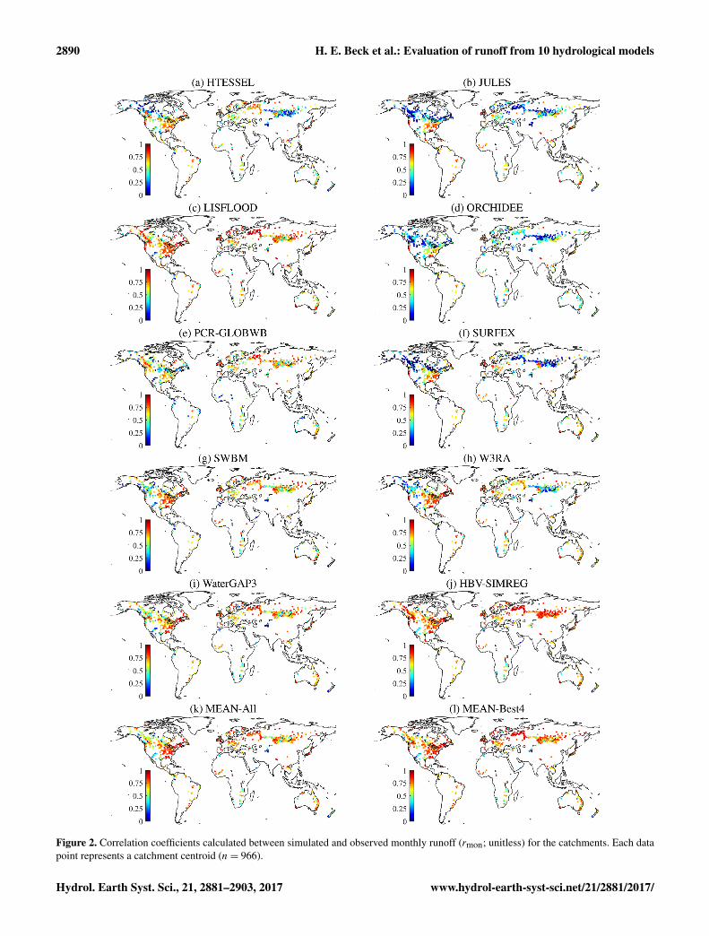
regions. All models showed negative MAR biases in snow-dominated regions such as Alaska, the Rocky Mountains,and southern Russia, while they consistently showed posi-tive MAR biases for the Great Plains (USA) and southernAustralia. Figure 2 shows, for the 10 models and the en-sembles, maps of the correlation between simulated and ob-served monthly flows (rmon) for the catchments, showingthe data underlying the rmon values presented in Table 5.Maps of all other temporal variability metrics are presentedin Figs. S1.9–1.14. In general, the GHMs obtained good rmonvalues for most catchments, while the LSMs obtained moder-ate rmon values for most catchments. All LSMs showed poorto fair rmon values for snow-dominated catchments.

Although the NSE has been widely criticized for beingoverly sensitive to the magnitude and timing of peak flows(e.g., Schaefli and Gupta, 2007; Jain and Sudheer, 2008;Criss and Winston, 2008; Gupta et al., 2009), we did cal-culate NSE scores to allow the present results to be put in thecontext of previous macro-scale studies (see Supplement Ta-ble S1). For most models negative median NSE scores wereobtained, similar to Zhang et al. (2016), who evaluated themonthly and annual runoff estimates from 14 (uncalibrated)macro-scale models in 644 large Australian catchments (>2000 km2). Our scores are, however, slightly lower than thoseobtained by Lohmann et al. (2004) and Xia et al. (2012),who evaluated the daily runoff estimates from four (uncal-ibrated) macro-scale models in about a thousand small-to-medium sized USA catchments (< 10000 km2), but this isprobably attributable to the high quality of the USA forc-ing data (Wu et al., 2017). They are also somewhat lowerthan those obtained by Decharme and Douville (2007), whoevaluated two (uncalibrated) macro-scale models in 80 largecatchments (> 100000 km2) around the globe, but this canbe explained by their much larger catchment sizes.

Figure 3 shows, for the seven models with data on en-ergy availability, density plots of grid cell values of aridityindex (AI; ratio of long-term energy availability to P ) versusRC (ratio of long-term mean runoff to P ), revealing how themodels respond in terms of RC to different climatic condi-tions. Also shown are the energy-limit line for which actualevaporation equals the available energy, the water-limit linefor which runoff equals P , and the Budyko (1974) curve,the most well-known among several similar empirical rela-tionships describing the competition between runoff and ac-tual evaporation (Ol’dekop, 1911; Pike, 1964; Zhang et al.,2001; Porporato et al., 2004). Given its empirical nature, theBudyko curve should only be used for visual reference, andnot to judge the performance of the different models. Be-sides the striking differences in behavior among the mod-els, it can be seen that HTESSEL, JULES, PCR-GLOBWB,W3RA, and WaterGAP3 do not adhere to the water and/orenergy limits (Fig. 3a, b, d, f, and g, respectively). For Wa-terGAP3, this may be due to the use of calibration factors,which have the potential to generate runoff that can go be-yond the physical limits in an effort to compensate for errors



Figure 1. Simulated minus observed square-root-transformed mean annual runoff (MAR; units√

mm yr−1) for the catchments. Each datapoint represents a catchment centroid (n= 966). Red (blue) indicates an overestimated (underestimated) MAR relative to the observations.



Figure 2. Correlation coefficients calculated between simulated and observed monthly runoff (rmon; unitless) for the catchments. Each datapoint represents a catchment centroid (n= 966).



in the P , PET, or streamflow data. For the other models thiscould be indicative of issues with the runoff and/or evapo-ration routines. The larger spread found for the models forwhich we used net radiation to estimate the available energy(HTESSEL, JULES, and SURFEX; Fig. 3a, b, and e, respec-tively) is because the majority of the net radiation is con-verted to sensible heat rather than latent heat in cold climates(Kleidon et al., 2014).

It is generally difficult to gain insight into why a particularmodel performs as it does due to the large number of inter-acting model components, equations, and parameters. Never-theless, the underestimation of runoff by HTESSEL probablyreflects the excessive evaporation by HTESSEL previouslyreported by Haddeland et al. (2011). PCR-GLOBWB mostlikely suffers from suboptimal baseflow-related parametervalues, since its structure is similar to that of LISFLOOD,which performs markedly better. SWBM clearly suffers fromthe absence of a baseflow routine outside (semi-)arid re-gions. Although W3RA and HBV-SIMREG use an identicalsnow routine, W3RA performs considerably worse in snow-dominated regions, probably because HBV-SIMREG usesa snowfall gauge undercatch correction factor. The unsat-isfactory performance demonstrated by the LSMs in snow-dominated regions could be related to deficiencies in thesnow routines or the energy balance estimates (see Sect. 4.3).WaterGAP3 and particularly HBV-SIMREG performed quitewell overall, likely because of their comprehensive calibra-tion (see Sect. 4.4). In any case, the pronounced inter-modelperformance spread found here suggests that model choiceshould be regarded as a critical step in any hydrological mod-eling study. Moreover, it underscores the importance of hy-drological model uncertainty in addition to climate input un-certainty, as also emphasized in several other recent macro-scale studies (Haddeland et al., 2011; Schewe et al., 2013;Prudhomme et al., 2014; Mendoza et al., 2015b; Giuntoliet al., 2015a). Currently, the large majority of studies as-sessing the hydrological impacts of climate change com-pletely neglect hydrological model uncertainty (Teutschbeinand Seibert, 2010).

4.2 How well do the models perform in terms oflong-term runoff trends?

The models displayed very similar MAR trends (Fig. S1.8),meaning they respond similarly to climate variability, giventhat none of the models account for land use or land coverchanges, urbanization, reservoir construction, or increasingatmospheric CO2. However, the models obtained rather lowspatial (Spearman) correlation coefficients (ρMAR trend) rang-ing from 0.32 (SURFEX) to 0.42 (LISFLOOD; Table 5), in-dicating that the simulated MAR trends correspond fairly tomoderately well to the observed ones. These values are lowerthan the (Pearson) correlation coefficients ranging from 0.52to 0.63 obtained by Stahl et al. (2012), who evaluated MARtrends from seven models using observations from 293 small

European catchments (100–1000 km2), presumably due tothe better quality of the European meteorological forcing andobserved streamflow data. Milly et al. (2005) evaluated MARtrends from a 12-model ensemble using observations from165 large catchments (> 50000 km2) around the globe, ob-taining a (Pearson) correlation coefficient of 0.34, which issimilar to ours. These low correlations, which were some-what unexpected given the relative ease with which MAR canbe estimated (e.g., Westerberg and McMillan, 2015; Becket al., 2015), may be indicative of changes in non-climaticdrivers of hydrological change or drift errors in the forcingor observed streamflow data. We expect the inter-model vari-ability in trends to be higher and the agreement with obser-vations to be even lower for seasonal and monthly averagesas well as runoff signatures sensitive to the shape of individ-ual flow events (cf. Bastola et al., 2011; Gosling et al., 2011).Overall, these results suggest that studies using global-scaledatasets to assess the impacts of past climate change onrunoff in small-to-medium-sized catchments should be inter-preted with considerable caution.

4.3 How do the results of the GHMs differ, if at all,from those of the LSMs?

Similar to Haddeland et al. (2011), the LSMs were found toproduce less runoff overall (Table 5 and Fig. 1), perhaps dueto their use of physically based Richards–Darcy type equa-tions, which neglect preferential flows. We further found thatthe GHMs perform, on average, worse than the LSMs in rain-dominated regions: the GHMs (excluding the comprehen-sively calibrated models WaterGAP3 and HBV-SIMREG;see Sect. 4.4) obtained mean OS scores of 0.28, 0.33, and0.43 for tropical, arid, and temperate climates, respectively,while the same values for the LSMs are 0.39, 0.47, and0.47, respectively (Table 5). However, the lower performanceof the GHMs is primarily attributable to PCR-GLOBWBand SWBM. As mentioned before, PCR-GLOBWB probablysuffers from a suboptimal baseflow-related parameterization,while SWBM suffers from the absence of a baseflow routine.

The GHMs do appear to perform consistently better thanthe LSMs in snow-dominated regions: the GHMs (again ex-cluding WaterGAP3 and HBV-SIMREG) obtained mean OSscores of 0.46 and 0.32 for cold and polar climates, respec-tively, while the same values for the LSMs are 0.31 and0.25, respectively (Table 5). The performance of the LSMsappears to be mainly due to a very early bias in flow tim-ing, a very low baseflow contribution, and a misrepresen-tation of the seasonal cycle (Figs. S1.4, S1.5, and S1.13,respectively). Our results are in agreement with Giuntoliet al. (2015b), who found five GHMs to outperform, on aver-age, four LSMs using observations from 252 temperate andcold catchments (64 to 1 350 000 km2) located in the cen-tral USA, and with Zhang et al. (2016), who found that twoLSMs performed considerably worse than two GHMs in coldand polar regions using observations from 644 catchments



Figure 3. Density plots of grid cell values of aridity index (AI) versus runoff coefficient (RC), for the seven models with data on the availableenergy. The green line represents the energy limit for which actual evaporation equals PET, the purple line represents the water limit forwhich runoff equals P , whereas the blue line represents the Budyko (1974) curve.

(> 2000 km2, upper limit not reported) around the globe. Thepoorer performance obtained by the LSMs is probably in-dicative of differences between the snow routines used byGHMs and LSMs. The GHMs use relatively simple concep-tual temperature-index snow routines driven by air tempera-ture, which can be estimated with relative ease, whereas theLSMs use more complex physically based energy balancesnow routines driven by estimates of energy balance compo-nents, which are subject to considerable uncertainty, particu-larly in regions with complex topography (Ferguson, 1999).Although several previous studies have found that the twotypes of snow routines yield comparable performance (e.g.,WMO, 1986; Franz et al., 2008; Zeinivand and De Smedt,2009; Debele et al., 2010), these studies used a very smallnumber of relatively well-instrumented catchments (six, two,one, and three, respectively), which may have led to less-

generalizable conclusions. Overall, it appears that the energybalance estimates and snow routines used by the LSMs re-quire re-evaluation (cf. Zhang et al., 2016).

4.4 Are calibration and regionalization important oreven essential?

Calibration is important for both conceptual and physicallybased hydrological models to provide more accurate runoffestimates, to account for (i) the impossibility of measur-ing all required model parameters at the model applica-tion scale, (ii) lack of process understanding, (iii) possiblyoverly simplistic process representations, (iv) the spatiotem-poral discretization of highly heterogeneous rainfall–runoffprocesses, and (v) errors in the forcing data (Beven, 1989;Blöschl and Sivapalan, 1995; Duan et al., 2001, 2006; Mc-Donnell et al., 2007; Nasonova et al., 2009; Rosero et al.,



2011; Minville et al., 2014). Yet, despite the developmentof numerous calibration techniques over the last 50 years(Dawdy and O’Donnell, 1965; Duan et al., 2004) and thecurrent widespread availability of streamflow observations(Hannah et al., 2011), macro-scale models generally tendto be uncalibrated (Sooda and Smakhtin, 2015; Bierkens,2015; Kauffeldt et al., 2016). This is perhaps mainly dueto (i) the substantial amount of work involved with calibra-tion (e.g., Bock et al., 2015), (ii) the risk of obtaining un-realistic parameters due to equifinality and data issues (An-dréassian et al., 2012), and (iii) the lack of a commonly ac-cepted regionalization technique (Beck et al., 2016). In ad-dition, the modeler may feel that since their model is phys-ically based, it does not require calibration (Beven, 1989).LSMs in particular are rarely calibrated against runoff, likelybecause (i) runoff estimation is generally not among the pri-mary aims of LSMs; (ii) for water transport in the soil, LSMstypically use Richards–Darcy type equations, which are com-putationally expensive and require a fine vertical and tempo-ral soil discretization; and (iii) LSMs often do not accountfor river routing, confounding the calibration of large catch-ments. Instead, the parameters in macro-scale models areusually based on “expert opinion” and thus founded on thebold assumption that the modeler sufficiently understandsthe hydrological processes, feedbacks, and parameter inter-actions taking place within the model for any location onEarth.

Nevertheless, out of the 10 models considered inthis study, four use parameters derived by calibration(LISFLOOD, SWBM, WaterGAP3, and HBV-SIMREGall GHMs). LISFLOOD was calibrated against ob-served streamflow for 24 large catchments (84 230 to4 680 000 km2) across the globe using the WFDEI forcingand an aggregate objective function incorporating bias, NSE,and log-transformed NSE computed from daily streamflowdata. The calibration might have influenced the present eval-uation; although we used much smaller catchments (1000 to5000 km2), 47 % of our catchments are located within thecalibration catchments. SWBM uses a spatially uniform pa-rameter set based on calibration using the E-OBS forcing(Haylock et al., 2008) against European data on such key hy-drologic variables as soil moisture, total water storage, evap-oration, and runoff (Orth and Seneviratne, 2015). For thecalibration against runoff, they used observations from 436small European catchments (mostly < 1000 km2), and con-sidered daily and monthly correlations as well as bias. Thecalibrated parameter set was subsequently applied globally.Besides the addition of a baseflow routine, SWBM wouldprobably benefit from regionalized parameters that vary ac-cording to landscape characteristics. WaterGAP3 has beencalibrated using the WFDEI forcing in terms of bias for theinterstation regions (the catchment of a station excludingthe catchments of nested upstream stations) of 2071 stations(catchment size ranging from 2830 to 966 321 km2) aroundthe globe, some of which have also been used in the current

evaluation. The calibrated parameters were subsequently re-gionalized to ungauged regions using multiple linear regres-sion based on six predictors (Döll et al., 2003). The modeldoes indeed perform very well for MAR and thus RC, butthis did not necessarily translate into good performance forBFI (Table 5, and Figs. 1 and 2). HBV-SIMREG also usesregionalized parameter fields, produced by transferring cali-brated parameters from 674 small-to-medium sized “donor”catchments (10 to 10 000 km2) across the globe to “receptor”grid cells with similar climatic and physiographic character-istics (Beck et al., 2016). In their study, Beck et al. (2016)show that HBV using spatially uniform parameters performswithin the range of the other models, confirming that therelatively good performance of HBV-SIMREG stems fromthe regionalization exercise. In addition, although Beck et al.(2016) did not use the WFDEI forcing for the calibration,they calibrated against several of the performance metricsalso used here and used 179 of our catchments as parameterdonors, further explaining the relatively good performanceobtained by HBV-SIMREG (Table 5, and Figs. 1 and 2).

Overall, it appears that the calibration exercises for Wa-terGAP3, HBV-SIMREG, and possibly LISFLOOD have re-sulted in markedly improved performance. However, Water-GAP3 performed poorly in terms of ρBFI (Table 5), meaningthe calibration of MAR did not translate into better BFI per-formance. These results underscore the benefits of calibratedparameters over a priori parameters (cf. Duan et al., 2006;Hunger and Döll, 2008; Nasonova et al., 2009; Rosero et al.,2011; Greuell et al., 2015; Zhang et al., 2016) and highlightthe importance of using an objective function for the cali-bration that incorporates a broad range of metrics related tovarious important aspects of the hydrograph (cf. Gupta et al.,2008; Vis et al., 2015; Shafii and Tolson, 2015). These resultsalso emphasize the usefulness of regionalization techniques(Parajka et al., 2013), which typically enhance performanceover the entire model domain and are thus of particular valuefor macro-scale modeling, given that the majority of the landsurface is ungauged or poorly gauged (Sivapalan, 2003; Han-nah et al., 2011). However, although there are numerous stud-ies performing regionalization at a regional scale (see re-views by He et al., 2011; Hrachowitz et al., 2013; Razaviand Coulibaly, 2013; Parajka et al., 2013), only a few studieshave attempted regionalization at a macro-scale (see reviewby Beck et al., 2016). We argue that more effort should be de-voted to regionalizing the parameters of macro-scale models(cf. Bierkens, 2015; Döll et al., 2015).

It should be noted, however, that the potential performanceimprovement gained by calibration and regionalization willdepend on the structure and flexibility of the model in ques-tion. Many current models have rigid structures and/or in-sufficient free parameters and thus cannot be calibrated suc-cessfully (Mendoza et al., 2015a). Moreover, for climate pro-jections one should bear in mind that calibrated parametersbecome less valid when the model is subjected to climaticconditions it has never seen before (Knutti, 2008).



4.5 What is the impact of the forcing data on thesimulated runoff?

There are not only strong inter-model differences in the per-formance patterns but also clear inter-model similarities, sug-gesting that the forcing data quality imparts a strong limiton the performance. This is most notable for the MAR met-ric: all models showed negative biases in MAR in snow-dominated regions such as Alaska, the Rocky Mountains, andsouthern Russia, while they consistently showed positive bi-ases in MAR for the Great Plains (USA) and southern Aus-tralia (Fig. 1). The high spatial correlation in the performancepatterns suggests that these consistent performance patternsmay be due to biases in the WFDEI P data, rather than bi-ases in the streamflow observations, which are unlikely to bespatially correlated.

It is conceivable that biases are present in the WFDEI Pdata, because (i) the monthly CRU dataset, which has beenused to correct the WFDEI dataset, is based on only a subsetof the available gauges and does not explicitly account fororographic effects; (ii) in sparsely gauged regions the cor-rection using CRU is more likely to deteriorate rather thanimprove the P estimates; and (iii) the Adam and Lettenmaier(2003) gauge undercatch correction factors are based on in-terpolation of a very sparse sample of gauges and thus sub-ject to considerable uncertainty. For the conterminous USAwe quantified the biases in the WFDEI P data using thehigh-quality Parameter-elevation Relationships on Indepen-dent Slopes Model (PRISM) climatic dataset (Daly et al.,1994), which is based on considerably more gauges thanCRU and includes sophisticated corrections for orography.Figure 4a shows the bias in mean annual P from WFDEIrelative to that from PRISM, suggesting that the WFDEI Pdata are indeed subject to large biases. Figure 4b shows thebias in MAR from the MEAN-All ensemble relative to MARfrom the observations, revealing a comparable bias pattern,thus confirming that the biases in the WFDEI P propagatein the simulated runoff. The correlation coefficient betweenthe MAR and P bias values is 0.58, indicating a moderatelystrong relationship. These P biases appear to translate intoeven more pronounced runoff biases in (semi-)arid regions(notably the northern Great Plains; Fig. 4b and c) due tothe highly nonlinear response behavior in these environments(Lidén and Harlin, 2000; Fekete et al., 2004; Van Dijk et al.,2013a). We were unable to quantify the P biases globallysince no other independent, global-scale P dataset exists (theWorldClim and CHPclim datasets are likely to exhibit simi-lar biases as the CRU TS3.1 dataset, given that they are basedon similar sets of gauges). However, we expect the P biasesto be at least similar, if not more severe, outside the well-instrumented conterminous USA (cf. Fekete et al., 2004; Hi-jmans et al., 2005; Biemans et al., 2009; Zhou et al., 2012;Kauffeldt et al., 2013; Greuell et al., 2015). It should be notedthat biases in PET are probably of secondary importance as

compared with biases in P (Donohue et al., 2010; SpernaWeiland et al., 2011; Seiller and Anctil, 2015).

The global-scale quantification and reduction of these Pbiases should be a priority for future research. Satellite-derived P offers unique opportunities in this regard (e.g.,Funk et al., 2015) that extend beyond the tropics with the re-cent launch of the Global Precipitation Measurement (GPM)mission (Smith et al., 2007). Another little-explored way ofreducing P uncertainty is by “doing hydrology backwards”;that is, to use information on other hydrological variables, forexample, satellite-derived surface soil moisture (e.g., Broccaet al., 2014), streamflow observations (e.g., Adam et al.,2006; Beck et al., 2017), and snow-depth observations (e.g.,Cherry et al., 2005) to reconstruct P through hydrologicalmodeling. Arguably the most important obstacles to combin-ing multiple data sources are the inconsistent temporal cov-erage and scale of different data sources and the general lackof error/uncertainty estimates.

Although the models all used the same P data, they useddifferent formulations to compute PET, which has likely con-tributed to differences in simulated runoff among the modelsin energy-limited regions (Weiß and Menzel, 2008; Kingstonet al., 2009; Haddeland et al., 2011; Weedon et al., 2011;Sperna Weiland et al., 2011). However, PET data were avail-able for only four models, which is insufficient to examinewhether the PET formulation has had a discernible influenceon the simulated runoff, given the numerous other differencesin structure and parameterization among the models.

4.6 How valuable are multi-model ensembles?

The multi-model ensemble MEAN-All incorporated all 10models, while MEAN-Best4 incorporated only LISFLOOD,W3RA, WaterGAP3, and HBV-SIMREG (i.e., the four mod-els that performed best in terms of OS; Table 5). MEAN-Alland MEAN-Best4 were found to perform better than all indi-vidual models (with the exception of HBV-SIMREG, whichhas been comprehensively calibrated; Table 5, and Figs. 1and 2). These results highlight the benefits of multi-modelensembles, in line with several previous studies (Ajami et al.,2006; Duan et al., 2007; Viney et al., 2009; Materia et al.,2010; Velázquez et al., 2010; Gudmundsson et al., 2012a;Xia et al., 2012; Yang et al., 2015). The similar OS scoresobtained by MEAN-All and MEAN-Best4 (0.57 and 0.60,respectively; Table 5) suggests that the inclusion of less-accurate models has only limited adverse effects. It may beworthwhile for future studies to examine the benefits of moresophisticated multi-model combination techniques involvingbias correction or model weighting (e.g., Ajami et al., 2006;Duan et al., 2007; Bohn et al., 2010). These weights can sub-sequently be transferred from gauged to ungauged areas us-ing regionalization techniques typically used for hydrologi-cal model parameters (Blöschl et al., 2013).

HBV-SIMREG differs from the other models becauseit represents a “multi-parameterization ensemble”, which



Figure 4. For the conterminous USA, (a) the bias in mean annual P from WFDEI relative to PRISM, (b) the bias in MAR from the MEAN-All ensemble relative to the observations, and (c) the aridity index, the ratio of mean annual PET (computed from PRISM air temperatureusing Hargreaves et al., 1985) to P (PRISM; note the nonlinear color scale). Each data point in (b) represents a catchment centroid. Thebias in (a) and (b) was computed following B = (X−R)/(X+R), where B is the bias, X the uncertain value, and R the reference value.B values range from −1 to 1. A 100 % overestimation results in B = 1/3, whereas a 50 % underestimation results in B =−1/3.

means the model was run multiple (10) times globally usingdifferent (regionalized) parameter sets representing differ-ent catchment response behaviors (Beck et al., 2016). HBV-SIMREG obtained slightly better performance than bothMEAN-All and MEAN-Best4 overall (Table 5), tentativelysuggesting that a multi-parameterization ensemble for a sin-gle, sufficiently flexible model provides performance com-parable to a multi-model ensemble (cf. Oudin et al., 2006;Yang et al., 2011; Coxon et al., 2014). If this is confirmed,it would negate the need to set up, run, and maintain mul-tiple models, and incentivize the development of a singlecommunity hydrological model (cf. Weiler and Beven, 2015)as well as modeling systems allowing for the selection ofalternative model structures (cf. Bierkens, 2015), such asthe Framework for Understanding Structural Errors (FUSE;Clark et al., 2008), Noah Multi-Parameterization (Noah-MP;Niu et al., 2011), and SUPERFLEX (Fenicia et al., 2011).

4.7 Do all models show the early bias in runoff timingin snow-dominated catchments previouslydocumented and what is the cause?

With the exception of ORCHIDEE and HBV-SIMREG, allmodels showed early T50 biases in snow-dominated regions(Fig. S1.3), indicating that the models produce the springsnowmelt peak early, as has also been reported in severalprevious studies using different models and forcing data(Lohmann et al., 2004; Slater et al., 2007; Decharme andDouville, 2007; Balsamo et al., 2009; Zaitchik et al., 2010;Beck et al., 2015). The early runoff timing is probably pri-

Figure 5. Scatterplot of the difference between simulated (MEAN-All) and observed-transformed RC (DRC) versus the difference be-tween simulated (MEAN-All) and observed T50 (DT50) for thecatchments (n= 966).

marily due to P underestimation, which leads to insuffi-cient snow accumulation that subsequently melts too quickly(Hancock et al., 2014). The fact that HBV-SIMREG per-forms well in this regard is probably attributable to the snow-fall gauge undercatch correction factor of the model. Indeed,Fig. 5 tentatively shows that catchments in which the modelsstrongly underestimate runoff (i.e., negative DRC) generally



tend to exhibit an early bias in T50 (i.e., negative DT50) andvice versa. The absence or misrepresentation of certain pro-cesses that delay snowmelt runoff in the models may haveexacerbated the early runoff timing problem. Examples ofsuch processes include the isothermal phase change of thesnowpack, retainment of meltwater in the snowpack in porespaces, infiltration of meltwater into the soil, meltwater re-freezing during cold days and nights, and ice jams in rivers.On the whole, more research is needed to ascertain the exactreasons of the early runoff timing.

5 Conclusions

The runoff estimates from 10 state-of-the-art macro-scalehydrological models, all forced with the WFDEI dataset,were evaluated using observations from 966 medium-sizedcatchments around the globe. With reference to the questionsposed in the introduction, the following was found:

1. The performance differed markedly among models, un-derscoring the importance of hydrological model uncer-tainty in addition to climate input uncertainty, and sug-gesting that model choice should be regarded as a criti-cal step in any hydrological modeling study.

2. The models displayed similar MAR trends, althoughthey were in poor agreement with observed trends.Model-based runoff trends in small-to-medium sizedcatchments should thus be interpreted with considerablecaution.

3. Considering only the uncalibrated models, the GHMsperformed similarly to the LSMs in rainfall-dominatedregions but consistently better than the LSMs in snow-dominated regions, perhaps due to the use of more data-demanding snow routines or the misrepresentation offrozen soil and snowmelt processes by the LSMs.

4. The models that have been calibrated obtained higherscores for the performance metrics incorporated in therespective objective functions used for calibration.

5. The WFDEI P forcing data still appear to contain sub-stantial biases, despite adjustments using gauge obser-vations. These P biases translate into biases in the simu-lated runoff, which are amplified in (semi-)arid regions.In snow-dominated regions there appears to be a consis-tent underestimation in P and thus simulated runoff.

6. The multi-model ensembles obtained only slightlyworse performance than the best (calibrated) model, andthe inclusion of less-accurate models did not severelydegrade the performance. A multi-parameterization en-semble for a single, sufficiently flexible model is easierto realize but we speculate may yield the same perfor-mance benefits as a multi-model ensemble.

7. Most models were indeed found to generate the springsnowmelt peak early, probably due to the previouslymentioned P underestimation and the absence or mis-representation of certain processes that delay snowmeltrunoff in the models.

Data availability. All model outputs are available viathe eartH2Observe Water Cycle Integrator (WCI; http://wci.earth2observe.eu).

The Supplement related to this article is availableonline at https://doi.org/10.5194/hess-21-2881-2017-supplement.

Author contributions. H. B. designed and performed the modelevaluation and wrote most of the manuscript. A. v. D., A. d. R.,E. D., G. F., R. O., and J. S. helped with the interpretation of theresults and contributed to writing of the manuscript. H. B., A. v. D.,A. d. R., E. D., G. F., and R. O. assisted in running the hydrologicalmodels and making available the model output.

Competing interests. The authors declare that they have no conflictof interest.

Acknowledgements. The Global Runoff Data Centre (GRDC) andthe US Geological Survey (USGS) are thanked for providing mostof the observed streamflow data. We gratefully acknowledge themodeling groups participating in the eartH2Observe project forproviding the simulated runoff data. Lukas Gudmundsson and ananonymous reviewer are thanked for their comments on an earlierdraft. This research received funding from the European UnionSeventh Framework Programme (FP7/2007–2013) under grantagreement no. 603608, “Global Earth Observation for integratedwater resource assessment”: eartH2Observe. The views expressedherein are those of the authors and do not necessarily reflect thoseof the European Commission.

Edited by: S. SchymanskiReviewed by: L. Gudmundsson and one anonymous referee

References

Adam, J. C. and Lettenmaier, D. P.: Adjustment of global griddedprecipitation for systematic bias, J. Geophys. Res.-Atmos., 108,4257, https://doi.org/10.1029/2002JD002499, 2003.

Adam, J. C., Clark, E. A., Lettenmaier, D. P., and Wood, E. F.: Cor-rection of global precipitation products for orographic effects, J.Clim., 19, 15–38, https://doi.org/10.1175/JCLI3604.1, 2006.

Ajami, N. K., Duan, Q., Gao, X., and Sorooshian, S.: MultimodelCombination Techniques for Analysis of Hydrological Simula-tions: Application to Distributed Model Intercomparison ProjectResults, J. Hydrometeorol., 7, 755–768, 2006.




https://doi.org/10.5194/hess-21-2881-2017-supplement

https://doi.org/10.5194/hess-21-2881-2017-supplement

https://doi.org/10.1029/2002JD002499

https://doi.org/10.1175/JCLI3604.1


Andréassian, V., Lerat, J., Loumagne, C., Mathevet, T., Michel, C.,Oudin, L., and Perrin, C.: What is really undermining hydrologicscience today?, Hydrol. Process., 21, 2819–2822, 2007.

Andréassian, V., Le Moine, N., Perrin, C., Ramos, M. H., Oudin,L., Mathevet, T., Lerat, J., and Berthet, L.: All that glitters isnot gold: the case of calibrating hydrological models, Hydrol.Process., 26, 2206–2210, 2012.

Balsamo, G., Beljaars, A., Scipal, K., Viterbo, P., van den Hurk,B., Hirschi, M., and Betts, A. K.: A revised hydrology for theECMWF model: verification from field site to terrestrial waterstorage and impact in the integrated forecast system, J. Hydrom-eteorol., 10, 623–643, 2009.

Balsamo, G., Pappenberger, F., Dutra, E., Viterbo, P., and van denHurk, B.: A revised land hydrology in the ECMWF model: a steptowards daily water flux prediction in a fully-closed water cycle,Hydrol. Process., 25, 1046–1054, 2011.

Bastola, S., Murphy, C., and Sweeney, J.: The role of hydrologicalmodeling uncertainties in climate change impact assessments ofIrish river catchments, Adv. Water Resour., 34, 562–576, 2011.

Beck, H. E., van Dijk, A. I. J. M., Miralles, D. G., de Jeu, R. A. M.,Bruijnzeel, L. A., McVicar, T. R., and Schellekens, J.: Globalpatterns in baseflow index and recession based on streamflow ob-servations from 3394 catchments, Water Resour. Res., 49, 7843–7863, 2013.

Beck, H. E., van Dijk, A. I. J. M., and de Roo, A.: Global mapsof streamflow characteristics based on observations from severalthousand catchments, J. Hydrometeorol., 16, 1478–1501, 2015.

Beck, H. E., van Dijk, A. I. J. M., de Roo, A., Mi-ralles, D. G., McVicar, T. R., Schellekens, J., and Brui-jnzeel, L. A.: Global-scale regionalization of hydrologicmodel parameters, Water Resour. Res., 52, 3599–3622,https://doi.org/10.1002/2015WR018247, 2016.

Beck, H. E., van Dijk, A. I. J. M., Levizzani, V., Schellekens,J., Miralles, D. G., Martens, B., and de Roo, A.: MSWEP: 3-hourly 0.25◦ global gridded precipitation (1979–2015) by merg-ing gauge, satellite, and reanalysis data, Hydrol. Earth Syst. Sci.,21, 589–615, https://doi.org/10.5194/hess-21-589-2017, 2017.

Best, M. J., Pryor, M., Clark, D. B., Rooney, G. G., Essery, R. .L. H., Ménard, C. B., Edwards, J. M., Hendry, M. A., Porson, A.,Gedney, N., Mercado, L. M., Sitch, S., Blyth, E., Boucher, O.,Cox, P. M., Grimmond, C. S. B., and Harding, R. J.: The JointUK Land Environment Simulator (JULES), model description— Part 1: Energy and water fluxes, Geosci. Model Dev., 4, 677–699, https://doi.org/10.5194/gmd-4-677-2011, 2011.

Beven, K. J.: Changing ideas in hydrology — the case of physically-based models, J. Hydrol., 105, 157–172, 1989.

Biemans, H., Hutjes, R. W. A., Kabat, P., Strengers, B. J., Gerten,D., and Rost, S.: Effects of precipitation uncertainty on dischargecalculations for main river basins, J. Hydrometeorol., 10, 1011–1025, 2009.

Bierkens, M. F. P.: Global hydrology 2015: state, trends,and directions, Water Resour. Res., 51, 4923–4947,https://doi.org/10.1002/2015WR017173, 2015.

Bierkens, M. F. P., Bell, V. A., Burek, P., Chaney, N., Condon, L. E.,David, C. H., de Roo, A., Döll, P., Drost, N., Famiglietti, J. S.,Flörke, M., Gochis, D. J., Houser, P., Hut, R., Keune, J., Kol-let, S., Maxwell, R. M., Reager, J. T., Samaniego, L., Sudicky,E., Sutanudjaja, E. H., van de Giesen, N., Winsemius, H., and

Wood, E.: Hyper-resolution global hydrological modelling: whatis next?, Hydrol. Process., 29, 310–320, 2015.

Blöschl, G. and Sivapalan, M.: Scale issues in hydrological mod-elling: A review, Hydrol. Process., 9, 251–290, 1995.

Blöschl, G., Sivapalan, M., Wagener, T., Viglione, A., and Savenije,H., eds.: Runoff Prediction in Ungauged Basins: synthesis acrossProcesses, Places and Scales, Cambridge University Press, NewYork, US, 2013.

Bock, A. R., Hay, L. E., McCabe, G. J., Markstrom, S. L., andAtkinson, R. D.: Parameter regionalization of a monthly waterbalance model for the conterminous United States, Hydrol. EarthSyst. Sci., 20, 2861–2876, https://doi.org/10.5194/hess-20-2861-2016, 2016.

Bohn, T. J., Sonessa, M. Y., and Lettenmaier, D. P.: Seasonal hydro-logic forecasting: do multimodel ensemble averages always yieldimprovements in forecast skill?, J. Hydrometeorol., 11, 1358–1372, 2010.

Bontemps, S., Defourny, P., and van Bogaert, E.: GlobCover 2009,products description and validation report, Tech. rep., ESA Glob-Cover project, available at: http://ionia1.esrin.esa.int (last access:June 2016), 2011.

Bosch, J. M. and Hewlett, J. D.: A review of catchment experimentsto determine the effect of vegetation changes on water yield andevapotranspiration, J. Hydrol., 55, 3–23, 1982.

Breuer, L., Huisman, J. A., Willems, P., Bormann, H., Bronstert, A.,Croke, B. F. W., Frede, H., Gräffe, T., Hubrechts, L., Jakeman,A. J., Kite, G., Lanini, J., Leavesley, G., Lettenmaier, D. P., Lind-ström, G., Seibert, J., Sivapalan, M., and Viney, N. R.: Assessingthe impact of land use change on hydrology by ensemble model-ing (LUCHEM). I: Model intercomparison with current land use,Adv. Water Resour., 32, 129–146, 2009.

Brocca, L., Ciabatta, L., Massari, C., Moramarco, T., Hahn, S.,Hasenauer, S., Kidd, R., Dorigo, W., Wagner, W., and Levizzani,V.: Soil as a natural rain gauge: estimating global rainfall fromsatellite soil moisture data, J. Geophys. Res.-Atmos., 119, 5128–5141, 2014.

Budyko, M. I.: Climate and life, Academic Press, New York, 1974.Burek, P., van der Knijff, J., and de Roo, A.: LISFLOOD Distributed

Water Balance and Flood Simulation Model Revised User Man-ual, Tech. Rep. EUR 26162 EN, Joint Research Centre (JRC),Ispra, Italy, https://doi.org/10.2788/24719, 2013.

Cherry, J. E., Tremblay, L. B., Déry, S. J., and Stieglitz, M.: Re-constructing solid precipitation from snow depth measurementsand a land surface model, Water Resour. Res., 41, W09401,https://doi.org/10.1029/2005WR003965, 2005.

Clark, M. P., Slater, A. G., Rupp, D. E., Woods, R. A., Vrugt, J. A.,Gupta, H. V., Wagener, T., and Hay, L. E.: Framework for Under-standing Structural Errors (FUSE): a modular framework to di-agnose differences between hydrological models, Water Resour.Res., 44, W00B02, https://doi.org/10.1029/2007WR006735,2008.

Clark, M. P., Fan, Y., Lawrence, D. M., Adam, J. C., Bolster,D., Gochis, D. J., Hooper, R. P., Kumar, M., Leung, L. R.,Mackay, D. S., Maxwell, R. M., Shen, C., Swenson, S. C., andZeng, X.: Improving the representation of hydrologic processesin Earth System Models, Water Resour. Res., 51, 5929–5956,https://doi.org/10.1002/2015WR017096, 2015.

Coxon, G., Freer, J., Wagener, T., Odoni, N. A., and Clark, M.: Di-agnostic evaluation of multiple hypotheses of hydrological be-


https://doi.org/10.1002/2015WR018247

https://doi.org/10.5194/hess-21-589-2017

https://doi.org/10.5194/gmd-4-677-2011

https://doi.org/10.1002/2015WR017173



http://ionia1.esrin.esa.int

https://doi.org/10.2788/24719

https://doi.org/10.1029/2005WR003965

https://doi.org/10.1029/2007WR006735

https://doi.org/10.1002/2015WR017096


havior in a limits-of-acceptability framework for 24 UK catch-ments, Hydrol. Process., 28, 6135–6150, 2014.

Criss, R. E. and Winston, W. E.: Do Nash values have value?Discussion and alternate proposals, Hydrol. Process., 22, 2723–2725, 2008.

Daly, C., Neilson, R. P., and Phillips, D. L.: A statistical-topographic model for mapping climatological precipitation overmountainous terrain, J. Appl. Meteorol., 33, 140–158, 1994.

Dawdy, D. R. and O’Donnell, T.: Mathematical models of catch-ment behavior, J. Hydr. Eng. Div.-ASCE, 91, 123–137, 1965.

Debele, B., Srinivasan, R., and Gosain, A. K.: Comparison ofProcess-Based and Temperature-Index Snowmelt Modeling inSWAT, Water Resour. Manag., 24, 1065–1088, 2010.

Decharme, B.: Influence of runoff parameterization on conti-nental hydrology: Comparison between the Noah and theISBA land surface models, J. Geophys. Res., 112, D19108,https://doi.org/10.1029/2007JD008463, 2007.

Decharme, B. and Douville, H.: Uncertainties in the GSWP-2 pre-cipitation forcing and their impacts on regional and global hy-drological simulations, Clim. Dynam., 27, 695–713, 2006.

Decharme, B. and Douville, H.: Global validation of the ISBA sub-grid hydrology, Clim. Dynam., 29, 21–37, 2007.

Decharme, B., Boone, A., Delire, C., and Noilhan, J.: Lo-cal evaluation of the Interaction between Soil Biosphere At-mosphere soil multilayer diffusion scheme using four pedo-transfer functions, J. Geophys. Res.-Atmos., 116, D20126,https://doi.org/10.1029/2011JD016002, 2011.

Decharme, B., Martin, E., and Faroux, S.: Reconciling soil ther-mal and hydrological lower boundary conditions in land surfacemodels, J. Geophys. Res.-Atmos., 118, 7819–7834, 2013.

Dirmeyer, P. A.: A history and review of the Global Soil WetnessProject (GSWP), J. Hydrometeorol., 12, 729–749, 2011.

Döll, P. and Fiedler, K.: Global-scale modeling of ground-water recharge, Hydrol. Earth Syst. Sci., 12, 863–885,https://doi.org/10.5194/hess-12-863-2008, 2008.

Döll, P., Kaspar, F., and Lehner, B.: A global hydrological modelfor deriving water availability indicators: model tuning and vali-dation, J. Hydrol., 270, 105–134, 2003.

Döll, P., Douville, H., Güntner, A., Müller Schmied, H., andWada, Y.: Modelling Freshwater Resources at the globalscale: challenges and prospects, Surv. Geophys., 37, 1–26,https://doi.org/10.1007/s10712-015-9343-1, 2015.

Donohue, R. J., McVicar, T. R., and Roderick, M. L.: Assessingthe ability of potential evaporation formulations to capture thedynamics in evaporative demand within a changing climate, J.Hydrol., 386, 186–197, 2010.

Duan, Q., Schaake, J., and Koren, V.: A Priori estimation of landsurface model parameters, in: Land Surface Hydrology, Meteo-rology, and Climate: Observations and Modeling, edited by: Lak-shmi, V., Albertson, J., and Schaake, J., no. 3 in Water Scienceand Application, AGU, Washington, DC, US, 77–94, 2001.

Duan, Q., Gupta, H. V., Sorooshian, S., Rousseau, A. N., and Tur-cotte, R.: Calibration of watershed models, vol. Water Scienceand Application, American Geophysical Union, 2004.

Duan, Q., Schaake, J., Andréassian, V., Franks, S., Goteti, G.,Gupta, H. V., Gusev, Y. M., Habets, F., Hall, A., Hay, L., Hogue,T., Huang, M., Leavesley, G., Liang, X., Nasonova, O. N., Noil-han, J., Oudin, L., Sorooshian, S., Wagener, T., and Wood,E. F.: Model Parameter Estimation Experiment (MOPEX): An

overview of science strategy and major results from the secondand third workshops, J. Hydrol., 320, 3–17, 2006.

Duan, Q., Ajami, N. K., Gao, X., and Sorooshian, S.: Multi-modelensemble hydrologic prediction using Bayesian model averag-ing, Adv. Water Resour., 30, 1371–1386, 2007.

Falcone, J. A., Carlisle, D. M., Wolock, D. M., and Meador, M. R.:GAGES: A stream gage database for evaluating natural and al-tered flow conditions in the conterminous United States, Ecol-ogy, 91, 621, 2010.

Fekete, B. M., Vörösmarty, C. J., Roads, J. O., and Willmott, C. J.:Uncertainties in precipitation and their impacts on runoff esti-mates, J. Clim., 17, 294–304, 2004.

Fekete, B. M., Looser, U., Pietroniro, A., and Robarts, R. D.: Ratio-nale for monitoring discharge on the ground, J. Hydrometeorol.,13, 1977–1986, 2012.

Fenicia, G., Kavetski, D., and Savenije, H. H. G.: Elements of aflexible approach for conceptual hydrological modeling: 1. Mo-tivation and theoretical development, Water Resour. Res., 47,https://doi.org/10.1029/2010WR010174, 2011.

Ferguson, R. I.: Snowmelt runoff models, Prog. Phys. Geog., 23,205–227, 1999.

Franz, K. J., Hogue, T. S., and Sorooshian, S.: Operational snowmodeling: Addressing the challenges of an energy balance modelfor National Weather Service forecasts, J. Hydrol., 360, 48–66,2008.

Freeze, R. A. and Harlan, R. L.: Blueprint for a physically-based,digitally-simulated hydrologic response model, J. Hydrol., 9,237–258, 1969.

Funk, C., Verdin, A., Michaelsen, J., Peterson, P., Pedreros, D., andHusak, G.: A global satellite assisted precipitation climatology,Earth Syst. Sci. Data, 7, 275–287, https://doi.org/10.5194/essd-7-275-2015, 2015.

Giuntoli, I., Vidal, J., Prudhomme, C., and Hannah, D. M.: Futurehydrological extremes: the uncertainty from multiple global cli-mate and global hydrological models, Earth Syst. Dynam., 6,267–285, 2015a.

Giuntoli, I., Vilarini, G., Prudhomme, C., Mallakpour, I., and Han-nah, D. M.: Evaluation of global impact models’ ability to re-produce runoff characteristics over the central United States, J.Geophys. Rese.-Atmos., 120, 9138–9159, 2015b.

Gosling, S. N., Taylor, R. G., Arnell, N. W., and Todd,M. C.: A comparative analysis of projected impacts of cli-mate change on river runoff from global and catchment-scalehydrological models, Hydrol. Earth Syst. Sci., 15, 279–294,https://doi.org/10.5194/hess-15-279-2011, 2011.

Greuell, W., Andersson, J. C. M., Donnelly, C., Feyen, L., Gerten,D., Ludwig, F., Pisacane, G., Roudier, P., and Schaphoff,S.: Evaluation of five hydrological models across Europeand their suitability for making projections under climatechange, Hydrol. Earth Syst. Sci. Discuss., 12, 10289–10330,https://doi.org/10.5194/hessd-12-10289-2015, 2015.

Gudmundsson, L. and Seneviratne, S. I.: Towards observation-based gridded runoff estimates for Europe, Hydrol. Earth Syst.Sci., 19, 2859–2879, https://doi.org/10.5194/hess-19-2859-2015,2015.

Gudmundsson, L., Tallaksen, L. M., Stahl, K., Clark, D. B., Du-mont, E., Hagemann, S., Bertrand, N., Gerten, D., Heinke, J.,Hanasaki, N., Voss, F., and Koirala, S.: Comparing Large-Scale


https://doi.org/10.1029/2007JD008463

https://doi.org/10.1029/2011JD016002


https://doi.org/10.1007/s10712-015-9343-1

https://doi.org/10.1029/2010WR010174

https://doi.org/10.5194/essd-7-275-2015

https://doi.org/10.5194/essd-7-275-2015


https://doi.org/10.5194/hessd-12-10289-2015



Hydrological Model Simulations to Observed Runoff Percentilesin Europe, J. Hydrometeorol., 13, 604–620, 2012a.

Gudmundsson, L., Wagener, T., Tallaksen, L. M., and Engeland, K.:Evaluation of nine large-scale hydrological models with respectto the seasonal runoff climatology in Europe, Water Resour. Res.,48, W11504, https://doi.org/10.1029/2011WR010911, 2012b.

Güntner, A.: Improvement of global hydrological models usingGRACE data, Surv. Geophys., 29, 375–397, 2008.

Guo, Z., Dirmeyer, P. A., Gao, X., and Zhao, M.: Improving thequality of simulated soil moisture with a multi-model ensembleapproach, Q. J. R. Meteor. Soc., 133, 731–747, 2007.

Gupta, H. V., Wagener, T., and Liu, Y.: Reconciling theory withobservations: elements of a diagnostic approach to model evalu-ation, Hydrol. Process., 22, 3802–3813, 2008.

Gupta, H. V., Kling, H., Yilmaz, K. K., and Martinez, G. F.: Decom-position of the mean squared error and NSE performance criteria:Implications for improving hydrological modelling, J. Hydrol.,370, 80–91, 2009.

Gupta, H. V., Perrin, C., Blöschl, G., Montanari, A., Kumar, R.,Clark, M., and Andréassian, V.: Large-sample hydrology: a needto balance depth with breadth, Hydrol. Earth Syst. Sci., 18, 463–477, https://doi.org/10.5194/hess-18-463-2014, 2014.

Gustard, A., Bullock, A., and Dixon, J. M.: Low flow estimationin the United Kingdom, Tech. Rep. 108, Institute of Hydrology,Wallingford, UK, 1992.

Haddeland, I., Clark, D. B., Franssen, W., F, L., Voß, F., Arnell,N. W., Bertrand, N., Best, M., Folwell, S., Gerten, D., Gomes,S., Gosling, S. N., Hagemann, S., Hanasaki, N., Harding, R.,Heinke, J., Kabat, P., Koirala, S., Oki, T., Polcher, J., Stacke, T.,Viterbo, P., Weedon, G. P., and Yehm, P.: Multimodel Estimateof the Global Terrestrial Water Balance: Setup and First Results,J. Hydrometeorol., 12, 869–884, 2011.

Hancock, S., Huntley, B., Ellis, R., and Baxter, R.: Biases in Re-analysis Snowfall Found by Comparing the JULES Land SurfaceModel to GlobSnow, J.Clim., 27, 624–632, 2014.

Hannah, D. M., Demuth, S., Van Lanen, H. A. J., Looser, U., Prud-homme, C., Rees, G., Stahl, K., and Tallaksen, L. M.: Large-scaleriver flow archives: importance, current status and future needs,Hydrol. Process., 25, 1191–1200, 2011.

Hansen, M. C., Potapov, P. V., Moore, R., Hancher, M., Turubanova,S. A., Tyukavina, A., Thau, D., Stehman, S. V., Goetz, S. J.,Loveland, T. R., Kommareddy, A., Egorov, A., Chini, L., Justice,C. O., and Townshend, J. R. G.: High-resolution global maps of21st-century forest cover change, Science, 342, 850–853, 2013.

Hargreaves, G. L., Hargreaves, G. H., and Riley, J. P.: Irrigationwater requirements for Senegal River Basin, J. Irrig. Drain. E.-ASCE, 111, 265–275, 1985.

Harris, I., Jones, P. D., Osborn, T. J., and Lister, D. H.: Updatedhigh-resolution grids of monthly climatic observations – theCRU TS3.10 dataset, Int. J. Climatol., 34, 623–642, 2013.

Haylock, M. R., Hofstra, N., Klein Tank, A. M. G., Klok,E. J., Jones, P., and New, M.: A European daily high-resolution gridded data set of surface temperature and precipi-tation for 1950–2006, J. Geophys. Res.-Atmos., 113, D20119,https://doi.org/10.1029/2008JD010201, 2008.

He, Y., Bárdossy, A., and Zehe, E.: A review of regionalisation forcontinuous streamflow simulation, Hydrol. Earth Syst. Sci., 15,3539–3553, https://doi.org/10.5194/hess-15-3539-2011, 2011.

Hijmans, R. J., Cameron, S. E., Parra, J. L., Jones, P. G., and Jarvis,A.: Very high resolution interpolated climate surfaces for globalland areas, Int. J. Climatol., 25, 1965–1978, 2005.

Hrachowitz, M., Savenije, H. H. G., Blöschl, G., McDonnell, J. J.,Sivapalan, M., Pomeroy, J. W., Arheimer, B., Blume, T., Clark,M. P., Ehret, U., Fenicia, F., Freer, J. E., Gelfan, A., Gupta, H. V.,Hughes, D. A., Hut, R. W., Montanari, A., Pande, S., Tetzlaff,D., Troch, P. A., Uhlenbrook, S., Wagener, T., Winsemius, H. C.,Woods, R. A., Zehe, E., and Cudennec, C.: A decade of Predic-tions in Ungauged Basins (PUB) – a review, Hydrol. Sci. J., 58,1198–1255, 2013.

Hunger, M. and Döll, P.: Value of river discharge data for global-scale hydrological modeling, Hydrol. Earth Syst. Sci., 12, 841–861, https://doi.org/10.5194/hess-12-841-2008, 2008.

Jain, S. K. and Sudheer, K. P.: Fitting of hydrologic models: a closelook at the Nash-Sutcliffe index, J. Hydrol. Engin., 13, 981–986,2008.

Jiménez, C., Prigent, C., Mueller, B., Seneviratne, S. I., Mc-Cabe, M. F., Wood, E. F., Rossow, W. B., Balsamo, G., Betts,A. K., Dirmeyer, P. A., Fisher, J. B., Jung, M., Kanamitsu,M., Reichle, R. H., Reichstein, M., Rodell, M., Sheffield, J.,Tu, K., and Wang, K.: Global intercomparison of 12 landsurface heat flux estimates, J. Geophys. Res., 116, D02102,https://doi.org/10.1029/2010JD014545, 2011.

Kauffeldt, A., Halldin, S., Rodhe, A., Xu, C.-Y., and West-erberg, I. K.: Disinformative data in large-scale hydrolog-ical modelling, Hydrol. Earth Syst. Sci., 17, 2845–2857,https://doi.org/10.5194/hess-17-2845-2013, 2013.

Kauffeldt, A., Wetterhall, F., Pappenberger, F., Salamon, P.,and Thielen, J.: Technical review of large-scale hydrologi-cal models for implementation in operational flood forecastingschemes on continental level, Environ. Modell. Soft., 75, 68–76,https://doi.org/10.1016/j.envsoft.2015.09.009, 2016.

Kingston, D. G., Todd, M. C., Taylor, R. G., Thompson, J. R., andArnell, N. W.: Uncertainty in the estimation of potential evap-otranspiration under climate change, Geophys. Res. Lett., 36,L20403, https://doi.org/10.1029/2009GL040267, 2009.

Kleidon, A., Renner, M., and Porada, P.: Estimates of the climato-logical land surface energy and water balance derived from maxi-mum convective power, Hydrol. Earth Syst. Sci., 18, 2201–2218,https://doi.org/10.5194/hess-18-2201-2014, 2014.

Klemeš, V.: Operational testing of hydrological simulation models,Hydrol. Sci. J., 31, 13–24, 1986.

Knutti, R.: Should we believe model predictions of future climatechange?, Philos. T. R. Soc. Lond. S-A, 366, 4647–4664, 2008.

Krinner, G., Viovy, N., de Noblet-Ducoudré, N., Ogée, J., Polcher,J., Friedlingstein, P., Ciais, P., Sitch, S., and Prentice, I. C.:A dynamic global vegetation model for studies of the cou-pled atmosphere-biosphere system, Global Biogeochem. Cy., 19,GB1015, https://doi.org/10.1029/2003GB002199, 2005.

Lehner, B.: Derivation of watershed boundaries for GRDC gaug-ing stations based on the HydroSHEDS drainage network, Tech.Rep. 41, Global Runoff Data Centre (GRDC), Federal Instituteof Hydrology (BfG), Koblenz, Germany, 2012.

Lehner, B., Reidy Liermann, C., Revenga, C., Vörösmarty, C.,Fekete, B., Crouzet, P., Döll, P., Endejan, M., Frenken, K.,Magome, J., Nilsson, C., Robertson, J. C., Rödel, R., Sindorf, N.,and Wisser, D.: High resolution mapping of the world’s reser-


https://doi.org/10.1029/2011WR010911


https://doi.org/10.1029/2008JD010201



https://doi.org/10.1029/2010JD014545


https://doi.org/10.1016/j.envsoft.2015.09.009

https://doi.org/10.1029/2009GL040267


https://doi.org/10.1029/2003GB002199


voirs and dams for sustainable river flow management, Front.Ecol. Environ., 9, 494–502, 2011.

Lidén, R. and Harlin, J.: Analysis of conceptual rainfall-runoff mod-elling performance in different climates, J. Hydrol., 238, 231–247, 2000.

Linsley, R. K. and Crawford, N. H.: Computation of a syntheticstreamflow record on a digital computer, International Associa-tion of Scientific Hydrology, 526–538, 1960.

Lohmann, D., Mitchell, K. E., Houser, P. R., Wood, E. F., Schaake,J. C., Robock, A., Cosgrove, B. A., Sheffield, J., Duan, Q.,Luo, L., Higgins, R. W., Pinker, R. T., and Tarpley, J. D.:Streamflow and water balance intercomparisons of four landsurface models in the North American Land Data Assimila-tion System project, J. Geophys. Res.-Atmos., 109, D07S91,https://doi.org/10.1029/2003JD003517, 2004.

Materia, S., Dirmeyer, P. A., Guo, Z., Alessandri, A., and Navarra,A.: The Sensitivity of Simulated River Discharge to Land SurfaceRepresentation and Meteorological Forcings, J. Hydrometeorol.,11, 334–351, 2010.

McCabe, M. F., Ershadi, A., Jimenez, C., Miralles, D. G., Michel,D., and Wood, E. F.: The GEWEX LandFlux project: eval-uation of model evaporation using tower-based and globally-gridded forcing data, Geosci. Model Dev., 9, 283–305,https://doi.org/10.5194/gmd-9-283-2016, 2016.

McDonnell, J. J., Sivapalan, M., Vaché, K., Dunn, S., Grant,G., Haggerty, R., Hinz, C., Hooper, R., Kirchner, J., Rod-erick, M. L., Selker, J., and Weiler, M.: Moving be-yond heterogeneity and process complexity: a new visionfor watershed hydrology, Water Resour. Res., 43, W07301,https://doi.org/10.1029/2006WR005467, 2007.

Mendoza, P. A., Clark, M. P., Barlage, M., Rajagopalan,B., Samaniego, L., Abramowitz, G., and Gupta, H.: Arewe unnecessarily constraining the agility of complexprocess-based models?, Water Resour. Res., 51, 716–728,https://doi.org/10.1002/2014WR015820, 2015a.

Mendoza, P. A., Clark, M. P., Mizukami, N., Newman, A. J., Bar-lage, M., Gutmann, E. D., Rasmussen, R. M., Rajagopalan, B.,Brekke, L. D., and Arnold, J. R.: Effects of hydrologic modelchoice and calibration on the portrayal of climate change im-pacts, J. Hydrometeorol., 16, 762–780, 2015b.

Milly, P. C. D., Dunne, K. A., and Vecchia, A. V.: Global pattern oftrends in streamflow and water availability in a changing climate,Nature, 438, 347–350, https://doi.org/10.1038/nature04312,2005.

Minville, M., Cartier, D., Guay, C., Leclaire, L.-A., Audet, C., LeDigabel, S., and Merleau, J.: Improving process representation inconceptual hydrological model calibration using climate simula-tions, Water Resour. Res., 50, 5044–5073, 2014.

Miralles, D. G., Jímenez, C., Jung, M., Michel, D., Ershadi, A., Mc-Cabe, M. F., Hirschi, M., Martens, B., Dolman, A. J., Fisher,J. B., Mu, Q., Seneviratne, S. I., Wood, E. F., and Fernaíndez-Prieto, D.: The WACMOS-ET project – Part 2: evaluation ofglobal terrestrial evaporation data sets, Hydrol. Earth Syst. Sci.,20, 823–842, https://doi.org/10.5194/hess-20-823-2016, 2015.

Monk, W. A., Wood, P. J., Hannah, D. M., and Wilson, D. A.: Selec-tion of river flow indices for the assessment of hydroecologicalchange, River Res. Appl., 23, 113–122, 2007.

Nash, J. E. and Sutcliffe, J. V.: River flow forecasting through con-ceptual models part I—a discussion of principles, J. Hydrol., 10,282–290, 1970.

Nasonova, O. N., Gusev, Y. M., and Kovalev, Y. E.: Investigating theAbility of a Land Surface Model to Simulate Streamflow with theAccuracy of Hydrological Models: a Case Study Using MOPEXMaterials, J. Hydrometeorol., 10, 1128–1150, 2009.

Niu, G.-Y., Yang, Z.-L., Mitchell, K. E., Chen, F., Ek,M. B., Barlage, M., Kumar, A., Manning, K., Niyogi,D., Rosero, E., Tewari, M., and Xia, Y.: The communityNoah land surface model with multiparameterization options(Noah-MP): 1. Model description and evaluation with local-scale measurements, J. Geophys. Res.-Atmos., 116, D12109,https://doi.org/10.1029/2010JD015139, 2011.

Ol’dekop, E. M.: Ob isparenii s poverknosti rechnykh basseinov(On evaporation from the surface of river basins), Transactionson Meteorological Observations, University of Tartu 4, 1911.

Olden, J. D. and Poff, N. L.: Redundancy and the choice of hydro-logic indices for characterizing streamflow regimes, River Res.Appl., 19, 101–121, 2003.

Orth, R. and Seneviratne, S.: Introduction of a simple-model-basedland surface dataset for Europe, Environ. Res. Lett., 10, 044012,https://doi.org/10.1088/1748-9326/10/4/044012, 2015.

Orth, R., Staudinger, M., Seneviratne, S. I., Seibert, J., and Zappa,M.: Does model performance improve with complexity? A casestudy with three hydrological models, J. Hydrol., 523, 147–159,https://doi.org/10.1016/j.jhydrol.2015.01.044, 2015.

Oudin, L., Andréassian, V., Mathevet, T., Perrin, C., and Michel,C.: Dynamic averaging of rainfall-runoff model simulations fromcomplementary model parameterizations, Water Resour. Res.,42, W07410, https://doi.org/10.1029/2005WR004636, 2006.

Parajka, J., Viglione, A., Rogger, M., Salinas, J. L., Sivapalan,M., and Blöschl, G.: Comparative assessment of predictions inungauged basins – Part 1: Runoff-hydrograph studies, Hydrol.Earth Syst. Sci., 17, 1783–1795, https://doi.org/10.5194/hess-17-1783-2013, 2013.

Peel, M. C., Chiew, F. H. S., Western, A. W., and McMahon, T. A.:Extension of unimpaired monthly streamflow data and regional-isation of parameter values to estimate streamflow in ungaugedcatchments, report prepared for the Australian National Land andWater Resources Audit, Centre for Environmental Applied Hy-drology, University of Melbourne, Australia, 2000.

Pike, J. G.: The estimation of annual run-off from meteorologicaldata in a tropical climate, J. Hydrol., 2, 116–123, 1964.

Pilgrim, D. H., Chapman, T. G., and Doran, D. G.: Problems ofrainfall-runoff modelling in arid and semiarid regions, Hydrol.Sci. J., 33, 379–400, 1988.

Porporato, A., Daly, E., and Rodriguez-Iturbe, I.: Soil water bal-ance and ecosystem response to climate change, The AmericanNaturalist, 164, 625–632, 2004.

Prudhomme, C., Parry, S., Hannaford, J., Clark, D. B., Hagemann,S., and Voss, F.: How Well Do Large-Scale Models ReproduceRegional Hydrological Extremes in Europe?, J. Hydrometeorol.,12, 1181–1204, 2011.

Prudhomme, C., Giuntoli, I., Robinson, E. L., Clark, D. B., Arnell,N. W., Dankers, R., Fekete, B. M., Franssen, W., Gerten, D.,Gosling, S. N., Hagemann, S., Hannah, D. M., Kim, H., Masaki,Y., Satoh, Y., Stacke, T., Wada, Y., and Wisser, D.: Hydrologi-cal droughts in the 21st century, hotspots and uncertainties from


https://doi.org/10.1029/2003JD003517

https://doi.org/10.5194/gmd-9-283-2016

https://doi.org/10.1029/2006WR005467

https://doi.org/10.1002/2014WR015820

https://doi.org/10.1038/nature04312


https://doi.org/10.1029/2010JD015139

https://doi.org/10.1088/1748-9326/10/4/044012

https://doi.org/10.1016/j.jhydrol.2015.01.044

https://doi.org/10.1029/2005WR004636




a global multimodel ensemble experiment, P. Natl. Acad. Sci.USA, 111, 3262–3267, 2014.

Razavi, T. and Coulibaly, P.: Streamflow Prediction in UngaugedBasins: Review of Regionalization Methods, J. Hydrol. Engin.,18, 958–975, 2013.

Rockwood, D. M.: Streamflow synthesis and reservoir regulation,Engineering Studies Project 171 Technical Bulletin No. 22, USArmy Engineer Division, North Pacific, Portland, Oregon, 1964.

Rosbjerg, D. and Madsen, H.: Concepts of Hydrologic Modeling,in: Encyclopedia of Hydrological Sciences, chap. 10, John Wiley& Sons, https://doi.org/10.1002/047048944, 2006.

Rosero, E., Gulden, L. E., and Yang, Z.: Ensemble Evaluation ofHydrologically Enhanced Noah-LSM: partitioning of the WaterBalance in High-Resolution Simulations over the Little WashitaRiver Experimental Watershed, J. Hydrometeorol., 12, 45–64,2011.

Schaefli, B. and Gupta, H. V.: Do Nash values have value?, Hydrol.Process., 21, 2075–2080, 2007.

Schellekens, J., Dutra, E., Martínez-de la Torre, A., Balsamo,G., van Dijk, A., Sperna Weiland, F., Minvielle, M., Cal-vet, J.-C., Decharme, B., Eisner, S., Fink, G., Flörke, M.,Peßenteiner, S., van Beek, R., Polcher, J., Beck, H., Orth,R., Calton, B., Burke, S., Dorigo, W., and Weedon, G. P.: Aglobal water resources ensemble of hydrological models: theeartH2Observe Tier-1 dataset, Earth Syst. Sci. Data Discuss.,https://doi.org/10.5194/essd-2016-55, in review, 2016.

Schewe, J., Heinke, J., Gerten, D., Haddeland, I., Arnell, N. W.,Clark, D. B., Dankers, R., Eisner, S., Fekete, B. M., Colón-González, F. J., Gosling, S. N., Kim, H., Liu, X., Masaki, Y.,Portmann, F. T., Satoh, Y., Stacke, T., Tang, Q., Wada, Y., Wisser,D., Albrecht, T., Frieler, K., Piontek, F., Warszawski, L., , andKabat, P.: Multimodel assessment of water scarcity under climatechange, P. Natl. Acad. Sci. USA, 111, 3245–3250, 2013.

Schlosser, C. A. and Gao, X.: Assessing Evapotranspiration Esti-mates from the Second Global Soil Wetness Project (GSWP-2)Simulations, J. Hydrometeorol., 11, 880–897, 2010.

Seiller, G. and Anctil, F.: How do potential evapotranspiration for-mulas influence hydrological projections?, Hydrol. Sci. J., 61,https://doi.org/10.1080/02626667.2015.1100302, 2015.

Sen, P. K.: Estimates of the regression coefficient based onKendall’s tau, J. Am. Stat. Assoc., 63, 1379–1389, 1968.

Shafii, M. and Tolson, B. A.: Optimizing hydrological con-sistency by incorporating hydrological signatures into modelcalibration objectives, Water Resour. Res., 51, 3796–3814,https://doi.org/10.1002/2014WR016520, 2015.

Siebert, S., Döll, P., Hoogeveen, J., Faures, J., Frenken, K.,and Feick, S.: Development and validation of the global mapof irrigation areas, Hydrol. Earth Syst. Sci., 9, 535–547,https://doi.org/10.5194/hess-9-535-2005, 2005.

Singh, V. P., ed.: Computer models of watershed hydrology, WaterResources Publications, Colorado, USA, 1995.

Singh, V. P. and Frevert, D. K. (Eds.): Mathematical models of largewatershed hydrology, Water Resources Publications, Colorado,USA, 2002.

Sivapalan, M.: Prediction in ungauged basins: a grand challenge fortheoretical hydrology, Hydrol. Process., 17, 3163–3170, 2003.

Slater, A. G., Schlosser, C. A., Desborough, C. E., Pitman, A. J.,Henderson-Sellers, A., Robock, A., Vinnikov, K. Y., Entin, J.,Mitchell, K., Chen, F., Boone, A., Etchevers, P., Habets, F., Noil-

han, J., Braden, H., Cox, P. M., de Rosnay, P., Dickinson, R. E.,Yang, Z., Dai, Y., Zeng, Q., Duan, Q., Koren, V., Schaake, S.,Gedney, N., Gusev, Y. M., Nasonova, O. N., Kim, J., Kowalczyk,E. A., Shmakin, A. B., Smirnova, T. G., Verseghy, D., Wetzel, P.,and Xue, Y.: The representation of snow in land surface schemes:results from PILPS 2(d), J. Hydrometeorol., 2, 7–25, 2001.

Slater, A. G., Bohn, T. J., McCreight, J. L., Serreze, M. C.,and Lettenmaier, D. P.: A multimodel simulation of pan-Arctic hydrology, J. Geophys. Res.-Biogeo., 112, G04S45,https://doi.org/10.1029/2006JG000303, 2007.

Smith, E. A., Asrar, G. R., Furuhama, Y., Ginati, G., Kummerow,C., Levizzani, V., Mugnai, A., Nakamura, K., Adler, R., Casse,V., Cleave, M., Debois, M., John, J., Entin, J., Houser, P., Iguchi,T., Kakar, R., Kaye, J., Kojima, M., Lettenmaier, D., Luther,M., Mehta, A., Morel, P., Nakazawa, T., Neeck, S., Okamoto,K., Oki, R., Raju, G., Shepherd, M., Stocker, E., Testud, J., andWood, E.: The International Global Precipitation Measurement(GPM) program and mission: An overview, in: Measuring Pre-cipitation From Space, Springer, New York, 611–653, 2007.

Sooda, A. and Smakhtin, V.: Global hydrological mod-els: a review, Hydrol. Sci. J., 470–471, 269–279,https://doi.org/10.1016/j.jhydrol.2012.09.002, 2015.

Sperna Weiland, F. C., Tisseuil, C., Dürr, H. H., Vrac, M., andvan Beek, L. P. H.: Selecting the optimal method to calculatedaily global reference potential evaporation from CFSR reanal-ysis data for application in a hydrological model study, Hydrol.Earth Syst. Sci., 16, 983–1000, https://doi.org/10.5194/hess-16-983-2012, 2012.

Stahl, K., Tallaksen, L. M., Gudmundsson, L., and Christensen,J. H.: Streamflow Data from Small Basins: A Challenging Testto High-Resolution Regional Climate Modeling, J. Hydrometeo-rol., 12, 900–912, 2011.

Stahl, K., Tallaksen, L. M., Hannaford, J., and van Lanen, H. A. J.:Filling the white space on maps of European runoff trends: esti-mates from a multi-model ensemble, Hydrol. Earth Syst. Sci., 16,2035–2047, https://doi.org/10.5194/hess-16-2035-2012, 2012.

Stewart, I. T., Cayan, D. R., and Dettinger, M. D.: Changes to-ward Earlier Streamflow Timing across Western North America,J. Clim., 18, 1136–1155, 2005.

Sugawara, M.: The flood forecasting by a series storage type model,in: Int. Symposium Floods and their Computation, InternationalAssociation of Hydrologic Sciences, 1967.

Tait, A., Henderson, R., Turner, R., and Zheng, X.: Thin platesmoothing spline interpolation of daily rainfall for New Zealandusing a climatological rainfall surface, Int. J. Climatol., 26,2097–2115, 2006.

Tebaldi, C. and Knutti, R.: The use of the multi-model ensemble inprobabilistic climate projections, Philos. T. R. Soc. Lond. Ser. A,365, 2053–2075, 2007.

Teutschbein, C. and Seibert, J.: Regional Climate Models for Hy-drological Impact Studies at the Catchment Scale: A Review ofRecent Modeling Strategies, Geography Compass, 4, 834–860,2010.

Trambauer, P., Maskeya, S., Winsemius, H., Werner, M., and Uhlen-brook, S.: A review of continental scale hydrological models andtheir suitability for drought forecasting in (sub-Saharan) Africa,Phys. Chem. Earth, 66, 16–26, 2013.

Van Beek, L. P. H. and Bierkens, M. F. P.: The Global Hydro-logical Model PCR-GLOBWB: conceptualization, Parameter-


https://doi.org/10.1002/047048944

https://doi.org/10.5194/essd-2016-55

https://doi.org/10.1080/02626667.2015.1100302

https://doi.org/10.1002/2014WR016520


https://doi.org/10.1029/2006JG000303






ization and Verification, Tech. rep., Utrecht University, http://vanbeek.geo.uu.nl/suppinfo/vanbeekbierkens2009.pdf (last ac-cess: June 2016), 2009.

Van Dijk, A. I. J. M.: AWRA Technical Report 3, Land-scape Model (version 0.5) Technical Description,Tech. Rep., WIRADA/CSIRO Water for a HealthyCountry Flagship, Canberra, Australia, http://www.clw.csiro.au/publications/waterforahealthycountry/2010/wfhc-aus-water-resources-assessment-system.pdf (last ac-cess: June 2016), 2010.

Van Dijk, A. I. J. M., Beck, H. E., Crosbie, R. S., de Jeu, R. A. M.,Liu, Y. Y., Podger, G. M., Timbal, B., and Viney, N. R.: The Mil-lennium Drought in southeast Australia (2001–2009): Naturaland human causes and implications for water resources, ecosys-tems, economy, and society, Water Resour. Res., 49, 1040–1057,2013a.

Van Dijk, A. I. J. M., Peña-Arancibia, J. L., Wood, E. F., Sheffield,J., and Beck, H. E.: Global analysis of seasonal streamflow pre-dictability using an ensemble prediction system and observationsfrom 6192 small catchments worldwide, Water Resour. Res., 49,2729–2746, 2013b.

Velázquez, J. A., Anctil, F., and Perrin, C.: Performance and re-liability of multimodel hydrological ensemble simulations basedon seventeen lumped models and a thousand catchments, Hydrol.Earth Syst. Sci., 14, 2303–2317, https://doi.org/10.5194/hess-14-2303-2010, 2010.

Verzano, K.: Climate change impacts on flood related hydrologicalprocesses: Further development and application of a global scalehydrological model, Tech. rep., Max Planck Institute for Meteo-rology, Hamburg, Germany, 2009.

Viney, N. R., Bormann, H., Breuer, L., Bronstert, A., Croke, B.F. W., Frede, H., Gräffe, T., Hubrechts, L., Jakeman, A. J., Kite,G., Lanini, J., Leavesley, G., Lettenmaier, D. P., Lindström, G.,Seibert, J., Sivapalan, M., and Willems, P.: Assessing the im-pact of land use change on hydrology by ensemble modelling(LUCHEM) II: Ensemble combinations and predictions, Adv.Water Resour., 32, 147–158, 2009.

Vis, M., Knight, R., Pool, S., Wolfe, W., and Seibert, J.: Modelcalibration criteria for estimating ecological flow characteristics,Water, 7, 2358–2381, 2015.

Wagener, T.: Evaluation of catchment models, Hydrol. Proc., 17,3375–3378, 2003.

Wandishin, M. S., Mullen, S. L., Stensrud, D. J., and Brooks,H. E.: Evaluation of a Short-Range Multimodel Ensemble Sys-tem, Mon. Weather Rev., 129, 729–747, 2001.

Weedon, G. P., Gomes, S., Viterbo, P., Shuttleworth, W. J., Blyth,E., Österle, H., Adam, J. C., Bellouin, N., Boucher, O., and Best,M.: Creation of the WATCH Forcing Data and Its Use to As-sess Global and Regional Reference Crop Evaporation over Landduring the Twentieth Century, J. Hydrometeorol., 12, 823–848,2011.

Weedon, G. P., Balsamo, G., Bellouin, N., Gomes, S., Best, M. J.,and Viterbo, P.: The WFDEI meteorological forcing data set:WATCH Forcing Data methodology applied to ERA-Interim re-analysis data, Water Resour. Res., 50, 7505–7514, 2014.

Weiler, M. and Beven, K.: Do we need a community hy-drological model?, Water Resour. Res., 51, 7777–7784,https://doi.org/10.1002/2014WR016731, 2015.

Weiß, M. and Menzel, L.: A global comparison of four potentialevapotranspiration equations and their relevance to stream flowmodelling in semi-arid environments, Adv. Geosci., 18, 15–23,https://doi.org/10.5194/adgeo-18-15-2008, 2008.

Westerberg, I. K. and McMillan, H. K.: Uncertainty in hydro-logical signatures, Hydrol. Earth Syst. Sci., 19, 3951–3968,https://doi.org/10.5194/hess-19-3951-2015, 2015.

WMO: Intercomparison of conceptual models used in operationalhydrological forecasting, Tech. Rep. WMO no. 429, OperationalHydrology Report no. 7, World Meteorological Organization,Geneva, Switzerland, 1975.

WMO: Results of an intercomparison of models of snowmeltrunoff, Tech. Rep. WMO no. 646, Operational Hydrology Reportno. 23, World Meteorological Organization, Geneva, Switzer-land, 1986.

WMO: Simulated real-time intercomparison of hydrological mod-els, Tech. Rep. WMO no. 779, Operational Hydrology Reportno. 38, World Meteorological Organization, Geneva, Switzer-land, 1992.

Wu, H., Adler, R. F., Tian, Y., Gu, G., and Huffman, G. J.: Eval-uation of quantitative precipitation estimations through hydro-logical modeling in IFloodS river basins, J. Hydrometeorol., 18,529–553, 2017.

Xia, Y., Mitchell, K., Ek, M., Cosgrove, B., Sheffield, J., Luo,L., Alonge, C., H, W., Meng, J., Livneh, B., Duan, Q., andLohmann, D.: Continental-scale water and energy flux analy-sis and validation for North American Land Data AssimilationSystem project phase 2 (NLDAS-2): 2. Validation of model-simulated streamflow, J. Geophys. Res.-Atmos., 117, D03110,https://doi.org/10.1029/2011JD016048, 2012.

Xia, Y., Sheffield, J., Ek, M. B., Dong, J., Chaney, N., Wei,H., and Wood, J. M. E. F.: Evaluation of multi-model sim-ulated soil moisture in NLDAS-2, J. Hydrol., 512, 107–125,https://doi.org/10.1016/j.jhydrol.2014.02.027, 2014.

Yang, H., Piao, S., Zeng, Z., Ciais, P., Yin, Y., Friedlingstein,P., Sitch, S., Ahlström, A., Guimberteau, M., Huntingford, C.,Levis, S., Levy, P. E., Huang, M., Li, Y., Li, X., Lomas, M. R.,Peylin, P., Poulter, B., Viovy, N., Zaehle, S., Zeng, N., Zhao, F.,and Wang, L.: Multicriteria evaluation of discharge simulationin dynamic global vegetation models, J. Geophys. Res.-Atmos.,120, 7488–7505, 2015.

Yang, Z., Niu, G., Mitchell, K. E., Chen, F., Ek, M. B., Bar-lage, M., Longuevergne, L., Manning, K., Niyogi, D., Rosero,E., Tewari, M., and Xia, Y.: The community Noah land surfacemodel with multiparameterization options (Noah-MP): 2. Eval-uation over global river basins, J. Geophys. Res.-Atmos., 116,D12110, https://doi.org/10.1029/2010JD015140, 2011.

Yilmaz, K. K., Gupta, H. V., and Wagener, T.: A process-based di-agnostic approach to model evaluation: Application to the NWSdistributed hydrologic model, Water Resour. Res., 44, W09417,https://doi.org/10.1029/2007WR006716, 2008.

Zaitchik, B. F., Rodell, M., and Olivera, F.: Evaluation of the GlobalLand Data Assimilation System using global river discharge dataand a source-to-sink routing scheme, Water Resour. Res., 46,W06507, https://doi.org/10.1029/2009WR007811, 2010.

Zeinivand, H. and De Smedt, F.: Hydrological Modeling of SnowAccumulation and Melting on River Basin Scale, Water Resour.Manage., 23, 2271–2287, 2009.


http://vanbeek.geo.uu.nl/suppinfo/vanbeekbierkens2009.pdf

http://vanbeek.geo.uu.nl/suppinfo/vanbeekbierkens2009.pdf

http://www.clw.csiro.au/publications/waterforahealthycountry/2010/wfhc-aus-water-resources-assessment-system.pdf





https://doi.org/10.1002/2014WR016731

https://doi.org/10.5194/adgeo-18-15-2008


https://doi.org/10.1029/2011JD016048


https://doi.org/10.1029/2010JD015140

https://doi.org/10.1029/2007WR006716

https://doi.org/10.1029/2009WR007811


Zhang, L., Dawes, W. R., and Walker, G. R.: Responseof mean annual evapotranspiration to vegetation changesat catchment scale, Water Resour. Res., 37, 701–708,https://doi.org/10.1029/2000WR900325, 2001.

Zhang, Y., Zheng, H., Chiew, F., Peña-Arancibia, J., and Zhou,X.: Evaluating regional and global hydrological models againststreamflow and evapotranspiration measurements, J. Hydromete-orol., 17, 995–1010, https://doi.org/10.1175/JHM-D-15-0107.1,2016.

Zhou, X., Zhang, Y., Wang, Y., Zhang, H., Vaze, J., Zhang, L., Yang,Y., and Zhou, Y.: Benchmarking global land surface modelsagainst the observed mean annual runoff from 150 large basins,J. Hydrol., 470–471, 269–279, 2012.


https://doi.org/10.1029/2000WR900325

https://doi.org/10.1175/JHM-D-15-0107.1

Documents

Global evaluation of runoff from 10 state-of-the-art