Embed Size (px)
Citation preview
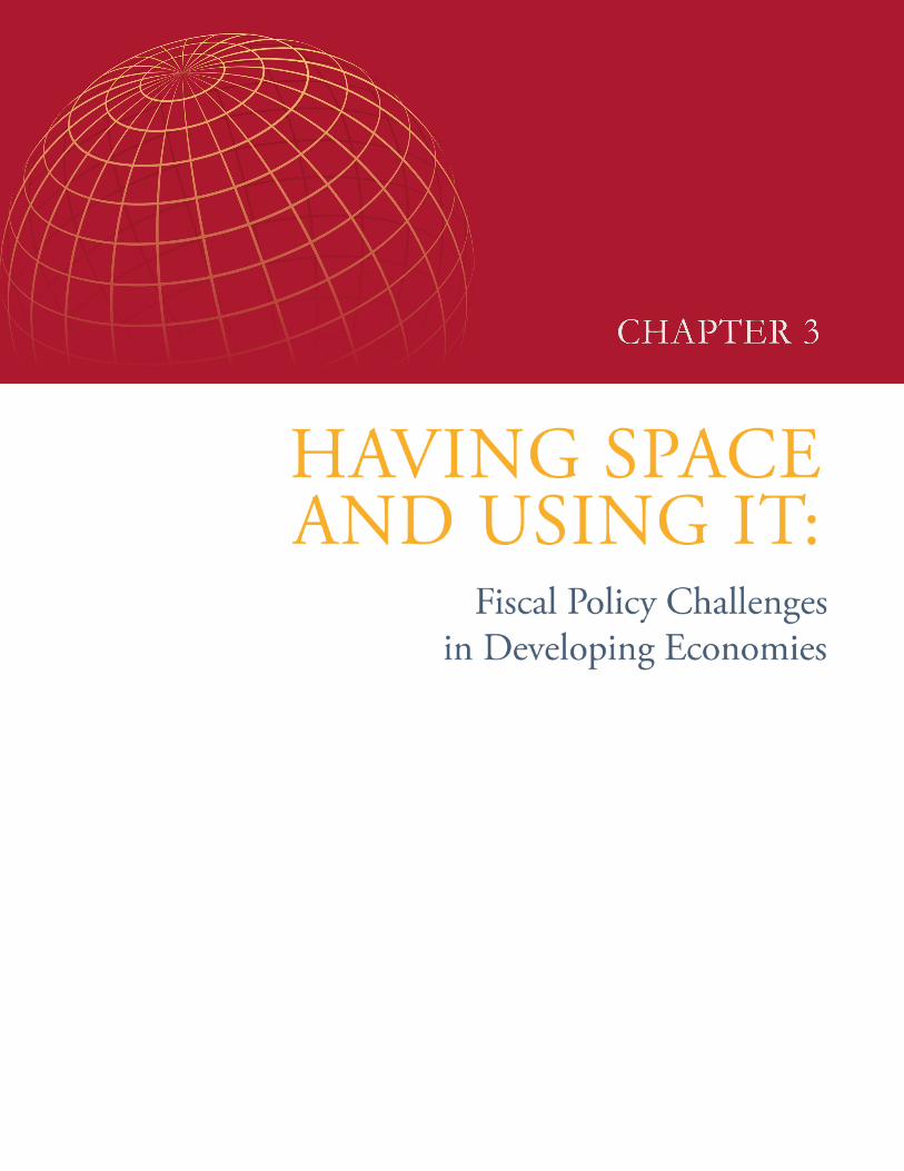

GLOBAL ECONOMIC PROSPECTS | January 2015 Chapter 3
121
Developing economies face downside risks to growth and prospects of
rising financing costs. In the event that these cause a cyclical slowdown,
policymakers may need to employ fiscal policy as a possible tool for
stimulus. But will developing economies be able to use fiscal policy
effectively? This chapter argues that fiscal space is essential for both the
availability and the effectiveness of fiscal policy. Developing economies
built fiscal space in the runup to the Great Recession of 2008–09,
which was then used for stimulus. This reflects a more general trend
over the past three decades, where availability of fiscal space has been
associated with increasingly countercyclical (or less procyclical) fiscal
policy. Wider fiscal space also appears to make fiscal policy more
effective. However, fiscal space has shrunk since the Great Recession
and has not returned to pre-crisis levels. Thus, developing economies
need to rebuild buffers at a pace appropriate to country-specific
conditions. For many countries, soft oil prices provide a window of
opportunity to implement subsidy reforms that help build fiscal space
while, at the same time, removing long-standing distortions. Over the
medium-term, credible and well-designed institutional arrangements,
such as fiscal rules, stabilization funds, and medium-term expenditure
frameworks, can help build fiscal space and strengthen policy outcomes.1
Introduction
Growth in developing economies has slowed in recent
years and significant downside risks remain, including
slowdowns in major trading partners. In addition,
financing costs are expected to rise from the current
exceptionally low levels when monetary policy
normalization gets under way in some advanced
economies. Tightening of global financial conditions and
bouts of financial market volatility might cause
slowdowns or reversals of capital inflows.2 Since the risk
to capital flows can constrain monetary policy in
developing economies, the option of fiscal policy as a
countercyclical tool becomes particularly important.3
How effective will fiscal policy be in supporting activity
in developing economies in the event of a downturn?
This question is the main focus of the chapter.
There are two related prerequisites for fiscal policy to be
useful. First, availability: governments need to have the
necessary fiscal space to implement countercyclical
measures. Second, effectiveness: countercyclical fiscal policy
has to be actually effective in raising the level of
economic activity.4 This chapter draws policy lessons by
analyzing the historical experience of developing
economies and answering the following questions:
How has fiscal space evolved over time?
Have developing economies “graduated” from the
procyclicality of fiscal policy during the 1980s?
Has greater fiscal space supported more effective
fiscal policy?
What institutional arrangements might strengthen
fiscal space and policy outcomes, drawing lessons
from country experiences?
What objectives with respect to fiscal space should
policymakers pursue in the current environment?
The focus here is on Emerging Market Economies
(EMEs) and Frontier Market Economies (FMEs) that are
able to tap international capital markets.5 The chapter
also briefly explores the role of fiscal policy in stimulating
activity in Low Income Countries (LICs) that depend on
concessional finance.
The chapter reports four main findings:
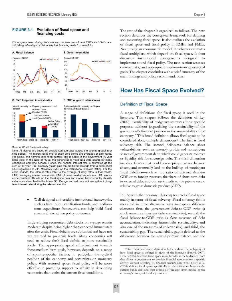
During the 2000s, in the runup to the Great
Recession of 2008–09, EMEs and FMEs built fiscal
space by reducing debt and closing deficits (Figure
3.1). To support activity during the Great Recession,
this space was used for fiscal stimulus. Deficits rose
and have remained elevated as EMEs and FMEs have
taken advantage of historically low interest rates.
Fiscal policy in EMEs and FMEs has become more
countercyclical (or less procyclical) since the 1980s, as
most clearly demonstrated during the Great Recession.
Wider fiscal space is associated with more effective
fiscal policy in developing economies: fiscal multipliers
tend to be larger in countries with greater fiscal space.
1This chapter is prepared by a team led by Ayhan Kose and Fran-ziska Ohnsorge, and including S. Amer Ahmed, Raju Huidrom, Sergio Kurlat, and Jamus J. Lim, with contributions from Israel Osorio-Rodarte and Nao Sugawara, as well as consultancy support from Rapha-el Espinoza, Ugo Panizza, and Carlos Végh.
2For a discussion on the potential impact of monetary policy nor-malization on growth and capital inflows in developing economies, see World Bank (2014a) and IMF (2014a).
3Countercyclicality of fiscal policy refers to an increase in govern-ment consumption or cut in taxes during downturns to support eco-nomic activity. In the empirical analysis, countercyclicality is defined as a negative and statistically significant response of government consump-tion to exogenous movements in GDP, as inferred from an econometric model. The chapter also examines countercyclicality in terms of negative and statistically significant correlations between the cyclical components of government consumption and GDP. See Technical Annex for details.
4The changing nature of fiscal policy, its availability, and effective-ness in advanced and developing economies have received attention in recent research. Vegh and Vuletin (2013) show how fiscal policy has become increasingly countercyclical in Latin America. Ilzetzki et al (2013) and Auerbach and Gorodnichenko (2012a) explore the effective-ness of fiscal policy in various samples of advanced economies and large emerging markets. Kraay (2012) and Eden and Kraay (2014) ex-amine the impact of fiscal policy in low-income countries.
5See Annex 3B for details on country classification.
GLOBAL ECONOMIC PROSPECTS | January 2015 Chapter 3
122
Well-designed and credible institutional frameworks,
such as fiscal rules, stabilization funds, and medium-
term expenditure frameworks, can help build fiscal
space and strengthen policy outcomes.
In developing economies, debt stocks on average remain
moderate despite being higher than expected immediately
after the crisis. Fiscal deficits are substantial and have not
yet returned to pre-crisis levels. Many economies will
need to reduce their fiscal deficits to more sustainable
levels. The appropriate speed of adjustment towards
these medium-term goals, however, depends on a range
of country-specific factors, in particular the cyclical
position of the economy and constraints on monetary
policy. With restored space, fiscal policy will be more
effective in providing support to activity in developing
economies than under the current fiscal conditions.
The rest of the chapter is organized as follows. The next
section describes the conceptual framework for defining
and measuring fiscal space. It also outlines the evolution
of fiscal space and fiscal policy in EMEs and FMEs.
Next, using an econometric model, the chapter estimates
fiscal multipliers, which depend on fiscal space. It then
discusses institutional arrangements designed to
implement sound fiscal policy. The next section assesses
current risks, and appropriate medium-term operational
goals. The chapter concludes with a brief summary of the
main findings and policy recommendations.
How Has Fiscal Space Evolved?
Definition of Fiscal Space
A range of definitions for fiscal space is used in the
literature. This chapter follows the definition of Ley
(2009): “availability of budgetary resources for a specific
purpose…without jeopardizing the sustainability of the
government’s financial position or the sustainability of the
economy.” This broad definition allows fiscal space to be
considered along multiple dimensions.6 The first is fiscal
solvency risk. The second delineates balance sheet
vulnerabilities, such as maturity profile and nonresident
shares of government debt, which could generate rollover
or liquidity risk for sovereign debt. The third dimension
involves factors that could stress private sector balance
sheets, and eventually lead to the buildup of contingent
fiscal liabilities—such as the ratio of external debt-to-
GDP or to foreign reserves, the share of short-term debt
in external debt, and domestic credit to the private sector
relative to gross domestic product (GDP).
In line with the literature, this chapter tracks fiscal space
mainly in terms of fiscal solvency. Fiscal solvency risk is
measured in three alternative ways to capture different
elements: first, the government debt-to-GDP ratio (a
stock measure of current debt sustainability); second, the
fiscal balance-to-GDP ratio (a flow measure of debt
accumulation, indicating future debt sustainability, and
also one of the measures of rollover risk); and third, the
sustainability gap. The sustainability gap is defined as the
difference between the actual primary balance and the
6This multidimensional definition helps address the ambiguity of how fiscal space is defined in much of the literature (Perotti, 2007). Heller (2005) describes fiscal space more broadly as the budgetary room that allows a government to provide financial resources for a specific activity without affecting its financial sustainability while Ostry et al. (2010) defines fiscal space specifically as the difference between the current public debt and their estimate of the debt limit implied by the economy’s history of fiscal adjustments.
Evolution of fiscal space and financing costs
Fiscal space used during the crisis has not been rebuilt and EMEs and FMEs are still taking advantage of historically low financing costs to run deficits.
FIGURE 3.1
A. Fiscal balance
-6
-5
-4
-3
-2
-1
0
1
2
3
1996 99 02 05 08 11 14
EME FME LICPercent of GDP
D. FME long-term interest rates
0
2
4
6
8
10
12
14
16
1997-2000 2001-05 2006-10 2011-14
Estimated yield to maturity on 10-year
government bond, percent
C. EME long-term interest rates
0
2
4
6
8
10
12
14
16
18
1997-2000 2001-05 2006-10 2011-14
Russian Crisis
(October 1998)
Dot-Com bubble
crash (March 2000)
Global Crisis
(October
2008)
Yield to maturity on 10-year government bond,
percent
B. Government debt
0
20
40
60
80
100
120
140
1996 99 02 05 08 11 14
EME FME LIC
Percent of GDP
Source: World Bank estimates.
Note: All figures are based on unweighted averages across the country grouping or time period. The interest rates over a given time period are averages of daily rates. For EMEs, the nominal long-term interest rate is equal to the government 10-year bond yield. In the case of FMEs, the generic bond yield data were sparse for many economies and time periods. Hence, the nominal interest rate is estimated as the sum of 10-year U.S. Treasury yields plus the predicted spreads from a fixed-effect OLS regression of J.P. Morgan’s EMBI on the Institutional Investor Rating. For the crisis periods, the interest rates refer to the average of daily rates in that month. EME: emerging market economies; FME: frontier market economies; LIC: low in-come countries. Details on the fiscal space data and market based country classifi-cations are described in the Annex 3B. Orange and red bars indicate spikes in long-term interest rates during the relevant months.
GLOBAL ECONOMIC PROSPECTS | January 2015 Chapter 3
123
3.6 percent of GDP in 2009 and 1.2 percent of GDP in
2010. Korea’s surplus has diminished since then and debt
is now almost 38 percent of GDP. Similarly, China had a
fiscal surplus in 2007, and government debt that was just
one-fifth of GDP. Following a stimulus package
equivalent to 12.5 percent of GDP in 2008, China ran
fiscal deficits from 2008 to 2010. Government debt rose
to more than 50 percent of GDP by 2010.10 Both
economies succeeded in preventing a contraction in real
GDP, despite the sharp downturn in the global economy.
Space and Policy during Contractions
China and Korea were particularly pronounced examples
of a broader pattern among EMEs and FMEs. Many
implemented countercyclical fiscal policy during the Great
Recession, but not all avoided GDP contractions. To
analyze fiscal policy responses during the Great Recession
as well as in past crises, the chapter conducts an event
study that identifies 101 episodes of sharp annual GDP
contractions in 157 advanced and developing economies
since 1990 (see Annex 3A for details). A country is
considered to have experienced a contraction event if its
GDP growth in a given year fulfills two conditions: first,
growth is negative (i.e., a contraction), and second,
growth is more than one standard deviation below the
average growth that the economy experienced over 1990–
2013. These criteria yielded 51 economies in the sample
that experienced a contraction during the Great
Recession, of which 21 were EMEs or FMEs.11
During the Great Recession, EMEs and FMEs used the
wider fiscal space they had accumulated during the
preceding years to allow automatic stabilizers to operate
and to implement larger fiscal stimulus than in earlier
contractions. Structural balances, which measure the
fiscal policy stance, declined sharply as economies
entered severe contractions (Figure 3.4).12 During both
event samples, fiscal space deteriorated following the
stimulus, reflected in an increase in government debt.
Government debt evolved differently across the two
samples, likely as a result of different exchange rate
movements and financial sector support programs.
7The debt stabilizing primary balance is defined as the primary balance that allows debt to converge to a target debt-to-GDP ratio. This is assumed to be the median stock of public debt as a share of a GDP for a given country grouping. The primary balance is the fiscal balance net of interest expense. Throughout this chapter, government debt refers to gross general government debt unless otherwise specified. See Annex 3B for additional details.
8As of 2014, 35 countries have reached the HIPC completion point and are eligible for assistance under the initiative, of which six are FMEs and 22 are LICs (IMF, 2014b). The most recent assessment of debt relief costs by the IMF (2013) determined that $126 billion has been committed under these initiatives to the 35 HIPC completion point countries, with another $442 million committed to Chad (an interim HIPC country), Cambodia, and Tajikistan. The latter two coun-tries are non-HIPC.
9See Eskesen (2009), Arbatli et al. (2010), and Fardoust, Lin, and Luo (2012) for a detailed discussion.
debt-stabilizing primary balance, which depends on the
target debt-to-GDP ratio to be achieved in the long run,
the interest rate, and growth.7 This last measure
recognizes that debt sustainability depends on output
growth and interest rates, as well as on outstanding debt
and deficits. In addition to these measures of fiscal
solvency risk, the chapter briefly discusses some aspects
of balance-sheet vulnerabilities and private-sector debt.
Evolution of Space during the 2000s
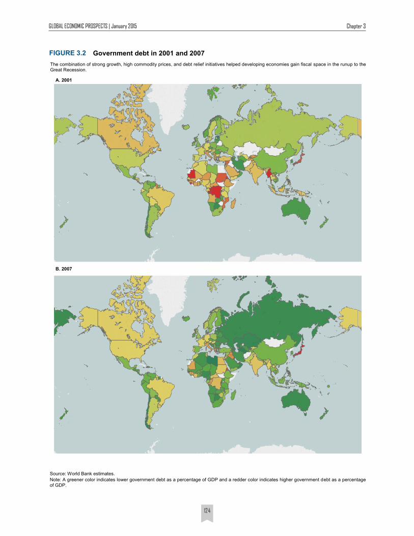
Between 2001 and 2007, in the runup to the Great
Recession, fiscal space widened for much of the
developing world, with government debt ratios falling and
fiscal deficits closing (Figures 3.1 and 3.2). Three factors
contributed to these changes. First, there was rapid
growth, with government revenues in commodity
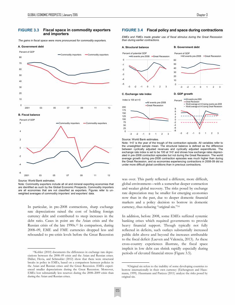
exporting economies bolstered by high and rising prices
(Figure 3.3). This coincided with a period of increasing
graduation of developing economies’ fiscal policy from
earlier procyclicality to more recent countercyclicality.
Second, debt relief initiatives, such as the Heavily
Indebted Poor Countries (HIPC) Initiative and
Multilateral Debt Relief Initiative (MDRI), helped to
reduce debt sharply in many FMEs and LICs.8 As a result,
most developing economies consolidated their finances in
the early 2000s. Third, institutional arrangements in
developing economies allowed for improvements in debt
management, which also contributed to the reduction in
debt-to-GDP ratios (Anderson, Silva and Valendia-
Rubiano, 2011; Frankel, Vegh, and Vuletin, 2013).
During the Great Recession, fiscal space narrowed as
economies implemented fiscal stimulus.9 For example, the
Republic of Korea boasted wide fiscal space in 2007, when
government debt was a third of GDP, and fiscal balance
was in surplus. In response to the crisis, the government
implemented two fiscal stimulus packages, amounting to
10The buildup of general government debt reflected a substantial expansion in local government off-balance sheet lending (World Bank, 2013a, 2014b).
11More than 80 percent of advanced market countries (AMEs), a third of EMEs and FMEs, and less than a tenth of LICs experienced a contraction in 2008-09 in the sample of countries considered.
12In this chapter, the structural balance is defined as the difference between cyclically-adjusted revenues and cyclically-adjusted expendi-tures. It thus removes the cycle-induced component of taxes and ex-penditures, such as social safety nets. See Statistical Annex for addition-al details.
GLOBAL ECONOMIC PROSPECTS | January 2015 Chapter 3
124
Source: World Bank estimates.
Note: A greener color indicates lower government debt as a percentage of GDP and a redder color indicates higher government debt as a percentage of GDP.
Government debt in 2001 and 2007 FIGURE 3.2
The combination of strong growth, high commodity prices, and debt relief initiatives helped developing economies gain fiscal space in the runup to the Great Recession.
A. 2001
B. 2007
GLOBAL ECONOMIC PROSPECTS | January 2015 Chapter 3
125
was over. This partly reflected a different, more difficult,
global environment—with a somewhat deeper contraction
and weaker global recovery. The risks posed by exchange
rate depreciation may be smaller for emerging economies
now than in the past, due to deeper domestic financial
markets and a policy decision to borrow in domestic
currency, thus reducing “original sin.”14
In addition, before 2008, some EMEs suffered systemic
banking crises which required governments to provide
heavy financial support. Though typically not fully
reflected in deficits, such outlays substantially increased
public debt above and beyond the increases attributable
to the fiscal deficit (Laeven and Valencia, 2013). As these
cross-country experiences illustrate, the fiscal space
implicit in low debt can shrink rapidly especially during
periods of elevated financial stress (Figure 3.5). 13Kohler (2010) documents the differences in exchange rate depre-
ciations between the 2008–09 crisis and the Asian and Russian crises. Didier, Hevia, and Schmukler (2012) show that there were structural breaks in policy in EMEs, based on a comparison between policies in the Asian and Russian crises and the Great Recession. EMEs experi-enced smaller depreciations during the Great Recession. Moreover, EMEs lost substantially less reserves during the 2008–2009 crisis than during the Asian and Russian crises.
In particular, in pre-2008 contractions, sharp exchange
rate depreciations raised the cost of holding foreign
currency debt and contributed to steep increases in the
debt ratio. Cases in point are the Asian crisis and the
Russian crisis of the late 1990s.13 In comparison, during
2008–09, EME and FME currencies dropped less and
rebounded to pre-crisis levels before the Great Recession
The gains in fiscal space were more pronounced for commodity exporters.
Fiscal space in commodity exporters and importers
FIGURE 3.3
Source: World Bank estimates.
Note: Commodity exporters include all oil and mineral exporting economies that are identified as such by the Global Economic Prospects. Commodity importers are all economies that are not classified as exporters. Figures refer to un-weighted averages of commodity importers’ and exporters’ data.
A. Government debt
0
10
20
30
40
50
60
70
80
2001 03 05 07 09 11 13
Commodity importers Commodity exporters
Percent of GDP
B. Fiscal balance
-6
-4
-2
0
2
4
6
2001 03 05 07 09 11 13
Commodity importers Commodity exporters
Percent of GDP
14Original sin refers to the inability of some developing countries to borrow internationally in their own currency (Eichengreen and Haus-mann, 1999). Hausmann and Panizza (2011) analyze the risks posed by original sin.
Source: World Bank estimates.
Note: ‘t=0’ is the year of the trough of the contraction episode. All variables refer to the unweighted sample mean. The structural balance is defined as the difference between cyclically adjusted revenues and cyclically adjusted expenditures. The exchange rate index is set to be 100 at ‘t=0’ and shows how exchange rates depreci-ated in pre-2008 contraction episodes but not during the Great Recession. The world average growth during pre-2008 contraction episodes was much higher than during the Great Recession, and so economies experiencing contractions in 2008-09 did so
under more difficult global conditions than in previous contractions.
FIGURE 3.4
EMEs and FMEs made greater use of fiscal stimulus during the Great Recession than during earlier contractions.
A. Structural balance
-5
-4
-3
-2
-1
0
-3 -2 -1 0 1 2 3
All events pre-2008 Great Recession
Percent of potential GDP
C. Exchange rate index
0
25
50
75
100
125
150
175
200
-3 -2 -1 0 1 2 3
All events pre-2008
Great Recession
Index is 100 at t=0
Fiscal policy and space during contractions
D. GDP growth
B. Government debt
0
10
20
30
40
50
60
-3 -2 -1 0 1 2 3
All events pre-2008 Great Recession
Percent of GDP
-8
-6
-4
-2
0
2
4
6
8
-3 -2 -1 0 1 2 3
All events pre-2008Great RecessionWorld average at t=0 during events pre-2008World average at t=0 during Great Recession
Percent
GLOBAL ECONOMIC PROSPECTS | January 2015 Chapter 3
126
While the sample is too small to compute estimates for
EMEs and FMEs separately, correlations between real GDP
and real government consumption also suggest a similarity
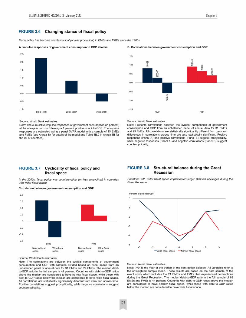
between the two groups. High procyclicality between 1980
and 1999, broadly turned to acyclicality in EMEs in the early
2000s, and to countercyclicality after the Great Recession.
This evolution of fiscal cyclicality can be attributed to several
factors, including improvements in policies, institutions, and
enhanced financial market access.16
The move to less procyclical fiscal policy has also been
associated with greater fiscal space. Throughout the
2000s, procyclicality was less pronounced in economies
with wide fiscal space (Figure 3.7). During the Great
Recession, economies with government debt below 40
percent of GDP (implying wider fiscal space) were able to
implement greater fiscal stimulus than more indebted
governments (with narrower space) (Figure 3.8). Fiscal
policy in LICs has remained mostly acyclical reflecting the
severe budgetary constraints they often face (Box 3.1).17
Overall, the evidence presented in this section suggests
that fiscal space matters for a government’s ability to
implement countercyclical fiscal policy. The next section
explores the importance of space for policy effectiveness.
Does Greater Space Tend to Support More Effective Fiscal Outcomes?
Countries with more ample fiscal space have used stimulus
more extensively during the Great Recession than those
with tighter space. But has this stimulus been more effective
at meeting the goal of supporting activity? Space may affect
the effectiveness of fiscal policy through two channels.
Interest rate channel: When fiscal space is narrow,
expansionary policy can increase lenders’ perceptions
15These responses are estimated using a vector autoregressive mod-el (VAR) with a pooled sample of EMEs and FMEs. See Technical Annex for details of the VAR model.
16Frankel, Végh, and Vuletin (2013) emphasize the importance of improvements in institutional quality for the changes in cyclicality. Calderon and Schmidt-Hebbel (2008) and World Bank (2013b) discuss the im-portance of greater credibility of fiscal policies and deepening domestic financial markets.
17World Bank (2013b) offers explanations of the procyclical bias of fiscal policy in developing countries. Developing countries have generally procyclical access to capital markets, and governments must therefore make spending cuts during downturns, when they are less able or unable to bor-row. During upswings, governments are often under political pressure to spend the higher revenues.
Have Developing Economies Graduated from Procyclicality?
There are several measures of the stance of fiscal policy.
This chapter employs two that are commonly used in the
literature: the structural balance and government
consumption. The structural balance strips from the
overall balance the rise and fall of revenues (such as the
cycle-induced component of income taxes) and
expenditures (especially social benefits) that can be
attributed to the business cycle. The other measure,
government consumption expenditures, which are mainly
government wages and outlays on goods and services,
provides a narrower definition of the fiscal policy stance,
but one that is more readily comparable across economies
and not subject to the uncertainty surrounding the
accuracy of cyclical adjustments, for example the
uncertainty about the cyclical income elasticity of tax
revenues or the size of the output gap. On either measure,
fiscal policy was significantly more expansionary during the
Great Recession than during earlier contraction episodes.
Structural balances widened, on average among EMEs and
FMEs, by 4 percentage points of GDP during the Great
Recession, whereas they tightened in earlier contractions.
The buildup of fiscal space during the global expansion of
the early 2000s, and its use during the Great Recession
suggest that fiscal policy has become less procyclical in
developing economies. Estimated responses of government
consumption to GDP shocks indeed show that fiscal policy
has become less procyclical since the 1990s, and more
countercyclical since the Great Recession (Figure 3.6).15
Government debt in select crises FIGURE 3.5
Debt can rise very quickly during a crisis episode.
Source: World Bank estimates.
Note: Central government debt is used for Indonesia. The others refer to general government debt.
1996
1996
2007
2007
1998
1998
2009
2009
0
10
20
30
40
50
60
70
Indonesia Thailand Ireland Latvia
Percent of GDP
GLOBAL ECONOMIC PROSPECTS | January 2015 Chapter 3
127
Structural balance during the Great Recession
FIGURE 3.8
Countries with wider fiscal space implemented larger stimulus packages during the Great Recession.
Source: World Bank estimates.
Note: ‘t=0’ is the year of the trough of the contraction episode. All variables refer to the unweighted sample mean. These results are based on the data sample of the event study which includes the 21 EMEs and FMEs that experienced contractions during the Great Recession. The median debt-to-GDP ratio in the full sample of 63 EMEs and FMEs is 44 percent. Countries with debt-to-GDP ratios above the median are considered to have narrow fiscal space, while those with debt-to-GDP ratios below the median are considered to have wide fiscal space.
-5
-4
-3
-2
-1
0
-3 -2 -1 0 1 2 3
Wide fiscal space Narrow fiscal space
Percent of potential GDP
Cyclicality of fiscal policy and fiscal space
FIGURE 3.7
In the 2000s, fiscal policy was countercyclical (or less procyclical) in countries with wider fiscal space.
Source: World Bank estimates.
Note: The correlations are between the cyclical components of government consumption and GDP with samples divided based on fiscal space from an unbalanced panel of annual data for 31 EMEs and 29 FMEs. The median debt-to-GDP ratio in the full sample is 44 percent. Countries with debt-to-GDP ratios above the median are considered to have narrow fiscal space, while those with debt-to-GDP ratios below the median are considered to have wide fiscal space. All correlations are statistically significantly different from zero and across time. Positive correlations suggest procyclicality, while negative correlations suggest countercyclicality.
-0.6
-0.4
-0.2
0
0.2
0.4
0.6
0.8
EME FME
Narrow fiscal
space
Wide fiscal
space
Wide fiscal
space
Narrow fiscal
space
Correlation between government consumption and GDP
Changing stance of fiscal policy FIGURE 3.6
Fiscal policy has become countercyclical (or less procyclical) in EMEs and FMEs since the 1980s.
Source: World Bank estimates.
Note: Presents correlations between the cyclical components of government consumption and GDP from an unbalanced panel of annual data for 31 EMEs and 29 FMEs. All correlations are statistically significantly different from zero and differences in correlations across time are also statistically significant. Positive responses (Panel A) and positive correlations (Panel B) suggest procyclicality, while negative responses (Panel A) and negative correlations (Panel B) suggest countercyclicality.
A. Impulse responses of government consumption to GDP shocks B. Correlations between government consumption and GDP
-1.0
-0.5
0.0
0.5
1.0
1.5
2.0
2.5
1980-1999 2000-2007 2008-2014
1980
-99
1980
-99
2000
-07 20
00-0
7
2008
-14
2008
-14
-1.5
-1.0
-0.5
0.0
0.5
1.0
1.5
EME FME
Source: World Bank estimates.
Note: The cumulative impulse responses of government consumption (in percent) at the one-year horizon following a 1 percent positive shock to GDP. The impulse responses are estimated using a panel SVAR model with a sample of 15 EMEs and FMEs (see Annex 3A for details of the model and Table 3B.2 in Annex 3B for the list of countries).
GLOBAL ECONOMIC PROSPECTS | January 2015 Chapter 3
128
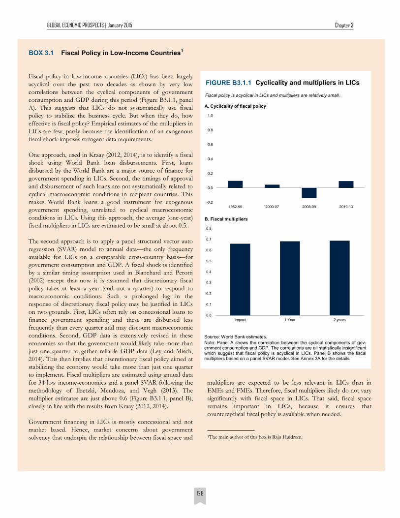
Fiscal Policy in Low-Income Countries1 BOX 3.1
Fiscal policy in low-income countries (LICs) has been largely
acyclical over the past two decades as shown by very low
correlations between the cyclical components of government
consumption and GDP during this period (Figure B3.1.1, panel
A). This suggests that LICs do not systematically use fiscal
policy to stabilize the business cycle. But when they do, how
effective is fiscal policy? Empirical estimates of the multipliers in
LICs are few, partly because the identification of an exogenous
fiscal shock imposes stringent data requirements.
One approach, used in Kraay (2012, 2014), is to identify a fiscal
shock using World Bank loan disbursements. First, loans
disbursed by the World Bank are a major source of finance for
government spending in LICs. Second, the timings of approval
and disbursement of such loans are not systematically related to
cyclical macroeconomic conditions in recipient countries. This
makes World Bank loans a good instrument for exogenous
government spending, unrelated to cyclical macroeconomic
conditions in LICs. Using this approach, the average (one-year)
fiscal multipliers in LICs are estimated to be small at about 0.5.
The second approach is to apply a panel structural vector auto
regression (SVAR) model to annual data—the only frequency
available for LICs on a comparable cross-country basis—for
government consumption and GDP. A fiscal shock is identified
by a similar timing assumption used in Blanchard and Perotti
(2002) except that now it is assumed that discretionary fiscal
policy takes at least a year (and not a quarter) to respond to
macroeconomic conditions. Such a prolonged lag in the
response of discretionary fiscal policy may be justified in LICs
on two grounds. First, LICs often rely on concessional loans to
finance government spending and these are disbursed less
frequently than every quarter and may discount macroeconomic
conditions. Second, GDP data is extensively revised in these
economies so that the government would likely take more than
just one quarter to gather reliable GDP data (Ley and Misch,
2014). This then implies that discretionary fiscal policy aimed at
stabilizing the economy would take more than just one quarter
to implement. Fiscal multipliers are estimated using annual data
for 34 low income-economies and a panel SVAR following the
methodology of Ilzetzki, Mendoza, and Vegh (2013). The
multiplier estimates are just above 0.6 (Figure B3.1.1, panel B),
closely in line with the results from Kraay (2012, 2014).
Government financing in LICs is mostly concessional and not
market based. Hence, market concerns about government
solvency that underpin the relationship between fiscal space and 1The main author of this box is Raju Huidrom.
Source: World Bank estimates.
Note: Panel A shows the correlation between the cyclical components of gov-ernment consumption and GDP. The correlations are all statistically insignificant which suggest that fiscal policy is acyclical in LICs. Panel B shows the fiscal multipliers based on a panel SVAR model. See Annex 3A for the details.
Cyclicality and multipliers in LICs FIGURE B3.1.1
Fiscal policy is acyclical in LICs and multipliers are relatively small.
A. Cyclicality of fiscal policy
B. Fiscal multipliers
-0.2
0.0
0.2
0.4
0.6
0.8
1.0
1982-99 2000-07 2008-09 2010-13
0.0
0.1
0.2
0.3
0.4
0.5
0.6
0.7
0.8
Impact 1 Year 2 years
multipliers are expected to be less relevant in LICs than in
EMEs and FMEs. Therefore, fiscal multipliers likely do not vary
significantly with fiscal space in LICs. That said, fiscal space
remains important in LICs, because it ensures that
countercyclical fiscal policy is available when needed.

GLOBAL ECONOMIC PROSPECTS | January 2015 Chapter 3
129
of sovereign credit risk. This raises sovereign bond
yields and hence, borrowing costs across the whole
economy (Corsetti et al., 2013; Bi, Shen, and Yang,
2014). This, in turn, crowds out private investment
and consumption. If the crowding out is sufficiently
strong, the net effect of expansionary fiscal policy on
output, that is, the size of the fiscal multiplier, may
be negligible or even negative.
Ricardian channel: When a government with narrow
fiscal space conducts a fiscal expansion, households
expect tax increases sooner than in an economy with
wide fiscal space (Perotti, 1999; Sutherland, 1997).
The perceived negative wealth effect encourages
households to cut consumption and save, thereby
weakening the impact of the policy on output.18
The effectiveness of fiscal policy is usually evaluated in
terms of the fiscal multiplier–the change in output for a
dollar increase in government consumption. The more
positive the multiplier, the more effective is policy. For
developing economies, the literature reports multipliers that
are small in size, and variable, ranging from -0.4 to 0.9 (Box
3.2). These estimates often refer to average multipliers, over
a whole range of macroeconomic conditions. Recent work
in the context of advanced economies has found that
multipliers vary significantly depending on macroeconomic
conditions and country characteristics: they tend to be
larger during recessions (Auerbach and Gorodnichenko,
2012a, 2012b), for economies using a fixed exchange rate
regime, and for economies with low debt (Ilzetzki,
Mendoza, and Vegh, 2013, based on pre-crisis data; Nickel
and Tudyka, 2013, for OECD economies).
To estimate fiscal multipliers for developing economies
that depend on fiscal space, this section employs an
Interacted Panel VAR (IPVAR) model (Towbin and
Weber, 2013). This allows model parameters, and hence
estimated fiscal multipliers, to interact with fiscal space.
Fiscal shocks are identified by assuming that discretionary
policy takes at least one quarter to respond to
macroeconomic conditions (Blanchard and Perotti, 2002).
The variables included in the model are government
consumption, GDP, current account balance, and real
18While crowding-out effects of fiscal policy, that operate via higher inter-est rates or future increase in taxes, have long been discussed in the literature, the emphasis in this chapter is that such crowding-out effects can be nonlinear and can depend on fiscal space. In particular, the nonlinearity pertains to investors’ perception of sovereign credit risk (interest rate channel) and house-holds’ expectation of future tax increases as fiscal space becomes narrow (Ricardian channel). The interest rate channel is less relevant for large advanced economies that are able to issue debt in their own currency (Krugman, 2011).
19This follows Ilzetzki, Mendoza, and Vegh (2013). 20Since data availability and comparability is limited for the EMEs and
FMEs included here, the analysis does not address the issue of spending composition, although this may be important. For instance, government spending on infrastructure and health has been shown to protect and strengthen social safety net programs, and result in long-run growth benefits (Berg et al., 2009; Kraay and Serven, 2013). Public infrastructure investment multipliers are often much larger than the public consumption multipliers (IMF, 2014c). The analysis here also does not cover automatic stabilizers which, at least in the case of OECD countries, has played a strong role in stabilizing output (Fatás and Mihov, 2012).
21Indeed, this fiscal space measure is not systematically wider during reces-sions than expansions in the sample of EMEs and FMEs. For example, the average fiscal deficit during recessions is 2.7 percent of GDP, which is very close to the deficits during expansions, 2.8 percent of GDP. Alternatively, the regression coefficients could be interacted with an additional dummy for reces-sions. However, this reduces the degrees of freedom significantly and results in imprecise estimates. The fiscal space measure also does not reflect exchange rate regimes—the proportion of fixed and flexible exchange rate regimes in the sample is roughly the same during periods of wide and narrow fiscal space.
22The multipliers presented here are the cumulative multipliers that take into account the persistence in the response of government con-sumption due to a fiscal shock. See Annex 3A for details.
effective exchange rates.19 The baseline results are based on
an unbalanced panel for 15 EMEs and FMEs (augmented
by 19 advanced economies in robustness exercises). The
data are quarterly, 1980:1–2014:1. Fiscal policy is proxied
by government consumption.20 The model estimates fiscal
multipliers as a function of fiscal space, which is proxied by
fiscal balances as percent of GDP, corresponding to a flow
measure. To control for endogeneity and to ensure that
fiscal balances do not systematically pick up business cycle
effects, lagged moving averages of fiscal balances are
employed.21
The results (Figure 3.9) suggest that the multipliers at the
one-year horizon are not much above zero when pre-
existing fiscal deficits leading up to the stimulus have been
high (narrow fiscal space), but are positive and significant
when there have been surpluses (wide fiscal space).22 The
multipliers at the two-year horizon are generally greater
than at the one-year horizon, suggesting that the effects
peak with some lag. At longer horizons, multipliers remain
near zero and statistically insignificant when fiscal space is
narrow, but can be as high as 1.8 when fiscal space is wide.
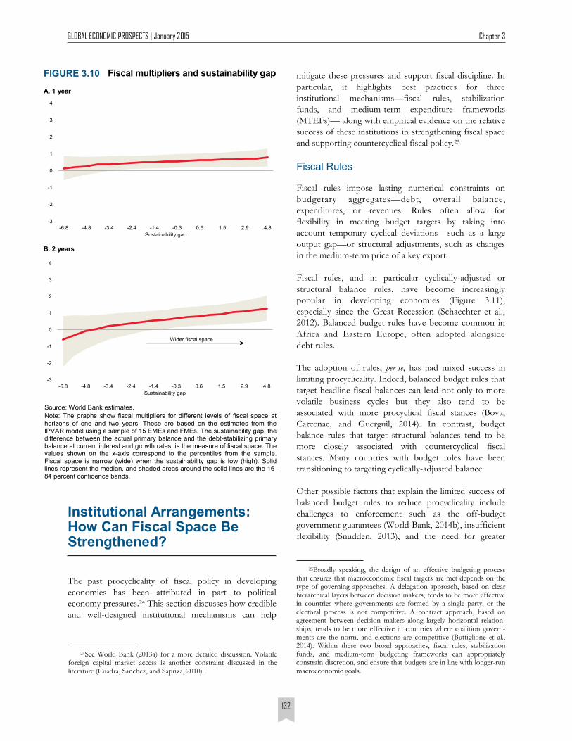
This result is qualitatively robust to alternative measures
of fiscal space. For example, the results for the multipliers
that use the sustainability gap as the gauge of fiscal space
also point to these conclusions (Figure 3.10). The results
are similar when government debt as percent of GDP is
used as the measure of fiscal space (see Annex 3A).
In addition to the baseline model above, two alternative
econometric models are used to examine robustness: a panel
Structural VAR (SVAR) as in Ilzetzki, Mendoza, and Vegh
(2013), and a local projections model as in Riera-Crichton, Vegh,
GLOBAL ECONOMIC PROSPECTS | January 2015 Chapter 3
130
1The main author of this box is Jamus J. Lim. 2Using tax revenues as the fiscal instrument first involves adjusting for the
cyclical or the automatic stabilizer component via elasticity estimates. One rea-son the chapter does not discuss revenue-based multipliers is that elasticity estimates tend to be unreliable for EMEs and FMEs.
What Affects the Size of Fiscal Multipliers?1 BOX 3.2
The size of fiscal multipliers depends on macroeconomic
conditions and country-specific features. While the chapter
examines how fiscal multipliers depend on fiscal space,
especially in the context of developing economies, this box
reviews additional aspects that have been important in
explaining the size of multipliers.
Conditions affecting multipliers
Fiscal multipliers depend on the phase of the business cycle:
they tend to be larger during recessions than during expansions
(Auerbach and Gorodnichenko, 2012a, 2012b). In theory, this is
attributed to a higher level of economic slack (Rendahl, 2012)
and a greater share of liquidity-constrained households
(Canzoneri et al., 2012) during economic downturns. The
effectiveness of fiscal policy also depends on monetary policy.
Monetary contraction, in response to expansionary fiscal policy
that increases inflation and output, blunts the effects of the fiscal
policy on output. Similarly, the effects of fiscal policy on output
are more pronounced when monetary policy is more
accommodative, especially when interest rates are at the zero
lower bound (Christiano, Eichenbaum, and Rebelo, 2011).
The effectiveness of fiscal policy also depends on country-
specific features. Fiscal multipliers tend to be larger in
economies with fixed exchange rates than in economies with
flexible exchange rates (Ilzetzki, Mendoza, and Vegh, 2013)
because, in fixed regimes, expansionary fiscal policy tends to
trigger some monetary accommodation. Fiscal multipliers are
also larger in less open economies because of lower leakages into
import demand.
Finally, the choice of the fiscal instrument matters. Revenue-
based fiscal multipliers tend to be lower (especially in the short
term) than expenditure-based multipliers. Expenditures tend to
affect aggregate demand directly, whereas changes in revenues
operate only indirectly and are subject to leakage. For example,
households may save a portion of tax cuts intended to stimulate
aggregate demand. Some caution is warranted here as recent
work has shown that cyclically adjusted tax revenues are not a
good proxy for tax policy. Riera-Crichton, Vegh and Vuletin
(2012) argue that using tax rates instead of tax revenues yields
considerably higher tax multipliers.
Empirical estimates
Empirical estimation of fiscal multipliers requires a strategy to
identify exogenous fiscal shocks. The one deployed in the
chapter relies on a timing assumption that discretionary fiscal
policy takes at least a quarter to respond to macroeconomic
conditions (Blanchard and Perotti, 2002). There are alternative
identification strategies deployed in the literature: the
narrative approach as in Ramey and Shapiro (1998) or
Guajardo, Leigh, and Pescatori (2014); forecast errors as in
Blanchard and Leigh (2013); or fluctuations in aid-related
financing approval used as instruments in Kraay (2012, 2014).
Fiscal multipliers can also be obtained from estimated
dynamic stochastic general equilibrium (DSGE) models
(Coenen et al., 2012). While empirical approaches yield
reduced-form estimates of fiscal multipliers, DSGE-based
estimates can capture deep structural features of the economy,
in particular the interactions between private-sector behavior
and policy parameters.
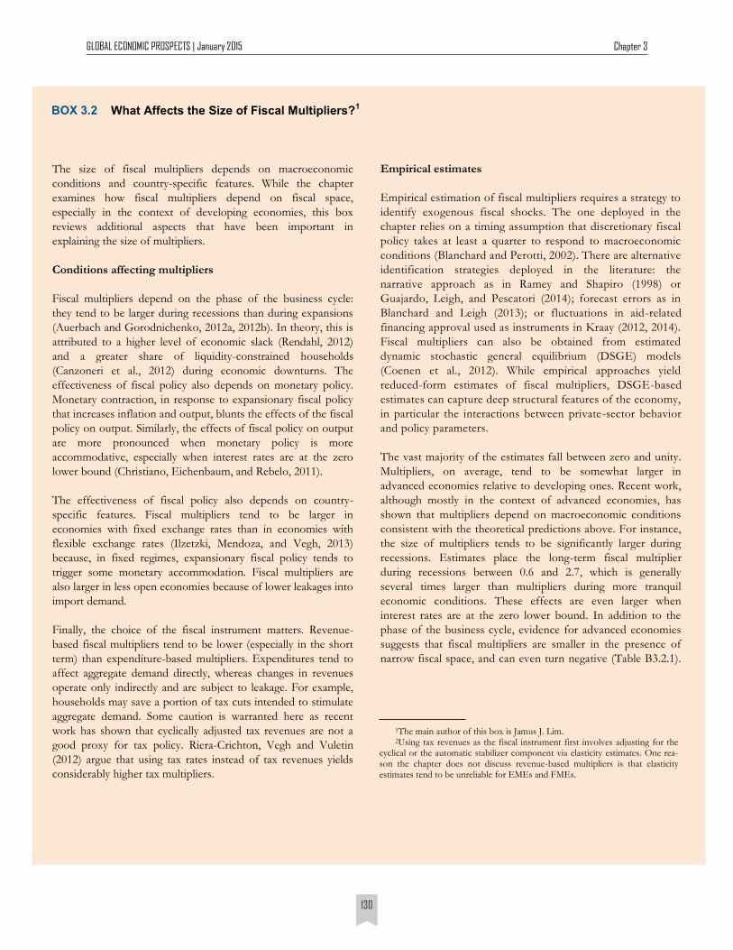
The vast majority of the estimates fall between zero and unity.
Multipliers, on average, tend to be somewhat larger in
advanced economies relative to developing ones. Recent work,
although mostly in the context of advanced economies, has
shown that multipliers depend on macroeconomic conditions
consistent with the theoretical predictions above. For instance,
the size of multipliers tends to be significantly larger during
recessions. Estimates place the long-term fiscal multiplier
during recessions between 0.6 and 2.7, which is generally
several times larger than multipliers during more tranquil
economic conditions. These effects are even larger when
interest rates are at the zero lower bound. In addition to the
phase of the business cycle, evidence for advanced economies
suggests that fiscal multipliers are smaller in the presence of
narrow fiscal space, and can even turn negative (Table B3.2.1).
GLOBAL ECONOMIC PROSPECTS | January 2015 Chapter 3
131
and Vuletin (2014).23 Although the precise estimates of the
multipliers differ, the results from the alternative models also
suggest that fiscal policy is more effective—fiscal multipliers are
higher—when pre-existing fiscal space leading up to the
stimulus is wide than when it is narrow (see Annex 3A).
In sum, the empirical evidence presented here suggests
that wider fiscal space is associated with more effective
fiscal policy in developing economies. This result holds
for different types of fiscal space measures using various
empirical approaches.
(continued) BOX 3.2
Fiscal multipliers: A review of studies
TABLE B3.2.1
Sources: World Bank compilation; Batini et al., (2014); Ilzetzki, Mendoza, and Vegh (2013); Mineshima, Poplawski-Ribeiro, and Weber (2014); and Ramey (2011). Notes: Estimates are for both government consumption and ex-penditure multipliers. Minimum and maximum estimates may refer to distinct studies and/or economies. Where available, short-term multipliers report the impact multiplier; otherwise the multiplier at the one-year horizon is used. Where available, long-term multipliers report the cumulative multiplier at the horizon of five years; other-wise the longest (generally three-year) horizon is used. The high-income and developing multipliers report linear estimates without state dependency. 1The upper-middle income estimates are skewed by the unusually large multiplier of China (2.8). Hence, China was excluded from the computation of the upper bound. 2Applies to zero lower bound for monetary policy rates. Multipliers depend heavily on the duration of the period in which the zero lower bound is binding; short-term (long-term) estimates reported here correspond to a zero lower bound of one (twelve) quarters. 3Fiscal space in these studies is usually measured in terms of the debt-to-GDP ratio: a high (low) debt-GDP ratio indicates fiscal space is narrow (wide).
Groups/ Feat uresSho rt - t erm
mult ip lier
Long- t erm
mult ip lier
Income g roup
Advanced economies -0.1 – 1.2 -1.1 – 1.8
Developing economies -0.4 – 0.6 -0.4 – 0.9
Upper-middle income1 0.0 – 0.6 -0.3 – 0.9
Lower-middle income -0.4 – 0.4 -0.4 – 0.0
Low income 0.2 – 0.5 -0.3 – 0.8
B usiness cycle
Expansion -0.9 – 1.4 -0.5 – 1.1
Recession 0.3 – 2.5 0.6 – 2.7
Zero lower bound2 2.3 – 3.7 1.0 – 4.0
F iscal space
Wide space3 0.0 – 1.1 -0.4 – 1.8
Narrow space -0.2 – 0.9 -3.0 – 1.3
23Details of these two models are provided in Annex 3A.
Fiscal multipliers by fiscal space FIGURE 3.9
Fiscal policy in EMEs and FMEs tends to be more effective when fiscal space is wider.
Source: World Bank estimates.
Note: The graphs show fiscal multipliers for different levels of fiscal space at hori-zons of one and two years. These are based on the estimates from the IPVAR model using a sample of 15 EMEs and FMEs. Fiscal balance as a percentage of GDP is the measure of fiscal space and the values shown on the x-axis correspond to the percentiles from the sample. Fiscal space is narrow (wide) when fiscal balanc-es are low (high). Solid lines represent the median, and shaded areas around the solid lines are the 16-84 percent confidence bands.
A. 1 year
B. 2 years
-1
0
1
2
3
-7.3 -5.4 -4.4 -3.8 -3.1 -2.7 -1.9 -1.1 -0.5 1.9
Fiscal balances as percent of GDP
Wider fiscal space
-1
0
1
2
3
-7.3 -5.4 -4.4 -3.8 -3.1 -2.7 -1.9 -1.1 -0.5 1.9
Fiscal balances as percent of GDP
GLOBAL ECONOMIC PROSPECTS | January 2015 Chapter 3
132
24See World Bank (2013a) for a more detailed discussion. Volatile foreign capital market access is another constraint discussed in the literature (Cuadra, Sanchez, and Sapriza, 2010).
mitigate these pressures and support fiscal discipline. In
particular, it highlights best practices for three
institutional mechanisms—fiscal rules, stabilization
funds, and medium-term expenditure frameworks
(MTEFs)— along with empirical evidence on the relative
success of these institutions in strengthening fiscal space
and supporting countercyclical fiscal policy.25
Fiscal Rules
Fiscal rules impose lasting numerical constraints on
budgetary aggregates—debt, overall balance,
expenditures, or revenues. Rules often allow for
flexibility in meeting budget targets by taking into
account temporary cyclical deviations—such as a large
output gap—or structural adjustments, such as changes
in the medium-term price of a key export.
Fiscal rules, and in particular cyclically-adjusted or
structural balance rules, have become increasingly
popular in developing economies (Figure 3.11),
especially since the Great Recession (Schaechter et al.,
2012). Balanced budget rules have become common in
Africa and Eastern Europe, often adopted alongside
debt rules.
The adoption of rules, per se, has had mixed success in
limiting procyclicality. Indeed, balanced budget rules that
target headline fiscal balances can lead not only to more
volatile business cycles but they also tend to be
associated with more procyclical fiscal stances (Bova,
Carcenac, and Guerguil, 2014). In contrast, budget
balance rules that target structural balances tend to be
more closely associated with countercyclical fiscal
stances. Many countries with budget rules have been
transitioning to targeting cyclically-adjusted balance.
Other possible factors that explain the limited success of
balanced budget rules to reduce procyclicality include
challenges to enforcement such as the off-budget
government guarantees (World Bank, 2014b), insufficient
flexibility (Snudden, 2013), and the need for greater
Fiscal multipliers and sustainability gap FIGURE 3.10
Source: World Bank estimates.
Note: The graphs show fiscal multipliers for different levels of fiscal space at horizons of one and two years. These are based on the estimates from the IPVAR model using a sample of 15 EMEs and FMEs. The sustainability gap, the difference between the actual primary balance and the debt-stabilizing primary balance at current interest and growth rates, is the measure of fiscal space. The values shown on the x-axis correspond to the percentiles from the sample. Fiscal space is narrow (wide) when the sustainability gap is low (high). Solid lines represent the median, and shaded areas around the solid lines are the 16-84 percent confidence bands.
A. 1 year
B. 2 years
-3
-2
-1
0
1
2
3
4
-6.8 -4.8 -3.4 -2.4 -1.4 -0.3 0.6 1.5 2.9 4.8
Sustainability gap
-3
-2
-1
0
1
2
3
4
-6.8 -4.8 -3.4 -2.4 -1.4 -0.3 0.6 1.5 2.9 4.8
Sustainability gap
Wider fiscal space
Institutional Arrangements: How Can Fiscal Space Be Strengthened?
The past procyclicality of fiscal policy in developing
economies has been attributed in part to political
economy pressures.24 This section discusses how credible
and well-designed institutional mechanisms can help
25Broadly speaking, the design of an effective budgeting process that ensures that macroeconomic fiscal targets are met depends on the type of governing approaches. A delegation approach, based on clear hierarchical layers between decision makers, tends to be more effective in countries where governments are formed by a single party, or the electoral process is not competitive. A contract approach, based on agreement between decision makers along largely horizontal relation-ships, tends to be more effective in countries where coalition govern-ments are the norm, and elections are competitive (Buttiglione et al., 2014). Within these two broad approaches, fiscal rules, stabilization funds, and medium-term budgeting frameworks can appropriately constrain discretion, and ensure that budgets are in line with longer-run macroeconomic goals.
GLOBAL ECONOMIC PROSPECTS | January 2015 Chapter 3
133
transparency and improved measurement in the
estimation of structural balances. Rules are best when
simply defined and supported by surveillance
arrangements, respected by the government, yet operated
by a non-government agency (Frankel, 2011). Chile’s use
of a technical fiscal council and a fiscal rule that targets a
fixed structural balance is a good example of a well-
designed, credible, and successfully operated fiscal rule
(Box 3.3). Such agencies have legal guarantees for
independence, highly qualified professional staff, and
assured financing (Debrun and Schaechter, 2014).
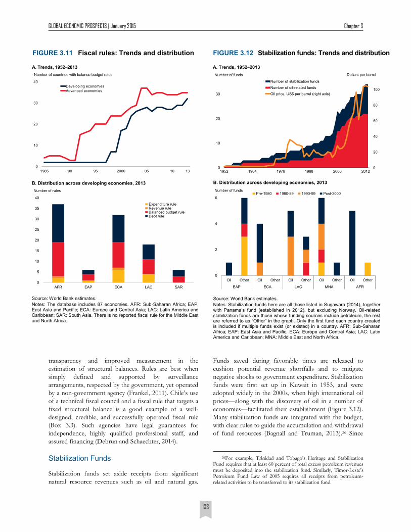
Stabilization Funds
Stabilization funds set aside receipts from significant
natural resource revenues such as oil and natural gas.
Funds saved during favorable times are released to
cushion potential revenue shortfalls and to mitigate
negative shocks to government expenditure. Stabilization
funds were first set up in Kuwait in 1953, and were
adopted widely in the 2000s, when high international oil
prices—along with the discovery of oil in a number of
economies—facilitated their establishment (Figure 3.12).
Many stabilization funds are integrated with the budget,
with clear rules to guide the accumulation and withdrawal
of fund resources (Bagnall and Truman, 2013).26 Since
26For example, Trinidad and Tobago’s Heritage and Stabilization Fund requires that at least 60 percent of total excess petroleum revenues must be deposited into the stabilization fund. Similarly, Timor-Leste’s Petroleum Fund Law of 2005 requires all receipts from petroleum-related activities to be transferred to its stabilization fund.
Fiscal rules: Trends and distribution FIGURE 3.11
Source: World Bank estimates.
Notes: The database includes 87 economies. AFR: Sub-Saharan Africa; EAP: East Asia and Pacific; ECA: Europe and Central Asia; LAC: Latin America and Caribbean; SAR: South Asia. There is no reported fiscal rule for the Middle East and North Africa.
A. Trends, 1952–2013
B. Distribution across developing economies, 2013
0
10
20
30
40
1985 90 95 2000 05 10 13
Developing economies
Advanced economies
Number of countries with balance budget rules
0
5
10
15
20
25
30
35
40
AFR EAP ECA LAC SAR
Expenditure ruleRevenue ruleBalanced budget ruleDebt rule
Number of rules
0
20
40
60
80
100
0
10
20
30
1952 1964 1976 1988 2000 2012
Number of stabilization funds
Number of oil-related funds
Oil price, US$ per barrel (right axis)
Number of funds Dollars per barrel
A. Trends, 1952–2013
Stabilization funds: Trends and distribution FIGURE 3.12
Source: World Bank estimates.
Notes: Stabilization funds here are all those listed in Sugawara (2014), together with Panama’s fund (established in 2012), but excluding Norway. Oil-related stabilization funds are those whose funding sources include petroleum, the rest are referred to as “Other” in the graph. Only the first fund each country created is included if multiple funds exist (or existed) in a country. AFR: Sub-Saharan Africa; EAP: East Asia and Pacific; ECA: Europe and Central Asia; LAC: Latin America and Caribbean; MNA: Middle East and North Africa.
B. Distribution across developing economies, 2013
0
2
4
6
Oil Other Oil Other Oil Other Oil Other Oil Other
EAP ECA LAC MNA AFR
Pre-1980 1980-89 1990-99 Post-2000Number of funds
GLOBAL ECONOMIC PROSPECTS | January 2015 Chapter 3
134
1The main author for this box is Jamus J. Lim.
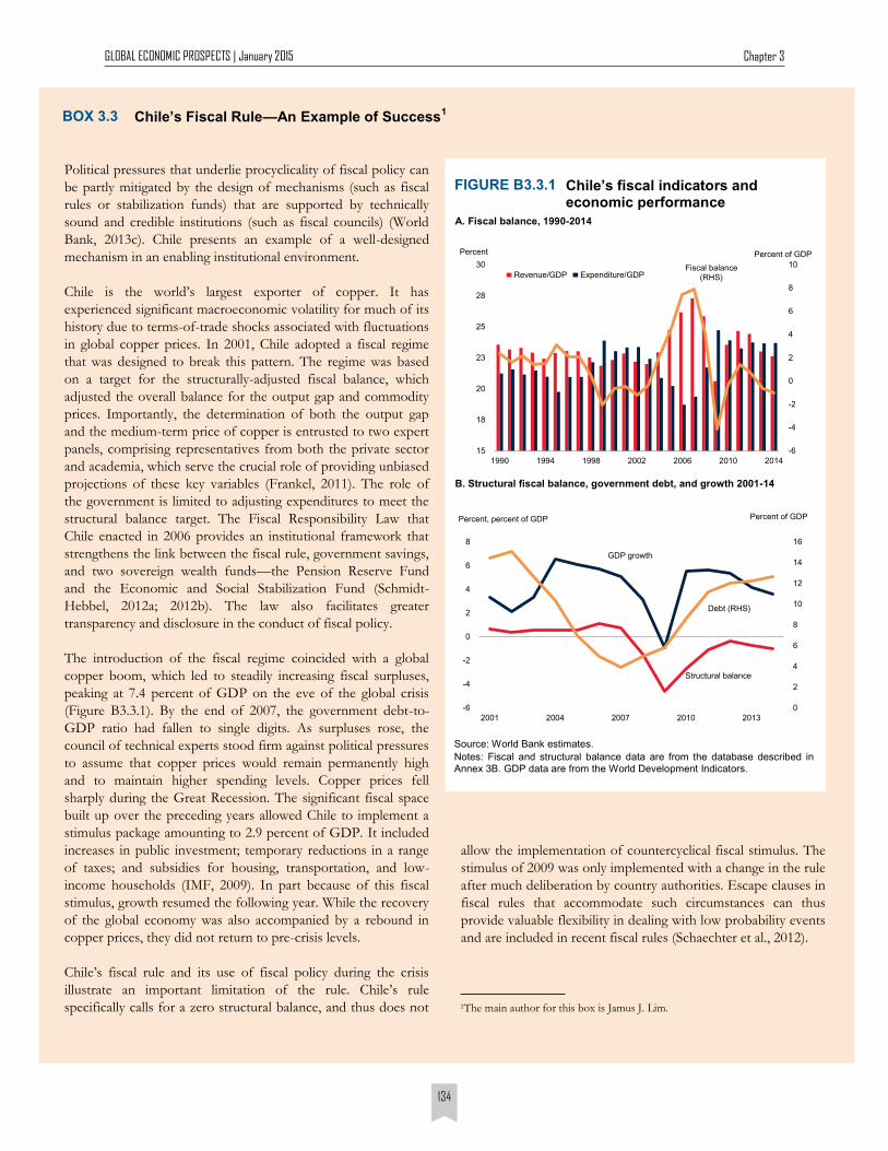
Chile’s Fiscal Rule—An Example of Success1 BOX 3.3
Political pressures that underlie procyclicality of fiscal policy can
be partly mitigated by the design of mechanisms (such as fiscal
rules or stabilization funds) that are supported by technically
sound and credible institutions (such as fiscal councils) (World
Bank, 2013c). Chile presents an example of a well-designed
mechanism in an enabling institutional environment.
Chile is the world’s largest exporter of copper. It has
experienced significant macroeconomic volatility for much of its
history due to terms-of-trade shocks associated with fluctuations
in global copper prices. In 2001, Chile adopted a fiscal regime
that was designed to break this pattern. The regime was based
on a target for the structurally-adjusted fiscal balance, which
adjusted the overall balance for the output gap and commodity
prices. Importantly, the determination of both the output gap
and the medium-term price of copper is entrusted to two expert
panels, comprising representatives from both the private sector
and academia, which serve the crucial role of providing unbiased
projections of these key variables (Frankel, 2011). The role of
the government is limited to adjusting expenditures to meet the
structural balance target. The Fiscal Responsibility Law that
Chile enacted in 2006 provides an institutional framework that
strengthens the link between the fiscal rule, government savings,
and two sovereign wealth funds—the Pension Reserve Fund
and the Economic and Social Stabilization Fund (Schmidt-
Hebbel, 2012a; 2012b). The law also facilitates greater
transparency and disclosure in the conduct of fiscal policy.
The introduction of the fiscal regime coincided with a global
copper boom, which led to steadily increasing fiscal surpluses,
peaking at 7.4 percent of GDP on the eve of the global crisis
(Figure B3.3.1). By the end of 2007, the government debt-to-
GDP ratio had fallen to single digits. As surpluses rose, the
council of technical experts stood firm against political pressures
to assume that copper prices would remain permanently high
and to maintain higher spending levels. Copper prices fell
sharply during the Great Recession. The significant fiscal space
built up over the preceding years allowed Chile to implement a
stimulus package amounting to 2.9 percent of GDP. It included
increases in public investment; temporary reductions in a range
of taxes; and subsidies for housing, transportation, and low-
income households (IMF, 2009). In part because of this fiscal
stimulus, growth resumed the following year. While the recovery
of the global economy was also accompanied by a rebound in
copper prices, they did not return to pre-crisis levels.
Chile’s fiscal rule and its use of fiscal policy during the crisis
illustrate an important limitation of the rule. Chile’s rule
specifically calls for a zero structural balance, and thus does not
allow the implementation of countercyclical fiscal stimulus. The
stimulus of 2009 was only implemented with a change in the rule
after much deliberation by country authorities. Escape clauses in
fiscal rules that accommodate such circumstances can thus
provide valuable flexibility in dealing with low probability events
and are included in recent fiscal rules (Schaechter et al., 2012).
Structural balance
GDP growth
Debt (RHS)
0
2
4
6
8
10
12
14
16
-6
-4
-2
0
2
4
6
8
2001 2004 2007 2010 2013
Percent, percent of GDP Percent of GDP
-6
-4
-2
0
2
4
6
8
10
15
18
20
23
25
28
30
1990 1994 1998 2002 2006 2010 2014
Fiscal balance (RHS)Revenue/GDP Expenditure/GDP
Percent Percent of GDP
Source: World Bank estimates.
Notes: Fiscal and structural balance data are from the database described in Annex 3B. GDP data are from the World Development Indicators.
Chile’s fiscal indicators and economic performance
FIGURE B3.3.1
A. Fiscal balance, 1990-2014
B. Structural fiscal balance, government debt, and growth 2001-14
GLOBAL ECONOMIC PROSPECTS | January 2015 Chapter 3
135
stabilization funds separate government expenditure
from fluctuations in the availability of revenues, they can
be important institutional mechanisms for improving
fiscal space, while mitigating fiscal procyclicality.
Although the empirical evidence is somewhat mixed, a
number of studies find that stabilization funds can help
improve fiscal discipline (Fasano, 2000) and expand fiscal
space (Bagattini, 2011). Stabilization funds do appear to
smooth government expenditure, reducing their volatility
by as much as 13 percent compared to economies
without such funds (Sugawara, 2014).
While a stabilization fund can be a powerful fiscal tool to
manage fiscal resources and create fiscal space, the
establishment itself does not guarantee its success. Cross-
country evidence even suggests that the effectiveness of a
particular stabilization fund in shielding the domestic
economy from commodity price volatility depends largely
on government commitment to fiscal discipline and
macroeconomic management, rather than on just the
existence of the instrument itself (Gill et al., 2014).
Proper designs and strong institutional environments that
support their operations are crucial factors for the
success of stabilization funds.
Among resource-rich economies, Norway and Chile are
often treated as examples of economies with stabilization
funds that are based on specific resource revenues and
associated with good fiscal management (Schmidt-
Hebbel, 2012a, 2012b). Norway’s Government Pension
Fund and Chile’s Economic and Social Stabilization
Fund are ranked highest and third, respectively, in a
scoring of 58 sovereign wealth funds and government
pension funds (Bagnall and Truman, 2013). The main
characteristics that distinguish Norway’s and Chile’s
funds from those with lower scores are governance and
transparency and accountability of fund operations.
Medium-Term Expenditure Frameworks (MTEF)
MTEFs were first introduced to facilitate modern public
financial management in pursuit of long-run policy
priorities in OECD economies. Among developing
economies, they gained prominence in the late 1990s, as
annual budgets were perceived to create uncertainty about
future budgetary commitments. International financial
agencies, such as the World Bank, have also sought to
encourage stable allocations toward poverty reduction
targets. More than two-thirds of all economies have
adopted MTEFs of some form (World Bank, 2013c).
The objective of MTEFs is to establish or improve
credibility in the budgetary process. They seek to ensure a
transparent budgetary process, where government
agencies establish credible contracts for the allocation of
public resources toward agreed strategic priorities, over
an average of three years. The most common design of
MTEFs translates macroeconomic objectives into budget
aggregates and detailed spending plans; less sophisticated
approaches target either aggregate fiscal goals, or micro-
level costs and outcomes.
Empirical evidence suggests that credible MTEFs can
significantly improve fiscal discipline (World Bank, 2013c).
Furthermore, the results tend to be more positive for
more sophisticated frameworks (Grigoli et al., 2012).
Significant heterogeneity exists, however, and certain
studies limited to smaller regional samples have been
unable to find conclusive evidence, possibly reflecting
shortcomings in the practical implementation of MTEFs.27
Keys to robust implementation are coordination with
broader public sector reform, and sensitivity to country
characteristics (World Bank, 2013c). For example, Jordan’s
MTEF was a component of major public financial
management reforms in 2004 and part of the national
development strategy. The MTEF’s specific objective was
to improve fiscal discipline through realistic revenue
projections, followed by better expenditure prioritization
and the identification of fiscal space. In the case of South
Africa, the MTEF was introduced in the context of high
government debt and a combination of underspending by
the central government and overspending by provincial
governments. Underspending and overspending were
both reduced following the introduction of the MTEF.
One of the lessons from the experiences of South Africa,
Tanzania, and Uganda is the need for realistic expectations
during the preparation of the budget, without which even
well-designed MTEFs cannot succeed (Holmes and
Evans, 2003).
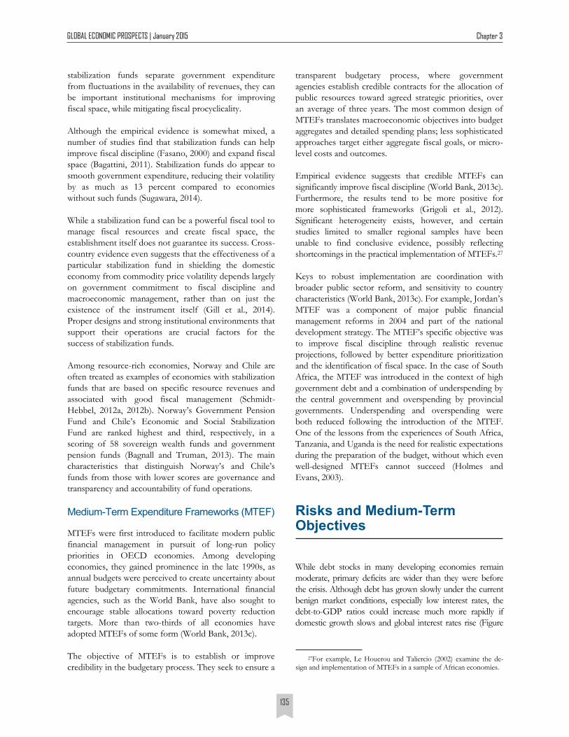
Risks and Medium-Term Objectives
While debt stocks in many developing economies remain
moderate, primary deficits are wider than they were before
the crisis. Although debt has grown slowly under the current
benign market conditions, especially low interest rates, the
debt-to-GDP ratios could increase much more rapidly if
domestic growth slows and global interest rates rise (Figure
27For example, Le Houerou and Taliercio (2002) examine the de-sign and implementation of MTEFs in a sample of African economies.
GLOBAL ECONOMIC PROSPECTS | January 2015 Chapter 3
136
Sustainability gaps under different conditions in 2013
Source: World Bank estimates.
Note: The sustainability gap is the difference between the primary balance and an estimated debt-stabilizing primary balance, which depends on as-sumptions about interest rates and growth rates. For a given country, current market conditions refer to 2013 interest and growth rates, while historic conditions refer to the sample average during 1980–2013. A negative value suggests that the balance is debt-increasing, a value of zero suggests that the balance holds debt constant, and positive values suggest that the balance is debt-reducing. A redder color indicates a more negative sustainability gap; a greener color a more positive gap. If the data was updated to 2014, some countries would show more benign sustainability gaps (e.g. Spain) while others would show lower ones.
FIGURE 3.13
In some EMEs and FMEs, fiscal risks would increase under historic market conditions.
A. Current market conditions
B. Historic market conditions
GLOBAL ECONOMIC PROSPECTS | January 2015 Chapter 3
137
3.13).28 This is especially relevant for some FMEs that have
placed sovereign bonds in international markets recently and
have increased their exposure to risks linked to global
financing conditions.29 Some economies could thus become
more vulnerable to sharp increases in borrowing cost. The
historical experience discussed earlier also highlights several
instances in recent decades when debt ratios rose sharply.
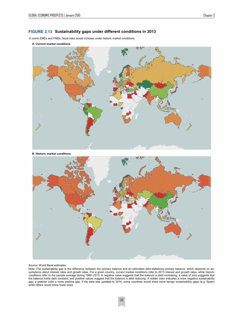
Private sector vulnerabilities are another source of risk that
EMEs and FMEs should monitor since they have been
associated with debt crises in the past (Box 3.4). Corporate
and household debt in EMEs and FMEs has risen since the
crisis (Figure 3.14). This rise has been substantial in some
EMEs, with aggregate non-financial corporate debt growing
by 39 percent over 2007–13. Moreover, in some countries,
rising private sector debt has been accompanied by
deteriorating fiscal sustainability. Some countries have
already taken measures to restrain private credit growth.30
Rapid currency depreciations can be another source of risk
in some countries, where nonfinancial firms have been
borrowing substantially in international markets in foreign
currencies, but depositing the proceeds in local currencies in
domestic financial systems (IDB, 2014). Sharp depreciations
could thus strain the solvency of domestic firms and weaken
the soundness of domestic financial sectors.
The recent slump in oil prices presents both risks and
opportunities for developing countries. For oil exporters,
the slump could result in loss of oil revenues, eroding
their fiscal space. At the same time, many countries have
substantial food and fuel subsidies. Continued soft
commodity prices (as projected for 2015-16) would offer
an opportunity to implement subsidy reform which
would both help rebuild fiscal space and lessen
distortions associated with these subsidies.
Over the medium term, in view of these risks as well as the
desirability of strengthening fiscal space, developing
economies will need to return their fiscal positions to more
sustainable levels. The appropriate speed of adjustment,
however, depends on a host of country-specific factors,
including the cyclical position of the economy and
constraints on monetary policy. If monetary policy
normalization in advanced economies results in higher
interest rates, a sharp drop in or reversal of capital flows
could constrain monetary policy responses to weakening
growth. Fiscal space would help ensure that fiscal policy
remains available as a countercyclical policy tool. A wider
fiscal space would not only increase the likelihood that fiscal
stimulus is a feasibly policy option, but would also improve
its effectiveness. This implies that adhering to an appropriate
medium-term program of deficit reduction offers the
prospect of a much more effective fiscal policy when it is
needed most. For instance, the estimates from the baseline
model suggest that fiscal multipliers would be reduced by
one-third from pre-crisis levels (Figure 3.15).
28The relationship between primary balances and debt is character-ized by the sustainability gap. The sustainability gap measure here is based on long rates, and as such does not take into account the fact that developing economies also hold short term debt. However, to the extent that the average maturity of bond issuances in developing economies is lengthening (Chapter 1), the bias from using the long rates is likely small.
29See Chapter 1 for discussion on Cote d’Ivoire and Kenya, and IMF (2104d) for the cases of Ghana and Zambia.
30World Bank (2014b) describes recent efforts to reduce vulnerabili-ties in China, Malaysia, Thailand, and Vietnam.
Private sector vulnerabilities FIGURE 3.14
Credit to the private sector has expanded since 2007 in EMEs and FMEs. In some countries this expansion has been rapid and also associated with fiscal sustainability challenges.
Source: World Bank estimates.
Note: Panel A shows domestic private sector credit as percent of GDP in EMEs and FMEs. In Panel B, the size of the circle is proportional to domestic private credit-to–GDP ratio. The sustainability gap is the difference between the primary balance and an estimated debt-stabilizing primary balance based on interest rates and growth rates in 2013. A negative value suggests that the balance is debt increasing, a value of zero suggests that the balance holds debt constant, and positive values suggest that the balance is debt reducing. All economies in the figure are EMEs and FMEs with domestic private credit-to-GDP ratios greater than 50 percent. Sustainability gap data are from the database described in Annex 3B; private-sector credit data from World Development Indicators.
A. Private sector credit evolution
0
10
20
30
40
50
60
70
EME FME
2007 2013Percent
B. Credit growth and sustainability gaps in 2013
BGRIND
POL
COLCZE
BRA
RUSUKR
HRV
VNM
LBN
CHL
MYS CHN
THAZAF
-2
0
2
4
6
8
10
12
14
-5 -4 -3 -2 -1 0 1 2 3
Sustainability gap (2013)
Change in private sector credit to GDP ratio2012-13 (%)
GLOBAL ECONOMIC PROSPECTS | January 2015 Chapter 3
138
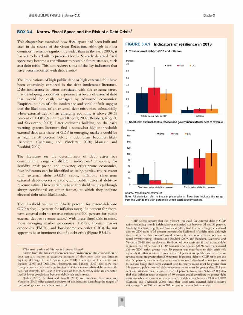
Narrow Fiscal Space and the Risk of a Debt Crisis1 BOX 3.4
This chapter has examined how fiscal space had been built and
used in the course of the Great Recession. Although in most
countries it remains significantly wider than in the early 2000s, it
has yet to be rebuilt to pre-crisis levels. Severely depleted fiscal
space may become a contributor to possible future stresses, such
as a debt crisis. This box reviews some of the key indicators that
have been associated with debt crises.2
The implications of high public debt or high external debt have
been extensively explored in the debt intolerance literature.
Debt intolerance is often associated with the extreme stress
that developing economies experience at levels of external debt
that would be easily managed by advanced economies.
Empirical studies of debt intolerance and serial default suggest
that the likelihood of an external debt crisis rises substantially
when external debt of an emerging economy is above 30-35
percent of GDP (Reinhart and Rogoff, 2009; Reinhart, Rogoff,
and Savastano, 2003). Later estimates building on the early
warning systems literature find a somewhat higher threshold:
external debt as a share of GDP in emerging markets could be
as high as 50 percent before a debt crisis becomes likely
(Bandiera, Cuaresma, and Vinclette., 2010; Manasse and
Roubini, 2009).
The literature on the determinants of debt crises has
considered a range of different indicators.3 However, for
liquidity crisis-prone and solvency crisis-prone economies,
four indicators can be identified as being particularly relevant:
total external debt-to-GDP ratios, inflation, short-term
external debt-to-reserve ratios, and public external debt-to-
revenue ratios. These variables have threshold values (although
always conditional on other factors) at which they indicate
elevated debt crisis likelihoods.
The threshold values are 31–50 percent for external-debt-to
GDP ratios; 11 percent for inflation rates; 134 percent for short-
term external debt-to reserve ratios; and 300 percent for public
external debt-to-revenue ratios.4 With these thresholds in mind,
most emerging market economies (EMEs), frontier market
economies (FMEs), and low-income countries (LICs) do not
appear to be at imminent risk of a debt crisis (Figure B3.4.1).
Source: World Bank estimates.
Note: All statistics refer to the sample medians. Error bars indicate the range from the 25th to the 75th percentile within each country sample.
Indicators of resilience in 2013 FIGURE 3.4.1
A. Total external debt-to-GDP and inflation
B. Short-term external debt to reserve and government external debt to revenue
0
10
20
30
40
50
60
70
Total external debt to GDP Inflation
EME FME LIC
Percent
0
20
40
60
80
100
120
140
160
Short term external debt to reserve Public external debt to revenue
EME FME LIC
Percent
-
1This main author of this box is S. Amer Ahmed. 2Aside from the broader macroeconomic environment, the composition of
debt can also matter, as excessive amounts of short-term debt can threaten liquidity (Detragiache and Spilimbergo, 2004). Eichengreen, Hausmann, and Panizza (2009) and Dell’Erba, Hausmann, and Panizza (2013) also show that foreign currency debt and large foreign liabilities can exacerbate debt vulnerabili-ties. For example, EMEs with low levels of foreign currency debt are character-ized by lower correlations between debt levels and spreads.
3Jedidi (2013), Reinhart and Rogoff (2011) and Bandiera, Cuaresma, and Vinclette (2010) offer extensive reviews of the literature, describing the ranges of methodologies and variables considered.
4IMF (2002) reports that the relevant threshold for external debt-to-GDP ratios (excluding heavily indebted poor countries) was between 31 and 39 percent. Similarly, Reinhart, Rogoff, and Savastano (2003) find that, on average, an external debt-to-GDP ratio of 35 percent increases the likelihood of a debt crisis, although they caution that this threshold could be lower if the economy has a poor institu-tional investor rating. Manasse and Roubini (2009) and Bandiera, Cuaresma, and Vinclette (2010) find an elevated likelihood of debt crisis risk if total external debt is greater than 50 percent of GDP. Manasse and Roubini (2009) note that external debt-to-GDP ratios greater than 50 percent can contribute to debt crisis risk especially if inflation rates are greater than 11 percent and public external debt-to-revenue ratios are greater than 300 percent. If external-debt-to-GDP ratios are less than 50 percent, then other key indicators must reach threshold values for a crisis to become likely: short-term external debt-to-reserve ratios must be greater than 134 percent, public external debt-to-revenue ratios must be greater than 215 per-cent and inflation must be greater than 11 percent. Kraay and Nehru (2006) also find that inflation rates in excess of 40 percent could contribute to greater debt crisis risk while a cross-country event study of debt crises between 1980 and 2002 (Ciarlone and Trebeschi, 2006) finds that short-term external debt-to-reserve ratios surge from 220 percent to 383 percent in the year before a crisis.
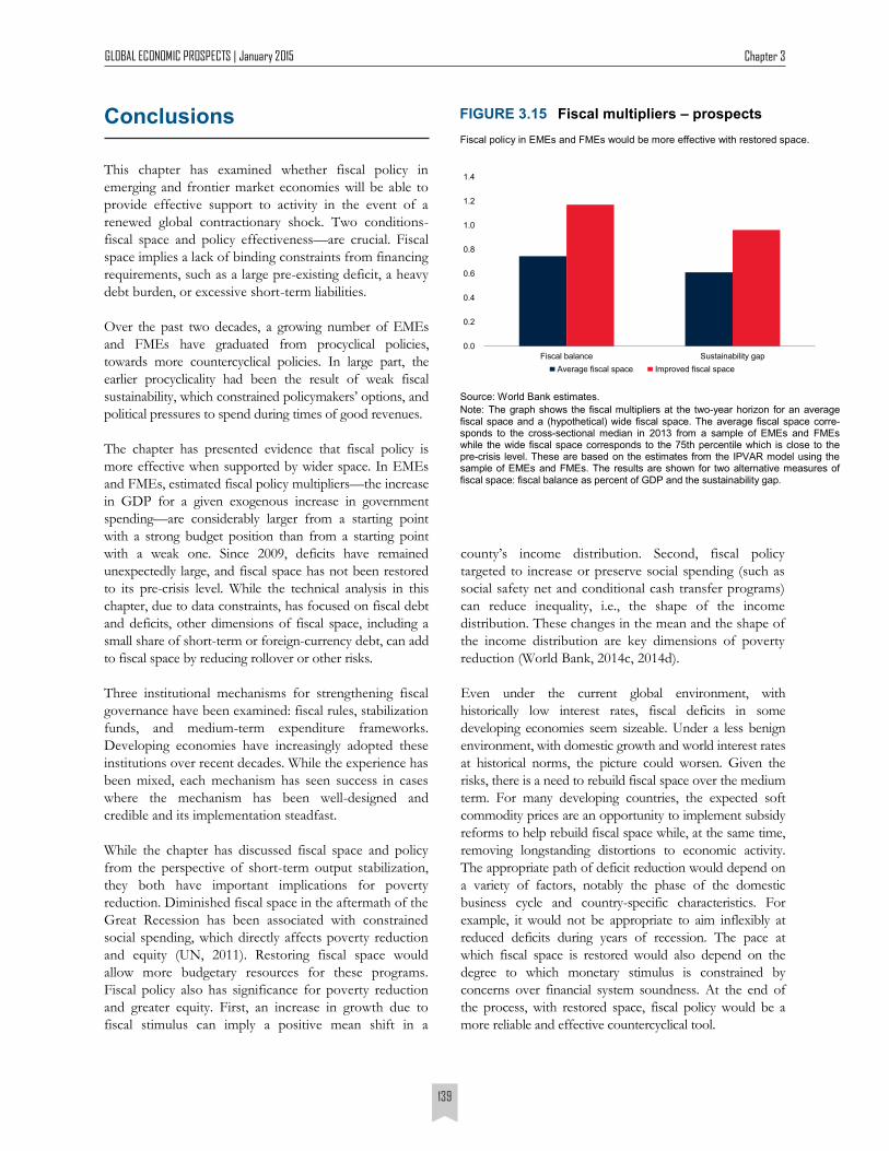
GLOBAL ECONOMIC PROSPECTS | January 2015 Chapter 3
139
Conclusions
This chapter has examined whether fiscal policy in
emerging and frontier market economies will be able to
provide effective support to activity in the event of a
renewed global contractionary shock. Two conditions-
fiscal space and policy effectiveness—are crucial. Fiscal
space implies a lack of binding constraints from financing
requirements, such as a large pre-existing deficit, a heavy
debt burden, or excessive short-term liabilities.
Over the past two decades, a growing number of EMEs
and FMEs have graduated from procyclical policies,
towards more countercyclical policies. In large part, the
earlier procyclicality had been the result of weak fiscal
sustainability, which constrained policymakers’ options, and
political pressures to spend during times of good revenues.
The chapter has presented evidence that fiscal policy is
more effective when supported by wider space. In EMEs
and FMEs, estimated fiscal policy multipliers—the increase
in GDP for a given exogenous increase in government
spending—are considerably larger from a starting point
with a strong budget position than from a starting point
with a weak one. Since 2009, deficits have remained
unexpectedly large, and fiscal space has not been restored
to its pre-crisis level. While the technical analysis in this
chapter, due to data constraints, has focused on fiscal debt
and deficits, other dimensions of fiscal space, including a
small share of short-term or foreign-currency debt, can add
to fiscal space by reducing rollover or other risks.
Three institutional mechanisms for strengthening fiscal
governance have been examined: fiscal rules, stabilization
funds, and medium-term expenditure frameworks.
Developing economies have increasingly adopted these
institutions over recent decades. While the experience has
been mixed, each mechanism has seen success in cases
where the mechanism has been well-designed and
credible and its implementation steadfast.
While the chapter has discussed fiscal space and policy
from the perspective of short-term output stabilization,
they both have important implications for poverty
reduction. Diminished fiscal space in the aftermath of the
Great Recession has been associated with constrained
social spending, which directly affects poverty reduction
and equity (UN, 2011). Restoring fiscal space would
allow more budgetary resources for these programs.
Fiscal policy also has significance for poverty reduction
and greater equity. First, an increase in growth due to
fiscal stimulus can imply a positive mean shift in a
county’s income distribution. Second, fiscal policy
targeted to increase or preserve social spending (such as
social safety net and conditional cash transfer programs)
can reduce inequality, i.e., the shape of the income
distribution. These changes in the mean and the shape of
the income distribution are key dimensions of poverty
reduction (World Bank, 2014c, 2014d).
Even under the current global environment, with
historically low interest rates, fiscal deficits in some
developing economies seem sizeable. Under a less benign
environment, with domestic growth and world interest rates
at historical norms, the picture could worsen. Given the
risks, there is a need to rebuild fiscal space over the medium
term. For many developing countries, the expected soft
commodity prices are an opportunity to implement subsidy
reforms to help rebuild fiscal space while, at the same time,
removing longstanding distortions to economic activity.
The appropriate path of deficit reduction would depend on
a variety of factors, notably the phase of the domestic
business cycle and country-specific characteristics. For
example, it would not be appropriate to aim inflexibly at
reduced deficits during years of recession. The pace at
which fiscal space is restored would also depend on the
degree to which monetary stimulus is constrained by
concerns over financial system soundness. At the end of
the process, with restored space, fiscal policy would be a
more reliable and effective countercyclical tool.
Fiscal multipliers – prospects FIGURE 3.15
Fiscal policy in EMEs and FMEs would be more effective with restored space.
Source: World Bank estimates.
Note: The graph shows the fiscal multipliers at the two-year horizon for an average fiscal space and a (hypothetical) wide fiscal space. The average fiscal space corre-sponds to the cross-sectional median in 2013 from a sample of EMEs and FMEs while the wide fiscal space corresponds to the 75th percentile which is close to the pre-crisis level. These are based on the estimates from the IPVAR model using the sample of EMEs and FMEs. The results are shown for two alternative measures of fiscal space: fiscal balance as percent of GDP and the sustainability gap.
0.0
0.2
0.4
0.6
0.8
1.0
1.2
1.4
Fiscal balance Sustainability gap
Average fiscal space Improved fiscal space
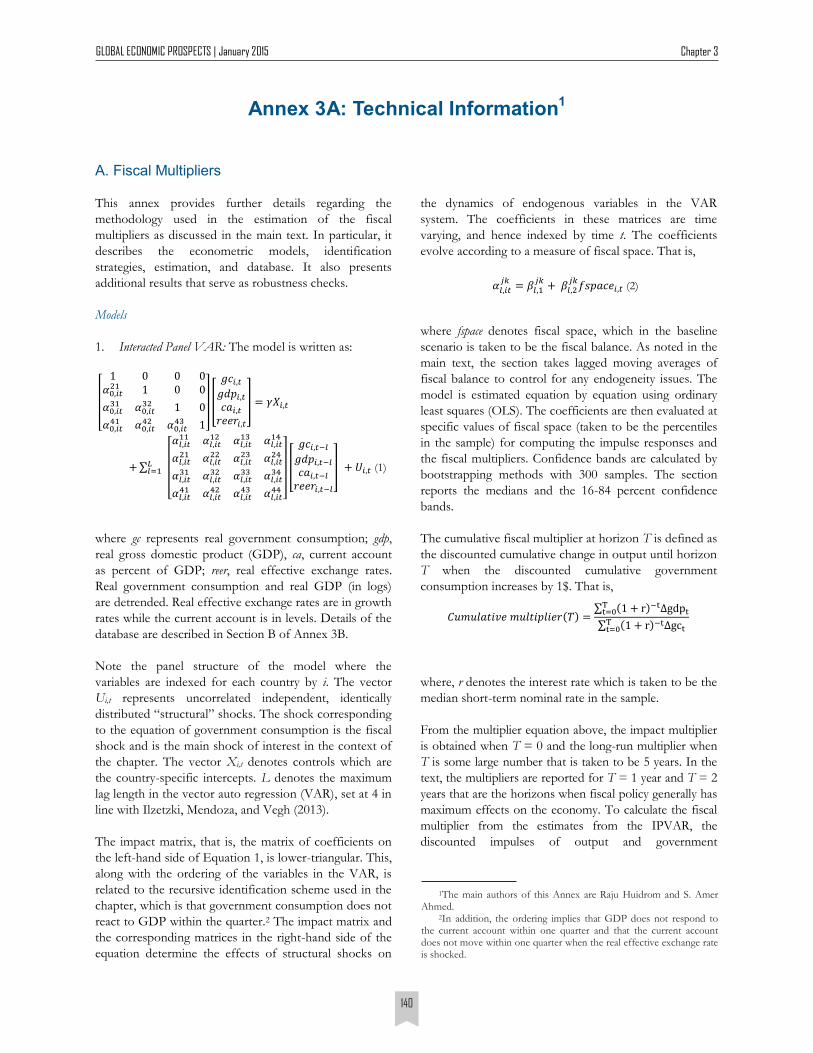
GLOBAL ECONOMIC PROSPECTS | January 2015 Chapter 3
140
A. Fiscal Multipliers
This annex provides further details regarding the
methodology used in the estimation of the fiscal
multipliers as discussed in the main text. In particular, it
describes the econometric models, identification
strategies, estimation, and database. It also presents
additional results that serve as robustness checks.
Models
1. Interacted Panel VAR: The model is written as:
where gc represents real government consumption; gdp,
real gross domestic product (GDP), ca, current account
as percent of GDP; reer, real effective exchange rates.
Real government consumption and real GDP (in logs)
are detrended. Real effective exchange rates are in growth
rates while the current account is in levels. Details of the
database are described in Section B of Annex 3B.
Note the panel structure of the model where the
variables are indexed for each country by i. The vector
Ui,t represents uncorrelated independent, identically
distributed “structural” shocks. The shock corresponding
to the equation of government consumption is the fiscal
shock and is the main shock of interest in the context of
the chapter. The vector Xi,t denotes controls which are
the country-specific intercepts. L denotes the maximum
lag length in the vector auto regression (VAR), set at 4 in
line with Ilzetzki, Mendoza, and Vegh (2013).
The impact matrix, that is, the matrix of coefficients on
the left-hand side of Equation 1, is lower-triangular. This,
along with the ordering of the variables in the VAR, is
related to the recursive identification scheme used in the
chapter, which is that government consumption does not
react to GDP within the quarter.2 The impact matrix and
the corresponding matrices in the right-hand side of the
equation determine the effects of structural shocks on
the dynamics of endogenous variables in the VAR
system. The coefficients in these matrices are time
varying, and hence indexed by time t. The coefficients
evolve according to a measure of fiscal space. That is,
where fspace denotes fiscal space, which in the baseline
scenario is taken to be the fiscal balance. As noted in the
main text, the section takes lagged moving averages of
fiscal balance to control for any endogeneity issues. The
model is estimated equation by equation using ordinary
least squares (OLS). The coefficients are then evaluated at
specific values of fiscal space (taken to be the percentiles
in the sample) for computing the impulse responses and
the fiscal multipliers. Confidence bands are calculated by
bootstrapping methods with 300 samples. The section
reports the medians and the 16-84 percent confidence
bands.
The cumulative fiscal multiplier at horizon T is defined as
the discounted cumulative change in output until horizon
T when the discounted cumulative government
consumption increases by 1$. That is,
where, r denotes the interest rate which is taken to be the
median short-term nominal rate in the sample.
From the multiplier equation above, the impact multiplier
is obtained when T = 0 and the long-run multiplier when
T is some large number that is taken to be 5 years. In the
text, the multipliers are reported for T = 1 year and T = 2
years that are the horizons when fiscal policy generally has
maximum effects on the economy. To calculate the fiscal
multiplier from the estimates from the IPVAR, the
discounted impulses of output and government
Annex 3A: Technical Information1
(2)
1The main authors of this Annex are Raju Huidrom and S. Amer Ahmed.
2In addition, the ordering implies that GDP does not respond to the current account within one quarter and that the current account does not move within one quarter when the real effective exchange rate is shocked.
(1)
GLOBAL ECONOMIC PROSPECTS | January 2015 Chapter 3
141
3The forecast error series is only available at the semi-annual fre-quency and accordingly, the model is estimated only at that frequency. The series is available for only 29 countries (22 AMEs and 7 EMEs and FMEs) and during the period 1987-2013. See Section B of the Annex 3B for the details of this database.
consumption are cumulated at different horizons. Then,
the ratio of the two impulses is scaled by the average
government consumption to GDP ratio.
2. Panel SVAR: The model is written as:
where the notations closely follow the IPVAR. The
vector C0 captures the intercept terms. The set of
variables included in the VAR is also the same as before,
and so is the identification scheme. Thus, the impact
matrix retains the lower triangular structure. Unlike the
IPVAR, the law of motion of the coefficients in
Equation (2) is absent in this model. Accordingly, the
VAR coefficients are no longer indexed by country i and
time t. In other words, the panel SVAR (structural vector
auto regression) only estimates a single set of coefficients
from the pooled sample. The sample is split by episodes
of wide and narrow fiscal space at an exogenous cut-off
point, determined by judgment, to calculate estimates
that vary by fiscal space. The IPVAR, on the other hand,
estimates fiscal multipliers for continuous levels of fiscal
space, thereby avoiding the cut-off choice. The
confidence bands are based on 1000 Monte Carlo draws.
Country fixed effects are taken into account by removing
means and trends country by country. As in the IPVAR,
a maximum lag length of 4 is used.
The model is also used to infer the evolution of the
cyclicality of fiscal policy in developing economies. To
that end, the model is estimated during three sub-samples
(1980–1999, 2000–2007, and 2008–2014) and the
response of government consumption to GDP shocks is
calculated for each sub-sample. Fiscal policy is procyclical
when that response is positive and statistically significant.
3. Local Projections Model: The model is written as:
where x indicates fiscal space normalized to have zero mean
and unit variance. Like the previous models, fiscal space is
measured by lagged moving averages of fiscal balances as
percent of GDP. The parameter γ is calibrated as 2.5. ΔYi,t+h
denotes the growth rate of output of country i at horizon h,
FEG is the forecast error of government consumption. The
parameter captures country fixed effects and the time trend.
The indicator function I pins down the probability that the
economy is in a regime of narrow fiscal space.
The local projections model is a single equation model
unlike the multivariate framework of the IPVAR and the
panel SVAR. In this model, fiscal shocks are defined as
fiscal surprises constructed outside the model as the
forecast errors of government consumption. The forecast
errors proxy unanticipated fiscal shocks in that they
represent any surprises in government consumption over
and above what private agents expect them to be given
their available information set. The forecast errors of
government consumption (in growth rates) are compiled
from various OECD publications.3
The effects of fiscal policy on output are then traced out
by regressing output on the fiscal surprises, taking into
account country fixed effects. Those effects are
dependent on whether the economy is in a regime of
wide or narrow fiscal space, as pinned down by the
indicator function. Lags of government consumption and
GDP are included as controls to purge any effects that
they may have had on the forecasts of government
consumption. The model is separately estimated for each
horizon, which is then used to project the dynamic effects
of fiscal shocks on output.
Additional results
This section presents additional results that serve as
robustness checks.
Fiscal multipliers during recessions and expansions:
Annex 3A.1 shows that fiscal multipliers are larger
during periods of recessions than expansions – a
result consistent with standard macroeconomic
with
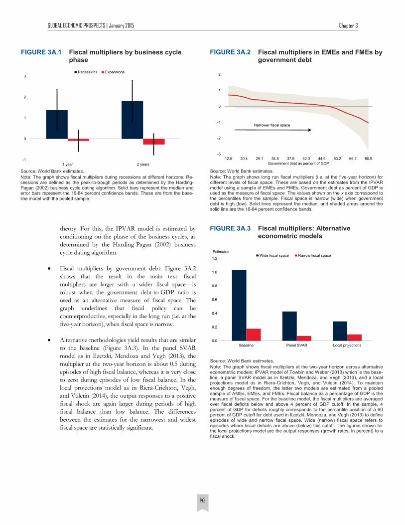
GLOBAL ECONOMIC PROSPECTS | January 2015 Chapter 3
142
theory. For this, the IPVAR model is estimated by
conditioning on the phase of the business cycles, as
determined by the Harding-Pagan (2002) business
cycle dating algorithm.
Fiscal multipliers by government debt: Figure 3A.2
shows that the result in the main text—fiscal
multipliers are larger with a wider fiscal space—is
robust when the government debt-to-GDP ratio is
used as an alternative measure of fiscal space. The
graph underlines that fiscal policy can be
counterproductive, especially in the long run (i.e. at the
five-year horizon), when fiscal space is narrow.
Alternative methodologies yield results that are similar
to the baseline (Figure 3A.3). In the panel SVAR
model as in Ilzetzki, Mendoza and Vegh (2013), the
multiplier at the two-year horizon is about 0.5 during
episodes of high fiscal balance, whereas it is very close
to zero during episodes of low fiscal balance. In the
local projections model as in Riera-Crichton, Vegh,
and Vuletin (2014), the output responses to a positive
fiscal shock are again larger during periods of high
fiscal balance than low balance. The differences
between the estimates for the narrowest and widest
fiscal space are statistically significant.
Fiscal multipliers in EMEs and FMEs by government debt
FIGURE 3A.2
Source: World Bank estimates.
Note: The graph shows long run fiscal multipliers (i.e. at the five-year horizon) for different levels of fiscal space. These are based on the estimates from the IPVAR model using a sample of EMEs and FMEs. Government debt as percent of GDP is used as the measure of fiscal space. The values shown on the x axis correspond to the percentiles from the sample. Fiscal space is narrow (wide) when government debt is high (low). Solid lines represent the median, and shaded areas around the solid line are the 16-84 percent confidence bands.
-3
-2
-1
0
1
2
12.5 20.4 29.1 34.5 37.9 42.0 44.9 53.2 66.2 80.9
Government debt as percent of GDP
Narrower fiscal space
Fiscal multipliers by business cycle phase
FIGURE 3A.1
Source: World Bank estimates.
Note: The graph shows fiscal multipliers during recessions at different horizons. Re-cessions are defined as the peak-to-trough periods as determined by the Harding-Pagan (2002) business cycle dating algorithm. Solid bars represent the median and error bars represent the 16-84 percent confidence bands. These are from the base-line model with the pooled sample.
-1
0
1
2
3
1 year 2 years
Recessions Expansions
0.0
0.2
0.4
0.6
0.8
1.0
1.2
Baseline Panel SVAR Local projections
Wide fiscal space Narrow fiscal spaceEstimates
Fiscal multipliers: Alternative econometric models
FIGURE 3A.3
Source: World Bank estimates.
Note: The graph shows fiscal multipliers at the two-year horizon across alternative econometric models: IPVAR model of Towbin and Weber (2013) which is the base-line, a panel SVAR model as in Ilzetzki, Mendoza, and Vegh (2013), and a local projections model as in Riera-Crichton, Vegh, and Vuletin (2014). To maintain enough degrees of freedom, the latter two models are estimated from a pooled sample of AMEs, EMEs, and FMEs. Fiscal balance as a percentage of GDP is the measure of fiscal space. For the baseline model, the fiscal multipliers are averaged over fiscal deficits below and above 4 percent of GDP cutoff. In the sample, 4 percent of GDP for deficits roughly corresponds to the percentile position of a 60 percent of GDP cutoff for debt used in Ilzetzki, Mendoza, and Vegh (2013) to define episodes of wide and narrow fiscal space. Wide (narrow) fiscal space refers to episodes where fiscal deficits are above (below) this cutoff. The figures shown for the local projections model are the output responses (growth rates, in percent) to a fiscal shock.
GLOBAL ECONOMIC PROSPECTS | January 2015 Chapter 3
143
B. Identifying Contraction Events
This chapter uses an event study to examine how fiscal
space and fiscal policy in EMEs and FMEs changes in
the runup to, during, and immediately after a contraction
episode. Three sets of comparisons are made. The first
set is between EMEs and FMEs in a particular
contraction episode to highlight their differences within
the same episode. The second set is between economies
with differing levels of fiscal space within the same
contraction episode. The third set is between economies’
contraction episodes during the Great Recession and
during pre-2008 contraction episodes.
A country is considered here to have experienced a
contraction event if its growth in a given year fulfills two
conditions. The first is that the growth is negative (i.e., a
contraction), and the second is that the growth is more
than one standard deviation below the average that the
country experienced in the 1990–2013 period. The year
of the event, as defined, is then ‘t=0.’ If there are two or
more contractionary episodes within a five-year period,
the year with the greatest growth contraction is taken as
‘t=0.’ This is a variation of the censoring rule applied by
IMF (2012a) in its application of the Harding and Pagan
(2002) quarterly business cycle dating methodology to
annual data. If key fiscal space data, such as gross
government debt, are not available in the database for the
country in the event year, then the event is dropped.4
This approach identifies 101 contraction events, 50 in the
pre-2008 period and 51 in 2008–09 for the full sample of
all countries including AMEs, EMEs, and FMEs. These
events, along with their associated real GDP contraction
can be seen in Annex Tables 3A.1 and 3A.2 for EMEs
and FMEs. Episodes identified as crises but not included
in the event study because of data constraints are noted
in Annex Table 3A.3.
This definition of events considers output contractions
only. The comprehensive financial crisis database of
Laeven and Valencia (2013) has been considered a source
for event dates. However, it focuses on financial crises,
and thereby excludes episodes in many economies, such
as those in Sub-Saharan Africa. Also, some of the
episodes it considers do not necessarily have output
contractions associated with them.
4To ensure that the crisis of 1995 in Mexico is included, the data-base is augmented the IMF’s Global Data Source.
Contraction events between
1990 and 2007 TABLE 3A.1
Note: EME: Emerging Market Economy.
C ount ry Y ear C o unt ry Group R eal GD P Growt h ( %)
Argentina 2002 EM E -10.9
Bahrain 1994 EM E -0.3
Chile 1999 EM E -0.8
Côte d'Ivoire 2000 FM E -3.7
Colombia 1999 EM E -4.2
Korea, Rep. 1998 EM E -5.7
Sri Lanka 2001 EM E -1.5
M orocco 1993 EM E -1.0
M alaysia 1998 EM E -7.4
Oman 1999 EM E -0.1
Philippines 1998 EM E -0.6
M exico 1995 EM E -5.8
Contraction events in 2008
and 2009 TABLE 3A.2
Note: EME: Emerging Market Economy; FME: Frontier Market Economy.
C ount ry Y ear C o unt ry Group R eal GD P Growt h ( %)
Bulgaria 2009 FM E -5.5
Botswana 2009 FM E -7.8
Chile 2009 EM E -1.0
Cyprus 2009 FM E -1.7
Czech Republic 2009 EM E -4.5
Estonia 2009 FM E -14.1
Honduras 2009 FM E -2.4
Hungary 2009 EM E -6.8
Latvia 2009 FM E -18.0
M exico 2009 EM E -4.7
M alaysia 2009 EM E -1.5
Romania 2009 FM E -6.8
Russian Federat ion 2009 EM E -7.8
Slovak Republic 2009 EM E -4.9
Slovenia 2009 FM E -8.0
Thailand 2009 EM E -2.3
Trinidad and Tobago 2009 FM E -4.4
Turkey 2009 EM E -4.8
Ukraine 2009 FM E -14.8
South Africa 2009 EM E -1.5
Zimbabwe 2008 EM E -17.7
GLOBAL ECONOMIC PROSPECTS | January 2015 Chapter 3
144
Contraction events between 1990 and 2007 excluded because of data constraints
TABLE 3A.3
Note: EME = emerging market economy; FME = frontier market economy.
C ount ry Y ear C ount ry Group R eal GD P Growt h ( %)
Bulgaria 1992 FM E -7.3
Bulgaria 1996 FM E -9.0
Brazil 1990 EM E -4.3
Czech Republic 1991 EM E -11.6
Ecuador 1999 FM E -4.7
Estonia 1994 FM E -1.6
Honduras 1994 FM E -1.3
Honduras 1999 FM E -1.9
Hungary 1992 EM E -3.1
Indonesia 1998 EM E -13.1
Israel 2002 EM E -0.6
Kenya 1992 FM E -0.8
Latvia 1992 FM E -32.1
M acedonia, FYR 1993 FM E -7.5
M acedonia, FYR 2001 FM E -4.5
M ongolia 1993 FM E -3.2
M ongolia 2009 FM E -1.3
Peru 1990 EM E -5.1
Philippines 1991 EM E -0.6
Poland 1991 EM E -7.0
Romania 1992 FM E -8.8
Romania 1998 FM E -4.8
Russian Federat ion 1994 EM E -12.6
Rwanda 1994 FM E -50.2
Senegal 1990 FM E -0.7
Senegal 1994 FM E 0.0
Serbia 1993 FM E -30.5
Serbia 1999 FM E -11.2
Slovak Republic 1993 EM E -3.7
Slovenia 1992 FM E -5.5
Thailand 1998 EM E -10.5
Turkey 1994 EM E -4.7
Turkey 2001 EM E -5.7
Venezuela, RB 2003 EM E -7.8
South Africa 1992 EM E -2.1
Zambia 1992 FM E -1.7
Zambia 1998 FM E -1.9
Zimbabwe 1992 EM E -9.0
Zimbabwe 2003 EM E -17.0
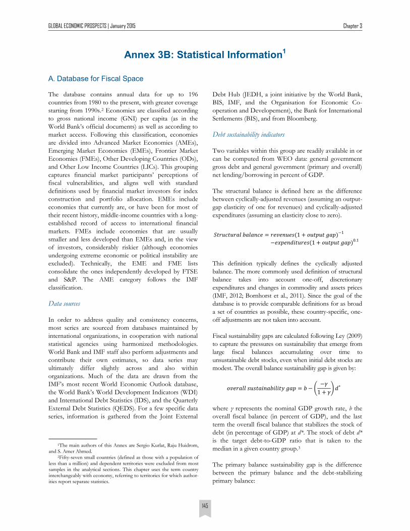
GLOBAL ECONOMIC PROSPECTS | January 2015 Chapter 3
145
A. Database for Fiscal Space
The database contains annual data for up to 196
countries from 1980 to the present, with greater coverage
starting from 1990s.2 Economies are classified according
to gross national income (GNI) per capita (as in the
World Bank’s official documents) as well as according to
market access. Following this classification, economies
are divided into Advanced Market Economies (AMEs),
Emerging Market Economies (EMEs), Frontier Market
Economies (FMEs), Other Developing Countries (ODs),
and Other Low Income Countries (LICs). This grouping
captures financial market participants’ perceptions of
fiscal vulnerabilities, and aligns well with standard
definitions used by financial market investors for index
construction and portfolio allocation. EMEs include
economies that currently are, or have been for most of
their recent history, middle-income countries with a long-
established record of access to international financial
markets. FMEs include economies that are usually
smaller and less developed than EMEs and, in the view
of investors, considerably riskier (although economies
undergoing extreme economic or political instability are
excluded). Technically, the EME and FME lists
consolidate the ones independently developed by FTSE
and S&P. The AME category follows the IMF
classification.
Data sources
In order to address quality and consistency concerns,
most series are sourced from databases maintained by
international organizations, in cooperation with national
statistical agencies using harmonized methodologies.
World Bank and IMF staff also perform adjustments and
contribute their own estimates, so data series may
ultimately differ slightly across and also within
organizations. Much of the data are drawn from the
IMF’s most recent World Economic Outlook database,
the World Bank’s World Development Indicators (WDI)
and International Debt Statistics (IDS), and the Quarterly
External Debt Statistics (QEDS). For a few specific data
series, information is gathered from the Joint External
Debt Hub (JEDH, a joint initiative by the World Bank,
BIS, IMF, and the Organisation for Economic Co-
operation and Developement), the Bank for International
Settlements (BIS), and from Bloomberg.
Debt sustainability indicators
Two variables within this group are readily available in or
can be computed from WEO data: general government
gross debt and general government (primary and overall)
net lending/borrowing in percent of GDP.
The structural balance is defined here as the difference
between cyclically-adjusted revenues (assuming an output-
gap elasticity of one for revenues) and cyclically-adjusted
expenditures (assuming an elasticity close to zero).
This definition typically defines the cyclically adjusted
balance. The more commonly used definition of structural
balance takes into account one-off, discretionary
expenditures and changes in commodity and assets prices
(IMF, 2012; Bornhorst et al., 2011). Since the goal of the
database is to provide comparable definitions for as broad
a set of countries as possible, these country-specific, one-
off adjustments are not taken into account.
Fiscal sustainability gaps are calculated following Ley (2009)
to capture the pressures on sustainability that emerge from
large fiscal balances accumulating over time to
unsustainable debt stocks, even when initial debt stocks are
modest. The overall balance sustainability gap is given by:
where γ represents the nominal GDP growth rate, b the
overall fiscal balance (in percent of GDP), and the last
term the overall fiscal balance that stabilizes the stock of
debt (in percentage of GDP) at d*. The stock of debt d*
is the target debt-to-GDP ratio that is taken to the
median in a given country group.3
The primary balance sustainability gap is the difference
between the primary balance and the debt-stabilizing
primary balance:
Annex 3B: Statistical Information1
1The main authors of this Annex are Sergio Kurlat, Raju Huidrom, and S. Amer Ahmed.
2Fifty-seven small countries (defined as those with a population of less than a million) and dependent territories were excluded from most samples in the analytical sections. This chapter uses the term country interchangeably with economy, referring to territories for which author-ities report separate statistics.
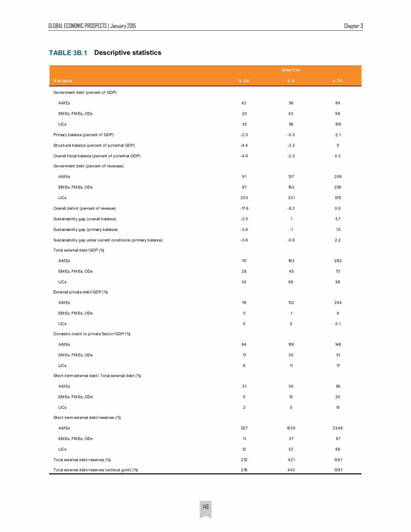
GLOBAL ECONOMIC PROSPECTS | January 2015 Chapter 3
146
Descriptive statistics TABLE 3B.1
V ariab le 0 .2 5 0 .5 0 .75
Government debt (percent of GDP)
AM Es 42 59 84
EM Es, FM Es, ODs 25 43 68
LICs 35 56 106
Primary balance (percent of GDP) -2.5 -0.3 2.1
Structural balance (percent of potent ial GDP) -4.4 -2.2 0
Overall f iscal balance (percent of potent ial GDP) -4.6 -2.3 0.2
Government debt (percent of revenues)
AM Es 91 137 208
EM Es, FM Es, ODs 87 163 259
LICs 203 331 575
Overall def icit (percent of revenue) -17.8 -8.2 0.6
Sustainability gap (overall balance) -3.5 1 5.7
Sustainability gap (primary balance) -3.6 -1 1.5
Sustainability gap under current condit ions (primary balance) -3.6 -0.6 2.2
Total external debt/GDP (%)
AM Es 117 183 282
EM Es, FM Es, ODs 28 45 73
LICs 34 66 98
External private debt/GDP (%)
AM Es 76 132 244
EM Es, FM Es, ODs 0 1 6
LICs 0 0 0.1
Domestic credit to private Sector/GDP (%)
AM Es 84 106 148
EM Es, FM Es, ODs 17 30 51
LICs 6 11 17
Short-term external debt/ Total external debt (%)
AM Es 31 39 58
EM Es, FM Es, ODs 5 12 20
LICs 2 5 10
Short-term external debt/reserves (%)
AM Es 527 1029 2349
EM Es, FM Es, ODs 11 37 87
LICs 12 32 88
Total external debt/reserves (%) 212 421 1261
Total external debt/reserves (without gold) (%) 216 440 1397
Quart i le
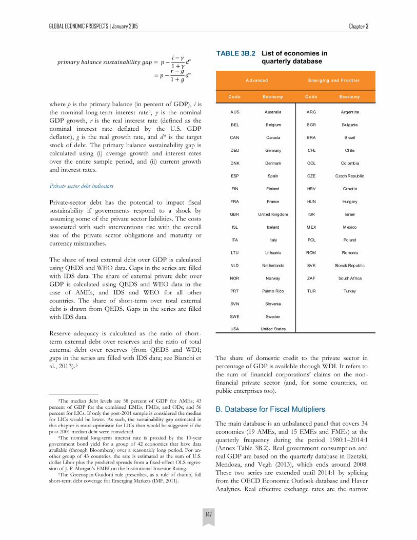
GLOBAL ECONOMIC PROSPECTS | January 2015 Chapter 3
147
where p is the primary balance (in percent of GDP), i is
the nominal long-term interest rate4, γ is the nominal
GDP growth, r is the real interest rate (defined as the
nominal interest rate deflated by the U.S. GDP
deflator), g is the real growth rate, and d* is the target
stock of debt. The primary balance sustainability gap is
calculated using (i) average growth and interest rates
over the entire sample period, and (ii) current growth
and interest rates.
Private sector debt indicators
Private-sector debt has the potential to impact fiscal
sustainability if governments respond to a shock by
assuming some of the private sector liabilities. The costs
associated with such interventions rise with the overall
size of the private sector obligations and maturity or
currency mismatches.
The share of total external debt over GDP is calculated
using QEDS and WEO data. Gaps in the series are filled
with IDS data. The share of external private debt over
GDP is calculated using QEDS and WEO data in the
case of AMEs, and IDS and WEO for all other
countries. The share of short-term over total external
debt is drawn from QEDS. Gaps in the series are filled
with IDS data.
Reserve adequacy is calculated as the ratio of short-
term external debt over reserves and the ratio of total
external debt over reserves (from QEDS and WDI;
gaps in the series are filled with IDS data; see Bianchi et
al., 2013).5
The share of domestic credit to the private sector in
percentage of GDP is available through WDI. It refers to
the sum of financial corporations’ claims on the non-
financial private sector (and, for some countries, on
public enterprises too).
B. Database for Fiscal Multipliers
The main database is an unbalanced panel that covers 34
economies (19 AMEs, and 15 EMEs and FMEs) at the
quarterly frequency during the period 1980:1–2014:1
(Annex Table 3B.2). Real government consumption and
real GDP are based on the quarterly database in Ilzetzki,
Mendoza, and Vegh (2013), which ends around 2008.
These two series are extended until 2014:1 by splicing
from the OECD Economic Outlook database and Haver
Analytics. Real effective exchange rates are the narrow
3The median debt levels are 58 percent of GDP for AMEs; 43 percent of GDP for the combined EMEs, FMEs, and ODs; and 56 percent for LICs. If only the post-2001 sample is considered the median for LICs would be lower. As such, the sustainability gap estimated in this chapter is more optimistic for LICs than would be suggested if the post-2001 median debt were considered.
4The nominal long-term interest rate is proxied by the 10-year government bond yield for a group of 42 economies that have data available (through Bloomberg) over a reasonably long period. For an-other group of 43 countries, the rate is estimated as the sum of U.S. dollar Libor plus the predicted spreads from a fixed-effect OLS regres-sion of J. P. Morgan’s EMBI on the Institutional Investor Rating.
5The Greenspan-Guidotti rule prescribes, as a rule of thumb, full short-term debt coverage for Emerging Markets (IMF, 2011).
List of economies in quarterly database
TABLE 3B.2
C o d e Eco no my C o d e Eco no my
AUS Australia ARG Argent ina
BEL Belgium BGR Bulgaria
CAN Canada BRA Brazil
DEU Germany CHL Chile
DNK Denmark COL Colombia
ESP Spain CZE Czech Republic
FIN Finland HRV Croat ia
FRA France HUN Hungary
GBR United Kingdom ISR Israel
ISL Iceland M EX M exico
ITA Italy POL Poland
LTU Lithuania ROM Romania
NLD Netherlands SVK Slovak Republic
NOR Norway ZAF South Africa
PRT Puerto Rico TUR Turkey
SVN Slovenia
SWE Sweden
USA United States
A d vanced Emerg ing and F ro nt ier
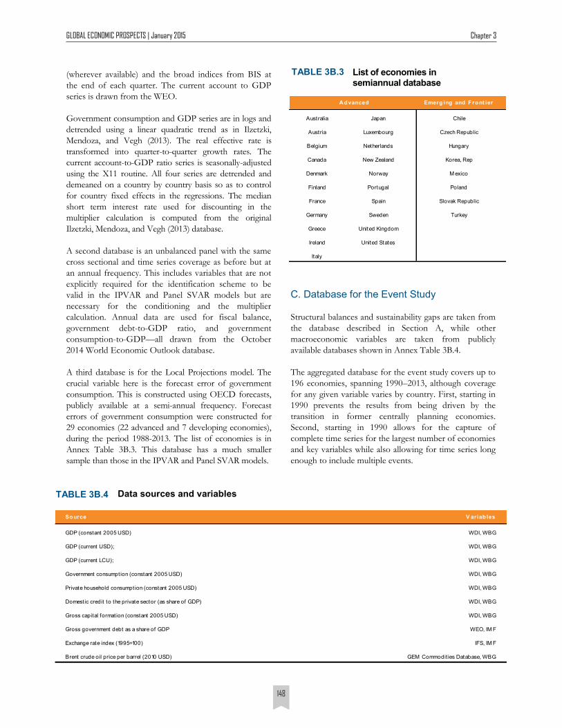
GLOBAL ECONOMIC PROSPECTS | January 2015 Chapter 3
148
(wherever available) and the broad indices from BIS at
the end of each quarter. The current account to GDP
series is drawn from the WEO.
Government consumption and GDP series are in logs and
detrended using a linear quadratic trend as in Ilzetzki,
Mendoza, and Vegh (2013). The real effective rate is
transformed into quarter-to-quarter growth rates. The
current account-to-GDP ratio series is seasonally-adjusted
using the X11 routine. All four series are detrended and
demeaned on a country by country basis so as to control
for country fixed effects in the regressions. The median
short term interest rate used for discounting in the
multiplier calculation is computed from the original
Ilzetzki, Mendoza, and Vegh (2013) database.
A second database is an unbalanced panel with the same
cross sectional and time series coverage as before but at
an annual frequency. This includes variables that are not
explicitly required for the identification scheme to be
valid in the IPVAR and Panel SVAR models but are
necessary for the conditioning and the multiplier
calculation. Annual data are used for fiscal balance,
government debt-to-GDP ratio, and government
consumption-to-GDP—all drawn from the October
2014 World Economic Outlook database.
A third database is for the Local Projections model. The
crucial variable here is the forecast error of government
consumption. This is constructed using OECD forecasts,
publicly available at a semi-annual frequency. Forecast
errors of government consumption were constructed for
29 economies (22 advanced and 7 developing economies),
during the period 1988-2013. The list of economies is in
Annex Table 3B.3. This database has a much smaller
sample than those in the IPVAR and Panel SVAR models.
List of economies in
semiannual database
TABLE 3B.3
Emerg ing and F ront ier
Australia Japan Chile
Austria Luxembourg Czech Republic
Belgium Netherlands Hungary
Canada New Zealand Korea, Rep
Denmark Norway M exico
Finland Portugal Poland
France Spain Slovak Republic
Germany Sweden Turkey
Greece United Kingdom
Ireland United States
Italy
A dvanced
Data sources and variables TABLE 3B.4
Source V ariab les
GDP (constant 2005 USD) WDI, WBG
GDP (current USD); WDI, WBG
GDP (current LCU); WDI, WBG
Government consumption (constant 2005 USD) WDI, WBG
Private household consumption (constant 2005 USD) WDI, WBG
Domestic credit to the private sector (as share of GDP) WDI, WBG
Gross capital formation (constant 2005 USD) WDI, WBG
Gross government debt as a share of GDP WEO, IM F
Exchange rate index (1995=100) IFS, IM F
Brent crude oil price per barrel (2010 USD) GEM Commodit ies Database, WBG
C. Database for the Event Study
Structural balances and sustainability gaps are taken from
the database described in Section A, while other
macroeconomic variables are taken from publicly
available databases shown in Annex Table 3B.4.
The aggregated database for the event study covers up to
196 economies, spanning 1990–2013, although coverage
for any given variable varies by country. First, starting in
1990 prevents the results from being driven by the
transition in former centrally planning economies.
Second, starting in 1990 allows for the capture of
complete time series for the largest number of economies
and key variables while also allowing for time series long
enough to include multiple events.
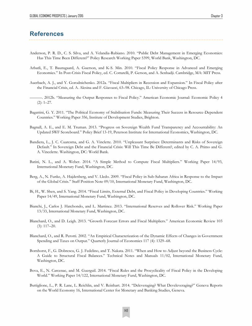
GLOBAL ECONOMIC PROSPECTS | January 2015 Chapter 3
149
Anderson, P. R. D., C. S. Silva, and A. Velandia-Rubiano. 2010. “Public Debt Management in Emerging Economies:
Has This Time Been Different?” Policy Research Working Paper 5399, World Bank, Washington, DC.
Arbatli, E., T. Baunsgaard, A. Guerson, and K-S. Min. 2010. “Fiscal Policy Response in Advanced and Emerging
Economies.” In Post-Crisis Fiscal Policy, ed. C. Cottarelli, P. Gerson, and A. Senhadji. Cambridge, MA: MIT Press.
Auerbach, A. J., and Y. Gorodnichenko. 2012a. “Fiscal Multipliers in Recession and Expansion.” In Fiscal Policy after
the Financial Crisis, ed. A. Alesina and F. Giavazzi, 63–98. Chicago, IL: University of Chicago Press.
———. 2012b. “Measuring the Output Responses to Fiscal Policy.” American Economic Journal: Economic Policy 4
(2): 1–27.
Bagattini, G. Y. 2011. “The Political Economy of Stabilisation Funds: Measuring Their Success in Resource-Dependent
Countries.” Working Paper 356, Institute of Development Studies, Brighton.
Bagnall, A. E., and E. M. Truman. 2013. “Progress on Sovereign Wealth Fund Transparency and Accountability: An
Updated SWF Scoreboard.” Policy Brief 13-19, Peterson Institute for International Economics, Washington, DC.
Bandiera, L., J. C. Cuaresma, and G. A. Vinclette. 2010. “Unpleasant Surprises: Determinants and Risks of Sovereign
Default.” In Sovereign Debt and the Financial Crisis: Will This Time Be Different?, edited by C. A. Primo and G.
A. Vincelette. Washington, DC: World Bank.
Batini, N. L., and A. Weber. 2014. “A Simple Method to Compute Fiscal Multipliers.” Working Paper 14/93,
International Monetary Fund, Washington, DC.
Berg, A., N. Funke, A. Hajdenberg, and V. Lledo. 2009. “Fiscal Policy in Sub-Saharan Africa in Response to the Impact
of the Global Crisis.” Staff Position Note 09/10, International Monetary Fund, Washington, DC.
Bi, H., W. Shen, and S. Yang. 2014. “Fiscal Limits, External Debt, and Fiscal Policy in Developing Countries.” Working
Paper 14/49, International Monetary Fund, Washington, DC.
Bianchi, J., Carlos J. Hatchondo, and L. Martinez. 2013. “International Reserves and Rollover Risk.” Working Paper
13/33, International Monetary Fund, Washington, DC.
Blanchard, O., and D. Leigh. 2013. “Growth Forecast Errors and Fiscal Multipliers.” American Economic Review 103
(3): 117–20.
Blanchard, O., and R. Perotti. 2002. “An Empirical Characterization of the Dynamic Effects of Changes in Government
Spending and Taxes on Output.” Quarterly Journal of Economics 117 (4): 1329–68.
Bornhorst, F., G. Dobrescu, G. J. Fedelino, and T. Nakata. 2011. “When and How to Adjust beyond the Business Cycle:
A Guide to Structural Fiscal Balances.” Technical Notes and Manuals 11/02, International Monetary Fund,
Washington, DC.
Bova, E., N. Carcenac, and M. Guerguil. 2014. “Fiscal Rules and the Procyclicality of Fiscal Policy in the Developing
World.” Working Paper 14/122, International Monetary Fund, Washington, DC.
Buttiglione, L., P. R. Lane, L. Reichlin, and V. Reinhart. 2014. “Deleveraging? What Develeveraging?” Geneva Reports
on the World Economy 16, International Center for Monetary and Banking Studies, Geneva.
149
References
GLOBAL ECONOMIC PROSPECTS | January 2015 Chapter 3
150
Calderon, C., and K. Schmidt-Hebbel. 2008. “Business Cycles and Fiscal Policies: the Role of Institutions and Financial
Markets.” Working Paper 481, Central Bank of Chile, Santiago.
Canzoneri, M., F. Collard, H. Dellas, B. Diba. 2012. “Fiscal Multipliers in Recessions.” Universität Bern
Diskussionsschriften 1204, University of Bern.
Christiano, L., M. Eichenbaum, and S. Rebelo. 2011. “When Is the Government Spending Multiplier Large?” Journal of
Political Economy 119 (1): 78–21.
Ciarlone, A., and G. Trebeschi. 2006. “Designing an Early Warning System for Debt Crises.” Emerging Markets Review
6 (2005): 376–95.
Coenen, Günter, Christopher J. Erceg, Charles Freedman, Davide Furceri, Michael Kumhof, René Lalonde, Douglas
Laxton, Jesper Lindé, Annabelle Mourougane, Dirk Muir, Susanna Mursula, Carlos de Resende, John Roberts,
Werner Roeger, Stephen Snudden, Mathias Trabandt, and Jan in’t Veld. 2012. “Effects of Fiscal Stimulus in
Structural Models.” American Economic Journal: Macroeconomics 4 (1): 22–68.
Corsetti, G., K. Kuester, A. Meier, and G. J. Müller. 2013. “Sovereign Risk, Fiscal Policy, and Macroeconomics.”
Economic Journal 123 (566): F99–F132.
Cuadra, G., J. M. Sanchez, and H. Sapriza. 2010. “Fiscal Policy and Default Risk in Emerging Markets.” Review of
Economic Dynamics 13 (2): 305–73.
Debrun, X., and A. Schaechte. 2014. “Institutional Reforms and Fiscal Adjustment.” In Post-Crisis Fiscal Policy, ed. C.
Cottarelli, P. Gerson, and A. Senhadji, 485–514. Cambridge, MA: MIT Press.
Dell’Erba, S., R. Hausmann, and U. Panizza. 2013. “Debt Levels, Debt Composition, and Sovereign Spreads in
Emerging and Advanced Economies.” Oxford Review of Economic Policy 29 (3): 518–47.
Detragiache, E., and A. Spilibergo. 2004. “Empirical Models of Short-Term Debt and Crises: Do They Rest the Creditor
Run Hypothesis?” European Economic Review 48 (2): 379–89.
Didier, T., C. Hevia, and S. L. Schmukler. 2012. “How Resilient and Countercyclical Were Emerging Economies during
the Global Financial Crisis?” Journal of International Money and Finance 31 (8): 2052–77.
Eden, M., and A. C. Kraay. 2014. “‘Crowding in’ and the Returns to Government Investment in Low-Income
Countries.” Policy Research Working Paper 6781, World Bank, Washington DC.
Eichengreen, B., and R. Hausmann. 1999. “Exchange Rates and Financial Fragility.” Proceedings from the Economic
Policy Symposium, Federal Reserve Bank of Kansas City, Jackson Hole, WY, August 26–28.
Eichengreen, B., R. Hausmann, and U. Panizza. 2009. “Currency Mismatches, Debt Intolerance, and Original Sin: Why
They Are Not the Same and Why It Matters.” In Capital Controls and Capital Flows in Emerging Markets: Policies,
Practices, and Consequences, edited by S. Edwards. National Bureau of Economic Research, Cambridge, MA.
Eskesen, L. L. 2009. “Countering the Cycle—The Effectiveness of Fiscal Policy in Korea.” Working Paper 09/249,
International Monetary Fund, Washington, DC.
Fardoust, S., J. Y. Lin, and X. Luo. 2012. “Demystifying China’s Fiscal Stimulus.” Policy Research Working Paper 6221,
World Bank, Washington, DC.
Fasano, U. 2000. “Review of the Experience with Oil Stabilization and Savings Funds in Selected Countries.” Working
Paper 00/112, International Monetary Fund, Washington, DC.
150
GLOBAL ECONOMIC PROSPECTS | January 2015 Chapter 3
151
Fatás, A. and I. Mihov. 2012. “Fiscal Policy as a Stabilization Tool.” Discussion Paper, Center for Economic Policy Research.
Frankel, J. 2011. “A Solution to Fiscal Procyclicality: The Structural Budget Institutions Pioneered by Chile.” Journal
Economía Chilena 14 (2): 39–78.
Frankel, J. A., C. A. Végh, and G. Vuletin. 2013. “On Graduation from Fiscal Procyclicality.” Journal of Development
Economics 100 (1): 32–47.
Gill, I. S., I. Izviorski, W. van Eeghen, and D. De Rosa. 2014. Diversified Development: Making the Most of Natural
Resources in Eurasia. Washington, DC: World Bank.
Grigoli, F., Z. Mills, M. Verhoeven, and R. Vlaicu. 2012. “MTEFs and Fiscal Performance: Panel Data Evidence.” Policy
Research Working Paper 6186, World Bank, Washington, DC.
Guajardo, J. C., D. Leigh, and A. Pescatori. 2014. “Expansionary Austerity? International Evidence.” Journal of the
European Economic Association 12 (4): 949–68.
Harding, D., and A. Pagan. 2002. “Dissecting the Cycle: A Methodological Investigation.” Journal of Monetary
Economics 49 (2): 365–81.
Hausmann, R., and U. Panizza. 2011. “Redemption or Abstinence? Original Sin, Currency Mismatches, and Counter
Cyclical Policies in the New Millennium.” Journal of Globalization and Development 2 (1): 1–35.
Heller, P. S. 2005. “Understanding Fiscal Space.” Policy Discussion Paper 05/04, International Monetary Fund,
Washington, DC.
Holmes, M., and A. Evans. 2003. A Review of Experience in Implementing Medium Term Expenditure Frameworks in
a PRSP Context: A Synthesis of Eight Country Studies. London: Overseas Development Institute.
IDB (Inter-American Development Bank) 2014. 2014 Latin America and Caribbean Macroeconomic Report.
Washington, DC: IDB.
Ilzetzki, E., E. Mendoza, and C. Végh. 2013. “How Big (Small?) Are Fiscal Multipliers?” Journal of Monetary
Economics 60 (2): 239–54.
IMF (International Monetary Fund). 2002. Assessing Sustainability. Washington, DC: IMF.
———. 2009. “Chile: 2009 Article IV Consultation.” Country Report 09/271, IMF, Washington, DC.
———. 2010. “World Economic Outlook.” October, IMF, Washington, DC.
———. 2011. Assessing Reserve Adequacy. Washington, DC: IMF.
———. 2012. “World Economic Outlook.” October, IMF, Washington, DC.
———. 2013. “Heavily Indebted Poor Countries (HIPC) Initiative and Multilateral Debt Relief Initiative (MDRI):
Statistical Update.” IMF, Washington, DC.
———. 2014a. “2014 Spillover Report.” Policy Paper, IMF, Washington, DC.
———. 2014b. “Debt Relief under the Heavily Indebted Poor Countries (HIPC) Initiatives Factsheet.” IMF,
Washington, DC. https://www.imf.org/external/np/exr/facts/pdf/hipc.pdf.
151
GLOBAL ECONOMIC PROSPECTS | January 2015 Chapter 3
152
———. 2014c. “World Economic Outlook.” October, IMF, Washington, DC.
———. 2014d. “Fiscal Monitor.” October, IMF, Washington, DC.
Jedidi, O. 2013. “Predicting Sovereign Debt Crises: A Panel Data Approach Using Composite Indices.” Mimeo,
University of Rennes.
JP Morgan. 2014. “EMBI Global and EMBI Global Diversified: Rules and Methodology.” Methodology Brief, JP
Morgan.
Kohler, M. 2010. “Exchange Rates during Financial Crises.” BIS Quarterly Review 2010(March).
Kraay, A. C. 2012. “How Large Is the Government Spending Multiplier? Evidence from World Bank Lending.”
Quarterly Journal of Economics 127 (2): 829–87.
———. 2014. “Government Spending Multipliers in Developing Countries: Evidence from Lending by Official
Creditors.” American Economic Journal: Macroeconomics 6 (4): 170–208.
Kraay, A. C., and V. Nehru. 2006. “When Is External Debt Sustainable?” World Bank Economic Review 20 (3): 341–65.
Kraay, A. C., and L. Serven. 2013. “Fiscal Policy as Tool for Stabilization in Developing Countries.” Background Note
for 2014 World Development Report: Managing Risks for Development, Washington, DC, World Bank.
Krugman, P., 2013. “Currency Regimes, Capital Flows, and Crises,” Paper presented at the 14th Jacques Polak Annual
Research Conference, IMF.
Laeven, L., and F. Valencia. 2013. “Systemic Banking Crises Database.” IMF Economic Review 2013 (61): 225–70.
Le Houerou, P., and Taliercio. 2002. “Medium Term Expenditure Frameworks: From Concept to Practice, Preliminary
Lessons from Africa.” Africa Region Working Paper 28, World Bank, Washington, DC.
Ley, E. 2009. “Fiscal Policy for Growth.” PREM Note131, World Bank, Washington, DC.
Ley, E., and F. Misch. 2014. “Output Data Revisions in Low-Income Countries.” Paper presented at the joint RES-SPR
conference on “Macroeconomic Challenges Facing Low-Income Countries,” Washington, DC, January 30–31.
Manasse, P., and N. Roubini. 2009. “‘Rules of Thumb’ for Sovereign Debt Crises.” Journal of International Economics
78 (2): 192–205.
Mineshima, A., M. Poplawski-Ribeiro, and A. Weber. 2014. “Size of Fiscal Multipliers.” In Post-Crisis Fiscal Policy, ed.
C. Cottarelli, P. Gerson, and A. Senhadji, 315–72. Cambridge, MA: MIT Press.
Nickel, R., and A. Tudyka. 2013. “Fiscal Stimulus in Times of High Debt: Reconsidering Multipliers and Twin Deficits.”
Working Paper 1513, European Central Bank, Frankfurt.
Ostry, J. D., A. R. Ghosh, J. I. Kim, and M. S. Qureshi. 2010. “Fiscal Space.” Staff Position Note 10/11, International
Monetary Fund, Washington, DC.
Perotti, R. 1999. “Fiscal Policy in Good Times and Bad.” Quarterly Journal of Economics 114 (4): 1399–1436.
———. 2007. “Fiscal Policy in Developing Countries: A Framework and Some Questions.” Policy Research Working
Paper 4365, World Bank, Washington, DC.
152
GLOBAL ECONOMIC PROSPECTS | January 2015 Chapter 3
153
Primiceri, G. E. 2005. “Time Varying Structural Vector Autoregressions and Monetary Policy.” Review of Economic
Studies 72 (3): 821–52.
Ramey, V. 2011. “Identifying Government Spending Shocks: It’s All in the Timing.” Quarterly Journal of Economics
126 (1): 1–50.
Ramey, V., and M. D. Shapiro. 1998. “Costly Capital Reallocation and the Effects of Government Spending.” Carnegie-
Rochester Conference Series on Public Policy 48 (1998): 145–94.
Reinhart, C.M and K.S. Rogoff. 2009. This Time is Different: Eight Centuries of Financial Folly. Princeton, NJ:
Princeton University Press.
———. 2011. “From Financial Crash to Debt Crash.” American Economic Review 101 (5): 1676–1706.
Reinhart, C. M., K. S. Rogoff, and M. A. Savastano. 2003. “Debt Intolerance.” Working Paper 9908, National Bureau of
Economic Research, Cambridge, MA.
Rendahl, P. 2012. “Fiscal Policy in an Unemployment Crisis.” Working Papers in Economics 1211, University of
Cambridge.
Riera-Crichton, D., C. A. Végh, and G. Vuletin. 2012. “Tax Multipliers: Pitfalls in Measurement and Identification.”
Working Paper 18497, National Bureau of Economic Research, Cambridge, MA.
———. 2014. “Fiscal Multipliers in Recessions and Expansions: Does It Matter Whether Government Spending Is
Increasing or Decreasing?” Policy Research Working Paper 6993, World Bank, Washington, DC.
Schaechter, A., T. Kinda, N. Budina, and A. Weber. 2012. “Fiscal Rules in Response to the Crisis—Toward the “Next-
Generation” Rules: A New Dataset. Working Paper 12/187, International Monetary Fund, Washington, DC.
Schmidt-Hebbel, K. 2012a. “The Political Economy of Distribution and Growth in Chile.” Working Paper 417, Instituto
de Economía, Pontificia Universidad Católica de Chile.
———. 2012b. “Fiscal Institutions in Resource-Rich Economies: Lessons from Chile and Norway.” Working Paper
416, Instituto de Economía, Pontificia Universidad Católica de Chile, Santiago, Chile.
Snudden, S. 2013. “Countercyclical Fiscal Rules for Oil Exporting Countries.” Working Paper 13/229, International
Monetary Fund, Washington, DC.
Sugawara, N. 2014. “From Volatility to Stability in Expenditure: Stabilization Funds in Resource-Rich Countries.”
Working Paper 14/43, International Monetary Fund, Washington, DC.
Sutherland, A. J. 1997. “Fiscal Crises and Aggregate Demand: Can High Public Debt Reverse the Effects of Fiscal
Policy?” Journal of Public Economics 65 (2): 147–62.
Towbin, P., and S. Weber. 2013. “Limits of Floats: The Role of Foreign Currency Debt and Import Structure.” Journal
of Development Economics 101 (March 2013): 179–94.
UN. 2011. The Global Social Crisis: Report on the World Social Situation 2011. New York: United Nations.
Végh, C., and G. Vuletin. 2013. The Road to Redemption: Policy Response to Crises in Latin America. Washington, DC:
International Monetary Fund.
World Bank. 2013a. Global Economic Prospects June 2013: Less Volatile, but Slower Growth. Washington, DC: World
153
GLOBAL ECONOMIC PROSPECTS | January 2015 Chapter 3
154
Bank.
———. 2013b. World Development Report 2014: Risk and Opportunity—Managing Risk for Development.
Washington, DC: World Bank.
———. 2013c. Beyond the Annual Budget. Washington, DC: World Bank.
———. 2014a. Global Economic Prospects January 2014: Coping with Policy Normalization in High-Income
Countries. Washington, DC: World Bank.
———. 2014b. East Asia Economic Update October 2014: Enhancing Competitiveness in an Uncertain World.
Washington, DC: World Bank.
———. 2014c. Global Monitoring Report 2014/2015: Ending Poverty and Sharing Prosperity. Washington, DC: World
Bank.
———. 2014d. A Measured Approach to Ending Poverty and Boosting Shared Prosperity: Concepts, Data, and the
Twin Goals. Washington, DC: World Bank.
154