GLOBAL CHANGE AND FORESTRY:

ECONOMIC AND POLICY IMPLICATIONS

Proceedings of the 2007 Southern Forest Economics Workshop March 4-6, 2007

San Antonio, Texas

Editor

Jianbang Gan Department of Ecosystem Science and Management

Texas A&M Univeristy

February 2008

i

Preface

The 2007 Southern Forest Economics Workshop (SOFEW) was held in San Antonio, Texas, with a theme topic of Global Change and Forestry: Economic and Policy Implications. It drew participants from the US, Canada, and outside of North America. Participants were welcomed by Dr. Steve Whisenant, Professor and Head of the Department of Ecosystem Science and Management at Texas A&M. Drs. Bruce A. McCarl and Peter J. Ince gave keynote speeches respectively on global climate change and global change in wood fiber markets, probably two of the most important global changes that would have profound impacts on forest resource management in the US South and elsewhere. Drs. Gregory S. Amacher, David H. Newman, David N. Wear, and Daowei Zhang shared with the participants their insightful perspectives on the past, present, and future of forest economics and policy research in a panel presentation. Followed these two general sessions were concurrent paper and poster sessions. This volume of proceedings contains the papers presented in the concurrent and poster sessions of the conference. These papers covered a wide spectrum of forest economics and policy issues in North America and beyond. They were grouped into nine parts: climate change and land use, forest products markets, nonindustrial private forests, forest bioenergy, economic impact and development, multiple uses and valuation, forest conservation, investment and mill location, and poster abstracts. Many individuals contributed to this conference. First, I would like to thank Drs. Steven H. Bullard, Frederick W. Cubbage, Stephen C. Grado, Don G. Hodges, Bruce A. McCarl, Ian A. Munn, David H. Newman, David N. Wear, and Steve Whisenant for their advice in planning the conference. Second, I am grateful to the two keynote speakers, the four panelists, and all presenters and participants, whose participation and contributions were vital to the success of this conference. Finally, my appreciation also goes to Dr. Ian A. Munn, Dr. Weihua Xu, Chyrel Mayfield, Adam Jarrett, Hsiaohsuan Wang, and Lindsey M. Eidner, who provided invaluable assistance with conference logistics. Sincerely, Jianbang Gan

ii

Table of Contents

Preface …………………………………………………………………………………………i

I. Climate Change and Land Use

Forest Management Adaptation to Climate Change and Extreme Events …………...…....1

Jin Huang and Bob Abt A Case Study to Examine How a Forestry Firm Might Respond to Different Mechanism to Encourage Carbon Sequestration …………………………………….……2

Patrick Asante Impact of Population Growth and Urban Sprawl on Land Use and Forest Type Dynamics along Urban-rural Gradient ……………………………………………....…….3

Maksym Polyakov and Daowei Zhang Impacts of Climate Change on Tennessee Forests………………………………….……13

Donald G. Hodges, Virginia H. Dale, and Jonah Fogel

II. Forest Products Markets How Competitive is the Wood Supply Chain in the U.S. South?………………………..14

Jacek P. Siry, W. Dale Greene, Thomas G. Harris, Jr., and Robert L. Izlar Is the Current Poor Market for Hardwood Lumber in North Carolina, Virginia, and West Virginia Temporary? …………………………………………………………..15

William Luppold and Matthew Bumgardner An Econometric Analysis of Pine Pulpwood Market in the Southern US……………….23

Xianchun Liao and Yaoqi Zhang A Review of Econometric Models for Softwood Lumber ……………………………….34

Nianfu Song and Sun Joseph Chang

Measuring Oligopsony and Oligopony Power in the U.S. Paper Industry ………………35 Bin Mei and Changyou Sun Testing the Efficiency of Spatial Arbitrage between North American Softwood Lumber Markets of Homogeneous Products ………………………………….46 Chander Shahi and Shashi Kant

iii

A Time Series Analysis of Lumber Market in US South ………………………………..47 Ram Pandit and Indrajit Mujumdar An Analysis of Quarterly Composite Hardwood Sawtimber Price Indices: 1998-2006 ………………………………………………………………………………..48 Chris Zinkhan, Blake Stansell, and Thresa Henderson Hardwood Lumber Demand:1963 to 2002 ……………………………………………....49 William Luppold and Matthew Bumgardner

III. Nonindustrial Private Forests Unintended Consequences: Effect of the American Jobs Creation Act Reforestation Incentives on Family Forest Owners in the South ………………………..56 John L. Greene and Thomas J. Straka Impacts of Timberland Ownership on Stumpage Market in the US South………………63 Yaoqi Zhang and Xianchun Liao Forest Management Decisions of Nonindustrial Private Forest Landowners of West Virginia …………………………………………………………………………….74 Sudiksha Joshi and Kathryn G. Arano Nonindustrial Private Forest Landowners’ Participation in Mississippi Forest Resource Development Program…………………………………………………………75 Xing Sun, Changyou Sun, Ian A. Munn, and Anwar Hussain How Long Do NIPF Landowners Wait to Reforest after Harvesting? …………………..87 Xing Sun, Ian A. Munn, and Changyou Sun Analysis of Family Forest Holdings Structure in the United States ……………………..95 Yaoqi Zhang, Xianchun Liao, and Brett J. Butler Timber Harvest Behavior of Nonindustrial Private Forest (NIPF) Landowners Facing Uncertainty from an Insect Pest: The Case of the Red Oak Borer……………...104 G.C. Surendra and Sayeed R. Mehmood Discriminating Family Forest Owner Groups Using a Non-parametric Approach ………………………………………………………………………………..105 Indrajit Majumdar, Lawrence D. Teeter, and Brett J. Butler

IV. Forest Bioenergy

Biofuel Production Impact on the Management of Southern Pine Plantation in Mississippi ……………………………………………………………………….……..111 Zhimei Guo, Donald L. Grebner, Changyou Sun, and Stephen C. Grado

iv

Woody Biomass Feedstock Supplies and Management for Bioenergy in Southwestern Mississippi……………………………………………………………….121 Gustavo Perez-Verdin, Donald Grebner, Changyou Sun, Ian Munn, Emily

Schultz, and Thomas Matney A Forest Product/Bioenergy Mill Location and Decision Support System Based on a County-level Forest Inventory and Geo-spatial Information ………………131 T. Luke Jones, Emily B. Schultz, Thomas G. Matney, Donald L. Grebner,

and David L. Evans Logging Residues as a Source of Bioenergy Feedstock ………………………………..139 Robert K. Grala, Laura A. Grace, and William B. Stuart To Burn or Not to Burn …………………………………………………………………140 Sun Joseph Chang

V. Economic Impact and Development Economic Impacts Associated with Mississippi Outfitters and Their Clientele ………..141

Anwar Hussain and Ian A. Munn Economic Impacts of Two Birding Festivals in Mississippi …………………………...142 Marcus K. Measells and Stephen C. Grado An Introduction to the Southern US Wood Supply System: A Value Chain Approach ………………………………………………………………………………..150 Clayton B. Altizer Forest-based Economic Development in Arkansas: A Case for the Forest Products Industry………………………………………………………………………..160 Matthew H. Pelkki Development of a South-wide Forest Economics Dataset for the Southern Forest Research Partnership …………………………………………………………….161 Matthew Pelkki Economic Impact of the Forest Policy in Uruguay ……………………………………..162 Virginia Morales

VI. Multiple Uses and Valuation Recreational Visitation Patterns on Lake Impoundments in East-Central Mississippi………………………………………………………………………………163 Jon P. Rezek and Stephen C. Grado

v

Factors Determining Per Acre Market Value of Hunting Leases on Sixteenth Section Lands in Mississippi …………………………………………………………...171 Jacob Rhyne Influence of Field Windbreaks on Landscape Aesthetics: Preliminary Results ………..178 Robert K. Grala, John C. Tyndalland, and Carl W. Mize

Willingness-to-pay Assessment of Visitors to an Off-highway Vehicle Recreation Area: An Individual Travel Cost Method Approach ……………………….179 Gregory Parent, Janaki Alavalapati, Taylor Stein, and Chris Reed Role of Natural Amenity Resources in Retiree Location Choice Behavior: Potential Concern for Economic Growth and Ecological Disturbance in Rural America …………………………………………………………………………………180 Neelam C. Poudyal, Donald G. Hodges, and Ken Cordell Nonmarket Valuation Based on Market Information: An Application to U.S. Forest Resources ………………………………………………………………………..181 Jianhua Cao and Daowei Zhang

VII. Forest Conservation

Factor Driving Deforestation in Common-pool Resources in Durango, Mexico ………182

Gustavo Perez-Verdin, Yeon-Su Kim, Denver Hospodarsky, and Aregai Tecle

Determinants of Forest Preservation …………………………………………………...183 J.A. Anderson1, M.K. Luckert, and W.L. Adamowicz A Marginal Cost Analysis of Trade-offs in Preservation of Old Growth in an Even Aged Boreal Forest of Ontario …………………………………………………...185 Rajender P. Khajuria and Susanna Laaksonen-Craig Globalization, Market Economy and Tropical Deforestation: Evidence from Southwest China ………………………………………………………………………..186 Youxin Ma, Yaoqi Zhang, Hongmei Li, Wenjun Liu, and Min Cao Performance Bonding and Reforestation of Surface Mined Lands …………………….187 Jay Sullivan and Greg Amacher Evaluation of Cogongrass Control Techniques for Nonindustrial Private Landowners in Mississippi ……………………………………………………………..188

Jon D. Prevost, Donald L. Grebner, Jeanne C. Jones, Stephen C. Grado, Keith L. Belli, and John Byrd

vi

VIII. Investment and Mill Location Investment Analysis and Timberland Portfolios in the US …………………………….194 Xianchun Liao and Yaoqi Zhang An Empirical Analysis of Timberland Ownership and Corporate Financial Performance for Forestry Industries in the U.S. ………………………………………..205 Yanshu Li and Daowei Zhang The Location Theory Dilemma in the Forest Products Industry: What Site-attributes Are Considered for the Establishment of Softwood Sawmills? ……………...206 Francisco X. Aguilar and Richard P. Vlosky

IX. Poster Abstracts

Measuring the Biological and Economic Effects of Wildlife Herbivory on Afforested Carbon Sequestration Sites in the Lower Mississippi Alluvial Valley …………………………………………………………………………………...207

Daniel C. Sumerall, Donald L. Grebner, Jeanne C. Jones, Keith L. Belli, Stephen C. Grado, and Richard P. Maiers

A Case Study to Examine How a Forestry Firm Might Respond to Different Mechanism to Encourage Carbon Sequestration ……………………………………….208 Patrick Asante Linking Attitude and Subjective Norm to Intention and Fire Use Behavior: The Case of the Wu-Lin district, Taiwan ……………………………………………….209 Hsiaohsuan Wang, Jianbang Gan, Chyirong Chiou, and Chauchin Lin An Evaluation of the Economic Potential of Surface Mined Areas for Tree Production ………………………………………………………………………………210

Adam Michels, Tamara Cushing, Christopher Barton, Jim Ringe, Patrick Angel, Rick Sweigard, and Donald Graves

Property Taxation and Forest Fragmentation in Kentucky Watersheds ………………..211 Scott Brodbeck and Tamara Cushing A Comparison of Taxes Incurred during the Production and Delivery of Hardwood Sawtimber in Kentucky, Maryland, Virginia, and West Virginia ………….212 Kathryn Arano and Stuart Moss Spatial Analysis of Economic Freedom, Corruption, and Species Imperilment at Cross-country Level ………………………………………………………………….213 Ram Pandit and David N. Laband

vii

Breeching the Biomass Barriers: Analyzing Policy and Cost Effectiveness for Wildfire Mitigation and Biomass Utilization …………………………………………..214 Adam Jarrett and Jianbang Gan

Conference Program ………………………………………………………………………..215 List of Participants ………………………………………………………………………….222

1

Forest Management Adaptation to Climate Change and Extreme Events

Jin Huang1, 2 and Bob Abt2

Abstract: The objective of this paper is to examine forest managers’ adaptation to climate change and climate-change-related discrete extreme events (e.g. hurricanes, floods, and wildfires) in the managed forests of the southern U.S. There is an extensive literature focused on agricultural adaptive response to climate change. There is also literature that examines forest ecosystem impacts of climate change and forest manager’s adaptation to risks from wildfires or other discrete events that are correlated with climate change. This paper will provide an integrated analysis of forest management response to a likely known trend in changing climate in addition to a lesser known risk from discrete events. Unlike agriculture with annual time steps, forest management occurs on a temporal scale that implies that decisions today will be influenced by climate change expectations 20 to 40 years in the future. The adaptive actions considered in this paper include choice of species, intermediate treatments (prescribed burning, fertilization), change of rotation age and purchase of forestry insurance. Adaptive actions are examined using two approaches; a Markov Decision Process (MDP) approach and Decision Simulation (DS) approach. In our DS model the probability density function of the timing of discrete events (including harvest) on a forest stand is developed and the benefit function is optimized with respect to the decision variables. The MDP approach models stochastic transition between different stand states. Forest managers’ decisions change the transition probabilities between stand states. Both methods are applied to the pine plantations in the southern eastern U.S. using Forest Inventory and Analysis (FIA) data. Results from the two models are examined and compared. One important contribution of this paper is that it studies human adaptation to both continuous climate change and discrete extreme events.

1 Corresponding author and presenter, jhuang@ncsu.edu. 2 Department of Forestry and Environmental Resources, College of Natural Resources, North Carolina State University.

2

A Case Study to Examine How a Forestry Firm Might Respond to Different Mechanism to Encourage Carbon Sequestration

Patrick Asante1

Abstract: Despite considerable interest in the potential for forests to sequester carbon, there is still a gap in knowledge when it comes to determining the effect of carbon credit trading on forestry firms as it relates to harvest/leave decisions, reforestation options, and afforestation of agricultural land. Managing forest for carbon budget may result in modifications to the way forests are managed in Canada depending on the incentives provided by carbon markets. Utilizing the southwestern portion of Daishowa-Marubeni International Ltd. (DMI) forest management area (FMA) in Peace River, Alberta, as a case study, from the perspective of a carbon credit supplier, a mathematical programming model is used to evaluate how carbon price, silvicultural practices, supply of carbon credits, and allowable annual cut regulations could affect a forestry firms decision to undertake enhanced carbon sequestration. The knowledge gained through this research will enter into national policy discussions regarding carbon management, and will inform relevant agencies about how forestry firms might respond to different mechanisms that seek to encourage carbon sequestration. Results and methods from this study should give forestry firms the building blocks to develop strategic plans for managing their forest for carbon budget. Keywords: Carbon sequestration, mathematical programming model, carbon sinks, carbon budget

1 University of Alberta, Canada, Patrick.Asante@afhe.ualberta.ca.

3

Impact of Population Growth and Urban Sprawl on Land Use and Forest Type Dynamics along Urban-rural Gradient*

Maksym Polyakov1, 2 and Daowei Zhang2

Abstract: In this study we applied a conditional logit model to determine factors affecting land cover change in three contiguous counties in West Georgia (Muscogee, Harris and Meriwether) during the period 1992-2001 and used this model to predict land cover changes during the period 2001-2021 based on the assumptions of population growth. Introduction

Land use changes, while driven by maximization of economic benefits to land owners, sometimes produce negative externalities such as air and water pollution, loss of biodiversity wildlife habitat fragmentation, and increased flooding. In the conditions when majority of land base is privately owned, like in the US South, it is important to understand how economic, social, environmental factors affect private landowners’ decisions concerning land use change. Most of existing studies of land use in the U.S. are based on the classic land use theory developed by David Ricardo and Johann von Thünen. This theory explains land use patterns in terms of relative rent to alternative land uses, which depends on land quality and location. Due to data limitations, majority of econometric land use studies utilize aggregate data describing areas or proportions of certain land use categories within well defined geographic area such as a county or other region as a function of socioeconomic variables and land characteristics aggregated at the level of geographic unit of observation (Alig and Healy 1987; Plantinga, Buongiorno, and Alig 1990; Stavins and Jaffe 1990). Some of the studies, employing aggregate data, model shares of exhaustive set of land use within specified land base using binomial or multinomial logit model of shares, which allows restricting shares to unity (Parks and Murray 1994; Hardie and Parks 1997; Ahn, Plantinga, and Alig 2000, Nagubadi and Zhang 2005; Zhang and Nagubadi 2005). Comparing pooled, fixed effects, and random effects specifications of the cross-sectional–time series land use shares model, Ahn, Plantinga, and Alig (2000) came to a conclusion that pooled specification does not adequately control for cross-sectional variation in dependent variables. As a result the models’ parameters measure a combination of spatial and temporal effects and cannot be used for the inferences regarding land use change of land use change predictions. They suggested that a specification with cross-sectional fixed effects provide a better measure of temporal relationship. However, the use of cross-sectional fixed effects requires relatively long time series and prevents the use of explanatory variables that do not have temporal variation (like land quality). These obstacles were overcome in some recent studies that use parcel-based observation of land characteristics in order to directly measure land use transitions. Depending on the number of land use categories considered (choices) they use * This study was supported by the National Research Initiative of the Cooperative State Research, Education and

Extension Service, USDA, Grant #USDA-2005-3540015262. 1 Corresponding author and presenter, polyama@auburn.edu, (334) 844 8061 (v), (334) 844 1084 (fax). 2 School of Forestry and Wildlife Sciences Building, Auburn University, AL 36849-5418.

4

binominal probit (Kline, Moses, and Alig 2001), or nested logit (Lubowski, Plantinga, and Stavins 2006) models. In this paper we evaluate the effect of urbanization on the changes between major categories of land cover/use and forest types using remotely sensed data. In the next section we describe study area. Then we lay out a simple discrete choice model of land use change and corresponding econometric model followed by description of data. Later section provides results of spatial conditional logit estimation of the model of land cover/use change. The concluding section presents prediction of land cover/use change for the next two decades. Study Area Our study area is in the Georgia Piedmont, a region that displays rapid development and ranks among the highest regions in terms of percentage increase in developed land area during the 1990s. Within this region we study land use change in three contiguous counties: Muscogee, Harris, and Meriwether. Despite being contiguous, these counties exhibit broad range of population pressure and patterns of land uses and land use change from urban (Muscogee county) to rural (Meriwether county). Columbus, located in Muscogee County, is the third largest city in Georgia. Muscogee County accounts for 80% of the population of tree county region. However during 1990s it had a moderate population growth. Population of Harris County, which is located north of Muscogee County and is becoming its bedroom community, had increased by one-third during the same period, while population of Meriwether County almost did not increase (Table 1). Table 1. Population and land use statistics in Harris, Meriwether and Muscogee counties Characteristics County Total Harris Meriwether Muscogee Population: Person, 2000 23,695 22,534 186,291 232,520 Person/km2, 2000 19 17 325 75 Annual % change, 1990-2000 3.3% 0.1% 0.4% 0.6% Agricultural lands: % of land base, 1997 6.3% 10.2% 5.5% 7.8% Annual % change, 1992-1997 -0.3% -3.1% -4.7% -2.5% Forest lands: % of land base, 1997 78.3% 80.5% 24.8% 69.3% Annual % change, 1992-1997 -0.4% 0.8% -2.1% 0.0% Developed lands: % of land base, 1997 6.9% 5.9% 29.8% 10.7% Annual % change, 1992-1997 4.6% 4.1% 3.8% 4.1%

Figure 1 shows density of population in 2000 and change of population density during 1990-2000 period. It reveals, that population increases around populated places and in the same time declines in the immediate proximity to centers of most populated places, especially Columbus. Furthermore, land is being converted to developed use at a greater rate than population is increasing. According to the data collected by National Resources Inventory (NRI), during the period 1992-1997 average annual increase of the area of developed land in these three counties was 4.1%, while average annual increase of population in 1990s was 0.6% (see Table 1). Most of developed land was converted from forest, however, due to simultaneous conversion of agricultural land to forest land, proportion of forest land did not significantly change, while

5

agricultural lands declined by one-third between 1987 and 1997. These patterns of population growth and land use change are reflection of discontinuous low density development that is often cited as urban sprawl (Bogue, 1956).

Gay

Shiloh

Woodbury

Hamilton

Columbus

Lone Oak

Bibb City

Manchester

Greenville

West Point

Waverly Hall

Warm Springs

Luthersville

Pine Mountain

Change of population density 1990-2000, person/km2< -100

-99.9 -- -10

-9.9 -- 9.9

10 -- 99.9

> 100

Gay

Shiloh

Woodbury

Hamilton

Columbus

Lone Oak

Bibb City

Manchester

Greenville

West Point

Waverly Hall

Warm Springs

Luthersville

Pine Mountain

Population density 2000, person/km20

1 - 10

11-50

51-100

101-500

501-2000

Georgia

Figure 1. Spatial patterns of level and change of population density in three West Georgia counties. The Theoretical Model Our modeling approach is based on the assumption that land use and land cover spatial patterns and their changes are results of decisions of the owners of individual land parcels or cells in the landscape. Land owner chooses to allocate a parcel of land of uniform quality to one of several possible alternative uses. We assume that a landowner’s decision is based on the maximization of net present value of future returns generated by the land. The owner’s expectations concerning future returns generated by different land uses are drawn from the characteristics of the parcel and historical returns. Let niW be the net present value of parcel n in use i which depends on characteristics of a parcel such as land quality and location, as well as economic conditions. Converting a parcel from use i to alternative use j also involves one time conversion cost nijC , which depends on land uses parcel is being converted from and to, on characteristics of a parcel,

6

as well as on institutional settings such as zoning regulations. Let |nj i nj ni nijU W W C= − − be the landowner’s utility of converting a parcel to new land use j conditional on current land use i. The parcel could be converted to land use j if |nj iU is positive. Furthermore, the parcel will be converted to the land use, for which utility of conversion is greater. Parcel will remain in current land use ( 0niiC = ; | 0ni iU = ) if | 0nj iU j i< ∀ ≠ . Neither return for each of the land uses, nor conversion costs are directly observable for individual parcels, however, there are observable attributes of plots nx , that are related to either returns or conversion costs. Furthermore, there might be spatial dependencies njZ across decision makers due to the fact that some of the spatially related factors affecting decisions are not observable directly, so that njinjinj VU ε+= || , where | ( , )nj i n niV V Z= x is the representative utility and njε captures the factors that are affecting utility, but not included into representative utility, and assumed to be random. The probability of converting parcel n to land use j is

| | |

| |

Prob( )

Prob( )nj i nj i nk i

nj i nj nk i nk

P U U k j

V V k jε ε

= > ∀ ≠

= + > + ∀ ≠ (1)

Depending on assumptions about the density distribution of random components of utility, several different discrete choice models could be derived from this specification (Train, 2003). Assuming random components are independent and identically distributed (iid) with a type I extreme value distribution, we obtain a conditional logit model (McFadden 1973):

||

|1

exp( )

exp( )

nj inj i J

nk ik

VP

V=

=

∑ (2)

Representative utility of converting parcel n from land use i to land use j could be expressed as a linear combination of observable attributes of plots ( nx ), land use specific parameters ( jβ ), transition specific parameter ( nijα ), and spatial dependencies across decision makers ( , 11

Snj ns sj tsZ yρ −==∑ ):

| , 11( ) ' ' Snj i n nij j n i n ns sj tsV V yα ρ −=

= = + − +∑x β x β x (3) where nsρ is a coefficient representing the influence parcel s has on parcel n and , 1sj ty − is equal to unity if parcel s was in land use j, and zero otherwise. In spatial statistics, ρ is usually takes a form of a negative exponential function of the distance ( nsD ) separating two units of observation:

7

exp nsns

Dρ λγ

⎛ ⎞= −⎜ ⎟

⎝ ⎠ (4)

And

, 1 , 11 1

exp expS S

ns nsnj j sj t j sj t

s s

D DZ y yλ λγ γ− −

= =

⎛ ⎞ ⎛ ⎞= − = −⎜ ⎟ ⎜ ⎟

⎝ ⎠ ⎝ ⎠∑ ∑ (5)

Substituting (3) and (5) into (2) obtain:

( )( )

( )( )( )( )

, 1 , 1 , 11, | , 1

, 1 , 1 , 111

, 1 , 11

, 1 , 111

exp ' '

exp ' '

exp ' exp

exp ' exp

Sij j n t i n t ns sj ts

nj t i t J Sij k n t i n t ns sk ts

k

Sij j n t j ns sj ts

J Sij j n t j ns sk ts

k

yP

y

D y

D y

α ρ

α ρ

α λ γ

α λ γ

− − −=−

− − −==

− −=

− −==

+ − +=

+ − +

+ + −=

+ + −

∑

∑ ∑

∑

∑ ∑

β x β x

β x β x

β x

β x

(6)

The estimation of spatial dependency ρ requires estimation of parameters jλ and γ . One of the ways to do this is obtaining γ through the search procedure over a range of numbers while estimating the value of jλ as standard parameters in conditional logit model (Mohammadian and Kanaroglu 2003). In our model of land use change, the observable attributes of plots ( ntx ) are conservation status, level of urbanization, elevation, slope, and distance to the nearest highway and the nearest road. Data To develop a model of land cover transitions we need information about land cover characteristics for a set of sample points in at least two points in time. We used two data sets: USGS National Land Cover Dataset for 1992 (NLCD 1992) based on satellite images taken around 1992, and NLCD 2001. However, there are several reasons why these datasets cannot be used directly to model land cover transition on a point (pixel) basis. First, these datasets use slightly different classification schemes; many land cover types of NLCD 1992 cannot be matched with land cover types of NLCD 2001. Second, the accuracy is not good enough to model land cover transition on a pixel basis. Finally, NLCD land cover classifications do not discriminate between development and transportation network and do not identify clearcuts and young plantations among other (non-forest) barren/grasses/shrubs land covers. Transportation infrastructure has distinctively different patterns of transition compare to the rest of developed uses, similarly clearcuts/young plantations has different land cover change patterns than non-forestry barren land, grasses, or shrubs. For these reasons we systematically selected a set of 5313 sample points across three counties, assigned land cover values from NLCD 1992 and NLCD 2001 datasets. These sample points were manually checked, corrected or reclassified according to NLCD 2001 classification scheme with additional transportation, clearcut, and young plantation land cover types (21 types total) using black and white aerial photographs dated

8

1992 and color aerial photographs dated 2003. Based on the analysis of occurrence of different land cover types in a dataset, we collapsed number of cover types 11: Developed, Transportation, Clearcut, Deciduous forest, Coniferous forest, Mixed forest, Riparian forest, Agricultural, Wetlands, Water body, and Others. Transition matrix of land use/land cover type is shown in Table 2. Table 2. Land Use/Land Cover Transitions, 1992-2001 (number of sample points) Land cover/ Land cover/land use 2001 land use 1992 DL TR AG CC DF CF MF WW WL WB O Total Developed (DL) 336 336 Transportation (TR) 224 224 Agriculture (AG) 9 491 2 32 7 541 Clearcut (CC) 1 1 7 233 3 2 247 Deciduous forest (DF) 25 1 7 62 1127 18 26 3 7 1276 Coniferous forest (CF) 28 2 9 186 2 1088 34 6 1355 Mixed forest (MF) 39 3 5 64 169 131 502 3 2 918 Woody wetland (WW) 1 238 2 241 Wetland (WL) 5 1 6 Water body (WB) 1 106 107 Other (O) 2 1 3 56 62 Total 440 230 513 313 1308 1505 565 238 6 115 80 5313

Urbanization is represented by population gravity index, reflecting proximity and size of the populated places, was calculated using location and number population data of census blocks within 50 miles from each sample point:

2 : 50,ki ki

k ki

PG k DD

= ∀ ≤∑

where iG is the population gravity index for sample point i, kP is the population of census block k, and kiD is the distance between sample point i and census block k in miles. The 1990 and 2000 Censuses of Population census block data were taken from ESRI Data and Maps (ESRI 1999, 2005). To calculate the distance from each of the sample points to the nearest roads, we used TIGER/Line spatial data from the US Census Bureau (http://www.census.gov/geo/www/tiger/). The slope and elevation attributes of each sample plot were derived from the Digital Elevation Model (DEM) from the Georgia Spatial Data Clearinghouse (https://gis1.state.ga.us/). We used the relative elevation of a sample point: its elevation relative to the lowest point of the 12-digit level hydrological unit watershed. Estimation Results We model transition between land uses/cover types over one nine year interval (1992-2001). Because there is virtually no transition to and from such land use/cover types as riparian forest, wetlands, and water bodies, we excluded them from the consideration. Transition to developed

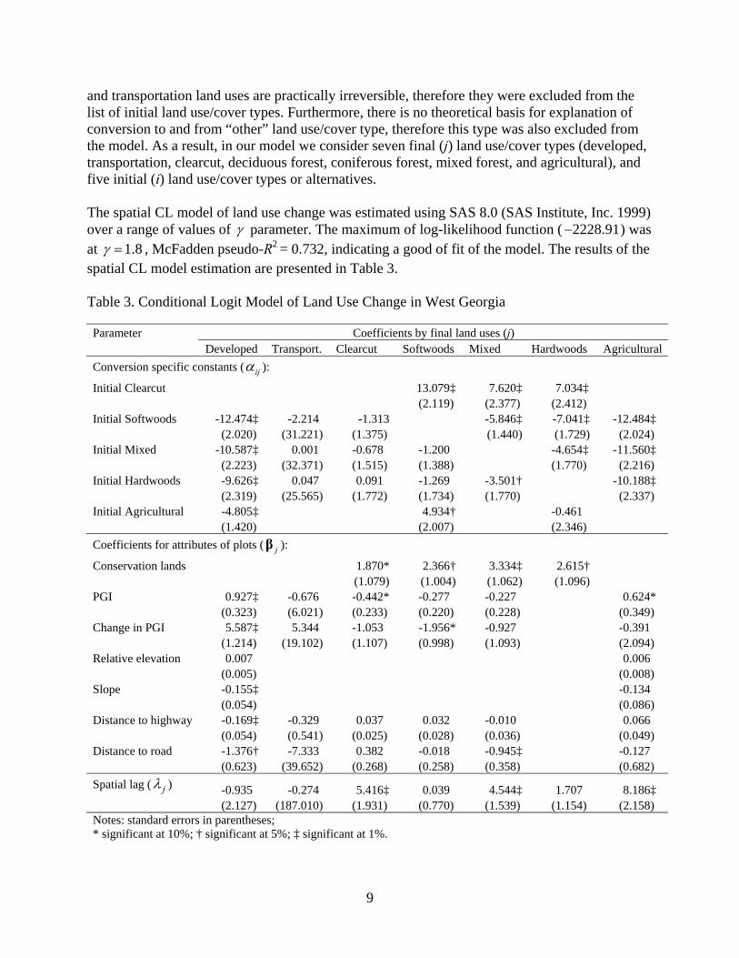
9

and transportation land uses are practically irreversible, therefore they were excluded from the list of initial land use/cover types. Furthermore, there is no theoretical basis for explanation of conversion to and from “other” land use/cover type, therefore this type was also excluded from the model. As a result, in our model we consider seven final (j) land use/cover types (developed, transportation, clearcut, deciduous forest, coniferous forest, mixed forest, and agricultural), and five initial (i) land use/cover types or alternatives. The spatial CL model of land use change was estimated using SAS 8.0 (SAS Institute, Inc. 1999) over a range of values of γ parameter. The maximum of log-likelihood function ( 2228.91− ) was at 1.8γ = , McFadden pseudo-R2 = 0.732, indicating a good of fit of the model. The results of the spatial CL model estimation are presented in Table 3. Table 3. Conditional Logit Model of Land Use Change in West Georgia Parameter Coefficients by final land uses (j) Developed Transport. Clearcut Softwoods Mixed Hardwoods Agricultural Conversion specific constants ( ijα ):

Initial Clearcut 13.079‡ 7.620‡ 7.034‡ (2.119) (2.377) (2.412) Initial Softwoods -12.474‡ -2.214 -1.313 -5.846‡ -7.041‡ -12.484‡ (2.020) (31.221) (1.375) (1.440) (1.729) (2.024) Initial Mixed -10.587‡ 0.001 -0.678 -1.200 -4.654‡ -11.560‡ (2.223) (32.371) (1.515) (1.388) (1.770) (2.216) Initial Hardwoods -9.626‡ 0.047 0.091 -1.269 -3.501† -10.188‡ (2.319) (25.565) (1.772) (1.734) (1.770) (2.337) Initial Agricultural -4.805‡ 4.934† -0.461 (1.420) (2.007) (2.346) Coefficients for attributes of plots ( jβ ):

Conservation lands 1.870* 2.366† 3.334‡ 2.615† (1.079) (1.004) (1.062) (1.096) PGI 0.927‡ -0.676 -0.442* -0.277 -0.227 0.624* (0.323) (6.021) (0.233) (0.220) (0.228) (0.349) Change in PGI 5.587‡ 5.344 -1.053 -1.956* -0.927 -0.391 (1.214) (19.102) (1.107) (0.998) (1.093) (2.094) Relative elevation 0.007 0.006 (0.005) (0.008) Slope -0.155‡ -0.134 (0.054) (0.086) Distance to highway -0.169‡ -0.329 0.037 0.032 -0.010 0.066 (0.054) (0.541) (0.025) (0.028) (0.036) (0.049) Distance to road -1.376† -7.333 0.382 -0.018 -0.945‡ -0.127 (0.623) (39.652) (0.268) (0.258) (0.358) (0.682) Spatial lag ( jλ ) -0.935 -0.274 5.416‡ 0.039 4.544‡ 1.707 8.186‡ (2.127) (187.010) (1.931) (0.770) (1.539) (1.154) (2.158) Notes: standard errors in parentheses; * significant at 10%; † significant at 5%; ‡ significant at 1%.

10

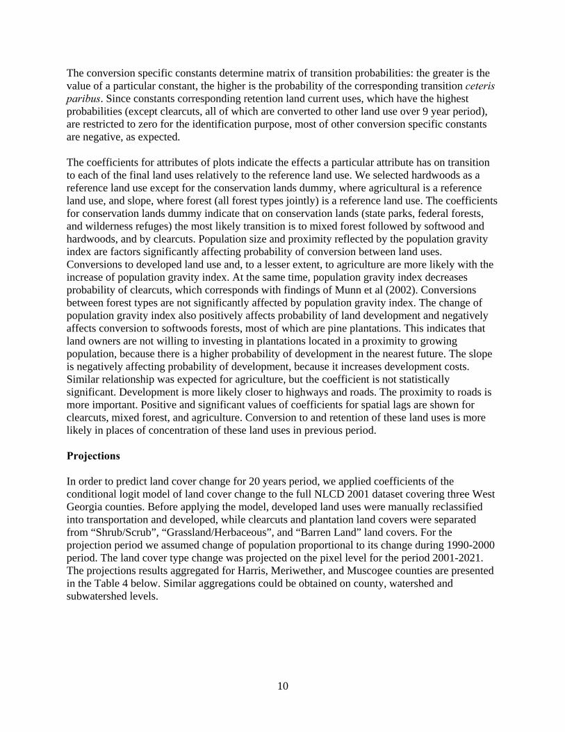
The conversion specific constants determine matrix of transition probabilities: the greater is the value of a particular constant, the higher is the probability of the corresponding transition ceteris paribus. Since constants corresponding retention land current uses, which have the highest probabilities (except clearcuts, all of which are converted to other land use over 9 year period), are restricted to zero for the identification purpose, most of other conversion specific constants are negative, as expected. The coefficients for attributes of plots indicate the effects a particular attribute has on transition to each of the final land uses relatively to the reference land use. We selected hardwoods as a reference land use except for the conservation lands dummy, where agricultural is a reference land use, and slope, where forest (all forest types jointly) is a reference land use. The coefficients for conservation lands dummy indicate that on conservation lands (state parks, federal forests, and wilderness refuges) the most likely transition is to mixed forest followed by softwood and hardwoods, and by clearcuts. Population size and proximity reflected by the population gravity index are factors significantly affecting probability of conversion between land uses. Conversions to developed land use and, to a lesser extent, to agriculture are more likely with the increase of population gravity index. At the same time, population gravity index decreases probability of clearcuts, which corresponds with findings of Munn et al (2002). Conversions between forest types are not significantly affected by population gravity index. The change of population gravity index also positively affects probability of land development and negatively affects conversion to softwoods forests, most of which are pine plantations. This indicates that land owners are not willing to investing in plantations located in a proximity to growing population, because there is a higher probability of development in the nearest future. The slope is negatively affecting probability of development, because it increases development costs. Similar relationship was expected for agriculture, but the coefficient is not statistically significant. Development is more likely closer to highways and roads. The proximity to roads is more important. Positive and significant values of coefficients for spatial lags are shown for clearcuts, mixed forest, and agriculture. Conversion to and retention of these land uses is more likely in places of concentration of these land uses in previous period. Projections In order to predict land cover change for 20 years period, we applied coefficients of the conditional logit model of land cover change to the full NLCD 2001 dataset covering three West Georgia counties. Before applying the model, developed land uses were manually reclassified into transportation and developed, while clearcuts and plantation land covers were separated from “Shrub/Scrub”, “Grassland/Herbaceous”, and “Barren Land” land covers. For the projection period we assumed change of population proportional to its change during 1990-2000 period. The land cover type change was projected on the pixel level for the period 2001-2021. The projections results aggregated for Harris, Meriwether, and Muscogee counties are presented in the Table 4 below. Similar aggregations could be obtained on county, watershed and subwatershed levels.

11

Table 4. Projections of land cover change for Harris, Meriwether, and Muscogee counties Land cover/use Harris Merriwether Muscogee Three counties 2001 2021 2001 2021 2001 2021 2001 2021 Developed 2.2% 6.6% 1.4% 3.4% 27.4% 33.7% 6.5% 10.2% Transportation 4.3% 4.7% 3.7% 3.8% 3.6% 3.7% 3.9% 4.2% Clearcut 4.4% 5.2% 5.2% 5.9% 0.4% 1.8% 4.0% 4.9% Deciduous forest 36.3% 31.7% 26.4% 22.4% 27.0% 23.4% 30.4% 26.3% Coniferous forest 33.9% 34.4% 34.4% 36.4% 18.0% 16.1% 31.2% 31.9% Mixed forest 0.7% 0.6% 0.8% 0.5% 7.1% 5.2% 1.9% 1.4% Riparian forest 3.4% 3.4% 6.4% 6.4% 4.5% 4.5% 4.9% 4.9% Agricultural 9.1% 7.7% 17.0% 16.6% 3.2% 2.7% 11.3% 10.5% Wetlands 0.0% 0.0% 0.0% 0.0% 0.2% 0.2% 0.0% 0.0% Water body 2.3% 2.3% 0.8% 0.8% 2.0% 2.0% 1.6% 1.6% Others 3.3% 3.3% 3.8% 3.8% 6.7% 6.7% 4.1% 4.1%

Literature Cited

Ahn, S., A. Plantinga, and R. Alig. 2000. Predicting future forestland area: A comparison of econometric approaches. Forest Science 46(3): 363-376.

Alig, R. J. and R. G. Healy. 1987. Urban and built-up land area changes in the United States: An

empirical investigation of determinants. Land Economics 63(3):215-226. Hardie, I. W., and P. J. Parks. 1997. Land Use with Heterogeneous Land Quality: An

Application of an Area-Base Model. American Journal of Agricultural Economics, 79(2):299–310.

Hunt, G. L. 2000. Alternative Nested Logit Model Structures and the Special Case of Partial

Degeneracy. Journal of Regional Science, 40(1):89–113. Kline, J. D., A. Moses, and R. J. Alig. 2001. Integrating Urbanization into Landscape-Level

Ecological Assessments. Ecosystems 4(1):3-18. Lubowski, R. N., A. J. Plantinga, and R. N. Stavins. 2006. Land-Use Change and Carbon Sinks:

Econometric Estimation of the Carbon Sequestration Supply Function. Journal of Environmental Economics and Management 51(2):135–152.

McFadden, D. 1973. Conditional Logit Analysis of Quantitative Choice Models. In Frontiers of

Econometrics, ed. P. Zarembka. New York: Academic Press. Mohammadian, A. and P. Kanaroglou (2003), Applications of Spatial Multinomial Logit Model

to Transportation Planning, Proceedings of the 10th International Conference on Travel Behaviour Research, Aug. 2003, Switzerland.

12

Munn, I. A., S. A. Barlow, D. L. Evans, and D. Cleaves. 2002. Urbanization’s impact on timber harvesting in the south central United States. Journal of Environmental Management, 64 (1), 65-76.

Nagubadi, V. R. and D. Zhang. 2005. Determinants of Timberland Use by Ownership and Forest

Type in Alabama and Georgia. Journal of Agricultural and Applied Economics 37(1):173–186.

Parks, P. J., and B. C. Murray. 1994. Land Attributes and Land Allocation: Nonindustrial Forest

Use in the Pacific Northwest. Forest Science 40(3):558-575. Plantinga, A. J., J. Buongiorno, and R. J. Alig. 1990. Determinants of Changes in Non-Industrial

Private Timberland Ownership in the United States. Journal of World Forest Resource Management 5:29-46.

SAS Institute, Inc. 1999. SAS/ETS User’s Guide, Version 8. SAS Institute Inc., Cary, NC, 1546

p. Stavins, R. N., and A. B. Jaffe. 1990. Unintended Impacts of Public Investments on Private

Decisions: The Depletion of Forested Wetlands. American Economic Review 80:337-352. Train, K. E. 2003. Discrete Choice Methods with Simulation. Cambridge University Press,

Cambridge, UK. 334 p. Zhang, D. and R.V. Nagubadi. 2005. Timberland Use in the Southern United States. Forest

Policy and Economics 7(3):721–731.

13

Impacts of Climate Change on Tennessee Forests

Donald G. Hodges1, 2, Virginia H. Dale3, and Jonah Fogel2 Abstract: Forests of Tennessee are diverse and have been affected by land use and management, nonnative species, outbreaks of native insects, and natural disturbances. The forests in Tennessee are likely to experience further changes in future decades due to climate change and related factors. This presentation describes a study initiated to assess the potential effect of these changes on the state’s forested ecosystems and on socio-economic variables due to the environmental changes. Specifically, a spatially explicit model of current and future forest conditions will be used to identify potential changes in forest characteristics such as forest type distribution, growth, and insect and disease outbreaks. Economic impacts of climate change will be assessed for changes in the forest products industry and forest-based recreation. The forest products effects will be estimated by determining the effects of the changes in composition and structure on the sustainability of the state’s forest industry, including estimates of changes in forest sector output and employment, yield, secondary impacts within related sectors, and the sustainability of the industry sector. Estimating the economic effects of climate change on recreational use will be accomplished primarily through projections of future climate scenarios and the potential effects on recreational demand and availability.

1 Corresponding author, dhodges2@utk.edu, (865) 974-2706 (v). 2 Oak Ridge National Laboratory, Environnemental Sciences Division. 3 Department of Forestry, Wildlife and Fisheries; The University of Tennessee; 274 Ellington Plant Sciences Bldg.; Knoxville, TN 37996-4563.

14

How Competitive Is the Wood Supply Chain in the U.S. South?

Jacek P. Siry1, 2, W. Dale Greene2, Thomas G. Harris, Jr.2, and Robert L. Izlar2 Abstract: Fiber is the largest component of cash manufacturing costs. As such, fiber availability and cost have large impacts on industrial profitability. We examine wood supply chains across the world’s major wood producing regions, including U.S. South, Canada, Brazil, Chile, Sweden, and Australia. We evaluate the effectiveness of particular systems based on information about their structure, stumpage costs, and delivered wood costs. The delivery process includes procuring, harvesting, and transporting fiber to the production’s facility woodyard and processing there. Using the linerboard sector as an example, we also examine the impact of using virgin fiber vs. recycled fiber on manufacturing costs. These regional comparisons are used to identify strategies that should be considered by the industry in the U.S. South for improving wood supply chain efficiency. A special emphasis will be placed on what policy makers and wood processing mills can do to improve the wood supply chain efficiency, both in terms of reducing costs and improving fiber availability, including policies associated with truck weight limits, scheduling, equipment, and contracting.

1 Corresponding author, jsiry@warnell.uga.edu, (706) 542-3060 (v), (706) 542-8356 (fax). 2 Center for Forest Business, Warnell School of Forestry and Natural Resources, University of Georgia, Athens, GA 30602-2152.

15

Is the Current Poor Market for Hardwood Lumber in North Carolina, Virginia, and West Virginia Temporary?

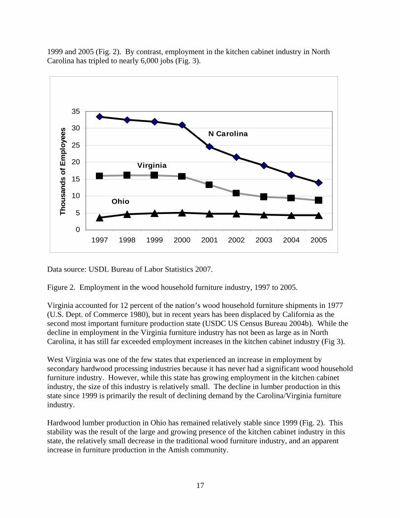
William G. Luppold1 and Matthew S. Bumgardner2 Abstract: Between 1999 and 2003 hardwood lumber production in the Central Appalachian region (North Carolina, Virginia, West Virginia, and Ohio) declined by 500 million board feet (mmbf) or 17 percent. In 2004 demand for hardwood lumber increased resulting in a 6 percent rise in eastern U.S. production. Eastern hardwood lumber production continued to increase in 2005 but production in North Carolina, West Virginia, and Virginia declined by 5.9, 4.3, and 4.1 percent, respectively. By contrast, production in Ohio increased by nearly 5 percent. Annual variation in lumber production in a particular state is not uncommon, but significant declines in lumber production in three adjacent states in the face of a stable national market may indicate a structural change. In this paper we examine how changes in demand and employment in secondary industries, demographics, timber inventory, and transportation costs influence hardwood lumber production in this region. Keywords: Hardwoods, demand, demographics Introduction In 1999 the Central Appalachian region (North Carolina, Virginia, West Virginia and Ohio) produced more than 2.9 billion board feet (bbf) of hardwood lumber (USDC US Census Bureau 2000). Between 1999 and 2003 lumber production in this region declined by more than 500 million board feet (mmbf) as overall eastern U.S. hardwood lumber production declined by 1.7 bbf (USDC US Census Bureau 2000, 2004a). In 2004 demand for hardwood lumber increased resulting in a 6 percent rise in eastern U.S. production (USDC US Census Bureau 2005). Eastern hardwood lumber production continued to increase in 2005 but production in North Carolina, West Virginia, and Virginia declined by 5.9, 4.3, and 4.1 percent respectively (Fig. 1). By contrast, production in Ohio increased nearly 5 percent (USDC US Census Bureau 2006). Annual variation in lumber production in a particular state or region can be the result of nonmarket factors, such as weather interacting with market factors. However, significant declines in lumber production in three adjacent states in the face of a stable national market may indicate a structural change. In this paper we examine how changes in demand and employment in the secondary industries have influenced lumber production in the central hardwood region since 1999. We also will examine how demographics, timber inventory, and transportation costs may interact with market forces to influence future competitiveness of this region.

1 Project Leader, USDA Forest Service, Northern Research Station, 241 Mercer Springs Road, Princeton, WV 24740, wluppold@fs.fed.us, (304) 431-2770 (v), (304) 431-2772 (fax). 2 Forest Products Technologist, USDA Forest Service, Northern Research Station, 241 Mercer Springs Road, Princeton, WV 24740, mbumgardner@fs.fed.us, (740) 368-0059 (v), (704) 368-0152 (fax).

16

300

400

500

600

700

800

900

1999 2000 2001 2002 2003 2004 2005

Mill

ions

of B

oard

Fee

t

Ohio

Virginia

W Virginia

N Carolina

Data source: USDL Bureau of Labor Statistics 2007.

Figure 1. Hardwood lumber production in Virginia, West Virginia, North Carolina and Ohio, 1999 to 2005. Demand and Employment in Secondary Processing Industries In 1999 the furniture industry consumed 2.6 bbf of lumber while the millwork, flooring, and kitchen cabinet industries consumed 1.3, 1.4, and 1.2 bbf, respectively (Hardwood Market Report 2007). In 2004 hardwood lumber consumption by the furniture industry was 1.3 bbf, a decline of 50 percent from 1999 levels. By contrast, consumption by the cabinet industry increased by 300 mmbf between 1999 and 2004. These shifts in consumption have made the hardwood lumber industry more dependent on home construction and remodeling (CR) industries with a growing volume of millwork and flooring being manufactured by smaller firms that serve local construction markets.

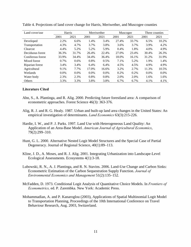
North Carolina has been the center of the U.S. wood household furniture industry since the mid 1950s and accounted for 28 percent of the nation’s wood household furniture shipments in 1977 (USDC Bureau of the Census 1980). While North Carolina remained the top furniture producer, production has declined to 11 percent of total furniture shipments (domestic production plus imports) in 2002 (USDC US Census Bureau 2004b, Akers 2006). Since 2002, domestic furniture production has continued to decline while imports have increased. These changes are reflected in the 19,000 jobs lost in North Carolina’s wood household furniture industry between

17

1999 and 2005 (Fig. 2). By contrast, employment in the kitchen cabinet industry in North Carolina has tripled to nearly 6,000 jobs (Fig. 3).

0

5

10

15

20

25

30

35

1997 1998 1999 2000 2001 2002 2003 2004 2005

Thou

sand

s of

Em

ploy

ees

Ohio

Virginia

N Carolina

Data source: USDL Bureau of Labor Statistics 2007.

Figure 2. Employment in the wood household furniture industry, 1997 to 2005.

Virginia accounted for 12 percent of the nation’s wood household furniture shipments in 1977 (U.S. Dept. of Commerce 1980), but in recent years has been displaced by California as the second most important furniture production state (USDC US Census Bureau 2004b). While the decline in employment in the Virginia furniture industry has not been as large as in North Carolina, it has still far exceeded employment increases in the kitchen cabinet industry (Fig 3). West Virginia was one of the few states that experienced an increase in employment by secondary hardwood processing industries because it has never had a significant wood household furniture industry. However, while this state has growing employment in the kitchen cabinet industry, the size of this industry is relatively small. The decline in lumber production in this state since 1999 is primarily the result of declining demand by the Carolina/Virginia furniture industry.

Hardwood lumber production in Ohio has remained relatively stable since 1999 (Fig. 2). This stability was the result of the large and growing presence of the kitchen cabinet industry in this state, the relatively small decrease in the traditional wood furniture industry, and an apparent increase in furniture production in the Amish community.

18

0

2000

4000

6000

8000

10000

1997 1998 1999 2000 2001 2002 2003 2004 2005

Thos

ands

of e

mpl

oyee

s

N Caorlina

Ohio

Virginia

Data source: USDL Bureau of Labor Statistics 2007.

Figure 3. Employment in the kitchen cabinet industry, 1997 to 2005.

Demographics Demographic factors (Table 1), including population, population growth, and income, are important because they are indicative of localized lumber demand by custom and semi custom CR product manufacturers. The rapid population growth in North Carolina and Virginia partly explains the rapid growth in kitchen cabinet production in these states. By contrast, Ohio and West Virginia had relatively low rates of population growth and the kitchen cabinet industry in these states is associated with large manufacturing facilities. Income and housing costs also vary considerably between and within states in the Central Appalachian region. Virginia has the highest per capita income, but this measure varies considerably when moving from the southwestern to the northeastern regions surrounding the District of Columbia (DC). While per capita income in North Carolina is considerably lower than Virginia, the lower cost of housing in the state and high population growth counters lower incomes. The combination of income and population factors makes Virginia and North Carolina viable future markets for custom and semi- custom CR producers. However, population growth results in expanding urbanization and decreased volume of land available for timbering (increased rural/urban interface). West Virginia has the lowest per capita income, but also large variations in income between the southwestern region and the eastern panhandle bordering the DC metropolitan area. While custom and semi-custom CR industries may be able to start up and survive in the eastern

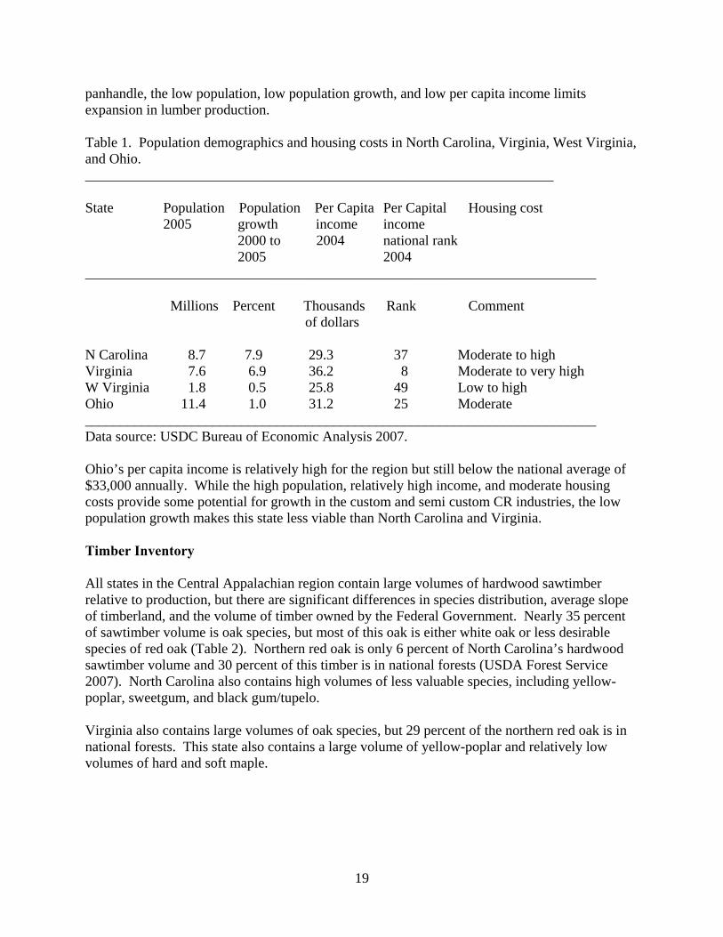
19

panhandle, the low population, low population growth, and low per capita income limits expansion in lumber production. Table 1. Population demographics and housing costs in North Carolina, Virginia, West Virginia, and Ohio. __________________________________________________________________ State Population Population Per Capita Per Capital Housing cost 2005 growth income income 2000 to 2004 national rank 2005 2004 ________________________________________________________________________ Millions Percent Thousands Rank Comment of dollars N Carolina 8.7 7.9 29.3 37 Moderate to high Virginia 7.6 6.9 36.2 8 Moderate to very high W Virginia 1.8 0.5 25.8 49 Low to high Ohio 11.4 1.0 31.2 25 Moderate ________________________________________________________________________ Data source: USDC Bureau of Economic Analysis 2007. Ohio’s per capita income is relatively high for the region but still below the national average of $33,000 annually. While the high population, relatively high income, and moderate housing costs provide some potential for growth in the custom and semi custom CR industries, the low population growth makes this state less viable than North Carolina and Virginia. Timber Inventory All states in the Central Appalachian region contain large volumes of hardwood sawtimber relative to production, but there are significant differences in species distribution, average slope of timberland, and the volume of timber owned by the Federal Government. Nearly 35 percent of sawtimber volume is oak species, but most of this oak is either white oak or less desirable species of red oak (Table 2). Northern red oak is only 6 percent of North Carolina’s hardwood sawtimber volume and 30 percent of this timber is in national forests (USDA Forest Service 2007). North Carolina also contains high volumes of less valuable species, including yellow-poplar, sweetgum, and black gum/tupelo. Virginia also contains large volumes of oak species, but 29 percent of the northern red oak is in national forests. This state also contains a large volume of yellow-poplar and relatively low volumes of hard and soft maple.

20

Table 2. Timber volume, average slope, composition for major species groups and percentage of timber contained in national forests. ________________________________________________________________________ State Timber Average Red White Gums Yellow Hard Soft National volume slope oaks oaks -poplar maple maple forest (bbf) (%) (%) (%) (%) (%) (%) (%) (%) ________________________________________________________________________ N Carolina 63.7 23.0 17.5 17.3 16.7 26.8 0.6 6.7 11.3 Virginia 68.5 25.3 21.3 24.1 6.1 27.7 1.2 4.5 12.7 W. Virginia 69.5 37.2 20.6 19.1 2.8 20.4 6.6 6.3 8.9 Ohio 39.7 21.8 13.1 14.3 0.5 13.3 7.5 9.2 3.6 ________________________________________________________________________ Data source: USDA Forest Service 2007 Nearly half of the red oak in West Virginia is northern red or other preferred red oak species. While this state also contains high volumes of yellow-poplar, it also contains several industries that utilize this species, including hardwood plywood, laminated veneer lumber, and oriented strand board. West Virginia contains relatively high volumes of hard and soft maple and low volumes of gum species. However, much of the timber in this state is on steep slopes and is expensive to access and transport. Ohio has the most diversified timber resource and arguably the most valuable resource. Most of the state’s oak resource is select white and red oak species. Ohio also contains relatively high volumes of hard and soft maple, virtually no gum species, and relatively low volumes of yellow-poplar. Less than 4 percent of the timber in Ohio is in national forests.

Transportation Costs The cost of harvesting and transporting logs and lumber has been escalating because of increased fuel costs. When fuel costs are high, mills close to secondary processors have a comparative advantage to mills that are more remote. Higher fuel costs also might benefit custom and semi-custom CR operations that are close to the final customer. West Virginia will be most affected by high fuel costs because of the difficultly of accessing timber, the distance to secondary processors outside the state, and the relatively small secondary processing industry within the state. State Competitiveness The current state of the furniture industry and cooling housing market in the United States translates into an uncertain short-term outlook for the hardwood lumber industry. A potential bright point is that people will continue to renovate their own homes thus driving the remodeling portion of the construction industry. However, given current trends in demand and energy costs, some states will have a comparative advantage (Table 3).

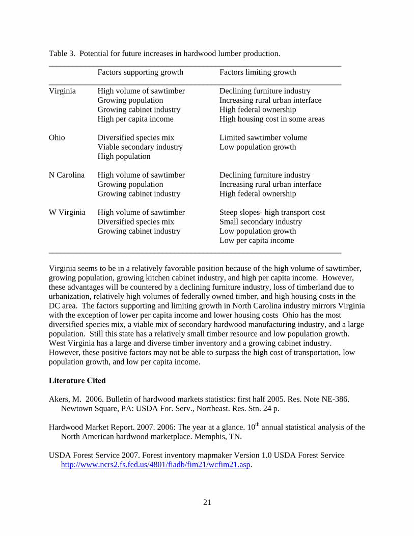
21

Table 3. Potential for future increases in hardwood lumber production. ________________________________________________________________________ Factors supporting growth Factors limiting growth ________________________________________________________________________ Virginia High volume of sawtimber Declining furniture industry

Growing population Increasing rural urban interface Growing cabinet industry High federal ownership

High per capita income High housing cost in some areas

Ohio Diversified species mix Limited sawtimber volume Viable secondary industry Low population growth

High population

N Carolina High volume of sawtimber Declining furniture industry Growing population Increasing rural urban interface Growing cabinet industry High federal ownership W Virginia High volume of sawtimber Steep slopes- high transport cost Diversified species mix Small secondary industry Growing cabinet industry Low population growth Low per capita income ________________________________________________________________________ Virginia seems to be in a relatively favorable position because of the high volume of sawtimber, growing population, growing kitchen cabinet industry, and high per capita income. However, these advantages will be countered by a declining furniture industry, loss of timberland due to urbanization, relatively high volumes of federally owned timber, and high housing costs in the DC area. The factors supporting and limiting growth in North Carolina industry mirrors Virginia with the exception of lower per capita income and lower housing costs Ohio has the most diversified species mix, a viable mix of secondary hardwood manufacturing industry, and a large population. Still this state has a relatively small timber resource and low population growth. West Virginia has a large and diverse timber inventory and a growing cabinet industry. However, these positive factors may not be able to surpass the high cost of transportation, low population growth, and low per capita income. Literature Cited Akers, M. 2006. Bulletin of hardwood markets statistics: first half 2005. Res. Note NE-386.

Newtown Square, PA: USDA For. Serv., Northeast. Res. Stn. 24 p. Hardwood Market Report. 2007. 2006: The year at a glance. 10th annual statistical analysis of the

North American hardwood marketplace. Memphis, TN. USDA Forest Service 2007. Forest inventory mapmaker Version 1.0 USDA Forest Service

http://www.ncrs2.fs.fed.us/4801/fiadb/fim21/wcfim21.asp.

22

USDC Bureau of Economic Analysis 2007. Regional economic accounts. http://www.bea.gov/bea/regional/bearfacts/stateaction.cfm?fips=54000&yearin=2005.

USDC Bureau of the Census. 1980. 1977 Census of manufactures, household furniture. MC77-I-

25A USDC Bureau of the Census, Washington, D.C. USDC US Census Bureau 2000. Current industrial reports; lumber production and mill stocks:

1999. MA321T(99)-1 USDC US Census Bureau, Washington, D.C. USDC US Census Bureau 2004a. Current industrial reports; lumber production and mill stocks:

2003. MA321T(03)-1 USDC US Census Bureau, Washington, D.C. USDC US Census Bureau 2004b. 2002 Economic census nonupholstered wood household

furniture manufacturing EC02-31I-337122 (RV) USDC Bureau of the Census, Washington, D.C.

USDC US Census Bureau 2005. Current industrial reports; lumber production and mill stocks:

2004. MA321T(04)-1 USDC US Census Bureau, Washington, D.C. USDC US Census Bureau 2006. Current industrial reports; lumber production and mill stocks:

2005. MA321T(05)-1 USDC US Census Bureau, Washington, D.C. USDL Bureau of Labor Statistics 2007. Series report. http://data.bls.gov/cgi-bin/srgate.

23

An Econometric Analysis of Pine Pulpwood Market in the Southern US

Xianchun Liao1 and Yaoqi Zhang2

Abstract: This paper examines the determinants of pine pulpwood supply and demand in the southern US using annual data from 1950 to 2002. A structural simultaneous system of equations (SSE) model is used to estimate short-run price elasticities with three-stage least squares (3SLS) regression techniques. The results show that price elasticities of supply of and demand for pine pulpwood are relatively small, but similar to those reported for the US South. The results also show that the cross elasticity with pine sawtimber is significantly positive at the 5% level, but very small in magnitude at 0.11, which is consistent with the previous finding. The significant substitution between pulpwood stumpage and energy use was found with elasticity of -0.35. Keywords: Energy use, pine pulpwood market, simultaneous system of equations, market equilibrium Introduction More than 83% of softwood pulpwood production in the United States came from the South (Howard 2003, p.6) and some 72% of timberland in the South was owned by nonindustrial private forest (NIPF) landowners in 2002 (Smith et al. 2004). These landowners supply stumpage to loggers or wood-dealers whereas paper processors produce final product combining processing inputs (such as capital and labor) with the log materials delivered by the loggers or wood-dealers. In 2004, 89 southern pulpmills were operating and pulping capacity of 125 thousand tons per day accounts for more than 70 percent of the Nation’s total pulping capacity (Johnson and Steppleton 2004, p.7). Understanding the characteristics of the stumpage market has been an important aspect in modeling exercises or forecast efforts, public policy and management plan. For example, Adams and Haynes (1980), Newman (1987), and Carter (1992) emphasize timber supply and demand issues and give insights into the determinants of quantity supplied and demanded, and price. Another example is supply and demand elasticities of stumpage play significant roles in measuring welfare impacts (e.g., Li and Zhang 2006). Modeling the stumpage market is also useful for assessing the effects of cost-sharing and technical assistance on reforestation (e.g., Royer 1987, Hyberg and Holthausen 1989, Zhang and Pearse 1996, and Zhang and Flick 2001).

Timber market models are extensively used to estimate short-run elasticity for forest landowners (e.g., Brännlund et al. 1985, Newman 1987, Carter 1992, and Polyakov et al. 2005); however, 1 Research Associate, School of Forestry and Wildlife Sciences, Auburn University, AL 36849, liaoxia@auburn.edu, (334) 844 8042 (v), (334) 844-1084 (fax). 2 Assistant Professor, School of Forestry and Wildlife Sciences, Auburn University, AL 36849, Yaoqi.Zhang@auburn.edu, (334) 844-1041 (v), (334) 844-1084 (fax).

24

few studies consider energy use in pulpwood market in the US South (Liao 2007). Most of previous studies have small samples covering only 20-30 annual observations. The small observations with time series data might cause the coefficients of a simultaneous system of equations (SSE) to be sensitive to its specification and even inconsistent (Wooldridge 2000). In addition, most of previous studies pay little attention to energy used in the production of paper and allied products. Energy use among US pulp, paper, and paperboard mills accounts for about 12% of all energy used in the domestic manufacturing sector and shares production cost by 13% within the paper mills (NAF 2002, Brown and Zhang 2005). Moreover, most of previous studies often ignore recycled paper, which is an increasingly significant input for environment reasons. The wastepaper utilization accounts for 42% for newsprint, 10% for printing/writing paper, 60% for tissue paper, and 15% for packaging paper, respectively (Brown and Zhang 2005).

Therefore, this study is to estimate pine pulpwood supply and demand using structural SSE approach in the Southern US because this approach has its own advantages. First, a structural SSE is a partial equilibrium model based on economic theory. Variable choices make economic sense. Second, an advantage of a structural SSE over non structural vector autoregression (VAR) model is that it estimates multiple equations simultaneously and enables us to obtain the price elasticities in the short run.

The paper is organized as follows. First, the theoretical models of pine pulpwood stumpage supply and demand are presented. Then, the data sources are presented and the empirical estimation using three-stage least squares (3SLS) follows. Next, the regression results are interpreted. The study ends with summary and conclusion.

Theoretical Framework Demand for stumpage derives from its use as a raw material in the production of paper and paperboard products. Paper and paperboard firms purchase the stumpage in the market along with other inputs (e.g. labor, capital) to provide their particular output. Following the early authors’ framework (Newman 1987, Brown and Zhang 2005), the production function for a competitive firm i is assumed to be twice continuously differentiable. Thus,

),,,,(Qit itititititi DWEKLq= (1) where i = 1,..., N; t = annual observations (1950, …, 2002) for pulpwood; Qit is the quantity of paper and paperboard production by firm i in period t; and Lit, Kit, Eit, Wit,and Dit are the quantities of labor, capital, energy, wastepaper, and raw material that firm i uses in period t. The paper and paperboard products trade in national markets, and as such, the final good price (FP) is exogenous to the region. The profit function for firm i in period t is:

itititititititititititititititit DPPWrEeKiLwDEKLqFP −−−−−= ),,,(Max itπ (2) where wit, iit, eit, rit, and PPit are for the particular industry, the respective prices of labor, capital, energy, recycled paper and pine pulpwood stumpage.

25

Applying Hotelling’s lemma, the firm’s derived demand for stumpage in period t is a function of market price and the prices of all inputs in production. The demand function for stumpage Di is found by taking the first derivative of the profit function (Varian 1978, p.31). Thus,

),,,,,(/????

it−+

=∂∂ itititititititit PPreiwFPDPPπ (3)

where the signs below the variables represent the expected effects on stumpage demand given an increase in output price or stumpage input costs. The signs for the wage, capital, and energy are uncertain because they depend on whether stumpage is a technical complement or substitute with other inputs (Newman 1987). If all the firms in the southern region have the same production function and face the same input prices, the regional stumpage demand equation can be obtained by aggregating the N individual firm’s demand functions. Thus,

),,,,,()PP,r,e,i,w,(FPD1

ttttttt itititititit

N

iit PPreiwFPD∑

=

= (4)

This equation serves as the theoretical model for the analysis. The aggregated roundwood supply is assumed to be a function of the received price for roundwood and the harvesting costs suggested by Newman (1987). There are several reasons for the assumption. First, the differentiated ownership and management structure of forestland in the South complicates the aggregation of individual roundwood supply functions as was done by Brännlund et al. (1985) and Kuuluvainen (1986). If owner-specific data is available, a complete production function specification is possible, though still problematic (Brännlund et al. 1985). Second, numerous factors influence the individuals output of roundwood such as multiple potential outputs (sawlog, pulp and paper log, poles), long delay between production decisions and the presence of government regulation. These concerns recommend hypothesizing a simplified supply function that still accounts for the returns and costs from forest management (Newman 1987). The amount of standing softwood pulpwood inventory serves as an inverse proxy for harvesting costs. Pine sawtimber stumpage might influence the output of pine pulpwood suggested by Newman (1987). Thus, the supply specification is as the following:

),,(S?

jt++

= jtjtjtj vSPPPS (5)

The own price for the pulpwood supply function is positive while the sign on sawtimber price is uncertain. Timber inventory has a positive effect on the output because the marginal harvesting costs decrease as inventory increases. If all the forest owners in the region maintain the same production, the regional stumpage supply specification can be found by aggregating the N individual forest owner’s production functions. Thus,

),,(),,(1

jtjtjt

N

jjttttt vSPPPSvSPPPS ∑

=

= (6)

26

The equation serves the theoretic model for this analysis and shows that the stumpage supply of pine pulpwood depends on owen price, sawtimber price, and inventory. Finally, a market clearing assumes that the quantity of supply and demand should be equal. Thus:

),,,,,(),,( ttttttttttt PPreiwFPDvSPPPS = (7) Keep in mind, transportation costs are assumed a relatively constant fraction of the stumpage price and do not affect the short-run supply and demand in the region. The SSE model satisfies the order condition for identification because there are two endogenous variables (Dem and PP) and more than two excluded exogenous variables (PPI, w, i, r, e, t) in the demand equation. Likewise, there are two endogenous variables (SUP and PP) and more than two excluded exogenous variables (V and SP) in the supply equation. The SSE model was estimated with three-stage least squares (3SLS) because it is consistent and asymptotically more efficient than two-stage least squares (2SLS) in overidentified systems (Wooldridge 2000, p516). It is clear that ordinary least squares (OLS) is inconsistent for the SSE model. In the empirical estimation, EViews 5.1 is used. Data Sources

Data sources are described in Table 1. Softwood stumpage is the total quantity of pine pulpwood of the 13 southern states covered by the Southeastern and Southern Forest Experiment Stations of the USDA Forest Service. The softwood roundwood imports from and exports to the region are ignored because both are relatively small quantities. The average volume-weighted stumpage price of southern pine pulpwood for 1977-2002 is from Timber Mart-South and for 1950-1976 from Ulrich (1989). Likewise, the average volume-weighted stumpage price of southern pine sawtimber for 1977-2002 is from Timber Mart-South and for 1950-1976 from Ulrich (1989). The US bank prime loan is used as the opportunity cost of capital (www.federalreserve.gov/releases/h15/data). The producer price index of the paper and allied products is employed as the final product price from the Bureau of Labor and Statistics (BLS). Wage rate is from the BLS. The producer price index of waste or recycled paper is also obtained from BLS, which serves as a proxy for the wastepaper price. Annual data for electricity is also taken from the BLS index for industrial electric power. Standing timber inventory for 1950-1985 is from Adams (1988) and for 1986-2002 from Smith et al. (2004). The missing data is found based on the formula from Newman (1987). The formula is specified as the following:

)([ **1 SSGvv ttt −−+= − , where G* is the average annual net growth between survey years and

S* is the average stumpage production between survey years. All data are annual and the time series cover the period from 1950 to 2002 (53 observations). The deflator is the Producer Price Index used for all prices from the US Department of Commerce (1982=100) and the Consumer Price Index is used for wage rate from the US BLS (1982=100).

27

Empirical Results

Both linear and log-linear forms are explored to estimate the SSE model. The log-log form results are reported here because it outperforms better than linear form in terms of coefficient significant. In addition, the logarithmic transformation can partly overcome exponential trends of these time series and the coefficients have an interpretation as elasticity. The White’s tests indicate that no heteroscedasticity is present in the SSE model. Following the procedure from a special case of the White test (Wooldridge 2000, p. 260), we obtain the F-values (2.12 for the demand equations and 0.53 for the supply equations). Both of them are less than the value of F2,50 distribution at the 5% level (F2,50 =3.19), indicating we fail to reject homoskedasticity. The low values for the Durbin Watson (DW) statistic in the SSE model reveal a problem of serial correlation in the system. However, the statistical package in this study cannot correct the serial correlation for the system equations (Newman 1987). Alternatively, one treatment is to calculate serial correlation-robust standard error, while keeping other results of the SSE model, following the framework of Newey-West (Wooldridge, 2000, p.395). However, the SC-robust standard errors may be poorly behaved when there is substantial serial correction and the sample size is small. In addition, the OLS used in the system can be very inefficient. Table 2 presents the regression results for pine pulpwood supply and demand. Overall, the explanatory variables significantly explain the dependent variables because the R2 values are high. The coefficients have the expected sign and most of them are significant.

On the demand side, the own price elasticity is significantly negative at the 5% level, but very inelastic with an estimated value of 0.22. On contrary, the final good price (paper and allied products) is significantly positive with an elasticity of 0.37, unlike previous studies where the final good price is not significantly different from 0. After a careful examination, we find that some degree of complements exists between stumpage and capital, while stumpage and energy are technical substitute. Both of these coefficients are significant at the 5% level. However, neither labor shows significantly positive relationship with stumpage, or recycled paper shows significantly negative relationship with stumpage.

On the supply side, the own price elasticity is significantly positive at the 1% level, but very inelastic with an estimated value of 0.35. The inventory elasticity is significantly positive at the 1% level and close to 1, which means that a 10% increase in the growing stock tends to increase pulpwood production by 8.9 %. The cross elasticity with pine sawtimber is significantly positive at the 5% level, but very small in magnitude at 0.11.

The estimated elasticities in this study can only be partially compared with existing values in the literature because of difference in methodology, data sources and regional focus. Table 3 compares price and inventory elasticities from this study and other studies for the US South. The price elasticities of softwood pulpwood demand and supply were found to be relatively small in this study, but similar to those reported for the US South (e.g. Newman 1987, Carter 1992, and Polyakov 2005).

28

Concluding Remarks The primary objective of the paper is to provide an up-to-date econometric analysis of pine pulpwood supply and demand in the South. To that end, a structural SSE model is developed and three-stage least squares regression techniques were used for that model. The results show that price elasticities of supply of and demand for pine pulpwood are relatively small, but similar to those reported for the US South (e.g. Newman 1987, Carter 1992). The results also show that the cross elasticity with pine sawtimber is significantly positive at the 5% level, but very small in magnitude at 0.11, which is consistent with the finding by Newman (1987). Finally, the significantly substitution between pulpwood stumpage and energy was found with elasticity -0.35. The study makes two contributions to the U.S. timber supply and demand literature. First, a five-factor demand specification for pine pulpwood stumpage is employed, while previous studies often ignore recycled paper and energy uses. Second, on the supply side, the complementary role of sawtimber in pulpwood production for the US South is found to be similar in Sweden (Johansson and Löfgren 1985), while it does not hold for Texas (Carter 1992).

The finding in this study may have implications on paper industry processors, landowners, and public policymakers. Paper industry processors should aware that any policy change in increasing capital investment may result in demand increase for pulpwood. Landowners who pursue profits from pulpwood production may consider the complementary role of sawtimber because sawtimber generates more revenue than pulpwood. The apparent substitution between wood and energy use produces a possible dilemma for environmental policymakers. If a hypothetical environmental tax is imposed on industrial electricity use, it may increase natural resource consumption. Further research is needed to examine pine pulpwood production by different ownerships so that a complete production function could be specified. In addition, the long-run relationship among the variables could be examined.

Literature Cited Adams, D.M., K.C. Jackson, and R.W. Haynes. 1988. Production, consumption and prices of

softwood products in North America: Regional time series data, 1950–1985. Resource Bull. PNW-RB-151, USDA For. Serv. Pacific Northwest Res. Stn., Portland, OR. 49 p.

Adams, D.M., and R.W. Haynes. 1980. The 1980 softwood timber market assessment model:

Structure, projections, and policy simulations. For. Sci. Monograph 22:64. 64 p. Brännlund, R., P.O. Johansson, and K.G. Löfgren. 1985. An economic analysis of aggregate

sawtimber and pulpwood supply in Sweden. For. Sci. 31: 595-606. Brown. R., and D. Zhang. 2005. Estimating supply elasticity for disaggregated paper products: a

primal approach. For. Sci. 51(6):570-577. Bureau of Labor Statistics. 2006. The producer price index (PPI). http://www.bls.gov/ppi.

29

Carter, D.R. 1992. Effects of supply and demand determinants on pulpwood stumpage quantity and price in Texas. For. Sci. 38(3):652-660.

Enders, W. 1995. Applied econometric time series. John Wiley & Sons, Inc., New York. 433 p. EViews. 2004. Eviews User’s Manual. Quantitative Micro Software. Johnson, T.G., and C.D. Steppleton. 2004. Southern Pulpwood Production, 2004. Resource

Bulletin SRS-111. USDA FS Southern Research Stattion, Asheville, NC. 39 p. Johansson, P.O. and K.G. Löfgren. 1985. The Economics of Forestry and Natural Resources.

Basil Blackwell, Oxford. 300p. Howard, J.L. 2003. U.S. Timber Production, Trade, Consumption, and Price Statistics 1965-

2002. Gen. Tech. Rep. FPL-RP-615. USDA Forest Service, Madison, WI. 90 p. Hyberg, B.T., and D.M. Holthausen. 1989. The behavior of nonindustrial private forest

landowners. Can. J. For. Res. 19:1014 –1023. Kuuluvainen, J. An econometric analysis of the sawlog market in Finland. J. World For. Res.

Manage. 2: 1-19. Liao, X. 2007. Essays of Forestry Investments in the US and Stumpage Market in the Southern

US. PhD Dissertation. Auburn University. 98 p. Li, Y., and D. Zhang. 2006. incidence of the 1996 U.S.-Canada softwood lumber agreement

among landowners, loggers, and lumber manufacturers in the U.S. South. For. Sci. 52(4): 422-431.

NAF (North American Fact Book). 2002. Ed. G. Rudder, G. (Ed.). Paperloop, San Francisco.

435 p. Newman, D.H. 1987. An econometric analysis of the southern softwood stumpage market: 1950-

1980. For. Sci. 33(4): 932-945. Polyakov, M., L. Teeter, and J.D. Jackson. 2005. An Econometric analysis of Alabama's

pulpwood market. For. Prod. J. 55: 4-14. Royer, J.P. 1987. Determinants of reforestation behavior among southern landowners. For. Sci.

33(3):654–667. Smith, W.B., P.D. Miles, J.S. Vissage, and S.A. Pugh. 2004. Forest resources of the United

States, 2002. U.S. Department of Agriculture, Forest Service, North Central Research Station, St. Paul, MN. Gen. Tech. Rep. NC-241. 137 p.

Timber Mart-South. 1977-2001. Highlands NC: Timber Mart-South, Inc.

30

Ulrich, A.H. 1989. U.S. Timber Production, Trade, Consumption, and Price Statistics 1950-87. Forest Service, U.S. Department of Agriculture.

Varian, H.R. 1978. Microeconomic analysis. New York, W.W. Norton. 284 p. Wooldridge, J.M. 2000. Introductory econometrics: A modern approach. South-Western College

Publishing, Boston, MA. 824 p. Zhang, D., and P.H. Pearse. 1996. Differences in silvicultural investment under various types of

forest tenure in British Columbia. For. Sci. 42(4): 442-449. Zhang, D., and W.A. Flick. 2001. Sticks, carrots, and reforestation investment. Land Econ.

77(3): 443-456.

31

Table 1. Data description and sources.

Variable (Abbreviation) Measurement Source

Pine pulpwood demand (DEM) Million cord Southern Forest Experiment Station

Pine pulpwood supply (SUP) Million cord Southern Forest Experiment Station

Stumpage price of pine pulpwood (PP) US$/Standard cord 1977-1999 from Timber Mart-South,

1950-1976 from Ulrich (1989) Stumpage price of pine sawtimber (SP)

US$/Thousand board feet (Scribner)

1977-1999 from Timber Mart-South, 1950-1976 from Ulrich (1989)

Paper and allied products (FP) Index (1982=100) US Bureau of Labor Statistics

Inventory (v) Million cubic feet 1950-1985 from Adams et al (1988), 1986-2002 from Smith et al. (2002)

Wage rates (w) U.S.$ per hour US Bureau of Labor Statistics Capital cost (i) % US Federal Reserve Recycled paper (r) Index (1982=100) US Bureau of Labor Statistics Energy (e) Index (1982=100) US Bureau of Labor Statistics Technical change (t) Integer From 1 for 1950 to 53 for 2002 U.S. Consumer Price Index (CPI) 1982=100 US Bureau of Labor Statistics

U.S. Producer Price Index (PPI) 1982=100 US Bureau of Labor Statistics

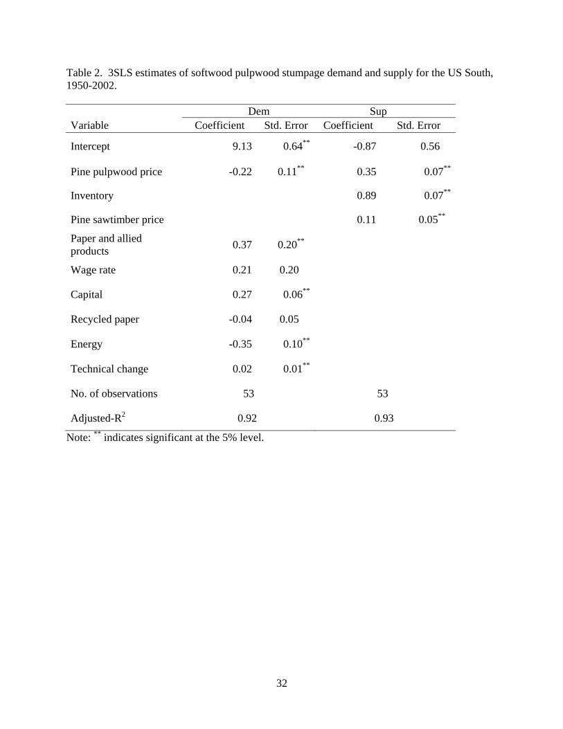
32

Table 2. 3SLS estimates of softwood pulpwood stumpage demand and supply for the US South, 1950-2002. Dem Sup Variable Coefficient Std. Error Coefficient Std. Error

Intercept 9.13 0.64** -0.87 0.56

Pine pulpwood price -0.22 0.11** 0.35 0.07**

Inventory 0.89 0.07**

Pine sawtimber price 0.11 0.05**

Paper and allied products 0.37 0.20**

Wage rate 0.21 0.20

Capital 0.27 0.06**

Recycled paper -0.04 0.05

Energy -0.35 0.10**

Technical change 0.02 0.01**

No. of observations 53 53

Adjusted-R2 0.92 0.93

Note: ** indicates significant at the 5% level.

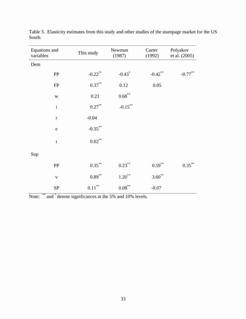
33

Table 3. Elasticity estimates from this study and other studies of the stumpage market for the US South. Equations and variables This study Newman

(1987) Carter (1992)

Polyakov et al. (2005)

Dem

PP -0.22** -0.43* -0.42** -0.77**

FP 0.37** 0.12 0.05

w 0.21 0.68**

i 0.27** -0.15**

r -0.04

e -0.35**

t 0.02**

Sup

PP 0.35** 0.23** 0.59** 0.35**

v 0.89** 1.20** 3.60**

SP 0.11** 0.08** -0.07

Note: ** and * denote significances at the 5% and 10% levels.

34

A Review of Econometric Models for Softwood Lumber

Nianfu Song and Sun Joseph Chang1

Abstract: Past softwood lumber models have estimated price elasticities of the U.S. lumber demand ranging from -0.07 (Adams and Haynes, 1996) to -1.15 (Adams et al., 1992) with -0.17 obtained by Adams et al.(1986) used the most often. Some of the studies estimated both long-run and short-run elasticities while others do not specify if their results are for the long-run or short-run. In terms of data frequency, some of the models were estimated with annual data; others with quarterly data or monthly data. This paper will review published lumber models from 1980 and group them into long-run or short-run categories based on time series theories. Nonstationarity and endogeneity in these models will be reviewed. The implication of the estimated elasticities will be discussed according to the model forms and frequencies of their data used. The magnitude of the elasticties will be discussed according to the review of the models.

1 Respectively, Graduate Research Assistant and Professor, Louisiana State University, nsong123@yahoo.com (N. Song).

35

Measuring Oligopsony and Oligopoly Power in the U.S. Paper Industry

Bin Mei and Changyou Sun1

Abstract: The U.S. paper industry has been increasingly concentrated ever since the 1950s. Such an industry structure may be suspected of imperfect competition. This study applied the new empirical industrial organization (NEIO) approach to examine the market power in the U.S. paper industry. Beginning with the identification of the production function, the econometric analysis was based on the formulation and estimation of a simultaneous-equation model consisting of a production function, first-order conditions for factor employment, and two conjectural elasticities indicating the industry’s oligopsony and oligopoly equilibria. By employing annual data from 1955 to 2003, the above system of equations was estimated by Generalized Method of Moments (GMM) procedure. The analysis indicated the presence of oligopsony power but no evidence of oligopoly power over the sample period.

Keywords: Conjectural elasticity, GMM, market power, NEIO Introduction The paper sector (NAICS 32-SIC 26) has been the largest among the lumber, furniture, and paper sectors in the U.S. forest products industry. According to the latest Annual Survey of Manufacturing in 2005, the value of shipments for paper manufacturing reached $163 billion or a 45% share of the total forest products output (U.S. Bureau of Census 2005). Thus, the paper sector has played a vital role in the U.S. forest products industry. However, spatial factors such as the cost of transporting products between sellers and buyers can mitigate the forces necessary to support perfect competition (Murray 1995a). This is particularly true in markets for agricultural and forest products. For example, timber and logs are bulky and land-intensive in nature, thus leading to high logging service fees. In fact, the share of harvesting margin, which is defined as the difference between the delivered log price and the stumpage price over the delivered log price, has been as high as around 60% in Mississippi for the last 30 years (Guo et al. March 2007). In addition, the high concentration in the paper industry has also aroused concern about its market power. In 2002, the CR4, as measured by the share of value of shipments accounted by the largest four companies in the industry, has reached 49% (U.S. Bureau of Census 2006), and actually the CR4 for the U.S paper industry has been ever increasing since 1954 from around 18% (Economic Census, various years). Such a structurally asymmetric industry, i.e., relative few timber processors in contrast to a large number of forest landowners and paper products consumers, may result in imperfect competition in both the pulpwood input market and the paper products output market. This situation has even

1 The authors are, respectively, Graduate Research Assistant and Assistant Professor, Department of Forestry, Mississippi State University, Box 9681, Mississippi State, MS 39762, csun@cfr.msstate.edu (C. Sun), (662) 325-7271 (v), (662) 325-8726 (fax). The authors thank Drs. Robert K. Grala, Anwar Hussain and Ian A. Munn for comments on the manuscript.

36

been aggravated by those huge mergers and acquisitions (M&As) in recent decades. Therefore, both oligopsony and oligopoly power can be suspected in the U.S paper industry. By employing annual data from 1955 to 2003, this study examined the market power in both the pulpwood input and paper products output markets in the U.S. paper industry simultaneously. Results from this study will be helpful in understanding the market behavior of the U.S. paper industry. Background and Previous Studies Market power possessed by industrial firms has been an issue of great interest in the past years. Geroski (1988), Bresnahan (1989), Kadiyali, et al. (2001) and Digal and Ahmadi-Esfahani (2002) provided excellent reviews of empirical approaches in the market power literature. Overall, there have been two major methods, i.e., the structure-conduct-performance paradigm (SCPP) approach and the new empirical industrial organization (NEIO) approach. Prior to 1980’s, the dominant approach was the SCPP. Based on the assumption that the level of competition could be implied by an industry’s structural features, the SCPP approach tried to establish a direct link from industry structure to conduct. Yet, the SCPP approach was criticized later because the relationship between industry structure and conducts was not unambiguously predicted by the theory of imperfect competition, and high concentration in an industry did not necessarily imply noncompetitive behavior (Ronnila and Toppinen 2000). To study the existence of market power more rigorously, researchers have gradually turned to the NEIO approach. One prominent component of the NEIO approach is to estimate the conjectural elasticities, also defined as market conduct parameters. The conjectural elasticities measure the overall market reaction to an individual firm’s change in input demand and output supply. A review of the NEIO studies revealed that most of the attention in the NEIO literature has been paid to the imperfect competition in either the input or output market. Research that considered both markets simultaneously has been limited. The exceptions are those several studies in the U.S. food processing industry (Schroeter 1988; Azzam and Pagoulatos 1990; Wann and Sexton 1992; Alston et al. 1997; Sexton 2000). Models that only examined oligopsony or oligopoly power ran the risk of understating the extent of the market power distortion or erroneously attributing distortions to the wrong form of market power (Sexton 2000). For the forest products industry, market power research and the application of NEIO approach have been quite limited. Most of these studies were conducted in Canada, Finland, Norway, and Sweden. Bernstein (1992) found competitive behavior in both the input and output markets in the Canadian sawmill and paper industries after accounting for capital adjustment costs. Ronnila and Toppinen (2000) applied duality to derive the factor demand system, and the static estimation showed that the pulpwood market in Finland had been competitive during the period 1965-1994. Based on data covering individual Norwegian sawmills over the period 1974-1991, Stordal and Baardsen (2002) tested for price-taking behavior incorporating cross-sectional effects and inter-temporal effects, and market power was found for certain years. Bergman and Brannlund (1995) tested the market power for the Swedish pulpwood market. The estimates of strongly time-varying conjectural elasticities indicated an unstable cartel situation. Bergman and

37

Nilsson (1999) found only weak evidence of market power for the Swedish pulp and paper industry by a conjectural elasticity model using industry data for the 1970-1993 period. Several studies were conducted for the forest products industry in the United States. Murray (1995b) studied oligopsony power in both the U.S. pulpwood and sawlog markets. He modeled the wood as a quasi-fixed factor so the shadow prices of the wood input could be estimated from a flexible-form profit function. To explore the time-varying market power indices, a polynomial function of fuel cost and average mill capacity was established. His results suggested that the U.S. pulpwood market was more oligopsonistic than the sawlog market. Based on the single-equation analysis, Yerger (1996) examined the market power in the U.S. pulp export market. While imperfect competition was found in chemical pulp export market, there was no clear support for either perfect competition or the presence of market power in the U.S. sulphate pulp export market. Given the fact that empirical research dealing with the market power in the U.S. paper industry is still sparse, there is great need to examine its industrial organization, especially after the frequent restructuring activities in the form of mergers and acquisitions in recent decades. Theoretical Framework Consider the U.S. paper industry in which N firms produce a homogenous output (Q) using inputs of pulpwood (x1), labor (x2), capital (x3), and non-wood materials (x4) with price w1, w2, w3, w4. Assume each firm exercises some market power in purchasing the pulpwood input and in selling its paper products output, but is a price taker in the market for other inputs. Furthermore, assume each firm is profit-maximizing so the optimum for firm j (j = 1, 2, … , N) is to choose xkj (k = 1, 2, 3, 4) that maximizes its profits. In practice, absence of price and quantity data on the firm level input and output generally results in considering the problem at the industry level. In doing so, however, an additional assumption must be maintained to make the preceding analysis applicable to the behavior of the industry as a whole. The assumption is that, in equilibrium, the conjectural elasticities are invariant across firms (Appelbaum 1982), i.e., θ1 = θ2 = … = θN = θ, and φ1 = φ2 = … = φN = φ. Based on the above assumptions, the NEIO approach could be explained as follows. Let the jth firm’s production function be defined by (1) qj = f(x1j, x2j, x3j, x4j) where qj is the output produced (paper products). Let the inverse market demand curve facing the industry in its output market be given by (2) P = g(Q) where P is the market price for paper products and Q =∑ =

N

j jq1

is the total industry output. The

inverse market supply function for the pulpwood input is given by

38

(3) w1 = h(X1) where w1 is the market price for pulpwood input and X1 =∑ =

N

j jx1 1 is total industry pulpwood

input. Thus, the jth firm’s profit could be calculated as (4) ∑ =

−=Π4

1k kjkjj xwPq j = 1, 2, … , N subject to (2) and (3). The fist order conditions corresponding to this profit maximization problem are given by:

(5) εϕ

ηθ j

xj

Pw

fPw

j

111

)1( −+=

(6) kjx

jk fPw )1(

ηθ

+= , k = 2, 3, 4

where )/( QPPQ ×∂×∂=η is the price elasticity of the output demand; )/( 1111 XwwX ×∂×∂=ε is the market price elasticity of the pulpwood input supply; )/( QqqQ jjj ×∂×∂=θ is the jth firm’s conjectural elasticity in the output market; 1 1 1 1/( )ϕ = ∂ × ∂ ×j j jX x x X is the jth firm’s conjectural elasticity in pulpwood input market; and kjjx xqf

kj∂∂= / is the marginal product of the kth input used by firm j.

In theory, the conjectural elasticities, θj and ϕj, provide bench-marks in testing for price-taking behavior or degree of competitiveness (Appelbaum 1982). θj ∈[0, 1] measures departures from competition in selling the output. θj = 0 denotes perfect competition; θj = 1 denotes pure monopoly; other values denote various degrees of oligopoly power with higher values of θj denoting greater departures from competition. ϕj plays a similar role in terms of procurement of the pulpwood input, denoting possible perfect competition, monopsony, and various degrees of oligopsony power. In this study, the null hypothesis was that the conjectural elasticities equal zero. Rejecting the null hypothesis would suggest that the U.S. paper industry has market power on either the factor market, or the products market, or both. Assuming identical conjectural elasticities across firms, the aggregate analogue of the optimality conditions, (5) and (6) can be written as:

(7) 1

1 1(1 )θ ϕη ε

= + −xw wfP P

(8) kx

k fPw )1(

ηθ

+= , k = 2, 3, 4.

39

Econometric Model In order to estimate the model previously described, specifications of the functional forms are needed. Selecting a functional form for the production function will lead to a group of empirical equations. However, it is desirable that the form does not impose severe a priori constraints on the production characteristics in the industry. One function generally adopted is the transcendental logarithmic (translog) production function (Christensen et al. 1971):

(9) ik i

kkikk

k XXXQ lnln21lnln4

1

4

1

4

10 ∑∑∑

= ==

++= βββ .

From the above equation, the marginal product for the kth input is

(10) ki

ikikx XQXf

k)ln(

4

1∑=

+= ββ , k = 1, 2, 3, 4.

Substituting Eq. (10) into Eq. (7) and (8) leads to the following share equations

(11) 4

1 1 11

1 / ( ln )1 /

θ η β βϕ ε =

+= +

+ ∑ i ii

S X

(12) 4

1

(1 )( ln )k k ki ii

S Xθ η β β=

= + +∑ , k = 2, 3, 4

where kiik ββ = , and /( )k k kS w X PQ= is the share equation for the kth input (k = 1, 2, 3, 4). In total, Eq. (9), (11), and (12) formed a system of five equations. The system of equations could be estimated by the Generalized Method of Moments (GMM) procedure using time series data from 1955 to 2003. GMM is particularly appropriate as a non-linear estimator, because it allows the use of instrumental variables to address the likely problem of endogenous character in the model. The instrumental variables used in the estimation included the price for each of the four inputs, the average mill capacity, per capita disposable income, the production index for manufacturing, CR4 in the U.S. paper industry, and a time trend. Furthermore, as exogenous point estimates of the market price-elasticities, -0.4 and 0.3 were used for η and ε, respectively (Newman 1987; Newman and Wear 1993; Zhang and Buongiorno 1997; Sun 2006). Data Table 1 listed the definition and data sources of the variables used in this study. Annul data for the U.S. paper mills and paperboard mills (NAICS 32212 and 32213-SIC 2621 and 2631) were constructed from 1955 to 2003. The pulp mills (NAICS 32211-SIC 2611) was excluded for two reasons: one is that the output from the pulp mills is an intermediate input in paper

40

Table 1. Variable definition and data sources

Variables Definition and data sources Value of industry output (PQ)

Industry value of shipments plus the change in inventory from CM and ASM, various years. Missing data were filed by interpolation.

Quantity of paper and board output (Q)

Output data in thousand short tons for 1965-2002 were taken from Howard (2003). The data for the rest of years were supplemented by Agricultural Statistics.

Quantity of wood input (x1)

Includes softwood and hardwood roundwood and chips/residues in thousand cords. Data for 1965-2002 were from Howard (2003). Data for 1955-1964 and 2003 were supplemented by Adams, et al. (2006) and Agricultural Statistics, respectively.

Wood input price (w1)

Weighted average price. Delivered price of softwood pulpwood, hardwood pulpwood, and pulp chips were from Timber Mart-South (Norris 1977-2001) and Adams, et al (1988). The weights were the volume of each components from Howard (2003).

Wood input value Quantity times price of wood input. Labor cost Total compensation as reported in CM and ASM. Labor quantity (x2) The sum of annual production hours and non-production workers

(all employees minus production workers) times 2,000 hours per worker. All these data were from CM and ASM.

Labor wage (w2) Hourly earnings computed as labor cost divided by labor quantity. Capital cost The sum of interest, depreciation, depletion and tax expenses as

reported in CSBSI (Gollop and Roberts 1979). Capital quantity (x3) The sum of net depreciable and depletable assets, land and

inventories as reported in CSBSI (Gollop and Roberts 1979). Capital price (w3) Capital cost divided by capital quantity. Non-wood materials cost

Computed as the total cost of materials recorded in the CM/ASM series less the cost of wood input.

Price of non-wood materials (w4)

The price index of intermediate inputs in manufacturing published in Statistics Abstracts, various issues.

Quantity of non-wood materials (x4)

Cost divided by price of non-wood materials.

Average mill capacity

Total production divided by total establishments. Establishment data were reported only in census year in CM. For non-census year, figures were filed by interpolation.

Per capita disposable income

Published annually by the U.S. Department of Commerce, Bureau of Economic Analysis.

Production index for manufacturing

From the Federal Reserve Statistical Release, Board of Governors of the U.S. Federal Reserve System.

CR4 Only reported in CM in census year. For non-census year, figures were filed by interpolation.

Time trend Defined as the calendar year minus 1954.

41

manufacturing so combining this sector overestimates the total industry output; the other is that most woodpulp is produced and transferred within establishments in the paper and paperboard sectors (Murray 1995b). The data were collected mainly from the following sources: Census of Manufacturing (CM), Annual Survey of Manufacturing (ASM) for total value of output, labor, and total cost of materials; Corporation Source Book of Statistics of Income (CSBSI) for capital input; and USDA Forest Service and Timber Mart-South for pulpwood input. The value of the capital input and capital cost were calculated following the procedure outlined in Gollop and Roberts (1979). A two year average was taken since the Internal Revenue Service (IRS) data is based on fiscal year definition (i.e., from July to June) against calendar year. For the total establishment data, information from Statistics of U.S. Businesses was also incorporated for the most recent years (1997-2003). For pulpwood input price data volume weighted average price of delivered softwood pulpwood, hardwood pulpwood, and chips and residues was constructed and used as an approximation. The delivered price data were obtained from Timber Mart-South since there is no such nation wide price index. Delivered southern pine price was chosen as a proxy for mixed softwood pulpwood. Empirical Results The estimation results by the Generalized Method of Moments were reported in Table 2. The model fitted well according to the adjusted R2 values and t-statistics. The highest adjusted R2 was 0.973 for the production equation, and the lowest was 0.205 for the share equation for the non-wood materials. By t-statistics, 11 of the 15 parameter estimates were significant at the 5% level or better, and most of them were of the expected sign. For the key parameters of conjectural elasticities, the estimate for the pulpwood input market was 0.253 and significant at the 5% level. The estimate of conjectural elasticity for the paper products output market fell out of the range of [0, 1], but not significant. This implied the existence of significant oligopsony power in the pulpwood input market but no evidence of oligopoly power in the paper products output market.

In summary, the null hypotheses of price-taking conduct in the pulpwood input market was rejected. The U.S. paper industry tended to exert oligopsony power in the past several decades. Nevertheless, there was no indication of exertion of oligopoly power from the estimation results.

Conclusions and Limitations Ever since the 1950s, the U.S. paper industry has been increasingly concentrated. Recent mergers and acquisitions within the industry have even aggravated this situation. Suspecting the implicit market power in such an industry structure, this study examined the oligopsony and oligopoly power simultaneously in both the pulpwood input market and the paper products output market in the U.S. paper industry. Beginning with the identification of the production function, the econometric analysis was based on the formulation and estimation of a simultaneous-equation model consisting of a production function, first-order conditions for factor employment, and two conjectural elasticities indicating the industry’s oligopsony and

42

oligopoly equilibria. GMM method was employed and annual data from 1955 to 2003 were used in the estimation. Table 2. Estimates of the Parameters and Conjectural Elasticities for the U.S. paper industry by the Generalized Method of Moments Parameter Estimate t-Statistic p-Value

β0 6.713 3.800 0.000 β1 -0.544 -1.467 0.144 β2 0.375 4.034 0.000 β3 0.035 0.360 0.719 β4 1.186 3.430 0.001 β11 0.157 4.466 0.000 β12 -0.044 -2.304 0.022 β13 -0.002 -0.220 0.826 β14 -0.152 -5.370 0.000 β22 0.051 3.764 0.000 β23 -0.023 -3.837 0.000 β24 0.048 1.618 0.107 β33 0.056 7.762 0.000 β34 -0.061 -3.315 0.001 β44 0.253 5.083 0.000

Conjectural elasticity Output market θ -0.004 -0.402 0.688 Input market ϕ 0.234 2.475 0.014

Model performance Equation Adj. R2 Durbin-Watson lnQ 0.973 0.537 S1 0.584 0.173 S2 0.554 1.186 S3 0.813 0.517 S4 0.205 0.718

The empirical results revealed the presence of oligopsony power in the pulpwood input market but no evidence of oligopoly power in the paper products output markets in the past several decades. The exertion of market power in the U.S. paper industry implied an inefficient allocation of resources. Reduction in consumer and producer surpluses due to imperfect competition in the U.S. paper industry can create deadweight losses to society and cause a loss in social welfare. It should be noted that although the NEIO approach can detect the degree of market power, but it is limited in identifying its sources (Bresnahan 1989). The oligopsony power of the paper industry in the wood input market has been long associated with the prohibitive costs of transporting the bulky raw wood materials (Murray 1995b). Additionally, rigorous environmental regulations also have been perceived to be causal factors in creating barriers to entry and increasing the potential market power in the U.S. paper industry. Finally, the overall

43

exertion of oligopsony power in the last several decades may be associated with a number of market forces and shocks, among which are oil shocks, and economic cycles. Overall, this study extended the literature in examining the market power in both the input and the output markets in the U.S. forest products industry. At the same time, given the existence of market power in the U.S. paper industry, this study brings up several interesting questions. Future research can examine what factors determine the market power, how the market power changes over time, and how market power influences the welfare of both the forest landowners and paper products retailers. Literature Cited Adams, D. M., Jackson, K. C., Haynes, R. W., 1988. Production, consumption, and prices of

softwood products in North America: regional time series data, 1950 to 1985. Portland, OR: U.S. Department of Agriculture, Forest Service.

Adams, D. M., Haynes, R. W., Daigneault, A. J., 2006. Estimated timber harvest by U.S. region

and ownership, 1950-2002. Portland, OR: U.S. Department of Agriculture, Forest Service. Alston, J. M., Sexton, R. J., Zhang, M., 1997. The effects of imperfect competition on the size

and distribution of research benefits. American Journal of Agricultural Economics 79, 1252-1265.

Appelbaum, E., 1982. The estimation of the degree of oligopoly power. Journal of Econometrics

19, 287-299. Azzam, A. M., Pagoulatos, E., 1990. Testing oligopolistic and oligopsonistic behavior: an

application to the US meat-packing industry. Journal of Agricultural Economics 41, 362-370. Bergman, M. A., Brannlund, R., 1995. Measuring oligopsony power: an application to Swedish

pulp and paper industry. Review of Industrial Organization 10, 307-321. Bergman, M. A., Nilsson, M., 1999. Imports of pulpwood and price discrimination: a test of

buying power in the Swedish pulpwood market. Journal of Forest Economics 5, 365-388. Bernstein, J. I., 1992. Price margins and capital adjustment Canadian mill products and pulp and

paper industries. International Journal of Industrial Organization 10, 491-510. Bresnahan, T. F., 1989. Empirical studies of industries with market power. In. R. Schmalensee

and R. Willig. (Eds.), Handbook of Industrial Organization, Vol. 2, Elsevier Science Publishers, Amsterdam, pp. 1010-1057.

Christensen, L. R., Jorgenson, D. W., Lau, L. J., 1971. Conjugate duality and the transcendental

logarithmic production function. Econometrica 39, 255-256.

44

Digal, L. N., Ahmadi-Esfahani, F. Z., 2002. Market power analysis in the retail food industry: a survey of methods. The Australian Journal of Agricultural and Resource Economics 46, 559-584.

Geroski, P. A., 1988. In pursuit of monopoly power: recent quantitative work in industrial

economics. Journal of Applied Econometrics 3, 107-123. Gollop, F. M., Roberts, M. J., 1979. Firm interdependence in oligopolistic markets. Journal of

Econometrics 10, 313-331. Guo, Z., Sun, C., Grebner, D. L., March 2007. Forest-derived woody biomass utilization for

bioenergy production in the United States: status, challenges, and government policies. Mississippi State University. In review.

Howard, J. L., 2003. U.S. Timber production, trade, consumption, and price statistics 1965-2002.

Madison, WI: U.S. Department of Agriculture, Forest Service. Kadiyali, V., Sudhir, K., Rao, V. R., 2001. Structural analysis of competitive behavior: New

Empirical Industrial Organization methods in marketing. International Journal of Research in Marketing 18, 161-186.

Murray, B. C., 1995a. Oligopsony, vertical integration, and output substitution: welfare effects in

U.S. pulpwood markets. Land Economics 71, 193-206. Murray, B. C., 1995b. Measuring oligopsony power with shadow prices: U.S. markets for

pulpwood and sawlogs. Review of Economics and Statistics 77, 486-498. Newman, D. H., 1987. An econometric analysis of the Southern softwood stumpage market:

1950-1980. Forest Science 33, 932-945. Newman, D. H., Wear, D. N., 1993. Production economics of private forestry: a comparison of

industrial and nonindustrial forest owners. American Journal of Agricultural Economics 75, 674-684.

Norris, F., 1977-2001. Timber Mart-South. Highlands, NC: Timber Mart-South, Inc. Ronnila, M., Toppinen, A., 2000. Testing for oligopsony power in the Finnish wood market.

Journal of Forest Economics 6, 7-22. Schroeter, J. R., 1988. Estimating the degree of market power in the beef packing industry. The

Review of Economics and Statistics 70, 158-162. Sexton, R. J., 2000. Industrialization and consolidation in the U.S. food sector: implications for

competition and welfare. American Journal of Agricultural Economics 82, 1087-1104. Stordal, S., Baardsen, S., 2002. Estimating price taking behavior with mill-level data: the

Norwegian sawlog market 1974-1991. Canadian Journal of Forest Research 32, 401-411.

45

Sun, C., 2006. Welfare effects of forestry best management practices in the United States.

Canadian Journal of Forest Research 36, 1674-1683. U.S. Bureau of Census, 2005. 2005 Annual Survey of Manufacturing, Statistics for Industry

Groups and Industries. Washington, DC: Department of Commerce . U.S. Bureau of Census, 2006. 2002 Economic Census, Manufacturing, Subject Series, General

Summary. Washington, DC: Department of Commerce. Wann, J. J., Sexton, R. J., 1992. Imperfect competition in multiproduct food industries with

application to pear processing. American Journal of Agricultural Economics 74, 980-990. Yerger, D. B., 1996. Testing for market power in multi-product industries across multiple export

markets. Southern Economic Journal 62, 938-956. Zhang, Y., Buongiorno, J., 1997. Communication media and demand for printing and publishing

papers in the United States. Forest Science 43, 362-377.

46

Testing the Efficiency of Spatial Arbitrage between North American Softwood Lumber Markets of Homogeneous Products

Chander Shahi1, 2 and Shashi Kant2 Abstract: Market integration forms the basis of price policy of a product traded between different markets. There has been a heavy dependence on testing market integration and law of one price (LOP) using cointegration, Granger causality, and error correction approaches. Although these approaches test for the existence of a long-run equilibrium relationship between prices in the two markets and the dynamics of adjustments to short-run deviations from long-run equilibrium, these methods suffer a fundamental general flaw. These are based on the price data in the two markets alone and fail to test the hypothesis of efficiency of arbitrage among these markets. These tests of market integration do not provide specific evidence as to the competitiveness of markets, the effectiveness of arbitrage, and the efficiency of foregone arbitrage opportunities. Therefore we need to pay adequate attention to the costs of arbitrage in markets analysis. We use Baulch’s Parity Bounds Model (PBM) to test the efficiency of inter market arbitrage for different homogeneous products of softwood lumber traded between Canada and the US to develop a comprehensive and comparative perspective of the Canadian and the US softwood lumber markets. We also test the efficiency of arbitrage among these homogeneous softwood lumber products using maximum likelihood estimation by decomposing the difference between the price differentials and the transfer costs into a mixture of normal distribution. We found that there is high efficiency of arbitrage between British Columbia and Southern US, Boston, North East US, and Spokane markets. However, the efficiency of arbitrage is low between British Columbia and Great Lakes, Redding, and Inland US markets. The nonparametric statistical tests largely corroborate our findings of the parametric tests.

1 Corresponding author, ckshahi@gmail.com. 2 Faculty of Forestry, University of Toronto, 33 Willcocks Street, Toronto, Ontario, Canada M5S 3B3.

47

A Time Series Analysis of Lumber Market in US South

Ram Pandit1, 2 and Indrajit Mujumdar2 Abstract: Compared to non-structural time series approach of analysis, structural analysis of lumber market has been widely used and remains a major empirical focus at different spatial scale. In this paper using time series data, we are modeling the lumber market in US south since 1977 as a function of supply and demand side variables: lumber price, stumpage price, wage, capacity, and technology. Focusing the time variant behavior of each variable, the empirical focus is on the effect of market determinants on quantity supplied/demanded. A detail methodology of non-structural analysis with time trend of variables is presented. A significant relationship between quantity supplied/demanded and prices is expected with relevant elasticity estimates.

1 Corresponding author, pandira@auburn.edu, (334) 844-8026 (v). 2 School of Forestry and Wildlife Sciences, Auburn University.

48

An Analysis of Quarterly Composite Hardwood Sawtimber Price Indices: 1998-2006

Chris Zinkhan1, 2, Blake Stansell2, and Thresa Henderson2 Abstract: Composite price indices can be used for such important applications as assessing relative investment performance, undertaking portfolio allocation, timing purchases and dispositions, and the development of risk-management tools. After describing a composite hardwood sawtimber index, we will address three objectives: (1) to assess the relative performance of hardwood sawtimber prices versus both softwood sawtimber prices and general inflation indicators; (2) to measure the closeness of tracking of a composite hardwood sawtimber index versus composite hardwood green lumber and softwood sawtimber indices; and (3) to analyze the impact of the form of weighting factor (of one species versus another) used in the construction of the hardwood sawtimber price index on both relative performance and tracking. Timber Mart-South publishes quarterly average price data for two southern hardwood sawtimber categories: oak and miscellaneous hardwoods. In this paper, we will describe a composite hardwood sawtimber index which uses comparable-price data collected by forestry consulting firms for five major hardwood species categories: black cherry, hard maple, red oak, white oak, and yellow-poplar. Relative performance and closeness of tracking will be compared to the south-wide Timber Mart-South pine, oak, and miscellaneous hardwood indicators as well as the Hardwood Review Green (Lumber) Index and general measures of inflation. Potential explanations for deviations will be offered. The form of weighting factor used can have a material impact on a composite price index. This issue has been thoroughly explored in conjunction with various stock market indices. We will explore the relative impact on both relative performance and closeness of tracking from using five alternative species-weighting methodologies: (1) an equally weighted method, (2) a species-price-weighted method, (3) a timber-inventory weighted method, (4) a lumber-production weighted method, and (5) a timber-inventory, market-value weighted method.

1 Corresponding author, chris@forestlandgroup.com, (919) 929-2497 (v). 2 The Forestland Group, LLC, PO Box 9162, Chapel Hill, NC 27515.

49

Hardwood Lumber Demand: 1963 to 2002

William G. Luppold1 and Matthew S. Bumgardner2 Abstract: In 1963 furniture producers consumed 36 percent of the hardwood lumber used domestically. Producers of hardwood construction and remodeling (CR) products accounted for an additional 32 percent of domestic consumption with the bulk of this volume being consumed by manufacturers of hardwood flooring. Between 1967 and 1982 hardwood lumber consumption by furniture producers fluctuated but remained relatively constant. By contrast, lumber demand by CR product manufacturers declined by 49 percent as a result of a 76 percent decrease in flooring production. However, production of pallets and crossties increased. In the 1980s and 1990s hardwood lumber consumption surged because of increased lumber use by pallet and CR product manufacturers. Since the late 1990s furniture imports have increased while domestic furniture production has declined, thus furniture manufacturers accounted for only 18 percent of domestic hardwood lumber consumption by 2002. By contrast, consumption by the hardwood millwork, cabinet, and flooring sectors have continued to increase, partially offsetting the decreased consumption by the domestic furniture industry. Globalization, material substitution, and changes in construction and remodeling product markets have shaped demand for hardwood lumber during the past 40 years. Keywords: Hardwoods, domestic demand, furniture Introduction The demand for hardwoods has changed dramatically since 1999, but many of the changes have been developing for decades. In this paper, we examine hardwood lumber consumption from 1963 to 2002 using information from the periodic Census of Manufactures (USDC Bureau of the Census 1963-1992, USDC US Census Bureau 2004). Interpreting Census data is difficult because many of the industry classifications have overlapping industries. A millwork manufacturer could also produce flooring and furniture manufacturers may produce institutional furniture in the same factory used to produce household furniture. However, the most difficult problems with Census data is that the classification system has changed over time with the largest change occurring in 1997. In 1997 the North American industrial code system (naics) replaced standard industrial codes (sic). While sic and naics classifications are similar in many respects, there are major differences for specific industries. The most striking change was that millwork producers (sic 2431) were divided under three naics classifications; one of these groups included flooring. In previous years, flooring was combined with dimension (sic 2426). By contrast, nailed wood boxes (sic

1 Project Leader, USDA Forest Service, Northern Research Station, 241 Mercer Springs Road, Princeton, WV 24740, wluppold@fs.fed.us, (304) 431-2770 (v), (304) 431-2772 (fax). 2 Forest Products Technologist, USDA Forest Service, Northern Research Station, 241 Mercer Springs Road, Princeton, WV 24740, mbumgardner@fs.fed.us, (740) 368-0059 (v), (704) 368-0152 (fax).

50

2441), wire bound boxes (sic 2442), pallets (sic 2448), and wood containers NEC (2449) were combined under one code (naics 321114). Because of these changes in classification systems it was decided to examine lumber consumption over four broad groups: furniture, construction and remodeling products (CR), industrial products, and miscellaneous hardwood products manufacturers (Table 1). In addition to describing these industry groupings, we attempt to estimate lumber use by individual industries (Table 2). Table 1. Hardwood lumber consumption by industrial group, 1963 to 2002 ________________________________________________________________________

Industry group 1963 1967 1972 1977 1982 1987 1992 1997 2002________________________________________________________________________

----------------------------Million board feet------------------------------ Furniture 2,446 2,801 3,176 2,824 2,560 2,784 2,706 2,657 2,061Construction and remodeling 2,147 2,165 1,825 1,784 1,441 2,447 2,639 3,693 4,166 Industrial 1,701 2,161 2,336 2,498 3,342 4,118 3,705 4,993 4,594Miscellaneous 485 1,054 1,079 770 792 912 943 740 567Total domestic 6,779 8,181 8,416 7,876 8,135 10,261 9,993 12,083 11,388Exports 131 164 237 240 321 688 919 1,213 1,162Total domestic plus exports 6,910 8,345 8,653 8,116 8,456 10,949 10,912 13,296 12,550________________________________________________________________________Estimates are based on procedures provided in Luppold and Bumgardner (in preparation) and include indirect consumption via dimension products. Table 2. Direct and indirect hardwood lumber consumption by major industries 1963 to 2002 ________________________________________________________________________Industry 1963 1967 1972 1977 1982 1987 1992 1997 2002________________________________________________________________________

----------------------------Million board feet------------------------------ Wood furniture 1,602 1,762 2,098 1,841 1,693 1,866 1,559 1,592 1,248 Direct 1,195 1,192 1,378 1,359 1,089 1,062 855 1,114 827 Indirect 408 570 720 482 604 804 704 478 421 Upholstered furniture 671 795 865 720 545 583 663 492 442 Direct 395 439 427 354 205 195 246 237 212 Indirect 276 356 438 366 340 388 417 255 230Office and institutional furniture 173 244 213 263 322 335 484 573 371Kitchen cabinets 221 213 293 288 312 550 898 1,266 1,367Millwork 256 370 614 485 436 653 644 726 923Other building products 48 261 212 481 307 565 342 539 684Pallets and containers 1,201 1,511 1,486 1,761 2,508 3,349 3,127 4,109 3,666Crossties 500 650 850 737 834 769 578 884 928Flooring 1,622 1,321 706 530 386 679 755 1,162 1,191Miscellaneous 485 1,054 1,079 770 792 912 943 740 567________________________________________________________________________

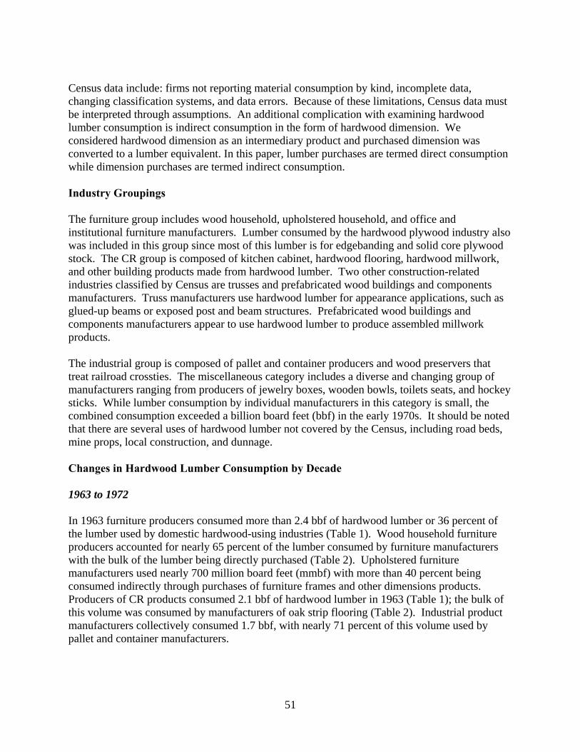
51

Census data include: firms not reporting material consumption by kind, incomplete data, changing classification systems, and data errors. Because of these limitations, Census data must be interpreted through assumptions. An additional complication with examining hardwood lumber consumption is indirect consumption in the form of hardwood dimension. We considered hardwood dimension as an intermediary product and purchased dimension was converted to a lumber equivalent. In this paper, lumber purchases are termed direct consumption while dimension purchases are termed indirect consumption. Industry Groupings The furniture group includes wood household, upholstered household, and office and institutional furniture manufacturers. Lumber consumed by the hardwood plywood industry also was included in this group since most of this lumber is for edgebanding and solid core plywood stock. The CR group is composed of kitchen cabinet, hardwood flooring, hardwood millwork, and other building products made from hardwood lumber. Two other construction-related industries classified by Census are trusses and prefabricated wood buildings and components manufacturers. Truss manufacturers use hardwood lumber for appearance applications, such as glued-up beams or exposed post and beam structures. Prefabricated wood buildings and components manufacturers appear to use hardwood lumber to produce assembled millwork products. The industrial group is composed of pallet and container producers and wood preservers that treat railroad crossties. The miscellaneous category includes a diverse and changing group of manufacturers ranging from producers of jewelry boxes, wooden bowls, toilets seats, and hockey sticks. While lumber consumption by individual manufacturers in this category is small, the combined consumption exceeded a billion board feet (bbf) in the early 1970s. It should be noted that there are several uses of hardwood lumber not covered by the Census, including road beds, mine props, local construction, and dunnage. Changes in Hardwood Lumber Consumption by Decade 1963 to 1972 In 1963 furniture producers consumed more than 2.4 bbf of hardwood lumber or 36 percent of the lumber used by domestic hardwood-using industries (Table 1). Wood household furniture producers accounted for nearly 65 percent of the lumber consumed by furniture manufacturers with the bulk of the lumber being directly purchased (Table 2). Upholstered furniture manufacturers used nearly 700 million board feet (mmbf) with more than 40 percent being consumed indirectly through purchases of furniture frames and other dimensions products. Producers of CR products consumed 2.1 bbf of hardwood lumber in 1963 (Table 1); the bulk of this volume was consumed by manufacturers of oak strip flooring (Table 2). Industrial product manufacturers collectively consumed 1.7 bbf, with nearly 71 percent of this volume used by pallet and container manufacturers.

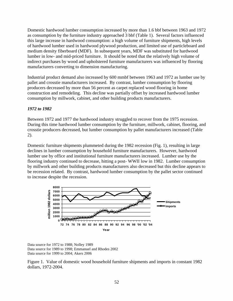
52

Domestic hardwood lumber consumption increased by more than 1.6 bbf between 1963 and 1972 as consumption by the furniture industry approached 3 bbf (Table 1). Several factors influenced this large increase in hardwood consumption: a high volume of furniture shipments, high levels of hardwood lumber used in hardwood plywood production, and limited use of particleboard and medium density fiberboard (MDF). In subsequent years, MDF was substituted for hardwood lumber in low- and mid-priced furniture. It should be noted that the relatively high volume of indirect purchases by wood and upholstered furniture manufacturers was influenced by flooring manufacturers converting to dimension manufacturing. Industrial product demand also increased by 600 mmbf between 1963 and 1972 as lumber use by pallet and crosstie manufacturers increased. By contrast, lumber consumption by flooring producers decreased by more than 56 percent as carpet replaced wood flooring in home construction and remodeling. This decline was partially offset by increased hardwood lumber consumption by millwork, cabinet, and other building products manufacturers. 1972 to 1982 Between 1972 and 1977 the hardwood industry struggled to recover from the 1975 recession. During this time hardwood lumber consumption by the furniture, millwork, cabinet, flooring, and crosstie producers decreased, but lumber consumption by pallet manufacturers increased (Table 2). Domestic furniture shipments plummeted during the 1982 recession (Fig. 1), resulting in large declines in lumber consumption by household furniture manufacturers. However, hardwood lumber use by office and institutional furniture manufacturers increased. Lumber use by the flooring industry continued to decrease, hitting a post- WWII low in 1982. Lumber consumption by millwork and other building products manufacturers also decreased but this decline appears to be recession related. By contrast, hardwood lumber consumption by the pallet sector continued to increase despite the recession.

Data source for 1972 to 1988; Nolley 1989 Data source for 1989 to 1998; Emmanuel and Rhodes 2002 Data source for 1999 to 2004; Akers 2006 Figure 1. Value of domestic wood household furniture shipments and imports in constant 1982 dollars, 1972-2004.

010002000300040005000600070008000

72 74 76 78 80 82 84 86 88 90 92 94 96 98 '00 '02 '04

Year

mill

ion

1982

dol

lars

ShipmentsImports

53

1982 to 1992 Between 1982 and 1987 hardwood lumber consumption by domestic manufacturers increased by 2.4 bbf. More than 40 percent of this increase was the result of increased lumber consumption by CR product manufacturers. Furniture manufacturers also increased hardwood lumber consumption during the 1980s, but these increases were relatively small as furniture imports increased. Lumber consumption decreased slightly between 1987 and 1992, but this decrease was disparate across and within industries. Hardwood lumber use by the wood household furniture manufacturers remained steady as imports increased (Table 1, Fig. 1). By contrast, consumption by upholstered and office furniture manufacturers increased. Similarly, consumption by flooring and kitchen cabinet manufacturers increased. The largest decrease in lumber consumption was by industrial products manufacturers because of reduced pallet and crossties production. 1992 to 2002 In the mid-1990s, domestic hardwood lumber consumption surged as use by CR producers increased. The increase of nearly 1 bbf in lumber use by this industry group between 1992 and 1997 was largely the result of increased use of hardwood material in home construction and larger homes being built. By 1997, CR usage had surpassed that of the furniture group. However, industrial product manufacturers continued to be the largest users of hardwood lumber, consuming nearly 5 bbf in 1997. Hardwood lumber consumption by the furniture industry rebounded in 1997; however, the 13 percent increase in wood household furniture shipments was considerably smaller than the 75 percent increase in imported furniture (Fig. 1). The decreased use of lumber by upholstered furniture manufacturers was the result of increased use of plywood in furniture frames. Between 1997 and 2002, furniture manufacturers’ consumption of hardwood lumber decreased by 600 mmbf as numerous domestic furniture plants closed because they could not compete with offshore producers (Schuler and Buehlmann 2003). Hardwood lumber consumption by the pallet industry also declined 400 mmbf between 1997 and 2002. However, this reduction was not a function of reduced pallet use but increased recycling of pallets and pallet parts. By contrast, hardwood lumber consumption by CR product manufacturers increased by more than 400 mmbf as home construction and remodeling activities increased to 4.1 bbf in 2002. Conclusions Hardwood lumber consumption by domestic manufacturing industries increased by nearly 78 percent between the early 1960s and late 1990s before declining in the current century. Still, there is little consistency in hardwood lumber demand when examining specific manufacturing categories or larger industry groups. Industrial product producers were the only industry group that consistently increased lumber use between 1963 and 1997. This seems consistent with a generally expanding economy during this period. However, while consumption of lumber by the

54

pallet and container industry increased on a continual basis, consumption by the crosstie industry has been more erratic. Although the furniture industry has long been considered the dominant consumer of hardwood lumber, the proportion of hardwood lumber consumed by these manufacturers has steadily declined since the 1970s. Increased imports of wood furniture and the substitution of panel products for lumber caused relative consumption by the furniture industry to drop to 18 percent by 2002. Lumber demand by construction and remodeling product manufacturers declined between 1963 and 1982 due to reduced flooring production. Since 1982, there has been a steady increase in lumber consumption by these manufacturers as purchasers of residential homes continue to demand hardwood flooring, cabinets, and millwork. Hardwood lumber consumption by the CR group surpassed consumption in furniture in the late 1990s. The variability in hardwood lumber demand over the past 4 decades demonstrates the dynamic and unpredictable nature of hardwood markets. Much of this unpredictability could be related to the fact that higher quality hardwood is consumed by industries that produce esthetic or fashion-based products that cycle in and out of popularity. Material and product substitution also has played a major role in shaping some hardwood markets. In 1963, veneered tabletops usually were constructed using hardwood plywood with a lumber core. By the 1980s, particleboard and other composite substrates had replaced lumber. In the 1960s, carpeting became the favorite floor covering but wood floor reemerged as a desirable product in the 1990s. Of all of the impacts on hardwood lumber demand over the past 40 years, none seems more influential than globalization. Sectors less sensitive to imported products, e.g., low-end industrial products and construction-related products that can be customized, have fared far better than the domestic furniture industry, where products have been manufactured as commodities with a large labor component. It is interesting that consumption by industrial product manufacturers has increased the most consistently over time and corresponded well with the expanding U.S. and world economies and the need to transport and store manufactured goods. Literature Cited Akers, M. 2006. Bulletin of hardwood markets statistics: first half 2005. Res. Note NE-386.

Newtown Square, PA:. USDA For. Serv., Northeast. Res. Stn. 24 p. Emanuel, D. and C. Rhodes. 2002. Bulletin of hardwood markets statistics: 1989 - 2000. Res.

Note NE-375:Newtown Square, PA: USDA For., Serv. Northeast. Res. Stn. 24 p. Nolley, J. 1989. Bulletin of hardwood markets statistics: Fall 1988. Gen. Tech. Rep. NE-122.

Broomall, PA: USDA For. Serv., Northeast. For. Exp. Stn. 29p.

55

Schuler, A. and U. Buehlmann. 2003. Identifying future competitive business strategies for the U.S. furniture industry: benchmarking and paradigm shifts. Gen. Tech. Rep. NE-304. Newtown Square, PA: USDA For. Serv., Northeast. Res. Stn.15 p.

USDC Bureau of the Census 1963-1992. Bureau of the Census, Census of Manufactures, for

years 1963 to 1992, U.S. Department of Commerce, Washington, D.C. USDC US Census Bureau 2004. Census of Manufactures 2002, U.S. Department of Commerce,

Washington, D.C.

56

Unintended Consequences: Effect of the American Jobs Creation Act Reforestation Incentives on Family Forest Owners in the South

John L. Greene1 and Thomas J. Straka2

Abstract: The American Jobs Creation Act of 2004 rewrote the reforestation tax incentives available to private forest owners. Owners can now deduct outright reforestation costs up to $10,000 per year for each qualified timber property and amortize any additional amount over 8 tax years. To assess the economic effect of the new incentives on forest owners, the authors developed spreadsheets to calculate after-tax Bare Land Value (BLV) for representative management plans for family forests in the South under three tax situations: no reforestation incentives, the incentives under the previous law, and the incentives under the current law. We found that compared to no tax incentive, the current law chiefly benefits owners with high non-timber income, increasing BLV by roughly 20 percent, compared to 5–10 percent for owners with low or median income. Compared to the previous law, the current law chiefly benefits owners with large forest holdings, increasing BLV by roughly 5–15 percent, while decreasing BLV for owners with small holdings. These findings are significant since it appears Congress intended that the new incentives continue to benefit primarily “small woodland owners” with modest incomes and forest holdings. Keywords: Reforestation, tax, deduction, incentive, financial analysis Introduction

The American Jobs Creation Act of 2004 (P.L. 108-357) rewrote the reforestation tax incentives available to private forestland owners. Under the previous law (P.L. 96-451) owners could take a 10-percent tax credit on and amortize (write off) qualifying reforestation costs up to $10,000 per year over 8 tax years.1 Under the new law, owners can deduct outright qualifying reforestation costs up to $10,000 per year for each qualified timber property and amortize any additional amount, again over 8 tax years. The reforestation tax credit is eliminated.

With its $10,000 cap on both the tax credit and amortization provisions, the previous law was designed to benefit primarily “small woodland owners.” In contrast, the new law benefits owners of forest holdings of all sizes, large and small, although it appears Congress intended that it continue to benefit “small woodland owners” with modest incomes and forest holdings (RIA 2004).

1 Research Forester, USDA Forest Service, Southern Research Station, 701 Loyola Ave., Room T-10034, New Orleans, LA 70113-1931, jgreene01@fs.fed.us, (504) 589-7130 (v). 2 Professor, Clemson University, Department of Forestry and Natural Resources, P.O. Box 340317, Clemson, SC 29634-0317, tstraka@clemson.edu, (864) 656-4827 (v).

57

Procedure

To demonstrate the effect of the new reforestation tax incentive we developed spreadsheets to calculate after-tax Bare Land Value (BLV) for a representative southern pine management plan under three tax situations and five combinations of forest size and non-timber income.

The tax situations used were:

• No reforestation incentives; • The incentives under the previous law (P.L. 96-451); and • The incentives under the current law (P.L. 108-357).

The combinations of forest size and owner income used were:

• Low income owners with a small forest holding; • Median income owners with a small forest holding; • Median income owners with a large forest holding; • High income owners with a small forest holding; and • High income owners with a large forest holding.

The spreadsheets calculated on a year-by-year basis the net financial effect of owning and managing a forest holding under each tax situation and each combination of forest size and owner income. Included were the costs of site preparation and planting; property tax; the effect on federal and state income taxes of deducting forest management expenses and using any reforestation incentives; and the returns, costs, harvest taxes, and federal and state capital gain taxes resulting from timber harvests. The annual net cost and return figures were discounted to the beginning of the rotation using the owners’ personal discount rate (see below), and summed to calculate after-tax per-acre BLV.

Non-timber income was assumed to be $20,000 annually for the low income scenarios, $60,000 for the median income scenarios, and $180,000 for the high income scenarios. The median figure closely approximates average 2005 disposable personal income for a two-person household (Council of Economic Advisors 2006). Holding size was assumed to be 40 acres for the small holding scenarios and 400 acres for the large holding scenarios.

The forest management plan used is shown in Table 1. The plan itself was taken from USDA Forest Service Research Paper SO-255 (Busby and others 1990). Management costs were adapted from the Forest Landowner 34th Manual Edition (DuBois and others 2003), and stumpage prices were 5-year regional averages from the Timber Mart-South Market Newsletter (Timber Mart-South 2001–2005).

The forest holding was assumed to consist of a single, even-age stand constituting one qualified timber property. The forest owners were assumed to be a married couple who file joint federal and state tax returns, qualify as material participants in their forest enterprise, have itemized deductions equal to the standard deduction, and use a personal discount rate of 4 percent, real (with inflation factored out).

The owners also were assumed to be subject to the following federal, state, and local taxes:

• Federal income and capital gains taxes at 2005 rates;

58

• State income and capital gains taxes at 25 percent of the federal rates; • A property tax equal to $5 per acre per year; and • A harvest tax equal to 2.5 percent of the gross stumpage price.

Table 1. Forest management plan, management costs, and stumpage returns used in the analysis. a. Forest Management Plan Year 0: Site preparation and planting Year 15: Commercial thinning.............................. 3.85 cords per acre pulpwood 0.75 cords per acre chip-n-saw 0.00 MBF per acre sawtimber Year 30: Final harvest ........................................... 12.21 cords per acre pulpwood 25.44 cords per acre chip-n-saw 2.89 MBF per acre sawtimber b. Management Costs Site preparation and planting ................................ $ 270.00 per acre Sale administration cost ........................................ 10% of gross stumpage price c. Product Prices Pulpwood stumpage .............................................. $ 18.00 per cord Chip-n-saw stumpage............................................ $ 62.50 per cord Sawtimber stumpage ............................................. $ 277.00 per MBF

This marginal approach enabled us to isolate and analyze the effect of the change in reforestation tax incentives on private forest owners with various sizes of forest holdings and income levels. The remainder of the paper presents and discusses the study findings. Results

No Reforestation Incentives

Among the first findings of the study was that after-tax BLV varies with owner income and forest size – compare for example, the after-tax BLV values in Table 2, Tax Situation 1. The variation results from the progressive structure of federal and state taxes and from the effect of forest management deductions on forest owners’ taxable non-timber income.

In the no reforestation incentive tax situation, reforestation costs are carried as basis until they can be deducted against timber harvest income. BLV is highest in the low income, small holding ownership scenario, for reasons related to owners’ low non-timber income. First, deductions for property and harvest taxes removed a larger fraction of the owners’ non-timber income from taxable income. Second, because capital gains are allocated between the 5- and 15-percent federal tax rates based on total income, most of these owners’ timber capital gains were taxed at the lower rate (Table 2, Tax Situation 1).

In the median income ownership scenarios, deductions for property and harvest taxes removed a smaller fraction of the owners’ non-timber income from taxable income, resulting in lower

59

BLVs. Comparing the two, about one-fourth of the median income, small holding owners’ timber capital gains were taxed at the lower, 5-percent federal rate, resulting in a higher BLV. About nine-tenths of the median income, large holding owners’ timber capital gains were taxed at the higher, 15-percent federal rate, resulting in a lower BLV (Table 2, Tax Situation 1).

In the high income ownership scenarios, deductions for property and harvest taxes removed a still smaller fraction of the owners’ non-timber income from taxable income. All of these owners’ timber capital gains were taxed at the 15-percent federal rate, resulting in identical BLVs (Table 2, Tax Situation 1). Previous Law

In the previous law tax situation, the need to carry reforestation costs as basis is reduced or eliminated by the reforestation tax credit and amortization provisions. After-tax BLVs increased over the no-incentive tax situation in all five ownership scenarios, with the greatest increases occurring in the three small-holding ownership scenarios. In these scenarios, the law’s reforestation tax credit provision – a dollar-for-dollar reduction in tax due – effectively shielded a portion of the owners’ non-timber income from federal and state income taxes. More important from an economic standpoint, the amortization provision enabled the owners to recover nearly all of their reforestation costs during the first 8 years of a rotation (Table 2, Tax Situation 2).

Among the small-holding ownership scenarios, the low income owners saw the lowest increase in BLV, for two reasons. First, they had to spread their reforestation tax credit over 6 tax years because it exceeded their income tax due, and second their amortization deductions were taken against non-timber income in a low federal tax bracket (10 percent). The high income owners saw the highest increase in BLV because their amortization deductions were taken against non-timber income in a high federal tax bracket (28 percent; Table 2, Tax Situation 2).

Much smaller increases in BLV occurred in the two large-holding scenarios. The $10,000 cap on both the reforestation tax credit and amortization provisions allowed the owners to recover only about one-tenth of their reforestation costs in the early years of a rotation; the rest of the costs had to be carried as basis until timber was harvested. Comparing the scenarios, the high income, large holding owners took the amortization deduction against non-timber income in a high federal tax bracket (28 percent), resulting in a larger increase in BLV (Table 2, Tax Situation 2). Current Law

With its reforestation deduction and unlimited amortization provisions the current law eliminates the need to carry any reforestation costs beyond the first 8 years of a rotation. As under the previous law, BLVs increased over the no-incentive tax situation in all five ownership scenarios. The pattern of the increases, however, was quite different. The greatest increases occurred in ownership scenarios characterized by high non-timber income, because these owners took the reforestation and amortization deductions against non-timber income in a high federal tax bracket (28 percent; Table 2, Tax Situation 3).

60

Table 2. Comparison of the financial effect of reforestation tax incentives on owners under differing assumptions about forest size and non-timber income (all after-tax BLVs are on a per-acre basis).

Tax Situation

1: No Reforestation Incentives 2: Previous Law (P.L. 96-451) 3: Current Law (P.L. 108-357) Increase Over Increase Over Increase Over

Ownership Scenario After-Tax

BLV Tax Situation

1 After-Tax

BLV Tax Situation

1 After-Tax

BLV Tax Situation

1 Low income, small holding ....... 504.48 -- 566.81 12.4% 526.54 4.4% Median income, small holding .. 458.54 -- 538.07 17.3% 507.74 10.7% Median income, large holding... 438.73 -- 446.55 1.8% 474.84 8.2% High income, small holding ...... 453.69 -- 574.73 26.7% 557.17 22.8% High income, large holding ....... 453.69 -- 465.79 2.7% 543.44 19.8%

In the high income, small holding scenario the owners benefited most from the law’s reforestation deduction provision, which enabled them to recover nearly all of their reforestation costs in the year they occurred – little was left to amortize. In the high income, large holding scenario the owners benefited most from the law’s unlimited amortization provision, which allowed them to recover reforestation costs above the $10,000 deduction amount during the first 8 years of a rotation (Table 2; Tax Situation 3).

After-tax BLV increased by roughly half as much in the scenarios characterized by median non-timber income, because in these scenarios the reforestation and amortization deductions were taken against non-timber income in a lower federal tax bracket (15 pct). The median income, small holding scenario mirrored the small holding scenario above, with the owners benefiting most from the law’s reforestation deduction provision. The median income, large holding scenario mirrored the large holding scenario above, with the owners benefiting most from the law’s unlimited amortization provision (15 pct; Table 2, Tax Situation 3).

The increase in BLV was lowest for the low income, small holding scenario, again for two reasons. First, the owners were not able to make full use of the $10,000 reforestation deduction because it exceeded their taxable income by a sizeable amount; like large holding owners, they recovered most of their reforestation expenses through amortization. Second, both the reforestation and amortization deductions were taken against non-timber income in a low federal tax bracket (10 pct; Table 2, Tax Situation 3).

61

Note that after-tax BLVs for the three small-holding scenarios are lower under current law than under the previous law. This indicates that regardless of income level, for owners of small forest holdings the current law’s more generous provisions for reforestation and amortization deductions are outweighed by the loss of the previous law’s reforestation tax credit. Discussion

After-tax BLV varies with size of the forest holding and amount of the forest owners’ non-timber income. The variation results from the progressive structure of federal and state taxes – which increase with income for both ordinary income and capital gains – and from the effect of forest management deductions on owners’ taxable non-timber income.

Compared to no reforestation incentives, both the previous law and current law produce higher after-tax BLVs in all five ownership scenarios. The pattern of the increases, however, is quite different. The previous law primarily benefited owners with small forest holdings. The law’s reforestation tax credit effectively shielded a portion of these owners’ non-timber income from federal and state income taxes, and its amortization provision enabled them to recover nearly all their reforestation costs during the early years of a rotation.

Compared to no reforestation incentives, the current law primarily benefits owners with high non-timber income, because the tax savings from the $10,000 reforestation deduction and unlimited amortization provisions are greatest for owners in high tax brackets. Compared to the earlier reforestation incentives, the current law primarily benefits owners with large forest holdings, because elimination of the $10,000 cap on the provisions lets them recover all of their reforestation costs in the early years of a rotation

For owners with small forest holdings, after-tax BLVs are lower under current law than under the previous law. For these owners, the current law’s more generous reforestation and amortization deduction provisions are outweighed by the loss of the reforestation tax credit. These findings are significant since it appears Congress intended that the new incentives continue to benefit primarily “small woodland owners” with modest incomes and forest holdings. Endnote 1 The regulations for the amortization provision required than forest owners reduce the amount

amortized by half of any reforestation tax credit they took. Literature Cited

Busby, R.L., K.B. Ward, and V.C. Baldwin, Jr. 1990. COMPUTE_MERCHLOB: A Growth and Yield Prediction System with a Merchandizing Optimizer for Planted Loblolly Pine in the West Gulf Region. Research Paper SO-255. USDA Forest Service, Southern Forest Experiment Station, New Orleans, Louisiana. 22 pages.

Council of Economic Advisors. 2006. Economic Indicators: March 2006. Prepared for the Joint Economic Committee, 109th Congress, 2nd Session. U.S. Government Printing Office, Washington, D.C. 38 pages

62

DuBois, M.R., T.J. Straka, S.D. Crim, and L.J. Robinson. 2003. Costs and cost trends for forestry practices in the South. Forest Landowner 34th Manual Edition. 62(2): 3–9.

RIA (Research Institute of America). 2004. RIA’s Complete Analysis of the American Jobs Creation Act of 2004: With Code Sections as Amended and Committee Reports. Research Institute of America, New York. 3,525 pages.

Timber Mart-South. 2000–2005. Timber Mart-South Market Newsletter. Daniel B. Warnell School of Forest Resources, The University of Georgia, Athens, Georgia.

63

Impacts of Timberland Ownership on Stumpage Market in the US South

Xianchun Liao1 and Yaoqi Zhang2

Abstract: This paper focuses on the short run price elasticities for stumpage market by comparing forest industry (FI) and nonindustrial private forest (NIPF). An econometric model is derived under the framework of profit maximization. A two-stage least squares (2SLS) technique with time series data from 1953 to 2002 is employed in this study. The estimated results show that supply price elasticities of 0.70 for sawtimber and 0.90 for pulpwood for FI owners are larger than those of 0.29 for sawtimber and 0.32 for pulpwood for NIPF owners, which, in general, are within the price elasticity range from previous studies. Keywords: Profit maximization model, two-stage least squares, price elasticity, forest industry, non-industrial private forest Introduction Almost 25% of timber removal in the world came from the US (FAO 2005) and more than 62% of softwood roundwood products in the US were from the South in 2002 (Smith et al. 2004). In the US South, a large share of the regional softwood production (34%) came from the small share of forested area (17%) owned by forest industry (FI), while a share of the production (62%) came from a much large share of forestlands (71%) held by nonindustrial private forest (NIPF) in 2002 (Smith et al. 2004). Understanding the difference in production behavior between FI and NIPF has been a concern in the forestry literature and an important aspect in public policy and management plan. For example, price elasticities of stumpage play significant roles in measuring market and economic impacts of Sustainable Forestry Initiative by American Forest and Paper Association on stumpage market in the U.S. South in 1994 (Brown and Zhang 2005). Modeling the stumpage market is also useful for assessing the effects of public intervention attempting to improve NIPF output (e.g. Boyd and Hyde 1989, Hardie and Parks 1996). While many studies estimated short-run supply price elasticities for stumpage market (e.g., Brännlund et al. 1985, Newman 1987, Carter 1992, Polyakov et al. 2005), few studies conduct research on supply elasticities for industry and NIPF timberlands separately (e.g. Adams and Haynes 1980, Haynes and Adams 1985, Newman and Wear 1993, and Liao 2007). For example, Adams and Haynes (1980) estimated a combined pulpwood/sawtimber supply elasticity for FI and NIPF. It is clear that different species have different biological characteristics, which influence timber growing stock. In addition, the study has small samples covering only 20-30 annual observations. The small observations with time series data might cause the coefficients of a simultaneous system of equations (SSE) to be sensitive to its specification and even 1 Research Associate, School of Forestry and Wildlife Sciences, Auburn University, AL 36849, liaoxia@auburn.edu, (334) 844 8042 (v), (334) 844-1084 (fax). 2 Assistant Professor, School of Forestry and Wildlife Sciences, Auburn University, AL 36849, Yaoqi.Zhang@auburn.edu, (334) 844-1041 (v), (334) 844-1084 (fax).

64

inconsistent (Wooldridge 2000). Although Newman and Wear (1993) gave the most recent supply elasticities for FI and NIPF, the study used cross-sectional data, which might not pick up all the past dynamical variability between stumpage supply and price. Moreover, the study treated stumpage prices as exogenous variables, which might not have economic justification because prices would be endogenous in the forest sector in general. This study estimates stumpage supply in the US South by comparing the production behavior between FI and NIPF. This study hypothesizes that NIPF owners’ behavior is the same as industrial owners who pursue profit maximization. A two stage least squares (2SLS) method with time series data from 1953 to 2002 is applied to estimate the model. The paper is organized as follows. First, the theoretical model of stumpage supply is presented. Then, the data sources are presented and the empirical estimation using 2SLS follows. Next, the regression results are interpreted. The study ends with summary and conclusion. Data Sources Data sources are described and summarized in Table 1– 2. Softwood stumpage is the total quantity of softwood timber from the US South. Data for softwood harvest on FI and NIPF for 1953-2002 is from Adams et al. (2006), but the data combines pulpwood/sawtimber. Pine pulpwood production for 13 southern states is from the Southeastern and Southern Forest Experiment Stations of the USDA Forest Service for 1950-2002, but the data is not classified by two ownerships (FI and NIPF). A ratio of sawtimber to pulpwood for 1950-1980 is from Adams et al. (1988) and for 1981-2002 estimated according to the source from the Southeastern and Southern Forest Experiment Stations. Then production is allocated for sawtimber and pulpwood by the two ownerships, respectively. The average volume-weighted stumpage price of softwood timber for 1950-1976 is from Ulrich (1989) and for 1977-2002 from Howard (2003). Net volume of softwood sawtimber for 1950-2002 is from Smith et al. (1997, p168) and total volume is from Smith et al. (2002, p73) by two ownerships (FI and NIPF). Because the USDA Forest Service reports inventory data at approximate ten years interval. The missing data is found based on the formula from Newman (1987). The formula is specified as the following:

)([ **1 SSGvv ttt −−+= − where G* is the average annual net growth between survey years and

S* is the average stumpage production between survey years. The producer price index of the paper and allied products is viewed as an instrument for pulpwood price equation and lumber price index for sawtimber price system from the Bureau of Labor and Statistics (BLS). All data are annual and the time series cover the period from 1953 to 2002 (50 observations). The deflator is the Producer Price Index used for all prices from the US Bureau of Labor Statistics (BLS) (1982=100). Theoretical Framework The stumpage market is assumed to close to competitive because the market concentration is unlikely in the US South. An aggregate stumpage supply is derived from a profit maximization model, following the early authors’ framework of Johansson and Löfgren (1985), and Brännlund et al. (1985). The present profit function can be defined as:

65

)(),,(,

io

io

io

io

io

LQ

io

io

io

io vLwQpMaxvwp

ii−=π (1)

where i = 1 for sawtimber and 2 for pulpwood, o = 1 for FI and 2 for NIPF, Q is the set of feasible cutting possibilities, p is the stumpage price, w is per unit harvesting labor cost, L is labor input, v is the inventory. Timber production is constrained by inventory. Assuming that the present profit function is convex in p and w and applying Hotelling’s lemma, the firm’s supply of the stumpage in period t is a function of market price and the prices of all inputs in production. The supply function is found by taking the first derivative of the profit function. Thus,

),,( io

io

io

ioi

o

io vwpQ

p=

∂∂π (2)

),,( io

io

io

ioi

o

io vwpL

w−=

∂∂π (3)

Because the data about harvesting cost is not available, the amount of growing stock serves as an inverse proxy for it, as suggested by Newman (1987). The reasoning behind is that growing stock is viewed as a measure of accumulated forestry capital adjusted through time by forest regeneration costs, forest growth, and timber cutting (Newman and Wear 1993). Thus, the supply specification is as the following:

),(Qiojt

++

= iojt

iojt

iojt vpQ (4)

The own price for the pulpwood has a positive effect on supply. Timber inventory has a positive effect on the output because the marginal harvesting costs decrease as inventory increases. If all the forest owners in the region maintain the same production, the regional stumpage supply specification can be found by aggregating the N individual forest owner’s production functions. Thus,

),(),(1

iojt

iojt

N

j

iojt

iot

iot

iot vpQvpQ ∑

=

= (5)

The equation serves as a theoretic model for this analysis and shows that the stumpage supply depends on own price and inventory. Keep in mind, transportation costs are assumed a relatively constant fraction of the stumpage price and do not affect the short-run supply in the region as well. Empirical Model In the empirical analysis, equation 5 is adapted in the following way. A two-stage least squares (2SLS) procedure is used to correct for endogenous bias in the stumpage supply model, because market price and output quantity may be determined jointly. The 2SLS approach includes a first stage regression, estimating how market price changes are influenced by economic variables.

66

Then predicted price values from this first stage regression are used in place of output price in the second stage. The two-stage empirical model is as follows: Stage 1

iot

iot

iot

io

io Zv εϕβα +++= 1

iotp (6)

Stage 2

iot

iot

iot

io

io pv εϕβα +++=

∧

1iotQ (7)

where iotZ is an instrumental variable for stumpage price.

∧iotp is predicted values for market price

at year t from first stage regression. Instrument choices show reasonable in this study. An instrument should be (a) correlated with the endogenous explanatory variable and (b) uncorrelated with the error term in the equation. We regress pulpwood stumpage price on paper and allied products price index (instrument variable) and other independent variables using a reduced-form. The results show that the instrument variable (IV) is correlated (coefficient =0.09) with pulpwood price at the 5% significant level (p-value=0.011) and R2 is 0.73. Unfortunately, we cannot test (b) using the data because it is impossible to check the correlation between IV and the error term, which is not observable, but appealing by economic assumption (Wooldridge 2000, p 463). Based on economic theory, final paper price does not have effect on pulpwood supply, which implicitly assume that there is no correlation between the IV and the error term. Likewise, we regress sawtimber stumpage price on lumber price (instrument variable) and other independent variables using a reduced-form. The results show that the instrument variable is correlated (coefficient =0.64) with pulpwood price at the 1% significant level (p-value=0.0001) and R2 is 0.82. Empirical Results Linear and log-linear forms have been estimated by two stage least squares (2SLS). The linear form results are presented here because it outperforms better than log-linear form in terms of coefficient significant. Table 3 presents coefficients of the estimated profit maximization function for FI and NIPF. Overall, the R2 values for all equations are high, which means the explanatory variables significantly explain the dependent variables. The coefficients have the expected sign and all of them are significant at the 5% or 10% levels for both FI and NIPF ownerships. Our results show that all own prices are significantly positive at the 5% level, which is consistent with the literature in that an increased own price of sawtimber or pulpwood increases the supply of the assortment (e.g. Brännlund et al. 1985). Timber inventory variables are significantly positive at the 5% or 10% level, which is also consistent with the claims in the literature that the marginal harvesting costs decrease as inventory increases (e.g., Newman 1987). The positive cross-price effects between sawtimber and pulpwood for FI and between pulpwood and sawtimber for NIPF indicate that they are gross complement in the short run. However, the

67

effects between pulpwood and sawtimber for FI and between sawtimber and pulpwood for NIPF are insignificant and excluded from the equations, which demonstrate that there is neither gross substitute nor complement in the short run. A possible explanation is that cross price has both substitute and joint production effects. The substitute effect will lead a shift from pulpwood to sawtimber, while joint effect indicates that an increase in final cuttings will increase both sawtimber and pulpwood supply (Brännlund et al. 1985, Newman 1987). Which effect is larger depends on empirical analysis. To measure the impacts of the explanatory variables on stumpage supply, the elasticities are calculated at the mean of the variables (see table 4). The own price elasticities are generally high: 0.70 for sawtimber and 0.90 for pulpwood for FI owners, while they are low: 0.29 for sawtimber and 0.32 for pulpwood for NIPF owners. The respective elasticities are significantly different between the two ownerships; however, the result is consistent with those reported for the US South (Newman and Wear 1993). The possible explanation is that FI owners manage timberland exclusively for timber production, while NIPF owners who do not own wood processing facilities produce both timber and nontimber benefits. Pulpwood supply shows relatively more elastic responses to own price than sawtimber for both ownerships. The possible explanation is that pulpwood can be produced from growing stocks at almost any age whereas sawtimber can only be produced from larger trees at older stage (Newman and Wear 1993). Inventory elasticities for FI are higher than those for NIPF, which is consistent with the literature in that NIPF owners obtain nontimber benefits from the growing stock remaining in place while FI owners perceive financial profits from the timber. The estimated elasticities in this study can only be partially compared with existing values in the literature because of difference in methodology, data sources and regional focus. Table 5 compares price and inventory elasticities from this study and other studies for the US South. For example, Adams and Haynes (1980) estimated a combined sawtimber/pulpwood supply elasticity for the southeast of 0.47 for FI and 0.39 for NIPF and the south-central of 0.47 for FI and 0.30 for NIPF. Only Newman and Wear (1993) estimated supply price elasticities for sawtimber (0.27 for FI and 0.22 for NIPF) and pulpwood (0.58 for FI and 0.33 for NIPF) in the Southeast separately. Few studies on supply price elasticities in the US South exist in the literature in terms of the two ownerships and the two timber categories. Concluding Remarks Using profit maximization model with time series data from 1953 to 2002, this study estimated stumpage supply for both forest industry and NIPF owners in the US South. The results show that supply price elasticities of 0.70 for sawtimber and 0.90 for pulpwood for FI owners are larger than those of 0.29 for sawtimber and 0.32 for pulpwood for NIPF owners, which in general are relatively larger than previous studies (e.g. Adams and Haynes 1980, Newman and Wear 1993). Pulpwood supply shows relatively more elastic responses to own price than sawtimber regardless of ownership. This study makes two contributions to the US timber supply literature. First, a separated stumpage supply function for FI and NIPF is estimated, while most previous studies combined

68

the two ownerships together. Second, a separated stumpage category (sawtimber and pulpwood) is employed while most previous studies did combine the two species together. The finding suggests that profit maximization model is appropriate for NIPF owners at the aggregate level, although they are not able to respond to changing market conditions as strongly as FI owners. In addition, using previous small price elasticities for FI to measure market and economic impacts of Sustainable Forestry Initiative may cause biased welfare implication. Moreover, public efforts to improve NIPF output might not be efficient because NIPF owners have relatively less responses to market signal than FI owners. Further research is needed to examine landowner’s behavior at individual level.

Literature Cited Adams D.M., K.C. Jackson, and R.W. Haynes. 1988. Production, Consumption and Prices of

Softwood Products in North America: Regional Time Series Data, 1950–1985. Resource Bull. PNW-RB-151, USDA For. Serv. Pacific Northwest Res. Stn., Portland, OR. 49 p.

Adams, D.M. and R.W. Haynes. 1980. The 1980 softwood timber market assessment model:

Structure, projections, and policy simulations. For. Sci. Monograph 22:64. 64 p. Adams, D.M., R.W. Haynes, and A.J. Daigneault. 2006. Estimated timber harvest by U.S. region

and ownership, 1950-2002. Resource Bull. PNW-GTR-659, USDA For. Serv. Pacific Northwest Res. Stn., Portland, OR. 64p.

Boyd, R. and W.F. Hyde. 1989. Forestry Sector Intervention. Ames, IA: Iowa State Univ. Press. Brännlund, R., P.O. Johansson, and K.G. Löfgren. 1985. An economic analysis of aggregate

sawtimber and pulpwood supply in Sweden. For. Sci. 31: 595-606. Brown, R. and D. Zhang. 2005. Estimating supply elasticity for disaggregated paper products: a

primal approach. For. Sci. 51(6):570-577 Bureau of Economic Analysis. The Producer Price Index (PPI). http://www.bea.doc.gov. Carter D.R. 1992. Effects of supply and demand determinants on pulpwood stumpage quantity

and price in Texas. For. Sci. 38(3):652-660. EViews. 2004. Eviews User’s Manual. Quantitative Micro Software. Food and Agriculture Organization of the United Nations (FAO). FAOSTAT-Forestry 2006.

http://www.fao.org/waicent/portal/statistics_en.asp Hardie, I.W. and P.J. Parks. 1996. Program enrollment and acreage response to reforestation

cost-sharing programs. Land Econ. 72(2):248 –260.

69

Haynes R.W. and D.M. Adams. 1985. Simulations of the Effects of Alternative Assumptions on Demand-Supply Determinants on the Timber Situation in the United States. USDA Forest Service, Forest Resource and Economics Research, Washington, D.C.

Howard, J.L. 2003. U.S. Timber Production, Trade, Consumption, and Price Statistics 1965-

2002. Gen. Tech. Rep. FPL-RP-615. USDA Forest Service, Madison, WI. P.6. Johansson, P.O. and K.G. Löfgren. 1985. The Economics of Forestry and Natural Resources.

Basil Blackwell, Oxford. 300p. Liao, X. 2007. Essays of Forestry Investments in the US and Stumpage Market in the Southern

US. PhD Dissertation. Auburn University. 98 p. Newman, D.H. 1987. An econometric analysis of the southern softwood stumpage market: 1950-

1980. For. Sci. 33(4):932-945. Newman, D.H. and D.N. Wear. 1993. Production economics of private forestry: a comparison of

industrial and nonindustrial forest owners. Am. J. Agric. Econ. 75:674-684. Polyakov, M., L. Teeter, and J.D. Jackson. 2005. Econometric analysis of Alabama's pulpwood

market. For. Prod. J. 55:4-14. Random Lengths. 1974–2001. Forest Product Market Prices and Statistics Yearbook. Annual

Issue, Random Lengths Publications, Inc., Eugene, OR. Smith, W. B., P. D. Miles, J. S. Vissage, and S. A. Pugh. 2004. Forest Resources of the United

States, 2002. U.S. Department of Agriculture, Forest Service, North Central Research Station, St. Paul, MN. Gen. Tech. Rep. NC-241. p73.

Smith, W. B., J. S. Vissage, D. R. Darr, and R.M. Sheffield. 2001. Forest Resources of the

United States, 1997. U.S. Department of Agriculture, Forest Service, North Central Research Station, St. Paul, MN. http://www.ncrs.fed.us. p168.

Ulrich, A.H. 1989. U.S. Timber Production, Trade, Consumption, and Price Statistics 1950-87. Forest Service, U.S. Department of Agriculture. Wooldridge, J.M. 2000. Introductory Econometrics: A Modern Approach. South-Western

College Publishing, Boston, MA. Zhang, D., and W.A. Flick. 2001. Sticks, carrots, and reforestation investment. Land Econ.

77(3):443– 456.

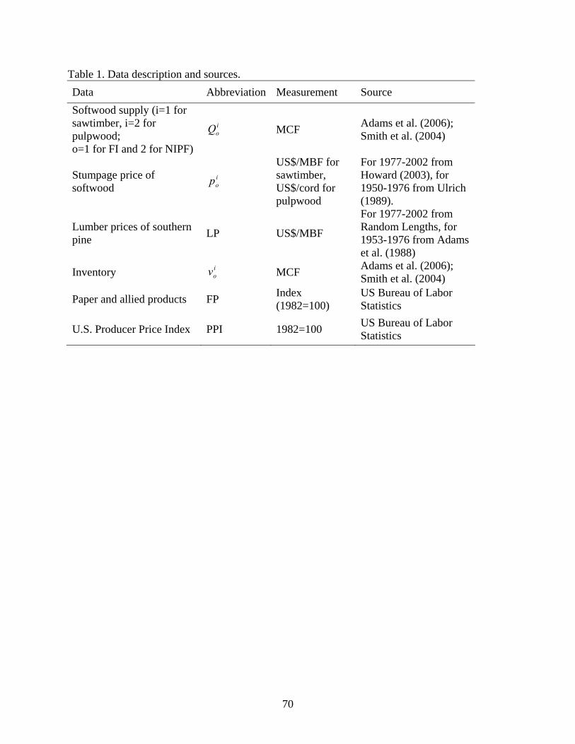
70

Table 1. Data description and sources. Data Abbreviation Measurement Source Softwood supply (i=1 for sawtimber, i=2 for pulpwood; o=1 for FI and 2 for NIPF)

ioQ MCF Adams et al. (2006);

Smith et al. (2004)

Stumpage price of softwood

iop

US$/MBF for sawtimber, US$/cord for pulpwood

For 1977-2002 from Howard (2003), for 1950-1976 from Ulrich (1989).

Lumber prices of southern pine LP US$/MBF

For 1977-2002 from Random Lengths, for 1953-1976 from Adams et al. (1988)

Inventory iov MCF Adams et al. (2006);

Smith et al. (2004)

Paper and allied products FP Index (1982=100)

US Bureau of Labor Statistics

U.S. Producer Price Index PPI 1982=100 US Bureau of Labor Statistics

71

Table 2. Data summary.

Variables Mean Std Min Max

Softwood supply for sawtimber for FI 668.61 308.36 226.38 1096.09

Softwood supply for pulpwood for FI 673.27 225.31 341.52 1047.93

Softwood supply for sawtimber for NIPF 1292.82 383.13 736.15 1975.57

Softwood supply for pulpwood for NIPF 1337.01 199.12 926.86 1723.82

Sawtimber stumpage price

168.49 72.03 85.44 326.98

Pulpwood stumpage price 14.47 3.12 10.62 23.50

Lumber prices of southern pine 241.01 47.61 183.86 353.32

Sawtimber inventory for FI 9901.27 888.47 7973.02 10923.05

Pulpwood inventory for FI 12814.45 1786.28 8567.98 14952.19

Sawtimber inventory for NIPF 24629.09 6113.82 13742.42 31796.53

Pulpwood inventory for NIPF 32938.42 5041.95 22617.58 38324.38

Paper and allied products 79.76 45.87 28.00 159.00

72

Table 3. Estimates of coefficients for both FI and NIPF using profit maximization model. FI NIPF

Variable Sawtimber Pulpwood Sawtimber Pulpwood

Constant -745.02** (334.60)

-853.81**

(118.98)98.33

(108.56)203.23*

(111.07)

Inventory 0.05* (0.029)

0.07**

(0.02)0.03**

(0.01)0.02**

(0.003)

Pulpwood price 28.60** (12.45)

42.03**

(13.01) a 29.70**

(6.72)

Sawtimber price 2.80** (0.66) a 2.23**

(0.87)0.66**

(0.27)Obs. 50 50 50 50

R-squared 0.70 0.74 0.79 0.85

Note: 1. ** and * indicate significances at 5% and 10% levels. 2. Numbers in parentheses denote standard error. 3. All variables are in level form. 4. a means the variable is not significant and dropped off from the model.

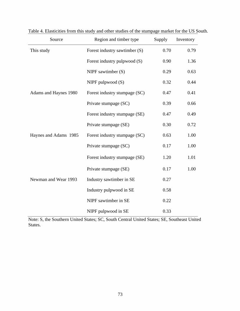
73

Table 4. Elasticities from this study and other studies of the stumpage market for the US South.

Source Region and timber type Supply Inventory

This study Forest industry sawtimber (S) 0.70 0.79

Forest industry pulpwood (S) 0.90 1.36

NIPF sawtimber (S) 0.29 0.63

NIPF pulpwood (S) 0.32 0.44

Adams and Haynes 1980 Forest industry stumpage (SC) 0.47 0.41

Private stumpage (SC) 0.39 0.66

Forest industry stumpage (SE) 0.47 0.49

Private stumpage (SE) 0.30 0.72

Haynes and Adams 1985 Forest industry stumpage (SC) 0.63 1.00

Private stumpage (SC) 0.17 1.00

Forest industry stumpage (SE) 1.20 1.01

Private stumpage (SE) 0.17 1.00

Newman and Wear 1993 Industry sawtimber in SE 0.27

Industry pulpwood in SE 0.58

NIPF sawtimber in SE 0.22

NIPF pulpwood in SE 0.33

Note: S, the Southern United States; SC, South Central United States; SE, Southeast United States.

74

Forest Management Decisions of Nonindustrial Private Forest Landowners of West Virginia

Sudiksha Joshi1 and Kathryn G. Arano2

Abstract: Private forest landowners own the largest share of the forest land in the United States. Majority of the fluctuations in future timber supply have been predicted to result from the activities of these private forest landowners. Examining the forest management decisions of these individuals is therefore important. This paper uses logistic regression models to examine the influence of various landowner and ownership characteristics to the type of forest management activity landowners undertake in their forest. The paper is based on the data from a mail survey conducted in August 2005 to 2100 nonindustrial private forest landowners in West Virginia. Results show that distance of the forest from the place of residence, age, educational level, and household income are influential in determining whether landowners will conduct any form of forest management activity. Also, year of forest land acquisition, presence of written forest management plan, perception of risk in timber investment, prior involvement in the carrying out timber harvesting were found to influence whether or not a landowner would conduct timber harvesting activities. Keywords: NIPF landowners, forest management activities, logistic regression

1 Graduate Research Assistant, Division of Forestry and Natural Resources, West Virginia University, P.O. Box 6125, Morgantown, WV 26506. 2 Assistant Professor, Division of Forestry and Natural Resources, West Virginia University, P. O. Box 6125, Morgantown, WV 26506, Kathryn.Arano@mail.wvu.edu, 304) 293-2941 (v).

75

Nonindustrial Private Forest Landowners’ Participation in Mississippi Forest Resource Development Program*

Xing Sun1, Changyou Sun2, Ian A. Munn3, and Anwar Hussain4

Abastract: Non-industrial private forest (NIPF) landowners are key players in increasing forest productivity and improving forest health. In order for landowners to benefit from government programs intended to improve forest productivity and health, NIPF landowners must first be aware of these programs. This study investigates: 1) what factors are associated with awareness of Mississippi Forest Resource Development Program (FRDP), and 2) given awareness of this program, what factors are associated with participation in FRDP. Examined factors included an array of land, ownership, management, and demographic characteristics. Data were obtained through a phone survey of 2,229 randomly selected NIPF landowners in Mississippi. A two-step discrete/discrete econometric model was used to analyze participation behavior conditional on NIPF landowner knowledge of FRDP. Interest in timber production, education, and membership in forestry organizations influenced NIPF landowner knowledge of incentive programs and were significant predictors of participation. Keywords: Mississippi Forest Resource Development program, nonindustrial private forest landowners, participation behavior, two-step estimation Introduction Non-industrial private forest (NIPF) landowners have been major players in forestry. Nationwide, timberlands are owned by the public (29%), forest industry (13%), and NIPF landowners (58%); they accounted for 11%, 30%, and 59% of the timber harvested in 1996, respectively (Smith et al. 2004). Forests generate timber as raw material for the forest industry, and contribute environmental protection, including soil conservation, carbon storage, and maintenance of air and water quality (Wear and Greis 2002; Alig 2003). Therefore, public agencies have provided NIPF landowners a variety of public assistance programs to help achieve their management goals and meet societal needs. Forestland management can be capital-intensive, particularly when establishing stand. Forests also require a long period of growth before producing income. Public assistance programs can influence the management of NIPF lands, compensate NIPF landowners for high costs of tree

* This manuscript is publication #FO354 of the Forest and Wildlife Research Center, Mississippi State University. 1 Graduate Research Assistant, Department of Forestry, Mississippi State University, Box 9681, Mississippi State,

MS 39762, xs31@msstate.edu, (662) 325-5812 (v), (662) 325-8726 (fax). 2 Assistant Professor, Department of Forestry, Mississippi State University, Box 9681, Mississippi State, MS 39762,

csun@cfr.msstate.edu, (662) 325-7271 (v), (662) 325-8726 (fax). 3 Professor, Department of Forestry, Mississippi State University, Box 9681, Mississippi State, MS 39762,

imunn@cfr.msstate.edu, (662) 325-4546 (v), (662) 325-8726 (fax). 4 Assistant Research Professor, Department of Forestry, Mississippi State University, Box 9681, Mississippi State,

MS 39762, ahussain@cfr.msstat.edu, (662) 325-4259 (v), (662) 325-8726 (fax).

76

planting, and encourage better forest stewardship (Wear and Greis 2002). The goal of many regeneration assistance programs is to reduce the financial burden and encourage NIPF landowners to replant their lands after harvest. Mississippi’s Forest Resource Development Program (FRDP) was established in 1974. It is a state cost-share program for reforestation and timber stand improvement (Nagubadi et al. 1996). The FRDP was developed to provide financial assistance to eligible landowners. This program offsets a landowner’s expenses by sharing the cost of implementing specific forestry practices to produce timber and enhance wildlife development. The FRPD requires that applicants submit a management prescription for the desired treatment area, comply with Mississippi Forestry Commission standards during operations, and maintain practices for at least 10 years. Cost-share payments of FRDP cover 50% to 75% of the total cost of implementing forest practices, with a maximum annual assistance of $5,000 (Gunter et al. 2001). Many studies have been conducted to analyze the behavior of NIPF landowners with regard to their participation in governmental incentive programs and their decisions in silvicultural activities (Amacher et al. 2003). Previous studies generally agreed that these programs have successfully influenced the management of NIPF lands and stimulated more planting activities (Boyd 1984; Nagubadi et al. 1996; Mehmood and Zhang 2001). However, in spite of the benefits, these studies also revealed that NIPF landowners have not always taken advantage of these programs. For example, in a recent study the majority (54.3%) of 427 Mississippi NIPF landowners who regenerated their timber stands following a harvest during the 5-year period from 1994 to 1998 did not receive public cost-sharing funds for regeneration under Forestry Incentive Program (FIP), Mississippi’s FRDP, Conservation Reserve Program (CRP), or Mississippi Reforestation Tax Credit (RTC) (Gunter et al. 2001). Among the 829 landowners that responded to the survey, only 38% were aware of FIP, 24% were aware of FRDP, and 27% were aware of RTC. Many empirical studies have examined NIPF landowner participation behavior in governmental incentive programs. Most commonly these studies have relied on a binary choice model (e.g., (Bell et al. 1994; Nagubadi et al. 1996). Independent variables included owner demographics (e.g., income, education) and land features (e.g., acreage). Landowner participation in public assistance programs has been positively associated with total acres owned, membership in forestry organizations, interest in timber production, income, and location of residence on the landowner’s woodland (Straka et al. 1984; Konyar and Osborn 1990; Nagubadi et al. 1996). Unfortunately, an oversimplified binary model might be inadequate in analyzing landowner participation of incentive programs. As revealed in studies like Gunter et al. (2001), many NIPF landowners were unaware of the existence of these incentive programs. Thus, it is inappropriate to examine landowner participation in government programs that they are not aware of. A binary choice model is derived from an individual’s utility maximization from comparing two choices: participation or no participation. If an individual does not know of the program and did not make the comparison, the dependent variable is actually a missing value, instead of zero. In other words, zero-values for the dependent variable in previous studies might come from two sources: individuals who knew of the program and decided not to participate in it, and individuals who did not know of the program and did not consider the participation at all.

77

The problem with previous studies has originated from their over simplified assumption in the binary choice model with regard to landowners’ behavior. A more suitable approach would be a two-step decision model for a NIPF landowner examining their participation in governmental incentive programs. The innovation is to recognize the reality in forestry that many NIPF landowners are not aware of these programs. The appropriate econometric technique is the sample selection estimation (Greene 2003), which has been widely applied in the literature to other issues (e.g., Lee et al. 2003; Katchova and Miranda 2004). This paper focused on the government program participation behavior of NIPF landowners in Mississippi, a typical southern state where forest industries are important. In Mississippi, NIPF landowners owned 72% of forestlands in the state and produced 67% of state timber outputs in 2002 (Smith et al. 2004). The objective of this study was to examine NIPF landowners’ knowledge of FRDP in Mississippi and their participation in this program from 1996 to 2006. A two-step sample selection model was developed to determine factors associated with landowners’ awareness of FRDP, and conditional on landowners’ awareness, factors affecting the probability of their participation in this program. Conceptual Framework, Survey Data, and Variables Analytical Framework This research used a cross-sectional survey data from Mississippi to determine how land features, forest management experiences, and landowner characteristics influence NIPF landowner knowledge and enrollment probability for FRDP. The study period covered 1996 to 2006. The empirical design was a two-step sample selection model. It assumed that a landowner’s participation in an incentive program was contingent upon whether the landowner was aware of the program.

In the first stage, a landowner’s knowledge of a program, zi, was modeled as a function of variables, wi, that were related to land features, forest management experiences, and landowner characteristics:

(1) Selection equation: ( )i iz g w= where zi was a binary dummy variable that measured the knowledge of landowner i about FRDP. zi was zero if a landowner had no knowledge of the program, and one if the landowner was aware of the program. In the second stage, the landowner decision to participate in FDRP was modeled as a function of land features, forest management experiences, and landowner characteristics, xi:

(2) Outcome equation: yi = f(xi), yi observed only when zi = 1 where yi was a binary variable for landowner participation in FRDP during the study period. yi was zero if a landowner did not participate in program, and one if the landowner participated in the program. The motivation for modeling knowledge (zi) and participation (yi) of NIPF landowners together was that they were related but distinct characteristics, and might be influenced by a same set of factors to a different degree. Therefore, xi might be different from wi.

78

The nature of dependant variables, zi and yi, allowed a bivariate probit model with sample selection. In estimating the model, a predicted value was computed in estimating the selection equation. It was then used in the outcome equation to analyze participating probability. The econometric details of the model are presented in the next section.

Questionnaire and Variables The survey questionnaire was designed to collect information on the variables needed for the empirical analysis as described in Table 1. There were two binary dependent variables, zi and yi. One defined landowner’s knowledge of FRDP; another recorded a landowner’s participation in this program during the study period. The independent variables contained in wi and xi were divided into three groups: land features, forest management experiences, and landowner characteristics. First, three variables were used to represent land features: Acreage, Land type, and Forest type. Acreage was the total land area owned by the landowner in Mississippi. Land type was a binary variable equal to one if the predominant land use was forest, and zero for agricultural or other uses. Forest type was a binary variable equal to one if the predominant forest type was planted pine, and zero for all other types. Second, three variables were constructed to represent forest management experience of the landowner: Year, Timber, and Regeneration. Year was the number of years that the landowner owned the land. Timber was a binary variable representing landowner interest in timber production that equaled one if the landowner was interested in timber production, and zero if not. Regeneration was the number of times that the landowner regenerated during the study period. Finally, eight variables were used to represent demographic characteristics of individual landowner: Age, Education, Income, Employment, Race, Gender, Membership, and Residence. Age represented landowner’s age in 2006. Education was equal to one for those landowners who had bachelor’s or higher degree, and zero otherwise. Income represented the landowner’s household income before taxes in 2005. Employment was equal to one if the landowner was retired, and zero if employed. Race was equal to one for Caucasian landowners, and zero otherwise. Gender was equal to one for male landowners, and zero for females. Membership was equal to one if the landowner was a member of any forestry organization (e.g., Mississippi Forestry Association, Mississippi County Forestry Association, Society of American Foresters, Southern Forestry Association), and zero if not. Residence was equal to one if the landowner resided on their forestland, and zero if not. Methodology The underlying idea of sample selection models is that an outcome variable is only observed if some criterion, defined with respect to a selection variable, is met (Greene 2003). For the research issue in this study, a two-step model with sample selection examines landowner participation in FRDP, conditional on their knowledge of the program. Specifically, in the selection stage, landowner awareness of FRDP (zi) can be estimated with a probit model. In the outcome stage, the binary variable reflects whether or not participation in this program is

79

observed, conditional on landowner awareness of FRDP. Thus, participation (yi) can be modeled using a probit regression, based on landowner knowledge of FRDP. Formally, the two-step model can be expressed as (Greene 2003): (3) Selection equation: z w ei i i

* = +γ *1 if 0; 0 otherwisei iz z= > Pr( ) ( )z wi i= =1 Φ γ Pr( ) ( )z wi i= = −0 1 Φ γ (4) Outcome equation: y xi i i

* = +β ε yi =1 if yi

* >0; 0 otherwise yi observed only when zi =1 where z , y , w and x are variables as defined in the previous section and indexed by landowner i; γ and β are parameters to be estimated; Φ is the normal cumulative distribution function; and e and ε are error terms. In the selection equation, z is a realization of an unobserved continuous variable ( z* ) having a normally distributed, independent error, e , with zero mean and constant variance 2

eσ . In the outcome equation, y is a realization of an unobserved continuous variable ( y* ) and is observed for value of z = 1. y has error ε , with zero mean and constant variance σε

2 . Preliminary analysis revealed that majority of Mississippi’s NIPF landowners who harvested timber did not participate in FRDP. Thus, the binary dependent variable measuring participation, y , was skewed. This motivated us to employ the Gompertz model, which has been used for estimating models with skewed binary data (Greene 2002). Formally, the probabilities of a Gompertz model for y conditional on z determined by a probit model can be expressed as follows (Greene 2002): (5) [ ]{ }Pr( ) exp exp ( )y x wi i i i= = − − −1 β ε γΦ

[ ]{ }Pr( ) exp exp ( )y x wi i i i= = − − − −0 1 β ε γΦ If y is simply regressed on x using observations for which z = 1, the estimates of β will be both biased and inconsistent. In estimating the model, a typical way of addressing this problem involves two steps (Murphy and Topel 1985). The essential part of this model is the correction of the estimated asymptotic covariance matrix for the estimator in the outcome equation for the randomness of the estimator carried forward from the selection equation (Greene 2002). Let V1 be the estimator of the asymptotic covariance matrix for the parameter estimates obtained in the selection equation. Let V2 be the uncorrected covariance matrix computed in the outcome equation, using the parameter estimates obtained in the selection equation as if they were known. Both of these estimators are based on the respective log likelihood functions. In addition, define:

(6) ( ) ( )C

f x f xi ii

n=

⎡

⎣⎢

⎤

⎦⎥⎡

⎣⎢

⎤

⎦⎥=∑

∂∂β

∂∂γ

log log'1

80

( ) ( )

Rf x g wi i

i

n=

⎡

⎣⎢

⎤

⎦⎥⎡

⎣⎢

⎤

⎦⎥=∑

∂∂β

∂∂γ

log log'1

where n is the number of observations. With these in hand, the corrected covariance matrix for the estimator of the outcome equation, V2

*, is as follows: (7) [ ]V V V CV C RV C CV R V2 2 2 1 1 1 2

* ' ' '= + − − . Overall, first estimate the probit model through maximum likelihood and denote the estimated parameter as γ̂ . Then, estimate the Gompertz model in which a predicted value from the model in the selection equation appears on the right hand side of the outcome equation and denote the full set of parameters as β̂ . This predicted value can be expressed as follows:

(8) ( )( )

P Vz

zi

i

11

=−

φ *

*Φ

where ( )φ . and ( )Φ . are, respectively, the density and distribution function for the selection equation. P1V is included in the explanatory variables of the outcome equation, x. When the coefficient of estimated P1V is significant, it implies the parameter estimators for the outcome stage would be biased if two-step estimation procedures were not used. Finally, the two sets of explanatory variables, w and x, can be the same or different. If w is equal to x, or w is a subset of x, then it may be possible to identify the parameters of the outcome equation because of the nonlinearity of the model (Breen 1996). To deal with this issue, two models for FRDP were estimated. First, a general model that treated w and x as the same, respectively in selection and outcome equations, was employed. However, the estimation results for many important explanatory variables were not significant. This suggested a collinearity problem among these variables. Thus, through preliminary analysis, some variables were deleted that had some collinearity with other important explanatory variables but did not affect the outcome stage. Therefore, in a restricted model, the variables in the outcome equation, x, was a subset of the variables in the selection equation, w. Empirical Results Survey Results and Descriptive Statistics of Variables Of the 9,925 landowners contacted by phone, 2,126 owned less than 100 acres and another 2,132 did not harvest timber in the past 10 years, so these landowners were excluded from the survey. There were also 1,110 wrong phone numbers. Other reasons for unsuccessful calls included communication problems, refusal to participate, and deceased owners. A total of 2,229 valid and complete observations were recorded and available for the statistical analysis. The completion rate was 50%, i.e., 2,229 / (9,925 - 2,216 - 2,132 - 1,110).

81

Approximately 40% of the 2,229 landowners were aware of FRDP while 60% did not. This is consistent with the findings from a previous survey in Mississippi (Gunter et al. 2001). Furthermore, among the 2,229 landowners surveyed, a total of 63 NIPF landowners participated in FRDP with 2.8%. The average acreage by surveyed landowners was 507 acres. For most landowners (77%), forestland was the predominant land use. For about half of the landowners (51%), pine was the predominant forest type and the rest had either hardwood or mixed forest types. The average length of ownership was 35 years. Most of these landowners (88%) were interested in timber production. The average number of times a landowner regenerated after harvesting during the survey period was 0.3 per landowner. On average, surveyed landowners were 66 years old, 47% had a bachelor’s or higher degree, and their household income in 2005 was $66,127. In addition, 55% of respondents were retired, 97% were Caucasian, and 70% were male. Approximately, 25% were members of a forestry organization. Finally, 48% resided on their forest lands. To address the study objective, the determinants of landowners’ knowledge of these incentive programs are examined first, followed by examining the determinants of landowners’ participation in these programs. Determinants of Landowner Knowledge of FRDP Regression results on NIPF landowner awareness of FRDP are reported in Table 2. Among the land features, the coefficient for Acreage was positive and significant. Thus, landowners with more land were more likely to be aware of FDRP. Land type and Pine forests were not significant. Among the three measures of land management experience, only the coefficient for Timber was positive and significant, suggesting that landowner interest in timber production motivated them to learn more about the program. Regenerate and Year were not significant. Finally, five demographic characteristics (i.e., Education, Gender, Membership, Employment, and Residence) had positive and significant coefficients. Thus, landowners with better education, males, member of forestry organizations, retired status, or residence on forest land were more likely to know about FDRP. Age and Race were not significant. Overall, landowner knowledge of FDRP was positively related to Acreage, Timber, Education, Gender, Membership, Employment, and Residence. Among these variables, Membership had the largest marginal effect, 0.208 for FRDP. Timber and Gender also had relatively large marginal effects. Landowners with these characteristics were either better motivated or have better access to information related to FRDP. Determinants of Landowner Participation in FRDP In the unrestricted two-step sample selection model, there was only one significant variable for FRDP, suggesting a collinearity problem among variables in outcome equations. Hence, in the restricted model, Acreage, Pine forests, and Age were excluded from the outcome equation because they were correlated with Income, Timber, and Employment. The restricted model produced more statistically significant results. Further, in the restricted model, the coefficient on

82

P1V was significant and positive. This suggested that the parameter estimators for landowner participation in FRDP would be biased if two-step estimation procedures were not used. Land features had no effect on landowner participation in FRDP. Among the set of variables representing management experience, Regenerate was positive and significant. Among significant landowner characteristics, Education, Gender, and Membership positively influenced participation in FRDP. When landowners were aware of the program, their participation probability was higher for landowners with these characteristics. Membership had the largest marginal effect on participation probability with 0.115. Education and Regenerate had relatively large marginal effects. Landowners with these characteristics were either more connected with timber production, or are more likely to regenerate. Overall, when landowners were aware of FRDP, they were more likely to participate if they had more regeneration experience, better education, male, or belonged to forestry organizations. The largest marginal effects were associated with Membership. Conclusions This study estimated how land features, management experiences, and landowner characteristics influenced participation in FRDP, a typical state incentive program. A two-step sample selection model was used to analyze the probability of participation conditional on NIPF landowners’ awareness of this program. A combination of binary probit and Gompertz models was used. Modeling the participation probability conditional on landowner awareness generated more accurate results than simple binary regression typically used in the literature. Only about 40% NIPF landowners in Mississippi were aware of FRDP. A total of 63 NIPF landowners out of 2,229 participated in the program during the survey period. On average, these landowners owned 507 acres. For majority of landowners (77%), forestry was the dominant land use. Pines were the predominant forest type for 51% of landowner. NIPF landowners averagely owned the land for 35 years. Most of these landowners were interested in timber production. The average age was 66 years; 47% had a bachelor’s or higher degree; and their household income in 2005 was $66,127. About 25% were members of a forestry organization and 48% resided on their forestland. The two-step regression with sample selection generated several results. Landowner knowledge of FRDP was positively correlated with land acreage, interest in timber production, better education, gender, and membership in forestry organizations. Furthermore, when landowners were aware of this program, participation was higher for those with more regeneration experience, better education, gender, or membership in forestry organizations. These results have several policy implications for promoting and implementing government incentive programs. Given that most NIPF landowners in Mississippi have no knowledge or limited understanding of FRDP, these results suggest that efforts should be made to disseminate this information within the forestry community. Based on these results, extension services can be more effective through forestry organizations. The result also suggested that motivating landowners to be

83

interested in timber production would be an effective approach to increasing NIPF landowner awareness of this program in the forestry community. Empirical results also pointed out the importance of membership of forestry organizations in promoting landowner participation in FDRP. Forestry organizations typically provide information and technical assistance and thus affect landowner participation in assistance programs by emphasizing the benefits. Therefore, a useful strategy may be to make members aware of participation benefits by gaining the assistance of forestry organizations. Discussion Given the continued emphasis on incentive programs, concerns regarding future strategies for financial assistance programs related to reforestation are illustrated. Still more studies needs to be done to carry forward insights obtained from this research. Future research on incentive programs might improve on this study by enlarging the surveyed scope. Although we attempted to overcome data limitations by employing different regression models based on the characteristics of dependent variables (e.g., a combination of binary/count models) and different transformations of explanatory variables (e.g., transform the continuous number of Acreage to the natural logarithm of Acreage), these efforts still encountered the problem of the skewed distribution of data. Another concern is that financial assistance, constrained by governmental budget, creates a challenge of how to efficiently allocate the budget to achieve the maximum participation. Given limited budget, the cost of increasing participation by improving NIPF landowner awareness must be compared with the start-up cost. The identification of such costs is vital to make sound policy decisions regarding the most efficient way to promote financial assistance programs. Literature Cited Alig, R.J. (2003). U.S. landowner behavior, land use and land cover changes, and climate change

mitigation. Silva Fennica 37(4):511-527. Amacher, G.S., M.C. Conway, and J. Sullivan (2003). Econometric analyses of nonindustrial

forest landowners: is there anything left to study? Journal of Forest Economics 9(2):137-164. Bell, C.D., R.K. Roberts, B.C. English, and W.M. Park (1994). A logit analysis of participation

in Tennessee’s Forest Stewardship Program. Journal of Agricultural and Applied Economics 26(2):463-472.

Boyd, R.G. (1984). Government support of non-industrial production: The case of private

forests. Southern Economic Journal 51(1):89-107. Breen, R. (1996). Regression models: Censored, sample-selected, or truncated data. Sage

University Paper series on Quantitative Applications in the Social Science, series no. 07-111. Thousand Oaks, CA: Sage.

84

Greene, W.H. (2002). LIMDEP Version 8.0 Econometric Modeling Guide. Econometric Software, Inc. 15 Gloria Place, Plainview, New York, United States.

Greene, W.H. (2003). Econometric Analysis. Pearson Education, Inc., Delhi, India. Gunter, J.E., S.H. Bullard, M.L. Doolittle, and K.G. Arano (2001). Reforestation of harvested

timberlands in Mississippi: behavior and attitudes of non-industrial private forest landowners. FWRC Research Bulletin #FO 172, Forest and Wildlife Research Center, Mississippi State University. 25p.

Gunter, J.E., J.O. Idassi, and J.E. Granskog (2001). Financing investments in reforestation with

government sponsored loans (a Mississippi case study). FWRC Research Bulletin #FO 194. Forest and Wildlife Research Center, Mississippi State University. 17p.

Katchova, A.L., and M.J. Miranda (2004). Two-step econometric estimation of farm

characteristics affecting marketing contract decisions. American Journal of Agricultural Economics 86(1):88-102.

Konyar, K., and C.T. Osborn (1990). A national-level economic analysis of conservation reserve

program participation: A discrete choice approach. The Journal of Agricultural Economics Research 42(2):5-12.

Lee, E., J. Lee, and D. Eastwood (2003). A two-step estimation of consumer adoption of

technology-based service innovations. Journal of Consumer Affairs 37(2):256-282. Mehmood, S.R., and D.W. Zhang (2001). Causes for continuation of state cost-share programs

for nonindustrial private forest landowners. Forest Science 48(3):471-478. Murphy, K.M., and R.H. Topel (1985). Estimation and Inference in Two-Step Econometric

Models. Journal of Business & Economic Statistics 3(4):88-97. Nagubadi, V., K.T. McNamara, W.L. Hoover, and W.L. Mills (1996). Program participation

behavior of nonindustrial forest landowners: a probit analysis. Journal of Agricultural and Applied Economics 28(2):323-336.

Smith, W.B., P.D. Miles, J.S. Vissage, and S.A. Pugh (2004). Forest resources of the United

States 2002. USDA Forest Service Gen. Tech. Rep. NC-241. Straka, T.J., H.W. Wisdom, and J.E. Moak (1984). Size of forest holding and investment

behavior of nonindustrial private owners. Journal of Forestry 82:495-496. Wear, D.H., and J.G. Greis (2002). Southern forest resource assessment. Southern Research

Station. Gen. Tech. Rep. SRS 53:175-223.

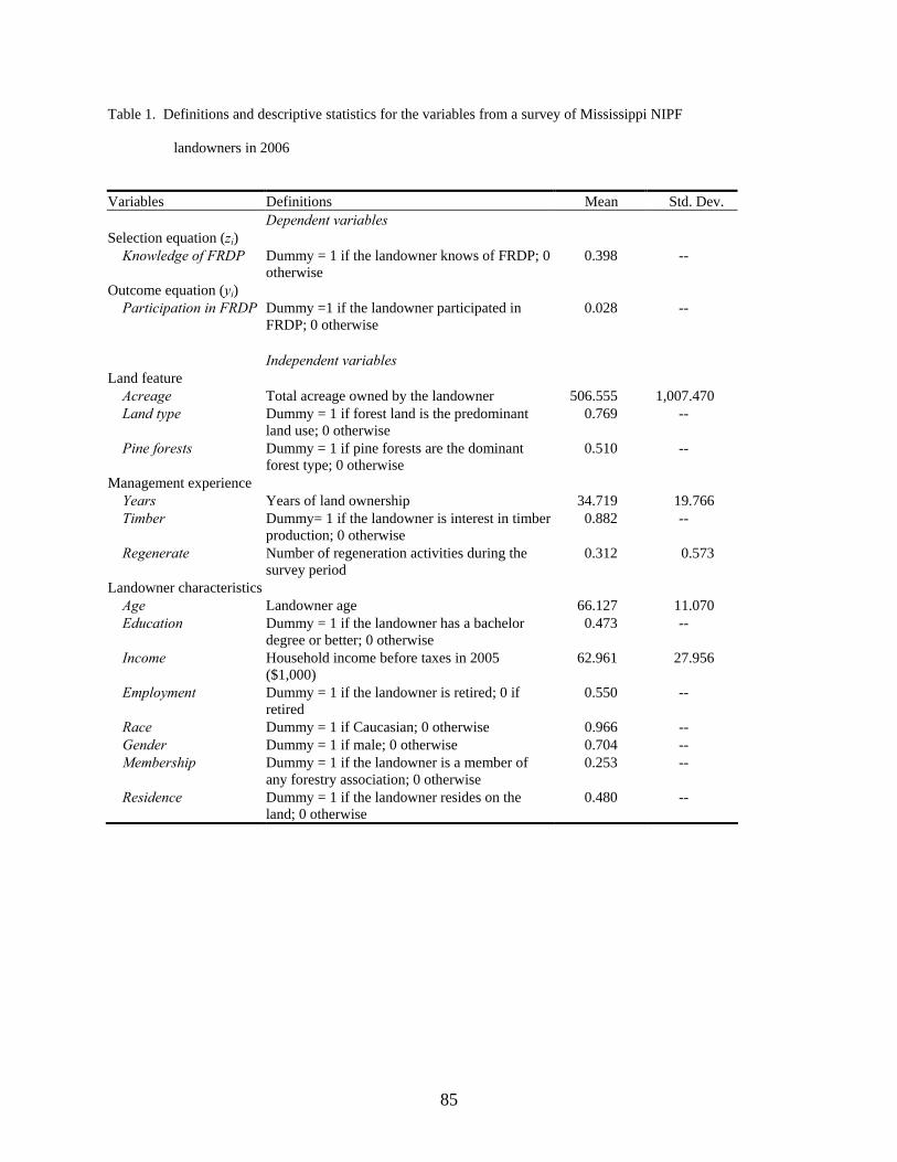
85

Table 1. Definitions and descriptive statistics for the variables from a survey of Mississippi NIPF

landowners in 2006

Variables Definitions Mean Std. Dev. Dependent variables Selection equation (zi) Knowledge of FRDP Dummy = 1 if the landowner knows of FRDP; 0

otherwise 0.398 --

Outcome equation (yi) Participation in FRDP Dummy =1 if the landowner participated in

FRDP; 0 otherwise 0.028 --

Independent variables Land feature Acreage Total acreage owned by the landowner 506.555 1,007.470 Land type Dummy = 1 if forest land is the predominant

land use; 0 otherwise 0.769 --

Pine forests Dummy = 1 if pine forests are the dominant forest type; 0 otherwise

0.510 --

Management experience Years Years of land ownership 34.719 19.766 Timber Dummy= 1 if the landowner is interest in timber

production; 0 otherwise 0.882 --

Regenerate Number of regeneration activities during the survey period

0.312 0.573

Landowner characteristics Age Landowner age 66.127 11.070 Education Dummy = 1 if the landowner has a bachelor

degree or better; 0 otherwise 0.473 --

Income Household income before taxes in 2005 ($1,000)

62.961 27.956

Employment Dummy = 1 if the landowner is retired; 0 if retired

0.550 --

Race Dummy = 1 if Caucasian; 0 otherwise 0.966 -- Gender Dummy = 1 if male; 0 otherwise 0.704 -- Membership Dummy = 1 if the landowner is a member of

any forestry association; 0 otherwise 0.253 --

Residence Dummy = 1 if the landowner resides on the land; 0 otherwise

0.480 --

86

Table 2. Results of NIPF landowner knowledge of and participation in Mississippi Forest Resource

Development Program (FRDP)

Outcome equation

Selection equation (Unrestricted) (Restricted)

Coeffi. (t-ratio)

Marginal Effect

Coeffi. (t-ratio)

Coeffi. (t-ratio)

Marginal Effect

Constant -0.809*** (-2.900)

-0.312 -0.791 (-0.469)

-1.455*** (-3.322)

-0.054

Land features Acreage 1.183E-4***

(3.081) 4.553E-5 1.603E-4

(0.560) --

--

Land type -0.012 (-0.172)

-0.004 -0.029 (-0.135)

-0.023 (-0.159)

-0.003

Pine forests -0.020 (-0.363)

-0.008 -0.186 (-0.957)

--

--

Management experience Years 0.001

(0.629) 3.779E-4 0.002

(0.309) 0.001

(0.210) 2.563E-5

Timber 0.200** (2.204)

0.075 0.430 (0.700)

0.126 (0.532)

0.013

Regenerate 0.068 (1.389)

0.026 0.967***(3.576)

0.850*** (6.796)

0.032

Landowner characteristics Age -0.005

(-1.485) -0.002 -0.005

(-0.274) --

--

Education 0.113* (1.888)

0.044 0.428 (1.143)

0.251* (1.672)

0.029

Income -0.001 (-0.615)

-2.623E-4 -0.001 (-0.273)

1.447E-4 (0.061)

5.385E-6

Employment 0.174** (2.445)

0.067 0.351 (0.632)

0.131 (0.882)

0.015

Race 0.119 (0.761)

0.045 0.032 (0.062)

-0.167 (-0.571)

-0.021

Gender 0.279*** (4.463)

0.105 0.790 (0.948)

0.385* (1.688)

0.039

Membership 0.533*** (8.299)

0.208 1.576 (0.989)

0.751** (1.985)

0.115

Residence 0.101* (1.748)

0.039 0.370 (1.057)

0.221 (1.515)

0.025

P1V -- -6.780 (-0.882)

-2.807* (-1.642)

-0.104

Log Likelihood

-1,421.979 -201.769 -203.211

Chi-squared 153.384 170.003 167.118 Observation 2,229 2,229 2,229 ***, **, and * indicate significance at the 1%, 5%, and 10%, respectively.

87

How Long Do NIPF Landowners Wait to Reforest after Harvesting?*

Xing Sun1, Ian A. Munn2, Changyou Sun3, and Anwar Hussain4 Abstract: Understanding how quickly landowners regenerate their timberlands after harvest is critical to developing policies to improve forest productivity. Using survey data from 81 counties in Mississippi from 1996 to 2006, this study investigated the length of the time interval between harvest and reforestation. Non-parametric duration analysis was used to examine how long NIPF landowners waited to reforest after harvesting. The average time that elapsed from harvest to regeneration was 11 months within the study period. The probability of regeneration reached its highest value in the 16th month after harvest and thereafter decreased steadily until the 28th month, after which the probability of regeneration was essentially nil. Keywords: Duration analysis, non-industrial forest landowners, reforestation delay Introduction

Reforestation is essential for maintaining productive timberlands. Replanting trees on productive timberlands after harvesting is an effective way to increase the commercial value to non-industrial private forest (NIPF) landowners. Landowners benefit not only financially from higher timber production, but also from more attractive aesthetic landscapes with clear water and enhanced wildlife habitat. However, nearly half (48.5%) of Mississippi NIPF landowners do not reforest their timber following a harvest (Gunter et al. 2001). Timely reforestation is even more important for both timber production and environmental protection. Not replanting after harvesting or delayed replanting may affect timber supply and reduce non-timber outputs and benefits (e.g., clear air and water, soil, wildlife). Softwood removals exceeded growth by approximately 18% in Mississippi in 2002 (Smith et al. 2004). This will impact future timber markets. In addition, if the lands are not replanted for a prolonged period of time, water and soil values on the harvested lands may deteriorate and wildlife habitat may degrade. Therefore, time elapsed from harvest to reforestation is a critical indicator of good forest resource management.

* This manuscript is publication #FO353 of the Forest and Wildlife Research Center, Mississippi State University. 1 Graduate Research Assistant, Department of Forestry, Mississippi State University, Box 9681, Mississippi State, MS 39762, xs31@msstate.edu, (662) 325-5812 (v), (662) 325-8726 (fax). 2 Professor, Department of Forestry, Mississippi State University, Box 9681, Mississippi State, MS 39762, imunn@cfr.msstate.edu, (662) 325-4546 (v), (662) 325-8726 (fax). 3 Assistant Professor, Department of Forestry, Mississippi State University, Box 9681, Mississippi State, MS 39762, csun@cfr.msstate.edu, (662) 325-7271 (v), (662) 325-8726 (fax). 4 Assistant Research Professor, Department of Forestry, Mississippi State University, Box 9681, Mississippi State, MS 39762, ahussain@cfr.msstat.edu, (662) 325-4259 (v), (662) 325-8726 (fax).

88

A number of empirical studies have investigated the impact of various factors such as characteristics of landowners, land, and forest management on landowner reforestation decisions (Amacher et al. 2003). However, none has considered the time dimension of reforestation. How long NIPF landowners wait to reforest after harvesting is an important but unanswered question. The answers to this question would be useful in formulating policies to help landowners reforest in a timely manner after harvesting. Many empirical studies have examined NIPF landowner regeneration. Typically, regeneration studies have relied on a binary choice model (Hyberg and Holthausen 1989; Royer 1987). The typical dependent variable was a binary variable indicating regeneration or no regeneration. Independent variables included land characteristics (e.g., acreage, land type), owner demographics (e.g., income, education, residence), and market factors (e.g., sawtimber price, pulpwood price, reforestation cost). Royer (1987) used a logistic regression model to estimate the probability of reforestation by southern landowners who had conducted final harvests on 10 or more acres between 1971 and 1981 in 12 southern states. Income, reforestation costs, government cost-sharing, technical assistance, and pulpwood price were highly important determinants of reforestation. Hyberg and Holthausen (1989) also used logistic regression to investigate the harvest timing and reforestation investment decisions of private landowners and obtained similar results. More recently, Zhang and Flick (2001) used a two-step selectivity model and determined that income and government financial assistance programs increased the probability of reforestation. Gunter et al. (2001) determined useful factors for predicting reforestation by NIPF landowners in Mississippi. Landowners more likely to regenerate were those with large ownerships, higher income levels, better education, work in professional or business occupations, white males, and living in larger cities (Gunter et al. 2001). Beach et al. (2005) showed that both tract size and timber prices had a significant positive effect on reforestation, and among the owner characteristics, income influenced reforestation. Earlier studies explored NIPF landowner reforestation behavior using qualitative response models and identified relevant variables. However, previous research has not explored the time elapsed before regeneration. This research focused on the interval between harvesting and regeneration by NIPF landowners in Mississippi, a typical southern state where timber plays an important role in the state economy and most of the timberland is owned by NIPF landowners. The objective of this study was to examine how long NIPF landowners waited to reforest after harvesting. Non-parametric duration analysis was employed to examine the time elapsed to regenerate after harvesting.

Conceptual Framework and Survey Data

Analytical Framework

This research used cross-sectional survey data from Mississippi to examine timely regeneration. The survey period covered ten years from 1996 to 2006. Duration analysis was employed to examine the time interval between finishing harvest and beginning reforestation. Duration analysis is a class of statistical methods for studying the occurrence and timing of events (Allison

89

1995; Greene 2003). The focal variable was the time to regenerate, T , measured as the time between the completion of harvest and the occurrence of regeneration. The event of interest in this study was whether NIPF landowners reforest their harvested timberland within the study period, which is indicated by an additional variable Status (Status = 1 if regeneration occurred within the study period; Status = 0 if not). If an individual did not regenerate within the study period, the observation was censored in the sense that the duration before regeneration was at least the observed interval. Estimation needs to account for the censored nature of the data.

Survey and Sample

The Social Science Research Center at Mississippi State University conducted a phone survey during July and August of 2006. The survey sample was drawn from a database of landowner records in Mississippi. The database covered 81 of the 82 counties in Mississippi. The records for Hinds County were not available. Since NIPF landowners were the focus of this study, companies and partnerships were excluded. In addition, only NIPF owners with at least 100 acres of land were selected in order to eliminate small landowners with infrequent forest management activities. That yielded a list of about 20,000 owners. Landowner phone numbers were provided by a commercial service. Finally, among landowners with phone numbers, a random sample of 9,925 landowners was selected and used in the phone survey. During the phone survey, several questions were asked to select landowners relevant for the study objectives. If the landowner owned less than 100 acres or did not harvest during the study period, the phone interview was stopped. Also, landowners who carried out a thinning or a selection cut were excluded. Furthermore, T was measured by the time interval between finishing harvest and beginning regeneration. Landowners who harvested and regenerated within the study period, but could not recall either the harvest date or regeneration date were deleted. If the landowner provided only the season and not an exact month, the mid point of the season was used (i.e., March for Spring, June for Summer, September for Fall, and December for Winter). Methodology Non-parametric analysis was employed to analyze the relation between the length of the interval and the time of beginning regeneration (Allison 1995). Non-parametric techniques were used to compute the time elapsed between completion of harvest and beginning of regeneration and plot regeneration and non-regeneration probability. Two non-parametric methods were employed: Kaplan-Meier Product Limit method and Life Table method. The Kaplan-Meier estimation was used to obtain exact non-regeneration probability and the time interval between harvest and regeneration. The function of time elapsed before regeneration and hazard function were estimated with the Life-Table method. The time interval between completion of harvest and beginning of regeneration, T, is expressed as follows:

(1) T f x= ( ) where T was treated as a random variable.

90

There are four equivalent ways to describe the continuous probability distribution for T. The probability density function (p.d.f.) denoted as ( )f t and the cumulative distribution function (c.d.f.) denoted as ( )F t are used to estimate parameters of this model. T ’s probability density function (p.d.f.) and cumulative distribution function (c.d.f.) are mathematically expressed as:

(2) f t dF tdt

t T t ttt

( ) ( ) lim Pr( )= =

≤ < +→∆

∆∆0

(3) ( ) ( ) ( )dxxftTtFt

∫≤=0

Pr .

Equation (3) illustrates the probability that T will be less than or equal to any t value that we examined. In addition to these two functions, the function of time elapsed before regeneration ( )S t and hazard function ( )h t are commonly used in the duration analysis relevant to the timely

regeneration. The function of time elapsed before regeneration ( )S t is an unconditional probability distribution and is defined as the probability that the interval between harvesting and regenerating will be greater than t. It is expressed mathematically as follows:

(4) ( ) ( ) ( ) ( )dxxftFtTtSt∫∞

=−=>= 1Pr .

In this study, this function estimates the probability of non-reforestation beyond any time t. ( )S t reaches the maximum probability when t equals 0. Hazard function ( )h t is a conditional density distribution and represents the instantaneous rate of reforestation at time t, given that the harvested timberland has not been reforested up to t. This function is a popular and useful way of describing T distribution in duration analysis (Allison 1995). Its mathematical equation is defined as follows:

(5) ( ) ( ) ( )( )tStf

ttTttTtth =

∆≥∆+<≤

=|Prlim .

Equation (5) illustrates the probability that a regeneration event occurs in the small interval between t and t t+ ∆ conditional on T≥ t. The functions, ( )f t and ( )F t , are used for parameter estimation while ( )S t and ( )h t are used to answer research questions.

Empirical Results Survey Results

Of the 9,925 landowners contacted by phone, 2,126 owned less than 100 acres, and 2,132 did not harvest timber in the past 10 years. Consequently, these landowners were excluded from the survey. There were also 1,110 wrong phone numbers. Other reasons for unsuccessful calls

91

included communication problems, refusal to participate, and deceased owners. Hence, there were 2,229 landowners who completed the survey.

There were 1,081 final harvests conducted by these 2,229 landowners. Of these, 695 were replanted by the end of the study period and 386 were not. Of the 695 respondents replanting, 264 did not recall either the harvest date nor regeneration date, whereas another 36 recalled that the harvest date took place later than the regeneration date, which is not feasible, so these observations were excluded from the data analysis. Of the 386 respondents who had not replanted after harvest, 121 of them did not recall the harvest date and another 5 recalled the harvest date not taking place during the survey period. Hence, these observations were also excluded from the data analysis. After accounting for invalid observations and non-responses, 655 observations were available for statistical analysis. The completion rate was 60.6%. For 395 observations, landowners harvested and then regenerated timberland within the study period, whereas for 260 observations, landowners harvested but did not regenerate by the end of study.

Non-Parametric Duration Analysis Non-parametric duration analysis estimated the time interval between the completion of the harvest and the beginning of regeneration with an additional consideration: regeneration or no regeneration. The average time elapsed before regeneration (T) was 11 months for harvests that were regenerated within the study period (n = 395). The average time elapsed before regeneration (T) was 44 months for harvests regardless of whether regeneration occurred during the study period for all observations (n = 655). The probability that a harvested site was not regenerated at time t is shown in Figure 1. This figure depicts the survivor function S(t) at time ti, the probability of non-regeneration following harvest when the waiting time is greater than ti. The probability that the landowner had not regenerated after harvest declined as the length of time from completion of the harvest increased. The reduction in the rate sharply decreased until the 25th month. The probability that the tract has not been regenerated after harvest decreased rapidly during the first 25 months, then leveled off. The probability distribution of estimated hazard function is shown in Figure 2. This figure depicts that the hazard function ( )h t at time ti , the probability of regeneration at a given time following harvest. This probability reached its highest value in the 16th month and decreased thereafter rapidly until the 28th month. In the 28th month, the probability of regeneration was approximately 0.6% and remained less than 1% as the time increased. Along this prediction track, the probability of regeneration approaches zero as the time since harvest increases. Conclusions This study surveyed Mississippi NIPF landowners to address timely regeneration of harvested lands. Non-parametric duration analysis was used. The analysis yielded more insightful results in terms of timely regeneration than a simple logistic regression model. Furthermore, this study

92

is the first attempt to use duration analysis to examine effects of various factors on the time interval associated with reforestation decision. The survey revealed that about 40% NIPF landowners in Mississippi did not replant their harvested timberland in past ten years. On average, NIPF landowners that replanted waited 11 months to regenerate after harvest. After the 16th month following harvest, the probability of regeneration decreased until 28th month. These results need to be qualified by several considerations. First, non-parametric techniques, as the name suggests, drop the formal modeling framework (Greene 2003). Furthermore, they do not consider the impact of other variables on the dependent variable. Therefore, non-parametric duration analysis is the most general of the techniques, but, consequently, the least precise. So, semi-parametric and parametric analyses need to be used to further provide more precise characterization of the relationship between the time interval from harvest to regeneration and various variables influencing the regeneration interval. Second, the intent of this study targets the timely regeneration behavior after harvesting. However, this is just one of several landowner behaviors; other would include the timely harvest behavior and other forestry management practices to provide a more comprehensive look at the landowner behavior.

Literature Cited Allison, P.D. (1995). Survival Analysis Using SAS: A practical guide. Cary, North Carolina. SAS

Publishing.

Amacher, G.S., M.C. Conway, and J. Sullivan (2003). Econometric analyses of nonindustrial forest landowners: is there anything left to study? Journal of Forest Economics 9(2):137-164.

Beach, R.H., S.K. Pattanayak, J.C. Yang, and B.C. Muray (2005). Econometric studies of non-industrial private forest management: a review and synthesis. Forest Policy and Economics 7(3):261-281.

Greene, W.H. (2003). Econometric Analysis. Pearson Education, Inc., Delhi, India.

Gunter, J.E., S.H. Bullard, M.L. Doolittle, and K.G. Arano (2001). Reforestation of harvested timberlands in Mississippi: behavior and attitudes of non-industrial private forest landowners. FWRC Research Bulletin # FO 172, Forest and Wildlife Research Center, Mississippi State University. 25p.

Hyberg, B.T., and D.M. Holthausen (1989). The behavior of non-industrial private forest landowners. Canadian Journal of Forest Research 19:1014–1023.

Royer, J.P. (1987). Determinants of reforestation behavior among southern landowners. Forest Science 33(3):654-667.

Smith, W.B., P.D. Miles, J.S. Vissage, and S.A. Pugh (2004). Forest resources of the United States 2002. USDA Forest Service Gen. Tech. Rep. NC-241.

Zhang, D., and W.A. Flick (2001). Sticks, carrots, and reforestation investment. Land Economics 77(3):443-456.

93

0%

10%

20%

30%

40%

50%

60%

70%

80%

90%

100%

0 8 16 24 32 40 48 56 64 72 80 88 96 104

112

120

128

Months after completion of the final harvest

Prob

abili

ty o

f non

-reg

erne

ratio

n n

Figure 1. Survival function for regeneration of harvested forest land by Mississippi nonindustrial private forest landowners from 1996 to 2006.

94

0%

1%

2%

3%

4%

5%

6%

7%

1 7 13 19 25 31 37 43 49 55 61 67 73 79 85 91 97 103

109

115

121

127

Months after completion of the final harvest

Prob

abili

ty o

f reg

ener

atio

n n

Figure 2. Hazard function for regeneration of harvested forest land by Mississippi nonindustrial private forest landowners from 1996 to 2006.

95

Analysis of Family Forest Holdings Structure in the United States

Yaoqi Zhang1, Xianchun Liao2, and Brett J. Butler3

Abstract: This paper is aimed to address why increasing share as well as the number of small-scale family forest owners using economic theory as well as the data. We examined the state-level structure of the size of family forest holdings in the conterminous United States based on data collected by the USDA Forest Service, National Woodland Owner Survey in 1993 and 2003, and using seemingly unrelated regression. Keywords: Non-industrial private forest, family forest, seemingly unrelated regression, National Woodland Owner survey Introduction Currently, there are an estimated 248 million hectares of forestland in the conterminous United States (Smith et al 2004). Nearly two-thirds, or 157 million hectares, are privately owned and two-thirds of the private forestland, 105 million hectares, are owned by 10.3 million families and individuals (Butler and Leatherberry 2004). The number of family forest owners varies significantly across the country. The North has 46% of the family forest owners in the United States, the South has 42%, and the West has only 12 %. Family forest owners have been changing dynamically. The number of family forest owners in the contiguous U.S. increased from 9.3 million in 1993 to 10.3 million in 2003. Research also suggests that the share or even the total acreage owned by small owners (less than 20 hectares) has significantly increased in the past 10 years (Butler and Leatherberry 2004). DeCoster (1998) stated that, if the trend continues, by the year 2010 nearly 95 percent of the national private forestlands will be owned by individuals with less than 40 hectares. It is widely believed that, in the U.S., average holding size of family forest owners is shrinking through a process called parcellation. So far, more claims than concrete evidence have been made. Because transition probability matrices that include transfers from other ownership types (e.g., forest industry, NIPF) and loss of forest land (e.g., to development) are not available, analyzing parcellation for family forest owners in the United States is very challenging. As an alternative that we use in this study, we examined the structural differences of sizes of family forest holdings among states. Even though the differences among the states are not the same as the

* The work on this paper was financially supported by the McIntire-Stennis program of USDA (project #: ALAZ00032), Southern Research Station of USDA Forest Service. We appreciate comments and suggestions from Dr. Indrajit Majumdar. All errors are responsibilities of the authors. 1 School of Forestry and Wildlife Sciences, Auburn University, AL 36849, Yaoqi.Zhang@auburn.edu, (334) 844-1041 (v), (334) 844-1084 (fax). 2 School of Forestry and Wildlife Sciences, Auburn University, AL 36849, liaoxia@auburn.edu, (334) 844-8042 (v), (334) 844-1084 (fax). 3 USDA Forest Service, Northern Research Station, Holdsworth Hall, Amherst, MA 01003, bbutler01@fs.fed.us, (413) 545-1387 (v), (413) 545-1860 (fax).

96

intra-state trends, the findings can explain the variation across states, and can shed light on the changes and the associated factors. Methodology Fundamentally, small-scale forestry is associated with issues of significant transaction costs of environmental services (Zhang et al 2005). Alternatively, it is also an issue of in-house production or by a market like silviculture in the forestry sector (see Wang and Van Kooten 2000). Small scale forestry is largely for transaction cost savings (Zhang 2001). Economics tells us that optimal holding size is when the net marginal utility is equal to the marginal cost, or simply the market price of forestland plus holding costs (e.g., taxes, management, and risk.) Owners might adjust their holding sizes in response to the change in input and output price. Therefore, the structural changes in holding sizes are equal to the aggregated responses to the changes in demographic and economic factors, such as the population and per capita income. For small land owners, almost all previous studies have indicated that their objectives have been shifting from timber to non-timber. We can see such trends not only from survey of their motivation, but also from their forest management practice in terms of species, rotation. For example, small family owners tend to plant hard woods and have longer rotation, or simple less likely harvest the timber. In contrast, if the primary ownership objective is timber production, the holding size should be based primarily on the efficiency of timber production . Holding size tends to be larger because of technological advance that is in favor of larger scale in forestland management and ownership. Of course the ultimate choice of the size of forest holdings will be mitigated by capital and land availability. Socio-economic and biophysical conditions determine the forest management objective as well as the timber and non-timber values. Therefore, there should be observable relationships between the structure of forestland holding sizes and the socio-economic and bio-physical characteristics of the forest land and the forest land owners. Following Mehmood and Zhang (2001) and Pan (2006), we conduct an empirical analysis. We assume that holding size is a function of a group of variables representing the factors determining the holding size. The holding size structure is determined by the marginal costs and values of the inputs and outputs. First, we hypothesize that population density is an important factor since more forest and agricultural land need to be converted to residential and commercial uses as population increases (Nagubadi and Zhang 2005), and therefore population density impacts demand and price for forestland. Changes to the spatial distribution of people, such as urbanization, will also impact the structure of forest holding sizes. People living in cities, suburbs, or urban/rural interfaces have different expectations for their lands than rural people and are more likely to own land as part of their home site or recreation and less likely to have timber production as a major motivation. Demographics and economic factors may be associated with the changes in the holding size as well (Gobster and Rickenbach 2003). For example, an aging population might be an indication of more land transfers, subsequent parcellation, and consequently an increase in the number of smaller holdings. Income that affects the utility function and owners’ demands for different

97

mixes of products and services from their forestland is also likely to influence the structure of the forest holding sizes. As income increases, to live in or around the woods seems to be a growing lifestyle trend (DeCoster 1998). The Gini index quantifies income disparity (Volscho 2004) and may be a significant predictor of parcellation and consolidation (Sisock 1998; Pan 2006). Private forestland availability may also affect the average holding size, and might affect holding size structure. To put all these variables together, the empirical specification of our models is as follows:

im PFPGINIINCPURBANOLDPPOPDY 1161514131211 εββββββα +++++++= (1)

iiiiiiiii PFPGINIINCPURBANOLDPPOPDY εββββββα +++++++= 654321 (2) where Ym is the mean holding size in a state; Yi is the percentage of family forestland in holdings between 1 and 19 hectares (small), the percent of forestland in holdings between 20 and 199 hectares (medium), and the percentage of forestland in holdings 200 hectares or larger (large); POPD is population density per square mile; OLDP is the percentage of the population who are 65 years of age or older; URBAN is the percent of the population living in urban areas; INCP is per capita income; GINI is the Gini index for income disparity; and PFP is per capita private forestland. The units and data sources for these variables are listed on Table 1. The equation (1) with average holding size is viewed as a contrast to equation (2). Ordinary least square (OLS) is used to estimate the first equation . The multiple equations (2) are estimated jointly as a seemingly unrelated regression (SUR) model (Zellner 1962; Thei 1971) because the explanatory variables that affect the share of holding size are the same for the three models (small, medium, and large). This method allows individual shares of forestland and residual variances to differ across the models. The advantage of this approach over residual analysis is to test the joint hypotheses since the heteroscedasticity across equations is explicitly incorporated in the statistical tests (Binder 1985; Theil 1971, chapter 7). Both level and log transformation are explored for these equations. Data A unique data source that can be used is the data collected in 1993 and 2002-2004, henceforth referred to as 2003, as part of the National Woodland Owner Surveys (NWOS) conducted by the USDA Forest Service’s Forest Inventory and Analysis program (Birch 1996; Butler et al 2005). In this study, we exclude data from the 1978 national study of private forest owners (Birch et al 1982) statistics because no data on size of forest holdings specifically for family forest owners were reported – most of the data were for all private owners, including industrial forest owners. The NWOS is the nation’s census of forest owners. On a recurring basis, it contacts a random set of forest owners across the United States to ascertain information about their forestland, ownership objectives, forest use, forest management practices, sources of information, concerns and issues, and demographics.

98

Table 1. Description of variables and data sources Variables Description Data sources

MEAN Average holding size National Woodland Owner Surveys (Birch 1996; Butler et al. 2005)

SMALL Percent of forestland in holding size less than 20 hectares (%)

National Woodland Owner Surveys (Birch 1996; Butler et al. 2005)

MEDIUM Percent of forestland in holding size between 20 and 200 hectares (%)

National Woodland Owner Surveys (Birch 1996; Butler et al. 2005)

LARGE Percent of forestland in holding size larger than 200 hectares (%)

National Woodland Owner Surveys (Birch 1996; Butler et al. 2005)

POPD Persons per square mile U.S. Census Bureau 2000 and 1990

OLDP Persons 65 years old and over U.S. Census Bureau 2000 and 1990

URBAN Percent of urban population U.S. Census Bureau 2000 and 1990

PFP Per capita private forestland (hectares) Forest Resources of the United States 2002 (Smith et al. 2004)

INCP Per capita income ($1,000) U.S. Census Bureau 2000 and 1990

GINI Gini index of family income Volscho (2004)

At a random set of sample points across the United States, the NWOS uses remotely sensed imagery to determine if sample points are forested. For the forested points, ownership information is collected from tax offices or other public sources. This information is used to contact the forest owners using a mixed-method survey; a self-administered mail survey is the primary data collection method and telephone interviews are used to increase response rates. Detailed information on data collection and processing procedures are described in Butler et al (2005). Our data set had 92 observations (four states Hawaii, Nevada, Alaska, and Idaho were excluded from our data set due to missing data) for 46 states and two points in time – 1993 and 2003. Table 1 describes the dependent and independent variables and data sources. For each state, landowners were categorized into six size classes: less than 4, 4-19, 20-39, 40-199, 200-399, and more than 400 hectares. Means were calculated as the weighted average size (see Mehmood and Zhang 2001).

99

We broke down the forestland holdings into three groups based on previous research, data availability, and the objective of approximately equal distribution of the sample among the groups. 20 hectares is a common threshold below which many experts feel timber production is not commercially viable or is, at least, at a competitive disadvantage and less likely to be a major ownership objective. Therefore, the percent of forestland in holdings of less than 20 hectares was used to indicate owners with smaller holdings and, presumably, non-timber ownership objectives. An increase in the percentage of forestland in this group is considered an indicator of forest parcellation. The group with owners with holdings between 20 and 199 hectares was labeled medium, the group with owners of holdings of 200 hectares or more was labeled large. The specific break points are arbitrary, but we believe they are an appropriate approximation for measuring the structure of the family forestland holdings. Socio-economic data such as POPD, OLDP, URBAN, INCP were obtained from the U.S. Census Bureau for 2000 and 1990 (Insert reference). Data for the GINI index on income disparity was calculated by Volscho (2004). Per capita private forestland area is a proxy for private forestland availability and was obtained from Forest Resources of the United States 2002 (Smith et al 2004). Results The Variation of Family Forestland Holdings The average holding size and percent of small-scale forest owners measured by less than 20 hectares (the other two groups are: between 20 and 199 hectares, and large than 200 hectares). Across states, the mean holding size in the South is larger than in the North and the West. About 90 percent of the family forest owners in the United States own less than 20 hectares each and, in total, own one third of the family forestland. About 10 percent of the family owners own 20 hectares or more and, in total, own two thirds of the family forestland. On average, the holding sizes are smallest in the North (11 hectares) followed by the West (14 hectares) and the South (21 hectares). From 1993 to 2003, the average size of family forest holdings remained almost constant (decreased by 1 percent), but the share of small and large holdings increased by 4 percent and 13 percent, respectively, while the medium sized holdings decreased by 8 percent. This is consistent with the argument made by Zhang et al. (2005) and the finding by Ripatti (1996). If we just see the average holding size we would not see such change in structure. The Factors Associated with the Holding Size Structure Table 2 presents the results of our regressions by OLS (for mean) and SUR model (for the share). The impacts of different variables can be compared to each other effectively since the coefficients have an interpretation as the elasticity of a log-form model. Overall, the explanatory variables significantly explain the four dependent variables measuring forestland holding structure (R2 values between 0.40 and 0.61). All of the independent variables showed the expected relationship with the dependent variables.

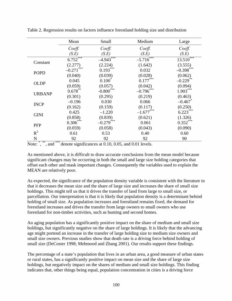
100

Table 2. Regression results on factors influence forestland holding size and distribution

Mean Small Medium Large

Coeff. (S.E)

Coeff. (S.E)

Coeff. (S.E)

Coeff. (S.E)

Constant 6.752*** (2.277)

–4.943*** (2.224)

–5.716*** (1.642)

13.510*** (3.555)

POPD –0.271*** (0.040)

0.193*** (0.039)

0.032 (0.028)

–0.398*** (0.062)

OLDP 0.045 (0.059)

0.100* (0.057)

0.177*** (0.042)

–0.229** (0.094)

URBANP 0.678** (0.301)

-0.800*** (0.295)

–0.796*** (0.219)

1.903*** (0.463)

INCP –0.196 (0.162)

0.030 (0.159)

0.066 (0.117)

–0.467* (0.250)

GINI 0.425 (0.858)

–1.220 (0.839)

–1.677*** (0.621)

6.223*** (1.326)

PFP 0.306*** (0.059)

–0.279*** (0.058)

0.061 (0.043)

0.352*** (0.090)

R2 0.61 0.53 0.40 0.60 N 92 92 92 90

Note: *, **, and *** denote significances at 0.10, 0.05, and 0.01 levels. As mentioned above, it is difficult to draw accurate conclusions from the mean model because significant changes may be occurring in both the small and large size holding categories that offset each other and mask important changes. Consequently the variables used to explain the MEAN are relatively poor. As expected, the significance of the population density variable is consistent with the literature in that it decreases the mean size and the share of large size and increases the share of small size holdings. This might tell us that it drives the transfer of land from large to small size, or parcellation. Our interpretation is that it is likely that population density is a determinant behind holding of small size. As population increases and forestland remains fixed, the demand for forestland increases and drives the transfer from large owners to small owners who use forestland for non-timber activities, such as hunting and second homes. An aging population has a significantly positive impact on the share of medium and small size holdings, but significantly negative on the share of large holdings. It is likely that the advancing age might portend an increase in the transfer of large holding size to medium size owners and small size owners. Previous studies show that death rate is a driving force behind holding of small size (DeCoster 1998; Mehmood and Zhang 2001). Our results support these findings. The percentage of a state’s population that lives in an urban area, a good measure of urban states or rural states, has a significantly positive impact on mean size and the share of large size holdings, but negatively impact on the shares of medium and small size holdings. This finding indicates that, other things being equal, population concentration in cities is a driving force

101

behind holding of large size of forestland. This finding contradicts findings from pervious studies (Befort et al 1998; Mehmood and Zhang 2001). Our results indicate that as the percentage of urban population increases or in more urbanized states, the mean holding size decreases. Although urbanization influences changes in land use patterns near cities, remaining people in the rural area are more likely own larger forestland as more people move to cities. The impression of most people on the impact of urbanization on the parcellation might be wrong since it does not exclude the impact by total population growth and without considering the variation spatially. Holding all other variables equal, the rural population is still more likely to own forestland, which suggests that the rural population could cause mean holding size to decrease. The income per capita has a significantly negative impact on the share of large size holdings, which is in agreement with the literature (Mehmood and Zhang 2001). The estimate for the income variable indicates that as income increases, people devote more money to non-timber production. However, the result should be considered with caution; the shares of medium and small holdings show the expected signs, but neither of the coefficients is statistically significant. It is interesting to observe that the income distribution, which is measured by the Gini Index, has a significantly positive impact on the share of large size holdings, but a significantly negative impact on the share of medium size holdings. It implies that income variation is a driving force behind holding of large size. A plausible interpretation is that less equal income distribution states have smaller shares of small and medium holdings, but increase the share in large size. The results should be considered with caution because it has no significantly negative impact on small holding of forestland. Theoretically, a negative impact on small holding size should have a positive impact on large holding size. Not surprisingly, per capita private forestland had significantly positive impacts on mean and share of large holdings, but a negative impact on the share of small holdings, and a positive, but statistically non-significant, impact on the share of medium size holdings. This finding suggests that per capita forestland is a driving force behind holding of large size. A possible explanation is that as private forestland is more available, the possibility of larger parcels is higher. Literature Cited Befort, W.A., A.E. Luloff, and M. Morrone. 1988. Rural land use and demographic change in a

rapidly urbanizing environment. Landscape and Urban Planning 16:345-56 Binder, J.J. 1985. Measuring the effects of regulation with stock price data. Rand Journal of

Economics 16(2): 167-183. Birch, T.W. 1996. Private forestland owners of the United States, 1994. USDA For. Serv.

Northeast For. Exp. Stat. Resour. Bull. NE-138. 195 p. Birch, T.W., D.G. Lewis, H.F. Kaiser. 1982. The private forest-land owners of the united states.

U.S. Department of Agriculture, Forest Service. Resour. Bull. WO-1. 64 p.

102

Bliss, J.C., M. L. Sisock, T.W. Birch. 1998. Ownership matters: forestland concentration in rural Alabama. Society and Natural Resources: 11 (4): 401-410.

Butler, B.J., E.C. Leatherberry, M.S. Williams. 2005. Design, implementation, and analysis

methods for the National Woodland Owner Survey. U.S. Department of Agriculture, Forest Service, Northeastern Research Station, Newtown Square, PA. Gen. Tech. Rep. NE-GTR-336. P. 43.

Butler, B.J., E.C. Leatherberry. 2004. America’s family forest owners. Journal of Forestry 102

(7): 4-14. Decoster, L.A. 1998. The boom in forest owners—A bust for forestry? Journal of Forestry

96(5):25-28. Gobster, P. H., M.G. Rickenbach. 2003. Private forestland parcelization and development in

Wisconsin’s Northwoods: perceptions of resource-oriented stakeholders. Landscape and Urban Planning 69: 165-182.

Hartsell, A.J., M. J. Brown. 2002. Forest Statistics for Alabama, 2000. Resource Bulletin SRS-

67. USDA Southern Research Station. Larson, K. 2004. Family forests—the bigger picture. Journal of Forestry (Oct./Nov. 2004):13-14. Mehmood, S.R., D. Zhang. 2001. Forest Parcelization in the United States. Journal of Forestry

99(4): 30-34. Nagubadi, R.V., D. Zhang. 2005. Determinants of timberland use by ownership and forest type

in Alabama and Georgia. Journal of Agricultural and Applied Economics 37(1):173-186. Pan, Y. 2006. Analysis of Holding Size Distribution of private Forestland Ownership. Master

Thesis, Auburn University. USA. Ripatti, P. 1996. Factors Affecting Partitioning of Private Forest Holdings in Finland: A Logit

Analysis. Acta Forestalia Fennica 252. Rosen, J.F., L. Doolittle. 1987. Profiles of Midsouth Non-industrial private forests and owners.

Resource Bulletin. SO-125. New Orleans, LA: United States Department of Agricultural, Forest Service, Southern Forest Experiment Station.

Sisock, M.L. 1998. Unequal shares: forest land concentration and well-being in the rural

Alabama. Master Thesis, Auburn University. USA. Smith, W.B., P.D. Miles, J.S. Vissage. 2004. Forest resources of the United States, 2002. U.S.

Department of Agriculture, Forest Service, North Central Research Station, St. Paul, MN. Gen. Tech. Rep. NC-241. 137 pp.

Theil, H. 1971. Principles of Econometrics. NY: John Wiley and Sons.

103

US Census Bureau (2000). Census 2000 Data for the United States

http://factfinder.census.gov/servlet. Cited 1 Aug 2006 US Census Bureau (1990). Census 1990 Data for the United States

http://factfinder.census.gov/servlet. Cited 1 Aug 2006 Volscho, T.W. 2004. Gini Index of Family Income by U.S. County, 2000. University of

Connecticut, Dept of Sociology: http://vm.uconn.edu/~twv00001/counties.htm. Cited 15 July 2006.

Wang, S., G.C. van Kooten. 2000. Forestry and New Institutional Economics: An Application of

Contract Theory to Forest Silvicultural Investment. Ashgate, Aldershort. Zellner, A. 1962. An efficient method for estimating seemingly unrelated regressions and tests

for aggregation bias. J of the Am Stat Asso 57:348-368. Zhang Y. 2001. Economics of transaction costs saving forestry. Ecological Economics 36: 197–

204. Zhang, Y, D. Zhang,, J. Schelhas. 2005. Small-scale non-industrial private forest ownership in

the United States: Rational and Implications for forest management. Silva Fennica 39 (3):443-454.

104

Timber Harvest Behavior of Nonindustrial Private Forest (NIPF) Landowners Facing Uncertainty from an Insect Pest: The Case of the Red Oak Borer

Surendra G.C. and Sayeed R. Mehmood1

Abstract: During the past few years, oak forests in the Ozark and Ouachita regions in Arkansas have been attacked by an insect pest commonly referred to as the red oak borer. According to the U.S. Forest Service, 350,000 acres on the Ozark-St. Francis National Forest in northwest Arkansas have been severely impacted (that is, more than 50% of oak trees are dead or dying), while another 325,000 acres are estimated to have moderate levels of damage. The severity of red oak borer impacts on private forests is unclear at present since the extent of current knowledge and focus of ongoing research is primarily based on the national forests. Although NIPF landowners own the largest segment of forest land in the state, impact of the risk posed by the red oak borer on their management behavior is currently unknown. Landowner management behavior under uncertainty has long been of interest to economists. This study presents a model of landowner harvesting behavior while facing uncertainty due to a threat from the red oak borer.

1 Graduate Research Assistant and Assistant Professor, respectively, Arkansas Forest Resource Center, University of Arkansas at Monticello, P.O. Box 3468, Monticello AR 71656, mehmood@uamont.edu, (870) 460-1894 (v), (870) 460-1092 (fax).

105

Discriminating Family Forest Owner Groups Using a Non-parametric Approach

Indrajit Majumdar1, Larry Teeter1, and Brett Butler2

Abstract: This study investigated the classification of multiple-objective, timber and non-timber motivated family forest landowner groups in the three southeastern states of Alabama, Georgia and South Carolina. Using non-parametric discriminatory analysis procedures we found that the bio-physical, socio-economic and demographic variables that best discriminated the three landowner groups. Analysis results indicate that 84% of landowners across all landowner groups were correctly classified. With all the variables used to develop the classification scheme in this study known, a-priori, that is before the landowners on a Forest Inventory and Analysis (FIA) plot location is contacted for the National Woodland Owner Survey (NWOS), the study suggests the possibility of predicting what attitudinal type of landowner is likely to own forestland at a particular location with known woodlot (FIA) and demographic (Census) attributes. Results suggest that forestlands which are closer to population centers, with high population densities and counties that have higher median household income are likely to be more appealing to the non-timber motivated owners relative to the timber or multiple-objective motivated owners. Pine stands which have higher commercial values than oak-pine or hardwoods and better land quality parcels are likely to be owned by timber owners relative to non-timber owners or multiple-objective owners.

Keywords: Family forest, discriminant analysis, landowner motivation

Introduction Understanding family forest owners has been an important focus of study for researchers in the field of forestry. It is widely acknowledged that these owners with similar backgrounds and when facing similar choices often have different objectives and as such make different management decisions (Wear and Greis 2002). In an earlier study (Majumdar et al. 2006) the family forest owners of the three southeastern states of Alabama, Georgia and South Carolina were grouped according to their stated reasons for owning their forestland. Three attitudinal groups were identified and named as multiple-objective, timber and non-timber. The objective of this study was three-fold, first to identify the characteristics that discriminate best the three above mentioned owner types using discriminant analysis procedures and second to develop a classification scheme that will help in predicting the type of landowner given the vector of the discriminating variables. Finally logistic regressions were conducted to link the discriminatory variables to landowner objectives. The results of this study will be helpful in 1 Respectively, Postdoctoral Fellow and Professor, Forest Policy Center, Auburn University, majumin@auburn.edu (I. Majumdar), (334) 844 8027 (v). 2 USDA Forest Service, Northern Research Station.

106

making a connection between the policy makers and the family forest owners and for developing effective policy prescriptions and educational programs targeting the forest stewardship goals of the landowner.

Data The data consisted of information on the socio-demographic characteristics, economic surroundings and bio-physical characteristics of the land holdings for each landowner belonging to one of the three family forest ownership types (determined previously by Majumdar et al. 2006) and were taken from various sources. The bio physical data came from the Forest Inventory and Analysis (FIA) program of the United States Department of Agriculture (USDA) Forest Service (USFS). FIA forest resources inventory collects forest resources data annually from a sample of standard plots each representing roughly 6000 acres in the eastern US. The social counterpart of the FIA forest resource inventories is the National Woodland Owner Survey (NWOS) which is conducted on a sample of private forest owners of FIA plots already inventoried. The socio-demographic and economic data were incorporated in the study by linking Census data with the FIA plot location. The sources and the descriptions of all the variables used are given in Table 1. Table 1. Data sources and their descriptive statistics Variable Description Source Mean Std. dev PGI Number of persons/Km2

around each FIA plot within a 100km radius

FIA plot and Census Bureau

522.34 1432.23

INC Median household income by county in $$

Economic Research Service (ERS) unit of USDA

32852.98 7164.54

PD Number of persons per square mile of county land area

Census Bureau 106.96 179.34

DIST Euclidean distance from FIA plot center to the nearest improved road

FIA plot 4.22 1.44

SLOPE Angle of slope in percent FIA Cond 6.69 9.26 FT Forest type dummy with

value of 1 for Pine and 0 for for all other types

FIA Cond 2.01 0.92

AGE Average stand age FIA Cond 31.87 23.86 SITE Site productivity class

code taking values from 1 to 6 with 6 representing the best site

FIA Cond 4.41 0.90

Note: FIA Cond represents the multiple conditions and is defined by heterogeneity in reserved status, owner group, forest type, stand-size class, regeneration status and stand density within FIA plots (for details on FIA data description and collection methods see (Alerich et al. 2004)).

107

Methods Discriminant Analysis (DA) is a statistical technique that allows the researcher to study the differences between two or more groups of objects with respect to several variables simultaneously (Klecka 1988; Johnson and Wichern 2002). Our aim in this study was to investigate the accuracy of classifying landowners into either a multiple-objective or a non-timber or a timber motivated group. The two assumptions for conducting parametric discriminant analysis are multivariate normality and homogeneity of variances. Test results (Table 2) indicated rejection of both the assumptions.

Table 2. Multivariate normality and homogeneity of variance-covariance test result

Test Chi-square statistic p-value Mardia’s Skewnessa 197.6 <0.0001 Mardia’s Kurtosisa 328.5 <0.0001 Levene Homogeneityb 2338.8 <0.0001 aH0: Multivariate normality bH0: Homoscedasticity

Alternatives to parametric discriminant analysis are non-parametric discriminant analysis and logistic regression analysis. Because one of the primary goals of this paper was prediction of landowners’ membership into one of the predetermined groups based on a vector of predictor variables, and the relevant assumptions for linear discriminant analysis could not be met, we adopted the non-parametric analytical technique. K-nearest neighbor classification (KNN), also known as nearest neighbor discriminant analysis, introduced by Fix and Hodges (1951), was used for our analysis. This method is based on distances from 'immediate neighbors' eliminating the need for a probability density estimation based on some distribution assumption. It is used to predict the response of an observation using a non-parametric estimate of the response distribution of its ‘K’ nearest (i.e., in predictor space) neighbors. Consequently, this technique is relatively flexible and unlike traditional classifiers, such as discriminant analysis and generalized logit models, it does not require an assumption of multivariate normality or a strong assumption implicit in specifying a link function (e.g., the logit link which assumes the distribution of the dependent variable to be within the exponential family of distributions, such as normal, poisson, binomial, gamma).

Results This study focuses on whether it is possible to predict group membership of family forest owners in the southeast using variables which are not collected using a survey of landowners, in other words, is it possible to assign a landowner to either multiple-objective or non-timber or timber oriented ex-ante, i.e. without acquiring primary data from the landowners. Table 1 gives the summary statistics of the variables that were selected as discriminators between the three landowner groups using step wise procedure. The socio-economic (INC, DIST), demographic (PGI, PD) and bio-physical characteristics (SLOPE, SITE, AGE and FT) describing each group

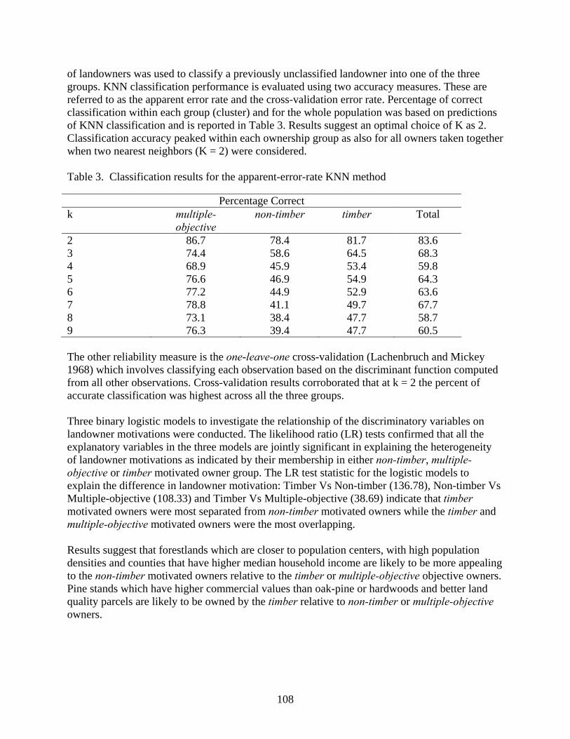
108

of landowners was used to classify a previously unclassified landowner into one of the three groups. KNN classification performance is evaluated using two accuracy measures. These are referred to as the apparent error rate and the cross-validation error rate. Percentage of correct classification within each group (cluster) and for the whole population was based on predictions of KNN classification and is reported in Table 3. Results suggest an optimal choice of K as 2. Classification accuracy peaked within each ownership group as also for all owners taken together when two nearest neighbors (K = 2) were considered.

Table 3. Classification results for the apparent-error-rate KNN method

Percentage Correct k multiple-

objective non-timber timber Total

2 86.7 78.4 81.7 83.6 3 74.4 58.6 64.5 68.3 4 68.9 45.9 53.4 59.8 5 76.6 46.9 54.9 64.3 6 77.2 44.9 52.9 63.6 7 78.8 41.1 49.7 67.7 8 73.1 38.4 47.7 58.7 9 76.3 39.4 47.7 60.5 The other reliability measure is the one-leave-one cross-validation (Lachenbruch and Mickey 1968) which involves classifying each observation based on the discriminant function computed from all other observations. Cross-validation results corroborated that at k = 2 the percent of accurate classification was highest across all the three groups. Three binary logistic models to investigate the relationship of the discriminatory variables on landowner motivations were conducted. The likelihood ratio (LR) tests confirmed that all the explanatory variables in the three models are jointly significant in explaining the heterogeneity of landowner motivations as indicated by their membership in either non-timber, multiple-objective or timber motivated owner group. The LR test statistic for the logistic models to explain the difference in landowner motivation: Timber Vs Non-timber (136.78), Non-timber Vs Multiple-objective (108.33) and Timber Vs Multiple-objective (38.69) indicate that timber motivated owners were most separated from non-timber motivated owners while the timber and multiple-objective motivated owners were the most overlapping. Results suggest that forestlands which are closer to population centers, with high population densities and counties that have higher median household income are likely to be more appealing to the non-timber motivated owners relative to the timber or multiple-objective objective owners. Pine stands which have higher commercial values than oak-pine or hardwoods and better land quality parcels are likely to be owned by the timber relative to non-timber or multiple-objective owners.

109

Discussion This study indicates that landowners can be accurately classified into heterogeneous attitudinal groups (multiple-objective, non-timber and timber) using predetermined demographic (from Census) and woodlot (from FIA) variables using the KNN technique. The accuracy rate of classification of landowner groups is fairly high (Table 3). We found that bio-physical (SLOPE, SITE, FT and AGE), socio-economic (INC and DIST) and demographic (PGI and PD) variables had a strong association with landowner group profiles. Given the increasing number of family forest owners and the increasing proportion of timberland they own and manage as an ownership class, this study can effectively help in estimating the different adjustment factors for diversely motivated landowner groups in order to more accurately project future timber supply. We also explore the factors associated with landowner motivations and find consistently that with increases in population pressure the likelihood of a forest owner to be motivated by non-timber consumption purposes relative to timber production increases. Results also show that better quality and level land is ideal for timber production and is likely to be owned by a timber producer with a profit motive. This also indicates that forests located closer to developed land (population centers) are likely to be subjected to a high opportunity cost for timber production and likely to be owned by individuals who value the aesthetic and recreational values of forests. On the other hand, rural areas with little development are more conducive to timber production and likely to be owned and managed by timber producers with the intent to produce timber for earning profit.

Literature Cited Alerich, C.L., Klevgard, L., Liff, C. and Miles, P.D. 2004. The Forest Inventory and Analysis

Database: Database Description and Users Guide Version 1.7. Fix, E. and Hodges, J. 1951. Discriminatory analysis, nonparametric discrimination: consistency

properties. Technical Report, Randolph Field, Texas: USAF School of Aviation Medicine. Johnson, R.A., and Wichern, D.W. 2002. Applied multivariate statistical data analysis. Prentice

Hall, 5th edition, Upper Saddle River, NJ 767pp. Klecka, W.R. 1988. Discriminant Analysis. Sage University Paper series on Quantitative

Applications in the Social Sciences, series no. 07-019. Beverly Hills and London: Sage Publications.

Lachenbruch, P.A., and Mickey, M.R. 1968. Estimation of Error Rates in Discriminant Analysis.

Technometrics. 10: 1-11. Majumdar, I., Teeter, L.D. and Butler, B.J. 2006. NIPFs in the Southeast: A diverse group with

diversified objectives. Presented at the Southern Forest Economics Workshop meeting 23-24 March 2006, Knoxville TN.

110

Wear, D. N. and J. G. Greis 2002. Southern Forest Resource Assessment: Technical Report. GTR-SRS-053. USDA Forest Service Southern Research Station. 635p.

111

Biofuel Production Impacts on the Management of Southern Pine Plantations in Mississippi∗

Zhimei Guo1, Donald L. Grebner2, Changyou Sun3, and Stephen C. Grado4

Abstract: This study evaluated and compared alternative forest management regimes of loblolly pine (Pinus taeda) plantations for producing both traditional timber commodities and biofuels. Land expectation values (LEV) and mean annual increments (MAI) of total biomass were applied as economic and biological criteria to determine the optimal management activities for different site indices and drainage classes in Mississippi. PTAEDA3.1 growth and yield model was used to predict the growth effects of different site preparations, initial planting density, fertilization, and thinning activity. Results indicated that on SI 50 to 60 lands, the average annual yields of stem residues were 0.76 to 1.14 tons per acre, or 30-45.1 gallons of ethanol. Wider planting spacings with a later thinning age and longer rotation length were financially optimal on lower quality lands. When maximizing MAI of total biomass, the intensive bedding combination became an optimal site treatment on poorly drained land. This site preparation practice, however, appeared unprofitable in terms of LEVs due to high operation costs. Results of sensitivity analysis indicated that the rise of relative biomass price to sawtimber will shorten the optimal thinning year and rotation age. Keywords: Biofuels, biomass availability, forest biomass, Mississippi, optimal management strategy, southern pine plantations Introduction

Recently, there has been an increased interest in biofuels and other forms of bioenergy by the general public in the United States because of a concern over energy prices, global climate changes, and energy security. Politically, it has the promising potential to revitalize rural America. Using forest biomass for biofuels not only reduces wildfire risk but also the pressure on agricultural land for biofuel production. Currently, the bio-technologies using woody biomass (i.e., fermentation, gasification, pyrolysis) have been in the development and demonstration stage. Specifically, pyrolysis technology uses small, modular, and transportable equipment that can be located near available feedstock sources. This can greatly lower

∗ Approved for publication as Journal Article No. FO 346 of the Forest and Wildlife Research Center, Mississippi State University. Financial and logistical support for this project was provided by the Mississippi State University Forest and Wildlife Research Center and USDA Wood Utilization Research Special Grants. 1 Graduate Research Assistant, Mississippi State University, Department of Forestry, PO Box 9681, Mississippi State, MS 39762, zg21@msstate.edu, (662)-325-8357 (v). 2 Associate Professor, Mississippi State University, Department of Forestry, PO Box 9681, Mississippi State, MS 39762, dgrebner@cfr.msstate.edu, (662)-325-0928 (v). 3 Assistant Professor, Mississippi State University, Department of Forestry, PO Box 9681, Mississippi State, MS 39762, csun@cfr.msstate.edu, (662)-325-7271 (v). 4 Professor, Mississippi State University, Department of Forestry, PO Box 9681, Mississippi State, MS 39762, sgrado@cfr.msstate.edu, (662)-325-2792 (v).

112

transportation costs and generates a value-added product. The emerging use of woody biomass will create a desirable alternative market for small diameter wood on forest lands in the Southern U.S. In Mississippi, approximately 20 million acres of forest land comprises 62% of the total land base and the forest products industry greatly contributes to state economy (Munn and Tilley 2005). Due to a declining demand for domestic wood pulp in global markets, forest management faces increasing challenges. Also, markets for thinning materials from young southern pine stands are limited because of the presence of high levels of juvenile wood. This condition may make first thinnings unprofitable, and consequently reduce the intensity by which timberlands are managed. Therefore, the utilization of forest biomass for biofuel production represents a real opportunity for forest management and rural economic development. Various studies examining biomass supply for bio-production have been performed in the United States, and have looked at resource assessment, potential supply and cost, and land management (Young et al. 1991; Cook and Beyea 2000; McNeil Technologies 2003). Some research explored the supply of short-rotation woody biomass or energy crops regionally (Downing and Graham 1996; Rosenqvist and Dawson 2005). Other studies assessed the generation, availability, and costs of different categories of biomass regionally or nationally such as agricultural residue, wood product residue, urban wood wastes, logging residues, and other forest biomass for bio-production (Howard 1981; Walsh et al. 2000; Kerstetter and Lyons 2001; McNeil Technologies 2003). McNeil Technologies (2003) looked at three counties in eastern Oregon and indicated that there is a need to modify existing forest and agricultural practices to make biomass available for bio-production regionally. Recent studies have also examined increasing productivity of forestry management and compared eco-economic benefits among different land management alternatives for biomass (Cook and Beyea 2000; Bjornstad and Skonhoft 2002; Mead 2005). It was found that biomass derived from the forest was significantly less expensive than an energy crop and there were also institutional and infrastructural obstacles to large-scale energy crop production. Based on the current wood market situation in Mississippi and the southern U.S., this study investigated the impact of biofuel production using small diameter wood on the management of loblolly pine (Pinus Taeda) plantations, which is widely distributed across Mississippi and the southern U.S., and the availability of forest biomass resulting from optimal management regimes on various sites within Mississippi. The specific study objectives were to: (1) evaluate and compare alternative forest management regimes and find economically and biologically optimal management strategies for forest landowners; (2) calculate available forest biomass for biofuel production resulting from economically optimal management regimes; and (3) explore how optimal forest management strategies and biomass availability are subject to changes in the relative price of biomass to sawtimber.

Methods To explore the impact of this emerging wood use on forest management, this study focused only on stem wood, whereas the other biomass from branches, twigs, leaves, and roots were beyond the scope of this research. In achieving the stated objectives, PTAEDA3.1 was used to predict

113

the yield data of the total stem and three wood classes: sawtimber, chip-n-saw, and pulpwood. The weight of stem residue1 was then calculated by subtracting the weight of three wood commodities from total stem biomass. Using this yield information, land expectation value (LEV) and mean annual increment (MAI) of total stem biomass were calculated to evaluate and compare alternative management regimes. A sensitivity analysis was then conducted to show how optimal forest management strategies and biomass availability were subject to changes in the relative price of biomass to sawtimber. Economic and Biological Evaluation This study assumed that stumpage prices were stable and no inflation would occur. LEVs were calculated for each management scenario using a before-tax, real annual discount rate of 5%, which is similar to a forest landowner’s real rate of return. Revenues from stem residues from thinning and harvesting were included in the Faustmann model for determining economic returns. The management regime which maximized the LEV was considered optimal for each specific site. The optimal management regimes which culminate the MAI of total stem biomass for biofuel production was also determined for each site to allow for more options in the decision making process. MAIs were calculated by dividing the green weight of the total stem by rotation age. This biological model helped find the maximum sustainable annual output of total stem biomass for biofuel production on each site. LEVs of these optimal regimes were calculated using exclusively the biomass price (i.e., stem residue price), since whole stands were managed for biofuel production.

Available Biomass and Biofuel Production Estimation Average annual yields of stem residues and pulpwood resulting from optimal management regimes were calculated by dividing those outputs from thinning and harvesting by rotation age. This information can serve as a basis for estimating annual biofuel production. This study estimated the annual ethanol production on a per acre basis. First, green tons of stem biomass were converted to dry weight according to the moisture content of loblolly pine sapwood (106 grams of water per 100 gram of dry wood) (FPL, 1999). That is, a green ton of stem biomass can be converted to 0.485 ton of dry wood. The theoretical ethanol conversion rate for feedstock from forest thinnings is 81.5 gallons per dry ton, which was then used to calculate the potential ethanol production per acre of loblolly pine plantation (DOE, 2006). Management Scenarios Site indices of 50 and 60 (base age 25) combined with two drainage classes (i.e., poor, well) represent the potential sites that exist across loblolly pine plantations in Mississippi. This site index range will help examine how site productivity influences economic returns, available biomass, and optimal management strategies. The site preparation practices for well-drained land considered in this study included a combination of chop and burn, herbaceous weed control, 1 Stem residue in this study refers to small diameter trees with a DBH less than 6 inches and topwood from three wood commodities: sawtimber, chip-n-saw, and pulpwood.

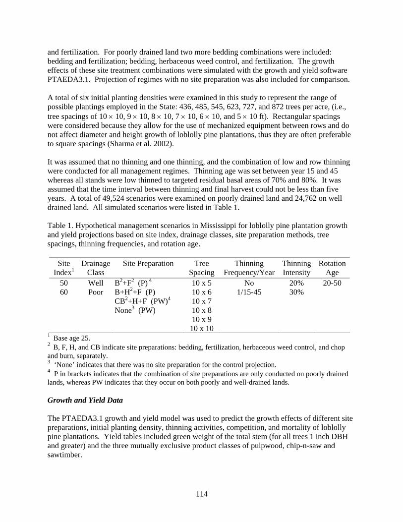
114

and fertilization. For poorly drained land two more bedding combinations were included: bedding and fertilization; bedding, herbaceous weed control, and fertilization. The growth effects of these site treatment combinations were simulated with the growth and yield software PTAEDA3.1. Projection of regimes with no site preparation was also included for comparison. A total of six initial planting densities were examined in this study to represent the range of possible plantings employed in the State: 436, 485, 545, 623, 727, and 872 trees per acre, (i.e., tree spacings of 10 × 10, 9 × 10, 8 × 10, 7 × 10, 6 × 10, and 5 × 10 ft). Rectangular spacings were considered because they allow for the use of mechanized equipment between rows and do not affect diameter and height growth of loblolly pine plantations, thus they are often preferable to square spacings (Sharma et al. 2002). It was assumed that no thinning and one thinning, and the combination of low and row thinning were conducted for all management regimes. Thinning age was set between year 15 and 45 whereas all stands were low thinned to targeted residual basal areas of 70% and 80%. It was assumed that the time interval between thinning and final harvest could not be less than five years. A total of 49,524 scenarios were examined on poorly drained land and 24,762 on well drained land. All simulated scenarios were listed in Table 1.

Table 1. Hypothetical management scenarios in Mississippi for loblolly pine plantation growth and yield projections based on site index, drainage classes, site preparation methods, tree spacings, thinning frequencies, and rotation age.

Site Index1

Drainage Class

Site Preparation

Tree Spacing

Thinning Frequency/Year

Thinning Intensity

Rotation Age

50 60

Well Poor

B2+F2 (P) 4 B+H2+F (P) CB2+H+F (PW)4 None3 (PW)

10 x 5 10 x 6 10 x 7 10 x 8 10 x 9 10 x 10

No 1/15-45

20% 30%

20-50

1 Base age 25. 2 B, F, H, and CB indicate site preparations: bedding, fertilization, herbaceous weed control, and chop and burn, separately. 3 ‘None’ indicates that there was no site preparation for the control projection. 4 P in brackets indicates that the combination of site preparations are only conducted on poorly drained lands, whereas PW indicates that they occur on both poorly and well-drained lands. Growth and Yield Data The PTAEDA3.1 growth and yield model was used to predict the growth effects of different site preparations, initial planting density, thinning activities, competition, and mortality of loblolly pine plantations. Yield tables included green weight of the total stem (for all trees 1 inch DBH and greater) and the three mutually exclusive product classes of pulpwood, chip-n-saw and sawtimber.

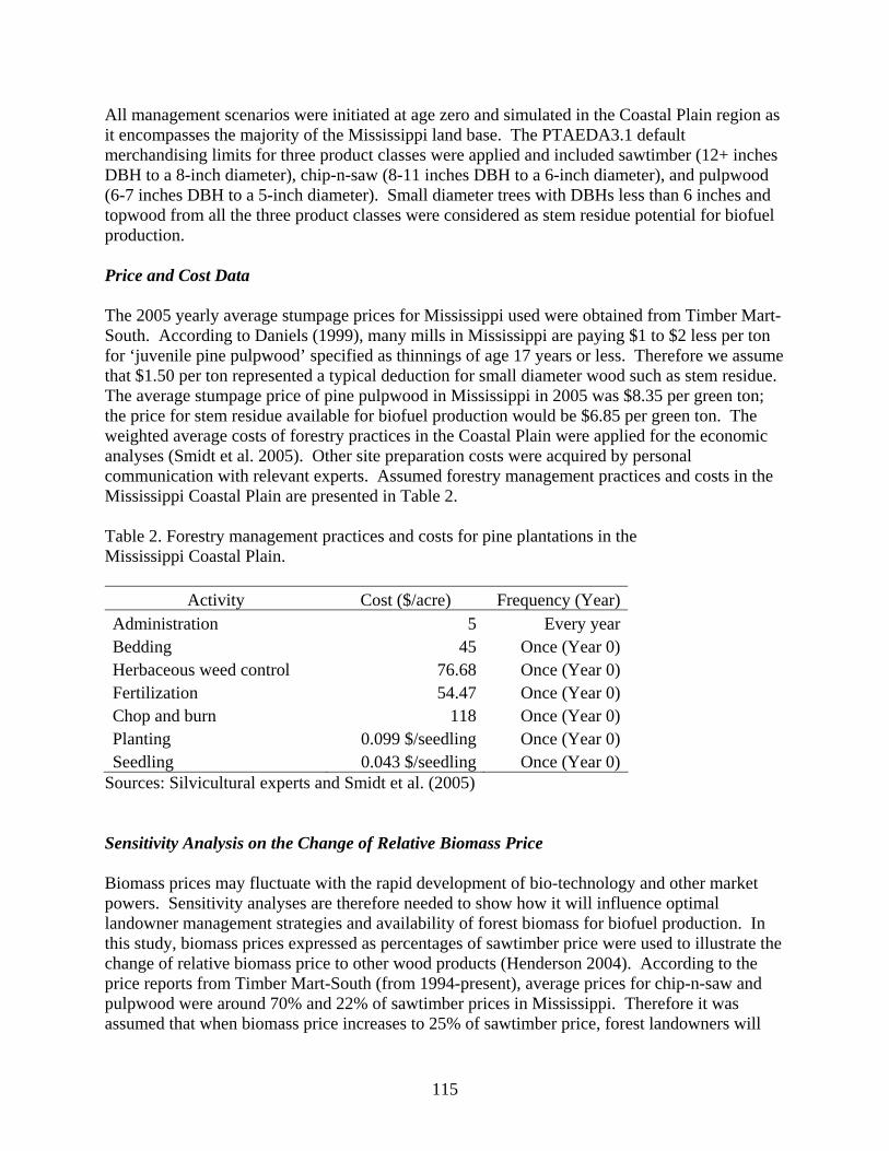
115

All management scenarios were initiated at age zero and simulated in the Coastal Plain region as it encompasses the majority of the Mississippi land base. The PTAEDA3.1 default merchandising limits for three product classes were applied and included sawtimber (12+ inches DBH to a 8-inch diameter), chip-n-saw (8-11 inches DBH to a 6-inch diameter), and pulpwood (6-7 inches DBH to a 5-inch diameter). Small diameter trees with DBHs less than 6 inches and topwood from all the three product classes were considered as stem residue potential for biofuel production.

Price and Cost Data The 2005 yearly average stumpage prices for Mississippi used were obtained from Timber Mart-South. According to Daniels (1999), many mills in Mississippi are paying $1 to $2 less per ton for ‘juvenile pine pulpwood’ specified as thinnings of age 17 years or less. Therefore we assume that $1.50 per ton represented a typical deduction for small diameter wood such as stem residue. The average stumpage price of pine pulpwood in Mississippi in 2005 was $8.35 per green ton; the price for stem residue available for biofuel production would be $6.85 per green ton. The weighted average costs of forestry practices in the Coastal Plain were applied for the economic analyses (Smidt et al. 2005). Other site preparation costs were acquired by personal communication with relevant experts. Assumed forestry management practices and costs in the Mississippi Coastal Plain are presented in Table 2.

Table 2. Forestry management practices and costs for pine plantations in the Mississippi Coastal Plain.

Activity Cost ($/acre) Frequency (Year)Administration 5 Every yearBedding 45 Once (Year 0)Herbaceous weed control 76.68 Once (Year 0)Fertilization 54.47 Once (Year 0)Chop and burn 118 Once (Year 0)Planting 0.099 $/seedling Once (Year 0)Seedling 0.043 $/seedling Once (Year 0)

Sources: Silvicultural experts and Smidt et al. (2005)

Sensitivity Analysis on the Change of Relative Biomass Price Biomass prices may fluctuate with the rapid development of bio-technology and other market powers. Sensitivity analyses are therefore needed to show how it will influence optimal landowner management strategies and availability of forest biomass for biofuel production. In this study, biomass prices expressed as percentages of sawtimber price were used to illustrate the change of relative biomass price to other wood products (Henderson 2004). According to the price reports from Timber Mart-South (from 1994-present), average prices for chip-n-saw and pulpwood were around 70% and 22% of sawtimber prices in Mississippi. Therefore it was assumed that when biomass price increases to 25% of sawtimber price, forest landowners will

116

sell pulpwood for biofuel production. When biomass price increases to 70% or 100% of sawtimber prices, even chip-n-saw or sawtimber can be considered for biofuel production. When biomass price falls at or below 10% of sawtimber prices, only stem residues are available for biofuel production. Results Optimal Management Regimes Maximizing LEV Land expectation values for all management scenarios were calculated. The combination of initial planting density, site preparation practice, thinning, and rotation age which resulted in the highest LEV was identified as financially optimal. The optimal management regime and its LEV at a 5% real discount rate for each combination of site index and drainage class were listed in Table 3. LEVs ranged from $579 to 797 from site index 50 to 60. The regimes with site preparation treatments were not cost effective in comparison to scenarios with no site preparation for all the sites. The optimal initial planting density varied in response to differences in site productivity. Wider spacings with longer thinning ages appeared optimal on lower productivity land, whereas closer spacings with earlier thinning ages appeared optimal on higher productivity sites. When site index increases, the optimal rotation length decreases. The optimal thinning intensity results showed no relevance to site quality; however, it does vary with the interaction of all factors which include site index, initial planting density, thinning age, and rotation length.

Table 3. Financially optimal management regimes of loblolly pine plantation in Mississippi and land expectation values (LEV) by site index and drainage class at 5% real discount rate.

Optimal Regimes Site Index1

Drainage Class Site

Preparation Density

(tree/acre) Thinning

(year) Rotation Age

(year)

LEV $/acre

Poor none 436 21 (20%)2 35 579 50

Well none 436 18 (30%) 34 581 Poor none 545 16 (30%) 29 759

60 Well none 545 17 (20%) 28 797

1 Base age 25. 2 Percentage numbers in brackets are the percentage of basal area removed during low thinning.

Average annual yields of stem residues potentially available for biofuel production from financially optimal management regimes at a 5% discount rate for different site combination are presented on a per acre basis (Table 4). According to the current market condition for small diameter wood, it was possible to include pulpwood for biofuel production. Thus, the sum of annual yields of stem residues and pulpwood was also listed. Ethanol production per acre of loblolly pine plantations were calculated and presented in brackets. They ranged from 58.5 to 80.2 gal/ac/yr from site index 50 to 60. Results indicated that higher site quality yields more annual stem residue and pulpwood; therefore, more ethanol can be produced.

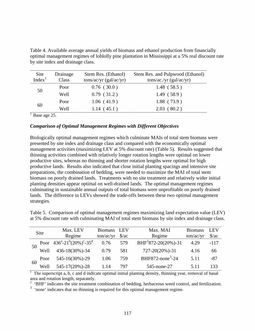
117

Table 4. Available average annual yields of biomass and ethanol production from financially optimal management regimes of loblolly pine plantation in Mississippi at a 5% real discount rate by site index and drainage class.

Site Index1

Drainage Class

Stem Res. (Ethanol) tons/ac/yr (gal/ac/yr)

Stem Res. and Pulpwood (Ethanol) tons/ac./yr (gal/ac/yr)

Poor 0.76 ( 30.0 ) 1.48 ( 58.5 ) 50

Well 0.79 ( 31.2 ) 1.49 ( 58.9 ) Poor 1.06 ( 41.9 ) 1.88 ( 73.9 )

60 Well 1.14 ( 45.1 ) 2.03 ( 80.2 )

1 Base age 25. Comparison of Optimal Management Regimes with Different Objectives Biologically optimal management regimes which culminate MAIs of total stem biomass were presented by site index and drainage class and compared with the economically optimal management activities (maximizing LEV at 5% discount rate) (Table 5). Results suggested that thinning activities combined with relatively longer rotation lengths were optimal on lower productive sites, whereas no thinning and shorter rotation lengths were optimal for high productive lands. Results also indicated that close initial planting spacings and intensive site preparations, the combination of bedding, were needed to maximize the MAI of total stem biomass on poorly drained lands. Treatments with no site treatment and relatively wider initial planting densities appear optimal on well-drained lands. The optimal management regimes culminating in sustainable annual outputs of total biomass were unprofitable on poorly drained lands. The difference in LEVs showed the trade-offs between these two optimal management strategies.

Table 5. Comparison of optimal management regimes maximizing land expectation value (LEV) at 5% discount rate with culminating MAI of total stem biomass by site index and drainage class.

Site Max. LEV Regime

Biomass ton/ac/yr

LEV $/ac

Max. MAI Regime

Biomass ton/ac/yr

LEV $/ac

Poor 436a-21b(20%)c-35d 0.76 579 BHF2872-20(20%)-31 4.29 -117 50

Well 436-18(30%)-34 0.79 581 727-20(20%)-31 4.16 66 Poor 545-16(30%)-29 1.06 759 BHF872-none3-24 5.11 -87

60 Well 545-17(20%)-28 1.14 797 545-none-27 5.11 133

1 The superscript a, b, c and d indicate optimal initial planting density, thinning year, removal of basal area and rotation length, separately. 2 ‘BHF’ indicates the site treatment combination of bedding, herbaceous weed control, and fertilization. 3 ‘none’ indicates that no thinning is required for this optimal management regime.

118

Sensitivity Analysis on the Change of Relative Biomass Price The sensitivity analysis results for site index 60, well-drained lands represented the general trend that appeared on various sites considered in this study. It indicated that when relative biomass price changed from 10 to 100% of the sawtimber price, the initial planting density increased from 545 to 727 trees per acre. The changing trends of rotation age, optimal thinning activities, and available biomass were presented in Figure 1. It showed that when relative biomass price increases, optimal thinning year and rotation age decreased; optimal thinning intensity appeared irrelevant to biomass price change, whereas the available mean annual stem biomass increased because pulpwood, chip-n-saw and even sawtimber can be included for biofuel production.

0

5

10

15

20

25

30

10% 25% 70% 100%

Relative biomass price to sawtimber

Rotation age

Thinning year

Removal (%)

Avail. Biomass(tons/ac/yr)

Figure 1. Comparison of optimal thinning activities, rotation age, and mean annual yield of forest biomass available for biofuel production from loblolly pine plantation on site index 60, well-drained lands when relative biomass price to sawtimber price changes. Discussion Both LEVs and sustainable annual yields of total biomass were maximized using proper management activities, such as site preparation, initial planting density, thinning age, and rotation length. Combinations of site preparation treatments considered were not cost effective in comparison to no site preparation for all sites, (i.e., cost inputs were greater than gains from growth). Possible reasons may be: 1) the stand growth predicted by the PTAEDA simulator was too conservative in terms of fertilization effects; 2) the economic evaluation is overly sensitive to higher costs of intensive site preparations. Wider spacings with a later thinning age and longer rotation length were financially optimal on lower quality lands. The optimal thinning intensity showed an irrelevance to site quality only but varied with the interaction of all factors: site index, initial planting density, thinning age, and rotation length. When maximizing MAI of total biomass, the intensive bedding combination became an optimal site treatment on poorly drained land. This site preparation practice, however, appeared unprofitable in terms of LEVs due to high operation costs.

119

Site index has a substantial effect on LEV, available stem residue biomass, and the optimal management strategies whether to maximize LEV or culminate MAI of total biomass. When site index increases, the average annual stem residue biomass available for biofuel production increases. The other effects in terms of LEVs, financially optimal thinning age, and rotation length were consistent with results of previous studies. Results of this sensitivity analysis indicated that the rise of relative biomass price to sawtimber will shorten the optimal thinning year and rotation age, which was also reasonable because management strategies will gradually evolve to maximize total biomass. Conclusions The emerging use of wood has the potential to provide new opportunities and markets for forest landowners in Mississippi and the Southern U.S. This study showed that on SI 50 to 60 lands, the average annual yields of stem residues were 0.76 to 1.14 tons per acre, or 30-45.1 gallons of ethanol. Culminating sustainable annual outputs of total stem biomass were unprofitable on poorly drained lands due to high site preparation costs at currently low biomass prices. This study extended previous research by examining the influence of various site preparation techniques on optimal management strategies. Examining changes in relative biomass prices to sawtimber prices was useful in evaluating the availability of biomass for bio-production. The results can be beneficial to both the bio-production industry and private forest landowners in the southern United States, especially in Mississippi. Future research should include additional site preparation practices for economic evaluations and comparisons. Literature Cited Bjornstad, E. and A. Skonhoft. 2002. Wood fuel or carbon sink? Aspects of forestry in the

climate question. Environmental and Resource Economics 23(2): 447-465.

Cook, J. and J. Beyea. 2000. Bioenergy in the United States: progress and possibilities. Biomass and Bioenergy 18(6): 441-455.

Daniels, R.A. 1999. Mississippi timber price report - March/April 1999. Mississippi State University Extension Service, Mississippi Agricultural and Forestry Experiment Station. 4 p.

Downing, M. and R.L. Graham. 1996. The potential supply and cost of biomass from energy crops in the Tennessee Valley Authority region. Biomass and Bioenergy 11(4): 283-303.

Forest Products Laboratory. 1999. Wood Handbook – Wood as an engineering material. U.S. Department of Agriculture, Forest Service, Forest Products Laboratory, USA. Gen. Tech. Rep. FPL-GTR-113, Madison, WI, 463 p.

Henderson, J.E. 2004. The impact of relative product prices on the optimal management regime

for loblolly pine plantations. M.Sc. thesis, Mississippi State University. Mississippi State. 194 p.

120

Howard, J.O. 1981. Ratios for estimating logging residue in the Pacific Northwest. Pacific Northwest Forest and Range Experiment Station, Portland, Oregon, USDA Forest Service. 26 p.

Kerstetter, J.D. and J.K. Lyons. 2001. Logging and agricultural residue supply curves for the Pacific Northwest. Washington State University Energy Program. 45 p.

McNeil Technologies, Inc. 2003. Biomass resource assessment and utilization options for three counties in Eastern Oregon. Lakewood, Colorado. 177 p.

Mead, D. J. 2005. Opportunities for improving plantation productivity. How much? How quickly? How realistic? Biomass and Bioenergy 28(4): 249-266.

Munn, I.A. and B.K. Tilley. 2005. Forestry in Mississippi - The impact of the forest products industry on the Mississippi economy: An input-output analysis. Mississippi State University: 27 p.

Rosenqvist, H. and M. Dawson. 2005. Economics of willow growing in Northern Ireland. Biomass and Bioenergy 28(1): 7-14.

Smidt, M., M.R. Dubois and B.d.S. Folegatti. 2005. Costs and cost trends for forestry practices in the South. Forest Landowner 64(2): 25-31.

U.S. Department of Energy. 2006. Energy efficiency and renewable energy biomass program. http://www1.eere.energy.gov/biomass/printable_versions/ethanol_yield_calculator.html

Walsh, M.E., R.L. Perlack, A. Turhollow, D.d.l.T. Ugarte, D.A. Becker, R.L. Graham, S.E.

Slinsky and D.E. Ray. 2000. Biomass feedstock availability in the United States: 1999 state level analysis. Biomass Feedstock Information Network. Available from http://bioenergy.ornl.gov/resourcedata/index.html.

Young, T.M., D.M. Ostermeier, J.D. Thomas and R.T. Brooks. 1991. The economic availability of woody biomass for the southeastern United States. Bioresource Technology 37(1): 7-15.

121

Woody Biomass Feedstock Supplies and Management for Bioenergy in Southwestern Mississippi*

Gustavo Perez-Verdin1, Donald Grebner2, Changyou Sun2, Ian Munn2, Emily Schultz2, and Thomas Matney2

Abstract: Mississippi’s forests cover approximately 20 million acres distributed in hardwood, softwood, or combination of both forest types. This timberland acreage represents a source of woody biomass for potential bioenergy consumption derived from four processes: (1) residues associated with the harvesting and managing of conventional forest products such as sawlogs, pulpwood, and veneer logs, in which material is often left on-site or piled and burned at an additional cost; (2) biomass generated from thinning to improve forest health and reduce fire hazard risks; (3) residues from mills; and (4) urban waste. Although there are many studies of woody biomass use for bioenergy consumption, few have analyzed the economic feasibility of utilizing woody biomass as a feedstock to produce ethanol in Mississippi. In this study, using forest inventory data from the Mississippi Institute for Forestry Inventory, we estimate woody biomass supplies by county, evaluate their availability for potential use in bioethanol facilities, and analyze major production costs. Results show that more than 975,000 dry tons are available for use as a potential feedstock to produce ethanol. Logging residues and small-diameter trees make up the majority of these stocks (89%) with much less from mills and urban waste (11%). However, small-diameter biomass was the most expensive feedstock due to the high costs of delivery which included the price paid to the owner for the right to harvest. In general, transportation costs account between 50 and 60 percent of total production costs. Keywords: Ethanol, forestry residues, production costs, supply curves, thinning woody biomass Introduction Bioenergy can be converted from a wide variety of agricultural and forestry resources, including corn, sugarcane, wood, industrial processing residues, and municipal solid and urban wood waste (Perlack and others 2005). Cellulosic ethanol, one of several bioenergy outputs, is fuel ethanol made from cellulose, hemicellulose, and lignin. Cellulose is the inedible fiber that forms the stems and branches of plants and represents the main component of plant cell walls (Crooks 2006). Since cellulose is the most common organic compound on earth, it is one of the most promising feedstocks for conversion into liquid transportation fuels (Coleman and Stanturf

* Approved as manuscript FO345, Forest and Wildlife Research Center, Mississippi State University. We thank the Mississippi Forestry Commission and the Mississippi Institute for Forest Inventory for allowing us to use the forest inventory data. Drs. Anwar Hussain and Deborah Gaddis provided valuable comments in an early manuscript of this research. We thank John Cason for his assistance in gathering information. This study is being financially supported by the Sustainable Energy Research Center at Mississippi State University. 1 Postdoc Research Associate, Department of Forestry, Mississippi State University, Box 9681, Mississippi State, MS 39762, gperez@cfr.msstate.edu, (662) 325-6822 (v). 2 Associate Professor, Assistant Professor, Professor, Associate Professor, and Professor, respectively, Mississippi State University, Box 9681, Mississippi State, MS 39762.

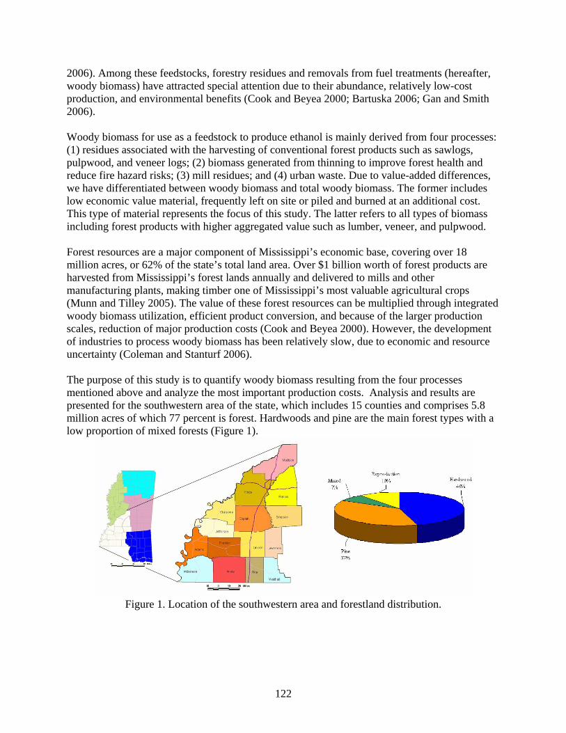
122

2006). Among these feedstocks, forestry residues and removals from fuel treatments (hereafter, woody biomass) have attracted special attention due to their abundance, relatively low-cost production, and environmental benefits (Cook and Beyea 2000; Bartuska 2006; Gan and Smith 2006). Woody biomass for use as a feedstock to produce ethanol is mainly derived from four processes: (1) residues associated with the harvesting of conventional forest products such as sawlogs, pulpwood, and veneer logs; (2) biomass generated from thinning to improve forest health and reduce fire hazard risks; (3) mill residues; and (4) urban waste. Due to value-added differences, we have differentiated between woody biomass and total woody biomass. The former includes low economic value material, frequently left on site or piled and burned at an additional cost. This type of material represents the focus of this study. The latter refers to all types of biomass including forest products with higher aggregated value such as lumber, veneer, and pulpwood. Forest resources are a major component of Mississippi’s economic base, covering over 18 million acres, or 62% of the state’s total land area. Over $1 billion worth of forest products are harvested from Mississippi’s forest lands annually and delivered to mills and other manufacturing plants, making timber one of Mississippi’s most valuable agricultural crops (Munn and Tilley 2005). The value of these forest resources can be multiplied through integrated woody biomass utilization, efficient product conversion, and because of the larger production scales, reduction of major production costs (Cook and Beyea 2000). However, the development of industries to process woody biomass has been relatively slow, due to economic and resource uncertainty (Coleman and Stanturf 2006). The purpose of this study is to quantify woody biomass resulting from the four processes mentioned above and analyze the most important production costs. Analysis and results are presented for the southwestern area of the state, which includes 15 counties and comprises 5.8 million acres of which 77 percent is forest. Hardwoods and pine are the main forest types with a low proportion of mixed forests (Figure 1).

Figure 1. Location of the southwestern area and forestland distribution.

123

Methods Data come from a recent forest inventory, timber production reports, and state surveys. The Mississippi Institute for Forest Inventory (MIFI) was created in 2002 to inventory the forest resources of the state. The inventory began in 2004 and currently the southwestern and southeastern portions of the state have been completed. The remainder of the forest inventory is expected to be completed by mid 2008. To gain experience and evaluate the consistency of the information for ethanol production, we are presenting results for the southwestern area as a preamble for a comprehensive study of all five regions. Data processing and reporting are done through a computer software, called the MIFI Dynamic Inventory Reporter [http://www.mifi.ms.gov/mission.htm], which captures and report both current and historical (US Forest Service) forest inventory information. The current forest inventory integrates a satellite-based remote sensing and stratified sampling design that produces near real-time inventory of the status of forest resources. Through a combination of band analysis and mathematical modeling, primary classifications of water, non-forest, pine, hardwoods, and mixed pine-hardwood classes are obtained from remote sensing. Ground-based measurements include four types of plots: (1) a one-fifth acre fixed radius plot located randomly within forest cover classes on which conventional products (saw timber, pole) along with stand dynamics attributes are measured; (2) a one-tenth acre plot on which all trees oriented for the pulp industry are recorded; (3) a one-twentieth acre plot for trees from 1 to 4.5 inches in diameter at breast height; and (4) a one-hundredth acre regeneration plot. From this inventory and timber production reports (Howell and others 2005), we calculated total inventories, growth, and removals. Total inventories include existing biomass from all types of species, natural and planted stands, conventional products, cull trees, and small diameter trees. Growth rate is the percent of biomass growing annually and is calculated from MIFI stand table projections. Removals refer to the amount of timber produced in any year and include conventional products such as sawlogs, pulpwood, and veneer logs. The availability of logging residues was obtained by estimating the proportion of branches to stem biomass. It was assumed that leaves are left on site for soil nutrient compensation (Sanchez and Eaton 2001). The branch-to-stem ratio was then multiplied by the amount of timber produced in 2002 based on Howell and others (2005). Small-diameter biomass was calculated by applying a rate of thinning of 60 percent over total biomass and a recovery rate of 80 percent (Harrington 2002; Perlack and others 2005) for all trees less than 8 inches in diameter at breast height. The harvest frequency was set at 30 years (Perlack and others 2005). Mill and urban waste were processed from USDA Forest Service Forest Inventory Analysis (FIA) data, state surveys (Garrard and Leightley 2005), and the Mississippi Department of Environmental Quality (information available at http://www.deq.state.ms.us/MDEQ.nsf/page/SW_Home?OpenDocument). Production costs include cutting, skidding, loading, and transporting woody biomass to the processing plant as well as payment to the owner for the right to harvest1. These costs can be divided in three types: harvest (cutting, skidding, and loading), transportation, and stumpage

1 Other plant processing costs such as equipment, installation, engineering, financing, labor, and marketing were not included. The scope of this project is to address only costs associated with processing, managing, and transporting woody biomass feedstocks to the converting facilities.

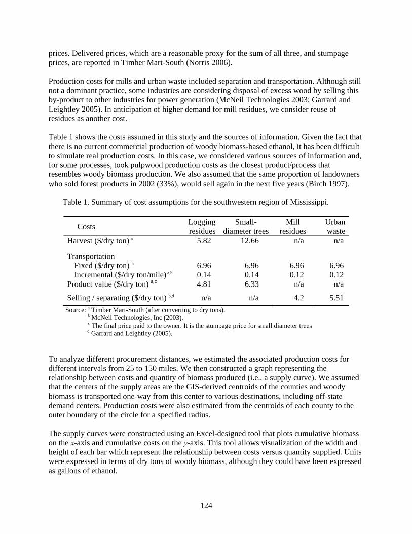
124

prices. Delivered prices, which are a reasonable proxy for the sum of all three, and stumpage prices, are reported in Timber Mart-South (Norris 2006). Production costs for mills and urban waste included separation and transportation. Although still not a dominant practice, some industries are considering disposal of excess wood by selling this by-product to other industries for power generation (McNeil Technologies 2003; Garrard and Leightley 2005). In anticipation of higher demand for mill residues, we consider reuse of residues as another cost. Table 1 shows the costs assumed in this study and the sources of information. Given the fact that there is no current commercial production of woody biomass-based ethanol, it has been difficult to simulate real production costs. In this case, we considered various sources of information and, for some processes, took pulpwood production costs as the closest product/process that resembles woody biomass production. We also assumed that the same proportion of landowners who sold forest products in 2002 (33%), would sell again in the next five years (Birch 1997). Table 1. Summary of cost assumptions for the southwestern region of Mississippi.

Costs Logging residues

Small-diameter trees

Mill residues

Urban waste

Harvest ($/dry ton) a 5.82 12.66 n/a n/a

Transportation Fixed ($/dry ton) b

Incremental ($/dry ton/mile) a,b

6.96 0.14

6.96 0.14

6.96 0.12

6.96 0.12

Product value ($/dry ton) a,c 4.81 6.33 n/a n/a

Selling / separating ($/dry ton) b,d n/a n/a 4.2 5.51 Source: a Timber Mart-South (after converting to dry tons). b McNeil Technologies, Inc (2003).

c The final price paid to the owner. It is the stumpage price for small diameter trees d Garrard and Leightley (2005).

To analyze different procurement distances, we estimated the associated production costs for different intervals from 25 to 150 miles. We then constructed a graph representing the relationship between costs and quantity of biomass produced (i.e., a supply curve). We assumed that the centers of the supply areas are the GIS-derived centroids of the counties and woody biomass is transported one-way from this center to various destinations, including off-state demand centers. Production costs were also estimated from the centroids of each county to the outer boundary of the circle for a specified radius. The supply curves were constructed using an Excel-designed tool that plots cumulative biomass on the x-axis and cumulative costs on the y-axis. This tool allows visualization of the width and height of each bar which represent the relationship between costs versus quantity supplied. Units were expressed in terms of dry tons of woody biomass, although they could have been expressed as gallons of ethanol.

125

A sensitivity analysis to assess the variations in production costs was performed by reducing the stumpage price of logging residues. Since logging residues are generated during normal harvest operations, one could assume that they do not have value and their final product value should be removed from total operation costs. Thus, we considered various product values including no payment to the landowner. A second variation of the sensitivity analysis was the assignment of different transportation costs and distances. Results Adjusting data for 20021, the year of timber production data used in this study (Howell and others 2005), there are 134.4 million dry tons of standing forest inventories in the 15-county southwestern region of Mississippi. The heaviest concentrations of timber resources are found in Wilkinson, Copiah, Hinds, Amite, and Rankin (Figure 2). The annual growth for all counties and species is 12.6 million dry tons, which represents 9.3 percent of inventories. Annual removals total 5 million dry tons (year 2002), which represents 3.7 and 39.6 percent of inventories and forest growth, respectively.

-

100

200

300

400

500

600

700

Adams

Amite

ClaiborneCopiahFranklinHindsJeffersonLawrenceLincolnM

adisonPike

RankinSim

psonW

althallW

ilkinsonM

illio

n ft3 Inventory Anual growth Removals

Figure 2. Inventories, annual growth, and removals for the southwestern area of

Mississippi (2002). Woody biomass availability The annual woody biomass availability for the 15-county area is 975,000 dry tons. Of this amount, 74 percent are logging residues, 15 percent are small-diameter trees, 5 percent are urban waste, and 6 percent are produced from mill residues. Logging residues and small-diameter trees combined yield between 4.5 to 8.5 dry tons/acre/year (in this case, yield is dry tons divided by forest area), with an average of 6.8 dry tons/acre/year. The ratio of timber production to logging residues is 6.7, which means that 6.7 tons of conventional timber production generates one ton of

1 Data were adjusted by discounting the accumulated growth with respect to 2007. Growth rates for each county were obtained from the MIFI reporter.

126

logging residues. Assuming 80 gallons of ethanol per dry ton of woody biomass (DOE 2007, http://www1.eere.energy.gov/biomass/ethanol_yield_calculator.html) and a manufacturing plant energy efficiency of 35 percent (Hamelinck and others 2005; Gan and Smith 2006) the total production of ethanol can reach up to 27 million gallons per year or, in energy units, 2.3 millions of MMBtu, which is equivalent to the 0.0002 percent of the total US energy consumed in 2005 (EIA 2005). The southwest Mississippi counties with the greatest ethanol potential are Amite, Copiah, and Rankin (Figure 3).

Figure 3. Biomass availability for the southwestern MIFI inventory region of Mississippi.

We conducted a temporal analysis of small diameter trees availability using stand table projections of gross growth from the MIFI Dynamic Inventory Reporter. Since logging residues basically depend on the amount of timber harvested, they were not included in these data projections. Instead, we used a percent change of timber harvested from 2000 to 2005 and applied the 2002 timber production to logging residues ratio to estimate the trends for the following years (Gan and Smith 2006). The percent change rw was calculated as follows:

1

1 2

1

1 1t

w

A Ar

A⎛ ⎞−

= − −⎜ ⎟⎜ ⎟⎝ ⎠

where w is species group (pine or hardwood), A1 is the timber production at time 1, A2 is the timber production at time 2, and t is the number of years for the period of analysis. Based on timber severance data (Mississippi State Tax Commission, http://msucares.com/forestry/ economics/reports/index.html), the percent changes for this period were: pine -0.013, hardwoods -0.094, for a combined rate of -0.042. We assumed no substantial variations in the amount of mill residues and urban waste. The results of the projections for the next five years are shown in Figure 4.

127

0

100

200

300

400

500

600

700

800

900

2007 2008 2009 2010 2011

T

Thou

sand

dry

tons Mills residues Urban waste Small-diameter trees Logging residues

Figure 4. Annual woody biomass supplies for the southwestern MIFI inventory region of Mississippi.

Accordingly, Figure 4 shows a slight decrease in the availability of logging residues driven by a reduction in harvests of pulpwood, mostly from hardwoods. In 2000, production of pulpwood from hardwoods was 398 million ft3 whereas in 2005 production was only 240 million ft3 (Mississippi State Tax Commission, information available at http://msucares.com/forestry/ economics/reports/index.html). In contrast, small-diameter biomass shows a significant increase due to a higher growth rate and reduced harvesting. Production costs The resulting supply curves suggest that woody biomass from small-diameter trees are more costly than the other sources of biomass. In fact, mill residues and urban waste from distances up to 150 miles can compete with closer, more expensive biomass. However, mill residues and urban waste make up a small percentage of total supply. Reducing the product value of logging residues (while keeping constant all other costs) produced no significant results until it is equal or less than one. For any product value between $1 and 14, logging residues are the second most expensive feedstock, only behind small-diameter trees. When the product value is equal or less than one, logging residues becomes the second less expensive, only behind mill residues. For all woody biomass types, transportation costs accounted for the majority of production costs (50–60%). Based on the weighted average for all woody biomass, total production costs per dry ton are: $25.1 for a 50-mile radius, $27.6 for 100-mile radius, and $33.2 for 150-mile radius. Individual costs by woody biomass source are shown in Figure 5.

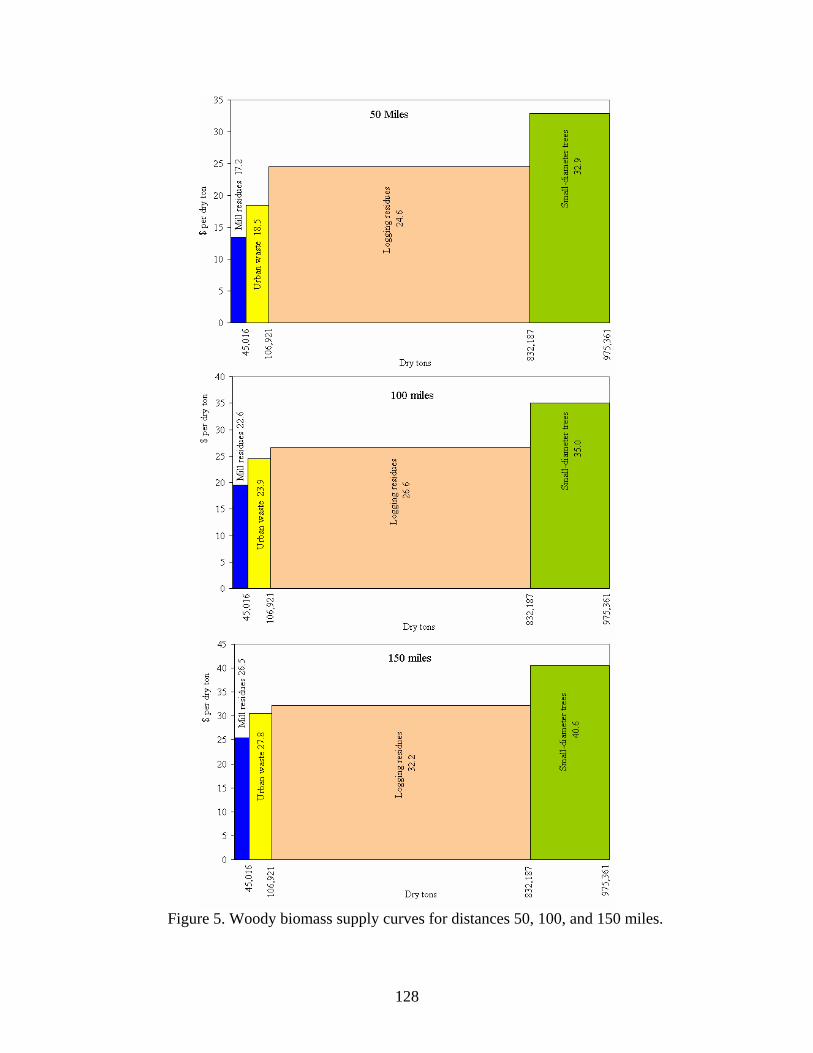
128

Figure 5. Woody biomass supply curves for distances 50, 100, and 150 miles.

129

Conclusions This research was conducted to estimate woody biomass availability from logging residues, small-diameter trees, mills residues, and urban waste sources as a feedstock to produce ethanol in the 15-county southwestern MIFI inventory region in Mississippi. We used MIFI’s recent forest inventory and Dynamic Inventory Reporter to provide accurate information on the distribution and quantity of timber resources. Other sources of information included state reports on woody biomass and USFS FIA data. Results showed that the annual woody biomass available in the Mississippi’s southwestern 15-county area is 975 thousands dry tons (excluding conventional forest products such as sawlogs and veneer logs which have higher aggregated value). These stocks can produce up to 27 millions gallons of ethanol per year. The counties with the highest biomass potential are Amite, Copiah, and Rankin. Logging residues and overstocked stands (small-diameter trees) make up the majority of woody biomass supplies (89%) whereas the non-used portion of mill residues and urban waste contributed to 5 and 6 percent, respectively. However, small-diameter biomass was the most expensive feedstock due to the high cost of delivery, including the price paid to the owner for the right to harvest and transportation. Langholtz and others (2006) found similar results for the high costs of small diameter trees. The study also confirms that transportation is one of the major factors influencing ethanol production. Transportation costs account between 50 and 60% of total production costs. Future research should include input-output studies to assess the impacts of developing cellulosic ethanol biorefineries on Mississippi’s economy and ecology. Literature Cited Bartuska, A. 2006. Why biomass is important--The role of the USDA Forest Service in

managing and using biomass for energy and other uses. Taken from speech at 25x'25 Summit II. Washington, D.C. [Available at http://www.fs.fed.us/research/].

Birch, T. W. 1997. Private forest-land owners of the southern United States, 1994. USDA Forest

Service, Northeastern Forest Experimentation Station. RB-NE-138. Coleman, M. D., and J. A. Stanturf. 2006. Biomass feedstock production systems: Economic and

environmental benefits. Biomass and Bioenergy, 30: 693-695. Cook, J., and J. Beyea. 2000. Bioenergy in the United States: progress and possibilities. Biomass

and Bioenergy, 18(6): 441-455. Crooks, A. 2006. From grass to gas. Rural Cooperatives, 73(5): 16-18. EIA 2005. Annual Energy Outlook 2005. National Energy Information Center. DOE/EIA-

0353(2005). Washington, D.C. 248 p. Gan, J., and C. T. Smith. 2006. Availability of logging residues and potential for electricity

production and carbon displacement in the USA. Biomass and Bioenergy, 30: 1011-1020.

130

Garrard, A. W., and L. Leightley 2005. Characterizing wood waste from wood products companies in North Mississippi. Forest and Wildlife Research Center, Research Report. Mississippi State University. 14 p.

Hamelinck, C. N., G. van Hooijdonk, and A. P. Faaij. 2005. Ethanol from lignocellulosic

biomass: techno-economic performance in short, middle, and long term. Biomass and Bioenergy, 28: 384-410.

Harrington, T. B. 2002. Silvicultural approaches for thinning southern pines: method, intensity,

and timing. Warnell School of Forest Resources, Georgia Forestry Commission. FSP-002 1-17 p.

Howell, M., T. G. Johnson, and J. W. Bentley. 2005. Mississippi's timber industry- An

assessment of timber product output and use, 2002. USDA Forest Service, Southern Research Station, RB-SRS-102. 45 p.

Langholtz, M., D. R. Carter, M. Marsik, and R. Schroeder. 2006. Measuring the economics of

biofuel availability. ArcUser (September-December). McNeil Technologies, I. 2003. Biomass resource assessment and utilization options for three

counties in eastern Oregon. Report prepared for the Oregon Department of Energy. Lakewood, CO.

Munn, I. A., and B. K. Tilley 2005. Forestry in Mississippi. The impact of the forest products

industry on the Mississippi economy: an input-output analysis. Forest and Wildlife Research Center, Bulletin FO301. Mississippi State University. 27 p.

Norris, F. W. 2006. Timber Mart-South Notes. Center for Forest Business, Warnell School of

Forest Resources. University of Georgia Athens, GA. Perlack, R. D., L. L. Wright, A. F. Turhollow, and R. L. Graham. 2005. Biomass as feedstock for

a bioenergy and bioproducts industry: The technical feasibility of a billion-ton annual supply. U.S. Department of Energy. Oak Ridge, TN.

Sanchez, F. G., and R. J. Eaton. 2001. Sequestering Carbon & Improving Soils: Benefits of

Mulching and Incorporating Forest Slash. Journal of Forestry, 99(1): 32-36.

131

A Forest Product/Bioenergy Mill Location and Decision Support System Based on a County-level Forest Inventory and Geo-spatial Information*

Thomas L. Jones1, Emily B. Schultz2, Thomas G. Matney2, Donald L. Grebner2, David L. Evans2, and Curtis A. Collins2

Abstract: The forest products industry is a major component of Mississippi’s economic base. The need for a county-level forest inventory and the availability of decision support tools for locating forest product mills are of primary importance in attracting and sustaining the industry. The objective of this paper is to describe the pilot study, currently under development, for an integrated decision support system (DSS) that determines the feasibility and optimal location of a forest products mill based on geo-spatial information and a county-level forest inventory. The DSS will aid economic development decisions for state planners, forest industry, and forest and wildlife managers. Geographic Information System (GIS) layers were constructed for a 15-county southwest Mississippi study area for type, age, ownership, and volume. Growth and drain ratios will be calculated from volume-age relations and historical Landsat multi-spectral images. Raw material and finished product haul distances and costs will be determined from a transportation network of the primary, secondary, and county roads. The user will enter mill specific input parameters through a Microsoft Visual C++ interface, and a linear programming (LP) model minimizes the costs of procuring wood to the potential mill site and transporting the finished product to market. Introduction Industry location is of great interest to corporate and government decision makers (Sun and Zhang 2001). Thirteen southeastern states contain nearly one-third of the forest inventory and almost one half of the timber harvesting in the United States. Forest industry in these states produces 45% of the softwood lumber, 56% of the total paper production capacity, and 72% of the total wood pulp production capacity (Sun and Zhang 2001). The forest products industry is a major component of Mississippi’s economic base (Munn and Tilley 2005). Timber is one of Mississippi’s most valuable agricultural crops and accounts for more than $1 billion of harvested forest products annually. The amount of pine and hardwood stumpage utilized in 2001 resulted in $801 million in payments to Mississippi landowners. The total (direct and indirect) output for aggregated forest-related sectors was approximately $13.4 billion with $5.3 billion of value-added (Munn and Tilley 2005). Since the forest and the wood products industry is a major component of Mississippi’s economic base, the need for a county-level inventory and the availability of decision support tools for locating forest product mills are of primary importance * Approved for publication as Journal article No. FO340 of the Forest and Wildlife Research Center, Mississippi State University. 1 Graduate Research Assistant, Mississippi State University, Forest and Wildlife Research Center, College of Forest Resources, Box 9681, Mississippi State, MS, 39762, tlj49@msstate.edu, (662) 325-2787 (v). 2 Associate Professor, Professor, Associate Professor, Professor, and Research Associate I, respectively, Mississippi State University, Forest and Wildlife Research Center, College of Forest Resources, Box 9681, Mississippi State, MS 39762.

132

in attracting and sustaining the industry. The need for a county-level inventory was fulfilled by the creation of the Mississippi Institute for Forest Inventory (MIFI) in 2002. MIFI has broken the state into five regions (north, central, Delta, southeast, and southwest) and inventories one region each year. MIFI’s procedure employs an optimal stratified random sampling scheme based on satellite imagery, forest type, and age classification. The components of a decision support system (DSS) for locating a forest products mill include: 1) spatial information for transportation, ownership, and inventory data, 2) growth and drain estimates, and 3) mill specific input variables. Spatial information is combined with inventory data in a stratified area to estimate volume by cover, species, ownership, and origin. Growth and yield equations and historical Landsat scenes (Figure 1) can be used to derive growth and drain ratios for a selected area. Growth and drain estimates are important to: 1) determining the sustainability of the forest resource, 2) the future availability of feedstocks to mills, 3) reforestation planning, 4) landowner education, 5) policy implementation, and 6) wildlife habitat assessments. Transportation data will be acquired from geo-spatial networks. Optimal mill location and feasibility studies are traditionally carried out by forest industry who needs information upon which to base decisions concerning investments for new manufacturing facilities. These studies are usually proprietary and, therefore, are never published. As a result, there have been few examples in the literature.

Figure 1. Example of historical Landsat scenes of Eagle Lake located in Vicksburg, MS, in 1972 and 2004 and are used to determine forested area and change detection to derive growth and drain ratios.

Objectives The objective of this paper is to describe a pilot project for a Web-based decision support system (DSS) currently under development at Mississippi State University. The DSS determines the feasibility and optimal location of a forest products mill based on geo-spatial information and a county-level forest inventory. This tool will aid economic development decisions for state

133

planners and forest industry. System inputs such as a region of Mississippi, the type of mill, resource area located around the proposed location, size class, timber type, and ownership class need to be specified by the user. The final product will be an optimal mill location based on specified criteria. The project will also determine the feasibility of a hypothetical mill in southwest Mississippi. Methods The pilot version of the DSS will utilize the 15-county 2004 - 2005 MIFI southwest forest inventory where approximately 150 0.2-acre fixed radius plots per county were allocated (Figure 2). Inventory data and spatial information were used to develop GIS layers for forest type, age, ownership, and volume (Figure 3).

Figure 2. Study area located in southwest Mississippi consisting of 15 counties inventoried by Mississippi Institute for Forest Inventory in 2004 and 2005.

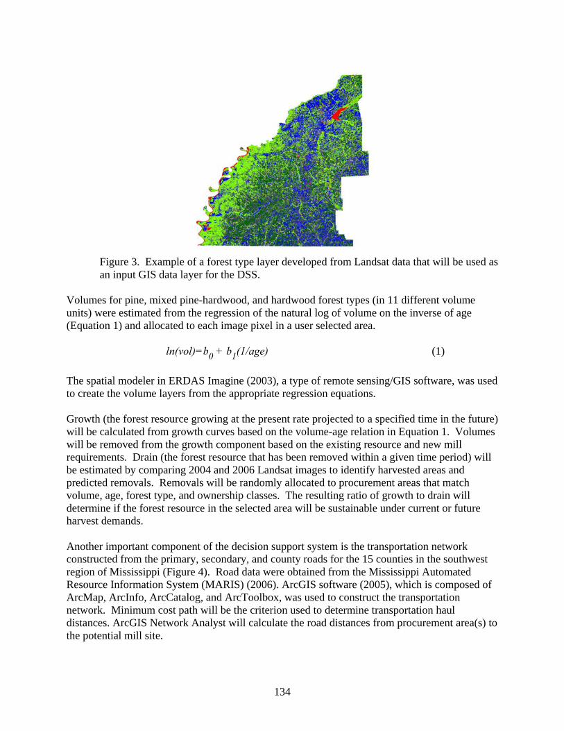
134

Figure 3. Example of a forest type layer developed from Landsat data that will be used as an input GIS data layer for the DSS.

Volumes for pine, mixed pine-hardwood, and hardwood forest types (in 11 different volume units) were estimated from the regression of the natural log of volume on the inverse of age (Equation 1) and allocated to each image pixel in a user selected area.

ln(vol)=b0 + b1(1/age) (1) The spatial modeler in ERDAS Imagine (2003), a type of remote sensing/GIS software, was used to create the volume layers from the appropriate regression equations. Growth (the forest resource growing at the present rate projected to a specified time in the future) will be calculated from growth curves based on the volume-age relation in Equation 1. Volumes will be removed from the growth component based on the existing resource and new mill requirements. Drain (the forest resource that has been removed within a given time period) will be estimated by comparing 2004 and 2006 Landsat images to identify harvested areas and predicted removals. Removals will be randomly allocated to procurement areas that match volume, age, forest type, and ownership classes. The resulting ratio of growth to drain will determine if the forest resource in the selected area will be sustainable under current or future harvest demands. Another important component of the decision support system is the transportation network constructed from the primary, secondary, and county roads for the 15 counties in the southwest region of Mississippi (Figure 4). Road data were obtained from the Mississippi Automated Resource Information System (MARIS) (2006). ArcGIS software (2005), which is composed of ArcMap, ArcInfo, ArcCatalog, and ArcToolbox, was used to construct the transportation network. Minimum cost path will be the criterion used to determine transportation haul distances. ArcGIS Network Analyst will calculate the road distances from procurement area(s) to the potential mill site.

135

Figure 4. Example of the transportation network constructed for 15 counties in the southwest inventory region of Mississippi that will calculate the shortest distance between a procurement area(s) (#1) and a potential mill site (#2).

Once the growth and drain ratio, procurement costs, and transportation costs are determined, a linear programming model for determining the optimal location of a mill to minimize costs will be constructed using C-whiz software (2003). The objective function will minimize the costs of procuring wood for a potential mill site and transporting the finished product to market. Input variables and constraints that will be used are those used by McCauley and Caulfield (1990) (Tables 1 and 2, respectively). Sensitivity analyses will identify the LP factors with the greatest influence on mill location, such as stumpage volume, timber type, size class, and ownership class. Mill feasibility will be assessed by calculating net present values (NPV). All the components of the optimal mill location and suitability DSS will be combined in a seamless Microsoft Visual C++ (2005) interface and linked to the current MIFI interface, http://www.mifi.ms.gov/mission.htm, (Figure 5). Table 1. Constraints that will be used in the LP model that minimizes the costs of procuring wood to the potential mill site and transporting the finished product to market (after McCauley and Caulfield 1990).

-A binary constraint to show that a certain number of plants are located -A wood requirement -One that makes sure the mill does not exceed the amount of timber available in a region -One that shows the production requirement of the proposed mill -One that does not let the quantity of the finished product shipped to a specific market location exceed the demand -One that limits the proportion of mill furnish (pine/hardwood) used in production -A nonegativity constraint

!1

!2!2#1 #2

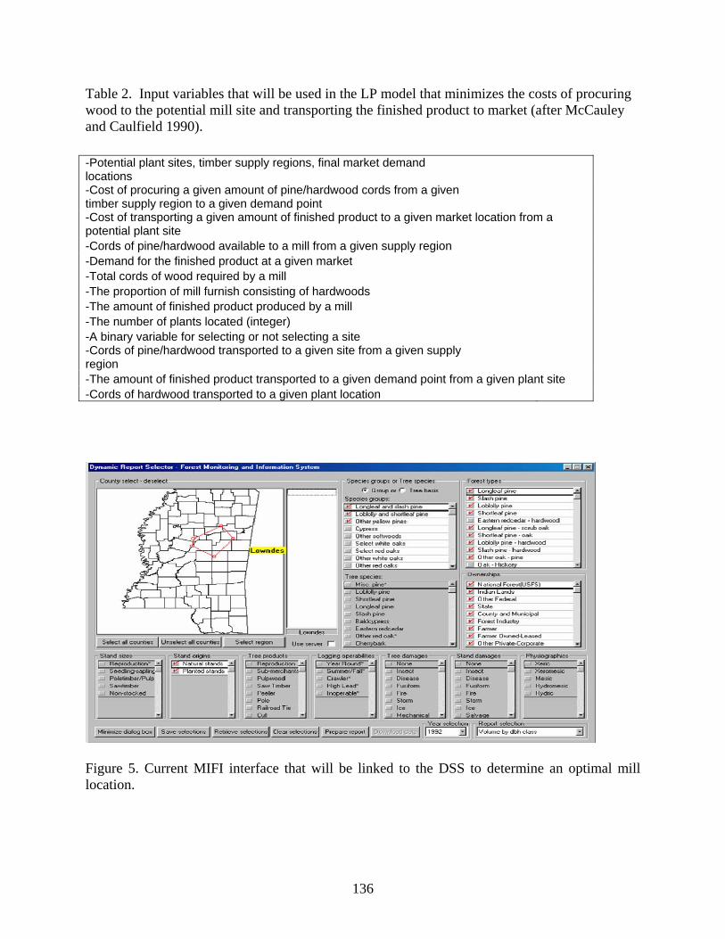
136

Table 2. Input variables that will be used in the LP model that minimizes the costs of procuring wood to the potential mill site and transporting the finished product to market (after McCauley and Caulfield 1990).

Figure 5. Current MIFI interface that will be linked to the DSS to determine an optimal mill location.

-Potential plant sites, timber supply regions, final market demand locations -Cost of procuring a given amount of pine/hardwood cords from a given timber supply region to a given demand point -Cost of transporting a given amount of finished product to a given market location from a potential plant site -Cords of pine/hardwood available to a mill from a given supply region -Demand for the finished product at a given market -Total cords of wood required by a mill -The proportion of mill furnish consisting of hardwoods -The amount of finished product produced by a mill -The number of plants located (integer) -A binary variable for selecting or not selecting a site -Cords of pine/hardwood transported to a given site from a given supply region -The amount of finished product transported to a given demand point from a given plant site -Cords of hardwood transported to a given plant location

137

Anticipated Impact The DSS will fill a critical role in assessing the current and future availability and costs of forest resources within user defined regions of Mississippi. The results of forecasting future raw material availability should be used to assess the need for forest landowner educational and incentive programs in reforestation, management, and utilization, ensuring a sustainable supply and reducing the risk of mill failures. Lawmakers will have information upon which to base policy decisions guaranteeing the environmental and economic sustainability of the forest lands that support a major component of the State’s economic base. Forest land managers will possess the best possible information to evaluate economic risk for new and existing plants. An effective, Web-based, easy-to-use presentation of the complex models associated with the DSS will empower its use by forest managers, policy makers, and foresters. The final product will be a monumental step forward in automating the process of evaluating forest-based resource supply and mill feasibility. The system will provide a framework for gathering and organizing the essential data that has, in the past, been manually prepared. Manual preparation involves numerous consultants (experts), and is very costly and error prone. This DSS will incorporate the most recent and precise inventory information and expert knowledge making that knowledge readily available to users in an effective, low cost, and timely manner. The ultimate impacts are: 1) the promotion of stand management and reforestation, 2) more efficient utilization of the resource, and 3) the prevention of over-utilization of the resource and environmental degradation. . Literature Cited ESRI. 2005. ArcGIS Software, Version 9.1. Redlands, CA. KMS Optimization Products, The Bionetics Corporation. 2003. C-whiz, Version 4, Linear

Programming Optimizer. Arlington, VA: Ketron Management Science User’s Reference Manual, 126 pp.

Leica Geosystems GIS and Mapping. 2003. ERDAS Imagine, Version 8.7. Norcross, GA. McCauley, K.C. and J.P. Caulfield. 1990. Using mixed-integer programming to determine the optimal location for an oriented strandboard plant in Alabama. Forest Products

Journal. 40(2): 39-44. Microsoft. 2005. Microsoft Visual Studio 2005. Redmond, WA Mississippi Automated Resource Information System. 2006. Primary, Secondary, and County

road files, Acquired electronically May 2006. Jackson, MS Munn, I.A. and B.K. Tilley. 2005. Forestry in Mississippi: The impact of the forest products

industry on the Mississippi economy, an input output analysis. Forest and Wildlife Research Center, Bulletin FO301, Mississippi State University. 27 pp.

138

Sun, C. and D. Zhang. 2001. Forest resources, government policy, and investment location decisions of the forest products industry in the southern United States. Forest Science. 47(2): 169-177.

139

Logging Residues as a Source of Bioenergy Feedstock

Robert K. Grala1, 2, Laura A. Grace2, and William B. Stuart2

Abstract: High oil prices and energy security resulted in increased interest in renewable sources of energy such as biomass. A recent goal of replacing 30% of current US petroleum consumption with biomass-derived fuels, set by a joint committee of US Department of Energy and Department of Agriculture, will require annually 1.5 billion tons of biomass originating mostly from agricultural and forest sectors. Mississippi forest sector can contribute significantly to the achievement of this goal. Currently, majority of forest-based biomass feedstock is derived from mill residues, pulping liquors and fuelwood. However, utilization rate of processing residues is relatively high leaving little room for further improvements. Harvesting operations generate significant amount of logging residues that are usually left unused in the forest. Utilization of this biomass source has been limited, primarily due to prohibitive harvesting and transportation costs. However, more efficient harvesting and transportations systems, and improved logistics might enable more effective utilization of these resources. This research project examines feasibility of increasing quantity of woody feedstock through improved recovery of logging residues. Distribution and accessibility of logging residues in Mississippi is evaluated. Maximum hauling distances to processing facilities are established and quantities of residues that can be recovered cost effectively are determined. Keywords: Bioenergy, harvesting, logging residues, transportation, woody biomass.

1 Corresponding author, rgrala@CFR.MsState.Edu, (662) 325-7039 (v). 2 Department of Forestry, Mississippi State University, Box 9681, Mississippi State, MS 39762-968.

140

To Burn or Not to Burn

Sun Joseph Chang1

Abstract: Every year, roughly 7 million tons of bagasse were produced in the US South as a by-product of sugar production from sugar cane. These fibers represent an attractive source of raw material for either pulp production or cellulosic bio-ethanol production. In this paper we will present the results of a recent study of their availability and the economics of burning as opposed to using the fiber for other purposes.

1 Professor, School of Renewable Natural Resources, Louisiana State University, Baton Rouge, LA 70803, xp2610@lsu.edu.

141

Economic Impacts Associated with Mississippi Outfitters and Their Clientele

Anwar Hussain and Ian A. Munn1

Abstract: Outfitter enterprises and their clientele play an important role in regional economies. Based on a survey data of Mississippi outfitters and their clientele, we simulated impacts induced by their direct expenditures on industry output, value added and employment generation at the state level and by species type (white-tailed deer - Odocoileus virginianus, quail - Colinus virginianus, and waterfowl - Anas spp.). Results suggested that outfitter-associated expenditures generated US$9.67 million in value added and 250 full or part-time jobs, whereas clientele-associated expenditures generated US$1.33 million and 42 full or part-time jobs. By conservative estimate, the Mississippi outfitter activities constitute a 10 million dollar industry. These results may be helpful to planners and policy makers as they weigh the role of alternative regional development strategies. Keywords: Input-output analysis, IMPLAN, natural resource-based development, recreation

1 Assistant Research Professor and Professor, respectively, Forestry Department, Forest and Wildlife Research Center, Mississippi State University, imunn@CFR.MsState.Edu, (662) 325-4546 (v).

142

Economic Impacts of Two Birding Festivals in Mississippi*

Marcus K. Measells1 and Stephen C. Grado2

Abstract: Birdwatching is a recreational activity that has continually been gaining popularity in the United States. The Great River Birding Trail (GRBT) research project being conducted at Mississippi State University will measure current and potential social and economic impacts of birdwatching on private and public sites along the GRBT in Mississippi. This paper focused on expenditure data and economic impacts from birding festivals. On-site interviews were conducted in 2006 at two festivals: one hosted by TARA Wildlife and the other by Audubon Mississippi. Economic impacts were modeled using the Impact Analysis for Planning (IMPLAN) System software. The three-day Stork and Cork festival at TARA Wildlife had 145 individuals in attendance with a total economic impact of $10,031. The four-day Hummingbird Migration Celebration was attended by 7,970 individuals resulting in a total economic impact of $97,654. Information from this study will assist natural resource and tourism agencies and non-governmental organizations as they attempt to complete the Trail along the Lower Mississippi River. It will also allow rural land planners and policy makers to estimate benefits accrued from various land management alternatives on areas related to the Trail and will be useful for establishing marketing and policy strategies related to eco-tourism and resource management oriented toward birdwatching. Keywords: Birdwatching, economic impacts, expenditures, Great River Birding Trail, nature tourism, on-site surveys Introduction Mississippi is a state endowed with a wealth of natural resources. Among these are its avian resources, which have increasingly been utilized not only for hunting, but also for insect control, ecological diversity, and recreation-related activities such as birdwatching and wildlife photography. An assumption can be made that birdwatching is an important component of eco-tourism. Therefore, proper avian resource management should be of utmost importance to private and public landowners and natural resource and tourism agencies. One component of this overall effort in Mississippi is the Great River Birding Trial (GRBT). Currently, there is a self-guided birding tour on the northern reaches of what is one of America's longest birding trails. The GRBT is named after the federally designated scenic drive called the Great River Road, which runs from Canada to the Gulf of Mexico. In general, the sites along the Trail include established * Special thanks to the staff at Audubon Mississippi, TARA Wildlife, and Strawberry Plains Audubon Center for allowing us to conduct this study. This manuscript is publication No. FO341 of the Forest and Wildlife Research Center, Mississippi State University. 1 Research Associate II, Mississippi State University, Forest and Wildlife Research Center, College of Forest Resources, Box 9681, Mississippi State, MS 39762, marcm@ext.msstate.edu, (662) 325-3550 (v), (662) 325-8726 (fax). 2 Professor, Mississippi State University, Forest and Wildlife Research Center, College of Forest Resources, Box 9681, Mississippi State, MS 39762.

143

wildlife refuges, parks, overlooks, and other attractions no more than 25 to 30 miles from the Great River Road. Currently, GRBT parallels both sides of the upper Mississippi River from the headwaters at Lake Itasca, Minnesota, downstream for 1,366 miles to the confluence with the Ohio River at Cairo, Illinois. It covers both sides of the upper Mississippi River through Minnesota, Wisconsin, Iowa, Illinois, and Missouri. The next step in the process of completing GRBT is to extend it along both sides of the Lower Mississippi River to the Gulf of Mexico. The driving forces behind this effort are Audubon Mississippi and the U.S. Fish and Wildlife Service. Together, they have identified and delineated birdwatching sites (approximately 300) and pinpointed bird species of interest (T. Pullen, Audubon Mississippi Contract Employee, pers. comm., 2005). Currently, 2/3s of these sites are open to the public with 95% of them public and only 5% private. Audubon Mississippi would like to increase private landowner participation on this portion of the GRBT (T. Pullen, Audubon Mississippi Contract Employee, pers. comm., 2005). However, to accomplish this and promote the GRBT in general, they currently do not have any information on potential economic impacts to compliment what they are trying to achieve (M. Lindsey, Executive Director, Audubon Mississippi, pers. comm., 2005). Without this information as a framework, it will be difficult to evaluate the importance of private landowners in providing birdwatching opportunities to the public. This aspect of the project has both significant social and economic implications that could determine the GRBT’s success. This information will also provide a monetary measure of return to county economies from the retention, improvement, or expansion of avian habitats. Thus, economic and socio-demographic assessments of birdwatching activities are extremely important to the promotion and development of the GRBT in the future. Birding, or birdwatching, is a recreational activity gaining popularity around the United States. Kerlinger (1992) reported that in 1970 only about 4% of Americans were considered birdwatchers; however, by the mid-1980s 25% were considered birders. As of 1995, the number of birdwatchers nationwide increased by 27% and by 225% since 1982 (Scott and Thigpen 2003). Kerlinger (1992) also stated that fewer than 10 site-specific studies of birders had been completed worldwide at that time. To highlight the importance of birdwatching to local economies, he provided the example of Cape May, New Jersey where $6 to 10 million dollars were spent on an annual basis. Crandall et al. (1992) reported approximately 38,000 people visited two conservation areas in southeast Arizona between July 1991 and June 1992 and spent $1.6 million. In a later study, Kerlinger et al. (1997) reported that birders spent between $100 to $130 per day while touring for birds. This amount did not include their travel expenses to and from an area. When trip-related expenses and other expenses such as durable goods were considered, the ensuing expenditures, and hence economic impacts, could be sizable. For example, it was determined that an estimated economic impact of $90 million per year was attributed to birders in the Rio Grande Valley of South Texas (Kerlinger et al. 1997). Nationwide, 66.1 million U.S. residents participated in wildlife-watching activities (USDI and USDC 2002a). Of the 21.8 million participants who observed wildlife away from home: 10.6 million went to public areas only, 2.5 million visited private areas only, and 6 million visited both public and private areas (USDI and USDC 2002a). There is a strong indication that individuals were searching for both public and private locations for wildlife-watching activities. Nearly 46 million of these wildlife watchers observed birds around their homes and on trips in

144

2001 (USDI and USDC 2002a). Beyond natural settings and habitats, other avian-related activities are also important. For example, Waldrup (1994) reported that 40,000 people participated nationwide in the annual Christmas Bird Count. Nationwide, wildlife watchers, 16 years and older, spent $38.4 billion which included equipment expenditures of $23.5 billion, trip-related expenses of $8.2 billion, and other expenditures of $6.7 billion (USDI and USDC 2002a). In 2001, wildlife watchers, 16 years and older, many of whom were birdwatchers (427,000), spent $304 million dollars in Mississippi (USDI and USDC 2002b). Expenditures represent dollars spent in an economy of interest; however, economic impacts measure dollars that remain in that economy. Economic impacts, examined through input-output analysis, are especially useful in describing current and potential economic contributions of natural resource-based recreational activities (e.g., birdwatching) to the overall economy (Johnson and Moore 1993, Strauss et al. 1995, Grado et al. 2001). Economic impacts are often modeled using the Impact Analysis for Planning (IMPLAN) System software (Olson and Lindall 2000). These studies provide regions and states with useful information about the social and economic effects of proposed new projects, programs, and current activities (i.e., birdwatching) (Loomis and Walsh 1997). In 1991, five southern states (Alabama, Arkansas, Louisiana, Mississippi, and Tennessee) generated $270.2 million in retail sales for non-consumptive bird use (Bird Conservation 1997). Mississippi’s portion accounted for $34.9 million; however, this still led to approximately 1,200 full- and part-time jobs in Mississippi supported by non-consumptive bird use (Bird Conservation 1997). This could be due to the lack of birding festivals and established birdwatching locations within Mississippi. One purpose of this overall research project is to increase this number, especially by taking advantage of the large private landownership in the State. As important as birdwatching expenditures are, it is paramount to understand the residence and demographics of birdwatchers. This is of great value when determining advertising and marketing strategies. Hvenegaard (2002) studied birders in Thailand and determined there were three specialization levels among them that included novice, advanced-active, and advanced-experienced birders. Hvenegaard (2002) stated that understanding the demographics of birders will allow for improving economic impacts, developing effective communication and educational programs, and implementing effective marketing campaigns for birders. For example, more advanced birders were more interested only in birding activities (Hvenegaard 2002). Most birdwatchers (97%) in South Carolina prefer to enjoy birdwatching within the state (South Carolina Department of Parks, Recreation, and Tourism 2001). The average South Carolinian went birdwatching 63 times per year, ranking second only to walking as the most favored recreational activity (South Carolina Department of Parks, Recreation, and Tourism 2001). In 1992, birders who were readers of the American Birds magazine were almost evenly split between males and females, 70% attended college, and had a median household income 35% greater than the general public (Waldrup 1994). Average birders at wildlife refuges were middle-aged, highly educated, and had higher than average incomes (Kerlinger et al. 1997). The first objective of this paper was to determine birdwatching expenditures of participants at two birding festivals in Mississippi. The second objective was to quantify the current and potential economic impacts of birding festivals along the GRBT on the Mississippi economy.

145

Methods Dillman (2000) found face-to-face and telephone surveys more popular than mail surveys because they provided more accurate data. Consequently, on-site, face-to-face interviews were used to gather information from birders at two birdwatching festivals to achieve higher response rates and more reliable data. This survey method allowed the interviewer to explain and interpret any questions the interviewee might have about the survey process. These were important considerations when using a detailed survey associated with expenditure data collection. Two birding festivals were held in Mississippi in the fall of 2006. The Stork and Cork Mississippi River Birding Festival was hosted on August 25-27, 2006, at TARA Wildlife (a private entity) located 30 minutes northwest of Vicksburg. The Hummingbird Migration Celebration was hosted on September 7-10, 2006, by Audubon Mississippi at Strawberry Plains Audubon Center (a non-governmental organization) located north of Holly Springs. Face-to-face surveys were conducted on Saturday, August 26 at the Stork and Cork Mississippi River Birding Festival and on Saturday, September 9, 2006, at the Hummingbird Migration Celebration. Survey questions pertained to birding or other activity-related expenditures and birding habits during the year. Participants were asked to provide their on-site, trip-related, and equipment expenditures and the purchase location. In-state expenses were cataloged by amount and county of purchase, and out-of-state expenses by amount and state of purchase. Participants were asked to provide on-site and trip-related expenditures for the current 24 hours to minimize recall error. In situations where participants were on day trips, they were asked to estimate their trip expenses for the remainder of the day. Equipment expenditures included durable items related to participation at the site and acquired during the past year. An estimate on annual use for durable items for all purposes was also collected. Expenses were recorded by specific expenditure category to align them with the corresponding industrial sector in the modeled economy. Long-term expenses were divided by number of days of use for the item during the year. Economic impacts of birding-related activities were modeled using IMPLAN. This software package has been used extensively to study economic impacts of activities related to forestry, agriculture, recreation, tourism, commercial development, and the commercial endeavors of specific industries (Olson and Lindall 2000). IMPLAN software uses economic data from an area of interest to construct a model of its economy. Associated databases provide information required to construct regional or state IMPLAN models (Olson and Lindall 2000). County and state level models define relationships between industries and account for monetary leakages (i.e., business transactions) outside of an economy of interest. These data sets were used to analyze the state input-output structure. Expenditures made on behalf of birding-related activities were then organized as final demands on state industries and businesses. The IMPLAN model was built to identify direct and secondary impacts resulting from birdwatcher expenditures. Direct impacts represented that portion of expenditures retained by an economic entity in the operation of its business such as sales, salaries, wages, and jobs created by initial purchases of participants. Secondary impacts included indirect effects of inter-industry trade within the region and the induced effects of household consumption originating from employment tied to the direct and indirect activities. Economic impacts were measured in terms

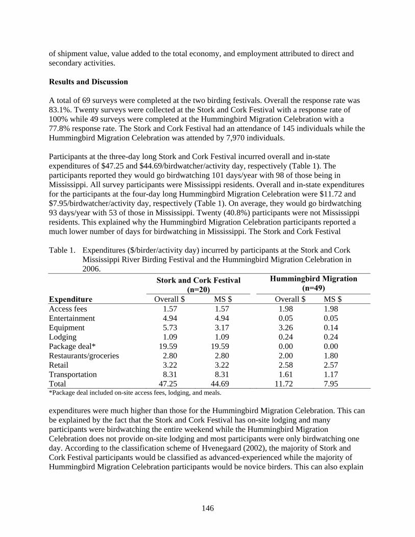
146

of shipment value, value added to the total economy, and employment attributed to direct and secondary activities. Results and Discussion A total of 69 surveys were completed at the two birding festivals. Overall the response rate was 83.1%. Twenty surveys were collected at the Stork and Cork Festival with a response rate of 100% while 49 surveys were completed at the Hummingbird Migration Celebration with a 77.8% response rate. The Stork and Cork Festival had an attendance of 145 individuals while the Hummingbird Migration Celebration was attended by 7,970 individuals. Participants at the three-day long Stork and Cork Festival incurred overall and in-state expenditures of $47.25 and $44.69/birdwatcher/activity day, respectively (Table 1). The participants reported they would go birdwatching 101 days/year with 98 of those being in Mississippi. All survey participants were Mississippi residents. Overall and in-state expenditures for the participants at the four-day long Hummingbird Migration Celebration were $11.72 and $7.95/birdwatcher/activity day, respectively (Table 1). On average, they would go birdwatching 93 days/year with 53 of those in Mississippi. Twenty (40.8%) participants were not Mississippi residents. This explained why the Hummingbird Migration Celebration participants reported a much lower number of days for birdwatching in Mississippi. The Stork and Cork Festival Table 1. Expenditures ($/birder/activity day) incurred by participants at the Stork and Cork

Mississippi River Birding Festival and the Hummingbird Migration Celebration in 2006.

Stork and Cork Festival

(n=20) Hummingbird Migration

(n=49) Expenditure Overall $ MS $

Overall $ MS $ Access fees 1.57 1.57 1.98 1.98 Entertainment 4.94 4.94 0.05 0.05 Equipment 5.73 3.17 3.26 0.14 Lodging 1.09 1.09 0.24 0.24 Package deal* 19.59 19.59 0.00 0.00 Restaurants/groceries 2.80 2.80 2.00 1.80 Retail 3.22 3.22 2.58 2.57 Transportation 8.31 8.31 1.61 1.17 Total 47.25 44.69 11.72 7.95 *Package deal included on-site access fees, lodging, and meals. expenditures were much higher than those for the Hummingbird Migration Celebration. This can be explained by the fact that the Stork and Cork Festival has on-site lodging and many participants were birdwatching the entire weekend while the Hummingbird Migration Celebration does not provide on-site lodging and most participants were only birdwatching one day. According to the classification scheme of Hvenegaard (2002), the majority of Stork and Cork Festival participants would be classified as advanced-experienced while the majority of Hummingbird Migration Celebration participants would be novice birders. This can also explain

147

the difference in expenditures as the advanced-experienced birders were willing to spend more of their money on their birdwatching activities. Economic impacts resulting from the two birdwatching festivals were reported for direct sales, indirect sales, induced sales, and total sales for aggregated sectors within the economy (Tables 2 and 3). Total direct sales from the two festivals in 2006 were $71,513. This stimulated secondary sales (indirect and induced) of $36,172, allowing the total sales impacts to reach $107,685 and supporting 1.6 full- and part-time jobs. The major beneficiaries of birdwatching expenditures were the aggregated sectors of manufacturing and services.

Table 2. Total economic impacts of birdwatchers at the Stork and Cork Mississippi River

Birding Festival, August 25-27, 2006. Industry Direct ($) Indirect ($) Induced ($) Total ($) Ag., For., Fisheries 0 26 31 58 Mining 0 208 69 278 Construction 0 0 1 1 Manufacturing 2,072 775 879 3,725 TCPUa 0 122 48 170 Trade 0 157 32 189 FIREb 0 34 23 57 Services 4,545 183 826 5,553 Total 6,616 1,506 1,909 10,031 aTransportation, communication, and public utilities. bFinance, insurance, and real estate. Table 3. Total economic impacts of birdwatchers at the Hummingbird Migration Celebration,

September 7-10, 2006. Industry Direct ($) Indirect ($) Induced ($) Total ($) Ag., For., Fisheries 0 309 319 628 Mining 0 1,659 702 2,361 Construction 0 2 5 7 Manufacturing 33,473 7,265 8,916 49,654 TCPUa 0 932 486 1,418 Trade 0 1,460 325 1,785 FIREb 0 276 235 511 Services 31,424 1,489 8,377 41,289 Total 64,897 13,392 19,365 97,654 a Transportation, communication, and public utilities. b Finance, insurance, and real estate.

As this research project continues, additional surveys will be conducted at other birdwatching festivals and events. This information will be combined with birdwatching expenditures gathered from a set of public and private sites, already established or under construction along the GRBT, as well as with operator site expenditures. This additional information will allow for a more detailed and accurate determination of the overall economic impact of all birdwatching activities along the GRBT. The results of this study can be used by Audubon Mississippi and other public

148

agencies to promote the further development of birdwatching sites on both public and privately held lands along the GRBT. Additionally, state and federal agencies, conservation groups, private businesses, and landowners can improve local economies by marketing and planning improvements and developments that enhance birding resources (e.g., bird habitat, birdwatching facilities, bird species sustainability) based on economic impact analysis. An improved marketing strategy will increase awareness among birders nationwide about unique birding opportunities available in Mississippi and help increase the number of birding activities and events in the State, resulting in enhanced economic impacts. Conclusions Information from this study will assist natural resource (e.g., U.S. Fish and Wildlife Service) and tourism agencies (e.g., Mississippi Division of Tourism) and non-governmental organizations (e.g., Audubon Mississippi, The Nature Conservancy) in their efforts to complete the GRBT in the Lower Mississippi River area. Also, connecting to the work already accomplished in the Upper Mississippi River area and the Mississippi Coastal Birding Trail will be an invaluable asset for Mississippi and other states in the Lower Mississippi River area. Quantifying total employment, income, value added, taxes, and total sales will allow natural resource and tourism agencies, land use planners, and policy makers to estimate benefits accrued from various land management options related to birdwatching both on areas related to the GRBT and beyond. On this basis, funding for birdwatching area restoration, species sustainability, and tourism promotion can be justified from both a biological and economic standpoint. The information will also be useful for establishing marketing and policy strategies related to eco-tourism and resource management oriented toward birdwatching and to garner legislative support for funding initiatives to address specific study areas for the GRBT. Literature Cited Bird Conservation. 1997. What’s a bird worth? Bird Conservation 6-8. Crandall, K., J. Leones, and B.G. Colby. 1992. Nature-based tourism and the economy of

southeastern Arizona: Economic impacts of visitation to Ramsey Canyon Preserve and San Pedro Riparian National Conservation Area. Tucson: University of Arizona.

Dillman, D.A. 2000. Mail and internet surveys: The tailored design method. 2nd edition. Wiley

and Sons, Inc., New York, New York. 464pp. Grado, S.C., R.M. Kaminski, I.A. Munn, and T.A. Tullos. 2001. Economic impact of waterfowl

hunting on public lands and at private lodges in the Mississippi Delta. Wildl. Soc. Bulletin 29(3):846-855.

Hvenegaard, G.T. 2002. Birder specialization differences in conservation involvement,

demographics, and motivations. Human Dimensions of Wildl. 7:21-36.

149

Johnson, R.L. and E. Moore. 1993. Tourism impact estimation. Annals of Tourism Res. 20:279-288.

Kerlinger, P. 1992. Birding economics and birder demographics studies as conservation tools. In:

Status and management of neotropical migratory birds. D.M. Finch and P.W. Stangel, Eds. Gen. Tech. Rep., RM 229, pp. 32-38.

Kerlinger, P., R.H. Payne, and T. Eubanks. 1997. Not just for the birds: New studies demonstrate

that wildlife refuges can be a financial boon for nearby communities. Bird Conservation 12-13.

Loomis, J.B. and R.G. Walsh. 1997. Recreation economic decisions: Comparing benefits and

costs. Venture Publishing, Inc., State College, Pennsylvania. Olson, D. and S. Lindall. 2000. IMPLAN Professional. 2nd ed. MIG, Co., Stillwater, Minnesota. Scott, D. and J. Thigpen. 2003. Understanding the birder as tourist: Segmenting visitors to the

Texas hummer/bird celebration. Human Dimensions of Wildl. 8:199-218. South Carolina Department of Parks, Recreation, and Tourism. 2001. Birding and other wildlife

watching: An overview of the demographics, economics, and trends of wildlife watching, including birdwatching, in South Carolina and the United States. South Carolina Department of Parks, Recreation, and Tourism. Columbia, South Carolina. 4 pp.

Strauss, C.H., B.E. Lord, and S.C. Grado. 1995. Economic impact of travel and tourism in

Southwestern Pennsylvania during 1994. School of Forest Resources, Pennsylvania State University, University Park, Pennsylvania.

U.S. Department of the Interior and U.S. Department of Commerce (USDI and USDC). 2002a.

2001 National Survey of Fishing, Hunting, and Wildlife-Associated Recreation. U.S. Dep. Int., Fish and Wildlife Serv., and U.S. Dep. Comm., Bur. Census. U.S. Gov. Printing Office, Washington, D.C., 116 pp.

U.S. Department of the Interior and U.S. Department of Commerce (USDI and USDC). 2002b.

2001 National Survey of Fishing, Hunting, and Wildlife-Associated Recreation-Mississippi. U.S. Dep. Int., Fish and Wildlife Serv., and U.S. Dep. Comm., Bureau of Census. U.S. Gov. Printing Office, Washington, D.C., 46 pp.

Waldrop, J. 1994. For the birds. American Demographics 16(1):4.

150

An Introduction to the Southern US Wood Supply System: A Value Chain Approach*

Clayton B. Altizer1 Abstract: Much of the economic activity generated by timber harvesting contributes heavily to local and regional economies and the subsequent currency turnover in such communities is high. Value chains are the “other side” of the supply chain, responsible for distributing elements of value back to the suppliers of those goods and services. With a supply chain, it is much easier to identify stakeholders and attach appropriate responsibilities and degrees of separation. A well-constructed value chain is much more complex and the economic and social interactions are more difficult to trace. The value chain for forestry usually extends completely across the physical and political landscape, reaching in to most geographically and economically remote locations. Traditional emphasis has been on only two segments of the value chain, timber growers and converting firms. The intermediate enterprises and participants have been considered mere producers of service, therefore largely “outside” the system. Often, businesses of this ilk are viewed as expendable and the socioeconomic contributions or benefits they offer within their respective communities are frequently discounted, ignored, or lost. This research addresses this void by proposing a model to adequately represent the complexity of the wood supply value chain. Keywords: Timber harvesting, conceptual model Introduction Production forestry plays a vital role in the economic development of the southern US. Munn and Tilley (2005) state that over $1 billion worth of forest products are harvested from Mississippi’s forest lands annually, with timber harvesting currently generating over 11,000 jobs. This influx of revenue is divided among the key players in the wood supply system (forest landowners, loggers, and consuming mills) with much of the economic benefits staying in local coffers while some of this revenue leaves local, state, and regional jurisdictions. A well constructed value chain model is beneficial for depicting these interactions and demonstrating how important production forestry is for the livelihood of rural southern communities. In many instances, a mill closure and the subsequent job loss for such communities has devastating effects. The social and economic impacts of these unfortunate events are widespread and long-term in nature. A better understanding and appreciation of the entire process is paramount for all stakeholders involved in the wood supply system. * Approved for publication as manuscript number FO338 of the Forest and Wildlife Research Center, Mississippi State University. The author would like to acknowledge Dr. Laura A. Grace, Dr. William B. Stuart, Dr. Robert K. Grala, Dr. Anwar Hussain, and Dr. William D. Eshee, Jr., all faculty members at Mississippi State University, for their leadership and contributions to this research effort. This research was supported by The Forest and Wildlife Research Center (FWRC) - Mississippi State University, The USDA Wood Utilization Research (WUR) Program, and The Wood Supply Research Institute (WSRI). 1 Research Associate II, Department of Forestry, Mississippi State University, Box 9681, Mississippi State, MS, 39762, caltizer@cfr.msstate.edu, (662) 325-8027 (v), (662) 325-8027 (fax).

151

Current Wood Supply System The wood supply system in the southern US is comprised of 3 primary stakeholders: the landowner, the logger, and the consuming mill. One of the social and economic dilemmas facing production forestry today is that the relationships between the key players in the wood supply system are poorly understood and not well documented. Research has traditionally focused on growth and increasing yield of individual trees or stands, or on the finished product once the raw material arrives at the manufacturing plant. The broad area consisting of harvesting timber and transporting this raw material to the consuming mills has generally been taken for granted and largely ignored. This process is critical to the field of forestry and forest products, and has a myriad of social and economic impacts for society as a whole. This is precisely the reason that the development of a wood supply value chain is imperative to the overall health of the industry. The Wood Supply Research Institute (WSRI) and Mississippi State University researchers have acknowledged the importance of maintaining the structural integrity of the system and have responded by placing an increased emphasis on examining the timber harvesting component of the overall system. This collaboration has produced a series of reports documenting some alarming trends afflicting the current health and status of the logging profession. Most notably, the long-term logging cost index developed through this research effort has documented a 42 % increase in the overall total price per delivered ton of wood fiber using 1995 as a base year for the index (Stuart et al. 2007). When compared to the consumer price index (CPI) and the producer price index for logging services (PPIL), both indices produced by the US Department of Labor – Bureau of Labor Statistics, an even more troubling trend is apparent. For 2005, the WSRI logging cost index is 12 % higher than the consumer price index; the largest disparity between the two figures for the entire 10-year study period (Stuart et al. 2007). The consumer price index is the price a consumer pays for a myriad of essential goods and services and is commonly used as an indicator of cost of living and/or inflation. Stuart et al. (2007) further contend that a 52 point divergence is apparent for 2005 between the WSRI logging cost index and the producer price index for logging services (the price paid for logging services). In fact, the price paid for logging services has decreased 10 % since the base year of 1995. Supply Chains vs. Value Chains The focus on supply chain relationships and management in the forest products industry and wood supply system has been economic in nature, and generally centered on the wood consumer. Meeting production demands and ensuring that certification guidelines are met are common supply chain models. Traditional emphasis has been on only two segments of the system: the growers and the converting firms. The intermediate enterprises and participants have been considered mere service providers, therefore largely “outside” the system. Very little emphasis has been placed on examining social and policy relationships, and responsibilities associated with conversion from the stump to the finished product.

152

According to Beamon (1998), “a supply chain may be defined as an integrated process wherein a number of various business entities (i.e., suppliers, manufacturers, distributors, and retailers) work together in an effort to: (1) acquire raw materials, (2) convert these raw materials into specified final products, and (3) deliver these final products to retailers”. This chain is typically depicted as a forward flow of materials and a backward flow of finances and information. This backward flow is the framework for a value chain. Value chains are the “other side” of the supply chain, responsible for distributing elements of value back to the suppliers of those goods and services. Supply chains are used more frequently than value chains even though the terms are often used interchangeably. Neither is commonly used in describing the wood supply system. They are more common in the field of agricultural economics, specifically in relation to topics directly involved in the food chain. Salin (2000) examines the cattle-beef market and focuses on the importance of responsiveness to consumer needs and efficient delivery of goods to consumers. Ward and Stevens (2000) state that for many agricultural products, mainly beef and dairy products, the identity of the initial product remains virtually clear along the distribution chain. For other products, including those manufactured from wood fiber, the identity of the initial product can be “lost” as it is transformed into the finished product. The development of an integrated supply chain requires the management of material and information flows at three levels: strategic, tactical, and operational (Mason-Jones and Towill 1999). These approaches are commonly found in business system engineering designs and information systems. Consumers are becoming more diverse in their demands which have created increased pressures on service industries to provide high quality diversified products at a low cost (Talluri et al. 1999). Modern society has added a forth dimension, that of protecting the environment. Davis (1993) stresses three distinct sources of uncertainty that plague supply chains: suppliers, manufacturing, and customers. Late deliveries from suppliers, machine breakdowns in the manufacturing process, and changing consumer preferences are a few, among many, scenarios that can disrupt the smooth flow of an ideal supply chain. The forestry supply chain is complex beginning with the grower (landowner), the producer (logger), and the supplier (dealer or broker). Chains differ from traditional marketing channels in the degree of cooperation among firms involved in the process (Salin 2000). With a supply chain, it is much easier to identify stakeholders and attach appropriate responsibilities and degrees of separation. A well-constructed value chain is much more complex, and the economic and social interactions are more difficult to trace. For the purposes of simplification, supply chains illustrate the relationships necessary in converting a raw material into a finished merchantable product. On the other hand, value chains depict the entire process in a more 3-dimensional model which encompasses everyone that either contributes or benefits from the process being analyzed.

153

Conceptual Model This research presents a conceptual model depicting the wood supply value chain. All players in the system will be documented and their sphere of influence will be traced throughout the wood supply process. This model should serve as a foundation for a more complex depiction of the wood supply value chain. It should be noted that in reality the stakeholders comprising the model function and interact in a 3-dimensional format. However, to better describe the model and facilitate comprehension, it is unraveled and presented in a 2-dimensional format. Landowners and transportation firms have a vested interest in the process, as do loggers and the consuming mill. It is important that these entities, while sometimes of lower profile, are included in the stakeholder process. Failure to include them results in an incomplete value chain and leads to flawed decision-making. The model constructed quickly evolved into a considerable network and defining it in detail will require additional work. The structure is most easily illustrated by dividing the model into several different sections for discussion, and by following one sample branch of the network. Other branches of the network should be expanded and explored in the same manner. The reader should understand that the model accounts for both direct and indirect relationships at several levels and these relationships extend in both directions. Primary relationships with any entity in the supply chain are those with a direct business relationship, such as between the mill and a chemical or energy supplier or between the logger and a wood dealer. A secondary relationship for the mill is that between a primary supplier or customer and his customer or supplier. A mill, relying on a dealer system for procurement, has a primary relationship with the procurement division of the plant, a secondary relationship with the wood dealer, and a tertiary relationship with the logging contractor supplying wood through that dealer and with the landowner from whom the dealer acquires timber. A fourth level or quaternary relationship is one step further removed. The mill would have a quaternary relationship with the labor force working for the logging contractor, the fuel supplier to that operation, and the equipment dealershipsupplying logging machinery. The grocery store where that worker’s family buys food and the bank that holds their mortgage has a fifth level or quinary relationship with the mill. “Arms length relationship” is a term used to explain legal relationships between separate entities and is commonly used in the wood supply industry (Black 1990). Primary, secondary, tertiary, quaternary, and quinary simply describe how many “arm lengths” separate the entities. These arm lengths form the value chain, and the action of any one of these entities has an effect on the others. That effect may be diminished or amplified by the distance between the two parties. Some actions are diffused as they move down the supply chain while others are amplified. All direct suppliers and customers are stakeholders in the supply chain for they have made an investment of money, skill, energy, and time in the functioning of the process. Process changes and variability have an effect on the viability of those investments. The model can be best understood by selecting a starting point and tracing the multiple direct and indirect relationships through the entire system. The mill was chosen to be the center of the model for this discussion (Figure 1). The choice of the mill as the center is not intended to reflect a placement of importance, but is simply an arbitrary, but important, starting point. Solid

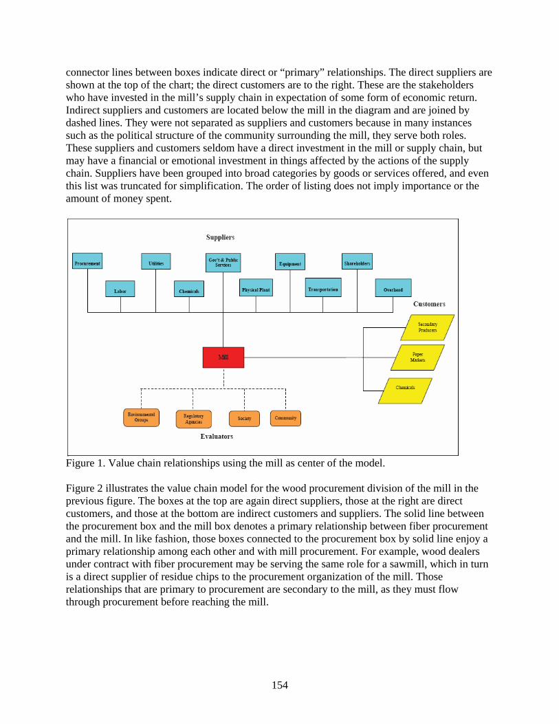
154

connector lines between boxes indicate direct or “primary” relationships. The direct suppliers are shown at the top of the chart; the direct customers are to the right. These are the stakeholders who have invested in the mill’s supply chain in expectation of some form of economic return. Indirect suppliers and customers are located below the mill in the diagram and are joined by dashed lines. They were not separated as suppliers and customers because in many instances such as the political structure of the community surrounding the mill, they serve both roles. These suppliers and customers seldom have a direct investment in the mill or supply chain, but may have a financial or emotional investment in things affected by the actions of the supply chain. Suppliers have been grouped into broad categories by goods or services offered, and even this list was truncated for simplification. The order of listing does not imply importance or the amount of money spent.

Figure 1. Value chain relationships using the mill as center of the model. Figure 2 illustrates the value chain model for the wood procurement division of the mill in the previous figure. The boxes at the top are again direct suppliers, those at the right are direct customers, and those at the bottom are indirect customers and suppliers. The solid line between the procurement box and the mill box denotes a primary relationship between fiber procurement and the mill. In like fashion, those boxes connected to the procurement box by solid line enjoy a primary relationship among each other and with mill procurement. For example, wood dealers under contract with fiber procurement may be serving the same role for a sawmill, which in turn is a direct supplier of residue chips to the procurement organization of the mill. Those relationships that are primary to procurement are secondary to the mill, as they must flow through procurement before reaching the mill.

155

Figure 2. Value chain model for wood procurement division of the mill. The indirect customers and suppliers for fiber procurement fall into the same broad category as for the mill, but are likely quite different groups or segments of larger groups with different or specific interests. Where environmental groups with concerns over air quality and point source water pollution are attracted to the mill, those associated with procurement are more likely to have concerns about endangered species, clearcutting, and non-point source pollution. Figure 3 delves one level deeper in the value chain and shows functional relationships for wood dealers, an example of secondary stakeholders of the mill. The position of the boxes relative to the central wood dealer box is the same as in the previous examples. Independent and contract loggers supplying wood through this dealership have a primary relationship with it, a secondary relationship with procurement, and a tertiary relationship with the mill.

156

Figure 3. Value chain model for wood dealers responsible for supplying harvesting force for the mill. Indirect customers and suppliers again fall into the same broad categories, but operate on a different scale. As the scope of operation becomes more localized, these do as well. At this level, local chapters of larger environmental groups are important, as are relationships with regional planning groups, county government, local newspapers, and civic groups. The cost of meeting the concerns of these groups is more easily identified. Expenditure which is required to meet the concerns of these groups is a part of normal business practice and support the firm’s position in the local business community and forestry community. The potentially larger costs and less predictable costs are those of lost business opportunities and possible legal proceedings if something goes wrong. Figure 4 moves one more link down the chain to the logging contractor, who has a tertiary relationship with the mill. The nature of both direct and indirect customers and suppliers change again. Many of the direct relationships at this level are community based and scattered throughout the procurement region. Labor drawn from the local pool, fuel purchased from a local supplier, and equipment purchased from a local dealer. The nature of the indirect customers and suppliers is also more localized. Public relations may focus on the adjacent landowner, government relations on the county road engineer, and environmental concerns on a specific stream segment or wildlife species. Again, the costs become more concrete. Business opportunities are tied closely with local business reputation. Additional costs are quite often in the form of fines for regulatory violations, performance bonds, permits, and insurance costs.

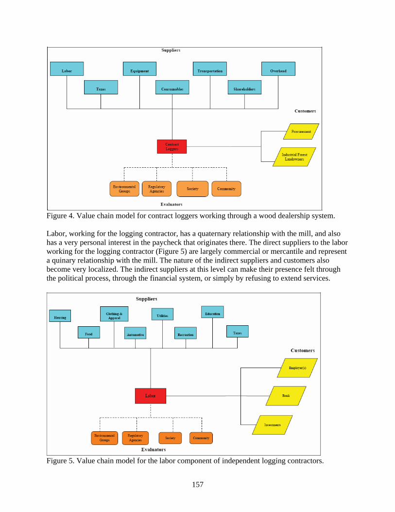
157

Figure 4. Value chain model for contract loggers working through a wood dealership system. Labor, working for the logging contractor, has a quaternary relationship with the mill, and also has a very personal interest in the paycheck that originates there. The direct suppliers to the labor working for the logging contractor (Figure 5) are largely commercial or mercantile and represent a quinary relationship with the mill. The nature of the indirect suppliers and customers also become very localized. The indirect suppliers at this level can make their presence felt through the political process, through the financial system, or simply by refusing to extend services.

Figure 5. Value chain model for the labor component of independent logging contractors.

158

Conclusions Today’s harvesting sector is plagued by drastically increasing operating costs, cash flow problems, and a general uncertainty of future production capacities. The economy of scale principle, which is commonly observed in manufacturing, does not seem to apply to timber harvesting firms. Corporate mergers and acquisitions, as well as constantly changing mill and wood procurement management, have created a cloud of uncertainty regarding the future role of independent contractors in the wood supply system. In this sense, the struggle of farmers trying to provide our country with a steady food supply and independent loggers trying to produce enough raw material to meet our nation’s demand for wood fiber are essentially the same. Likewise many of the problems facing agriculture and production forestry are identical, and both sets of problems have the potential to adversely affect the future roles of each profession. Effective management of the value chain is critical to supply chain management, for if the suppliers of goods and services are not satisfied that they are being properly remunerated, they will withdraw their services. Increasing operating expenses coupled with decreasing prices paid for services rendered affects the entire wood supply system and the ramifications and repercussions can be severe and long-term in nature. The value chains for many industries are relatively short, extending through the town or city where the plant is located. The value chain for forestry usually extends completely across the physical and political landscape, reaching in to the most geographically and economically remote locations. Such complexity warrants further exploration and expansion of this model to accurately depict the wood supply system in detail and the subsequent socioeconomic effects on local and regional communities. Literature Cited Beamon, B.M. 1998. Supply chain design and analysis: Models and methods. Int. J. Prod. Econ.

55: 281-294. Black, H.C. 1990. Black’s Law Dictionary (Sixth Edition). West Publishing Company. St. Paul,

MN. 1657pp. Davis, T. 1993. Effective supply chain management. Sloan Management Review (Summer): 35-

45. Mason-Jones, R. and D.R. Towill. 1999. Total cycle time compression and the agile supply

chain. Int. J. Prod. Econ. 62: 61-73. Munn, I.A. and B.K. Tilley. 2005. Forestry in Mississippi-The impact of the forest products

industry on the Mississippi economy: An input-output analysis. Forest and Wildlife Research Center, Bulletin FO301. Mississippi State University. 27pp.

Salin, V. 2000. Information technology and cattle-beef supply chains. Am. J. Agric. Econ. 82 (5):

1105-1111.

159

Stuart, W.B., L.A. Grace, and C.B. Altizer. 2007. Preliminary 2005 logging cost indices. Ninth quarterly report to the Wood Supply Research Institute. 22pp.

Talluri, S., R C. Baker, and J. Sarkis. 1999. A framework for designing efficient value chain

networks. Int. J. Prod. Econ.62: 133-144. Ward, R.W. and T. Stevens. 2000. Pricing linkages in the supply chain: The case for structural

adjustments in the beef industry. Am. J. Agric. Econ. 82 (5): 1112-1122.

160

Forest-based Economic Development in Arkansas: A Case for the Forest Products Industry

Matthew H. Pelkki1

Abstract: Arkansas’ state economy is highly dependent on forest-based manufacturing industries. The manufacturing sector in Arkansas has been steadily declining over the past decade, and state and local governments are attempting to develop economic development policies to stimulate economic growth. Forest-based manufacturing is well-suited to meet economic development criteria in terms of job creation, job retention, tax base development, property value increases, retention of wealth, poverty reduction, economic stability, economic self-sufficiency, strengthening of local economics, and promoting environmental security and sustainability. Policies that promote forest-based economic development will be presented.

1 University of Arkansas-Monticello, School of Forest Resources, Arkansas Forest Resources Center, Monticello, AR 71656-3468, pelkki@uamont.edu, (870) 460-1949 (v), (870) 460-1092 (fax).

161

Development of a South-wide Forest Economics Dataset for the Southern Forest Research Partnership

Matthew H. Pelkki1

Abstract: The Southern Forest Research Partnership (SFRP) is a cooperative forest research organization with the mission of fostering collaborative relationships across the southeastern United States. The SFRP Economics team is seeking discussion on the development of a south-wide forest economics database using current economic data and models from the Minnesota IMPLAN Group. This southern forest economic database would be used for research, extension, and economic development purposes. Possible research topics include linking economic data to FIA county-level data and examining relationships between forest industry and forest productivity and health.

1 University of Arkansas-Monticello, School of Forest Resources, Arkansas Forest Resources Center, Monticello, AR 71656-3468, pelkki@uamont.edu, (870) 460-1949 (v), (870) 460-1092 (fax).

162

Economic Impact of the Forest Policy in Uruguay

Virginia Morales1 Abstract: Forestry policies have been widely used in South America in the last two decades to promote forest sectors, and Uruguay was not the exception. The objective has been in many cases to reforest. However, the objective of Uruguayan Forestry Policy was not to reforest the country but to increase the area of planted forest. The first attempt to develop the Forest Sector in Uruguay was in 1968 with the establishment of Forestry Law 13723, but the Law did not achieve the objective of increasing the forest area. In 1987, Forestry Law 15939 was approved, establishing subsidies and tax exoneration for plantations and industries. Forest Policy in Uruguay has had particular characteristics for a policy in the country: economic incentives, a general agreement on the vote for the regulation, and regionalization of the country. Even though this general agreement, when the Forestry Law was approved in 1987, controversies arose in the following years. The first impact of the law was an increment in plantations after 1988 and an increasing presence of new industries in the sector. Most of the forest area was planted by international companies (45%), and national investors came from the agricultural sector. The forest exports growth had its counterpart in an increasing volume of wood extraction. The volume of forest production increased 27% between 2000 and 2003, going from 2.9 million to 3.7 million cubic meters. Most of the forest production, excluding fuelwood, is designated for export. The rationale for Law 15939, as discussed by members of Parliament, is that the project will contribute to environmental, economic and social benefits for the country. The objective of the paper is to evaluate the impact of the new forest sector on the Uruguayan Economy by considering the costs and benefits associated with the policy that started with the Forestry Law established in 1987.

Keywords: Uruguay, forestry policy, subsidies, economic impact

1 Graduate Student, Warnell School of Forestry and Natural Resources, University of Georgia, Athens, GA, moralesv@warnell.uga.edu.

163

Recreational Visitation Patterns on Lake Impoundments in East-Central Mississippi

Jon P. Rezek1 and Stephen C. Grado2 Abstract: The southeastern United States is uniquely positioned to offer its residents and visitors a variety of recreational opportunities year-round. A favorable climate and an abundance of natural and impoundment water acreage provides long seasons for the region’s anglers, boaters, campers, and other recreationists. Natural amenities such as water bodies and warm climates have been shown to stimulate economic growth in rural locations and provide substantial quality of life improvements to residents. While economic injections provided by surface water impoundments have been frequently studied, relatively little research has been conducted assessing how visitation patterns to such facilities vary by season. In this paper, we discussed the result of two on-site surveys carried out at lakes in east-central Mississippi. One survey was conducted at the peak of the season and one during the fall. Differences were analyzed along four dimensions: length of stay, party size, travel times, and local visitor expenditures. Our findings indicated that significant seasonal variation exists for most visitor types across these dimensions. Since total new visitor spending in the local economy varies by length of stay, party size, and travel time, these results have important implications for the potential economic stimulus of water-based recreational facilities in the South. Keywords: Recreation spending, lakes, visitor survey, visitation patterns, water-based activities Introduction The southeastern United States is uniquely positioned to offer its residents and visitors access to a variety of recreational opportunities on a year-round basis. A favorable climate and an abundance of natural and impoundment water acreage provide long seasons for the region’s anglers, boaters, campers, picnickers, and other recreationists (USDI and USDC 2002). Amenities such as water bodies and mild climates have been shown to stimulate economic growth in rural locations (Deller et al. 2001), which can increase real estate values, enhance the tax base, and provide substantial quality of life improvements to residents. Recently, several local governments in the State have entertained the possibility of creating surface water impoundments as a source of economic development. These projects are envisioned to serve as engines to stimulate rural development and enhance the quality of life for the State’s citizens. Economic injections provided by surface water impoundments have been frequently studied in Mississippi (Grado et al. 2002, Grado et al. 2004, Rezek, et al. 2006a, Rezek, et al. 2006b); however, relatively little research has been conducted on visitors to these sites. Past studies had

1 Assistant Professor, Mississippi State University, Department of Finance & Economics, College of Business and Industry, Box 9580, Mississippi State, MS 39762, jrezek@cobilan.msstate.edu, (662) 325-1970 (v), (662) 325-1977 (fax). 2 Professor, Mississippi State University, Department of Forestry, College of Forest Resources, Forest and Wildlife Research Center, Box 9681, Mississippi State, MS 39762.

164

to rely, for the most part, on secondary data sources to determine visitor characteristics and develop visitor expenditure profiles (Grado et al. 2002). This study acquired data from existing lakes in Mississippi, similar to those currently in the early stages of development. While survey dates of this study were limited by funding and time constraints, an effort was made to acquire as much data as possible during peak and off-peak recreational seasons. Key among the focal points of this study was to assess how visitation patterns at such facilities vary by season to better gauge their local impacts. Differences in visitation patterns by visitor type and by season were analyzed across four dimensions: party size, length of stay, distance traveled, and local expenditures for specific recreational activities. The study objective was to acquire a realistic database of visitor spending profiles relative to Mississippi and its recreational water resources. The intent is to use this data to more clearly determine the financial feasibility of new lake impoundments as a source of rural development in Mississippi. Study Area and Survey Implementation During 2006, we surveyed recreationists at two U.S. Army Corps of Engineer lakes in the Mobile District. These lake sites were Okatibbee Lake, a 3,800 acre lake near Collinsville, Mississippi, and Columbus Lake, a 8,900 acre lake on the Tennessee-Tombigbee Waterway in Columbus Mississippi. The face-to-face surveys were conducted by Mississippi State University students enrolled in College of Business and Industry’s Master of Business Administration (MBA) program as part of their capstone Strategic Business Consulting course. Summer surveys were conducted from July 1st through July 7th and fall surveys were conducted from September 16th

through September 24th. Columbus Lake and Okatibbee Lake were selected for several reasons. First, they offer a full range of recreational opportunities including: fishing, boating, waterskiing, picnicking, hunting, sightseeing, and camping. The impoundments also have substantial recreational infrastructure including: boat ramps, a marina, public docks, rustic and developed campgrounds, trails, parks, picnic areas, swimming beaches, and other land-based facilities. Furthermore, these sites were within close proximity to both Mississippi State University and new impoundments under consideration in several central Mississippi counties. Travel times for the interviewers were relatively short, increasing the time the MBA students could conduct surveys at the sites. On-site Survey Instrument An on-site survey instrument was used to eliminate mailing costs, enable interviewers to clearly explain the data being requested, and maximize response rates. We included questions eliciting the location of the recreationists’ residence, their trip duration, the number in their party, their primary recreational activity at the lake, and the number of days they would recreate at the lake site during 2006. Respondents were also asked open ended questions about what other activities they would like to see introduced at the lake, and how they found out about the site.

The focus of the survey however was recreation-related expenditure patterns. We asked each individual to provide their short-term on-site and trip-related expenditures, and their long-term equipment expenditures. For on-site and trip-related expenses, we asked recreationists to provide their current 24-hour trip expenditures rather than total trip expenditures. This strategy

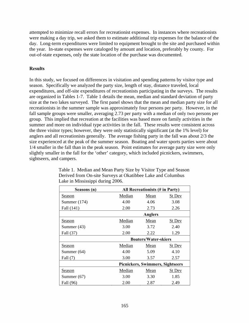
165

attempted to minimize recall errors for recreationist expenses. In instances where recreationists were making a day trip, we asked them to estimate additional trip expenses for the balance of the day. Long-term expenditures were limited to equipment brought to the site and purchased within the year. In-state expenses were cataloged by amount and location, preferably by county. For out-of-state expenses, only the state location of the purchase was documented.

Results In this study, we focused on differences in visitation and spending patterns by visitor type and season. Specifically we analyzed the party size, length of stay, distance traveled, local expenditures, and off-site expenditures of recreationists participating in the surveys. The results are organized in Tables 1-7. Table 1 details the mean, median and standard deviation of party size at the two lakes surveyed. The first panel shows that the mean and median party size for all recreationists in the summer sample was approximately four persons per party. However, in the fall sample groups were smaller, averaging 2.73 per party with a median of only two persons per group. This implied that recreation at the facilities was based more on family activities in the summer and more on individual type activities in the fall. These results were consistent across the three visitor types; however, they were only statistically significant (at the 1% level) for anglers and all recreationists generally. The average fishing party in the fall was about 2/3 the size experienced at the peak of the summer season. Boating and water sports parties were about 1/4 smaller in the fall than in the peak season. Point estimates for average party size were only slightly smaller in the fall for the ‘other’ category, which included picnickers, swimmers, sightseers, and campers.

Table 1. Median and Mean Party Size by Visitor Type and Season Derived from On-site Surveys at Okatibbee Lake and Columbus Lake in Mississippi during 2006.

Seasons (n) All Recreationists (# in Party) Season Median Mean St Dev Summer (174) 4.00 4.06 3.08 Fall (141) 2.00 2.73 2.26

Anglers Season Median Mean St Dev Summer (43) 3.00 3.72 2.40 Fall (37) 2.00 2.22 1.29

Boaters/Water-skiers Season Median Mean St Dev Summer (64) 4.00 5.09 4.10 Fall (7) 3.00 3.57 2.57

Picnickers, Swimmers, Sightseers Season Median Mean St Dev Summer (67) 3.00 3.30 1.85 Fall (96) 2.00 2.87 2.49

166

A few differences in length of stay were also evident across seasons as detailed in Table 2.1 The median visit was only one day in both periods and the average length of stay was between two and two and a half days. This difference was not statistically significant for all recreationists as a whole. According to the point estimates, the differences in average stay were most pronounced among anglers. For these visitors, the median length of stay drops by 2/3 in the fall and the average visit decreases by nearly a full day. The length of stay for boaters and water-skiers is slightly longer for those participating in the summer, but the length of stay did not differ significantly by season for those recreationists in the ‘other’ category. The main result presented in this table was that anglers and boaters tend to cut their fall visits a bit shorter than their summer visits. This was probably weather related in the case of boaters, but in the case of fishermen it may also be the result of diminishing returns. After a long fishing season, anglers may be less interested in pursuing their pastime than earlier in the season.

Table 2. Median and Mean Length of Stay by Visitor Type and Season Derived from On-site Surveys at Okatibbee Lake and Columbus Lake in Mississippi during 2006.

Seasons All Recreationists (Days) Season Median Mean St Dev Summer (170) 1.00 2.08 2.23 Fall (140) 1.00 2.39 2.34 Anglers Season Median Mean St Dev Summer (43) 3.00 3.07 2.55 Fall (37) 1.00 2.19 2.59 Boaters/Water-skiers Season Median Mean St Dev Summer (64) 1.00 1.41 1.50 Fall (6) 1.00 1.00 0.00 Picnickers, Swimmers, Sightseers Season Median Mean St Dev Summer (64) 1.00 2.10 2.39 Fall (96) 1.00 2.56 2.29

Travel times by visitor type and season were reported in Table 3. These data were computed for each visitor using Mapquest.com to calculate the travel time between the respondent’s reported county of residence and lake location. The descriptive statistics listed were only for in-state residents, which could be measured more precisely from the collected data. While not much difference occurred across seasons for recreationists as a whole, anglers and boaters and water skiers tended to travel longer distances in the summer than in the fall. The point estimates for

1 For comparison purposes we eliminated five observations from the sample which heavily skewed the results. Each of these outliers resided at the lakes for more than a month and as long as six months. Two stayed for one month, two stayed for two months, and one stayed for six months. Four of these long-term visitors were interviewed in the summer, one was interviewed in the fall.

167

picnickers, swimmers, sightseers, and campers indicated longer travel in the fall. None of these results were conclusive, however, as they were not significant at conventional levels.

Table 3. Median and Mean Travel Times by Visitor Type and Season Derived from On-site Surveys at Okatibbee Lake and Columbus Lake in Mississippi during 2006.

Seasons (n) All Recreationists (Minutes) Season Median Mean St Dev Summer (147) 24.00 40.48 38.19 Fall (126) 24.00 41.46 36.83 Anglers Season Median Mean St Dev Summer (34) 35.00 42.56 30.51 Fall (37) 51.00 55.70 43.88 Boaters/Water-skiers Season Median Mean St Dev Summer (52) 24.00 39.10 42.22 Fall (7) 24.00 48.43 34.45 Picnickers, Swimmers, Sightseers Season Median Mean St Dev Summer (61) 35.00 40.51 38.96 Fall (82) 24.00 34.44 31.67

Note: In-state visitors only Table 4 provided some additional documentation regarding recreational travel patterns across seasons. In the summer, 15.5% of visitors came from other U.S. states. While many originated in neighboring Alabama, some traveled from as far away as New Jersey and Montana. In the fall, only 10.6% of visitors come from out-of-state. The proportion of local visitors also differed seasonally. Forty-eight percent of fall visitors came from the county in which the lake was located, but only 42.5% of summer visitors were local residents. The lower incidence of out-of- state visitors and the higher the incidence of local visitors in the fall have important ramifications for gauging the economic impact of recreational facilities. Debate continues on just how much of local visitor spending should be included in economic impact models but this data suggested a higher percentage of off-season spending is not new money injected into the local economy but rather local money that is not escaping to other recreation sites or anywhere else.

While this was an interesting observation, perhaps the most important results of this research were shown in Table 5. As part of the recreational survey, respondents were asked to estimate the per person on-site and trip-related expenditures they made during their trip. Table 5 reported on the median, mean, and standard deviation for this type of spending. These numbers included such items as access fees, food, drinks, ice, lodging, souvenirs, bait, equipment rents, parking, and other expenses incurred at the site itself. They also included transportation, off-site lodging, off-site food, miscellaneous shopping, but do not include other long-term expenditures such as equipment or registration fees.

168

Table 5 indicated that overall per visitor expenditure rose in the fall compared to the summer season. However, anglers spent about $35 locally per visitor day and boaters spend about $28 per visitor day, regardless of the season. Differences were driven by picnickers, swimmers, sightseers, and other recreationists who spend about $15 more per visitor day in the fall than in the summer season. It was likely that these results were driven by the type of activity in which the recreationists were engaging. For instance, in the fall, when temperatures were cooler, more visitors were camping and less were swimming. Camping required greater expenditures than swimming but also usually entailed a lengthier stay. Our surveys reinforced the common result that day-users typically spent less than overnighters.

Table 4. Origin of Recreational Visitors by Season Derived from On-site Surveys at Okatibbee and Columbus Lake in Mississippi during 2006.

Seasons Within County Other MS Counties Other U.S. States % % %

Summer 42.5 41.9 15.5 Fall 48.2 41.1 10.6

Table 5. Median and Mean Local Expenditures by Visitor Type and Season Derived from On-site Surveys at Okatibbee Lake and Columbus Lake in Mississippi during 2006.

Seasons (n) All Recreationists ($) Season Median Mean St Dev Summer (174) 19.75 28.22 35.08 Fall (141) 24.00 37.47 38.79 Anglers Season Median Mean St Dev Summer (43) 26.00 35.17 41.80 Fall (37) 25.00 34.51 25.41 Boaters/Water-skiers Season Median Mean St Dev Summer (64) 19.75 27.67 33.34 Fall (7) 24.67 27.55 10.62 Picnickers, Swimmers, Sightseers Season Median Mean St Dev Summer (67) 13.50 24.21 31.71 Fall (96) 22.50 39.30 43.95

Table 6 detailed expenditure patterns by length of stay for both summer and fall visitors. In all cases, the point estimates indicated that per visitor day expenditure was greater in the fall than in the summer. In general, there was a larger gap between expenditures for day-users and expenditures for visitors spending a few days or more at the lake. Day users spent in the neighborhood of $22 to $27 on average, while overnighters spent in the range of $40 to $54 on

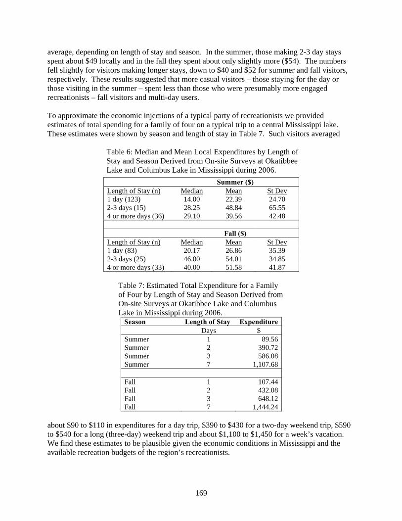
169

average, depending on length of stay and season. In the summer, those making 2-3 day stays spent about $49 locally and in the fall they spent about only slightly more ($54). The numbers fell slightly for visitors making longer stays, down to $40 and $52 for summer and fall visitors, respectively. These results suggested that more casual visitors – those staying for the day or those visiting in the summer – spent less than those who were presumably more engaged recreationists – fall visitors and multi-day users. To approximate the economic injections of a typical party of recreationists we provided estimates of total spending for a family of four on a typical trip to a central Mississippi lake. These estimates were shown by season and length of stay in Table 7. Such visitors averaged

Table 6: Median and Mean Local Expenditures by Length of Stay and Season Derived from On-site Surveys at Okatibbee Lake and Columbus Lake in Mississippi during 2006.

Summer ($) Length of Stay (n) Median Mean St Dev 1 day (123) 14.00 22.39 24.70 2-3 days (15) 28.25 48.84 65.55 4 or more days (36) 29.10 39.56 42.48 Fall ($) Length of Stay (n) Median Mean St Dev 1 day (83) 20.17 26.86 35.39 2-3 days (25) 46.00 54.01 34.85 4 or more days (33) 40.00 51.58 41.87

Table 7: Estimated Total Expenditure for a Family of Four by Length of Stay and Season Derived from On-site Surveys at Okatibbee Lake and Columbus Lake in Mississippi during 2006.

Season Length of Stay Expenditure Days $ Summer 1 89.56Summer 2 390.72Summer 3 586.08Summer 7 1,107.68 Fall 1 107.44Fall 2 432.08Fall 3 648.12Fall 7 1,444.24

about $90 to $110 in expenditures for a day trip, $390 to $430 for a two-day weekend trip, $590 to $540 for a long (three-day) weekend trip and about $1,100 to $1,450 for a week’s vacation. We find these estimates to be plausible given the economic conditions in Mississippi and the available recreation budgets of the region’s recreationists.

170

Conclusions Surface water impoundments can generate substantial quality-of-life improvements and economic impacts for rural areas. These impacts depend critically on how many recreationists frequent the lake, where they come from, how long they stay, what activities they engage in by season, and most importantly how much they spend. This study reported the results of a local recreational survey conducted at existing U.S. Army Corps of Engineers lakes in Mississippi. Our findings suggested that seasonal fluctuations occurred not only in visitor numbers, but also in length of stay, party size, distance traveled, and local expenditures. This result suggested that researchers interested in determining the economic or fiscal benefits of recreational surface water impoundments should proceed with caution when incorporating data collected in one visitor season to make yearly projections. Finally, this paper generated reasonable estimates of the per visitor economic injection that can be expected from surface water impoundments in central Mississippi Literature Cited Deller, S.C., T. Tsai, D.W. Marcouiller, D.B.K. English. 2001. The Role of Amenities and

Quality of Life in Rural Economic Growth. American Journal of Agricultural Economics, vol. 83, iss. 2, pp. 352-365.

Grado, S.C., D.L. Grebner, I.A. Munn, and R.O. Drier. 2002. Economic Feasibility Study for

Recreational Development on the Bienville National Forest in Mississippi. Final Project Report to the USDA Forest Service. Forest and Wildlife Research Center, Mississippi State University, Mississippi State, Mississippi, 110 pp.

Grado, S.C., D.L. Grebner, R.O. Drier, and I.A. Munn. 2004. Economic feasibility study for

recreational development on the Bienville National Forest in Mississippi. In Proceedings of the 2003 Southern Forest Economics Workshop. “Bugs, Budgets, Mergers, and Fire: Disturbance Economics.” New Orleans, Louisiana on March 17-18, 2003. pp. 211-220.

Rezek, J. G. Evans, S.C. Grado, and M.D. Hudson. 2006a. Choctaw County Lake

Impoundment: Economic Impact Report. Final Report to the USDA Natural Resources Conservation Service. 69 pp.

Rezek, J. G. Evans, S.C. Grado, and M.D. Hudson. 2006b. Madison County Economic

Develpoment Report.. Final Report to the Madison County Economic Development Authority, Madison County, Mississippi. 22 pp.

U.S. Department of Interior and U.S. Department of Commerce (USDI and USDC). 2002. 2001

National Survey of Fishing, Hunting, and Wildlife-Associated Recreation, Mississippi, U.S. Dept. of Interior, Fish and Wildlife Service and U.S. Dept. of Commerce, Bureau of Census. U.S. Government Printing Office, Washington, D.C., USA.

171

Factors Determining Per Acre Market Value of Hunting Leases on Sixteenth Section Lands in Mississippi*

Jacob Rhyne and Ian A. Munn1 Abstract: We examined hunting lease prices on Sixteenth Section Lands in Mississippi. Hunting leases are auctioned to the highest bidder via sealed bids with the current lessee given the right to match the highest bid. The hedonic method was used to measure the impact of cover type, average Boone and Crocket score and location on hunting lease revenue. Lands in southwest MS with a greater proportion of hardwoods and higher B&C scores generated more revenue than otherwise similar lands in the rest of Mississippi. A policy implication was that land managers may be able to increase revenue by investing in habitat improvement. Keywords: Boone and Crocket score, hedonic pricing, hunting leases, market segmentation, Sixteenth Section Lands Introduction The state of Mississippi was formed from a portion of the Mississippi Territory in 1817. While creating the boundaries for the state, Congress set aside the sixteenth section of every township in Mississippi to support public education. School Boards in Mississippi control all such set aside lands within their school district. Sixteenth Section Lands generate income for education through the sale of timber and from various leases such as oil, gas, mineral, and hunting. Hunting leases on Sixteenth Section Lands are awarded to the highest bidder in a sealed bid auction. The hunting leases are usually advertised in local newspapers. Interested parties respond by bidding on the lease. The highest bidder is awarded the lease with the current lessee given the option of retaining the lease by matching the highest bid. Hunting leases on Sixteenth Section Lands generated more than 2.5 million dollars in revenue in 2005. Approximately 300,000 acres of Sixteenth Section Lands in Mississippi were leased for hunting. Many factors affect hunter willingness to pay for hunting rights on a particular location. Factors such as game quality, habitat quality and location have proven to impact hunting lease prices (Livengood 1983, Loomis et al. 1989, Stribling 1992). The objective of this study was to determine the impact of these factors on hunting lease prices for Sixteenth Section Lands in Mississippi. Hunting leases are made up of a collection of inseparable attributes such as habitat quality, game quality and location. The underlying hypothesis of this study was that each of these attributes influences the amount of revenue that a hunting lease generated. Understanding how these factors influence hunting lease prices on Sixteenth Section Lands will provide School

* This manuscript is FO-0352 of the Forest and Wildlife Research Center, Mississippi State University. 1 Graduate Student and Professor, respectively, Forestry Department, Forest and Wildlife Research Center, Mississippi State University, dr312@msstate.edu (J. Rhyne), imunn@CFR.MsState.Edu (I. Munn), (662) 325-4546 (v).

172

Boards with base line information to evaluate the performance of their lease program relative to the rest of the state and suggest ways to improve lease revenues in the future. Methods and Data

The hedonic method (Rosen 1974) was used to decompose the lease price, and determine the contribution of habitat quality, game quality, and market segmentation to lease price. The method has been used by others to determine the impact of individual lease characteristics on lease prices (Zhang et al. 2006, Munn et al. 2005). Accordingly, the hedonic price equation was specified as: Lease price per acre = F [habitat quality, game quality, location] The dependent variable was the gross lease revenue per acre expressed in logarithmic form (log revenue). Habitat quality was represented by the percentage of the leased area in various forest cover types such as pines, hardwoods, mixed pine-hardwoods, open lands, recently regenerated lands, and water. Game quality was approximated by an average Boone and Crocket score for bucks in the county. Market segments were delineated into three broad regions based on the major population centers in the state. The resulting market segments were southwest Mississippi, northwest Mississippi, and east Mississippi. As hedonic pricing theory does not dictate which functional form to use, we experimented with several options. The semi-logarithmic form best fit the data. Hunting leases that contained 600 or more acres were selected for analysis. This restriction was imposed because cover type information was provided for the entire section although leases could cover all or part of a section. Selecting hunting leases with at least 600 acres leased allowed us to appropriately match the cover type information that applied to a particular lease. A total of 169 hunting leases were included. Lease price and number of acres leased. Hunting lease information was provided by the Public Lands Division of the Mississippi Secretary of State’s Office. For each hunting lease, collected information included; the number of acres leased and the amount of revenue generated. Cover type. Cover type information was provided by the Mississippi Institute of Forest Inventory (MIFI). The information included the number of acres in the following cover types for each sixteenth section: pine, hardwoods, mix pine-hardwoods, water, regenerated, and open. Acreages by cover type were converted to percentage of the total sections. Percent hardwood was the base (omitted) category in the regression analysis. Average Boone and Crocket Scores. County average Boone and Crocket scores were derived from an antler index that approximates the projected average Boone and Crocket Score for each county (Strickland and Demarais 2000). The index is derived from deer harvest data collected by the Mississippi Department of Wildlife Fisheries and Parks through the Deer Management Assistance Program (DMAP). DMAP monitors the deer population in Mississippi by taking biological samples from harvested game on wildlife management areas and from participating landowners. Data includes antler measurements and deer weight.

173

Geographic Regions of the state. The state was divided into three regions to determine the impact of market segmentation on hunting lease revenue. The three geographic regions selected were east Mississippi, southwest Mississippi, and northwest Mississippi. The northwest and southwest regions include the Mississippi Delta which is a highly demanded hunting area. To model market segmentation, three dummy variables were introduced to differentiate between regions. For instance, the dummy variable for northwest MS =1 for hunting leases in this region, else 0. Dummy variables for other regions were similarly constructed. The dummy for the east region served as the base category in estimation. Results

Descriptive statistics. The average annual lease price was $5,041.37 or $7.93 per acre. Pine stands constituted 45% of the leased area, hardwoods 28%, mixed pine-hardwoods 13%, regenerated forests 8%, and open land and water accounted for the residual. The average projected average Boone and Crocket Score by county was 110. Table 1. Descriptive statistics related to hunting leases on Sixteenth Section Lands in Mississippi in 2005 (N=169) Variables Mean Std Dev. Annual lease price ($) 5,041.37 4,248.03 Annual lease price/acre ($) 7.93 6.61 Log lease price/acre 1.83 0.66 Avg. tract size (acres) 636.98 17.10 Log-acres leased 6.46 0.03 Southwest Mississippi 0.40 0.49 Northwest Mississippi 0.11 0.31 East Mississippi 0.49 0.50 % Pine 45.03 29.10 % Mixed pine-hardwoods 13.01 8.50 % Water 0.33 1.25 % Water squared 1.67 10.82 % Regeneration 7.85 10.51 % Open 5.27 9.54 % Hardwoods 28.51 28.16 Avg. Boone & Crocket Score 110.31 13.69 Regression results. Of ten coefficients included in the model, six were significant (Table 2). Our estimation results corroborate with findings by others (Stribling et al. 1992). For instance, of the set of variables representing habitat quality, percent pine and regenerated lands were associated with significantly negative coefficients. This suggested that pine cover types and recently regenerated lands reduced lease revenue. A one percent increase in the percent share of land with pines and regenerated areas caused lease price to decrease by 0.338 % and 0.068 %,

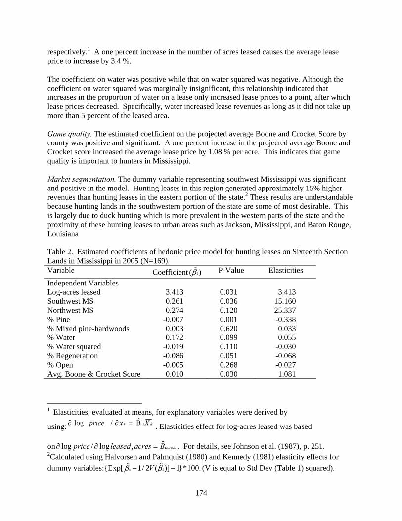
174

respectively.1 A one percent increase in the number of acres leased causes the average lease price to increase by 3.4 %. The coefficient on water was positive while that on water squared was negative. Although the coefficient on water squared was marginally insignificant, this relationship indicated that increases in the proportion of water on a lease only increased lease prices to a point, after which lease prices decreased. Specifically, water increased lease revenues as long as it did not take up more than 5 percent of the leased area. Game quality. The estimated coefficient on the projected average Boone and Crocket Score by county was positive and significant. A one percent increase in the projected average Boone and Crocket score increased the average lease price by 1.08 % per acre. This indicates that game quality is important to hunters in Mississippi. Market segmentation. The dummy variable representing southwest Mississippi was significant and positive in the model. Hunting leases in this region generated approximately 15% higher revenues than hunting leases in the eastern portion of the state.2 These results are understandable because hunting lands in the southwestern portion of the state are some of most desirable. This is largely due to duck hunting which is more prevalent in the western parts of the state and the proximity of these hunting leases to urban areas such as Jackson, Mississippi, and Baton Rouge, Louisiana Table 2. Estimated coefficients of hedonic price model for hunting leases on Sixteenth Section Lands in Mississippi in 2005 (N=169). Variable Coefficient )ˆ( kβ P-Value Elasticities Independent Variables Log-acres leased 3.413 0.031 3.413 Southwest MS 0.261 0.036 15.160 Northwest MS 0.274 0.120 25.337 % Pine -0.007 0.001 -0.338 % Mixed pine-hardwoods 0.003 0.620 0.033 % Water 0.172 0.099 0.055 % Water squared -0.019 0.110 -0.030 % Regeneration -0.086 0.051 -0.068 % Open -0.005 0.268 -0.027 Avg. Boone & Crocket Score 0.010 0.030 1.081

1 Elasticities, evaluated at means, for explanatory variables were derived by

using: kXxprice kk Β=∂∂ ˆ/log . Elasticities effect for log-acres leased was based

on .ˆ,log/log acresBacresleasedprice =∂∂ . For details, see Johnson et al. (1987), p. 251. 2Calculated using Halvorsen and Palmquist (1980) and Kennedy (1981) elasticity effects for dummy variables:{Exp[ .100*}1)]ˆ(2/1ˆ −− kk V ββ (V is equal to Std Dev (Table 1) squared).

175

Summary

This study used the hedonic price method to determine how habitat quality, game quality and location impacted hunting lease prices on Sixteenth Section Lands in Mississippi. All three variables significantly influenced hunting lease prices. Our findings that pine and regenerated areas did not generate as much lease revenue as hardwoods is consistent with results found by Stribling et al. (1992) in Alabama. Hunters perceive that pine and regenerated areas do not provide as high quality habitat for game as leases that contain plentiful hardwoods. Therefore, hunters are not willing to pay as much for a hunting lease that contains pine and regenerated areas as they would for a comparable hunting lease in size and location in hardwoods. The results of this study agreed with findings of other researchers that showed that hunting leases with a year round water supply generate greater revenue (Munn et al. 2005 and Zhang et al. 2006). However, this study also found that too much water at a particular location causes the lease price to decrease. Having a water source improves habitat for game but wetland areas can impede access and make removal of harvested game difficult (Harper et al. n.d.). Our findings agreed with results by other studies (Standiford and Howitt 1993, Pope and Stoll 1985, and Messonnier and Luzar 1990) that there is a positive relationship between lease revenue per acre and average lease size. Other studies, however, have found a negative relationship (Shrestha and Janaki 2004). Our study found that hunters are willing to pay more money to have the opportunity to hunt better quality game in Mississippi. This result corroborated findings by Loomis and Fitzhugh (1989) and Standiford and Howitt (1993). Uncommon quality game is prized by hunters. Lease revenue varied across regions of the state. Hunting leases in the southwestern region were significantly greater than hunting leases in the eastern region. This shows that there are different hunting markets in Mississippi which must be accounted for in modeling lease markets. This is very similar to the results that Pope and Stoll (1985) who examined the impact of market segmentation on hunting leases in Texas. It is important that future studies using the hedonic method to examine hunting lease prices consider the impact of market segmentation. Different hunting markets could be attributed to supply and demand of hunting areas in state. For example, hunting leases in the southwestern region are very desirable and command a premium largely due to the duck hunting that occurs in the Delta. Areas for duck hunting are not nearly as plentiful in the eastern region. The results also suggest that hunters in different regions of the state do not purchase hunting leases in other regions. It might be that because hunters prefer a hunting location near their home. Having a hunting lease located nearby, allows the hunter to take more hunting trips and decreases the time and cost associated with hunting.

176

Discussion Based on these findings, School Boards can improve hunting lease revenues in several ways. First, improving wildlife habitat by planting mast-producing trees in pine stands and refraining from harvesting all mast-producing trees on regenerated areas can increase hunting revenue. Second, water on the property also increases lease revenue suggesting that creating water bodies (e.g. ponds, water impoundment levees, etc.) on leased areas that do not have a natural water source may be a viable practice. Third, in light of the fact that larger leases generated more per acre revenue, School Boards should consider bundling larger blocks together, instead of breaking sections up into multiple leases. This study did not examine the costs of making these changes; however, assistance is available from Federal Agencies and NGOs. The costs of these changes are worth considering because Sixteenth Section Lands will be owned by the schools in Mississippi for the foreseeable future. This will provide a long horizon in which to recoup costs incurred from providing better habitat. Each School Board must decide if these suggested changes would be worthwhile. The model also provides School Boards with an estimate of how much revenue their hunting leases should generate based upon the characteristics of those leases. If a lease does not generate as much revenue as other leases with comparable characteristics, a possible solution might be a more intensive marketing strategy for the lease. Literature Cited

Halvorsen, R., and R. Palmquist. 1980. The interpretation of dummy variables in semi-

logarithmic equations. Am. Econ. Rev. 70(3):474-475. Harper, A.C., E.C. Dixon, M.P. Jakus, and D.A. Barefield. n.d. Earning additional income

through hunt leases on private land. The Agricultural Extension Service. The University of Tennessee, PB1627.

Johnson, A.A., M.B. Johnson, and R.C. Buse. 1987. Econometrics:basic and applied.

Macmillan Publishing, Inc. New York USA. Kennedy, E.P. 1981. Estimation with correctly interpreted dummy variables in semi-logarithmic

equations. Am. Econ. Rev. 71(4):801. Livengood, K.R. 1983. Value of big game form markets for hunting leases: the hedonic

approach. Land Econ. 59(3):287-291. Loomis, J.B., and L. Fitzhugh. 1989. Financial returns to California landowners for providing

hunting access: Analysis and determinants of returns and implications to wildlife management. Trans N. Am. Wildl. Natur. Resourc. Conf: 197-201.

Messonnier, M.L., and E.J. Luzar. 1990. A hedonic analysis of private hunting land attributes

using an alternative functional form. South. J. Agric. Econ. 22(2):129-135.

177

Munn, I.A, E.K. Loden, S.C. Grado, J.C. Jones, and W.D. Jones. 2005. Comparing hunting lease prices: A price decomposition approach. P. 193-200 in: Proceedings of the 2004 Annual Southern Forest Economics Workshop. Alavalapati, R.R. and D.R. Carter, eds. March 14-16, 2004. St. Augustine, FL.

Pope, C.A., and J.R. Stoll. 1985. The market value of ingress rights for white-tailed deer hunting

in Texas. South. J. Agric. Econ. 17(1):177-182 Rosen, S. 1974. Hedonic prices and implicit markets: Product differentiation in pure

competition. J. Polit. Economy 82:34-555. Shrestha, R.K., and R.A. Janaki. 2004. Effect of ranchland attributes on recreational hunting in

Florida: A hedonic price analysis. J. Agric. Appl. Econ. 36(3):763-772. Standiford R.B., and R.E. Howitt. 1993. Multiple use management of California’s hard-wood

rangelands. Journal of Range Management 46(2):176-182. Stribling, H.L., J.P. Caulfied, B.G. Lockaby, D.P. Thompson, H.E. Quicke, and H.A. Clonts.

1992. Factors influencing willingness to pay for deer hunting in the Alabama piedmont. South. J. Appl. For. 16(3):125-129.

Strickland, B.K., and S. Demarais. 2000. Age and regional differences in antlers and mass of

white-tailed deer. J. Widl. Manage 64:903-911. Zhang, D., A. Hussain, and J.B. Armstrong. 2006. Supply of hunting leases from non-industrial

private forest lands in Alabama. Human Dimensions of Wildlife 11:1-14.

178

Influence of Field Windbreaks on Landscape Aesthetics: Preliminary Results

Robert K. Grala1, John C. Tyndall2, and Carl W. Mize2 Abstract: Field windbreaks provide numerous benefits such decreased soil erosion, crop and livestock protection, wildlife habitat, and carbon sequestration. They also have a significant impact on visual appearance of surrounding agricultural landscapes. Although this benefit seems to be apparent, little is known about what people think of field windbreaks and which windbreak features are the most important for aesthetic reasons. A mail survey was conducted to reveal opinions of Iowa residents on field windbreaks and their influence on visual appearance of agricultural landscapes. Additionally, respondents’ willingness to support financially windbreak programs was examined. The survey was sent to 3,500 respondents including 1,500 farm operators and 2,000 non-farmers. The overall response rate was 40%. A telephone follow-up was conducted to test for non-response bias; responses from 155 non-respondents were obtained. It seems that aesthetic benefits of field windbreaks were widely recognized by respondents. About 74% of them indicated that field windbreaks are important in diversifying agricultural landscapes, whereas 67% said that field windbreaks make agricultural landscapes visually more appealing. Further, 34% of respondents were willing to support financially a fund what would promote windbreak planting for aesthetic purposes. Keywords: Aesthetics, field windbreaks, mail survey, willingness to pay

1 Department of Forestry, Mississippi State University, Box 9681, Mississippi State, MS 39762-9681, rgrala@CFR.MsState.Edu (R. Grala), (662) 325-7039 (v). 2 Department of Natural Resource Ecology and Management, Iowa State University.

179

Willingness-to-pay Assessment of Visitors to an Off-highway Vehicle Recreation Area: An Individual Travel Cost Method Approach

Gregory Parent1, Janaki Alavalapati1, Taylor Stein1, and Chris Reed2 Abstract: To date the little research that has been done on off-highway vehicle recreation has largely focused on the environment / social impact of OHV recreation. This study uses the individual travel cost method to evaluate the value of OHV recreation at the Croom Motorcycle Area (CMA) in central Florida. Through on-site questionnaires and mail-back surveys researchers collected information from participants on trip expenditure, trip characteristics, and socio-demographics. Results suggest that participants with more experience in OHV recreation are more frequently visiting the site, reflecting the effect of habit formation. Regression coefficients were used to estimate consumer surplus associated with OHV recreation at CMA. The total annual willingness to pay (WTP) of all households recreating at the CMA was evaluated at over $39 million. Results of this research help Florida Division of Forestry in making planning and management decisions relating to OHV recreation in Florida. Keywords: Resource valuation, off-highway vehicle recreation, willingness-to-pay, individual travel cost method, revealed preferences

1 School of Forest Resources and Conservation, Institute of Food and Agricultural Sciences, University of Florida, PO Box 110410, Newins-Ziegler Hall, Gainesville, FL 32611, gparent@ufl.edu (G. Parent), (603)767-3669 (v). 2 Florida Division Forestry.

180

Role of Natural Amenity Resources in Retiree Location Choice Behavior: Potential Concern for Economic Growth and Ecological Disturbance in Rural America

Neelam C. Poudyal1, Donald G. Hodges2, and Ken Cordell3 Abstract: Most local governments have traditional strategies for economic development such as raising the tax rate, attracting industries, and promoting heavy-duty manufacturers that can have detrimental impacts on environment and quality of life. Even in the rural areas, many of the farming and mining dependent counties experienced a decline in business in recent decades. Recently, retirees have been identified as an economic force that can have significant multiplier effects on local economies. Those include restructuring the local economy, generating higher tax revenue, increasing expenditure and money flow, creating more jobs, donating and providing voluntary supports, and often paying for other public goods that raise the quality of life in the area. This paper examines the relationship between the nature-based outdoor resources (land, water and environment based) amenities and retirees’ choice of their resident counties. Specifically, this paper estimates a two-stage probit model using national level data of retirees and nature-based amenity resources and then calculates the probability of each county being a retiree destination in relation to several natural amenity resources. We found that the land use diversity and scenic landscape resources are the major amenities in which retirees place great deal of value. Moreover, the proportion of public forest for outdoor recreation in the county is one of the strong factors that attract retirees to some counties. The results also reveal that lower housing cost counties in the southern and western US, with more sunny hours and warmer temperatures and abundant public forest, scenic range, or pasturelands are factors that predict the county’s probability of being developed as a retiree economy. Similarly, transportation access, miles of scenic rivers, and bigger lake amenities have positive effects on attracting retirees. Conversely, high population density, intensive agriculture, and steep topography were negatively related to retirees’ choice of location. This can be explained by the negative externality they induce by competing for open space, scenic quality, and transportation easiness. The findings from this study have several policy implications to local government officials, regional planners, and policy makers to adopt appropriate policy and design comprehensive plan to attract retirees. This will eventually be helpful to foster rural economic development of natural amenity rich counties, where other resources are issues of concern. On the other hand, the tremendous pressure on the outdoor resources with increasing retiree is likely to alter the natural landscape significantly which can have irreversible impact on environment. In addition, the findings will also be useful to conservation planners and resource managers to manage future demand for outdoor recreation and its environmental impacts in counties where retiree’s concentration is likely.

1 Department of Forestry, Fisheries and Wildlife Sciences; The University of Tennessee; Knoxville, TN 37996, npoudyal@utk.edu. 2 Department of Forestry, Wildlife and Fisheries; The University of Tennessee; 274 Ellington Plant Sciences Bldg.; Knoxville, TN 37996-4563; dhodges2@utk.edu; (865) 974-2706 (v). 3 Forestry Sciences Laboratory, USDA Forest Service, Athens, Georgia 30602.

181

Nonmarket Valuation Based on Market Information: An Application to U.S. Forest Resources

Jianhua Cao1 and Daowei Zhang2 Abstract: Forest is a complex ecosystem which can provide a array of ecosystem services. This paper focuses on valuing forest resource as ecological resources. It reviews the literatures on market valuation and nonmarket valuation and presents a new analytical framework for valuing forest ecological resources. Using the new framework, the value of forest ecosystem services is estimated at $171.5 billion/year, which is 149% of the value adds in the forest industries or 1.64% of GDP of the U.S., respectively. Keywords: Forest resources, ecosystem services, nonmarket valuation

1 Visiting Scholar, School of Forestry and Wildlife Sciences, Auburn University, AL 36849-5418. 2 Professor, School of Forestry and Wildlife Sciences, Auburn University, AL 36849-5418, zhangdw@auburn.edu, (334)-844-1067 (v), (334)-844-1084 (fax).

182

Factors Driving Deforestation in Common-Pool Resources in Durango, Mexico

Gustavo Perez-Verdin1, Yeon-Su Kim2, Denver Hospodarsky2, and Aregai Tecle2

Abstract: The theory of collective action has been extensively used to evaluate the relationship between common-based property regimes and the conservation of natural resources. However, there are two key components of the theory that literature reports as puzzles in which no consensus exists about their effect on the performance of common pool resources. Those are group size and heterogeneity. This study analyzes the effects of these two components on the effectiveness of community-based forestry, called ejidos, to protect their forest resources in Durango, Mexico. Sixteen explanatory variables attempt to evaluate the two puzzles and the success of ejidos, the dependent variable, defined by the absence/presence of deforested, degraded, or forested conditions. We used a multinomial logit model to determine the contribution of each explanatory variable and the importance of the two puzzles. The results show that corn yield, level of marginality, percent of forest area, total population, a forest value index, distance to markets, roads and towns, were all statistically significant in determining deforested conditions. Deforestation becomes more attractive for poor communities and as corn yield and distance to towns, roads, and markets decrease. In general, group size and heterogeneity had no significant effects on the presence of deforested conditions. We argue, however, that current institutional policies should shift their focus to reduce the marginality problem in poor communities which will eventually reduce the rate of local deforestation. Keywords: Ejido, deforestation, collective action, random utility model, multinomial logit model, Durango, Mexico

1 Mississippi State University, Department of Forestry. Box 9681. Mississippi State, MS, 39762, gperez@cfr.msstate.edu, (662) 325-6822 (v). 2 Northern Arizona University, School of Forestry. Box 5018. Flagstaff, AZ. 86011.

183

Determinants of Forest Preservation

J.A. Anderson1, 2, M.K. Luckert2, and W.L. Adamowicz2

Abstract

Between 1992 and 2003, the global area under preservation has increased 52.8%, such that the terrestrial proportion of the globe now protected is 11.5% (Chape et al. 2003). Since some countries protect more forest than others, we wish to explain this variation using a reduced-form model capable of suggesting whether the amount of forest a country preserves is related to economic and ecological factors. More specifically, this paper will investigate whether there appears to be a relationship between forest preservation and forest intensification, since this would suggest that some countries are using intensive zones to offset timber losses from forest preservation. There is a robust literature exploring systematic approaches for efficiently selecting forest reserves (e.g., Ando et al. 1998, Polasky et al. 2005, etc.), but we could find no multi-country empirical studies that estimate whether plantation forestry appears to be a technique by which countries are increasing forest preservation. If such a relationship between plantations and preservation were found, then policy alternatives for promoting plantation forestry, as will be suggested in this paper, could be used to promote preservation. Although reduced-form models, as will be used in this paper, are not always supported by theoretical underpinnings, they can still quantify direct and indirect aggregate effects of variables on forest preservation (Grafton et al. 2004). This methodology is supported by the reduced-form modeling used in: (i) multi-country analyses that correlate explanatory factors with deforestation, (ii) empirical work done on detailing the environmental Kuznets curve (EKC), and (iii) analyses of the impact of trade on the environment. In general, these three branches of the literature test whether environmental degradation is related to factors such as income, time, trade, and sometimes other variables, such as population density and polity. The literature on deforestation, the EKC, and trade-environment linkages also provide insights into the economics of forest preservation. The deforestation literature suggests that forest conversion is an important factor in fueling the economic growth of developing countries (Naidoo 2004). This result agrees with the “classic” finding of the EKC literature, that environmental quality initially decreases with rising per-capita income. But the EKC literature has more to add: suggesting that, in some cases, as income rises, environmental degradation eventually reaches a turning point, after which environmental quality begins to rise (Grafton et al. 2004). This second EKC finding—that economic growth might eventually benefit the environment—is also found in the trade and environment literature for some forms of environmental quality and for some regions. This relationship can arise when there are income, technique or composition effects that result in improved environmental quality and increased income (Copeland and Taylor 2004). Therefore it is possible that trade, which promotes economic growth, may have a beneficial effect on some measures of environmental quality 1 Corresponding author, jaya@ualberta.ca. 2 Department of Rural Economy, 515 GSB, University of Alberta, Edmonton, AB, Canada, T6G 2H1.

184

(Frankel and Rose 2005). Finally, applying these general results to our forestry question, we examine the hypothesis that the increased productivity from plantation forestry could not only increase income and trade, but could also increase environmental quality by encouraging forest preservation—i.e., a positive technique effect. Empirically testing this hypothesis (of a positive technique effect) will be the main objective of this paper. Since this technique effect could arise via an EKC with respect to forest preservation, we will also test for the presence of such an EKC. The econometrics will incorporate the following multi-country data for the year 2000: (i) hectares of preserved forest, (ii) ratio of forestry value-added to GDP, (iii) total hectares of land, (iv) per capita income, (v) polity, (vi) forestry imports, (vii) ratio of forestry exports and imports to total forestry value-added, (viii) proportion of forest that is publicly owned, and (ix) hectares managed as forest plantations. Literature Cited Ando, A., J. Camm, S. Polasky, and A. Solow. 1998. Species distributions, land values, and

efficient conservation. Science 279 (5359): 2126-2128. Chape, S., S. Blyth, L. Fish, P. Fox, and M. Spalding (compilers). 2003. “2003 United Nations

list of protected areas.” IUCN, Gland, Switzerland and Cambridge, UK and UNEP-WCMC, Cambridge, UK. Ix + 44pp.

Copeland, B.R. and M.S. Taylor. 2004. Trade, Growth and the Environment. Journal of

Economic Literature. XLII (March): 7-71. Frankel. J.A. and A.K. Rose. 2005. Is trade good or bad for the environment? Sorting out the

causality. The Review of Economics and Statistics 87(1):85-91. Grafton, R.Q., W. Adamowicz, D. Dupont, H. Nelson, R.J. Hill, and S. Renzetti. 2004. “The

economics of the environment and natural resources.” Blackwell Publishing, Malden, MA. pp.503.

Naidoo, R. 2004. Economic growth and liquidation of natural capital: the case of forest

clearance. Land Economics 80(2): 194-208. Polasky, S., E. Nelson, E. Lonsdorf, P. Fackler, and A. Starfield. 2005. Conserving species in a

working landscape: land use with biological and economic-objectives. Ecological Applications 15 (6): 2209-2209.

185

A Marginal Cost Analysis of Trade-offs in Preservation of Old Growth in an Even Aged Boreal Forest of Ontario

Rajender P.Khajuria1 and Susanna Laaksonen-Craig2

Abstract: Marginal cost (MC) curves are developed for preservation of old growth in an even aged forest in north east Ontario. MC of preservation of old growth, when forest managers are faced with the task of achieving multiple objectives under sustainable forest management (SFM) is investigated. The implications of considering SFM objectives of providing regular supply of timber per period, ensuring that terminal volume at the end of planning horizon meets a given target and maintaining a desired age structure of the forest, are studied and MCs derived. Trade-offs in preservation of old growth are derived, when the levels of these equally important objectives of SFM are allowed to vary. We observed that MCs are more varied for these three scenarios when area allotted for old growth preservation is small. When old growth forest protected reaches about 66% of the maximum possible, the MCs are almost similar. Even flow volume per period had the highest MC amongst all the three cases. MC equations of old growth for the three objectives are best estimated through semi-log regression. The MCs of old growth at different levels of these objectives are iso-elastic. Elasticity of MC of old growth when volume flow per period varies 20% is the highest whereas it is lowest for the case when volume flow per period varies by 5% only.

1 Corresponding author, Ph.D. Candidate, University of Toronto, Faculty of Forestry, 33 Willcocks St., Toronto, ON M5S 3B3, Canada, raj.khajuria@utoronto.ca, (416) 925-9181(v), (416) 978-3834 (fax). 2 Assistant Professor, University of Toronto, Faculty of Forestry, 33 Willcocks St, Toronto, ON M5S 3B3, Canada, susanna.laaksonen.craig@utoronto.ca.

186

Globalization, Market Economy and Tropical Deforestation: Evidence from Southwest China

Youxin Ma1, Yaoqi Zhang2, Hongmei Li1, Wenjun Liu 1, and Min Cao1 Abstract: Globalization and market economy play a large role in the dilemma of tropical forest conservation. On the one hand, globalization and market economy can reduce poverty and extensive cultivation on tropical forest land; on the other hand, they promote the logging and market-oriented agriculture largely influenced by the international market and capital flow. The dilemma can be seen clearly from different periods of development in SW China. In recent 2 decades globalization and free market economy have brought about profound changes in China, including the tropical area. This paper is to provide some evidence how globalization and market economy have played in the tropical deforestation in the Southwest China. As the demands of natural rubber grows and price increases on the world market, the profitability of rubber plantation on tropical rain forests increase dramatically, especially in tropical Asia where labor cost is comparatively low and market economy is emerging. In this study, we quantified land-use/land-cover change across Xishuangbanna using Landsat images from 1976, 1988, and 2003. It is obvious that rubber plantations have expanded into previous rain forest land. In 1976, forests covered approximately 70% of Xishuangbanna, but by 2003 they covered less than 50%. Tropical seasonal rain forest was the forest type most affect by the expansion of rubber plantations, and a total of 139,576 ha was lost. This deforestation results in a rapid increase of forest patch numbers and decrease of patch sizes. Keywords: Deforestation, rubber plantations, economic development, fragmentation, biodiversity conservation, land use and land cover change, Xishuagbanna

1 Xishuangbanna Tropical Botanical Garden, Chinese Academy of Sciences, 88 Xuefu Road, Kunming 650223, PR China. 2 School of Forestry and Wildlife Sciences, Auburn University, Auburn, AL 36830.

187

Performance Bonding and Reforestation of Surface Mined Lands

Jay Sullivan and Greg Amacher1 Abstract: The Surface Mining Control and Reclamation Act of 1977 (SMCRA) mandates that surface mined land in the United States be returned to a condition capable of supporting its pre-mined use or a use of higher value, and that the land be reclaimed in a fashion that renders it at least as productive after mining as it was before mining. Mine-land reclamation under SMCRA follows a process where mine operators agree to a post-mining land use and then post performance bonds held by regulators until reclamation is evaluated and deemed to be successful. A bonding process and law such as this is quite common in several other countries, such as Canada and Australia. Since 1977, the majority of mined land in the Appalachian coal region has been reclaimed as hayland/pasture. Forests on these sites would be of much higher social value given their rent-generating productive role, but also their role in increasing land values or reducing risks such as erosion, flooding, and fire that can threaten communities. Given that mine operators, who are responsible under the law for reclamation efforts, are not likely to make decisions with future land rents in mind, an externality exists in the reclamation process that undermines the intention of the law. Our purpose is to examine the social costs of mine-land reclamation, and to examine the role of several types of bond policy programs in reducing these social costs. An important part of the analysis will be to compare the socially best bond instruments with the ones used in practice. We describe both the theory of performance bonding and simulations that are based on growth functions developed on mined sites. We characterize the reclamation decisions faced by a mine operator and a benevolent social planner, we examine the role of bond payments in reducing the social costs associated with a difference in incentives between the mine operator and the social planner, we present a simulation to reveal the magnitude of social costs under various assumptions about the bond, and we examine potential inefficiencies in bond instruments the way they are currently used in practice.

1 Professors, Department of Forestry, College of Natural Resources, Virginia Polytechnic and State University, Blacksburg, VA 24061, jsulliv@vt.edu (J. Sullivan), 540-231-4356 (v), 540-231-3698 (fax).

188

Evaluation of Cogongrass Control Techniques for Nonindustrial Private Landowners in Mississippi*

Jon D. Prevost1, Donald L. Grebner2, Jeanne C. Jones2, Stephen C. Grado2, Keith L. Belli2, and John D. Byrd3

Abstract: Introduced in the winter of 1911-1912, cogongrass (Imperata cylindrica (L.) Beauv.) has invaded thousands of forested acres across the Southeast United States resulting in considerable negative impacts on forest regeneration and growth. Cogongrass grows in dense, monotypic stands which out-compete native vegetation thus decreasing biodiversity of flora and fauna. To successfully regenerate an infested pine stand, a “window” of reduced cogongrass competition must be provided. Control of this noxious grass can be obtained through the use of herbicides such as Arsenal AC and Accord Concentrate. Although long-term control is difficult to achieve, short-term control for the purpose of stand regeneration can be obtained through different combinations and levels of herbicides and surfactant. A hypothetical regeneration scenario was created to evaluate six herbicide combinations using Land Expectation Value as criteria to determine which combination is more efficient in terms of cost and cogongrass control. The herbicide combination of 3 oz/ac Arsenal AC, 15 oz/ac Accord Concentrate, 12 oz/ac SurfPro surfactant directly applied by wand at 35 gallons per acre provided an optimal combination of cost efficacy and cogongrass control. Keywords: Cogongrass, forest land, herbicides, invasive species, land expectation value, monetary returns, pine Introduction Introduced from Asia in the winter of 1911-1912, cogongrass (Imperata cylindrica (L.) Beauv) has invaded the southeastern United States resulting in substantial biological and monetary losses to forest landowners. Cogongrass was accidentally introduced into Grand Bay, Alabama as packing material for a crate of Satsuma oranges. Shortly afterwards, it was planted at experiment stations in Mississippi, Alabama, and Florida to test its potential for use as a forage crop (Tabor 1949, Tabor 1952). From these points of original infestation, cogongrass has spread by seed, rhizome, and intentional planting to cover thousands of acres across the Southeast. Cogongrass seed heads contain up to 3,000 wind disseminated inflorescences that have an average travel distance of 49 feet, but have been reported to travel over a much longer range (Holm et al. 1977). Seeds require bare soil for germination, and disturbances within a forest

* Approved for publication as journal article no. FO344 of the Forest and Wildlife Research Center, Mississippi State University. 1 Graduate Research Assistant, Box 9681 Mississippi State, MS 39762, jdp89@msstate.edu, 662-325-5812 (v). 2 Respectively, Associate Professor, Associate Professor, Professor, and Professor, Professor, Forest and Wildlife Research Center, Box 9681, Mississippi State, MS 39762. 3 Professor, Plant and Soil Sciences, Box 9555, Mississippi State, MS 39762.

189

stand such as thinning or site preparation can facilitate the establishment of this noxious weed (Shilling et al. 1997). Rhizomes, or cogongrass roots, can reach levels of 16 tons per acre and comprise up to 60% of the total biomass of a cogongrass patch (Terry et al. 1997). High rhizome densities allow cogongrass to rapidly spread and dominate across a site. Rhizomes can be spread by contaminated fill material, tires, grapples, and blades of machinery used in or around cogongrass patches (Willard 1988, Dozier et al. 1998). All that is required for establishment is 0.0035 ounces of rhizome and one rhizome can spread to cover 172 square feet in 11 weeks (Soerjani and Soemartwoto 1969, Eussen 1980). Although thriving under full sunlight, cogongrass can survive under canopy while receiving 1% ambient light (Gaffney 1996). Once established, cogongrass forms very dense, tall, monotypic stands that exclude most native vegetation other than large trees and dense shrubs resulting in lower quality wildlife habitat and an altered fire regime that can potentially damage larger pine trees (Lippincott 1997). These characteristics allow cogongrass to dominate the understory reducing biodiversity and making pine stand regeneration extremely difficult. Natural pine seedling recruitment is hampered due to the high foliar density of cogongrass which out-competes seedlings for light, water, and nutrients (Lippincott 1997). Clearcut pine sites also increase the competitive advantage of cogongrass. Increased sunlight and disturbed soil create ideal conditions for cogongrass to grow and spread (Dickens and Moore 1974). To successfully regenerate a pine stand, a “window” of control must be provided to allow for the establishment and early growth of planted or natural pine seedlings. Numerous studies have reported imazapyr and glyphosate based herbicides to be most effective in controlling cogongrass (Gaffney 1996, Willard et al. 1997, Dozier et al. 1998, Miller 2000). However, unknown are the monetary effects of controlling cogongrass for stand establishment in terms of after tax Land Expectation Value (LEV) for a pine forest management regime typical of the southeastern United States. The study objective was to analyze, compare, and discuss monetary and biological returns for alternative cogongrass control treatments and costs of site rehabilitation or planting. Methods Four cogongrass control treatments (Table 1) were compared as part of a hypothetical southern pine forest management regime using LEV as determinate criteria assuming a 6% interest rate. Treatments varied in level of Arsenal AC, Accord Concentrate, surfactant, and applied volume in gallons per acre (GPA). Treatments 1 and 2 were evaluated from 2004-2006 at the John C. Stennis Space Center in Hancock County, Mississippi. Data for treatments 3 and 4 were derived from a study done by Ramsey et al. (2003) in 1999-2001. PTAEDA3 was used to predict thin and harvest yields for a loblolly pine (Pinus taeda) plantation planted on a cogongrass infested cutover site. Four treatments were considered in conjunction with mechanical site preparation in year zero to provide a “window” of reduced cogongrass competition to allow for successful regeneration. Revenues included $651.21 from thinning at age 17, and $5,248.18 generated at final harvest. Timber prices were Mississippi statewide averages for 2006 from Timber Mart-South. Table 2 lists all cost information used in analyses. Treatments were compared in terms of monetary and biological returns to determine the most efficient cogongrass control treatment.

190

Table 1. Ounces of herbicide and surfactant applied per acre by tractor to create a “window” of cogongrass control for the establishment of a hypothetical southern pine forest management regime.

Treatment Arsenal AC Accord Concentrate Surfactant1a 2 15 10 2a 2 15 7 31b 16 - 8 4b - 1882 94

1Applied in consecutive years. 2Accord not Accord Concentrate. aTreatments 1 and 2 applied by wand at 35 gallons per acre in April 2004. bTreatments 3 and 4 applied by ATV boom sprayer in November 1999 and 2000 (Ramsey et al. 2003). bApplied volume per acre not reported, 25 gallons per acre assumed for analysis. Table 2. Herbicide, application, site preparation, tree planting, tax, and management costs in 2006 dollars used in financial analysis of four alternative cogongrass control treatments considered for a hypothetical southern pine forest management regime.

Treatment Cost ($) Other Activities Cost ($)

1a 16.59 Tractor Application (25 gpa) 45.00 2b 16.43 Tractor Application (35 gpa) 65.00 3c 57.09 Site Preparation 60.00 4d 43.66 Planting 537 Seedlings/Acre 57.40 Land Use Tax 4.46 Management Fees 2.06

aTreatment 1 consists of 2 oz Arsenal AC, 15 oz Accord Concentrate, 10 oz surfactant. bTreatment 2 consists of 2 oz Arsenal AC, 15 oz Accord Concentrate, 7 oz surfactant. cTreatment 3 consists of 16 oz Arsenal AC applied in consecutive years (Ramsey et al. 2003). dTreatment 4 consists of 188 oz Accord, 94 oz surfactant (Ramsey et al. 2003). Results Treatment 1 (2oz Arsenal AC, 15oz Accord Concentrate, 10oz surfactant, applied at 35GPA) resulted in a before tax LEV of $807.32 and provided 41% control two years after treatment. Treatment 2 (2oz Arsenal AC, 15oz Accord Concentrate, 7oz surfactant, applied at 35 GPA) had a before tax LEV of $807.52 but provided only 29% cogongrass control two years after treatment. Treatment 3 (16oz Arsenal AC, 8oz surfactant, applied twice in consecutive years) had the lowest before tax LEV of $643.11 but provided good control two years after treatment at 69%. Treatment 4 (188oz Accord, 94oz surfactant) had a before tax LEV of $798.79 and provided 51% control two years after treatment.

191

$-

$200.00

$400.00

$600.00

$800.00

$1,000.00

1 2 3 4

Treatment

Afte

r tax

LEV

00.10.20.30.40.50.60.70.8

Perc

ent c

ontro

l

After Tax LEV% Control

Treatment 1 consists of 2 oz Arsenal AC, 15 oz Accord Concentrate, 10 oz surfactant. Treatment 2 consists of 2 oz Arsenal AC, 15 oz Accord Concentrate, 7 oz surfactant. Treatment 3 consists of 16 oz Arsenal AC applied in consecutive years (Ramsey et al. 2003). Treatment 4 consists of 188 oz Accord, 94 oz surfactant (Ramsey et al. 2003). Figure 1. Before tax Land Expectation Value in 2006 dollars and percent control comparison of four alternative cogongrass control treatments considered for a hypothetical southern pine forest management regime. Discussion and Conclusions Treatments 1 (2oz Arsenal AC, 15oz Accord Concentrate, 10oz surfactant, applied at 35GPA) and 2 (2oz Arsenal AC, 15oz Accord Concentrate, 7oz surfactant, applied at 35 GPA) produced the greatest monetary returns, but the lowest percentages of cogongrass control. This was primarily due to lower herbicide rates, thus lowering the herbicide cost used in these treatments. Treatment 3 (16oz Arsenal AC, 8oz surfactant, applied twice in consecutive years), although providing good cogongrass control, had the lowest LEV of all treatments evaluated. Higher rates of Arsenal AC and two applications resulted in a much higher cost for this treatment. Further decreasing LEV was the opportunity cost of delaying the harvest one year for the split herbicide application. However, this cost was minimal compared to herbicide and application costs. Treatment 4 (188oz Accord, 94oz surfactant) produced a high LEV, approximately $10 less than treatments 1 and 2, and provided greater than 50% cogongrass control two years after treatment. Overall, treatment 4 provided the best combination of monetary returns and cogongrass control for this hypothetical southern pine forest management regime. Literature Cited Dozier, H., Gaffney, J.F., McDonald, S.K., Johnson, E.R., and Shilling, D.G. (1998). Cogongrass

in the United States: history, ecology, impacts, and management. Weed Technology 12: 737-743.

Dickens, R. and G.M. Moore. (1974). Effects of light, temperature, KNO3, and storage on

germination of cogongrass. Agronomy Journal 66: 187-188.

192

Eussen, C.D. (1980). Biological and ecological aspects of alang-alang (Imperata cylindrica (L.)

Beauv.). Biotropical Special Bulletin 5: 15-22. Gaffney, J.F. (1996). Ecophysiological and technological factors influencing the management of

cogongrass (Imperata cylindrica). Dissertation, Agronomy Department, University of Florida, Gainesville, Florida, 114 pp.

Holm, L.G., Pucknett, D.L., Pancho, J.B., and Herberger, J.P. (1977). The World’s WorstWeeds.

Distribution and Biology. University Press of Hawaii, Honolulu, Hawaii. Lippincott, C.L. (1997). Ecological consequences of Imperata cylindrica (cogongrass) invasion

in Florida sandhill. Dissertation, Botany Department, University of Florida, Gainesville, Florida, 165 pp.

Miller, J.H. (2000). Refining rates and treatment sequences for cogongrass (Imperata cylindrica)

control with imazapyr and glyphosate. Proceedings Southern Weed Science Society 53: 131-132.

Ramsey, C.L., Shibu, J., Miller, D.L., Cox, J., Portier, K.M., Shilling, D.G., and Merritt, S.

(2003). Cogongrass [Imperata cylindrica (L.) Beauv.] response to herbicides and disking on a cutover site and in a mid-rotation pine plantation in southern USA. Forest Ecology and Management (179): 195-207.

Shilling, D.G., Beckwick, T.A. Gaffney, J.F., McDonald, S.K., Chase, C.A., and Johnson,

E.R.R.L. (1997). Ecology, physiology, and management of cogongrass (Imperata cylindrica). Final Report. Florida Institute of Phosphate Research, Bartow, Florida.

Soerjani, M., and Soemartwoto, O. (1969). Some factors affecting the germination of alang-alang

(I. cylindrica) rhizome buds. Pest Articles and News Summaries 15: 376-380. Tabor, P. (1949). Cogongrass [Imperata cylindrica (L.) Beauv.] in the southeastern United

States. Agronomy Journal 41: 270. Tabor, P. (1952). Comments on cogon and torpedo grasses: a challenge to weed workers. Weeds

1: 374-375. Terry, P.J., Adjers, G., Akobundo, I.O., Anoka, A.U., Drilling, M.E., Tjitrosemito, S. and

Utomo, M. (1997). Herbicides and mechanical control of Imperata cylindrica as a first step in grassland rehabilitation. Agroforestry Systems 36: 151-179.

Willard, T.R. (1988). Biology, ecology and management of cogongrass (Imperata cylindrica (L.)

Beauv.). Dissertation, Agronomy Department, University of Florida, Gainesville, Florida, 113 pp.

193

Willard, T.R., Gaffney, J.F., and Shilling, D.G. (1997). Influence of herbicide combinations and application technology on cogongrass (Imperata cylindrica) control. Weed Technology 11: 76-80.

194

Investment Analysis and Timberland Portfolios in the US

Xianchun Liao1 and Yaoqi Zhang2

Abstract: The paper investigates the long-run correlations between timberland, timber market and non-forestry financial assets in the US using quarterly data from January 1992 to July 2006. A cointegration analysis is applied to this study. Forestry investments include timber, timberland, and both timber and timberland. The non-forestry financial instruments consist of farmland, real estate, stock market index S&P500, treasury bill, deposit interest, and gold price. The results with the cointegration analysis demonstrate that there exist cointegrated relationships between timberland, timber price, and the non-forestry financial assets in the long run. Keywords: Co-integration, capital asset pricing model, portofolio analysis Introduction Currently, there are an estimated 620 million acres of forestland in the conterminous US (Smith et al. 2004). Forestry-related investments include timberland, timber and combination of timberland and timber. Timberland alone is defined as an asset because it is generally owned by forest landowners. Timber alone is purchased by loggers or wood dealers, whereas most of forest industrial firms (processors) own both timberland and timber. Non-forestry financial assets include farmland, real estate, stock market index S&P500, treasury bill, deposit interest, and gold price. It is generally believed that timberland provides an opportunity for portfolio diversification because of its relatively low correlations with other financial assets and low level of financial risk (e.g. Redmond and Cubbage 1988, Thomson 1989, Washburn and Binkley 1993, and Sun and Zhang 2001). The statement may coincide with the recent trends that a large portion of the most productive timberlands is sold to Timber Investment Management Organizations (TIMO’s). Clutter et al. (2005) indicate that the TIMO’s largely act as fiduciaries for using timberland as an investment instrument. This might be true in the short run. However, in the long run, the diversified benefits might be overstated because forest-related assets may be influenced by other financial selections whereas the investments in the forestry-related assets may affect on the other financial instruments in turn.

While many studies have examined the short-run relationships between timberland and other financial market instruments using the capital asset pricing model (CAPM) (e.g. Redmond and Cubbage 1988, Thomson 1989, Washburn and Binkley 1993, and Sun and Zhang 2001), few studies on the long-run relationships between forestry-related investments and financial

1 Research Associate, School of Forestry and Wildlife Sciences, Auburn University, AL 36849, Yaoqi.Zhang@auburn.edu, (334) 844-1041 (v), (334) 844-1084 (fax). 2 School of Forestry and Wildlife Sciences, Auburn University, AL 36849, liaoxia@auburn.edu, (334) 844-8042 (v), (334) 844-1084 (fax).

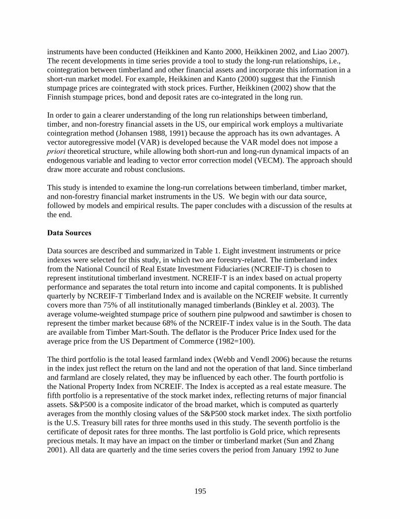
195

instruments have been conducted (Heikkinen and Kanto 2000, Heikkinen 2002, and Liao 2007). The recent developments in time series provide a tool to study the long-run relationships, i.e., cointegration between timberland and other financial assets and incorporate this information in a short-run market model. For example, Heikkinen and Kanto (2000) suggest that the Finnish stumpage prices are cointegrated with stock prices. Further, Heikkinen (2002) show that the Finnish stumpage prices, bond and deposit rates are co-integrated in the long run.

In order to gain a clearer understanding of the long run relationships between timberland, timber, and non-forestry financial assets in the US, our empirical work employs a multivariate cointegration method (Johansen 1988, 1991) because the approach has its own advantages. A vector autoregressive model (VAR) is developed because the VAR model does not impose a priori theoretical structure, while allowing both short-run and long-run dynamical impacts of an endogenous variable and leading to vector error correction model (VECM). The approach should draw more accurate and robust conclusions.

This study is intended to examine the long-run correlations between timberland, timber market, and non-forestry financial market instruments in the US. We begin with our data source, followed by models and empirical results. The paper concludes with a discussion of the results at the end. Data Sources Data sources are described and summarized in Table 1. Eight investment instruments or price indexes were selected for this study, in which two are forestry-related. The timberland index from the National Council of Real Estate Investment Fiduciaries (NCREIF-T) is chosen to represent institutional timberland investment. NCREIF-T is an index based on actual property performance and separates the total return into income and capital components. It is published quarterly by NCREIF-T Timberland Index and is available on the NCREIF website. It currently covers more than 75% of all institutionally managed timberlands (Binkley et al. 2003). The average volume-weighted stumpage price of southern pine pulpwood and sawtimber is chosen to represent the timber market because 68% of the NCREIF-T index value is in the South. The data are available from Timber Mart-South. The deflator is the Producer Price Index used for the average price from the US Department of Commerce (1982=100). The third portfolio is the total leased farmland index (Webb and Vendl 2006) because the returns in the index just reflect the return on the land and not the operation of that land. Since timberland and farmland are closely related, they may be influenced by each other. The fourth portfolio is the National Property Index from NCREIF. The Index is accepted as a real estate measure. The fifth portfolio is a representative of the stock market index, reflecting returns of major financial assets. S&P500 is a composite indicator of the broad market, which is computed as quarterly averages from the monthly closing values of the S&P500 stock market index. The sixth portfolio is the U.S. Treasury bill rates for three months used in this study. The seventh portfolio is the certificate of deposit rates for three months. The last portfolio is Gold price, which represents precious metals. It may have an impact on the timber or timberland market (Sun and Zhang 2001). All data are quarterly and the time series covers the period from January 1992 to June

196

2006. Due to the data constraint of the leased farmland index from NCREIF, each series has only 58 observations. Theoretical Framework Following the Johansen multivariate co-integration method (Johansen 1988, 1991, Johansen and Juselius 1990), a VAR model for asset returns was as follows:

tktktt XXX ε+Γ++Γ= −− ...11 (1) where X is a vector of variables, t is time index, k is the number of lags in the model, Γ is a matrix of parameter coefficients, and tε is a vector of error terms. If all variables are stationary, an unrestricted VAR system in level form could be employed. If all variables are non-stationary but no cointegration relationships exist, an unrestricted VAR system in first difference forms could be used. However, if all variables are nonstationary and cointegrated, the estimates obtained by the standard VAR model will be misspecified (Engle and Granger, 1987). To circumvent this problem, a VECM has been suggested (Harris 1995). Thus, it can be further reformulated into a vector error correction model as follows:

ttktktt XXXX ε+Π+∆Γ++∆Γ=∆ −−− 111 ... (2)

where Γ is a matrix of parameter coefficients for short-term dynamics and Π is a matrix of parameter coefficients. 'αβ=Π , where α can be interpreted as the speed of adjustment to disequilibrium, and β is a matrix of long-run coefficients. It is clear that all variables in first difference forms are stationary because all variables are unit root one I(1). The series tX'β is required to be stationary. Although Xt is nonstationary, the existence of co-integrating relationships indicates that the linear combinations of tX'β are indeed stationary and thus the columns of β form r distinct cointegrating vectors. The rank of Π is equal to the number of co-integration vectors. Thus, cointegration tests are to find the number of r linearly independent columns in Π (Harris 1995). The concept of cointegration indicates the existence of a long-run equilibrium to which an economic system converges over time (Harris 1995). It can be seen that the VECM model restricts the long-run behavior of the endogenous variables to revert to their equilibrium through the error correction term to adjust disequilibrium, while allowing a change of short-run dynamics. The modeling procedures are as follows: First, the stationary property of individual series is examined by the Augmented Dickey-Fuller (ADF) test (Enders 1995) because the data used in this study are time-series and may not be stationary. In addition, the number of lags should be determined because the VAR model is sensitive to lag selection. Furthermore, the trace and maximum Eigenvalue tests are used to detect the number of cointegration vectors. After determining the cointegration rank, the restriction tests are applied to long-run exclusion and weak exogeneity. If perfect integration exists among the variables, a multivariate test will be conducted by imposing restrictions on the cointegration vectors. Finally, diagnostic tests are conducted to examine the statistical adequacy of the models. The tests include the tests of normality, serial correction, and homoskedasticity for the residuals. Keep in mind that the

197

minimum requirement for an appropriate VAR model is the selected model is free of serial correlation in diagnostic tests (Doornik and Hendry 1994). In the empirical estimation, EViews 5.1 is used. Empirical Results Before the implementation of cointegration analysis, we need to examine if individual variables are nonstationary and integrated on the same order. The Augmented Dickey-Fuller (ADF) test was employed and the lag length for the test was determined by the Akaike Information Criterion (AIC). The results of the ADF test are reported in Table 2. The long-term government bond is excluded from the model because it is stationary. All other investment instruments are nonstationary and integrated of order one. Another requirement before performing the cointegration analysis is to determine the optimum lag length for the model. Three VAR systems were estimated; the first included timber alone (loggers or wood dealers) and other non-forestry financial instruments that consist of farmland return, real estate, stock index, treasure bill, certificate of deposit rate, and gold price. Instead of timber, the second model consisted of timberland alone (forest landowners) and the same non-forestry financial instruments. The third included both timber and timberland (forest industry processors) and the same non-forestry financial instruments. A number of VAR lag selection criteria were employed in the estimation. They are Log Likelihood Ratio (LR), Final Prediction Error (FPE), Akaike Information Criterion (AIC), Schwarz Information Criterion (SC), and Hannan-Quinn information Criterion (HQ) (EViews, 2004). For timber, LR suggests two lags, FPE and AIC indicate four lags, but SC and HQ indicate one lag,. For timberland, LR, FPE, and HQ conclude two lags, AIC indicates four lags, but SC suggests one lag. For both timber and timberland, LR, FPE, AIC, and HQ conclude four lags, but SC suggests one lag. The diagnostic tests then were conducted and lag lengths were set to two for timber, four for timberland, and four for timber and timberland because the VAR satisfied the minimum requirement for no serial correlation. The results of diagnostic tests for three VAR systems are available by request from the authors. The tests indicate that the residuals were not normally distributed due to excess kurtosis. This result is similar to the findings in Finland (Heikkinen 2002). Gonzalo (1994) suggests that cointegration results appear robust to excess kurtosis. Therefore, the models are acceptable, although they have this minor problem. Johansen’s multivariate cointegration analyses were explored for each of the three forestry-related investments. Two types of tests, the trace statistic and maximum Eigenvalue statistic, were used to detect the number of cointegrating vectors, r, which is an indictor of the extent of integration among variables. The results of the analyses are presented in Table 3. For timber, trace and maximum Eigenvalue tests show that the number of cointegration vectors is three, while six were found for timberland and for both timber and timberland. There is no statistical test to compare two different instruments for market integrations (Sun and Zhang 2006). We cannot say the conintegration result of 6 vectors is higher than the result of 3 vectors. However, it is reasonable to make such conclusions because the three models are similar in terms of time period, data source, and geographical coverage.

198

After determining the cointegration rank, the long-run exclusion tests are conducted for each financial instrument for three models. The null hypothesis states that an individual instrument can be excluded from the cointegration space. The tests are conducted by imposing restrictions on kr ,β of the r-th cointegrating relation, i.e., H0: 0, =krβ , r=1, 2, 3 for timber, but r=1,…, 6 for timberland and for timber and timberland models; k=1, …, 7 for timber and for timberland, but k=1, ..., 8 for timber and timberland, representing the corresponding variable equation in the cointegrating space. The test results are presented in Table 4. The null hypotheses are rejected in all cases. Therefore, none of these variables can be left out from the cointegration space and each variable has a long-run relationship with other variables in the system. The perfect cointegration test for the timberland model was conducted because it has six cointegration vectors and meet r=N-1. In addition, every pair of financial instruments must satisfy the parity condition (Sanjuan and Gil 2001, EViews 2004, and Sun and Zhang 2006). Thus, the hypothesis states H0: there is perfect integration among these portfolios for timberland model. This can be examined by putting restrictions on the cointegrating vectors in the VECM. Thus, the restrictions are

⎥⎥⎥⎥⎥⎥⎥⎥⎥

⎦

⎤

⎢⎢⎢⎢⎢⎢⎢⎢⎢

⎣

⎡

=×

1- 0 0 0 0 0 0 1- 0 0 0 0 0 0 1- 0 0 0 0 0 0 1- 0 0 0 0 0 0 1- 0 0 0 0 0 0 1- 1 1 1 1 1 1

67β (3)

where each column represents a cointegrating vector and each row denotes one equation in the VECM. This hypothesis satisfies the identification conditions and place one over-identifying restriction on each vector (Johansen and Juselius 1994, Sun and Zhang 2006). The Likelihood ratio statistics is 54.52 with a 2

)6(χ =12.59 distribution. The null hypothesis is rejected for the model. It reveals that there is no perfect integration, that is, investment changes in one instrument are not perfectly transmitted, although these portfolios are highly integrated. Finally, we need to examine if there are some leading or driving forces in the systems in the long run. We can test this by examining the weak exogeneity of each variable (Sanjuan and Gil 2001, Heikkinen 2002, Sun and Zhang 2006). Weak exogeneity means that a variable drives the system away from the long-run equilibrium errors, however, it cannot be affected by the other variables. In other words, the variable is dominant and plays a leading role in the system. The null hypothesis states there is a weak exogenous variable. The weak exogeneity for each portfolio in each model was examined by placing restrictions on the adjustment coefficient, rk ,α of the r-th cointegrating relation in the k-th VEC equation. That is, H0: rk ,α =0, k=1, …, 7 for timber and for timberland, but k=1, ..., 8 for timber and timberland; r=1, 2, 3 for timber, but r=1,…, 6 for timberland and for timber and timberland models. The likelihood ratio statistics have a chi-square distribution and the degree of freedom is equal to the number of cointegrating vectors.

199

The test results are presented in Table 5. For timberland and for both timber and timberland models, all statistics are significant at the 5% level and null hypotheses are rejected for these two models. Therefore, there are no driving financial instruments in the two models. Surprisingly, for the timber model, deposit interest rate and gold price are weak exogenous variables, which play leading roles in the model. The result for deposit rate is similar to the finding in Finland (Heikkinen 2002), although in most of the cases, no variables are weakly exogenous.

Conclusion and Discussion Using cointegration analysis, we examine the long-run correlations among timberland, timber market and non-forestry financial instruments in the US. The results with cointegration analysis reveal that there might exist cointegrated relationships between timberland, timber price, and the non-forestry financial assets in the long run. This also means that investment should be low risk, low return or high risk, high return. Within the long run relationships, the results show that no financial instrument is excluded from the model systems, there is no perfect integration for timberland model, and no driving variables are identified for timberland and for both timber and timberland models. These findings make a contribution to the literature gap in two major aspects. First, the long run relationships between timberland return, timber, and financial assets are examined using multivariate cointegration method. The approach should draw more accurate and comprehensive conclusions. Second, diversified financial instruments provide risk-reducing benefits for the portfolio investors. This study uses eight financial instruments whereas previous studies have limited financial selections (e.g. Heikkinen and Kanto 2000, Heikkinen 2002). The results may have policy and welfare implications. First, timber investors might consider portfolio strategy in both the short run and the long run because, although forestry-related investments and financial asset have no close relationships in the short run, they might have cointegrated relationships in the long run. Second, for policy makers, it is better to consider all the eight markets simultaneously because any policy change in one market will potentially spill over onto the other markets and have welfare implications in the long run. Further research is needed to examine the long-run relationship between forestry-related assets and other non-forestry financial assets at regional level, considering the large variations in asset investments in the conterminous US.

Literature Cited Binkley, C.S., C.F. Raper and C.L. Washburn. 1996. Institutional ownership of US timberland.

History, rationale and implications for forest management. J. For. 94(9) 21–28. Binkley, C.S., C.L. Washburn, M.E. Aronow, and T. Fritzinger. 2003. Timberland Investment

Performance. Hancock Timberland Investor. Bureau of Labor Statistics. 2006. The producer price index (PPI). http://www.bls.gov/ppi Clutter, M., B. Mendell, D. Newman, D. Wear, and J. Greis. 2005. Changing forest ownerships

in the South. University of George, Warnell School of Forest Resources. In Process.

200

Doornik, J., and D. Hendry. 1994. Interactive econometric modeling of dynamic system (PcFiml 8.0). Institute of Econ. and Stati., University of Oxford. London: International Thomson Publishing. 436 p.

Enders, W. 1995. Applied econometric time series. John Wiley & Sons, Inc., New York. 433 p. Engel, R.F., and C.W.J. Granger. 1987. Cointegration and Error Correction: Representation,

Estimation, and Testing. Econometrica, vol. 55, pp. 251-276. EViews. 2004. Eviews User’s Manual. Quantitative Micro Software. Federal Reserve Bank. 2006. Historical database of economic and financial data. http://www.federalreserve.gov/releases/h15 Gonzalo, J. 1994. Five alternative methods of estimating long-run equilibrium relationships. J.

Econ. 60:203-233. Harris, R. 1995. Using Co-integration Analysis in Econometric Modeling. London, UK: Prentice

Hall. 176 p. Heikkinen, V-P. 2002. Co-integration of timber and financial assets—implications for portfolio

selection. For. Sci. 48(1) 118–128. Heikkinen, V-P., and A. Kanto. 2000. Market model with long-term effects—empirical evidence

from Finnish forestry returns. Silva Fennica 34(1) 61–69. Johansen, S. 1988. Statistical analysis of co-integrating vectors. J. Econ. Dynam. Contr. 12 231–

254. Johansen, S. 1991. Estimation and hypothesis testing of cointegration vectors in Gaussian vector

autoregressive models. Econometrica 59 (November): 1551-80. Johansen, S., and K. Juselius. 1990. Maximum likelihood estimation and inference on

cointegration with applications to demand of demand. Oxford Bulletin of Econ. and Stat. 52 (May): 169-210.

Johansen, S., and K. Juselius. 1994. Identification of the Long-run and the Short-run Structure:

An Application to the ISLM Model. J. of Econometrics 63: 7-36. Liao, X. 2007. Essays of Forestry Investments in the US and Stumpage Market in the Southern

US. PhD Dissertation. Auburn University. 98 p. National Council of Real Estate Investment Fiduciaties (NCREIF). 2006. The NCREIF

Timberland Index detailed quarterly Performance Report. http:///www.ncreif.com/indices/timberland.htp.

201

Redmond, C.H., and F.W. Cubbage. 1988. Portfolio risk and returns from timber asset investment. Land Econ. 64(4) 325–337.

Sanjuan, A., and J.M. Gil. 2001. A note on tests for market integration in a multivariate non-

stationary framework. J. Agric. Econ. 52(2):113-121. Smith, W. B., P. D. Miles, J. S. Vissage, and S. A. Pugh. 2004. Forest resources of the United

States, 2002. U.S. Department of Agriculture, Forest Service, North Central Research Station, St. Paul, MN. Gen. Tech. Rep. NC-241. 137 pp.

Sun, C., and D. Zhang. 2001. Assessing the Financial Performance of Forestry-Related

Investment Vehicles: Capital Asset Pricing Model vs. Arbitrage Pricing Theory. Am. J. Agric. Econ. 83(3):617-628.

Sun, C., and D. Zhang. 2006. Market Structure and Timber Harvesting Margins in the U.S.

South: A Temporal and Spatial Analysis. For. Sci. 52(3):273-280. The Financial Forcast Center (FFC). 2006. Business, finance, & economic data.

http://www.forecasts.org/data. Thomson, T.A. 1989. Evaluating some financial uncertainties of tree improvement using the

capital asset pricing model and dominant analysis. Can. J. For. Res. 19:1380-1388. Timber Mart-South. Quarterly report of the market prices for timber products of the Southeast

from 1977 to 2006. Highlands NC: Timber Mart-South, Inc. Washburn, C.L., and C.S. Binkley. Do forest assets hedge inflation? Land Econ. 69:215-224. Webb, R.B., and R. Vendl. 2006. Total leased farmland data. Personal communication. Wooldridge, J.M. 2000. Introductory econometrics: A modern approach. South-Western College

Publishing, Boston, MA. 824 p.

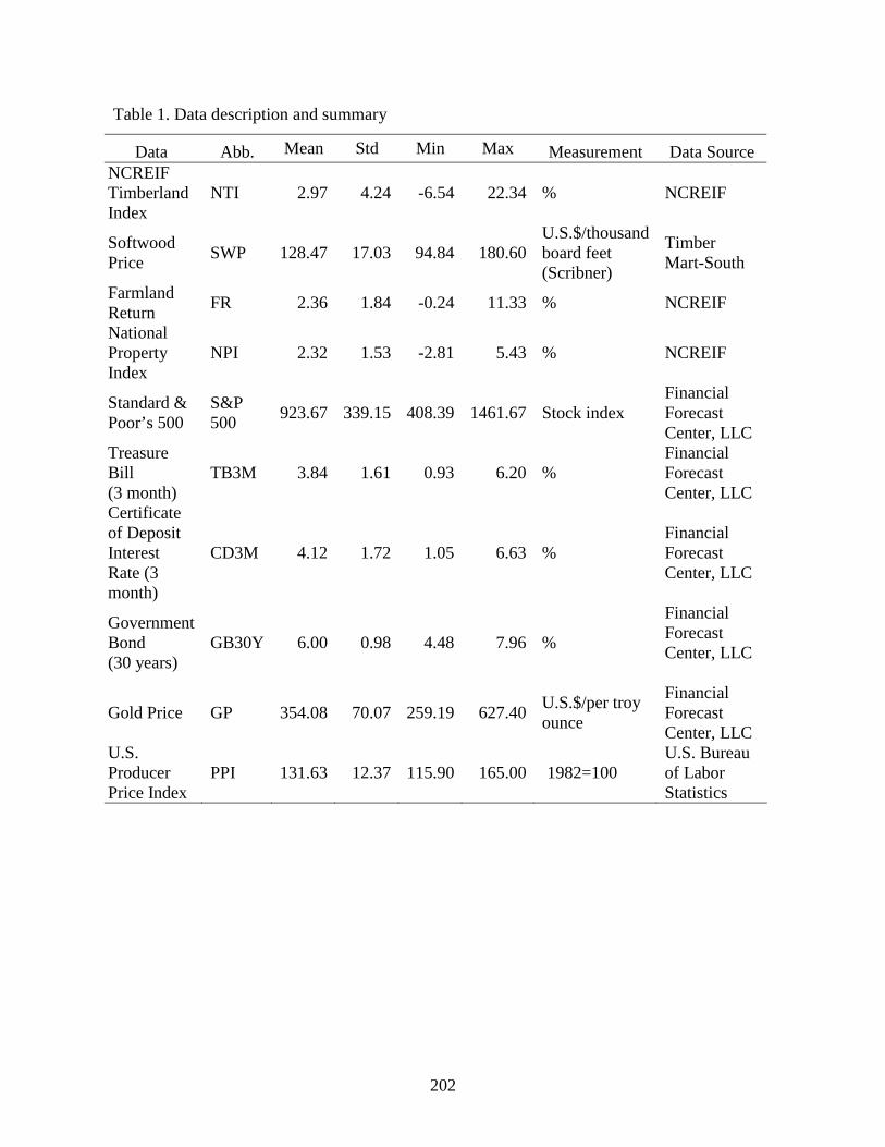
202

Table 1. Data description and summary

Data Abb. Mean Std Min Max Measurement Data Source NCREIF Timberland Index

NTI 2.97 4.24 -6.54 22.34 % NCREIF

Softwood Price SWP 128.47 17.03 94.84 180.60

U.S.$/thousand board feet (Scribner)

Timber Mart-South

Farmland Return FR 2.36 1.84 -0.24 11.33 % NCREIF

National Property Index

NPI 2.32 1.53 -2.81 5.43 % NCREIF

Standard & Poor’s 500

S&P 500 923.67 339.15 408.39 1461.67 Stock index

Financial Forecast Center, LLC

Treasure Bill (3 month)

TB3M 3.84 1.61 0.93 6.20 % Financial Forecast Center, LLC

Certificate of Deposit Interest Rate (3 month)

CD3M 4.12 1.72 1.05 6.63 % Financial Forecast Center, LLC

Government Bond (30 years)

GB30Y 6.00 0.98 4.48 7.96 %

Financial Forecast Center, LLC

Gold Price GP 354.08 70.07 259.19 627.40 U.S.$/per troy ounce

Financial Forecast Center, LLC

U.S. Producer Price Index

PPI 131.63 12.37 115.90 165.00 1982=100 U.S. Bureau of Labor Statistics

203

Table 2. Results of ADF unit-root tests

Series Level First Difference Lags NTI -3.05 -7.96** 3 SWP -2.32 -5.06** 6 FR -1.99 -8.79** 5 NPI -2.41 -4.94** 2 SP500 -2.06 -5.75** 3 TB3M -2.76 -3.35* 6 CD3M -3.02 -3.42* 2 GB30Y -5.66** 3 GP 1.76 -4.00** 1

Note: 1. See Table 1 for definitions of the variables 2. ** and * denote rejection of null hypothesis of a unit root at 5% and 10% significant

level. 3. The 5% and 10% critical values for the ADF including a constant and a linear trend

are -3.50 and –3.18 4. The lag lengths were chosen on the basis of the Akaike information criteria.

Table 3. Trace and maximum Eigenvalue tests for cointegration rank

Timber Timberland Timber & Timberland

H0 Trace Max Trace Max Trace Max

R=0 165.46** 52.32** 331.23** 130.08** 591.79** 197.49**

R=1 113.14** 42.85** 201.15** 78.36** 394.31** 128.28**

R=2 70.28** 35.36** 122.79** 47.77** 266.02** 123.33**

R=3 34.92 14.85 75.01** 29.32** 142.70** 64.32**

R=4 20.08 12.5 45.70** 23.31** 78.38** 39.22**

R=5 7.58 7.55 22.39** 18.74** 39.17** 23.75**

R=6 0.03 0.03 3.65 3.65 15.41 14.94**

R=7 0.47 0.47

R 3 3 6 6 6 7

Note:

1.** denotes rejection of the hypothesis at the 5% level

2. Two lags for timber, four lags for timberland, and for both timber & timberland.

204

Table 4. Test results for long-run exclusion

Variable Timber

2)3(χ =7.81

Timberland 2

)6(χ =12.59 Timber & Timberland

2)6(χ =12.59

SWP 23.82** 96.98** NTI 36.31** 82.07** FR 22.13** 40.60** 117.66** NPI 28.18** 38.29** 105.81** SP500 29.21** 31.91** 132.53** TB3M 26.05** 72.29** 164.91** CD3M 26.03** 73.47** 165.54** GP 27.09** 58.96** 95.68**

Note: The likelihood ratio tests have a 2χ distribution and the degree of freedom is equal

to the number of cointegrating vectors. ** indicates significant at the 5% level.

Table 5. Likelihood ratio tests of weak exogeneity

Variable Timber

2)3(χ =7.81

Timberland 2

)6(χ =12.59 Timber & Timberland

2)6(χ =12.59

SWP 6.35* 26.74** NTI 33.08** 25.45** FR 28.64** 27.24** 14.40** NPI 25.42** 36.46** 95.12** SP500 16.39** 22.17** 20.95** TB3M 7.27* 17.30** 25.00** CD3M 5.13 16.96** 12.93** GP 2.22 55.36** 44.39**

Note: The likelihood ratio tests have a 2χ distribution and the degree of freedom is equal to the

number of cointegrating vectors. ** and * indicate significant at the 5% level and 10% level, respectively.

205

An Empirical Analysis of Timberland Ownership and Corporate Financial Performance for Forestry Industries in the U.S.

Yanshu Li and Daowei Zhang1

Abstract: This study presents an empirical analysis of the relationship between industrial timberland ownership and financial performance of forestry products companies in the U.S. A three stage least square (3SLS) model system was used for estimation. The results show that generally timberland holding may improve a forestry products company’s profitability in terms of ROA and ROE and its ability of response of rate of returns to uncertainty. Large firms were shown to be more likely have higher ROE and ROA at the expense of higher systematic risk than that of small firms. Forest product companies may divest some of their timberland to ease the financial burden. When the return of timberland is high, forestry product firms are inclined to decrease their timberland holdings.

Keywords: Industrial timberland ownership, forestry products industry, financial performance, 3SLS

1 Respectively, Postdoctoral Fellow and Professor, School of Forestry and Wildlife Sciences, Auburn University, AL 36849, zhangdw@auburn.edu (D. Zhang), (334) 844-1067 (v).

206

The Location Theory Dilemma in the Forest Products Industry: What Site-attributes Are Considered for the Establishment of Softwood Sawmills?

Francisco X. Aguilar1 and Richard P. Vlosky2 Abstract: The forest products industry in the U.S. has experienced a shift in manufacturing from the Northeast to the Pacific Northwest and the Southern region. But, what attributes are the most important when considering when to locate a resource-based manufacturing facility? A nationwide survey of plant managers and owners was carried to elicit site preferences for softwood sawmills. A dual approach applying a choice-based conjoint and multiple-choice factor analyses is applied to the decision-maker location dilemma. The factor analysis helps identify the most important “categories” of attributes (e.g. log supply, input costs, environmental legislation), and the conjoint analysis attempts to assign relative weights to selected attributes. Results are accompanied with a discussion of its implications toward future developments in the forest products industry.

1 Ph.D. candidate at the School of Renewable Natural Resources, Louisiana State University Agricultural Center. Baton Rouge, LA, 70803, faguil1@lsu.edu. 2 Director of the Louisiana Forest Products Development Center and Professor of Forest Products Marketing at the School of Renewable Natural Resources, Louisiana State University Agricultural Center. Baton Rouge, LA, 70803, vlosky@lsu.edu.

207

Measuring the Biological and Economic Effects of Wildlife Herbivory on Afforested Carbon Sequestration Sites in the Lower Mississippi Alluvial Valley

Daniel C. Sumerall, Donald L. Grebner, Jeanne C. Jones, Keith L. Belli, Stephen C. Grado, and Richard P. Maiers1

Abstract: It has been suggested that afforestation of marginal or abandoned agricultural lands in the Lower Mississippi Alluvial Valley (LMAV) with bottomland hardwoods offers the greatest opportunity for significant net carbon storage in the southern United States. In February 2006, Mississippi State University and Entergy began a carbon sequestration study in the LMAV by afforesting 36 acres of retired agricultural land in western Mississippi. One of the primary causal factors of failed and delayed reforestation attempts in the LMAV is mammalian herbivory. Herbivory of seedlings generally reduces growth and often leads to seedling mortality. A study was designed to determine the biological and economic impacts of mammalian herbivory on these afforested sites. The experiment is a completely randomized 6 x 2 x 2 factorial design, in which seedlings were planted using six species mixes with two fertilizer treatments (fertilized or unfertilized) and two competition treatments (herbicide or no herbicide). Seedlings from each species mix and fertilizer/herbicide combination were randomly selected for monitoring throughout the first growing season. Growth, survival, and herbivory data were recorded for each selected seedling. Utilizing this biological data as well as known establishment and treatment costs, land expectation values (LEV) will be compared to determine the feasibility of each planting mix and treatment combination. Through this research, we hope to identify a cost-effective species mix that can be utilized in the LMAV to promote carbon sequestration and withstand the potential negative impacts associated with browsing by mammalian herbivores. Keywords: Bottomland hardwoods, browsing, herbivory, Lower Mississippi Alluvial Valley, Mississippi Delta, regeneration delay

1 Respectively, Graduate Research Assistant, Associate Professor, Associate Professor, Associate Dean and Professor, Professor, and Assistant Professor, Forest and Wildlife Research Center, Box 9681, Mississippi State, MS 39760, dcs48@msstate.edu (D. Sumerall).

208

A Case Study to Examine How a Forestry Firm Might Respond to Different Mechanism to Encourage Carbon Sequestration

Patrick Asante1

Abstract: Despite considerable interest in the potential for forests to sequester carbon, there is still a gap in knowledge when it comes to determining the effect of carbon credit trading on forestry firms as it relates to harvest/leave decisions, reforestation options, and afforestation of agricultural land. Managing forest for carbon budget may result in modifications to the way forests are managed in Canada depending on the incentives provided by carbon markets. Utilizing the southwestern portion of Daishowa-Marubeni International Ltd. (DMI) forest management area (FMA) in Peace River, Alberta, as a case study, from the perspective of a carbon credit supplier, a mathematical programming model is used to evaluate how carbon price, silvicultural practices, supply of carbon credits, and allowable annual cut regulations could affect a forestry firms decision to undertake enhanced carbon sequestration. The knowledge gained through this research will enter into national policy discussions regarding carbon management, and will inform relevant agencies about how forestry firms might respond to different mechanisms that seek to encourage carbon sequestration. Results and methods from this study should give forestry firms the building blocks to develop strategic plans for managing their forest for carbon budget. Keywords: Carbon sequestration, mathematical programming model, carbon sinks, carbon budget

1 University of Alberta, Canada, Patrick.Asante@afhe.ualberta.ca.

209

Linking Attitude and Subjective Norm to Intention and Fire Use Behavior: The Case of the Wu-Lin District, Taiwan

Hsiaohsuan Wang1, 2, Jianbang Gan2, Chyirong Chiou3, and Chauchin Lin4 Abstract: People living in a forest district have close interactions with the forest. Their fire use behavior is often one of the key fire hazards. Therefore, a good understanding and analysis of their fire use behavior would be helpful in preventing forest fires. This study estimates the relationship between fire use behavior and intention that is further related to attitude and subjective norm for residents in the Wu-Lin district, Taiwan according to the Theory of Reasoned Action. Such relationships are helpful in developing strategies to alleviate future wildfire risk in the area. Keywords: Forest fire, the Theory of Reasoned Action, behavior, intention, attitude, subject norm

1 Corresponding author and presenter, hsuan006@neo.tamu.edu. 2 Department of Ecosystem Science and Management, Texas A&M University, College Station, TX 77843-2138. 3 National Taiwan University. 4 Taiwan Forestry Research Institute.

210

An Evaluation of the Economic Potential of Surface Mined Areas for Tree Production

Adam Michels1, Tamara Cushing2, Christopher Barton3, Jim Ringe4, Patrick Angel5, Rick Sweigard6, and Donald Graves7

Abstract: After the passage of The Surface Mining Control and Reclamation Act of 1977 (SMCRA), federal surface mine regulators focused primarily on the stability of reclaimed land rather than reforestation of that land. This has resulted in thousands of acres of compacted reclaimed land not hospitable to tree growth. Most surface mines are reclaimed for pasture or wildlife land uses and are graded smooth and planted in aggressive groundcover. Pre-law strip mines were not graded and compacted, but simply had the overburden dumped. These sites have been able to establish productive forest cover. In Appalachia, including Kentucky, methods of ripping the soil to ameliorate compaction on previously reclaimed mines have been used in order to create a more hospitable environment for tree growth. Four methods to reduce compaction on reclaimed surface mines were compared at the Bent Mountain research site in Pike County, Kentucky. The methods included: single shank ripped spoil, triple shank ripped spoil, excavated spoil, and rough graded spoil. Normally graded spoil was also examined as a control to represent a traditional reclamation practice. I calculated the land expectation value (LEV) for each reclamation method including the one time reclamation costs for the first rotation. The discount rate was varied in order to test the sensitivity of the LEV formula to different discount rates. The LEV can provide us with the economic potential of a reclaimed surface mine to produce timber, and show where subsidies for reforestation may be needed to reforest some surface mines. Keywords: Surface mining, land expectation value, reclamation

1 Graduate Student, Department of Forestry, University of Kentucky, Lexington, KY 40506, acmich2@uky.edu. 2 Assistant Professor, Department of Forestry, University of Kentucky, Lexington, KY 40506, Tamara.Cushing@uky.edu. 3 Assistant Professor, Department of Forestry, University of Kentucky, Lexington, KY 40506, barton@uky.edu. 4 Professor, Department of Forestry, University of Kentucky, Lexington, KY 40506, jringe@pop.uky.edu. 5 Forester/Soil Scientist, Office of Surface Mining Reclamation and Enforcement, U.S. Department of Interior, pangel@osmre.gov. 6 Chair and Professor, Department of Mining Engineering, University of Kentucky, Lexington, KY 40506, rsweigar@engr.uky.edu. 7 Extension Professor Emeritus and Retired Chair, Department of Forestry, University of Kentucky, Lexington, KY 40506, dgraves@uky.edu.

211

Property Taxation and Forest Fragmentation in Kentucky Watersheds

Scott Brodbeck1 and Tamara Cushing2

Abstract: This study examines the current practices utilized in assessing forest land for property tax purposes in thirty-seven counties in the Green River and the Lower Cumberland River Watersheds in Kentucky. These watersheds are among the top fifteen watersheds in the United States expected to experience increased development and fragmentation according to the U. S. Forest Service. The goal is to build a foundation for future studies related to forest land taxation and for changes in tax policy to promote sustainable forest management. By promoting forest management through tax policy the rate of fragmentation and conversion of forest lands to other uses may be reduced. A survey was conducted with the property valuation administrators for the counties in the Green River and Lower Cumberland River Watersheds. The survey provides data on how properties are valued for taxation in each county. After the valuation methods were identified and grouped they were applied to a hypothetical property that could be found in the watersheds to allow for the comparison of the net present value under different assessment methods. A sensitivity analysis was performed to determine the impact of each of the assumptions used in calculating net present values.

1 Graduate Research Assistant, University of Kentucky, Forestry Department, 105 T.P. Cooper Building, Lexington, KY 40546-0073, scott.brodbeck@uky.edu, (859) 257-9773 (v.). 2 Assistant Professor, University of Kentucky, Forestry Department, 104 T.P. Cooper Building, Lexington, KY 40546-0073, tamara.cushing@uky.edu, (859) 257-2149 (v).

212

A Comparison of Taxes Incurred During the Production and Delivery of Hardwood Sawtimber in Kentucky, Maryland, Virginia, and West Virginia

Kathryn Arano1 and Stuart Moss2 Abstract: Investment levels in the forestry sector are affected by the tax cost associated with timberland ownership, forestland management, and conversion of timber into saleable products. While taxes are a major source of revenues for state and local governments, they impose a cost on landowners, on industries, and on other players in the wood production chain. Tax structures among states may vary significantly. Local businesses like wood industries may face a different tax burden depending on where they are located. This report examines the tax burden of the wood industry in West Virginia compared to surrounding states. Because of data and time limitations, the analysis is limited to West Virginia and three adjoining states – Kentucky, Maryland, and Virginia. This report specifically focuses on three types of taxes incurred during the production of hardwood sawtimber and its delivery to a processing mill: real property, motor fuel, and yield / severance. Total sawtimber production taxes in Kentucky, Maryland, and Virginia are $8.93, $16.16, and $10.37 per MBF, respectively. By comparison, total sawtimber production taxes in West Virginia were $17.20 / MBF in 2005 and are expected to increase to $21.29 / MBF with the additional “severance” (yield) tax that began in December 2005. With this additional tax, total timber taxes in West Virginia will be about 32% higher than Maryland and more than twice as high as those in Kentucky and Virginia.

1 Assistant Professor, Division of Forestry and Natural Resources, West Virginia University, P.O. Box 6125, Morgantown, WV 26506, (304) 293-2941, Kathryn.Arano@mail.wvu.edu 2 Research Assistant Professor, Division of Forestry and Natural Resources, West Virginia University, P.O. Box 6125, Morgantown, WV 26506

213

Spatial Analysis of Economic Freedom, Corruption, and Species Imperilment at Cross-country Level

Ram Pandit1 and David N. Laband2

Abstract: Using spatial regression and cross-national data from 152 countries a direct empirical link is explored between the impact of economic freedom and corruption on species imperilment for 5 taxa groups: birds, mammals, reptiles, amphibians, and vascular plants. The analysis suggests that there are statistically significant relationships between imperilment of birds, mammals, and reptiles and economic freedom. However, the relationship between corruption and species imperilment is found significant only among birds. More economic freedom and less corruption after a threshold level reduce species imperilment in a country.

1 Ph.D. Candidate, Center for Forest Sustainability, School of Forestry and Wildlife Sciences, Auburn University, 602 Duncan Drive, Auburn University, AL 36849-5418, pandira@auburn.edu, (334) 844-8026 (v). 2 Professor, Center for Forest Sustainability, School of Forestry and Wildlife Sciences, Auburn University, 602 Duncan Drive, Auburn University, AL 36849-5418.

214

Breeching the Biomass Barriers: Analyzing Policy Effectiveness and Rectifying Disjuncture between Biomass Utilization and Hazardous Fuel Mitigation on NIPF Land

Adam Jarrett1, 2 and Jianbang Gan2 Abstract: Wildfire has become an increasing concern by nonindustrial private forestland owners in the U.S. South. This study assesses the landowners’ awareness of state wildfire mitigation assistance programs and their attitude toward and action in wildfire mitigation. A landowner survey is conducted in five southern states including Alabama, Georgia, Florida, Mississippi, and South Carolina. The factors influencing landowners’ awareness, attitude, and action are identified using logit regression. Our results offer suggestions for improving the effectiveness of these state wildfire mitigation programs.

Keywords: Wildfire mitigation, landowner assistance, southern U.S.

1 Graduate Research Assistant and presenter, jarrett1@neo.tamu.edu. 2 Department of Ecosystem Science and Management, Texas A&M University, College Station, TX 77843-2138.

215

Conference Program

2007 SOFEW GLOBAL CHANGE AND FORESTRY: ECONOMIC AND POLICY IMPLICATIONS

Sunday, March 4 6:00-9:00 PM REGISTRATION – Guest Relations Monday, March 5 7:00 AM REGISTRATION – Peraux Foyer CONTINENTAL BREAKFAST - Peraux 8:00 GENERAL SESSION I – Peraux (Moderator: Steve Whisenant) Welcome – Steve Whisenant, Texas A&M University

Climate change effects and mitigation: Forestry economic consequences and modeling, ramblings from an ongoing and never ending effort – Bruce A. McCarl, Texas A&M Univeristy

Global change in fiber markets: Impacts on U.S. pulpwood outlook – Peter Ince, USDA Forest Products Laboratory

9:40 BREAK - Peraux 10:00 GENERAL SESSION II – Peraux (Moderator: Jianbang Gan)

Future of forest economics and policy research – Gregory S. Amacher, Virginia Polytechnic Institute and State University; David H. Newman, University of Georgia; David N. Wear, USDA Forest Service; and Daowei Zhang, Auburn University

11:30 LUNCH – Georgian 1:00 PM CONCURRENT SESSIONS A

A1 – Climate Change and Land Use – LaSalle (Moderator: Donald G. Hodges) Forest management adaptation to climate change and extreme events. Jin Huang and Bob Abt, North Carolina State University

216

A case study to examine how a forestry firm might respond to different mechanism to encourage carbon sequestration. Patrick Asante, University of Alberta Impact of population growth and urban sprawl on land use and forest type dynamics along urban-rural gradient. Maksym Polyakov and Daowei Zhang, Auburn University Impacts of climate change on Tennessee forests. Donald G. Hodges, University of Tennessee; Virginia H. Dale, Oak Ridge National Laboratory ; and Jonah Fogel, University of Tennessee

A2 – Forest Products Markets I – Alamo (Moderator: Sun Joseph Chang) How competitive is the wood supply chain in the U.S. South? Jacek P. Siry, W. Dale Greene, Thomas G. Harris, Jr., and Robert L. Izlar, University of Georgia Is the current poor market for hardwood lumber in North Carolina, Virginia, and West Virginia temporary? William Luppold and Matthew Bumgardner, USDA Forest Service An econometric analysis of pine pulpwood market in the Southern US. Xianchun Liao and Yaoqi Zhang, Auburn University A review of econometric models for softwood lumber. Nianfu Song and Sun Joseph Chang, Louisiana State University

A3 – Nonindustrial Private Forests I – LaFitte (Moderator: Ian Munn) Unintended consequences: Effect of the American Jobs Creation Act reforestation incentives on family forest owners in the South. John L. Greene, USDA Forest Service; and Thomas J. Straka, Clemson University Impacts of Timberland Ownership on Stumpage Market in the US South. Yaoqi Zhang and Xianchun Liao, Auburn University Forest management decisions of nonindustrial private forest landowners of West Virginia. Sudiksha Joshi and Kathryn G. Arano, West Virginia University Nonindustrial private forest landowners’ participation in Mississippi Forest Resource Development Program. Xing Sun, Changyou Sun, Ian A. Munn, and Anwar Hussain, Mississippi State University

3:00 BREAK – Peraux

217

3:20 CONCURRENT SESSIONS B

B1 – Bioenergy – LaSalle (Moderator: Donald L. Grebner) Biofuel production impact on the management of southern pine plantation in Mississippi. Zhimei Guo, Donald L. Grebner, Changyou Sun, and Stephen C. Grado, Mississippi State University Woody biomass feedstock supplies and management for bioenergy in southwestern Mississippi. Gustavo Perez-Verdin, Donald Grebner, Changyou Sun, Ian Munn, Emily Schultz, and Thomas Matney, Mississippi State University A forest product/bioenergy mill location and decision support system based on a county-level forest inventory and geo-spatial information. T. Luke Jones, Emily B. Schultz, Thomas G. Matney, Donald L. Grebner, and David L. Evans, Mississippi State University Logging residues as a source of bioenergy feedstock. Robert K. Grala, Laura A. Grace, and William B. Stuart, Mississippi State University To burn or not to burn. Sun Joseph Chang, Louisiana State University B2 – Forest Products Markets II – Alamo (Moderator: Weihua Xu) Measuring oligopsony and oligopony power in the U.S. paper industry. Bin Mei and Changyou Sun, Mississippi State University Testing the efficiency of spatial arbitrage between North American softwood lumber markets of homogeneous products. Chander Shahi and Shashi Kant, University of Toronto

A time series analysis of lumber market in US South. Ram Pandit and Indrajit Mujumdar, Auburn University An analysis of quarterly composite hardwood sawtimber price indices: 1998-2006. Chris Zinkhan, Blake Stansell, and Thresa Henderson, The Forestland Group, LLC Hardwood lumber demand:1963 to 2002. William Luppold and Matthew Bumgardner, USDA Forest Service

218

B3 – Economic Impact and Development – LaFitte (Moderator: Tamara Cushing) Economic impact associated with Mississippi outfitters and their clientele. Anwar Hussain and Ian A. Munn, Mississippi State University The economic impacts of two birding festivals in Mississippi. Marcus K. Measells and Stephen C. Grado, Mississippi State University An Introduction to the Southern US Wood Supply System: A Value Chain Approach. Clayton B. Altizer, Mississippi State University

Forest-based economic development in Arkansas: A case for the forest products industry. Matthew H. Pelkki, University of Arkansas-Monticello

Development of a south-wide forest economics dataset for the Southern Forest Research Partnership. Matthew Pelkki, University of Arkansas-Monticello

6:00 RECEPTION – Peacock Alley POSTER SESSION – Peacock Alley (Coordinator: Weihua Xu)

Measuring the biological and economic effects of wildlife herbivory on afforested carbon sequestration sites in the lower Mississippi alluvial valley. Daniel C. Sumerall, Donald L. Grebner, Jeanne C. Jones, Keith L. Belli, Stephen C. Grado, Richard P. Maiers, Mississippi State University A case study to examine how a forestry firm might respond to different mechanism to encourage carbon sequestration. Patrick Asante, University of Alberta Linking attitude and subjective norm to intention and fire use behavior: The case of the Wu-Lin district, Taiwan. Hsiaohsuan Wang and Jianbang Gan, Texas A&M University; Chyirong Chiou, National Taiwan University; and Chauchin Lin, Taiwan Forestry Research Institute An evaluation of the economic potential of surface mined areas for tree production. Adam Michels, Tamara Cushing, Christopher Barton, Jim Ringe, Patrick Angel, Rick Sweigard, and Donald Graves, University of Kentucky

Property taxation and forest fragmentation in Kentucky watersheds. Scott Brodbeck and Tamara Cushing, University of Kentucky A comparison of taxes incurred during the production and delivery of hardwood sawtimber in Kentucky, Maryland, Virginia, and West Virginia. Kathryn Arano and Stuart Moss, West Virginia University

219

Spatial analysis of economic freedom, corruption, and species imperilment at cross-country level. Ram Pandit and David N. Laband, Auburn University Breeching the biomass barriers: Analyzing policy and cost effectiveness for wildfire mitigation and biomass utilization. Adam Jarrett and Jianbang Gan, Texas A&M University

Tuesday, March 6 7:00 AM BUSINESS MEETING - Coronado CONTINENTAL BREAKFAST – Peacock Alley 8:00 CONCURRENT SESSIONS C

C1 – Recreation – LaSalle (Moderator: Stephen C. Grado) Recreational visitation patterns on lake impoundments in east-central Mississippi. Jon P. Rezek and Stephen C. Grado, Mississippi State University Factors determining per acre market value of hunting leases on Sixteenth Section Lands in Mississippi. Jacob Rhyne, Mississippi State University Influence of field windbreaks on landscape aesthetics: Preliminary results. Robert K. Grala and John C. Tyndall, Mississippi State University; and Carl W. Mize, Iowa State University

C2 – Conservation I – Alamo (Moderator: Weihua Xu) Factor driving deforestation in common-pool resources in Durango, Mexico. Gustavo Perez-Verdin, Mississippi State University; and Yeon-Su Kim, Denver Hospodarsky, and Aregai Tecle, Northern Arizona University Determinants of forest preservation. J.A. Anderson1, M.K. Luckert, and W.L. Adamowicz, Univeristy of Alberta A marginal cost analysis of trade-offs in preservation of old growth in an even aged boreal forest of Ontario. Rajender P. Khajuria and Susanna Laaksonen-Craig, University of Toronto Globalization, market economy and tropical deforestation: Evidence from Southwest China. Youxin Ma, Chinese Academy of Sciences; Yaoqi Zhang, Auburn University; and Hongmei Li, Wenjun Liu, and Min Cao, Chinese Academy of Sciences

220

C3 – Nonindustrial Private Forests II – LaFitte (Moderator: Lawrence D. Teeter) How long do NIPF landowners wait to reforest after harvesting. Xing Sun, Ian A. Munn, and Changyou Sun, Mississippi State University

Analysis of family forest holdings structure in the United States. Yaoqi Zhang and Xianchun Liao, Auburn University; and Brett J. Butler, USDA Forest Service Timber harvest behavior of nonindustrial private forest (NIPF) landowners facing uncertainty from an insect pest: The case of the red oak borer. G.C. Surendra and Sayeed R. Mehmood, University of Arkansas-Monticello

Discriminating family forest owner groups using a non-parametric approach. Indrajit Majumdar and Lawrence D. Teeter, Auburn Univeristy; and Brett J. Butler, USDA Forest Service

10:00 BREAK – Peacock Alley 10:20 CONCURRENT SESSIONS D

D1 – Finance and Industry Location – LaSalle (Moderator: John L. Greene) Investment analysis and timberland portfolios in the US. Xianchun Liao and Yaoqi Zhang, Auburn University An empirical analysis of timberland ownership and corporate financial performance for forestry industries in the US. Yanshu Li and Daowei Zhang, Auburn University

The location theory dilemma in the forest products industry: What site-attributes are considered for the establishment of softwood sawmills? Francisco X. Aguilar and Richard P. Vlosky, Louisiana State University

D2 – Conservation II – Alamo (Moderator: Jay Sullivan) Performance bonding and reforestation of surface mined lands. Jay Sullivan and Greg Amacher, Virginia Polytechnic Institute and State University

Evaluation of cogongrass control techniques for nonindustrial private landowners in Mississippi. Jon D. Prevost, Donald L. Grebner, Jeanne C. Jones, Stephen C. Grado, Keith L. Belli, and John Byrd, Mississippi State University

221

Economic impact of the forest policy in Uruguay. Virginia Morales, University of Georgia

D3 – Valuation – LaFitte (Moderator: Matthew Pelkki) Willingness-to-pay assessment of visitors to an off-highway vehicle recreation area: An individual travel cost method approach. Gregory Parent, Janaki Alavalapati, and Taylor Stein, University of Florida; and Chris Reed, Florida Division of Forestry Role of natural amenity resources in retiree location choice behavior: potential concern for economic growth and ecological disturbance in rural America. Neelam C. Poudyal and Donald G. Hodges, University of Tennessee; and Ken Cordell, USDA Forest Service Nonmarket valuation based on market information: An application to U.S. forest resources. Jianhua Cao and Daowei Zhang, Auburn University

11:50 ADJOURN

222

List of Participants

Francisco X. Aguilar Louisiana State University 227 RNR Bldg. Baton Rouge, LA 70803 Phone: 225-578-4133 Email: faguil1@lsu.edu Clayton B. Altizer Mississippi State University Box 9681 MS State, MS 39762 Phone: 662-325-8027 Email: caltizer@cfr.msstate.edu Gregory Amacher Virginia Polytechnic Institute and State

University Department of Forestry Blacksburg, VA 24060 Phone: 540-231-5943 Email: gamacher@vt.edu Jay Anderson University of Alberta 515 GSB Edmonton, Alberta T6G 2H1 Canada Email: aya@ualberta.ca Kathryn G. Arano West Virginia University P.O. Box 6125 Division of Forestry and Natural Resources Morgantown, WV 26506 Phone: 304-293-2941 Ext. 2423 Email: kathryn.arano@mail.wvu.edu Scott Brodbeck James W. Sewall Company 131 Matthews Station Street, Suite 2E Matthews, NC 28105 Email: scott.brodbeck@jws.com

Mathew Bumgardner USDA Forest Service 241 Mercer Springs Road Princeton, WV 24740 Phone: 740-368-0059 Email: mbumgardner@fs.fed.us Surendra G. C. University of Arkansas P.O. Box 3468 Monticello, AR 71656 Phone: 870-460-1894 Email: gcsurendra@uamont.edu Sun J. Chang Louisiana State University School of Renewable Natural Resources Baton Rouge, LA 70803 Phone: 225-578-4167 Email: xp2610@lsu.edu Tamara Cushing University of Kentucky 104 TP Cooper Bldg. Lexington, KY 40546-0073 Email: tamara.cushing@uky.edu Chung-Hong Fu Timberland Investment Resources, LLC 3379 Peachtree Rd. NE Atlanta, GA 30326 Phone: 678-218-1322 Email: fu@tirllc.com Jianbang Gan Texas A&M University Department of Ecosystem Science and

Management 2135 TAMU College Station, TX 77843-2135 Phone: 979-862-4392 Email: j-gan@tamu.edu

223

Stephen C. Grado Mississippi State University Box 9681 MS State, MS 39762 Phone: 662-325-2792 Email: sgrado@cfr.msstate.edu Robert K. Grala Mississippi State University Department of Forestry Box 9681, Mississippi State, MS 39762-9681 Phone: 662-325-7039 Email: rgrala@cfr.msstate.edu Donald L. Grebner Mississippi State University Box 9681 MS State, MS 39762 Phone: 662-325-2946 Email: dgrebner@cfr.msstate.edu John L. Greene USDA Forest Service Southern Research Station 701 Loyola Ave., Room T-10034 New Orleans, LA 70113 Phone: 504-589-7130 Email: jgreene01@fs.fed.us Travis B. Griffith University of Georgia - Timber Mart-South 8022 Estes Road Macon, GA 31220 Phone: 706-542-4760 Email: grifftb@uga.edu Zhimei Guo Mississippi State University Box 9681 MS State, MS 39762 Phone: 662-325-2946 Email: zg21@msstate.edu

Thresa P. Henderson The Forestland Group, LLC 1512 E Franklin St, Suite 104 Chapel Hill, NC 27514 Phone: 919-929-2497 Email: thresa@forestlandgroup.com Donald G. Hodges The University of Tennessee Department of Forestry, Wildlife &

Fisheries 274 Ellington Knoxville, TN 37996-4563 Phone: 865-974-2706 Email: dhodges2@utk.edu Jamie G. Houston University of Georgia - Center for Forest

Business 170 Northview Drive, Apt #4 Athens, GA 30605 Phone: 706-542-4760 Email: houstonj@warnell.uga.edu Jin Huang North Carolina State University 3510-202 Ivy Commons Dr. Raleigh, NC 27606 Phone: 646-898-6574 Email: jhuang@ncsu.edu Peter J. Ince USDA Forest Service – FPL One Gifford Pinchot Drive Madison, WI 53726-2398 Phone: 608-231-9364 Email: pince@fs.fed.us Adam R. Jarrett Texas A&M University Department of Ecosystem Science and

Management 2135 TAMU College Station, TX 77843-2135 Phone: 325-669-6364 Email: jarrett1@neo.tamu.edu

224

Thomas L. Jones Mississippi State University Box 9681, MS State, MS 39762 Phone: 662-325-2946 Email: tlj49@msstate.edu Sudiksha Joshi West Virginia University P.O. Box 6125 Division of Forestry and Natural Resources Morgantown, WV 26506 Email: sjoshi4@mix.wvu.edu Rajender R. Khajuria University of Toronto 33 Willcocks Street Toronto, Ontario M5S 3B3 Canada Email: raj.khajuria@utoronto.ca Yanshu Li Auburn University 1000 N. Donahue Dr., Apt. 10-26 Auburn, AL 36832 Phone: 334-844-8058 Email: Liyans1@auburn.edu Xianchun Liao Auburn University 602 Duncan Drive Auburn, AL 36849 Phone: 334-844-1041 Email: liaoxia@auburn.edu Youxin Ma Auburn University 602 Duncan Drive Auburn, AL 36849 Phone: 334-844-8099 Email: may@xtbg.ac.cn Indrajit Majumdar School of Forestry & Wildlife Sciences 3301 Forestry and Wildlife Building Auburn, AL 36849-5418 Phone: 334-844-8026 Email: majumin@auburn.edu

Bruce A. McCarl Texas A&M University Department of Agricultural Economics College Station, TX 77843-2124 Phone: 979-845-1706 Email: mccarl@tamu.edu Charles McKetta Forest Econ Inc. 1187 Alturas Moscow, ID 83843 Phone: 208-883-3500 Ext. 130 Email: forestecon@moscow.com Marcus K. Measells Mississippi State University Box 9681 MS State, MS 39762 Phone: 662-325-3550 Email: marcm@ext.msstate.edu Sayeed Mehmood University of Arkansas P. O. Box 3468 Monticello, AR 71656 Phone: 870-460-1894 Email: mehmood@uamont.edu Bin Mei Mississippi State University Box 9681, MS State, MS 39762 Phone: 662-325-2946 Email: bm441@msstate.edu Ian A. Munn Mississippi State University Box 9681 MS State, MS 39762 Phone: 662-325-4546 Email: imunn@cfr.msstate.edu Prakash Nepal Mississippi State University Box 9681 MS State, MS 39762 Phone: 662-325-2946 Email: pn64@msstate.edu

225

David H. Newman University of Georgia Warnell School of Forestry & Natural

Resources Athens, GA 30602-2152 Phone: 706-542-7649 Email: newman@warnell.uga.edu Ram Pandit Auburn University 3301 School of Forestry and Wildlife

Sciences Auburn, AL 36849 Phone: 334-844-8026 Email: pandira@auburn.edu Gregory D. Parent University of Florida, School of Forest Resources & Conservation 374 Newins-Ziegler Hall, PO Box 110410 Gainesville, FL 32611 Phone: 352-846-0902 Email: gparent@ufl.edu Matthew H. Pelkki University of Arkansas-Monticello School of Forest Resources Monticello, AR 71656-3468 Phone: 870-460-1949 Email: pelkki@uamont.edu Gustavo Perez-Verdin Mississippi State University Box 9681 MS State, MS 39762 Phone: 662-325-2946 Email: gperez@cfr.msstate.edu Maksym Polyakov Auburn University 4301 Forestry & Wildlife Sciences Building Auburn, AL 36849-5418 Phone: 334-844-8061 Email: polyama@auburn.edu

Neelam Poudyal The University of Tennessee Department of Forestry, Wildlife and

Fisheries 274 Ellington PSB Knoxville, TN 37996-4563 Phone: 865-974-2706 Email: npoudyal@utk.edu Jon D. Prevost Mississippi State University Box 9681 MS State, MS 39762 Phone: 662-325-2946 Email: jdp89@msstate.edu Mark A. Remaley International Paper 6775 Lenox Center Ct. Memphis, TN 38115 Phone: 901-419-1654 Email: mark.remaley@ipaper.com Jon P. Rezek Mississippi State University Mailstop 9580 Mississippi State, MS 39762 Phone: 662-325-1970 Email: jrezek@cobilan.msstate.edu Jacob D. Rhyne Mississippi State University Box 9681 MS State, MS 39762 Phone: 662-325-2946 Email: jdr312@msstate.edu Chander K. Shahi University of Toronto 33 Willcocks Street Toronto, Ontario M5S 3B3 Canada Phone: 416-946-7023 Email: chander.shahi@utoronto.ca

226

Nianfu Song Louisiana State University School of Renewable Natural Resources Baton Rouge, LA 70802 Phone: 225-578-4580 Email: nsong1@lsu.edu Daniel C. Sumerall Mississippi State University P.O. Box 9681 Mississippi State, MS 39762 Email: dcs48@msstate.edu Changyou Sun Mississippi State University Box 9681 MS State, MS 39762 Phone: 662-325-2946 Email: csun@cfr.msstate.edu Xing Sun Mississippi State University Box 9681 MS State, MS 39762 Phone: 662-325-2946 Email: xs31@msstate.edu Lawrence Teeter School of Forestry & Wildlife Sciences 3301 Forestry and Wildlife Building Auburn, AL 36849-5418 Phone: 334-844-1045 Email: teeter@auburn.edu Hsiao-Hsuan Wang Texas A&M University Department of Ecosystem Science and

Management 2135 TAMU College Station, TX 77843-2135 Phone: 979-739-4704 Email: hsuan006@tamu.edu

Dave N. Wear Southern Research Station USDA Forest Service 3041 Cornwallis Rd. Research Triangle Park, NC 27709 Phone: 919 549-4093 Email: dwear@fs.fed.us Steve Whisenant Department of Ecosystem Science and

Management Texas A&M University College Station, TX 77843-2135 Phone: 979-845-5000 Email: s-whisenant@tamu.edu Yaoqi Zhang Auburn University School of Forestry and Wildlife Sciences Auburn, AL 36849-5418 Phone: 334-844-1041 Email: yaoqi.zhang@auburn.edu Daowei Zhang Auburn University School of Forestry and Wildlife Sciences Auburn, AL 36849-5418 Phone: 334-844-1067 Email: zhangdw@auburn.edu Chris Zinkhan The Forestland Group, LLC P.O. Box 9162 Chapel Hill, NC 27514 Phone: 919-929-2497 Email: chris@forestlandgroup.com