Copyright © 2016 QuintilesIMS. All rights reserved.

Glimpse of Advanced Regression model - Non parametric approach

By Suman Kapoor , Bio-Statistician 2, QuintilesIMS

1

• Why we need non parametric approach

• Smoothing

• Spline

• GAM Using SAS

• Case study

Today we are going to talk about..

2

Linearity Assumption: Normality assumption:

Linear Model

3

• Response Variable does not need to be normally distributed

• GLM does not assume a linear relationship, however it’s assume linear relationship between transformed response and the exploratory variable

Generalized Linear Model

kk XXg 11)(

Link Function: Identifies a function of the mean that is a linear function of the explanatory variables

)(g)log()( g

1

log)(g

Identity link (form used in normal and gamma regression models):

Log link (used when cannot be negative as when data are Poisson counts):

Logit link (used when is bounded between 0 and 1 as when data are binary):

4

Solution 1: Non linear regression(Non linear least squares NLS)

Non linear relation ship

Jaw bone strength over the age of deer

Useful Non linear functions

• Asymptotic curves• S-Shaped functions• Bell shaped curves

Pre specified function:

Advantage:Estimate the parameters and standard errors of the parameters of specific non – linear equation from data

Disadvantage:Function need to be specified prior

Have to Identify non - linear function early

5

Solution 2: Smoothing

Running mean smoother :N(xi) neighborhood with ni

observation.Symmetric neighborhood nearest 2k+1 pointsAlso called Moving average

Running line smoother:Parameters are estimated using OLS based on N(xi) neighborhood of Xi.

⁄∈

Limitation: Use only for equally spaced points.Weight can be given.

Aim is to estimate “f”Trend /Smooth

6

•

Smoothing..LOWESS – Locally Weighted Regression Smoother

The shaded region indicates the window of values around the target value (arrow). A weighted linear regression (broken line) is computed, using weights given by the “tricube” function (dotted line). Repeating the process for all target values gives the solid curve.

• For each value Xi of X (Exploratory), a neighborhood (Window/Span) is defined

• First order or second order polynomials are fitted using weighted regression

• Values close to Xi get more weights than far from Xi.

Di = Xi –X / h; X is target value , h is width , create weights using tricube function Wi = (1- Di^3 )^3D is the distance to the target point expressed as a fraction

• Fitting process repeated several times

• Other than polynomial , smoothness is controlled by band width. If it’s .25 , that means 25% of the data are used in each local regression.

Small SPAN : insufficient data near to X for accurate fit (Large variance)Large SPAN: Over smoothed Resulting loss of information (Large BIAS)

7

• Does not require specific function to fit a model

• Need to pass only smoothing parameter and degree of local polynomial

• Fairly large data require and densely sampled data sets in order to produce good fit as it’s relies on local data structure

Advantage and Disadvantage of LOWESS

8

Motivation…

Regression “SPLINE”

Piecewise polynomials , piece are divided into sample value xi.

The x values that divide the fit into polynomial portions are called knots. Usually splines are constrained to be smooth across the knots.

Penalized spline smoothing is a general non-parametric estimation technique which allows to fit smooth but else unspecified functions to empirical data

9

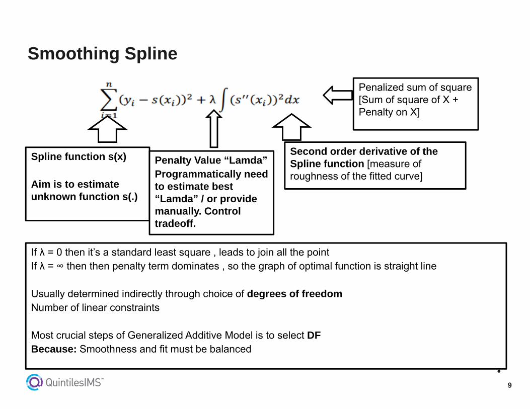
Smoothing Spline

Penalized sum of square [Sum of square of X + Penalty on X]

•

Spline function s(x)

Aim is to estimate unknown function s(.)

Second order derivative of the Spline function [measure of roughness of the fitted curve]

Penalty Value “Lamda”Programmatically need to estimate best “Lamda” / or provide manually. Control tradeoff.

If λ = 0 then it’s a standard least square , leads to join all the point If λ = ∞ then then penalty term dominates , so the graph of optimal function is straight line

Usually determined indirectly through choice of degrees of freedom Number of linear constraints

Most crucial steps of Generalized Additive Model is to select DFBecause: Smoothness and fit must be balanced

10

Characteristics of “Lamda”

11

• Less smoothing Less Bias Large Noise

Optimal “Lamda”

Noise prediction: Each of our predictions are going to be an average over just few observation (Irreducible error)

Smoothing less means large varianceTotal Error = (Noise)+(Bias)^2+(variance)Changing the amount of smooth has opposite effects on the BIAS and variance.Error due to BIAS: The error due to bias is taken as the difference between the expected (or average) prediction of our model and the correct value which we are trying to predict.

Error due to Variance: The error due to variance is taken as the variability of a model prediction for a given data point.

12

• To find the Optimal amount of smoothing …

Optimal “Lamda” and how to find it..

Cross Validation: Spline fit without the (Xi, Yi) point

This allow us to find “Lamda” for a given spline basis that minimizes this value, while taking the prediction of new points into account and avoiding danger of over-fitting.

“LEAVE ONE OUT” STRATEGY

As above equation is very computationally intense

Akaike’s Information Criterion (AIC) , Corrected AIC (AICC), Generalized cross Validation (GCV) (Matrix approach)

1. Leave One observation out2. Estimate smoothing curve using n-1 remaining observation3. Predict the value at the omitted point Xi4. Compare the predicted value at Xi with the real value Yi5. The difference between the original and predicted value at Xi 6. Repeat the process 7. Adding up all squared residuals give cross validation error

13

Plot

14

• Cubic Regression Spline (Special case of polynomial .. Third order)

Which Spline

degree 5degree 10

• Third order polynomials

• Computationally very efficient

15

• Thin Plate Regression Splines (default) PROC GAMPL

Which Spline..

• Works well, lend to slightly more linear than cubic spline

• Computationally more costly to set up

• Recommended to use polynomial spline in case of huge data

B spline, natural spline, P spline are also present.

16

GLM:

GAM

ppi xxxyg 22110)(

GAMs

)()()()( 210 pi xsxsxsyg

Smoothing function of Xi

17

Observational studies have suggested that low dietary intake or low plasma concentrations of Beta-carotene, or other carotenoids might be associated with increased risk of developing certain types of cancer.

A cross-sectional study , which want to investigate the relationship between personal characteristics and dietary factors, and plasma concentrations of Beta-carotene

Study subjects (N = 314) were patients who had an elective surgical procedure during a three-year period to biopsy or remove a lesion of the lung, colon, breast, skin, ovary or uterus that was found to be non-cancerous.

Aim is to identify factors which influence plasma concentrations of Beta-carotene

Case study: PROC GAMPL

18

plasma concentrations of Beta-carotene (Response)

Independent variables: (Continuous)

Age (Years)

QUETELET (weight/Height^2)

FIBER (Grams consumed/Day)

ALCOHOL (Number of alcoholic drinks consumed per week)

CHOLESTEROL consumed (mg per day)

BETADIET: Dietary beta-carotene consumed (mcg per day)

Independent variables: (Categorical)

Sex (1=Male, 2=Female).

Smoking status (1=Never, 2=Former, 3=Current Smoker)

Vitamin Use (1=Yes, fairly often, 2=Yes, not often, 3=No)

Variable Description:

19

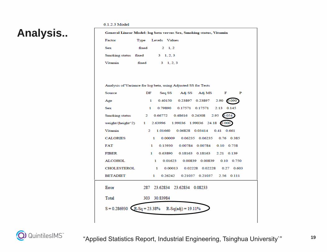
Analysis..

“Applied Statistics Report, Industrial Engineering, Tsinghua University`”

20

Check relation of Response and each dependent variables

proc sgplot data=Plasma;

scatter x=fiber y=betaplasma;

loess x=fiber y=betaplasma / nomarkers;

pbspline x=fiber y=betaplasma / nomarkers;

run;

Apply GAM – Diagnostics

21

ods graphics on;

proc gampl data=Plasma plots seed=12345;

class smokstat vituse ;

model betaplasma = spline(fiber) spline(betadiet) spline(quetelet) spline(age) param(smokstat) spline(cholesterol) param(vituse) spline(alcohol) / dist= GAUSSIAN;

id betaplasma;

output out=Predict;

run;

Apply GAM

Response distribution

22

Result and Output

23

•

Result and Output

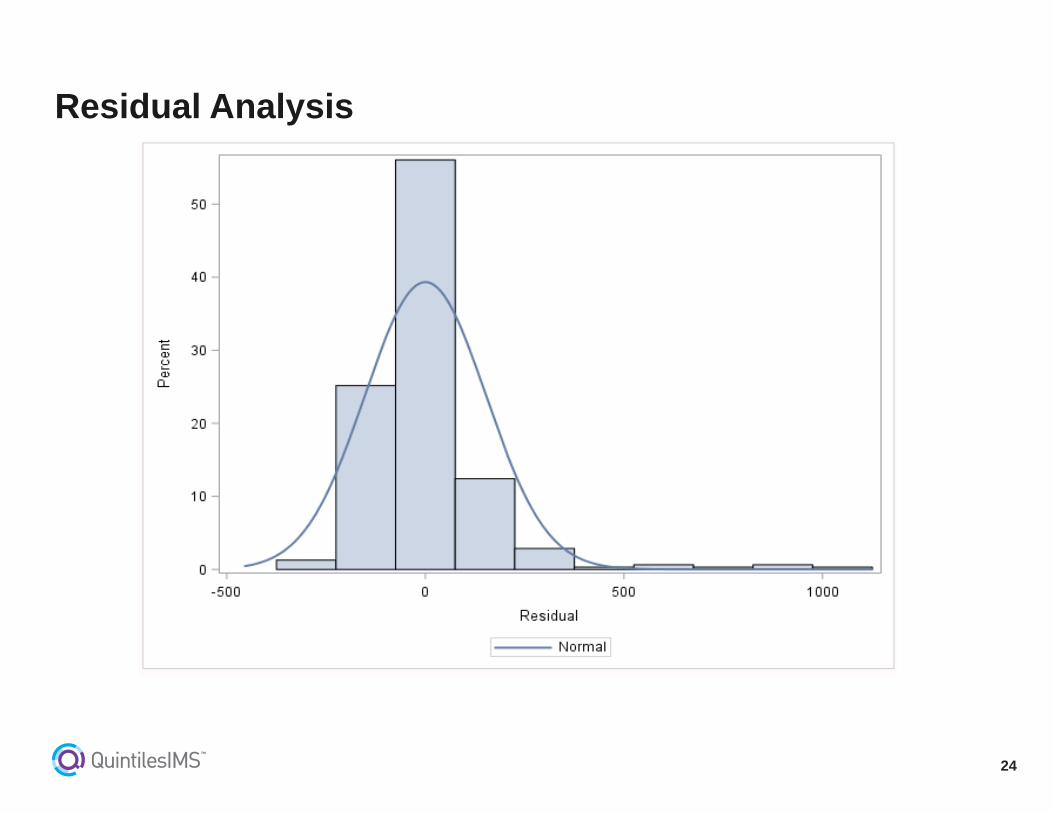
24

Residual Analysis

25

Transformation - LOG

26

Residual Analysis After Log transformation:

27

Can be use both liner and non linear exploratory variables in the model

When GLM fail to predict, GAM can be used

Summary

28

Discussion..

Thank you so much