Embed Size (px)
Citation preview

www.mtri.org
Mapping Submerged Aquatic Vegetation in the Great Lakes Using Satellite Imagery
Amanda Grimm, Robert Shuchman, Colin Brooks; Michigan Tech Research Institute (MTRI), Michigan
Tech University
October 2015, Acme, MI9th Biennial SoLM/15 th Annual GLBA Joint Conference
2
The Cladophora Problem
Cladophora is a native, filamentous, green alga that grows attached to solid substrate in all of the Laurentian Great Lakes (sparse in Lake Superior).
Becomes detached after significant storm events and washes up along shore, impairing recreational use of the lakes, clogging water intakes and facilitating avian botulism outbreaks.
Nuisance growth has become an increasing problem over the past decade despite reduced phosphorus loadings, due mostly to the arrival of invasive mussel species.
Mussel filtering is increasing water clarity, allowing Cladophora & other SAV to grow in deeper water.
Mussel “colonies” also create new areas of hard substrate where Cladophora can grow.

Mapping and Monitoring the Extent of Submerged Aquatic Vegetation in the Great Lakes
MTRI used Landsat satellite imagery to map the ca. 2010 extent of submerged aquatic vegetation in Lakes Michigan, Huron, Erie and Ontario.
Starting with raw Landsat imagery, a depth correction algorithm is used to eliminate radiance due to the water column, leaving just the radiance reflected from the lake bottom
By plotting multiple depth-corrected spectral bands (typically blue and green visible light) against one another, we can discriminate between bottom types (sand, mud, sparse and dense SAV)

Mapping and Monitoring the Extent of Submerged Aquatic Vegetation in the Great Lakes
Web-based, interactive GIS-style map established for all lake-wide SAV maps:
http://geodjango.mtri.org/static/sav/
(via http://www.mtri.org/cladophora.html)
5
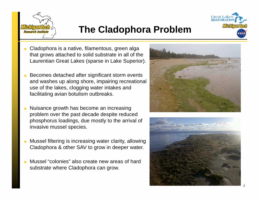
In Lake Michigan 28% of the visible bottom consisted of Submerged Aquatic Vegetation (SAV) (1220 km2 out of the 4390 km2 of visible bottom mapped)
MTRI’s nominal estimate of the dry weight biomass of the SAV in Lake Michigan is 67,000 metric tonnes.
30 m resolution map
Available at http://www.mtri.org/cladophora.html
Lake Michigan SAV/ Cladophora Map

Lake Michigan SAV/ Cladophora Map
6
Four main areas of concentrated SAV growth
Sleeping Bear Dunes
Green Bay
North end
Milwaukee
Apart from Milwaukee, these bloom areas are likely driven by nonpoint runoff rather than urban pollution
Mean satellite optical depth of 12 m (max >20 m)

MTRI’s bottom mapping procedure can also be used as an additional measure of water clarity
Northern Lake Michigan shows the greatest optical depth while southeast Lake Michigan shows the least.
Optical depth varies from 2 to 20+ meters
Optical depth can be used to estimate water clarity, photosynthetically active radiation, and photic zone
Mapping and Monitoring the Extent of Submerged Aquatic Vegetation in the Great
Lakes
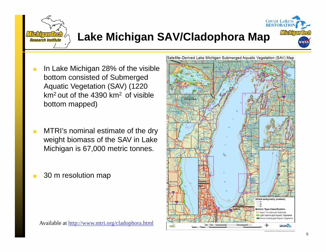
SAV Statistics by Lake
Total area mapped represents the geographic extent of optically shallow water that could be mapped with the Landsat sensor
Dry weight biomass estimates are derived from the mapped area of SAV and a nominal dry density of 50 g/m2 SAV
Estimates multiplied by 1.1 to account for SAV growing in optically deep water (based on the Great Lakes Cladophora Growth Model)
Basin-wide total of approximately 129,000 metric tonnes dry weight
8
Lake Total Lake Bottom Area Mapped by
Satellite (km 2)
Area Mapped as SAV (km 2)
Percent SAV of total area visible
Approx. SAV Dry Mass (metric tons)
Lake Michigan 4390 1220 28% 67,000
Lake Huron 4370 665 15% 36,000
Lake Erie 530 160 30% 9,000
Lake Ontario 790 315 40% 17,000
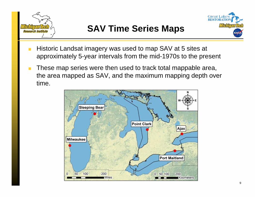
SAV Time Series Maps
Historic Landsat imagery was used to map SAV at 5 sites at approximately 5-year intervals from the mid-1970s to the present
These map series were then used to track total mappable area, the area mapped as SAV, and the maximum mapping depth over time.
9
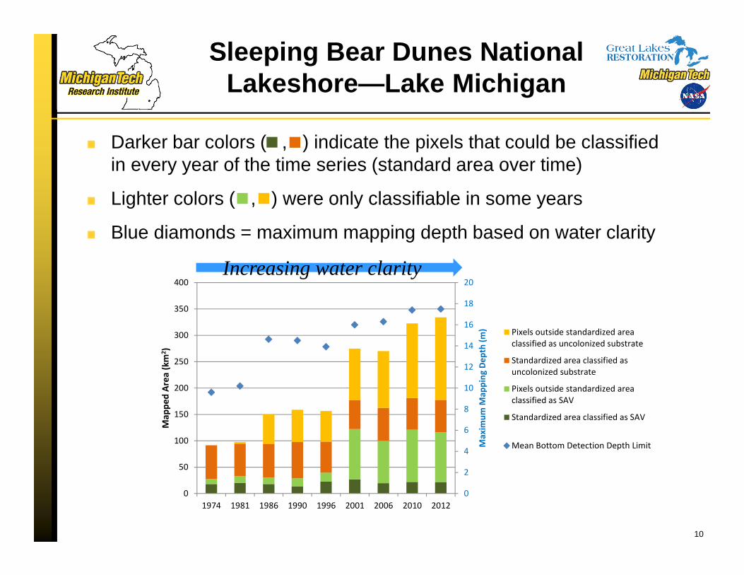
Darker bar colors ( , ) indicate the pixels that could be classified in every year of the time series (standard area over time)
Lighter colors ( , ) were only classifiable in some years
Blue diamonds = maximum mapping depth based on water clarity
Sleeping Bear Dunes National Lakeshore—Lake Michigan
10
0
2
4
6
8
10
12
14
16
18
20
0
50
100
150
200
250
300
350
400
1974 1981 1986 1990 1996 2001 2006 2010 2012
Ma
xim
um
Ma
pp
ing
De
pth
(m
)
Ma
pp
ed
Are
a (
km
2)
Pixels outside standardized area
classified as uncolonized substrate
Standardized area classified as
uncolonized substrate
Pixels outside standardized area
classified as SAV
Standardized area classified as SAV
Mean Bottom Detection Depth Limit
Increasing water clarity

Sleeping Bear Dunes National Lakeshore—Lake Michigan
Total area mapped as SAV at Sleeping Bear has increased nearly four-fold
Total mapped area increased more than three-fold due to higher water clarity
11
0
2
4
6
8
10
12
14
16
18
20
0
50
100
150
200
250
300
350
400
1974 1981 1986 1990 1996 2001 2006 2010 2012
Ma
xim
um
Ma
pp
ing
De
pth
(m
)
Ma
pp
ed
Are
a (
km
2)
Pixels outside standardized area
classified as uncolonized substrate
Standardized area classified as
uncolonized substrate
Pixels outside standardized area
classified as SAV
Standardized area classified as SAV
Mean Bottom Detection Depth Limit
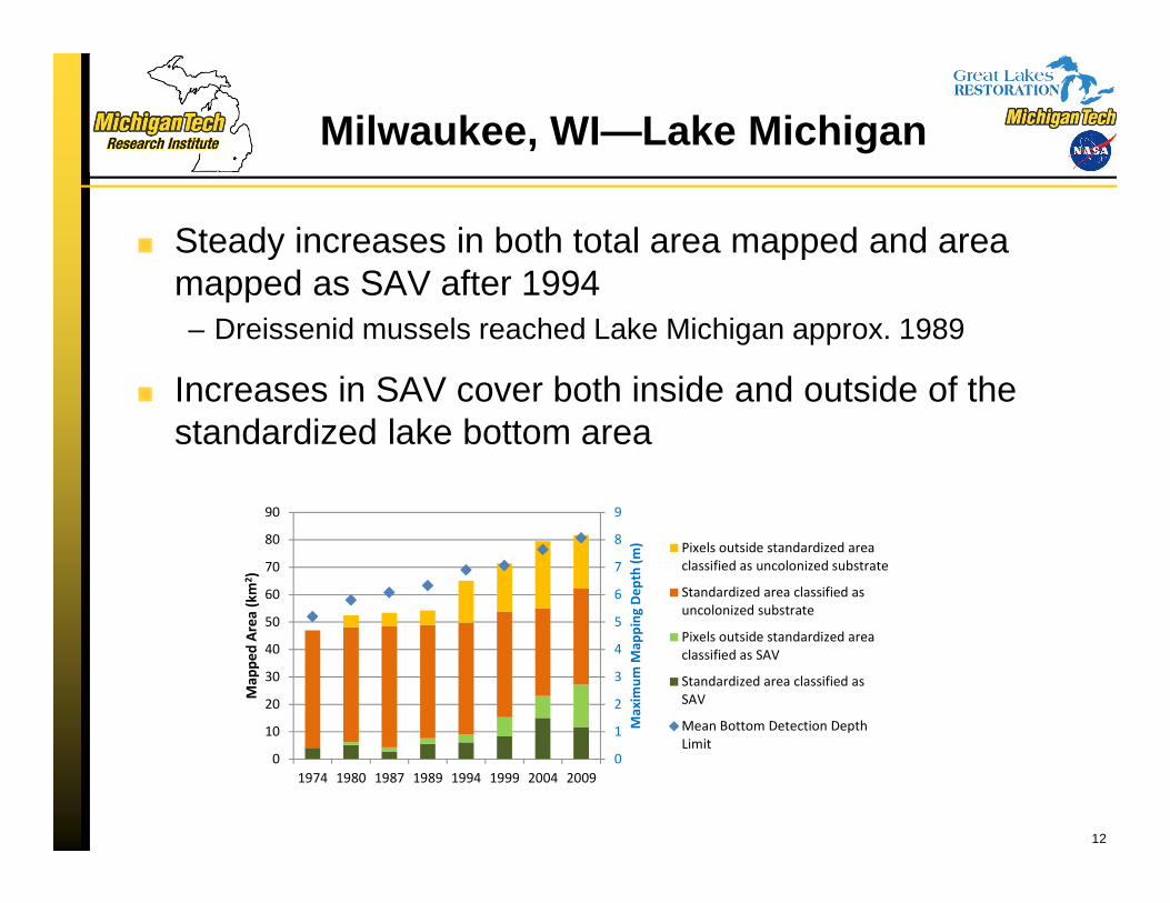
Milwaukee, WI—Lake Michigan
Steady increases in both total area mapped and area mapped as SAV after 1994– Dreissenid mussels reached Lake Michigan approx. 1989
Increases in SAV cover both inside and outside of the standardized lake bottom area
12
0
1
2
3
4
5
6
7
8
9
0
10
20
30
40
50
60
70
80
90
1974 1980 1987 1989 1994 1999 2004 2009
Ma
xim
um
Ma
pp
ing
De
pth
(m
)
Ma
pp
ed
Are
a (
km
2)
Pixels outside standardized area
classified as uncolonized substrate
Standardized area classified as
uncolonized substrate
Pixels outside standardized area
classified as SAV
Standardized area classified as
SAV
Mean Bottom Detection Depth
Limit
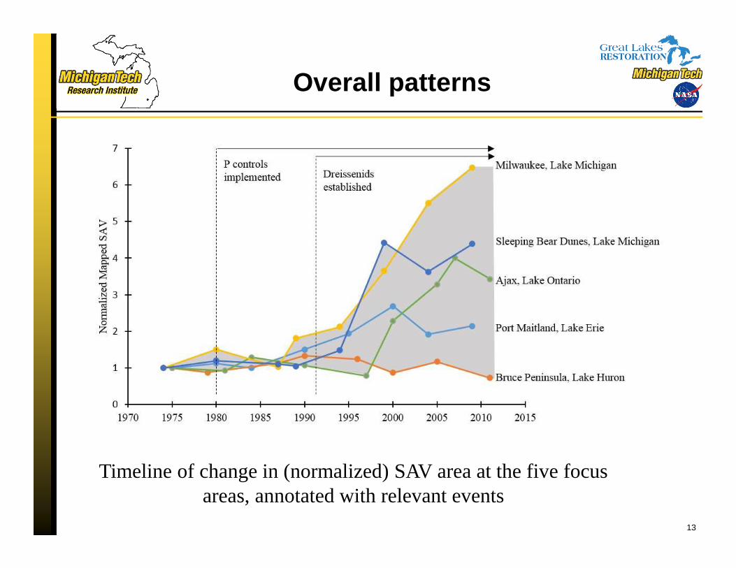
Overall patterns
13
Timeline of change in (normalized) SAV area at the five focus areas, annotated with relevant events
Overall patterns
Water clarity has increased significantly in all four lakes as a result of the activities of invasive dreissenid mussels
This increase in clarity is extending the area of suitable habitat for Cladophora and related vegetation into deeper water, leading to increases in total SAV area
Multiple sites exhibit a decline in SAV cover in the 1980s that coincides with phosphorus control efforts, then a resurgence following the date of appearance of dreissenid mussels at that particular site
14
Overall patterns
Many areas of especially concentrated SAV growth are clearly impacted by urban discharge (e.g. shorelines near Milwaukee, Toronto, Green Bay)
Others are not, for example, Sleeping Bear Dunes. Multiple possible nonexclusive explanations for these ‘hotspots’:– Current flow carrying nutrients to the site from more distant
inputs– Capture and recycling of allochthonous P by dreissenids– Increasing availability of hard substrate provided directly by
mussel beds forming on softer substrates
15

Recent Updates: Sleeping Bear
16
2012: 33% classified as SAV
Max mapping depth 18.2 m
2010: 34% classified as SAV
Max mapping depth 17.4 m
2013: 37% classified as SAV
Max mapping depth 20.1 m

Recent Updates: Western Shoreline
17
2010: 29% classified as SAV 2015: 40% classified as SAV
All of our time series work indicates significant changes at a ~5 year interval—time for a basin-wide update!
SAV/Cladophora GLRI Study: Concluding Remarks
Historic and current SAV cover varies along Great Lakes shorelines with ambient phosphorus levels, local nutrient sources, mussel density, water clarity, bottom substrate, and topography
The MTRI SAV algorithm provides robust estimates of SAV cover with an overall accuracy of ~83%
These basin-scale maps can help identify the priority watersheds for actions to reduce phosphorus loadings into the Great Lakes
The baseline map is now 5 years old – an update is needed to reflect recent changes and take advantage of the new Landsat 8 sensor
18Funded through EPA GLRI & NASA ROSES
Questions?
19
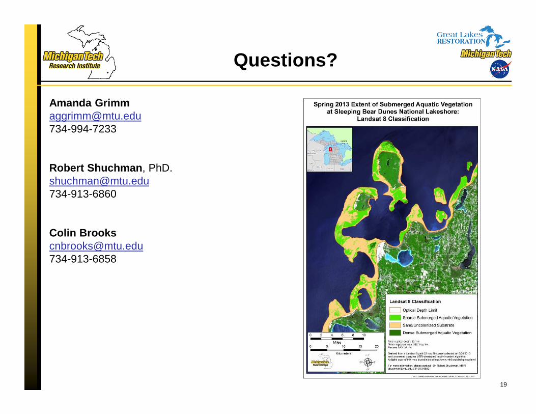
Amanda [email protected]
Robert Shuchman , PhD. [email protected]
Colin [email protected]