Glacier changes in southeast Alaska and northwest British ... · Glacier changes in southeast Alaska and northwest British Columbia and contribution to sea level rise Christopher

Glacier changes in southeast Alaska and northwest British

Columbia and contribution to sea level rise

Christopher F. Larsen,1 Roman J. Motyka,1 Anthony A. Arendt,1 Keith A. Echelmeyer,1

and Paul E. Geissler2

Received 1 June 2006; revised 21 August 2006; accepted 21 September 2006; published 24 February 2007.

[1] The digital elevation model (DEM) from the 2000 Shuttle Radar Topography Mission(SRTM) was differenced from a composite DEM based on air photos dating from 1948 to1987 to determine glacier volume changes in southeast Alaska and adjoining Canada.SRTM accuracy was assessed at ±5 m through comparison with airborne laser altimetryand control locations measured with GPS. Glacier surface elevations lowered over 95% ofthe 14,580 km2 glacier-covered area analyzed, with some glaciers thinning as much as640 m. A combination of factors have contributed to this wastage, including calvingretreats of tidewater and lacustrine glaciers and climate change. Many glaciers in thisregion are particularly sensitive to climate change, as they have large areas at lowelevations. However, several tidewater glaciers that had historically undergone calvingretreats are now expanding and appear to be in the advancing stage of the tidewater glaciercycle. The net average rate of ice loss is estimated at 16.7 ± 4.4 km3/yr, equivalent to aglobal sea level rise contribution of 0.04 ± 0.01 mm/yr.

Citation: Larsen, C. F., R. J. Motyka, A. A. Arendt, K. A. Echelmeyer, and P. E. Geissler (2007), Glacier changes in southeast Alaskaand northwest British Columbia and contribution to sea level rise, J. Geophys. Res., 112, F01007, doi:10.1029/2006JF000586.

1. Introduction

[2] Recent studies have documented that the majority ofalpine glaciers world-wide have been losing mass during thepast century and have been contributing to global sea levelrise [e.g., Dyurgerov and Meier, 1997; Arendt et al., 2002;Rignot et al., 2003; Paul et al., 2004; Dyurgerov andMcCabe, 2006]. Although temperate alpine glaciers repre-sent a small fraction of the world’s ice mass they arecontributing significantly to sea level rise through masswastage. Arendt et al. [2002] showed from analysis ofsmall-aircraft laser altimeter data that ice masses in Alaskaand neighboring Canada are thinning so rapidly that theymade a larger contribution to global sea level rise than theGreenland Icesheet during the later half of the 20th century.Nowhere in Alaska have these effects been more dramaticthan along the southern coastal mountains, where highannual accumulation rates (up to 4 m/yr water equivalent(weq)) and severe annual ablation (up to !14 m/yr weq)[Pelto and Miller, 1990; Eisen et al., 2001; Motyka et al.,2002] result in extremely high rates of ice mass exchange.[3] Most glaciers along the Gulf of Alaska have been

retreating since achieving their Little Ice Age (LIA)maximums sometime between 1750 and 1900 AD, in somecases quite rapidly [Goodwin, 1988; Mann and Ugolini,1985; Motyka and Beget, 1996; Calkin et al., 2001; Larsen

et al., 2005]. In this paper we examine glacier changes thathave occurred in southeast Alaska and adjoining Canadaduring the last half of the 20th century by comparing adigital elevation model (DEM) derived from the C bandNASA Shuttle Radar Topography Mission (SRTM) flown11–22 February 2000 to a DEM from the U.S. GeologicalSurvey National Elevation Dataset (NED) combined withthe Terrain Resource Information Management Program(TRIM) DEM from Natural Resources Canada.[4] Our study area includes 14,580 km2 of glaciers,

extending from 55!N, just south of the Stikine Ice Field(the southernmost major ice field that spans the borderbetween southeast Alaska and northwest British Columbia),to 60!N, the approximate limit of SRTM coverage (Figure 1).With a few exceptions, the NED is based on maps that wereproduced from 1948 aerial photography (Figure 2), and thusthe comparison for southeast Alaska generally documents52 yrs of ice elevation change. Coverage in Canada uses theBritish Columbia TRIM DEM derived from 1982 and 1987photography. The difference in the dates of the originalaerial photography is problematic, as glacial wastage in thisregion has been shown to be generally accelerating over thelatter half of the 20th century [Arendt et al., 2002]. How-ever, our DEM comparison offers a significant advance inareal coverage over previous glacial change studies here,and we show that the variation of surface elevation changesbetween various individual glaciers is far greater than thefactor of 2 increase in the rate of glacial wastage during thelatter part of the 20th century [Arendt et al., 2002]. Ourintent in this study is to focus on the spatial rather thantemporal variations in regional glacier change and thecontribution of these changes to sea level rise, and to

JOURNAL OF GEOPHYSICAL RESEARCH, VOL. 112, F01007, doi:10.1029/2006JF000586, 2007ClickHere

for

FullArticle

1Geophysical Institute, University of Alaska Fairbanks, Fairbanks,Alaska, USA.

2U. S. Geological Survey, Flagstaff, Arizona, USA.

Copyright 2007 by the American Geophysical Union.0148-0227/07/2006JF000586$09.00

F01007 1 of 11

http://dx.doi.org/10.1029/2006JF000586

explore what might be causing these dramatic and variedchanges.[5] Glaciers in our study area are temperate alpine and

predominately maritime that receive abundant precipita-tion: 7 m/yr to 1.5 m/yr weq with a strong inland gradient(http://www.wrcc.dri.edu/pcpn/ak.gif). Many glaciers insoutheast Alaska are now or have recently been tidewaterglaciers that calve icebergs and discharge meltwater directlyinto the sea. Numerous others calve into large proglaciallakes. The main goal of this study is to characterize the iceelevation changes exhibited over this large array of glaciers.Although laser altimetry elevation data are more accurate(±0.3 m), logistical costs prevent complete coverage of allglaciers within a given region, requiring extrapolation ofelevation changes to the entire region. Detailed annual massbalance measurements exist for only three glaciers in ourregion and are either of short duration, of uneven quality orboth [Pelto and Miller, 1990; Eisen et al., 2001;Motyka et al.,2002]. The spatial coverage afforded by differencing twoDEMs allows us to map a surprising variety of glacial changeswithin our study area. In addition, the method of comparingDEMs has advantages over altimetry and conventional massbalance for estimates of volume contribution to sea level risebecause it eliminates the problem of extrapolating from a fewknown to a large number of unknown glaciers.

2. Methods

[6] We obtained the SRTM and NED DEM for our studyregion from the USGS web server (http://seamless.usgs.gov), and the Canadian TRIM DEM from Geobase (http://www.geobase.ca). The NED DEM for the majority of ourregion is based on 1948 photography, and the CanadianDEM is based on 1982 photography south of 59 N, and1987 photography north of 59 N. Thus our comparisongenerally documents elevation change between 1948 and2000 in southeast Alaska, and between 1982/1987 and 2000in Canada (Figure 2).

[7] However, there are a few noteworthy exceptions(Figure 2). The NED photo base for most of the northernhalf of the Stikine Ice Field (which includes the tidewaterglaciers Dawes, South Sawyer, and Sawyer) (Figure 3)is from August 1961. A portion of the Yakutat Glacier(Figure 3) has photos from 1972. Hypsometry for severalglaciers in northeast Glacier Bay, includingMuir, Burroughs,and Carroll glaciers (Figure 3), was revised based on airphotos from August 1972. Similarly, part of the lower TakuGlacier (Figure 3) hypsometry was adjusted based on itsterminus position in 1971 air photos. These revised mapsfor northeast Glacier Bay and the Taku Glacier are the basisfor those portions of the NED DEM. We were able to obtainthe original contour maps based on 1948 photographs forboth the Taku glacier and northeast Glacier Bay. Wedigitized glacier contours on these 1948 maps and thenmodified the NED DEM using these data, so as to betternormalize the time span between DEMs in these areas.Similarly dated historic maps are not available for thoseportions of the Stikine Ice Field and the Yakutat Glacierhighlighted in Figure 2, and we were unable to normalizethe time span between DEMs there.[8] The SRTM DEM is available both in 30 m and 90 m

spacing. We used the 90 m spacing because we found thatboth resolutions provided similar results for our largeregional coverage. To ascertain vertical precision and anyvertical frame bias, we compared surface elevations over5 airfields (Figure 1) with elevations determined usingprecision GPS. Airfields were chosen because (1) they arelarge flat areas, so a large number of DEM grid cells can becompared with the GPS elevations and (2) they are non-vegetated, which is important because SRTM data oftengives elevations to the top of the forest canopy, which canbe 30–50 m high in southeast Alaska. This comparisonindicated no vertical frame bias, and standard deviation ofthe elevation difference on the airfields is 5 m (i.e., themean difference between GPS and SRTM on the airfields is0 ± 5 m).

Figure 1. Location map. Glaciers are shown in blue,covering a total of 14,580 km2. The four main glacierregions are shown by the dashed outlines (Yakutat, GlacierBay, Juneau and Stikine Ice Fields). Airports and altimetryprofiles used as ground control points for the SRTM DEMare shown in red.

Figure 2. Dates of air photos used to construct the topomaps that formed the earlier DEM.

F01007 LARSEN ET AL.: GLACIER CHANGES IN SOUTHEAST ALASKA

2 of 11

F01007

[9] The NED DEM for Alaska has a grid spacing of 45 mand was derived by digitizing the original contour maps.These maps have inaccuracies related to a variety of factors[see Arendt et al., 2002, supporting material (SM)]. Thenominal random error in elevation is 15 m or one half of thecontour interval. However, these uncertainties can be greaterat higher elevations and especially in glacier accumulationzones where featureless snow cover can make stereo per-ception and photogrammetric mapping difficult, and 30 to45 m errors are possible [Adalgeirsdottir et al., 1998;Arendt et al., 2002]. We follow these prior assessments ofelevation error in Alaskan USGS maps with the assumptionthat no additional error is introduced in digitizing thesemaps.[10] Before differencing, the NED was transformed from

the Alaska NAD27 horizontal datum to WGS84, the hori-zontal datum used in the SRTM. The vertical datums alsodiffer: the SRTM vertical datum is EGM96, while in Alaskathe NED is NGVD29. This is problematic, as no standardexists to transform NGVD29 heights in Alaska to any otherdatum. Indeed, the National Geodetic Survey (NGS)describes the NGVD29 as neither mean sea level, the geoid,nor any other equipotential surface. To estimate the offsetbetween these vertical datums, we found NGS benchmarkdescriptions with elevations published in both datums, andused a constant, average difference found at tidal bench-marks in Juneau, Haines and Skagway. To test the accuracyof this estimate, we again used the 5 airfields (Figure 1), thistime as locations where the elevations of a large number ofpixels from both DEMs were directly compared. Bothassessments find the NGVD29 to be lower than theEGM96 by 2.3 ± 0.6 m (1s).[11] The SRTM was interpolated to the same 45 m grid as

the transformed NED. Both the NED and Canadian DEMswere then subpixel registered to the SRTM using an image

warping program (the USGS Astrogeology Integrated Soft-ware for Imagers and Spectrometers, ISIS). This last step iscritically important as small offsets between the DEMs canlead to large errors in an elevation difference map [e.g.,Berthier et al., 2004]. The results of differencing the DEMswere then masked with outlines of the glacial cover. TheGlobal Land Ice Measurements from Space project (http://www.glims.org) has digitized a number of glacier outlinesin our study area using Landsat images [Beedle et al., 2006].We used Beedle et al.’s [2006] work as a base to redigitizeand extend outlines to meet our need for a complete glacieroutline database across our study area. We then adjustedthese outlines using USGS and Canadian contour maps tomore accurately reflect initial conditions in terminus regionswhere pronounced changes in ice-covered area haveoccurred at most glaciers. However, on the few advancingglaciers, the outlines were generated solely from newimagery to reflect the present ice-covered area. In general,the masking of the elevation difference map includes ice-covered area if ice was present at the time of either DEM.

3. Accuracy and Error Analysis

[12] To estimate accuracy of SRTM data over glaciers, wecompared SRTM data to light aircraft laser altimetry dataobtained in late August of 2000 at 12 glaciers distributedthroughout the study area (Figure 1). Vertical precision ofthe altimetry technique is "0.3 m with points spaced every"1.2 m along the centerline of each glacier [Echelmeyer etal., 1996; Adalgeirsdottir et al., 1998; Arendt et al., 2002].When comparing these data, the SRTM DEM was extrap-olated between grid cells with a bicubic interpolation.Approximately 5 # 104 laser altimeter derived elevationswere compared to the SRTM DEM (Figure 4). A lineartrend was fitted to the differenced data, and the standarddeviation about this trend indicates an overall accuracy ofthe SRTM data over glaciers to be slightly better than ±5 m(Figure 4b).[13] There are several reasons for elevation differences to

be correlated with elevation in the SRTM to laser compar-ison. The slope (2.6 m per 1000 m elevation) and offset(!2.5 m at zero elevation) of the trend with elevation iswhat one might expect from the seasonal difference betweenthe two measurements (late August 2000 for the altimetrymeasurements versus February 2000 for SRTM), associatedwith ablation, accumulation, densification, and ice flow.The contour maps that form the basis for the earlier DEMsfor southeast Alaska and adjoining Canada were derivedfrom aerial photography flown during late summer, soadjusting the SRTM to a late summer surface is desirablein order to examine nonseasonally affected changes insurface elevation. In addition to seasonal differences, theelevation difference trend is also partially caused by radarpenetration depth and its dependence on elevation [Rignot etal., 2001]. We take the linear trend shown in Figure 4 toaccount for both seasonal and radar penetration effects anduse it to adjust the SRTM DEM as a function of elevationprior to differencing with the earlier DEM.[14] Berthier et al. [2006] have found SRTM elevation

biases over non-glacier-covered terrain, but with a strongerdependence on elevation than we find. These biases may beintroduced in the processing of the SAR data used for the

Figure 3. Locations of specific glaciers named in text. Thecolor scheme is the same as in Figures 8 and 9, with greenfor tidewater glaciers, blue for lake calving glaciers, and redfor land terminating. Glacier cover not included in theglacier class analysis discussed in the results section yetdisplayed in Figures 8 and 9 is shown in white.


3 of 11

F01007

SRTM DEM and may increase more rapidly at higherelevations [Berthier et al., 2006; B. Rabus, personal com-munication, 2005]. The range of elevations over which wecompare SRTM and laser altimetry elevations is somewhatlower than the elevations used in the analysis of Berthier etal. [2006]. Furthermore, our only comparison over non-glacier-covered terrain of SRTM elevations to GPS derivedelevations is limited to near sea level at the 5 airfieldsshown in Figure 1.[15] We use 5 m as a measure of uncertainty of the SRTM

elevation data. For NED and Canadian DEMdata, we assumean uncertainty of ±15 m for elevations below the equilib-rium line altitude (ELA) (which averages about 1000 mfor our region) and ±30 m above the ELA. Altimetrycomparisons have suggested that individual sections of theoriginal contour maps may have systematic errors of up to!13 m in the Chugach Range and +45 m in the BrooksRange due to poor ground control or photogrammetricerrors, with a normal range on the order of ±2 m [Arendtet al., 2002, SM; Arendt et al., 2006, SM]. The uncertaintyin estimating the offset in vertical datums is ±0.6 m. Thefirst two errors are random in nature while the second twoare systematic, but overall the errors associated withcontour maps dominate. Standard propagation of therandom errors leads to a combined per pixel 1s uncer-tainty in elevation change from our DEM comparisons of±16 m at lower elevations and ±30 m at higher elevations,with an additional 2.6 m systematic error possible. For rateof elevation change, uncertainty values at low and highelevations are ±0.3 m/yr and ±0.6/yr for 1948–2000 (mostof southeast Alaska), ±0.4 m/yr and ±0.8/yr for 1961–2000 (parts of the Stikine Ice Field in Alaska), ±0.9 m/yrand ±1.6 m/yr for 1982–2000 (BC, south of 59 N), and±1.2 m/yr and ±2.3 m/yr for 1987–2000 (BC, north of 59 N).[16] To test the uncertainties estimated above, we

differenced the two DEMs over non-ice-covered areas.The mean of the off-ice difference map is zero, suggestingthat our transformation between vertical datums prior todifferencing the DEMs was correct. However, the median isslightly positive and, indeed, the distribution of non-iceelevation differences is strongly non-Gaussian (Figure 5).This is problematic, as the use of standard deviation (SD) asan estimate of the spread of the data is now not valid. Weinstead use the interquartile range (IQR) as an estimate ofthe errors associated with the DEM differencing. We find an

IQR of ±16.5 m over more than 1 # 108 pixels comparisons(representing over 200,000 km2 of non-ice-covered area).This error approximation is just slightly greater than theformal errors estimated above. When expressed in terms ofrate of elevation change errors, this IQR corresponds to±0.3 m/yr. Some minor dependence in the magnitude of thiserror estimate was found with elevation and slope. It shouldbe noted, however, that most of the higher elevations in ourdifference map are ice covered, and so an independent testof the errors associated with accumulation areas (asdiscussed above) is not feasible.[17] An additional source of error is the uncertainty in

mapping of ice covered area. Sensitivity tests in whichseveral different glacier outline databases were used involume calculations in the western Chugach Mountainsshow that volume change estimates there varied 10%

Figure 4. (a) Laser minus SRTM elevation difference versus elevation. (b) Distribution of laser minusSRTM elevation difference. The red curve is a Gaussian fit over the distribution, and the blue verticallines bracket the standard deviation (SD = ±5 m).

Figure 5. Distribution of DEM difference map values overnonglacier covered areas as used to estimate glacierelevation change errors. The red curve is a Gaussian overthe distribution, showing poor quality of fit. The standarddeviation (‘‘std,’’ bracketed by red lines) is 19.0 m, but amore robust estimate of the spread is shown by theinterquartile range (‘‘iqr,’’ bracketed by blue lines), whichis 16.5 m for this distribution.


4 of 11

F01007

between the various outlines used [Arendt et al., 2006]. Forthis study, we have only one glacier outline databaseavailable and so are not able to determine the errorsintroduced from glacier area uncertainties.

4. Results: Elevation and Volume Changes

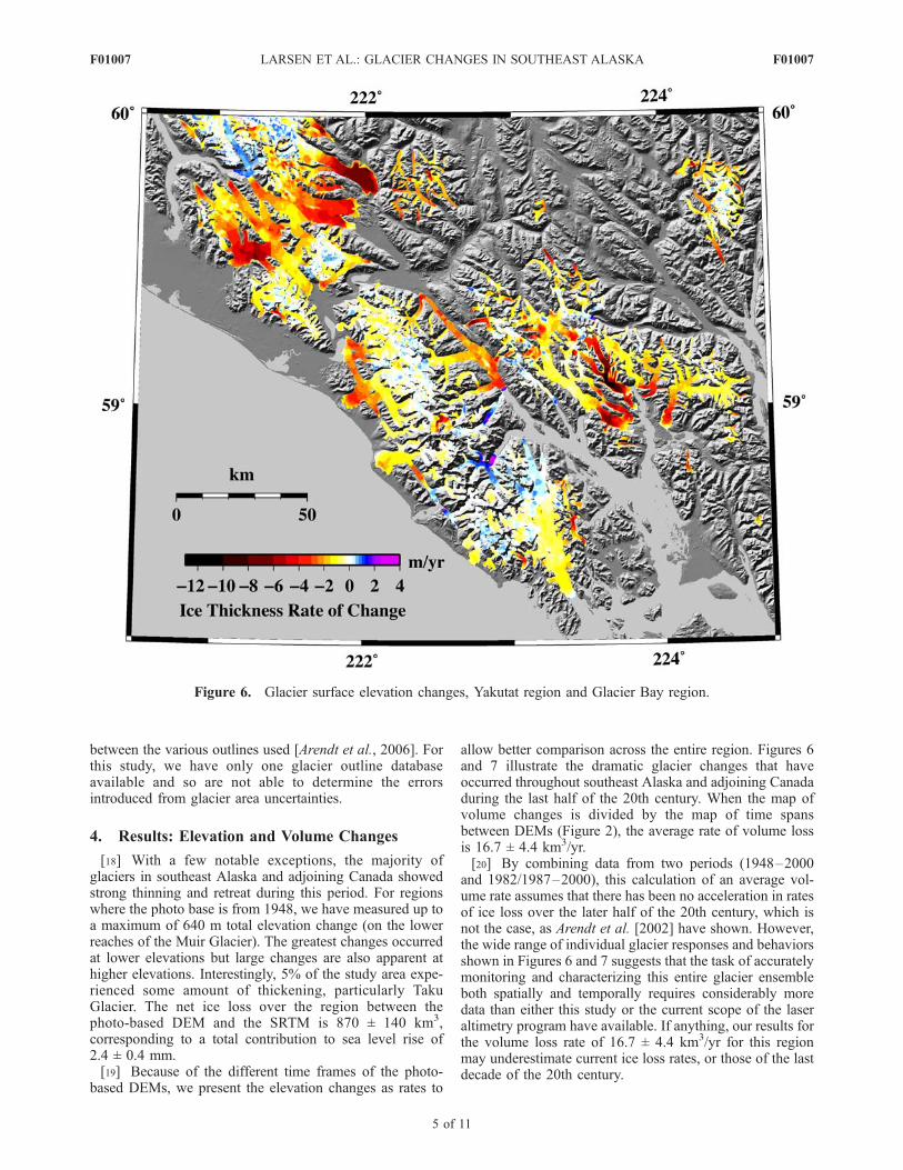
[18] With a few notable exceptions, the majority ofglaciers in southeast Alaska and adjoining Canada showedstrong thinning and retreat during this period. For regionswhere the photo base is from 1948, we have measured up toa maximum of 640 m total elevation change (on the lowerreaches of the Muir Glacier). The greatest changes occurredat lower elevations but large changes are also apparent athigher elevations. Interestingly, 5% of the study area expe-rienced some amount of thickening, particularly TakuGlacier. The net ice loss over the region between thephoto-based DEM and the SRTM is 870 ± 140 km3,corresponding to a total contribution to sea level rise of2.4 ± 0.4 mm.[19] Because of the different time frames of the photo-

based DEMs, we present the elevation changes as rates to

allow better comparison across the entire region. Figures 6and 7 illustrate the dramatic glacier changes that haveoccurred throughout southeast Alaska and adjoining Canadaduring the last half of the 20th century. When the map ofvolume changes is divided by the map of time spansbetween DEMs (Figure 2), the average rate of volume lossis 16.7 ± 4.4 km3/yr.[20] By combining data from two periods (1948–2000

and 1982/1987–2000), this calculation of an average vol-ume rate assumes that there has been no acceleration in ratesof ice loss over the later half of the 20th century, which isnot the case, as Arendt et al. [2002] have shown. However,the wide range of individual glacier responses and behaviorsshown in Figures 6 and 7 suggests that the task of accuratelymonitoring and characterizing this entire glacier ensembleboth spatially and temporally requires considerably moredata than either this study or the current scope of the laseraltimetry program have available. If anything, our results forthe volume loss rate of 16.7 ± 4.4 km3/yr for this regionmay underestimate current ice loss rates, or those of the lastdecade of the 20th century.

Figure 6. Glacier surface elevation changes, Yakutat region and Glacier Bay region.


5 of 11

F01007

[21] Most of the glacierized terrain in southeast Alaskaand adjoining Canada falls into four distinct regions:Yakutat, Glacier Bay, Juneau Ice Field, and Stikine IceField (Figure 1). Glaciers in our study area account forabout 17% of the total glacier area in Alaska and adjoiningCanada. This glacier-covered area is three times the area ofSwiss Alps glaciers and equal to the combined area ofthe Northern and Southern Patagonia Ice Fields. Thevolume changes documented here show that southeastAlaska and adjoining Canada contributed an average of0.04 ± 0.01 mm/yr to sea level rise during the later half ofthe 20th century, assuming all the volume lost is ice with adensity of 0.9 kg/m3. The rate of sea level rise contributionwe find from glaciers in southeast Alaska and adjoiningCanada is effectively equal to that from all Patagonia

glaciers during the period 1968/1975–2000 (0.042 mm/yr)[Rignot et al., 2003].[22] To obtain a rough estimate of the relative contribu-

tions to ice loss from different classes of glaciers weanalyzed ice volume changes on 74 individual glaciers:32 land terminating glaciers (covering 2054 km2), 20 tide-water glaciers (covering 4033 km2), and 22 lake calvingglaciers (covering 2870 km2). The total area analyzed byglacier class thus comprises about 62% of the region’s totalglacier covered area (Figure 3). Figure 8 shows the widevariations in area-averaged thinning rates on various indi-vidual glaciers from across our study region. The results ofthis analysis show that over two thirds of the losses arecoming from calving glaciers and that the losses from lakeglaciers are slightly greater than those from tidewater

Figure 7. Glacier surface elevation changes, (a) Juneau Ice Field and (b) Stikine Ice Field.


6 of 11

F01007

glaciers (Figure 9). Perhaps the most surprising result of thisanalysis is that lake calving glaciers are thinning faster perarea than the tidewater calving glaciers of southeast Alaska,and, in particular, one lake calving glacier (Yakutat) hasvery nearly the largest rate of volume loss of any glacier inthe region.

5. Discussion5.1. Climate Change

[23] Climate change is commonly invoked as a factorcausing the negative trend in global glacier mass balances.

The surface mass balance of glaciers is largely determinedby the magnitude of summer air temperatures, whichrepresents the variability in solar radiation and sensible heatavailable for melting, and winter snowfall, which deter-mines the net surface accumulation. Previous studies haveshown that annual air temperatures in Alaska have increasedduring the past 50 years, with winter increases approxi-mately double those occurring during the summer [Staffordet al., 2000]. Rasmussen and Conway [2003] suggest thesummer temperature increases were sufficient to explain thewidespread glacier mass loss in Alaska and northwesternCanada, but little work has been done to investigate thepotential effects of winter warming on the distribution andtype of winter precipitation in this region. Precipitation is animportant component of the mass balance in maritimeregions such as southeast Alaska, where accumulation ratesare as high as 4 m weq/yr [Eisen et al., 2001; Motyka et al.,2002; Pelto and Miller, 1990], compared to 1–2 m weq forAlaska interior continental glaciers [March, 2003; Mayo etal., 2004].[24] We obtained climate data from the National Climate

Data Center for 1948 to 2000 for weather stations located inour study area and calculated daily means of temperatureand precipitation for each season: annual, winter (Novemberto April), and summer (May to October). The long-termchanges in temperature and precipitation were calculatedwith a linear regression, and are shown in Table 1. Weassume that the climate trends do not vary with elevationand represent climate trends at the glaciers, while recogniz-ing that at times the local mountain conditions can varysubstantially from those occurring at low elevations. Meanannual air temperature measured at Juneau, Sitka, andYakutat increased from 1948 to 2000. Total precipitation(rain and snow) increased slightly at Juneau and Sitka but atYakutat, total precipitation increased by about 1.5 m/yr. Aslight increase in winter precipitation was observed at bothJuneau and Sitka and a much stronger increase in Yakutat.However, the 1.8!C increase in average winter temperaturewould likely have driven snow lines higher in altitude.[25] Because the vast majority of glacier covered area in

our study area is below 2200 m in elevation, the effect ofhigher temperatures probably dominates over increasedprecipitation, causing negative mass balance. For thoseglaciers with a substantial part of their accumulation areasat high elevation, increased precipitation would translateinto greater snowfall and these glaciers could benefit andthicken. For example, some high areas of the Fairweather

Figure 8. (top) Volume change rates versus area-averagedelevation. (bottom) Area-averaged thinning rates versusarea-averaged elevation.

Figure 9. (a) Total contributions by glacier type of the individual glaciers analyzed. (b) Same asFigure 9a, but with the advancing tidewater glaciers removed from the tidewater sum.


7 of 11

F01007

Range indicate surface elevation increases (Figure 6). How-ever, the results for these areas are especially subject to thegreater errors associated with photogrammetric mapping ofaccumulation zones, and may not be significant.

5.2. Glacier Hypsometry and ELA

[26] The above comparison between glacier and climatechanges assumes a static glacier surface geometry. In reality,the response of the volume of a glacier to climate iscomplicated because the changing surface configurationacts as a feedback which affects the response. Throughfeedback effects, glaciers usually attain a new equilibriumvolume through terminus retreat, reducing the amount ofarea at low elevations where balances are most negative. Anopposite, destabilizing effect occurs as the glacier surfaceelevation decreases. However this effect is usually second-ary to those occurring due to terminus changes. The time-scales over which these dynamic adjustments occur are onthe order of decades, so that the volume changes of a glacierrepresent the integrated effects of climate during and beforethe period of measurement [Elsberg et al., 2001]. Thereforewe note that our discussion in the previous section is a first-order approximation of the effects of climate on glacierchanges.[27] Glacier surface geometry also plays a role in deter-

mining the sensitivity of glaciers to climatic changes. Theequilibrium line altitude (ELA) separates the accumulationand ablation zones on a glacier, and its fluctuations relativeto the glacier hypsometry determine the glacier sensitivity toclimate change. For example, a glacier with broad, flat areasnear the long-term ELAwould be more sensitive to climaticfluctuations than one with little area near the ELA. We foundthe regional average ELA was between 900 to 1100 m,based on an analysis of the change in inflection of contourson the topographic maps [Leonard and Fountain, 2003],and an examination of available mass balance data. Assum-ing a summer temperature increase of 0.8!C, the ELAwouldincrease by 100 m, if precipitation and radiation balanceremained constant [Hooke, 1998]. Except for glaciers flow-ing from the Fairweather Range (which rise to 4600 m),glaciers in our study region drain mainly from relatively lowmountain ranges (<2200 m) and have accumulation areasthat predominately lie below 1800 m in elevation. TheBrady and Yakutat Glaciers are particularly sensitive tochanges in climate because their accumulation areas arenear or even below the long-term ELA (Figures 3 and 6).The ice field that contains the Yakutat Glacier, which islosing ice at rates of up to 8 m/yr, mostly lies below 1000 mand has essentially lost its accumulation area. This ice fieldwill likely disappear completely under current conditions.Thinning rates on the Brady Ice Field, which lies mostly

below 1200 m, are also losing mass at a rate which is abovethe regional average (2 to 3 m/yr).

5.3. Glacier Dynamics

5.3.1. Tidewater Glaciers[28] Some of the largest ice losses in southeast Alaska are

occurring at tidewater glaciers that are known to haveundergone calving retreats during all or part of the timeperiods covered in this study, e.g., LeConte, South Sawyer,Dawes, and Muir Glaciers (Figures 3, 6, and 7). Theseglaciers have experienced up to 640 m of thinning in theirterminal reaches (Muir) and 100 m or more at higherelevations. Tidewater glaciers become unstable when theterminus retreats from its protective shoal into a deep basinand rapid calving ensues [Post, 1975]. Although the retreatmay be triggered by climate (or other factors), these calvingretreats become independent of climate as described in the‘‘tidewater glacier cycle’’ [Meier and Post, 1987; Post andMotyka, 1995]. Once begun, the retreat phase of this cycle issubject to increasing positive feedbacks as surface slopesand flow velocities substantially increase at the terminusand throughout the length of such glaciers, causing signif-icant drawdown of the parent ice field and further increasingcalving flux [Pfeffer et al., 2000; O’Neel et al., 2001]. Thisphase of the tidewater cycle has been observed to lead toterminus retreat in excess of 1 km/yr in southeast Alaska.Surface mass balance data on tidewater glacier is sparse, butinterpolation of available data indicates that for retreatingtidewater glaciers calving is by far the dominant mode of iceloss (>90%) [Brown et al., 1982; O’Neel et al., 2003].Because of the magnitude of ice loss relative to noncalvingglaciers is so large, retreating tidewater glaciers tend to bethe dominate contributor to sea level rise in coastal Alaska[cf. Arendt et al., 2006]. The importance of this assertion isthat a significant proportion of current ice loss in southeastAlaska is due to the dynamics of tidewater glaciers and notdirectly forced by climate change, aside from the initiationof the calving retreats.[29] In contrast to widespread glacier wastage and retreat

in southeast Alaska and adjoining Canada, seven glaciers inthe region are growing. Taku Glacier, which drains from theJuneau Ice Field (Figure 7), is the most notable, havingadvanced over 7 km since 1890. Surface elevations haveincreased over 200 m in its terminus area and over 100 m athigher elevations since 1948 [Motyka and Echelmeyer,2003]. Causes of the Taku Glacier advance have beenaddressed in several articles [Motyka and Beget, 1996; Postand Motyka, 1995; Nolan et al., 1996] and are primarilyrelated to the advance phase of the tidewater glacier cycle[Post and Motyka, 1995]. Briefly, when a tidewater glaciersuffers a large calving retreat most of its ablation area is lost.This leads to positive imbalance, and the glacier respondswith advance and growth [Post, 1975]. The terminus ofTaku Glacier has now emerged above tidewater and it nolonger calves. Other glaciers that were in advance phase ofthe tidewater glacier cycle in between the dates of the twoDEMs analyzed here include Johns Hopkins, Reid, andLampaugh in Glacier Bay, and North Crillon in Lituya Bay,which all continue to calve, and Lituya Glacier in LituyaBay and Art Lewis Glacier in Nunatak Fiord, which are nowgrounded above sea level (Figure 6). Even for stable andadvancing tidewater glaciers, calving can often be the

Table 1. Temperature and Precipitation Change, 1948–2000:Annual, Winter, and Summera

Location

Temperature, !C Precipitation, mm

Summer Winter Annual Summer Winter Annual

Juneau 1.0 1.6 1.5 81 141 223Sitka 0.5 1.8 1.1 44 95 163Yakutat 0.8 1.9 1.3 811 646 1528

aWinter is November–April, and summer is May–October.


8 of 11

F01007

dominant mode of annual ice loss [Brown et al., 1982;Trabant et al., 1991].5.3.2. Lake-Terminating Glaciers[30] Many lacustrine glacier systems have also experi-

enced significant ice losses in southeast Alaska, e.g., amongthe largest are Yakutat, Grand Plateau, and Alsek glaciers,whose lower reaches have thinned by 200 to 350 m(Figures 3 and 6). These three glaciers all calve icebergsinto large lakes that formed as the glaciers retreated fromtheir LIA terminal moraines into overdeepened basins. Infact, many proglacial lakes of all sizes have formed through-out the region as a result of retreat, often during the periodcovered by this study, and the development of these lakesthus introduces a calving component into the balance equa-tion of these glaciers [Viens, 2001]. Unfortunately, except forMendenhall Glacier, data on calving speeds and surfacemass balance on lake calving glaciers in our study area arevirtually nonexistent. Thus it is difficult to assess the relativeimportance of calving dynamics in overall ice loss for lake-terminating glaciers. Although studies have shown thatcalving rates for lake-terminating glaciers tend to be muchlower than for their tidewater calving cousins for equivalentdepths (see van der Veen [2002] for a review), calving lossescan apparently still play a significant roll in glacier massbalance for some deep water lake terminating glaciers inPatagonia [Venteris, 1999; Warren and Aniya, 1999]. At theother extreme, calving losses at Mendenhall Glacier, a smallvalley glacier near Juneau, account for only 4% of the totalice losses although calving has been an important agent ofglacier retreat [Motyka et al., 2002; Boyce et al., 2007]. Incontrast to tidewater glaciers, only one lake-terminatingglacier is known to be currently advancing in southeastAlaska. South Crillion Glacier, located just south of LituyaBay in the Fairweather range, is advancing into CrillionLake. However, South Crillion’s advance is probably drivenby the larger-scale tidewater dynamics of North CrillionGlacier, to which South Crillion is joined.5.3.3. Surging Glaciers[31] Glacier surges constitute another flow instability that

can contribute to glacier changes (see Raymond [1987] andHarrison and Post [2003] for reviews) and we attribute thestrong thinning observed in the terminus region of Tweeds-muir Glacier (Figures 3 and 6) to the aftermath of a surge in1973.5.3.4. Stranded Glaciers[32] A subsidiary effect of calving glacier retreat is that

tributary glaciers can become stranded by the retreat of themain trunk glacier and drawdown of the parent ice field.Glacier Bay, which is now surrounded by numerous discreteglaciers and small isolated ice fields, contained a hugecontinuous ice field with ice up to 1.5 km thick that coveredmore than 6000 km2 as recently as 250 years ago [Larsen etal., 2005]. The 120 km retreat and collapse of the parentLIA ice field between 1750 and 1929 AD stranded manytributary glaciers. Some were entirely isolated from anysource of accumulation and are now simply wasting away(e.g., Burroughs Glacier). Other glaciers have had theiraccumulation areas substantially reduced as the ice fieldsfeeding the LIA tidewater glaciers disappeared and are nowsusceptible to the effects described earlier as a consequenceof hypsometry and rising ELA. The strong ice lossesexhibited at Yakutat, Novatak and Nunatak Glaciers may

in part be attributable to the demise of Nunatak Glacierduring the 19th century [Barclay et al., 2001]. Post-LIAretreats in Tracy Arm, Endicott Arm, and LeConte Bay alsocontributed to isolation and wastage of several tributaryglaciers.

5.4. Comparison of Losses to Laser AltimetryEstimates

[33] Arendt et al. [2002] compared small aircraft laseraltimetry profiles acquired over 70 glaciers in Alaska andneighboring Canada to elevations from USGS and Canadiantopographic maps. Results of the analysis were extrapolatedto nonprofiled glaciers to estimate losses from all ice-covered areas in NW North America. Twelve glaciers wereprofiled in southeast Alaska at the time of the study. Wecompared our results to the results from this earlier extrap-olation and found that area-averaged thinning rates forsoutheast Alaska in the earlier study may have been under-estimated by more than a factor of two (Figure 10). Weattribute this discrepancy to two factors: (1) the smallnumber of profiled glaciers and (2) tidewater and lakecalving glaciers were underrepresented in southeast Alaskaat the time of 2002 study. Although the time period coveredby our analysis does include both the ‘‘early’’ ("1950 to"1995) and ‘‘recent’’ ("1995–2001) periods discussed byArendt et al. [2002], and therefore should include someeffect of the accelerated wastage of the recent period, thiseffect is not enough to account for a factor of two differencein thinning rates averaged over the whole period.[34] Arendt et al. [2002] specifically removed tidewater

glacier data from the composite profiles used in theirextrapolation of measured rates of surface elevation change.The reasoning behind this choice is clear: one would notwant to extrapolate thinning rates from rapidly disintegrat-ing tidewater glaciers to the remaining ice coverage in a

Figure 10. Comparison of DEM differencing results andlaser profiling. The solid black line shows the rate ofelevation change averaged in 10 m elevation bins across allof the glacier covered area analyzed here. The dashed graylaser profile curve is what was used to extrapolate from thefew profiled glaciers in southeast Alaska to the remainingunprofiled glacier area [Arendt et al., 2002].


9 of 11

F01007

region. However, by extrapolating thinning rates from non-tidewater glaciers to a region which does indeed have asignificant percentage of tidewater (and lacustriane) glacierarea, Arendt et al. [2002] implicitly assumed that theseunmeasured calving glaciers were not making an aboveaverage contribution, individually, to the regional volumeloss. In the absence of data from the calving glaciers in aregion, this method of extrapolation is the only practicalapproach. That it appears to have underestimated thevolume loss in our study area by more than a factor oftwo strongly emphasizes the need for greatly expanded laseraltimetry over as many glaciers as possible in order toobtain an accurate assessment of glacier change. Repeatedprofiling of glaciers strongly affected by glacier dynamicsthat may be contributing disproportionately to ice loss,particularly calving glaciers, is critically important to deter-mine present volume rates and contributions to sea level rise[e.g., Arendt et al., 2006].

6. Conclusions

[35] The majority of glaciers in southeast Alaska andadjoining Canada are thinning, many of them very rapidly.The rate of volume loss is 16.7 km3/yr, similar to that ofPatagonia from 1968/1975 to 2000 [Rignot et al., 2003],with both southeast Alaska and Patagonia having similararea of ice cover. We attribute this wastage to a combinationof factors including climate change, calving glacier dynam-ics, and glacier hypsometry relative to rising ELA. Thegenerally low elevation and geometry of glaciers and icefields in southeast Alaska and adjoining Canada make themparticularly susceptible to any climate change causing anELA rise. Over two thirds of the ice losses are occurring atglaciers that we have identified as either tidewater or lakecalving glaciers. The large losses at retreating tidewaterglaciers are clearly the result of glacier dynamics. Onceinitiated, these calving losses are largely independent ofclimate change and can be an order of magnitude greaterthan ice losses driven solely by climate change. Generally,once climate renders a tidewater calving glacier unstable,ice losses increase dramatically. The rapid retreats of largetrunk glaciers can strand tributary glaciers, in turn renderingthem much more vulnerable to changing climate. Therelative importance of calving at lake-terminating glaciersis more equivocal because we lack the data necessary tomake this assessment. However, as examples here and alsoin Patagonia show, calving dynamics is likely to play animportant role for lake calving glaciers that terminate indeep water.[36] The dramatic glacier changes we have documented

in southeast Alaska and adjoining Canada could serve as ananalogue for the changes that Greenland may undergo as theoutlet glaciers there undergo catastrophic retreat. However,unlike Greenland or Patagonia [Rignot et al., 2003], severalglaciers in southeast Alaska are also growing, some quiterobustly. Except for a few areas high in the FairweatherRange, all of the growing glaciers in southeast Alaska aredoing so in response to earlier dynamic forcings, not recentclimatic conditions, and are now in the advancing stage ofthe tidewater glacier cycle.[37] Glaciers in southeast Alaska and adjoining Canada

contributed 0.04 ± 0.01 mm/yr to global sea level rise during

the latter part of the 20th century. The massive ice wastageis helping drive the region’s rapid post-LIA glacier rebound,with regional rates of isostatic uplift (up to 32 mm/yr)that are the highest presently documented [Larsen et al.,2005]. Our results indicate that glacier thinning in southeastAlaska and northwest British Columbia is about double thatpreviously reported based on sparsely distributed laseraltimetry profiles [Arendt et al., 2002]. This differenceemphasizes the need to expand ongoing laser altimetrymeasurements to as many glaciers as possible in futureprograms in order to monitor accurately the ongoing con-tribution to sea level rise from these glaciers.

[38] Acknowledgments. This manuscript benefited greatly fromreviews by Mark Meier, Robert Anderson, and an anonymous reviewer. Iam especially grateful to Etienne Berthier for an informal review that led tosignificant corrections. Support for this work was provided by NASAgrants NAG5-13760 (NRA-01-OES-05) and NNG-04GH64G (NRA-03-OES-03). Matthew Beedle, Bruce Raup, and Chris Helms, in associationwith the GLIMS project (Global Land Ice Measurements from Space, http://www.glims.org), helped greatly with technical details and Landsat imageselection used to build the glacier outline database employed herein. Opensource software from Frank Warmerdam (http://fwtools.maptools.org) wasused extensively for GIS-type tasks, and in particular the GDAL utilitieswere used for raster manipulation and reference frame transformation(http://www.gdal.org). The Generic Mapping Tools software [Wessel andSmith, 1998; http://gmt.soest.hawaii.edu/) was used extensively for thevolume calculations and for figures.

ReferencesAdalgeirsdottir, G., K. A. Echelmeyer, and W. D. Harrison (1998), Eleva-tion and volume changes on the Harding Icefield, Alaska, J. Glaciol., 44,570–582.

Arendt, A. A., K. A. Echelmeyer, W. D. Harrison, C. S. Lingle, andB. Valentine (2002), Rapid wastage of Alaska glaciers and their contribu-tion to rising sea level, Science, 297, 382–386.

Arendt, A., K. Echelmeyer, W. Harrison, C. Lingle, S. Zirnheld, V. Valentine,B. Ritchie, and M. Druckenmiller (2006), Updated estimates of glaciervolume changes in the western Chugach Mountains, Alaska, and a com-parison of regional extrapolation methods, J. Geophys. Res., 111, F03019,doi:10.1029/2005JF000436.

Barclay, D. J., P. E. Calkin, and G. C. Wiles (2001), Holocene history ofHubbard Glacier in Yakutat Bay and Russell Fiord, southern Alaska,Geol. Soc. Am. Bull., 113, 388–402.

Beedle, M., B. Raup, S. J. S. Khalsa, R. Armstrong, R. Barry, C. Helm, andJ. Kargel (2006), GLIMS Glacier Database, http://nsidc.org/forms/nsidc0272.html, Natl. Snow and Ice Data Cent., Boulder, Colo.

Berthier, E., Y. Arnaud, D. Baratoux, C. Vincent, and F. Remy (2004),Recent rapid thinning of the ‘‘Mer de Glace’’ glacier derived from satel-lite optical images, Geophys. Res. Lett., 31, L17401, doi:10.1029/2004GL020706.

Berthier, E., Y. Arnaud, C. Vincent, and F. Remy (2006), Biases of SRTMin high-mountain areas: Implications for the monitoring of glacier volumechanges, Geophys. Res. Lett., 33, L08502, doi:10.1029/2006GL025862.

Boyce, E. R., R. J. Motyka, and M. Truffer (2007), Floatation and retreatof a lake-calving terminus, Mendenhall Glacier, southeast Alaska,J. Glaciol., in press.

Brown, C. S., M. F. Meier, and A. Post (1982), Calving speed of Alaskatidewater glaciers, with application to Columbia glacier, U. S. Geol. Surv.Prof. Pap., 1258-C, 13 pp.

Calkin, P. E., G. C. Wiles, and D. J. Barclay (2001), Holocene coastalglaciation of Alaska, Quat. Sci. Rev., 20, 449–461.

Dyurgerov, M. B., and G. J. McCabe (2006), Associations between accel-erated glacier mass wastage and increased summer temperature in coastalregions, Arct. Antarct. Alp. Res., 38, 190–197.

Dyurgerov, M. B., and M. Meier (1997), Mass balance of mountain andsub-polar glaciers: A new global assessment for 1961–1990, Arct. Alp.Res., 29, 379–391.

Echelmeyer, K. A., W. D. Harrison, C. F. Larsen, J. Sapiano, J. E. Mitchell,J. Demallie, B. Rabus, G. Adalgeirsdottir, and L. Sombardier (1996),Airborne surface profiling of glaciers: A case study in Alaska, J. Glaciol.,42, 538–547.

Eisen, O., W. D. Harrison, and C. F. Raymond (2001), The surges ofVariegated Glacier, Alaska, U.S.A., and their connection to climate andmass balance, J. Glaciol., 47, 351–358.


10 of 11

F01007

Elsberg, D. H., W. D. Harrison, K. A. Echelmeyer, and R. M. Krimmel(2001), Quantifying the effects of climate and surface change on glaciermass balance, J. Glaciol., 47, 649–658.

Goodwin, R. G. (1988), Holocene glaciolacustrine sedimentation in MuirInlet and ice advance in Glacier Bay, Alaska, U.S.A., Arct. Alp. Res., 20,55–69.

Harrison, W. D., and A. Post (2003), How much do we really know aboutglacier surges?, Ann. Glaciol., 36, 1–6.

Hooke, R. (1998), Principles of Glacier Mechanics, Prentice-Hall, UpperSaddle River, N. J.

Larsen, C. F., R. J. Motyka, J. T. Freymueller, K. A. Echelmeyer, and E. R.Ivins (2005), Rapid viscoelastic uplift in southeast Alaska caused bypost-Little Ice Age glacial retreat, Earth Planet. Sci. Lett., 237, 548–560.

Leonard, K. C., and A. G. Fountain (2003), Map-based methods for esti-mating glacier equilibrium-line altitudes, J. Glaciol., 49, 329–336.

March, R. S. (2003), Mass balance, meteorology, area altitude distribution,glacier-surface altitude, ice motion, terminus position, and runoff at Gulk-ana Glacier, Alaska, 1996 balance year, U. S. Geol. Surv. Water Resour.Invest. Rep., 03-4095, 33 pp.

Mann, D. H., and F. C. Ugolini (1985), Holocene glacial history of theLituya District, southeast Alaska, Can. J. Earth Sci., 22, 913–928.

Mayo, L. R., D. C. Trabant, and R. S. March (2004), A 30-year record ofsurface mass balance (1966–95), and motion and surface altitude (1975–95) at Wolverine Glacier, Alaska, U. S. Geol. Surv. Open File Rep., 2004-1069, 105 pp. (Available at http://ak.water.usgs.gov/glaciology/wolverine/reports/OFR%202004-1069/index.htm)

Meier, M. F., and A. Post (1987), Fast tidewater glaciers, J. Geophys. Res.,92, 9051–9058.

Motyka, R. J., and J. E. Beget (1996), Taku Glacier, southeast Alaska,U.S.A.: Late Holocene history of a tidewater glacier, Arct. Alp. Res.,28, 42–51.

Motyka, R. J., and K. A. Echelmeyer (2003), Taku Glacier on the moveagain: Active deformation of proglacial sediments, J. Glaciol., 10, 50–59.

Motyka, R. J., S. O’Neel, C. Connor, and K. A. Echelmeyer (2002), 20thcentury thinning of Mendenhall Glacier, Alaska, and its relationship toclimate, lake calving, and glacier run-off, Global Planet. Change, 35,93–112.

Nolan, M., R. Motyka, K. Echelmeyer, and D. Trabant (1996), Icethickness measurements of Taku Glacier, Alaska, and their relevance toits dynamics, J. Glaciol., 41(139), 541–553.

O’Neel, S., K. A. Echelmeyer, and R. J. Motyka (2001), Short-term flowdynamics of a retreating tidewater glacier: LeConte Glacier, Alaska,U.S.A., J. Glaciol., 47, 567–578.

O’Neel, S., K. A. Echelmeyer, and R. J. Motyka (2003), Short-term varia-tions in calving of a tidewater glacier: LeConte Glacier, Alaska, J. Gla-ciol., 49(167), 587–598.

Paul, F., A. Kaab, M. Maisch, T. Kellenberger, and W. Haeberli (2004),Rapid disintegration of Alpine glaciers observed with satellite data, Geo-phys. Res. Lett., 31, L21402, doi:10.1029/2004GL020816.

Pelto, M. S., and M. M. Miller (1990), Mass balance of the Taku Glacier,Alaska, from 1946 to 1986, Northwest Sci., 64, 121–130.

Pfeffer, W. T., J. Cohn, M. F. Meier, and R. M. Krimmel (2000), Alaskanglacier beats a rapid retreat, Eos Trans. AGU, 81(48), 577–584.

Post, A. (1975), Preliminary hydrography and historical terminal changes ofColumbia Glacier, U. S. Geol. Surv. Hydrol. Invest. Atlas, HA-559, 3sheets.

Post, A., and R. J. Motyka (1995), Taku and LeConte Glaciers, Alaska:Calving speed control of late Holocene asynchronous advances andretreats, Phys. Geogr., 16, 59–82.

Rasmussen, L. A., and H. Conway (2003), Climate and glacier variability inwestern North America, J. Clim., 17, 1804–1815.

Raymond, C. F. (1987), How do glaciers surge? A review, J. Geophys. Res.,92, 9121–9134.

Rignot, E., K. A. Echelmeyer, and W. B. Krabill (2001), Penetration depthof InSAR signals in snow and ice, Geophys. Res. Lett., 28, 3501–3504.

Rignot, E., A. Rivera, and G. Casassa (2003), Contribution of the Patagoniaicefields of South America to sea level rise, Science, 302, 434–437.

Stafford, J. M., G. Wendler, and J. Curtis (2000), Temperature and preci-pitation of Alaska: 50 year trend analysis, Theor. Appl. Climatol., 67,33–44.

Trabant, D. C., R. M. Krimmel, and A. Post (1991), A preliminary forecastof the advance of Hubbard Glacier and its influence on Russell Fiord,Alaska, U. S. Geol. Surv. Water Resour. Invest. Rep., 90-4172.

van der Veen, C. (2002), Calving glaciers, Processes Phys. Geogr., 26, 96–122.

Venteris, E. R. (1999), Rapid tidewater glacier retreat: A comparisonbetween Columbia Glacier, Alaska, and Patagonian calving glaciers,Global Planet. Change, 22, 131–138.

Viens, R. J. (2001), Late Holocene climate change and calving glacierfluctuations along the southwestern margin of the Stikine Icefield, Alaska,Ph.D. thesis, 160 pp., Univ. of Wash., Seattle.

Warren, C., and M. Aniya (1999), The calving glaciers of southern SouthAmerica, Global Planet. Change, 22, 59–77.

Wessel, P., and W. H. F. Smith (1998), New, improved version of theGeneric Mapping Tools released, Eos Trans. AGU, 79, 579.

!!!!!!!!!!!!!!!!!!!!!!!A. A. Arendt, K. A. Echelmeyer, C. F. Larsen, and R. J. Motyka,

Geophysical Institute, University of Alaska Fairbanks, 903 Koyukuk Drive,Fairbanks, AK 99775, USA. ([email protected])P. E. Geissler, Astrogeology Program, U. S. Geological Survey, 2255

North Gemini Drive, Flagstaff, AZ 86001, USA.


11 of 11

F01007

Documents

Glacier changes in southeast Alaska and northwest British ... · Glacier changes in southeast Alaska and northwest British Columbia and contribution to sea level rise Christopher