GIS Exercise –Spring 2011 1

GIS Exercise – April 2011

Maria Antonia Brovelli

Laura Carcano, Marco Minghini

ArcGIS exercise 2: Field analysis/exploring data

Introduction:

In this exercise we will start from the data visualization, some simple data

interpolation example, and then we will do some basic computation of derived

information, using ArcMap and Arc Scene; further attention should be paid

particularly to the modules 3D Analyst, Spatial Analyst, Geostatistical

Analyst and ArcToolbox.

Moreover we’ll go to the second step that consists in the exploration of data

and in this section we will answer some questions about the data: What is

data distribution? Is the histogram symmetric or skewed? Do the data show

any spatial trend?

In this exercise lesson we will take a look in detail at these questions by

examining some examples on calculating the statistical values of the data,

then exploring the data distribution.

Data:

I. Lidar1.dbf

III. Piombino.dbf

GIS Exercise –Spring 2011 2

I. Field analysis

Data:

Lidar1.dbf

1. Visualization of the data in 2D

• Add data -> select the file Lidar1.dbf

To display the data we have to set the spatial attributes and the data

reference system:

• Right click on the name Lidar 1 -> Display XY data – put X field=N1, Y field=N2, Z

field=N3; change the reference system clicking on Edit… -> … -> Monte Mario

Italy1.prj

Not all the data are displayed, and so we have to set the number of data to be

treated, assigning a maximum sampling number larger than the total

number of the data contained in the dataset:

• Right click on the layer name -> Properties -> Quantities -> Quantity numbers:

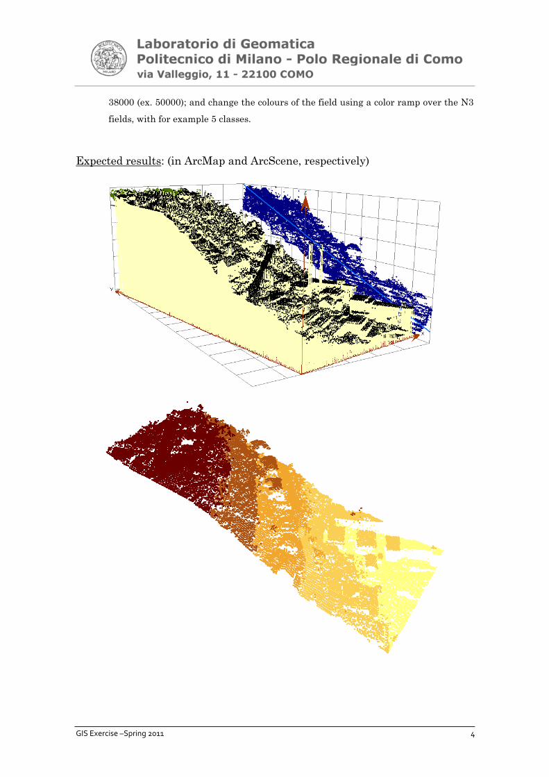
Classify -> Sampling – put a number higher than 38000 (ex. 50000); and change

the colours of the field using a color ramp over the N3 fields, with for example 5

classes.

GIS Exercise –Spring 2011 3

Expected result:

2. Visualization of the data in 3D

Two possible ways, ArcMap or ArcScene.

• ArcMap: enable the Geostatistical Analyst extension -> Customize -> Toolbars –

select Geostatistical Analyst; in the window Geostatistical Analyst -> Explore data ->

Trend Analysis; in the window you have to select as Layer=Lidar1Events and as

Attribute=N3.

• ArcScene: open the programme, Add data -> select the file Lidar1.dbf; right click on

the name Lidar 1 -> Display XY data – X field=N1, Y field=N2, Z field=N3; Properties

-> Quantities -> Quantity numbers: Classify -> Sampling – put a number higher than

GIS Exercise –Spring 2011 4

38000 (ex. 50000); and change the colours of the field using a color ramp over the N3

fields, with for example 5 classes.

Expected results: (in ArcMap and ArcScene, respectively)

GIS Exercise –Spring 2011 5

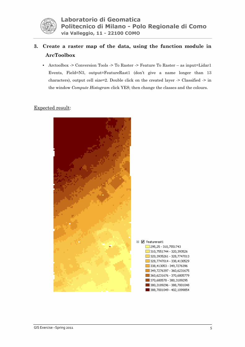
3. Create a raster map of the data, using the function module in

ArcToolbox

• Arctoolbox -> Conversion Tools -> To Raster -> Feature To Raster – as input=Lidar1

Events, Field=N3, output=FeatureRast1 (don’t give a name longer than 13

characters), output cell size=2. Double click on the created layer -> Classified -> in

the window Compute Histogram click YES; then change the classes and the colours.

Expected result:

GIS Exercise –Spring 2011 6

4. Use as interpolation method the inverse distance weighted with

different settings on the “lidar1” dataset:

The method is based on the assumption that the interpolating surface should

be influenced most by the nearby points and less by the more distant points.

• Arctoolbox -> 3D Analyst Tools -> Raster Interpolation -> IDW – Input Point

Features=Lidar1 Event, Z Field Values=N3, with these options:

MAP NAME interpolation1 interpolation2

POWER 2 2

SEARCH RADIUS TYPE variable fixed

N. OF POINTS 12

DISTANCE 20

OUTPUT CELL SIZE 2 2

Observe the results obtained, show differences between the two

output raster maps.

• Arctoolbox -> Spatial Analyst Tools -> Surface -> Cut Fill – Input before raster

surface=Interp1, Input after raster surface=Interp2, Output raster=IDW_CutFill.tif

• ArcToolbox -> Spatial Analyst Tools -> Map Algebra -> Raster Calculator; write

“Interp1” – “Interp2”

GIS Exercise –Spring 2011 7

Expected result:

Interpolation 1

Interpolation 2

GIS Exercise –Spring 2011 8

Reflect on the difference resulted from the different algorithms

employed in the interpolation process.

-----------------------------------------------------------------------------------------------------------

-----------------------------------------------------------------------------------------------------------

-----------------------------------------------------------------------------------------------------------

-----------------------------------------------------------------------------------------------------------

-----------------------------------------------------------------------------------------------------------

-----------------------------------------------------------------------------------------------------------

GIS Exercise –Spring 2011 9

-----------------------------------------------------------------------------------------------------------

-----------------------------------------------------------------------------------------------------------

5. Represent the data in Triangulated Irregular Networks (TIN)

ArcGIS supports the Delaunay triangulation method. To perform this

operation you have to use the 3D Analyst Tools:

• Arctoolbox -> 3D Analyst Tools -> TIN Management -> Create TIN – Output

TIN=TIN, Input Feature Class=Lidar1 Events, Height Field=N3

Expected result:

GIS Exercise –Spring 2011 10

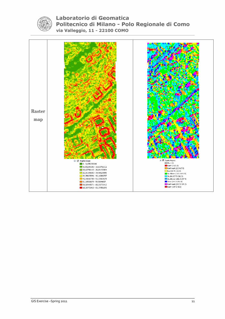
6. Calculate the slopes/aspects of the TIN and Raster maps

• For the TIN representation: right click on the layer TIN -> Properties -> Add -> face

slope with graduated color ramp, andf face aspect with graduated color ramp

• For the raster map: Arctoolbox -> 3D Analyst -> Raster surface -> slope -> Input

raster=raster, output measurement=DEGREE

Expected result:

Slope aspect

TIN

GIS Exercise –Spring 2011 11

Raster

map

GIS Exercise –Spring 2011 12

II. Data distribution

Data:

Lidar1.dbf

Task:

1. Compute the data distribution.

Are the data normally distributed?

Look at the histogram of the data distribution:

• Customize -> Toolbars -> Geostatistical Analyst -> Explore Data -> Histogram; Data

source=Lidar1 Events, Attribute=N3, Bars=10. Handling coincidental sample: choose

Include all

Expexted result:

GIS Exercise –Spring 2011 13

Statistic summary for the Lidar1 dataset:

Count 38008

Min 295,25

Max 404,08

Mean 356,17

1-st quartile 329,06

Median 356,85

3-nd quartile 385,86

Standard deviation 29,213

Skewness -0,15

Kurtosis 1,62

2. Statistical test

From the histogram we may note that the sample isn’t normally distributed.

As a matter of fact, we can apply a test of normality, taking into accounts

that in case of normality:

The null hypotheses are: H0: skewness = 0, kurtosis-3 = 0

We can calculate:

� Variate skewness =26αZ≤

N

skewness

� Variate kurtosis = 224

3αZ≤−

N

kurtosis

]6

,0[N

skewness N≈ ]24

,3[N

kurtosis N≈

GIS Exercise –Spring 2011 14

Probability Content from - ∞∞∞∞ to Z

With the help of the table, we get:

α=5: P=1-0.05/2=0.9750 � Za/2 = 1.96,

α=1: P=1-0.01/2=0.9950 � Za/2 = 2.575

GIS Exercise –Spring 2011 15

Results:

Value Test Result Test Result

Count 38008 Value α=5% α=1%

Skewness -0,15 Variate skewness 11,68 Not Normal Not Normal

Kurtosis 1.61 Variate kurtosis 55,13 Not Normal Not Normal

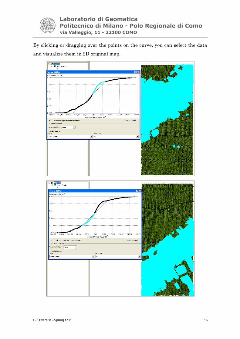
3. Data distribution calculation by Normal QQ Plot

Moreover we can verify the result by the normal QQ plot in ArcMap:

• Geostatistical Analyst -> Explore Data -> Normal QQ Plot; Data source=Lidar1

Events, Attribute=N3, Bars=10. Handling coincidental sample: choose Include all

As shown clearly in the normal QQ plot curve, the data in the set Lidar1.dbf

is not normally distributed. In fact if the data were normally distributed, the

curve would be similar to the line.

GIS Exercise –Spring 2011 16

By clicking or dragging over the points on the curve, you can select the data

and visualize them in 2D original map.

GIS Exercise –Spring 2011 17

III. One more case study on data distribution

Data:

piombino_eth.dbf

It is a digitized map of orthometric heights. The original map was at scale

1:25000.

Task:

Explore the data set piombino_eth.dbf.

1. Load the data piombino_eth.dbf

• Add data -> select the file piombino_eth.dbf

• Right click on the name piombino_eth.dbf -> Display XY data – put X

field=CAMPO1, Y field= CAMPO2, Z field= CAMPO3; change the reference

system clicking on Edit… -> … -> Monte Mario Italy1.prj

Change the visualization properties:

• Right click on the layer name -> Properties -> Quantities -> change the

colours of the field using a color ramp over the CAMPO3 field, with for

example 5 classes.

GIS Exercise –Spring 2011 18

Expexted results:

2. Compute the data distribution, showing the histogram and

calculating some statistics summary.

Are the data normally distributed?

Look at the histogram of the data distribution:

• Customize -> Toolbars -> Geostatistical Analyst -> Explore Data -> Histogram; Data

source=piombino_eth.dbf, Attribute=CAMPO3, Bars=10. Handling coincidental

sample: choose Include all

GIS Exercise –Spring 2011 19

Expexted result:

The statistic summary for the piombino_eth dataset are:

Count 5622

Min 0

Max 374

Mean 91,969

1-st quartile 25

Median 75

3-nd quartile 150

Standard deviation 69,712

Skewness 0,637

Kurtosis 2,854

Statistical test:

From the histogram we may note that the sample isn’t normally distributed.

As a matter of fact, if we apply a test of normality (the test will be conducted

exactly as the one in the previous section), we obtain:

GIS Exercise –Spring 2011 20

Value Test Result Test Result

Count 5622 Value α=5% α=1%

Skewness 0,638 Variate skewness 19,51 Not Normal Not Normal

Kurtosis 2,855 Variate kurtosis 2,23 Not Normal Normal

Moreover we can verify the result by the normal QQ plot in ArcMap:

• Geostatistical Analyst -> Explore Data -> Normal QQ Plot; Data

source=piombino_eth Events, Attribute=CAMPO3, Bars=10. Handling coincidental

sample: choose Include all

As shown clearly in the normal QQ plot curve, the data in the set

piombino_eth.dbf are not normally distributed.

Observation:

1. By comparing the QQ plot curve results of the data set Lidar.dbf and

piombino_eth.dbf, can you notice something particular? Try to explain the

abnormality.

GIS Exercise –Spring 2011 21

QQ plot curve of Lidar1.dbf:

QQ plot curve of piombino_eth.dbf:

3. Increase the numbers of bars contained in the histogram (as 100,

for instance)

Try to compare both histograms and try to draw some conclusions as well

from the observation. You obtain:

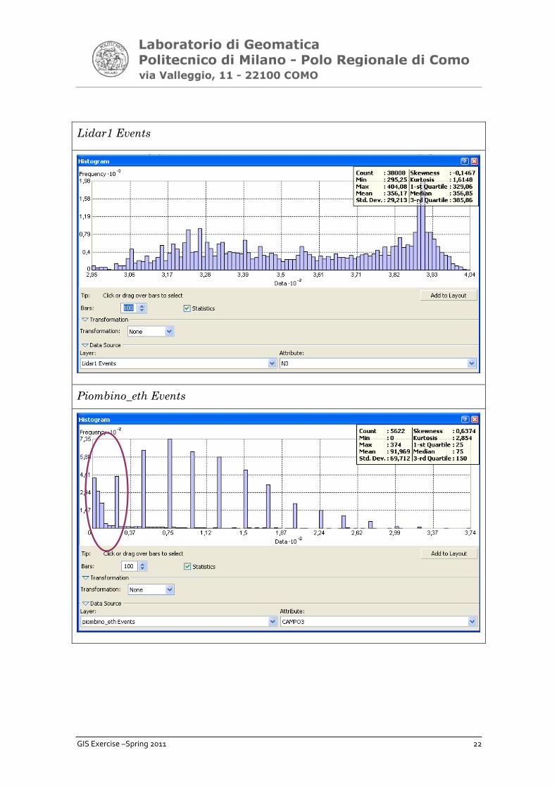
GIS Exercise –Spring 2011 22

Lidar1 Events

Piombino_eth Events