Electric Power Networks Efficiency and Security, Edited by Lamine Mili and James Momoh. ISBN 0-471-XXXXX-X Copyright © 2000 Wiley[Imprint], Inc.

Chapter 4.2

GIS-Based Simulation Studies for Power Systems Education

Ralph D. Badinelli1, Virgilio Centeno2, Boonyarit Intiyot3

1. Professor, Department of Business Information Technology, Pamplin College of Business, Virginia Tech

2. Associate Professor, Bradley Department of Electrical Engineering, Virginia Tech 3. Graduate Research Assistant, Department of Industrial and Systems Engineering,

Virginia Tech

Editor’s Summary: This chapter advocates the application of two educational methods,

namely case studies and decision modeling, as the best way to teach design and

management methods in power systems. A sample of case studies is presented, which

includes public policy studies aimed at transmission and generation expansion subject to

a cap on electricity prices and generation emissions. The second educational approach

makes use of the structured decision modeling under multiple, conflicting performance

measures; the objective is to seek a set of desirable and feasible solutions among

numerous alternatives. As illustrative examples, the authors discuss several interesting

case studies that deal with the selection of the right site and size of DG or of FACTS to

mitigate instabilities in power systems. Furthermore, examples of simulation results are

presented to illustrate the cost, spatial, and temporal relationship of the interconnection of

the DG to the distribution feeders. A very comprehensive formulation of unit

commitment is examined too. The chapter also includes the description of the working

software package that the authors developed. Termed the Virginia Tech Electricity Grid

and Market Simulator (VTEGMS), the main component of this package makes use of

2

object-oriented programming as a means to maximize the robustness and flexibility of the

software. A good reference of available optimization methods and simulation packages

are summarized in the quoted references and in a table of comparison of software.

$.1 Overview In this chapter we prescribe computer simulation as a robust tool that should be

integrated into any comprehensive educational curriculum in the field of power systems

design, engineering and management. Our advocacy of computer simulation is based on

the essential role that this methodology plays in two foundational elements of power

systems education – case studies and decision modeling. These elements, in turn, are

necessary in the education of future power-system designers, engineers and managers

who need to understand the ever-expanding complexities of these systems from the points

of view of their many stakeholders. Computer simulation is unique among modeling

techniques to support case analysis and decision modeling for such complex systems. In

conjunction with case studies, text and lecture materials computer simulation forms a

flexible educational support system (ESS). In this chapter we will provide an overview

of the role of case analysis and decision modeling in power-systems education and the

basic elements of simulation models along with an explanation of the essential role they

play in this education.

We are motivated by two concomitant features of the educational landscape.

First, the important role played by power systems in the economic health, environmental

quality and national security of the United States and other countries has become evident.

As a consequence, operation, design and management of power systems have become

disciplines that are gaining in popularity and importance. Second, the operation, design

and management of power systems involve large numbers of inter-related systems that

are mutually dependent in mathematically complex ways. New developments in

generation technologies, market deregulation, environmental regulations, reliability

standards and security concerns are aggravating the complexity and interdisciplinary

nature of this topic. New and existing personnel in the fields of power-system

engineering, grid operation, power plant control, energy portfolio management, public-

3

policy and consulting demand up-to-date and holistic education in the rapidly changing

power-systems discipline.

Decision making is the common foundation of all of the challenges in the fields

mentioned above and we view all learners as future decision makers. Hence, our design

of educational tools will revolve around decision analysis. Examples of the decision

domains that our educational tool must support include,

• Public policy decision problems - environmental policy planning, market

regulation planning, infrastructure planning

• Engineering decision problems – protection system design, generation and

transmission technology selection

• Business decision problems –generation capacity planning, unit commitment,

optimal dispatch, demand side response, trading strategy, financial risk

management

For each of these decision problems the cause-effect relationship between

decision alternatives and key performance indicators (KPI) such as cost, reliability,

pollution, market equity, etc. must be understood and analyzed by the decision maker.

For the learner, modeling the decision of a case study is the most effective method for

identifying the tradeoffs inherent in the KPIs. The learning process can be brought to

fruition only by quantifying these tradeoffs and experimenting with the cause-effect

relationship inherent in each decision – a task that demands computer simulation.

Electric generation units, power grids and energy markets form a complex system

that evolves over time through the decisions of system managers, engineers, unit

operators and market participants as well as through the influence of weather, load

variation, market prices, forced outages and the physical behavior of network

components. Some of these influences have a random component to their variations over

time making the trajectory of the power system stochastic. Computer simulation is

unique among modeling techniques in its ability to capture the effects of numerous

interacting influences as well as of randomness on the performance of a system.

Furthermore, the raw output of a simulation in the form of the trajectory of performance

measures over time can be summarized in statistically valid ways to evaluate the long-run

behavior of a system over time and over a representative sample of random scenarios.

4

$.1.1 Case studies

A case study is a presentation of a problem in the context of realistic conditions,

people and events. Unlike traditional textbook problems, a case study does not present a

well-formulated problem but rather a situation of conflicting needs and desires instigated

by the disparate points of view of various stakeholders. Each case presents the learner

with a situation in which a decision is needed. The learning process is pursued through

the learner’s attempts to create a model of the decision problem and to use the model to

determine the best choice of alternatives. See Bodily, 2004 [7].

Case studies are the most effective form of learning assignment for the education

of professionals for several reasons (see Barnes, Christensen, and Hansen, 1994 and

Wasserman, 1994):

• Students become active instead of passive learners. Students learn by doing.

• Students are forced to define questions, not just answers.

• Students must identify, respect and consider several points of view on a

problem.

• Students are forced to apply theory in order to create structure for the case as

opposed to applying a structured method to a well-defined, contrived problem.

• Students are forced to compromise and look for workable, feasible solutions

when there are conflicting needs and constraints.

• Students acquire general problem-solving skills within a field of study instead

of mere formulaic solution methods that, in real situations, must be applied

with modifications and adjustments in consideration of assumptions that are

not met and factors that were ignored in the development of the methods.

• Students gain maturity and confidence by facing the ambiguity of realistic

cases.

In every industry the decision problems that comprise the public policy,

engineering and management naturally fall into a hierarchical order. The solutions to

decision problems that have long-term consequences and that are updated infrequently

become parameters that influence decisions that have shorter-term consequences and that

can be updated more frequently. For example, the choice of technology for a new

5

generation unit will influence the way that this unit is committed and dispatched. Hence,

a hierarchy of decisions emerges in which longer-range, less-frequent decisions are

placed above shorter-range, more frequent decisions. We assert that a holistic

understanding of a subject such as the design, engineering and management of power

systems requires the learner to attempt to solve all of the essential decision problems

associated within this subject as well as to see these decision problems in their

hierarchical order. A collection of case studies in hierarchical order integrated with text

and lecture material comprises a well-designed educational experience for future

professionals in the field of powers systems.

The list below forms such a collection. These cases include problems of

operating a conventional power system as well as problems of designing and operating

power systems of the future.

Level 1: Public Policy Cases

• How to set the emissions limits on generation units in a given power grid

• How to limit the prices that can be cleared in a given power market

• How to limit the prices that can be charged to different consumer groups in a

given power market

• Where to install new transmission lines, gas pipelines or publicly-owned

generation in a given power grid

Level 2: Power Systems Design Cases

• How to select non-traditional generation technologies for distributed generation

(DG)

• How to select the best location for DG.

• How to select the type of generation plant to add to a given power grid

• How to plan the installation of new capacity in a given power grid

• How to coordinate protective devices for a given power grid.

• How and where to change protection coordination for DG.

• How to select fast, alternating-current transmission (FACT) devices to strengthen

transmission systems.

6

• How to coordinate protections and placement of FACT devices for voluntary

islanding during catastrophic events.

• How to determine locations that are exposed to catastrophic hidden failures.

Level 3: Power Systems Management Cases

• How to set circuit breaker limits in a given power grid

• How to configure FACT controllers. See Acha, et. al., 2004.

• How to commit the generation units to a given power grid

• How to dispatch the generation units in a given power grid

• How to bid or offer energy in a wholesale energy market for a given power grid

• How to configure a portfolio of financial derivatives to support the risk

management of an energy trading position within a given power market

• How to commit and dispatch generation units to a power grid that is practicing

various forms of

o DSR

o environmental restrictions

o market regulations

o demand growth rates

o fuel cost volatility

• How to encourage consumers to shape load in order to balance cost and

convenience.

The educational cases have several unique characteristics that carry the learner

through these decisions in a realistic manner:

• Interactive – students are able to change different aspects of a power system’s

elements, markets or regulatory environment in order to experiment with different

scenarios for the configurations of physical assets, time series of loads and

failures, location and type of generation, contractual arrangements between

customers and suppliers and regulatory constraints. For each scenario entered by

a student, the KPIs of the system must be computed by a computerized model.

7

• Realistic – the educational cases are based on prototypes of real and proposed

power systems, markets and regulatory environments.

• Configurable – the development of a case-based ESS will yield not only a sample

of case studies for use in courses, but also structures for the database, student

interface and cases that can be modified with new data for the development of

new case studies.

Clearly, a qualitative overview of the decision problems listed above does not

prepare a prospective power systems engineer, manager or regulator for the real world.

An understanding of the tradeoffs presented by these decision problems requires a

quantitative analysis of them. Decision support systems that are more sophisticated than

a collection of simple formulas are necessary. Specifically, our case analyses require

decision support systems that embody mathematical decision models.

Many powerful methodologies for building and optimizing decision models have

been developed over the last fifty years. The lexicon of modeling tools includes

computer simulation, linear programming, integer programming, nonlinear programming,

dynamic programming and many others. Momoh (2004) provides a comprehensive

overview of decision models for power-system cases and their associated optimization

methods. Although these methodologies have been available for several decades, they

have not enjoyed rapid adoption by businesses and institutions. One reason for their slow

adoption is that most people find model formulation very difficult. The computerized

tools for describing and prescribing solutions can be applied only after a descriptive

decision model has been created -- a task that generally is accomplished through the art

and science of an operations researcher who understands the problem domain and the

structure of decision models. For the practicing manager or analyst, model application is

the process that delivers business performance. Therefore, our educational goal is to

teach the application of models to the decision problems described earlier.

A general understanding of the structure of decision models and their application

is necessary for both the learner and the teacher. We provide such an overview below.

8

$.1.2 Generic decision model structure

A decision model quantifies the cause-effect relationships between actions and

outcomes. The outcomes of an action are expressed in terms of performance measures,

which, for any decision alternative, are used by the decision maker to determine the

alternative’s feasibility and desirability. For example, the performance measures for the

unit dispatch decision in a given time period include the total cost of generation across all

dispatched units, the total grid power loss, the line load on each transmission line, the

load coverage for each load bus, the reliability of the system, etc. To the challenge of

quantifying these performance measures we propose the application of decision models.

Models are the brains within a decision support system that transform masses of data into

knowledge.

In order to specify the scope of the decision the modeler categorizes the causative

factors into two sets: a set of controllable factors that are used to define the alternatives

available to the decision maker and a set of uncontrollable influences on the performance

measures.

The alternatives of a decision represent the choices, options or actions that a

decision maker is empowered to execute within the scope of a given decision.

Mathematically, we must represent these alternatives in terms of a well-defined set of

data elements that we call decision variables. For example, the alternatives for the unit

dispatch decision in a given time period can be represented by the set of power output

values for each generation unit that is available. This vector of power output values

would constitute the decision variables for this decision. Among all of the possible sets

of values for the decision variables, the decision maker seeks the one that yields the most

desirable, feasible performance. This solution is called the optimal solution to the

decision problem for which the model is built.

The uncontrollable factors of a decision are the influences on the performance

measures that cannot be chosen by the decision maker. We call these uncontrollable

factors parameters. For example, the parameters of the unit dispatch decision for a given

time period include the capacities of each available generation unit, the thermal capacity

of each transmission line, the real and reactive load at each load bus, the coefficients of

the operating cost function of each available generation unit, etc. A parameter could

9

remain constant throughout the analysis or could be a random variable. If some

parameters are random variables, then the performance measures that depend on these

parameters also are random variables – a characteristic of the model that earns it the label

“stochastic”. Parameters, or their probability distributions, must be measured, estimated

or forecasted in order to build the database for a decision model.

Contrary to common belief, the presence of random parameters does not preclude

the application of decision models. In fact, the ability to model decision-making under

conditions of uncertainty can be considered the highest form of the modeler’s science. In

order to construct a stochastic model we must make use of the probability distributions of

the random parameters. Doing so requires specification of these probability distributions

as, for example, the estimates of the mean and the standard deviation define the

probability distribution of a normally distributed parameter and the coefficients and

volatility of a mean-reversion forecasting formula define the probability distribution of a

future commodity price.

Performance measures that cannot be predicted with certainty introduce the

element of risk into the decision. In these cases, the distributions of random performance

measures must be summarized over all scenarios into measures that capture both risk and

reward. For example, for the unit dispatch decision in a given time period the total cost

of generation is a random variable because the total load is not known with certainty in

advance. Variations in the load from its forecasted value are handled by automatic

dispatch of reserve power. Consequently, the actual total cost of power generated during

the given time period can be predicted by a decision model only up to the probability

distribution of this cost. Summarizing this probability distribution over all possible load

scenarios in terms several summary measures such as the distribution’s mean and its

upper and lower quartile points gives the decision maker a representation of expected

financial cost as well as the risk associated with this cost.

Most decision alternatives associated with the design and management of a power

system have ramifications that extend over long time horizons. The trajectory of a

performance measure over a time horizon can exhibit various kinds of cyclic, trended or

memory-influenced behavior. In order to provide useful indicators of the performance of

an alternative, a decision model must summarize these trajectories over a time horizon

10

that is long enough to capture all of the time-varying behavior of the performance

measures. For example, for the unit dispatch decision over multiple time periods the total

cost of generation will exhibit fluctuations and memory due to load variation over time,

load momentum, generator startup costs and ramping constraints. Summarizing the time

series of generation cost in terms of its time average provides the decision maker with a

useful indicator of overall cost performance. When a model summarizes performance

measures over random scenarios and over time, as necessary, the resulting measures are

called key performance indicators (KPI) as they are used directly to evaluate the

feasibility and desirability of each alternative.

In order to specify the feasibility and desirability of performance, the decision

maker imposes a decision criterion on each KPI. There are two possible forms for each

criterion: a KPI can be constrained from above or below in order to impose bounds on

performance or a KPI can be maximized or minimized in order to pursue performance to

its greatest possible extent.

The cause-effect relationships from decision variables and parameters to KPI’s

form a descriptive decision model. The qualifier “descriptive” indicates that the model’s

value is to predict or describe the performance of a system for a hypothetical set of inputs

to that system. Hence, a computerized descriptive model provides the decision maker

with an efficient means to test any proposed alternative and a trial-and-error capability

for searching for the best alternative. Given enough time, the decision maker can arrive

at an alternative that yields optimal or near-optimal, feasible performance.

Some decision models can also help select the best course of action from among

an overwhelmingly large set of alternatives. An extension of a descriptive model engages

a computerized search algorithm that, in effect, automatically performs an, intelligent

trial-and-error procedure for the decision maker. Such an extended model is called a

prescriptive model. Prescriptive models provide dramatically enhanced decision support

when a decision involves so many feasible alternatives that manual trial-and-error is

impractical.

The first step in building a decision model is to define data elements and to derive

the mathematical relationships that constitute the descriptive model. The categories of

data elements are:

11

• Decision variables

• Parameters

• Performance measures

• KPI’s

• Criteria

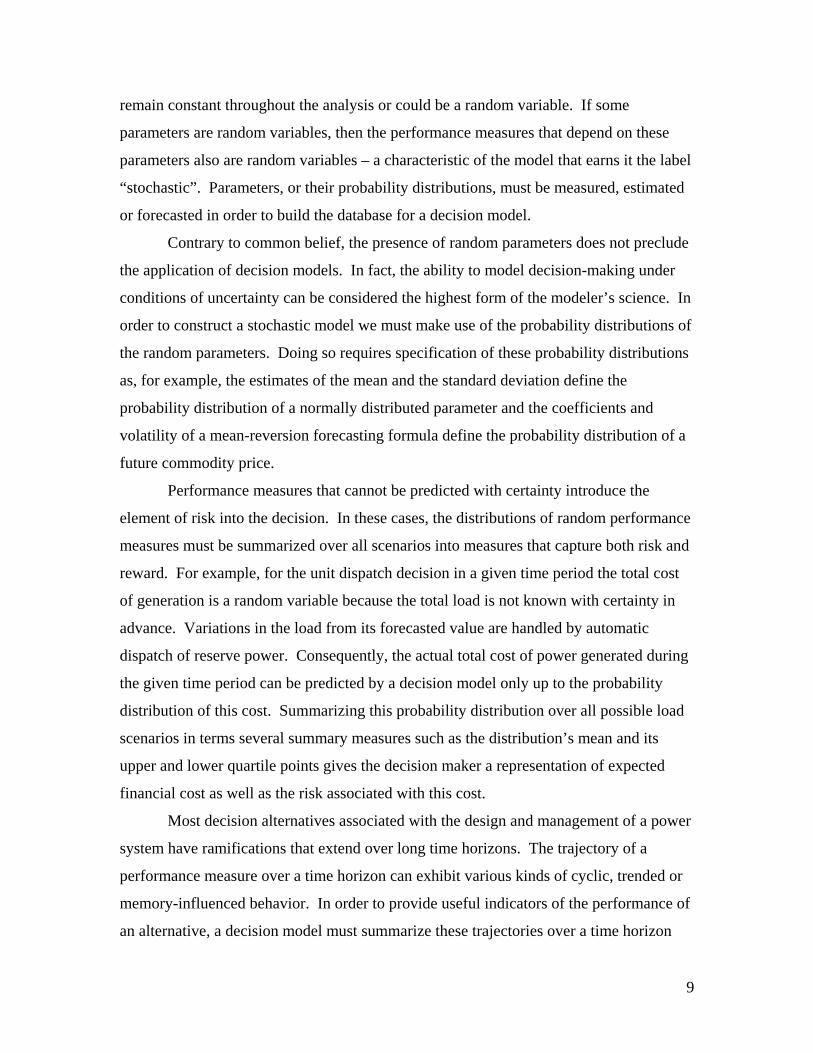
$-1 shows the general structure of a decision model. The most important perspective to

draw from Figure $-1 is the fact that a descriptive model forms the core of a prescriptive

model. Furthermore, the search routine of the prescriptive model is usually performed by

a commercially available code of a search algorithm (e.g., linear programming, integer

programming, etc.). However, the rest of the construction in Figure $-1, without which

the search routine is useless, is the responsibility of the modeler.

12

DV Decision Variables

Cause-effect relationships from decision variables and parameters to performance

measures

Descriptive Functions

PM Performance measures

PARMS Model Parameter Database

Performance measures that

are random variables or time-varying

are summarized into one or a

few measures

Scenario & Time

Summary

KPIKey

performance indicators

DBMSPower System

Database

Each KPI is placed in a constraint or

the objective function

Decision CriteriaAn optimal solution

is found by intelligent trial-and-error evalution of

the criteria for different choices of

the DV's

Search Routine

OPT Optimal Solution

CRIT Criteria evaluation – feasibility and desirability

Descriptive Model

Prescriptive Model

Figure $-1: The data flow of descriptive and prescriptive models

$.1.3 Simulation modeling

Decisions related to power systems have outcomes (performance measures) that

play out over a long time and that can take on many scenarios due to randomness in

system parameters such as loads and market prices. Furthermore, the relationship

between decision variables and performance measures for power-systems decision

problems is typically very complex and nonlinear. Of all of the forms of decision

modeling, simulation is uniquely capable of capturing complex cause-effect relationships,

time varying performance measures and stochastic effects. In fact, for many of the

13

decision problems that the learner needs to model, simulation is the only modeling

technique that can produce a reasonably accurate descriptive model. For example,

simulation can be used to identify the vulnerabilities of the protection system prompted

by the interconnection of DG to a distribution feeder. By comparing the total DG short-

circuit contribution passing through protection devices with the pick up settings of the

devices the required protection coordination changes for a specific DG location can be

determined, Depablos (2004). Figure $-2 shows a simulation of a fault at bus 2 that

results in a DG short-circuit contribution greater than the pick up setting of the protective

device B. This will clearly result in miss-operation of unit B and unnecessary loss of

load.

Figure $-2: Effect of DG insertion in the coordination of protective devices.

Every simulation model is a computerized description of a system. A system can

often be visualized as a collection of interacting operations with flows of material, power,

cash or other commodities among them. The simulation model tracks the state of the

system as it evolves over time through the occurrence of events such as changes in load,

outages, unit dispatching, short circuits and the passage of time. In order to do this a

simulation model is created in the form of a computer program that consists of the

following fundamental elements.

• Random Number Generator

• Event Scheduler

14

• State Transition Procedures

• System State Data Management

• Performance Measure Output

Through the creation of an artificial clock that marks simulated system time

the simulation program schedules the events that cause the system to evolve.

Transitions in the state of the system take place at points in time determined by the

Event Scheduler. In the case of a typical simulation of a power grid, the Event

Scheduler would be programmed to update the time on an hourly basis. At each of

these transition times, the State Transition Procedures update the state of the

simulated power system to reflect changes caused by the events that occur at the

transition time. The current state of the system is represented by the System State

Data. The System State Data is used by the Performance Measure Output routines to

store values of performance measures over the time period that has just ended. Once

the updated performance measures are filed, the simulation program returns to the

Event Scheduler to process the next system-changing event.

Some of the state-changing events, such as load variations and outages may be

the result of random effects. Computer simulation models are able to introduce

random events into the event schedule through the use of random number generators.

Through this mechanism, computer simulation models can represent realistically the

performance that results from planned system interventions as well as unplanned

system influences.

Events are defined by the modeler in terms of the simplest changes that can

take place in the system that is modeled. By modeling the detailed interactions of

system components over small intervals of time and aggregating the results of these

interactions complex behavior can be described through the use of numerous,

relatively simple transition procedures. In fact, computer simulation is the only

modeling technique that can capture the complexity and randomness of a typical

power system.

In a simulation model of a power system, the power flows through each

network element and the cash flows associated with the power flows can be modeled

for each hour of each day. From hour to hour, the simulation program updates the

15

status of each generation unit, load and network element and stores this status in

computer memory. The performance measures of the power system are computed

and the results filed.

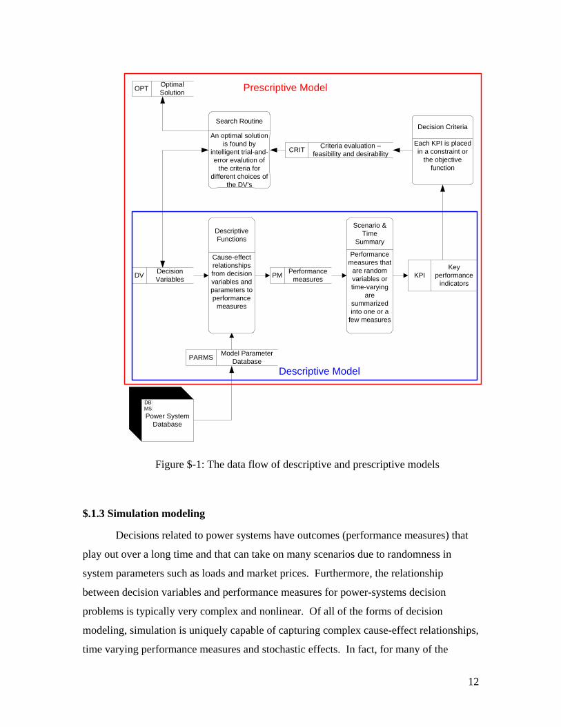
Another simple example of simulation modeling is found in the case of the

unit dispatch decision. The simulation model for this decision would compute, for

any given dispatching plan and for any given scenario of loads, the total generation

cost as well as other performance measures. $-3 portrays a time series of generation

costs over a 24-hour period for one scenario of loads. This time series would be

summarized most appropriately in terms of its average. A simulation model could

generate this time series if the scenario of loads was provided as input parameters.

We call the computation of performance measures over a time horizon for one

scenario of parameters a “replication” of the simulation model.

Generation Cost Time Series

0

1000

2000

3000

4000

5000

6000

7000

1 2 3 4 5 6 7 8 9 10 11 12 13 14 15 16 17 18 19 20 21 22 23 24Hour

$ th

ousa

nds

Figure $-3: Generation cost time series example

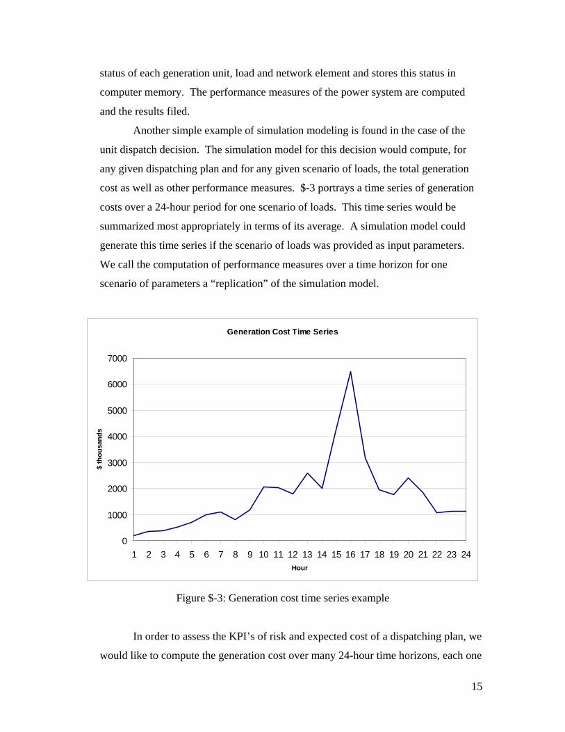
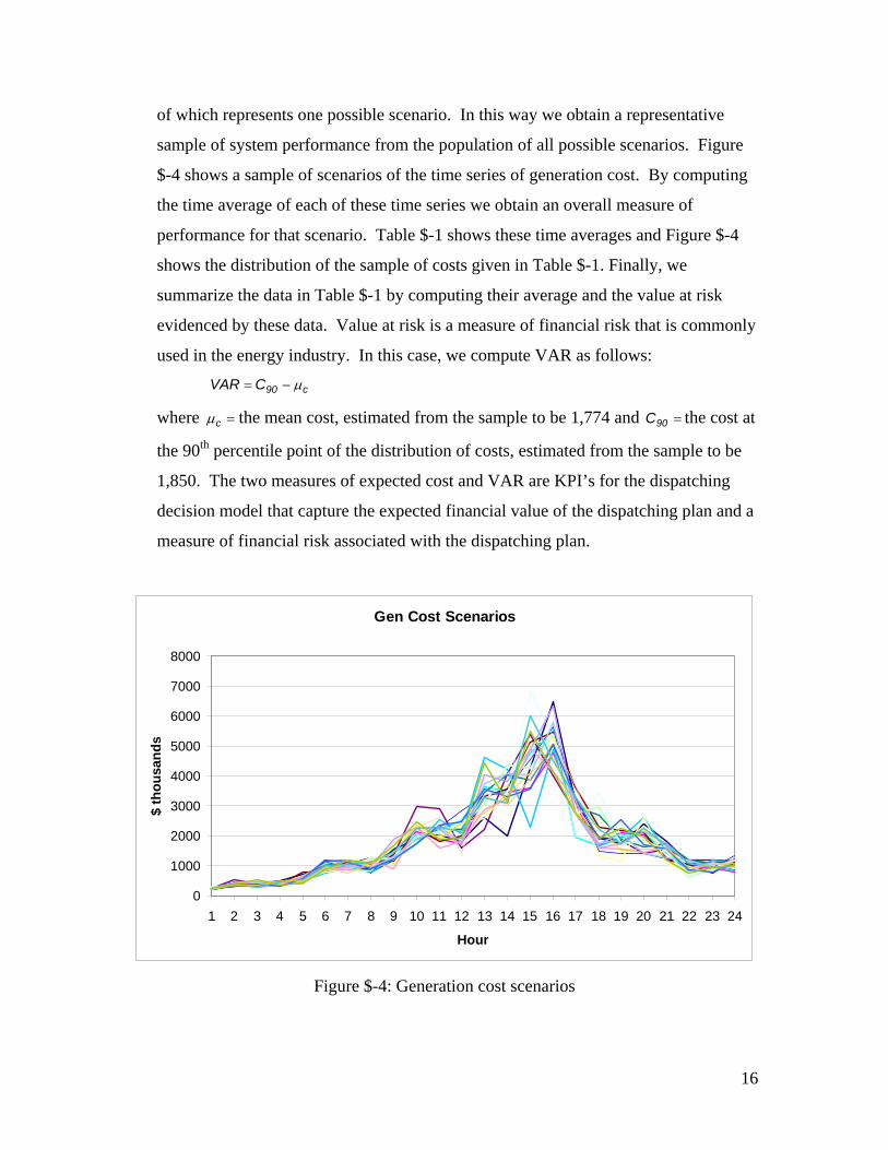
In order to assess the KPI’s of risk and expected cost of a dispatching plan, we

would like to compute the generation cost over many 24-hour time horizons, each one

16

of which represents one possible scenario. In this way we obtain a representative

sample of system performance from the population of all possible scenarios. Figure

$-4 shows a sample of scenarios of the time series of generation cost. By computing

the time average of each of these time series we obtain an overall measure of

performance for that scenario. Table $-1 shows these time averages and Figure $-4

shows the distribution of the sample of costs given in Table $-1. Finally, we

summarize the data in Table $-1 by computing their average and the value at risk

evidenced by these data. Value at risk is a measure of financial risk that is commonly

used in the energy industry. In this case, we compute VAR as follows:

c90CVAR μ−=

where =cμ the mean cost, estimated from the sample to be 1,774 and =90C the cost at

the 90th percentile point of the distribution of costs, estimated from the sample to be

1,850. The two measures of expected cost and VAR are KPI’s for the dispatching

decision model that capture the expected financial value of the dispatching plan and a

measure of financial risk associated with the dispatching plan.

Gen Cost Scenarios

0

1000

2000

3000

4000

5000

6000

7000

8000

1 2 3 4 5 6 7 8 9 10 11 12 13 14 15 16 17 18 19 20 21 22 23 24

Hour

$ th

ousa

nds

Figure $-4: Generation cost scenarios

17

Table $-1: Scenario Averages

Scenario Average Cost 1 1742 2 1683 3 1807 4 1778 5 1782 6 1847 7 1791 8 1790 9 1734 10 1875 11 1799 12 1724 13 1757 14 1632 15 1875 16 1794 17 1753 18 1841 19 1793 20 1692

Average= 1774 VAR= 76

Distribution of Cost

0

1

2

3

4

5

6

7

8

9

< 1,691 1,691 - 1,744 1,744 - 1,797 1,797 - 1,850 > 1,875

Figure $-5: Distribution of Sample of Costs

18

$.1.4 Interfacing

As a practical matter, a computerized educational support system is effective only

if its interfaces for learners and teachers are transparent and easy to learn. To these users

of a simulation program, the simulation is a tool for analyzing tradeoffs associated with

decisions related to the design and management of a power system. Clearly, the

underlying details of the simulation model, such as random number generators, statistical

evaluation of performance measures, event scheduling should be hidden from these users.

The learner’s interface to the simulation package should be designed for entry of decision

variables and viewing of KPI’s that result from these settings of the decision variables.

The teacher’s interface should include the ability to modify the parameter database in

order to create different configurations of a power system for different sets of learners.

One of the most natural representations of the assets of a power system is that of a

geographic information system (GIS). A GIS is fundamentally a database of objects,

each of which can be indexed by a location in terms of an x-coordinate, a y-coordinate

and elevation coupled with a graphical interface that displays these objects on a map.

Generation units, power lines, transformers, substations, and buildings or other sites

where loads occur can be represented in a GIS database and displayed on a computer

screen so that a learner or a teacher can see clearly the components that make up the

power system under study. In addition, GIS provides a connection that permits linking

the physical and economic databases of the electric grid to available sociopolitical

databases, opening the possibility to study the effect public policy, public perception and

other sociopolitical factors that influence decision makers in real systems. Coupling the

GIS system to the simulation program provides a seamless interface for the user between

data entry and KPI’s. Figure $-6 shows a flow chart of the kind of ESS that we advocate

in this paper.

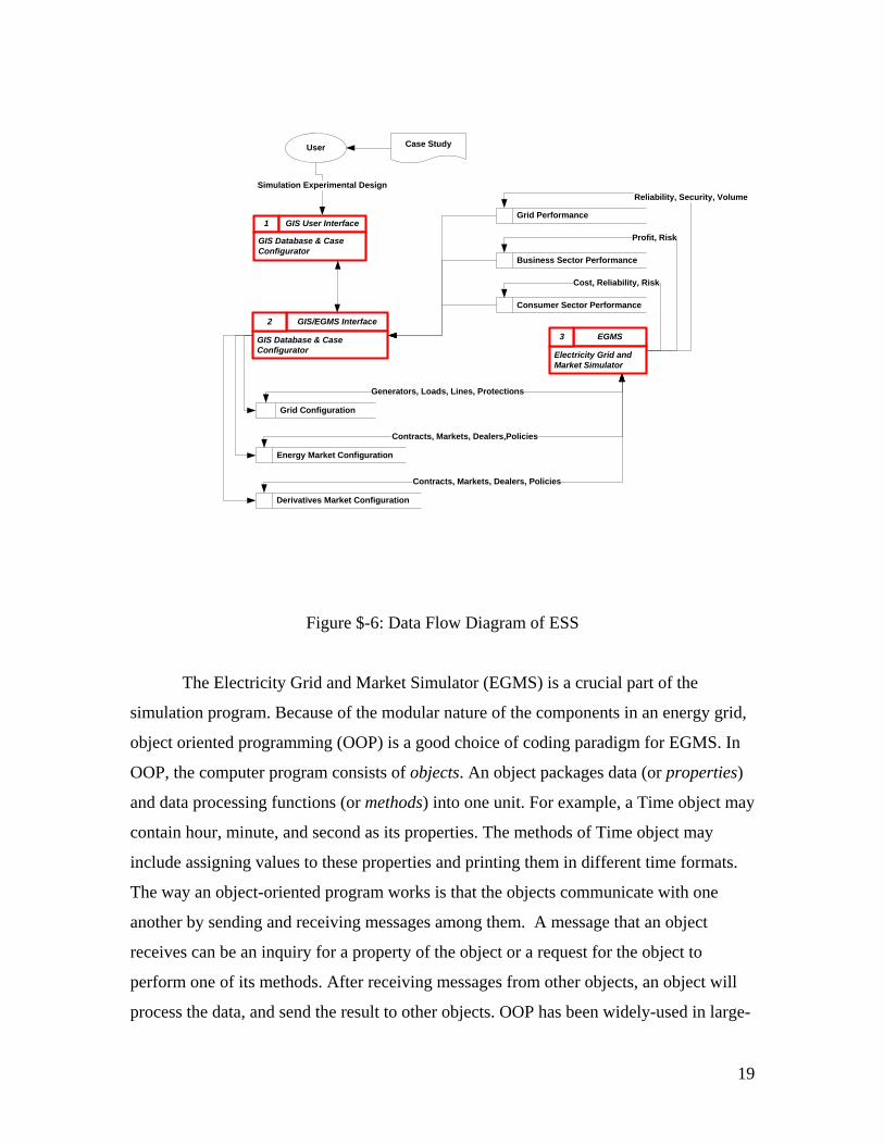
19

Grid Performance

Business Sector Performance

Consumer Sector Performance

Reliability, Security, Volume

Profit, Risk

Cost, Reliability, Risk

User

Simulation Experimental Design

Grid Configuration

Energy Market Configuration

Derivatives Market Configuration

Generators, Loads, Lines, Protections

Contracts, Markets, Dealers,Policies

Contracts, Markets, Dealers, Policies

1 GIS User Interface

GIS Database & Case Configurator

Case Study

EGMS

Electricity Grid and Market Simulator

3

GIS/EGMS Interface

GIS Database & Case Configurator

2

Figure $-6: Data Flow Diagram of ESS

The Electricity Grid and Market Simulator (EGMS) is a crucial part of the

simulation program. Because of the modular nature of the components in an energy grid,

object oriented programming (OOP) is a good choice of coding paradigm for EGMS. In

OOP, the computer program consists of objects. An object packages data (or properties)

and data processing functions (or methods) into one unit. For example, a Time object may

contain hour, minute, and second as its properties. The methods of Time object may

include assigning values to these properties and printing them in different time formats.

The way an object-oriented program works is that the objects communicate with one

another by sending and receiving messages among them. A message that an object

receives can be an inquiry for a property of the object or a request for the object to

perform one of its methods. After receiving messages from other objects, an object will

process the data, and send the result to other objects. OOP has been widely-used in large-

20

scale software development for years because of the modularity, expandability, and

reusability of the code. Unlike the traditional programming, keeping the OOP code up-to-

date is relatively easy and cost-effective. These advantages are so compelling that we

cannot imagine coding an EGMS without OOP.

In order to program EGMS using OOP, we define the following main objects:

1. Grid Operations Model (GOM) is an object that simulates planning,

scheduling, dispatching and controlling an electrical grid.

2. Risk Management Model (RMM) is an object that assesses the financial risk

and develops strategies to manage it.

3. Energy Market Model (EMM) is an object that evaluates market

performance.

4. System Configuration Model (SCM), Simulation Controller (SC), Output

Stream Summarizer (OSS), Output Statistical Analyzer (OSA) are objects

for the management of the simulation program, data entry and output

reporting.

Figure $-7 depicts the relationships among these objects. When the simulator

runs, GOM reads the grid configuration, simulates the electricity flows, and updates the

grid performance. RMM reads the grid performance and derivatives market

configuration, performs risk analysis, and updates the risk portfolio performance. EMM

reads the risk portfolio performance as well as the market configuration and grid

performance and outputs the consumer sector performance and business-sector

performance. All of these events are executed for each time interval of the simulation.

21

3.1 SCM

System Configuration ModelUpdates the database that defines electrical grid and energy markets

3.2 EMM

Energy Market Model

3.3 RMM

Risk Management Model

3.4 GOM

Grid Operations Model

DFD level 2

Grid Configuration

Energy Market Configuration

Derivatives Market Configuration

Simulation Experiment Design

Horizon, Reps, Factors

Generators, Loads, Lines, Protections

Contracts, Markets, Dealers, Policies

Contracts, Markets, Dealers, Policies

User

3.5 SC

Simulation ControllerGenerates Random NumbersSchedules IterationsRecords Output Scenarios

Grid Performance

Business Performance

Consumer Performance

Reliability, Security, Volume, Spot Prices

Profit, Risk

Cost, Reliability, Risk

Cash Flows

Risk Portfolio Performance

Price Variations

Load Variations

Price Variations

3.7 OSA

Output Statistical Analyzer

Load VariationsLoad Variations

3.6 OSS

Output Stream SummarizerSummarizes the output streams from each replication

Replication Summary

Response Surface

Figure $-7: Data flow diagram of EGMS

To simulate the power flows with GOM, we need to solve a set of power-flow

optimization problems (see Momoh 2001). Solving such optimization problems is the

22

most computationally intensive part of the simulator. Since the flows must be updated for

every simulated time interval, the speed of the simulator could become a problem if the

code for solving the optimization problems is not efficient. Writing an efficient

optimization routine from scratch could be very time-consuming. Fortunately, some

proprietary software packages, such as CPLEX and IMSL, provide routines for these

purposes. With years of research and development invested in these software packages,

their routines are proven to be efficient and reliable. Consequently, the construction of

EGMS should be integrated with these routines.

23

$.2 Concepts for modeling power system management and control

The determination of optimal power flow in a grid over a sequence of time

periods can be modeled as a set of decisions and actions that execute the workings of the

energy markets and the technical control of the electricity grid. In the operation of real

energy markets and grids as well as in a simulation of these systems, the operational

decisions are supported by computerized models. These models manifest several

challenging features of mathematical modeling and optimization, which we describe

below in a constructive sequence.

$.2.1 Large-scale optimization and hierarchical planning

The control of markets and electricity grids requires coordinated decision-making

across five decision domains.

1. Configuring: installed generation capacity, grid configuration, market regulations

2. Planning: bi-lateral contracts, wholesale bids & offers, unit availability

3. Scheduling: unit commitment, ancillary service contracts, reserve requirements

4. Dispatching: unit dispatch, demand management, regulation

5. Controlling: voltage control, frequency control, circuit protection

The large number of variables that these decisions encompass classifies this

collection of decisions as a large-scale optimization problem. There is no practical

decision-support system that can simultaneously optimize all of these decisions.

Consequently, power grid and market management is carried out through the application

of some conventional heuristic approaches.

A heuristic approach that is often used is one that is based on a hierarchical

sequence of decisions that lead, through successive levels of detail, to a final solution.

The basic idea behind hierarchical planning is that the solution to a rough-cut

representation of a decision in terms of aggregated decision variables can serve as a set of

guidelines and constraints for a refined decision in terms of detailed decision variables.

In other words, the final solution to a problem can be achieved by first “coarse-tuning”

the solution and then “fine-tuning” the solution.

In the case of energy grid management, the conventional hierarchy of decision

making conforms to the ordered list shown earlier. For example, the problems of

24

determining the unit availability, unit commitment and unit dispatch are all related

through performance measures such as profit and service level, which depend on all of

these three decisions. Rather than attempt to find solutions to all three decisions

simultaneously so that a globally optimal solution is obtained, a hierarchical planning

approach would specify three separate decisions to be solved in stages. The

determination of unit availability, based on approximate representations of total demand

over the upcoming week, provides capacity constraints on the commitment and

dispatching decisions. The commitment decision, based on a forecast of load variations

over the next 36 hours for which real-time dispatching will be needed, consumes the bulk

of the generation capacity and leaves a judicious amount of capacity for support of the

imbalance dispatching decisions.

The intuitive appeal of this approach is found in the selection of decision

variables for each level of the hierarchical planning process. The first level generally,

involves strategic decisions that have long-term effects such as unit availability. The

second level involves decision variables that describe how the available assets are to be

committed. The third level involves decision variables that describe how committed

assets are to be dispatched. The fourth level and fifth levels involve decision variables

that describe how dispatched assets are to be controlled. Under the hierarchical scheme,

long-range, strategic decisions are made first. These decisions then impose constraints on

the shorter-range, more detailed decisions that follow. At each level the plan for the

entire system is developed in more detail.

The approximation inherent in hierarchical planning is introduced in the modeling

of the performance of lower-level solutions at any stage in the hierarchy. In order to

simplify each stage’s problem, the effects of the lower-level decision variables on the

current stage’s constraints and the objective function are approximated. In turn, the

solution to a higher-level problem specifies constraints on the next lower-level problem,

and so on.

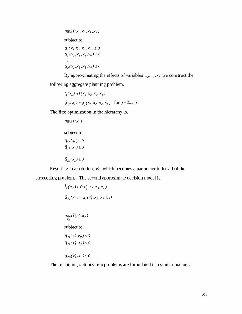
Using the “hat” notation to indicate approximations, the hierarchical planning

approach is described as follows:

Suppose we have four sets of decision variables 4321 x,x,x,x for the following

decision model,

25

)x,x,x,x(fmax 4321

subject to:

0)x,x,x,x(g...

0)x,x,x,x(g0)x,x,x,x(g

4321n

43212

43211

≤

≤

≤

By approximating the effects of variables 432 x,x,x we construct the

following aggregate planning problem.

)x,x,x,x(f)x(f 432111 ≈

)x,x,x,x(g)x(g 4321j1j1 ≈ for n,...,1j =

The first optimization in the hierarchy is,

)x(fmax 1x1

subject to:

0)x(g...

0)x(g0)x(g

1n1

112

111

≤

≤

≤

Resulting in a solution, ∗1x , which becomes a parameter in for all of the

succeeding problems. The second approximate decision model is,

)x,x,x,x(f)x(f 43222 1

∗≈

)x,x,x,x(g)x(g 4321j2j2∗≈

)x,x(fmax 21x2

∗

subject to:

0)x,x(g

...0)x,x(g

0)x,x(g

21n2

2122

2121

≤

≤

≤

∗

∗

∗

The remaining optimization problems are formulated in a similar manner.

26

$.2.2 Sequential decision processes and adaptation

The control of markets and electricity grids must be done on a continuous basis,

which necessitates ongoing decision-making regarding the supply availability, demand

management, unit commitment, dispatching, ancillary services and regulation. For

practical reasons, the planning horizon is divided into discrete time periods and the

planning decisions are expressed and solved in terms of actions for each period. Of

course this discrete representation of the time scale for a process that changes

continuously introduces an approximation. However, the notion of developing a plan in

finer and finer detail as each level of hierarchical planning is executed applies to the time

scale as well. Higher-level, more strategic decisions are given a longer planning horizon

and longer planning periods. By their nature these decisions can be made more crudely

than tactical or operational decisions. As one moves down the hierarchy of decisions, the

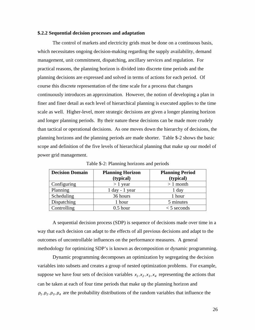
planning horizons and the planning periods are made shorter. Table $-2 shows the basic

scope and definition of the five levels of hierarchical planning that make up our model of

power grid management.

Table $-2: Planning horizons and periods

Decision Domain Planning Horizon (typical)

Planning Period (typical)

Configuring > 1 year > 1 month Planning 1 day - 1 year 1 day Scheduling 36 hours 1 hour Dispatching 1 hour 5 minutes Controlling 0.5 hour < 5 seconds

A sequential decision process (SDP) is sequence of decisions made over time in a

way that each decision can adapt to the effects of all previous decisions and adapt to the

outcomes of uncontrollable influences on the performance measures. A general

methodology for optimizing SDP’s is known as decomposition or dynamic programming.

Dynamic programming decomposes an optimization by segregating the decision

variables into subsets and creates a group of nested optimization problems. For example,

suppose we have four sets of decision variables 4321 x,x,x,x representing the actions that

can be taken at each of four time periods that make up the planning horizon and

4321 p,p,p,p are the probability distributions of the random variables that influence the

27

performance measures of the system that is to be controlled. Each performance measure

may be expressed in terms of some measure of risk with respect to these random

influences. The decision model for optimizing the plan can be stated, )p,p,p,p;x,x,x,x(fmax 43214321

subject to:

0)p,p,p,p;x,x,x,x(g...

0)p,p,p,p;x,x,x,x(g0)p,p,p,p;x,x,x,x(g

43214321n

432143212

432143211

≤

≤

≤

The dynamic programming methodology transforms this optimization into a

nested sequence of optimization problems with the decisions of later time periods nested

with the decisions of earlier time periods. The optimization procedure starts with the

innermost nested problem (last time period) and works in stages to the outermost problem

(first time period). A dynamic programming formulation of the problem described above

is built from the following nested set of optimizations,

⎟⎟⎠

⎞⎜⎜⎝

⎛⎟⎟⎠

⎞⎜⎜⎝

⎛⎟⎠⎞

⎜⎝⎛ )p,p,p,p;x,x,x,x(fmaxmaxmaxmax 43214321xxxx 4321

At each stage, the optimization procedure derives optimal decision rules as

opposed to optimal decisions. A decision rule is a set of contingency-based decisions. In

this case, the contingencies at any stage are the combined effects of all outer decisions

(not yet determined by the optimization procedure) as well as the range of uncontrollable

influences on the performance measures over the time periods prior to the stage’s

decision. Through this methodology we can explicitly express the decision rule for each

time period in terms of the outcomes of the random variables of all previous periods.

Such a representation of the decision rule accurately portrays the real situation that is

faced by the decision maker in each time period.

The correct solution to a stochastic, sequential decision process consists of the

state-contingent decision rules generated by the dynamic programming solution.

However, the derivation of the large number of such decision rules that would be

necessary for a problem as complex as that of unit commitment and dispatch precludes

28

the use of dynamic programming. Instead, planning for stochastic load and generation

levels is achieved through the use of a control heuristic known as rolling horizon and

adaptation. This procedure is used commonly in the commitment and dispatching of

generation units.

Rolling horizon and adaptive control is executed through the combination of three

planning techniques:

• Rolling the plan: Plans are updated at regular intervals. The time between updates

is called the planning interval.

• Planning over a horizon: Each plan extends over a number of future time periods.

The time over which a plan is derived called the planning horizon.

• Adapting the plan: At each update of the plan, the plan is adjusted within limits that

are determined by the system’s constraints on the rates at which resource flows can

change. The planning horizon for each plan consists of a horizon over which the

plan must be “frozen” followed by a horizon over which adjustments are allowed.

The boundary between the fixed portion of a plan and the adjustable portion of a

plan is called the planning “fence”.

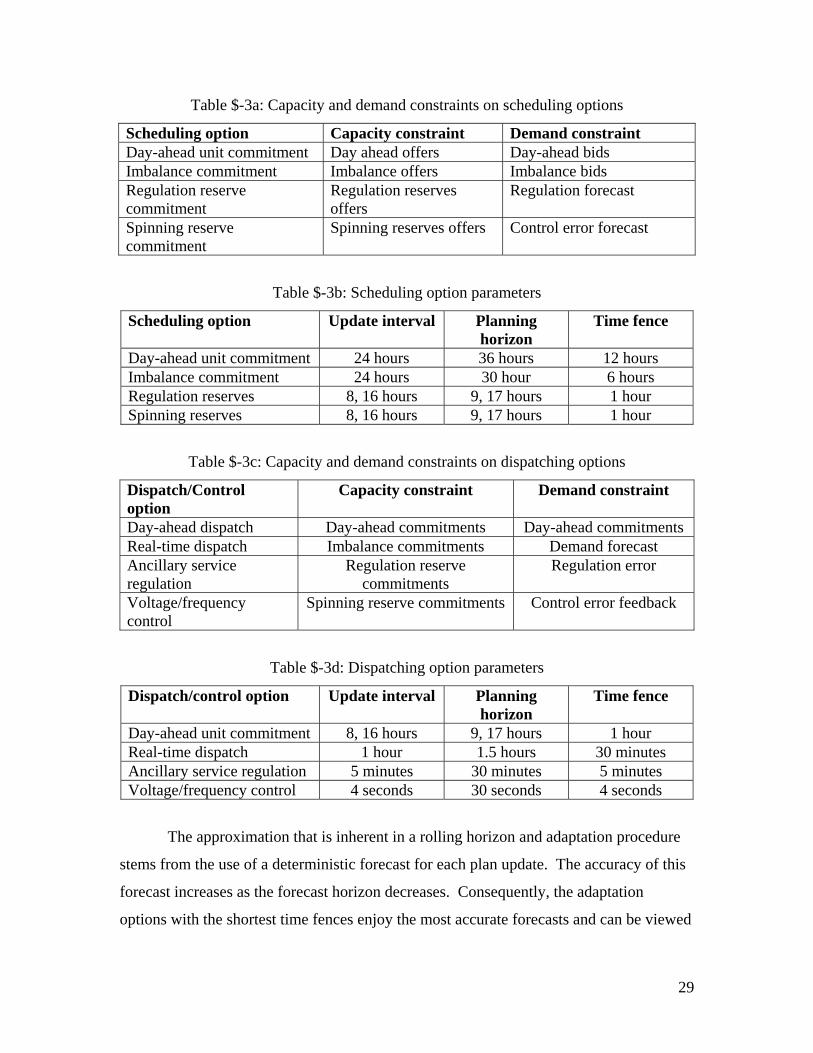
In the case of electricity scheduling and dispatch there are four adaptation options.

Table $-3 defines these options. Each option is constrained to be exercised within the

capacities that are set by the capacity reservation decisions made at a higher level of the

decision-making hierarchy (see previous section). The update intervals, planning

horizons and time fences given in Table $-3 are typical values in the operation of a large

power grid.

29

Table $-3a: Capacity and demand constraints on scheduling options

Scheduling option Capacity constraint Demand constraint Day-ahead unit commitment Day ahead offers Day-ahead bids Imbalance commitment Imbalance offers Imbalance bids Regulation reserve commitment

Regulation reserves offers

Regulation forecast

Spinning reserve commitment

Spinning reserves offers Control error forecast

Table $-3b: Scheduling option parameters

Scheduling option Update interval Planning horizon

Time fence

Day-ahead unit commitment 24 hours 36 hours 12 hours Imbalance commitment 24 hours 30 hour 6 hours Regulation reserves 8, 16 hours 9, 17 hours 1 hour Spinning reserves 8, 16 hours 9, 17 hours 1 hour

Table $-3c: Capacity and demand constraints on dispatching options

Dispatch/Control option

Capacity constraint Demand constraint

Day-ahead dispatch Day-ahead commitments Day-ahead commitments Real-time dispatch Imbalance commitments Demand forecast Ancillary service regulation

Regulation reserve commitments

Regulation error

Voltage/frequency control

Spinning reserve commitments Control error feedback

Table $-3d: Dispatching option parameters

Dispatch/control option Update interval Planning horizon

Time fence

Day-ahead unit commitment 8, 16 hours 9, 17 hours 1 hour Real-time dispatch 1 hour 1.5 hours 30 minutes Ancillary service regulation 5 minutes 30 minutes 5 minutes Voltage/frequency control 4 seconds 30 seconds 4 seconds

The approximation that is inherent in a rolling horizon and adaptation procedure

stems from the use of a deterministic forecast for each plan update. The accuracy of this

forecast increases as the forecast horizon decreases. Consequently, the adaptation

options with the shortest time fences enjoy the most accurate forecasts and can be viewed

30

as “fine tuning” actions with respect to the “coarse tuning” of the plans produced by the

longer-fence options.

$.2.3 Stochastic decisions and risk modeling

Demand for electricity and, to a lesser degree, supply, are not known with

complete certainty, a priori. For this reason, decisions regarding supply availability,

demand management, unit commitment, dispatching, ancillary services and regulation

involve some risk. Such decisions are labeled stochastic. There are several approaches

to coping with risk, all of which incorporate some combination of buffering and

adaptation.

In our model we use a measure of financial risk known as value-at-risk (VAR).

For every business decision, the decision maker has some desired level of financial

performance that is considered satisfactory. However, due to the uncertainties of the real

world, the financial performance of any decision is a random variable that can take on a

range of values with probabilities given by a distribution that is known through the

modeling of the decision. Ranking all of the scenarios for this random variable according

to their associated financial performances, the decision maker can apply his/her own

perspective on risk by specifying a probability that identifies the portion of these

scenarios that constitute the “downside” risk of the decision. For example, a decision

maker could consider the lowest-performing 10% of scenarios as the downside potential

of a decision. Once this probability is set, the minimum financial loss that the downside

scenarios can generate, measured relative to the pre-defined satisfactory level of return, is

called the value-at-risk. VAR is typically computed over a risk horizon of one day and

suffices to represent the exposure of a portfolio of contracts to downside risk from falling

prices or falling demand. Figure $-8 illustrates the concept of VAR.

31

VAR

0 10 20 30 40 50 60 70 80 90 100ReturnSatisfactory

Return

VAR

10%

Figure $-8: Value-at-Risk Example

Mathematically, pursuing the minimization of VAR or constraining VAR below

some tolerable limit is equivalent to adopting the key performance indicator of the

cumulative probability of returns as we prove below.

=V satisfactory return

=C actual cash flow

=−CV financial loss

=α risk level

=L tolerable loss

=CF cumulative distribution of cash flow

=− − )(FV 1C α value at risk

The constraint on VAR is,

L)(FV 1C ≤− − α

which can be expressed more simply as,

32

α≤− )LV(Fc

Risk measures have received much research attention over the last several

decades and this brief discussion of VAR does not do justice to the depth of understanding

of the nature of risk that this research has revealed. The interested reader is referred to

Smithson (1998).

$.2.4 Group decision making and markets

In a regulated power industry, the reservation, commitment and dispatching

decisions are made by a single authorized manager of the power grid. In the case of a

single decision-making authority a decision can be modeled with a single objective

function and accompanying constraints. However, in the case of partially regulated

power grid, supply-availability decisions and demand-management decisions involve

numerous decision makers, each pursuing his/her own self interests. Hence, markets are

born and the decision models that describe the choices of market participants must

recognize the different objectives and constraints of each market participant.

We model each market with a hierarchy of decision models in which capacity

reservations are achieved in the form of bids and offers that are entered into each market

by load-serving entities and suppliers of electricity, respectively. The grid operator then

executes the commitment and dispatching decisions by clearing the markets, which sets

the market clearing prices at each basis point in such a way that all demand constraints

are met and the total cost of power to the entire grid is minimized. Table $-4 lists the

markets that typically drive the management of the grid.

33

Table $-4a: Wholesale Markets Market Transaction Price Buyer Seller Delivery

Node LTC Bi-lateral contract

Bi-lateral contract Bi-lateral Bi-lateral

ISO/DSO LSE

IOU/SA ISO/DSO

Gen bus Load bus

Day-ahead Unit commitment Load commitment

LMP LMP

ISO/DSO LSE

IOU/SA ISO/DSO

Gen bus Load bus

Imbalance Unit dispatch Load dispatch

Real-time LMP

ISO/DSO LSE

IOU/SA ISO/DSO

Gen bus Load bus

Regulation AS

Operating reserves Ancillary service

Real-time LMP

ISO/DSO LSE

IOU/SA ISO/DSO

Gen bus Load bus

Spinning AS

Reserve allocation Ancillary service

Reserve LMP

ISO/DSO LSE

IOU/SA ISO/DSO

Gen bus Load bus

Table $-4b: Retail Markets

Market Transaction Price Buyer Seller Delivery Node

Bi-lateral, Regulated

Long-term contract

Bi-lateral Consumer LSE Load bus

AS = ancillary services

DSO = distribution service operator, distribution grid manager

IOU = investor owned utility

ISO = independent service operator, grid manager

LMP = locational marginal price

LSE = load serving entity or load aggregator

SA = supply aggregator

$.2.5 Power system simulation objects

A simulation of a power system, which portrays the behavior of the system hour-

by-hour over a period of many days, must mimic the behavior of the power grid’s

hardware as well as the decision-making of the customers, suppliers and grid operators

who collectively manage the power system. In order to execute the simulated actions of

market bidding/offering, unit commitment and unit dispatch in the same sequence with

which these actions take place in the real system, a computer simulation of must contain

software objects that behave as the decision-making agents and the grid controllers. In

this section we describe the objects that form the building blocks of a typical power-grid

34

simulation. Specifically, we present the design of a simulation package called the

Virginia Tech Electricity Grid and Market Simulator (VTEGMS). Figure $-9 shows a

flow chart of the interactions of these objects within VTEGMS.

DA Offers and Bids

Buyers and Sellers Data

VTEGMS DFD level 3

3.4.2 DA Market Maker

Submits bids and offers for day-ahead commitment planner

3.4.3 Imbalance Market Maker

Submits bids and offers for hour-ahead commitment

3.4.4 DA Commitment Planner

Prepares DA schedule

3.4.5 Imbalance commitment planner

Prepares hourly schedule

3.4.6 Load Flow Solver

Solves circuit constraints for real and reactive power, voltages

Imb Offers and Bids

Generation and Load Commitment

Generator Data

Load Data

Load Forecast

3.4.1 LoadSim

Randomized load simulator

Bi-lateral contracts

Figure $-9: Simulation of grid-driving decisions

35

$.3 Grid operation models and methods

In this section we describe the models and optimization methods that are used in

VTEGMS, which are also typical of any EGMS. The reader should refer to Figure $-9 to

see how each of the each of the models described in this section is integrated into the

EGMS.

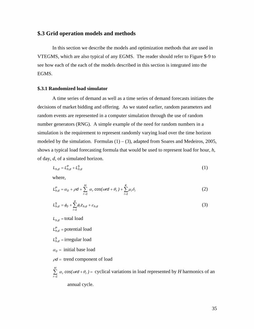
$.3.1 Randomized load simulator

A time series of demand as well as a time series of demand forecasts initiates the

decisions of market bidding and offering. As we stated earlier, random parameters and

random events are represented in a computer simulation through the use of random

number generators (RNG). A simple example of the need for random numbers in a

simulation is the requirement to represent randomly varying load over the time horizon

modeled by the simulation. Formulas (1) – (3), adapted from Soares and Medeiros, 2005,

shows a typical load forecasting formula that would be used to represent load for hour, h,

of day, d, of a simulated horizon. S

d,hP

d,hd,h LLL += (1)

where,

∑∑==

++++=K

1iiirr

H

1r0

Pd,h )rdcos(dL δμθωαρα (2)

∑=

++=p

1id,hd,hi0

Sd,h zL εφφ (3)

=d,hL total load

=Pd,hL potential load

=Sd,hL irregular load

=0α initial base load

=dρ trend component of load

=+∑=

)rdcos( rr

H

1rθωα cyclical variations in load represented by H harmonics of an

annual cycle.

36

=∑=

K

1iiiδμ load adjustments for the day of the week, holidays, etc.

∑=

=+p

1id,hi0 zφφ autoregressive components of load

=d,hε random component of load assumed to be normally distributed with a mean

of zero and a standard deviation of d,hσ

For any day, d, and hour, h, all of the terms in these formulas except d,hε would

be known parameters that the modeler would enter into the simulation program’s

database. The random component of load must be represented in the simulation program

as a different value each time the load for day, d, and hour, h, is simulated. In order to do

this, the simulation program generates a stream of numbers that have the properties of

random drawings of numbers from a normal distribution with a mean of zero and a

standard deviation of d,hσ .

A RNG is a computer program that can produce a stream of numbers that appear

to have come from a specified probability distribution. These streams are actually

computed deterministically by a recursion formula so they are more appropriately called

pseudo-random numbers. However, pseudo-random numbers have all of the statistical

properties of numbers that are randomly generated from a physical process as well as

some non-random properties that make them very useful for simulation studies. The

essential properties of RNG’s are as follows:

1. RNG’s generate numbers that are uniformly distributed between 0 and 1. A

uniformly distributed stream of numbers can be transformed into a stream of

numbers that appear to come from any other probability distribution through

standard computational techniques.

2. Each number generated in a stream of numbers should be statistically independent

of all numbers generated previously and independent of all numbers to be

generated afterwards. This ensures that we are not instilling unwanted memory

into the behavior of the simulated system.

3. A stream of random numbers should be reproducible. This allows one to perform

multiple simulations runs in the context of a simulation experiment in which all

37

factors, including the random influences, are controlled except those that we wish

to change for the sake of the experiment.

4. The computer program that generates the random numbers should be efficient in

terms of computing time and data storage requirements.

Pseudo-random numbers are not truly random. They have a "period" or "cycle

length" so that a stream of pseudo-random numbers will at some point repeat itself. The

pseudo-random number generators embodied in simulation models are constructed so that

the length of the period is very long, alleviating concern about this property causing the

numbers to be dependent on one another.

The pseudo-random numbers are generated by a deterministic formula. This

makes them well-defined and also gives them the reproducibility property that we desire.

The linear congruential method, which we describe in its simplest form below, is the

most common method for generating pseudorandom numbers in the interval [0,1).

Consider a stream of numbers ,.......x,x 10 such that,

( )

seed

=

=

+=

++

+

0

1i1i

i1i

xc

xr

cmodbaxx

a, b, and c are chosen in order to give the stream the longest period possible. For

example, let w = the number of bits/word on the computer used to generate the random

numbers. Then,

c = 2w

b is relatively prime to c

a = 1+4k where k is an integer

Once a stream of pseudo-random numbers in the interval [0,1) are generated they can be

translated into a stream of numbers that appear to have been drawn from any specified

probability distribution such as the normal distribution of mean 0 and standard deviation

d,hσ in the load-forecasting example described earlier. Although it is beyond the scope

of the treatment of simulation offered in this chapter, this transformation is

straightforward and is easily coded into a simulation software package.

38

The interested reader is referred to Banks, et. al. (2005) for more information

about the structure of simulation programs and simulation modeling. Amelin (2004)

provides an overview of simulation models specifically for modeling electricity markets.

$.3.2 Market maker

Following the hierarchy of decisions, we model the planning decisions in terms of

the market strategies of buyers and sellers. In the day-ahead and imbalance wholesale

markets, each supply aggregator offers generation capacity in the form of a “stack”,

which is a list of ordered pairs of power quantities and associated offer prices. When the

market clears, any power that was offered at or below the market clearing price will be

sold by the supply aggregator at the market clearing price. Similarly, each load

aggregator bids on power in the form of a stack in terms of power quantities and

associated bid prices. When the market clears, any power that was bid at or above the

market clearing price will be purchased by the load aggregator at the market clearing

price.

The market maker object of the simulation applies the auction rules described

above for determining the optimal offer and bid functions of each player in the market.

That is, for the simulation of a power market associated with a particular power grid we

construct an instance of the market for each buyer and seller of power and for each type

of energy auction. In order to specify these instances, we define the following notation.

=m market identification = ltc (long term, bi-lateral contract), da (day-ahead

wholesale), imb (imbalance, wholesale), reg (regulation reserve), con

(control reserve)

=mzM market clearing price for zone z in market m

=mzM price cap for m

zM

=mzM price floor for m

zM

=)k(z zone to which generator or load element k belongs

=mkjB jth bid price for power in market m from load element k

=mkjO jth offer price for power in market m from generator k

=GS set of all generator circuit branches

39

=AS set of all transmission lines

=SS set of supply aggregators

=LS set of load aggregators

=GnS the set of generators marketed by supply aggregator n

=LnS the set of loads represented by load aggregator n

=BS the set of all busses

=mkjP jth power segment bid or offered in market m at load or generator element k

mkP new power-commitment in market m in the planning period at load or

generator element k

Market Model for Availability Planning (m = da, rt) for each SSn∈

( ){ } [ ]kSkSk|P,O

REMaxGnGn

mkj

mkj

∑∈∈

Subject to:

nnSk

k VRobPrGn

α<⎟⎟⎠

⎞⎜⎜⎝

⎛<∑

∈

where m

km

)k(zk PMR =

∑≤

=m

)k(zmkj MO

mjk

mk PP

Market Model for Demand Planning (m = da, rt) for each LSn∈

( ){ } [ ]kSkSk|P,B

REMinLnGn

mkj

mkj

∑∈∈

Subject to:

nnSk

k VRobPrLn

α<⎟⎟⎠

⎞⎜⎜⎝

⎛>∑

∈

where m

km

)k(zk PMR =

∑≥

=m

)k(zmkj MB

mjk

mk PP

40

Solution method

In this section we propose a simple, generic market model for the simulation

object that represents the decision of an individual market player. This object is then

instantiated in the simulation for each market participant in each market type. We

assume a market for the buying and selling of power over a particular future time period

that we will call the sale period.

=ic the internal capacity, or maximum volume, of an asset that the market player

can offer (bid) for sale (purchase)

=ec the external capacity, or maximum volume, of the asset that the rest of the

market can offer (bid) for sale (purchase) over the sale period

=m the future market clearing price of the asset, a random variable at the time

offers (bids) are made

=m price cap for the market

=m price floor for the market

=mF cumulative distribution function of m

=d maximum demand for the asset over the sale period

The decision that the market player must make is the set of prices at which each

unit of volume will be offered (bid). In effect, each market player presents a supply or

demand function to the market. We define these decisions in terms of distribution

functions,

=)p(ox fraction of the asset’s maximum volume offered at prices p ≤ , i,ex =

=)p(bx fraction of the maximum demand bid at prices p≥ , i,ex =

1)p(o0 x ≤≤

1)p(b0 x ≤≤

Note: )p(o is right continuous and increasing and )p(b is decreasing and left

continuous. Conventional offer and bid mechanisms allow for the presentation of a

“stack” of power to the market. The stack is a finite set of power volumes with

associated prices. ( ){ }n 1iii p,v = . For offers, ∑≤

=pp

ii

v)p(o and for bids, ∑≥

=pp

ii

v)p(b . For the

41

purpose of this model, we assume that )p(oi is continuous and dpdoi is continuous except

at the point of contact with the boundaries of the constraints, 1)p(o0 i ≤≤

In what follows we derive the decision facing an individual power supplier. The

model for an individual power buyer is analogous. The market clears at a price that

matches supply to demand. This condition is expressed as, )p(db)p(oc)p(oc eeii =+

We re-state the market-clearing condition as,

i

eei c

)p(oc)p(db)p(o −=

We define the right-hand side of this expression as the normalized, residual-

demand random process, )p(d . The market-clearing condition is then,

i

ee

c)p(oc)p(db)p(d −

=

)p(d)p(oi =

We note that )p(d is a random process that is decreasing and left-continuous in p

and the market-clearing condition induces a market-clearing price which is a random

variable. That is, the residual demand process is a function of scenarios, Ωω∈ , which

implies that the market-clearing price is also a function of scenarios, )(m ω . The

distribution of market prices can then be expressed in terms of the distribution (forecast)

of residual demand. ( ))p(oF)p(F idm =

Figure $-10 shows an example of an supply function and several scenarios for

residual demand. The intersections of the supply function with the residual demand

functions indicate the scenarios for market-clearing prices.

42

Bid-Offer

0.00

10.00

20.00

30.00

40.00

50.00

60.00

70.00

80.00

90.00

100.00

20 25 30 35 40 45 50 55 60 65 70 75 80 85 90 95

Price

Volu

me

Figure $-10: Example of residual demand scenarios and offer fraction vs. price

When the market clears, the revenue (cost) that is accrued by a seller (buyer) can

be evaluated as )m(omc)m(r ii=

m is a random variable, so r is a random variable.

=rF cumulative distribution function of the cash flow )m(r over the random

variable, m . Note, ( ) ( ))p(oFpF))p(r(F idmr ==

The market player’s key performance indicators are return and risk. The former

measure is evaluated as the expected cash flow,

[ ] ∫∫∫ ===∞ m

m

iidii

m

mmii

0r dm

dmdo))m(o(f)m(mocdF)m(mocrdFrE

In energy markets, risk is most commonly incorporated in the market decisions in

terms of a constraint on value-at-risk.

43

α≤− )LV(Fr

or

α≤∫−LV

0rdF

By the monotonicity of )m(oi , for any policy, io , there is a well-defined market-

clearing price, β , for which LV)(r −=β or )(dc

LV)(oi

i ββ

β =−

= . Note that β is a

function of the policy io . Furthermore, the monotonicity of )m(r implies that the risk

constraint can be written equivalently as, αβ ≤)(Fm

or

αβ

≤∫m

iid dm

dmdo))m(o(f

The risk constraint is incorporated into an objective function with a lagrange

multiplier, μ .

μαμβ

+−= ∫∫m

iid

m

m

iidii dm

dmdo))m(o(fdm

dmdo))m(o(f)m(mocJ

Badinelli (2006) provides an optimal solution for the supply function by using optimal

control theory.

44

$.3.3 The commitment planner

The market maker object is used in the simulation to determine the “stacks” of

generation offers and load demands for each time period. The next stage in the planning

and scheduling hierarchy is that which clears the market and the selects from the

generation and load stacks the power that will be supplied. However, in making this

selection, the currents, voltages, generation, loads and prices must satisfy numerous

constraints. Subject to these constraints, minimizing the total cost of power that is

needed to cover all of the loads is a typical objective function for power pools and grid

operators. See PJM (2003, 2004, 2005). Hence, we have the optimal power flow (OPF)

problem that we must solve at every instance of commitment planning, which can be

formulated approximately in terms of real power and capacity constraints (DC load flow

model) as follows:

=kP maximum allowed total power at load element or generator element k

=kP minimum required total power at load element or generator element k

element k

=kU maximum upward ramp rate of generator element k

=kD maximum downward ramp rate of generator element k

=moC overhead cost of operating the grid for market m

=kλ congestion cost charged to load element k

=ckP total currently committed power in the planning period at load or generator

∑∈

=mkSk

kjck PP , m = ltc

∑∈

+=mkSk

kjltc

kck PPP , m = da

∑∈

++=mkSk

kjdak

ltck

ck PPPP , m = imb

∑∈

+++=mkSk

kjrt

kdak

ltck

ck PPPPP , m = reg

∑∈

++++=mkSk

kjres

krt

kdak

ltck

ck PPPPPP , m = con

45

=busI vector of all external current phasors at each bus – currents injected to the

grid by generators and currents drawn from the grid by loads.

=busY bus admittance matrix constructed from the admittances of all circuit

elements

=busV vector of voltages at all generator and load busses.

Note:

• The index k used in the notation for generators and loads refers to the unique circuit

branch of the generator or load as opposed to the numerical identifier of the generator

or load.

• Bi-lateral contracts can be modeled as bids and offers at the contract price.

• Must-serve loads (from bi-lateral contracts) can be modeled as bids at the price cap.

• Load shaping through the discretionary use of power can be modeled in terms of the

bids.

• Load shaping through the use of islanded DG can be modeled in terms of the bids.

• Must-run generators (from self-scheduled generators) can be modeled as offers at the

price floor.

Problem: OPF (m = ltc, da, imb, reg, con)

∑∈ GSk

mk

mk PMMin

Subject to:

Constraint set 1

kck PP ≥ for all generators, GSk ∈

kck PP ≤ for all generators, GSk ∈

kck

ckk D)1t(PPU −≥−−≥ for all generators, GSk ∈

Constraint set 2 mz

mz

mz MMM ≤≤ for all zones, z

∑≤

=m

)k(zmkj MO

mkj

mk PP for all generators, GSk ∈

∑≥

=m

)k(zmkj MB

mkj

mk PP for all loads, LSk ∈

46

( ) mo

Sk

mk

m)k(z

Sk

mkk

m)k(z CPMPM

GL

≥−+ ∑∑∈∈

λ

Constraint set 3

• Emissions constraints

• Regulatory constraints

• Inventory constraints for storable power generators

Constraint set 4

kk TP ≤ for all lines ASk ∈

Constraint set 5 busbusbus IVY =

maxkk

mink QQQ ≤≤ for all generators, GSk ∈

maxkk

mink VVV ≤≤ for all busses, BSk ∈

maxkk

mink ααα ≤≤ for all busses, BSk ∈

Constraint set 1, expressed in terms of real power, reflect general physical

limitations of generators. Several market constraints, shown in constraint set 2, are

necessary to model the behavior of the auctions that mechanize the day-ahead and

imbalance markets. The last constraint in this set ensures that the power that is actually

bought or sold is that which the market-clearing process selects and that revenues cover

costs.

Constraint set 3 reflects special considerations of a particular power grid.

Constraint set 4 consists of the thermal limits on the power lines of the grid. These

constraints determine the congestion charge, kλ , that is assigned to any load that cannot

obtain power from the cheapest source of generation because of thermal limits on

transmission lines that connect the load to this generation.

Finally, we must enforce the physical laws that govern real and reactive power

within a circuit as well as limits on the phase and voltages of generator outputs. We

assume that all voltages and currents attain their steady-state, forced-response values

during each interval. We do not include transient behavior in the solution. To this end

we impose Kirchoff’s Current Law and Kirchoff’s Voltage Law on all circuit elements,

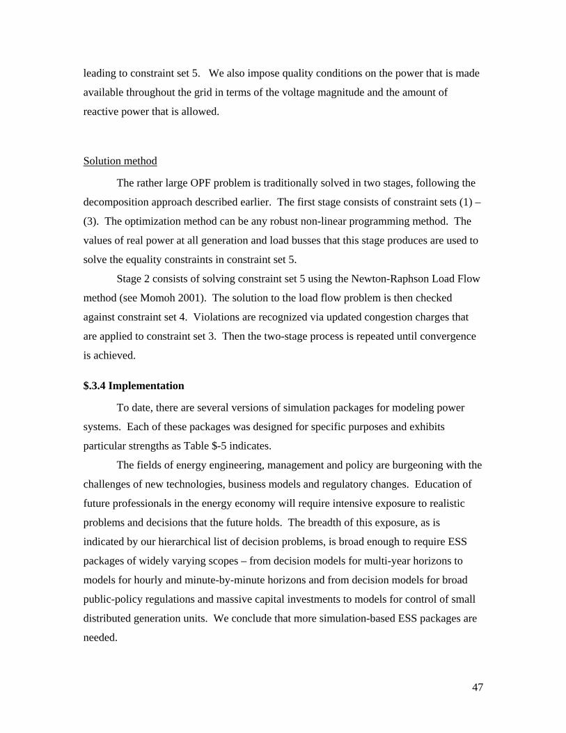
47

leading to constraint set 5. We also impose quality conditions on the power that is made

available throughout the grid in terms of the voltage magnitude and the amount of

reactive power that is allowed.

Solution method

The rather large OPF problem is traditionally solved in two stages, following the

decomposition approach described earlier. The first stage consists of constraint sets (1) –

(3). The optimization method can be any robust non-linear programming method. The

values of real power at all generation and load busses that this stage produces are used to

solve the equality constraints in constraint set 5.

Stage 2 consists of solving constraint set 5 using the Newton-Raphson Load Flow

method (see Momoh 2001). The solution to the load flow problem is then checked

against constraint set 4. Violations are recognized via updated congestion charges that

are applied to constraint set 3. Then the two-stage process is repeated until convergence

is achieved.

$.3.4 Implementation

To date, there are several versions of simulation packages for modeling power

systems. Each of these packages was designed for specific purposes and exhibits

particular strengths as Table $-5 indicates.

The fields of energy engineering, management and policy are burgeoning with the

challenges of new technologies, business models and regulatory changes. Education of

future professionals in the energy economy will require intensive exposure to realistic

problems and decisions that the future holds. The breadth of this exposure, as is

indicated by our hierarchical list of decision problems, is broad enough to require ESS

packages of widely varying scopes – from decision models for multi-year horizons to

models for hourly and minute-by-minute horizons and from decision models for broad

public-policy regulations and massive capital investments to models for control of small

distributed generation units. We conclude that more simulation-based ESS packages are

needed.

48

Table $-5: Comparison of simulation packages

Package Name Creator/Vendor Scope Key Features Applications VTGIS/EGMS

Virginia Tech (Badinelli, et.al. 2005)

Distribution grids & distributed generation

Interfaced with ESRI’s ARCGIS package

Future application in university courses in electrical engineering, business, public policy

GE Maps

General Electric (GE 2005)

Regional grids LMP computation, transmission constraints

Bid strategy, unit commitment, market studies, economic analysis

Aurora

EPIS, Inc. (EPIS 2005)

Regional grids Nodal and zonal LMP computation, transmission constraints

Power flow computation; valuation of generation & transmission assets, FTR’s, LTC’s

SimRen ISUSI (Herbergs et.al. 2005)

Multi-region grids

Dispatches wind, solar, cogen as well as conventional generation

Generation technology selection, installed capacity planning

EMCAS

CEEESA (CEESA 2002)

Adaptive systems model of regional energy markets

Agent-based modeling and simulation

Electricity trading strategies, economic analysis

STEMS EPRI Sort-term markets

Agent-based modeling and simulation

Energy market design, trading strategies

Finally, we emphasize the need for case studies in the education of professionals

in the energy field. Computerized decision support systems alone are useful only to

professionals who already understand the decision problems to which they apply these

systems. However, learners must view each decision problem in a holistic, multi-

disciplinary manner in order to understand fully the tradeoffs inherent in the problem.

Only well-crafted case studies that are supported by companion computerized decision

support systems can impose this view.

49

References

[1] Acha, E., Fuerte-Esquival, C., Ambriz-Perez, H., Angeles-Camacho, C. (2004). FACTS Modelling and Simulation of Power Networks, Jay Wiley & Sons, Ltd.

[2] Amelin, M. (2004). On monte carlo simulation and analysis of electricity markets,

PhD dissertation, Royal Institute of Technology Department of Electrical Engineering, Stockholm.

[3] Badinelli, R. Unit Commitment and Market Strategies for Distributed Generation,

Presentation at National INFORMS meeting, Pittsburgh, November, 2006.

[4] Badinelli, R., Centeno, V., Gregg, M. (2004). A technological tool and case studies for education in the design and management of a secure and efficient distributed generation power system, NSF supplemental grant proposal No. ECS-0323344.

[5] Banks, J., Carson, J., Nelson, B., David, N. (2005). Discrete-event system

simulation 4th Ed., Prentice-Hall.

[6] Barnes, Christensen, and Hansen (1994). Teaching and the Case Method, 3rd Ed., HBS Press.

[7] Bodily, Caraway, Frey, Pfeifer (1998). Quantitative Business Analysis Text and

Cases, McGraw-Hill.

[8] Center for Energy, Economic, and Environmental Systems Analysis (CEEESA) (2002). Electricity markets complex adaptive systems (EMCAS), Argonne National Laboratories, http://www.dis.anl.gov/CEEESA/downloads/emcas_brochure.pdf.

[9] Depablos, J., DeLaRee, J., Centeno, V., “Identifying Distribution Protection

System Vulnerabilities Prompted by the Addition of Distributed Generation, Paper accepted at the CRIS conference on “Protecting Critical Infrastructures”, Grenoble France Oct. 25th to 27th, 2004

[10] EPIS (2005). Auroraxmp® and PowerWorld® Simulator,

http://www.epis.com/Products/OneSheet-APWSI%20050412.pdf.

[11] General Electric (2005). MAPS™ Software, GE, http://www.gepower.com/prod_serv/products/utility_software/en/ge_maps/index.htm.

[12] Grainger, J.J., Stevenson, W.D., (1994). Power Systems Analysis, McGraw-Hill.

[13] Herbergs, S., Lehmann, H., Peter, S. (2005). The computer-modelled simulation

of renewable electricity networks, http://www.susi-

50

con.com/downloads/simren.pdf#search='simulation%20%20electricity', Institute for Sustainable Solutions and Innovations, Aachen, Germany.

[14] Momoh, J.A. (2001). Electric Power System Applications of Optimization,

Marcel Dekker Inc.

[15] PJM, (12/24/2003). Manual #10, Revision 16: Pre-Scheduling Operations

[16] PJM, (12/07/2004). Manual #11, Revision 23: Scheduling Operations

[17] PJM, (01/01/2005). Manual #12, Revision 11: Dispatching Operations

[18] Smithson, C., (1998). Managing Financial Risk, McGraw-Hill.

[19] Soares, L., Medeiros, M. (2005). Modeling and forecasting short-term electricity load: a two-step methodology, working paper No. 495, Department of Economics, Pontifical Catholic University of Rio de Janeiro.

[20] Soman, S., Khaparde, S., Pandit, S. (2002). Computational Methods for Large

Sparse Power Systems Analysis, an Object Oriented Approach, Kluwer Academic Publishers

[21] Wasserman, S. (1994). Introduction to Case Method Teaching. New York:

Teachers College Press.