Embed Size (px)
Citation preview
An-Najah National University Faculty of Graduate Studies
GIS-Based Hydrological Modeling of Semiarid Catchments
(The Case of Faria Catchment)
By
Sameer ‘Mohammad Khairi’ Shhadi Abedel-Kareem
Supervisors
Dr. Hafez Q. Shaheen Dr. Anan F. Jayyousi
Submitted in Partial Fulfillment of the Requirements for the Degree of Master of Science in Water and Environmental Engineering, Faculty of Graduate Studies, at An-Najah National University, Nablus, Palestine
2005
III
بسم الله الرحمن الرحيم
أنزل من السماء ماء فسالت أودية بقدرها فاحتمل السيل
)16(ألرعد .........زبدا رابيا
صدق االله العظيم

IV
… Dedicated to My parents, wife and my daughter (Muna)
V
Acknowledgments
First of all, praise is to Allah for making this thesis possible. I would like to
express my sincere gratitude to Dr. Hafez Shaheen and Dr. Anan Jayyousi
for their supervision, guidance and constructive advice. Special thanks go
also to the defense committee members.
Thanks also go to those who helped in providing the data used in this study.
Water and Environmental Studies Institute or giving me the chance to work
on GLOWA project, Palestinian Water Authority (PWA) for producing of
water data used in this study.
My parents, brothers and sisters, thank you for being a great source of
support and encouragement. All my friends and fellow graduate students,
thank you.
Special thanks to my friend Eng. Rami Qashou’ who’s support will never
be forgotten.
Finally, thanks to my dear wife Heba for her love, moral support and
patience.

VI
Table of Contents ACKNOWLEDGMENTS ........................................................................................................ V TABLE OF CONTENTS ........................................................................................................ VI LIST OF ABBREVIATIONS .......................................................................................... VIII LIST OF TABLES ....................................................................................................................... IX LIST OF FIGURES ...................................................................................................................... X ABSTRACT .................................................................................................................................... XII CHAPTER ONE INTRODUCTION .................................................................................... 1
1.1 BACKGROUND ............................................................................................................................ 2 1.2 OBJECTIVES ................................................................................................................................. 3 1.3 RESEARCH NEEDS AND MOTIVATIONS ....................................................................... 4 1.4 METHODOLOGY ........................................................................................................................ 7 1.5 DATA COLLECTION ................................................................................................................. 9
CHAPTER TWO LITERATURE REVIEW ............................................................... 11
2.1 HYDROLOGY OF SEMIARID REGIONS ........................................................................ 12 2.1.1 Climate and Rainfall ................................................................................................ 13 2.1.2 Runoff Generation and Channel Flow .......................................................... 16 2.1.3 Storages ............................................................................................................................ 17
2.2 RAINFALL-RUNOFF MODELING .................................................................................... 18 2.2.1 Historical Overview ................................................................................................. 19 2.2.2 Classification of Models and Basic Definitions ..................................... 21
2.3 USE OF GIS IN HYDROLOGY .......................................................................................... 23 2.4 PREVIOUS WORK IN THE STUDY AREA .................................................................... 26
CHAPTER THREE DESCRIPTION OF THE STUDY AREA ...................... 28
3.1 LOCATION AND TOPOGRAPHY ....................................................................................... 29 3.2 CLIMATE .................................................................................................................................... 33
3.2.1 Wind ................................................................................................................................... 33 3.2.2 Temperature ................................................................................................................... 34 3.2.3 Relative Humidity ..................................................................................................... 36 3.2.4 Rainfall ............................................................................................................................. 36 3.2.5 Evaporation .................................................................................................................... 38 3.2.6 Aridity of the Catchment ....................................................................................... 40
3.3 WATER RESOURCES ............................................................................................................ 41 3.3.1 Groundwater Wells ................................................................................................... 41 3.3.2 Springs .............................................................................................................................. 42 3.3.3 Analysis of Springs Discharge .......................................................................... 43
3.4 SURFACE WATER .................................................................................................................. 45 3.4.1 Flow Measurements ................................................................................................. 45 3.4.2 Quality Considerations ........................................................................................... 47
VII
3.5 SOIL .............................................................................................................................................. 49 3.6 GEOLOGY ................................................................................................................................... 51 3.7 LAND USE ................................................................................................................................. 53
CHAPTER FOUR RAINFALL ANALYSIS ................................................................ 58
4.1 RAINFALL STATIONS ........................................................................................................... 59 4.2 CATCHMENT RAINFALL .................................................................................................... 60
4.2.1 Density of Rain Gauges ......................................................................................... 60 4.2.2 Consistency of Rainfall Data .............................................................................. 62 4.2.3 Monthly Rainfall ........................................................................................................ 63 4.2.4 Annual Rainfall ........................................................................................................... 66 4.2.5 Trend Analysis ............................................................................................................. 68
4.3 EXTREME VALUE DISTRIBUTION ................................................................................. 71 4.3.1 Gumbel Distribution ................................................................................................ 72
4.4 AREAL RAINFALL ................................................................................................................. 75 4.5 CORRELATION ANALYSIS BETWEEN STATIONS ................................................... 77
CHAPTER FIVE RUNOFF MODELING ..................................................................... 79
5.1 INTRODUCTION ....................................................................................................................... 80 5.2 GIUH MODEL ......................................................................................................................... 81 5.3 TRAVEL TIME ESTIMATION OF THE KW-GIUH MODEL ............................... 83 5.4 STRUCTURE OF THE KW-GIUH MODEL ................................................................. 87 5.5 KW-GIUH MODEL INPUT PARAMETERS ............................................................... 91
5.5.1 Hydraulic parameters .............................................................................................. 91 5.5.2 Geomorphic parameters ......................................................................................... 91 5.5.3 Parameter Estimation Using GIS ..................................................................... 92
5.6 KW-GIUH UNIT HYDROGRAPH DERIVATION .................................................... 97 5.7 SENSITIVITY ANALYSIS ..................................................................................................... 99 5.8 MODEL APPLICATION FOR HYDROGRAPH SIMULATION ............................. 102
5.8.1 Event 1, 14-2-2004................................................................................................. 103 5.8.2 Event 2, 5-2-2005 ................................................................................................... 106
5.9 ANALYSIS AND DISCUSSION ........................................................................................ 108 CHAPTER SIX CONCLUSIONS AND RECOMMENDATIONS .............. 111
6.1 CONCLUSIONS ...................................................................................................................... 112 6.2 RECOMMENDATIONS ........................................................................................................ 114
REFERENCES ............................................................................................................................. 117 APPENDIX A (TABLES) ..................................................................................................... 125 APPENDIX B (FIGURES) .................................................................................................. 162 APPENDIX C (KW-GIUH OUTPUTS) .................................................................... 171 APPENDIX D (PICTURES) .............................................................................................. 179 ب ......................................................................................................................................................... الملخص

VIII
List of Abbreviations Symbol The meaning
KW-GIUH Kinematic Wave based Geomorphological Instantaneous Unit Hydrograph
GIS Geographical Information System DEM Digital Elevation Model EAB Eastern Aquifer Basin PHG Palestinian Hydrology Group PWA Palestinian Water Authority IDF Intensity Duration Frequency Curves MOT Meteorological Office of Transport WESI Water and Environmental Studies Institute N Optimal number of stations Ep Allowable percentage of error Cv Coefficient of variation
avP Mean of rainfall 1−nσ Standard deviation
P(x) Probability of exceedance oixT Time for the flow to reach equilibrium ioq ith-order overland flow discharge per unit width
Lq Lateral flow rate iosh ith-order water depth at equilibrium icsQ ith-order channel discharge at equilibrium
rkxT Travel time for the channel storage component
ckxT Travel time for the channel translation component iOAP Ratio of the ith-order overland area to the catchment area
A Total area of the catchment iN ith-order stream number icL ith-order stream length
on Overland flow roughness cn Channel flow roughness
Ai ith-order sub catchment contributing area S io ith-order overland slope S ic ith-order channel slope
ji xxP Stream network transitional probability ΩB Channel width at catchment outlet
Ω Stream network order
IX
List of Tables Table 1: Abstraction from Wells in the Faria Catchment ........................... 42 Table 2: Spring Groups and Spring Information within Faria catchment .. 43 Table 3: Surface Water Quality Parameters for Badan and Faria Streams . 49 Table 4: Major Soil Types and Characteristics in Faria Catchment ........... 50 Table 5: Total Land use Cover of the Faria Catchment .............................. 56 Table 6: Available Rainfall Stations within the Faria Catchment .............. 60 Table 7: Monthly Rainfall Totals of Nablus Station (mm) ......................... 65 Table 8: Statistical Measurements of the Annual Rainfall of the Six
Stations of Faria Catchment .......................................................... 67 Table 9: Trend Equations for the 5-years Moving Average of the Six
Stations .......................................................................................... 69 Table 10: t and
1 , 22
nt α− −
with 90% and 95% Confidence Intervals .............. 71
Table 11: Parameters of Gumbel Distribution for the Six Stations of the Faria Catchment .......................................................................... 74
Table 12: Areal Rainfall Using the Thiessen Polygon Method .................. 76 Table 13: Coordinates, Elevations, Rainfall Averages and Estimated
Averages for the Six Stations ...................................................... 79 Table 14: ji xxP For the Three Sub-catchments ............................................ 95 Table 15: KW-GIUH Input Parameters for Al-Badan Sub-catchment ....... 96 Table 16: KW-GIUH Input Parameters for Al-Faria Sub-catchment ......... 96 Table 17: KW-GIUH Input Parameters for Al-Malaqi Sub-catchment ...... 98
X
List of Figures Figure 1: A flow Chart Depicting the General Methodology Followed in
this Study ....................................................................................... 9 Figure 2: Arid Regions around the World (UNESCO, 1984) ..................... 12 Figure 3: Hydrologic Cycle with Global Annual Average Water Balance
(Chow et al., 1988) ...................................................................... 15 Figure 4: Classification of Hydrological Models (Lange, 1999) ................ 23 Figure 5: Location of the Faria Catchment within the West Bank ............. 30 Figure 6: Springs and Wells within the Faria Catchment ........................... 31 Figure 7: Topographic Map of the Faria Catchment .................................. 32 Figure 8: Mean Monthly Temperatures in Nablus and Al-Jiftlik .............. 35 Figure 9: Spatial Distribution of the Mean Annual Temperature in the Faria
Catchment .................................................................................... 35 Figure 10: Rainfall Stations and Rainfall Distribution within the Faria
Catchment .................................................................................. 37 Figure 11: Monthly Rainfall and Potential Evapotranspiration Rates (ETo)
in Nablus and Al-Jiftlik ........................................................... 39 Figure 12: Potential Annual Evapotranspiration Rates in the Faria
Catchment ................................................................................. 40 Figure 13: Average, Maximum and Minimum Monthly Discharge of Total
Springs within Al-Badan Sub-catchment.................................. 44 Figure 14: Average, Maximum and Minimum Monthly Discharge of Total
Springs within Al-Faria Sub-catchment .................................... 45 Figure 15: Soil Types of the Faria Catchment ............................................ 51 Figure 16: Geology Map of the Faria Catchment ....................................... 52 Figure 17: Part of the airphotos of Faria Catchment ................................... 53 Figure 18: The New Land use Map of the Faria Catchment ....................... 57 Figure 19: Double Mass Curve for the Stations of Faria Catchment .......... 63 Figure 20: Mean Monthly Rainfall of the Six Stations of the Faria
Catchment ................................................................................. 64 Figure 21: Monthly Average Rainfall of Nablus Station Plotted As
Averages of Five Years Intervals.............................................. 66 Figure 22: Yearly Rainfall of Nablus Station ............................................. 67 Figure 23: The 5-year Moving Average of Nablus, Beit Dajan and Al-Faria
Stations ...................................................................................... 69 Figure 24: The 5-year Moving Average of Tubas, Taluza and Tammun
Stations ...................................................................................... 69 Figure 25: Gumbel Plots of Annual Rainfall for Nablus Station ................ 74 Figure 26: Gumbel Plots of the Standardized Variable of the Six Stations of
Faria Catchment ........................................................................ 75 Figure 27: Thiessen Polygon Map for the Faria Catchment ....................... 77
XI
Figure 28: Runoff Structure for a second-Order Catchment (Lee and Chang, 2005) ......................................................................................... 84
Figure 29: Surface Flow Paths of A third-Order Catchment (Lee and Chang, 2005) ............................................................................. 90
Figure 30: Digital Elevations Model (DEM) for the Faria Catchment ....... 93 Figure 31: The Three Sub-catchments of the Faria Catchment .................. 94 Figure 32: The Stream Order Networks for the Three Sub-catchments of
the Faria Catchment .................................................................. 95 Figure 33: 1mm-GIUH for Al-Faria and Al-Badan Sub-catchments ......... 99 Figure 34: 1mm-GIUH for Al-Malaqi Sub-catchment ............................... 99 Figure 35: Variation of GIUH with Excess Rainfall ................................... 99 Figure 36: Sensitivity Analysis of Channel Width on GIUH ................... 100 Figure 37: Sensitivity Analysis of Overland Roughness Coefficient on
GIUH ....................................................................................... 101 Figure 38: Sensitivity Analysis of Channel Roughness Coefficient on
GIUH ....................................................................................... 102 Figure 39: Al-Badan Sub-catchment and its Drainage Network .............. 103 Figure 40: Rainfall Depth and Infiltration Capacity Curve of 14/2/2004
Event ........................................................................................ 105 Figure 41: Recorded and Estimated Direct Runoff Hydrograph for Al-
Badan Sub-catchment, Event of 14/2/2004 ............................. 106 Figure 42: Rainfall Depth and the Phi-Index of Event of 5/2/2005 .......... 107 Figure 43: Recorded and Estimated Direct Runoff Hydrograph for Al-
Badan Sub-catchment, Event of 5/2/2005 ............................... 108
XII
GIS-Based Hydrological Modeling of Semiarid Catchments
(The Case of Faria Catchment) By
Sameer ‘Mohammad Khairi’ Shhadi Abedel-Kareem Supervisors
Dr. Hafez Q. Shaheen Dr. Anan F. Jayyousi
Abstract Extreme events, such as severe storms, floods, and droughts are the main
features characterizing the hydrological system of a region. In the West
Bank, which is characterized as semiarid; little work has been carried out
about hydrological modeling. This thesis is an attempt to model the
rainfall-runoff process in Faria catchment, which is considered as one of
the most important catchments of the West Bank. Faria catchment
dominating the north eastern slopes of the West Bank is a catchment of
about 334 km2 and has the semiarid characteristics of the region. The
catchment is gauged by six rainfall stations and two runoff flumes.
Statistical analysis including annual average, standard deviation, maximum
and minimum rainfall was carried out for the rainfall stations. The internal
consistency of rainfall measurements of the six stations was examined by
using the double mass curve technique. The results show that all station
measurements are internally consistent.
Gumbel distribution fits well the annual rainfall and can be used for future
estimations. It provides means to understand and evaluate the distribution
characteristics of the rainfall in the Faria catchment. Trend analysis of the
rainfall has shows an increasing trend for the stations with high elevations
and a decreasing trend for low elevated ones. The multiple regression
analysis applied to the six rainfall stations proved to be strongly correlated.
XIII
GIS-based KW-GIUH hydrological model was used to simulate the
rainfall-runoff process in the Faria catchment. GIUH unit hydrographs
were derived for the three sub-catchments of Faria namely Al-Badan, Al-
Faria and Al-Malaqi. The KW-GIUH model is tested by comparing the
simulated and observed hydrographs of Al-Badan sub-catchment for two
rainstorms with good results. Sensitivity of the KW-GIUH model
parameters was also investigated. The simulated runoff hydrographs proved
that the GIS-based KW-GIUH model is applicable to semiarid regions and
can be used to estimate the unit hydrographs in the West Bank catchments.

1
CHAPTER ONE
INTRODUCTION
2
1.1 Background
Water is the chief ingredient of life and all ancient civilizations flourished
only near the water sources and then probably collapsed when the water
supply failed. Water is a finite resource, essential for agriculture, industry
and human existence. Without water of adequate quantity and quality,
sustainable development is impossible. Water resources management is
essential to ensure the availability of water, when and where it is needed,
and to safeguard its quality.
Hydrologists and water engineers are always concerned with discharge
rates resulting from rainfall. Not only measuring rainfall and the resulting
runoff are of interest, but also the process of transforming the rainfall
hyetograph into runoff hydrograph. Peak flow rate and time to peak are the
two important hydrograph characteristics that need to be estimated for any
catchment. Unfortunately, the classic problem of predicting these
parameters is usually difficult to resolve because many rivers and streams
are ungauged, especially those in developing regions or isolated areas.
Even in cases where catchments are gauged, the period of record is often
too short to allow accurate estimates of the different hydraulic parameters.
Flood frequency analysis enables the user to predict flow rates with certain
return periods. Historical flow data is necessary to conduct such analysis.
Hydrological models that incorporate catchment characteristics to predict
flow rates at a given location in the catchment is another tool to be utilized
in cases where historical flow records are not available.
Hydrological simulation models can take the form of theoretical linkage
between the geomorphology and hydrology. The geomorphological
instantaneous unit hydrograph (GIUH) is one approach of this kind of
3
model. The GIUH focuses on finding the catchment response given its
geomorphological features. The GIUH model is applied in this study to
Faria catchment in the northern West Bank. The model uses catchment
characteristics to predict flow rates.
West Bank is a semiarid region. In arid and semiarid regions storm water
drainage and hydrological modeling is important as in humid regions
because it is not only a drainage problem but also a water resources
management and planning problem. Hydrological modeling in the West
Bank has not been given enough care and no intensive studies have been
done.
In characterizing the catchment, GIS has been applied. Using GIS in
hydrology has become an important issue since the beginning of 1980 and
up to the present. It enables the user to handle and analyze the hydrological
data more efficiently.
This thesis concentrates on modeling the rainfall-runoff process in the
upper part of the Faria catchment in the northern West Bank. GIS-based
KW-GIUH hydrological model was applied as it is available and can model
ungauged catchments. The KW-GIUH model can be applied to any excess
rainfall through convolution to produce the direct runoff hydrograph.
1.2 Objectives
Modeling the runoff in the Faria catchment will provide basic information
for the managers to understand runoff generation within the catchment and
thus support the decision-making process about future development of the
water resources in the area. This will enhance the development of the
4
agricultural sector. It will also support the studies of the Jordan River Basin
as Wadi Faria catchment is a major contribution to the Jordan River.
The main objective of this research is to model the rainfall runoff process
of the Faria catchment and to derive the unit hydrograph for the catchment.
The KW-GIUH model that was developed for ungauged catchments is to
be used in this research. The geomorphological and topographic
characteristics were provided using the GIS system.
The other objectives of this study are:
1. Analysis of rainfall data of the Faria catchment.
2. Investigate the rainfall runoff process in semiarid regions.
1.3 Research Needs and Motivations
Faria catchment is predominantly arid and semiarid characterized by its
natural water resources scarcity, low per capita water allocation and
conflicting demands as well as shared water resources. This scarcity leads
to the limited availability of water resources and the dire need to manage
these resources.
Faria catchment, located in the northeastern part of the West Bank,
Palestine, is one of the most important agricultural areas in the West Bank.
The predominantly rural population in the catchment is growing rapidly,
which results in increasing demand for natural water resources.
The prolonged drought periods in the catchment and the high population
growth rate in addition to other artificial constraints have negatively
affected the existing obtainable surface water and groundwater resources.
5
Due to the fact that the available water resources in the Faria catchment are
limited and are not sufficient to fulfill the agricultural and residential water
demand, reliability assessment of water availability in the Faria catchment
is of great importance in order to optimally manage the local water
resources.
Rural population in the Faria catchment faces a series of problems. These
problems are related to different causes including inefficient management,
water shortages, environmental pollution, and Israeli occupation. The key
problems of the Faria catchment relevant to the water resources can be
summarized as follows:
1. Lack of proper management of water resources causes over
utilization of the scarce water resources.
2. The water is not properly allocated between upstream and
downstream communities and thus water use rights need to be well
established and institutionalized.
3. More than 40% of the people in the catchment lacks water supply for
drinking purposes.
4. The estimated annual water gap between water needs and obtainable
water supply is about 20 millions cubic meters. This gap is
increasing rapidly with time.
5. Lack of storage capacity and non existence of small dams to capture
the rain floods during the rainy season in order to be used later (As to
peace agreements, permits for such projects are required from Israeli
occupation authorities, which are almost impossible to obtain).

6
6. Unbalanced utilization of groundwater causes increasing salinity
especially in the south eastern part of the catchment in the proximity
of the Jordan River.
7. Water losses through evaporation and infiltration from the
agricultural canals are high and thus large quantities of water are not
fully utilized.
8. Soil erosion in the lower part of the catchment is of great concern.
9. Water pollution is an ongoing problem. For instances surface water
originating from the springs mixes with wastewater coming from
Nablus City and Faria refugee camp.
10. There is no treatment plant in the catchment.
11. Cesspools are major threats to pollute the groundwater aquifers and
springs.
12. The unbalanced use of fertilizers and pesticides has led to the
pollution of the scarce water resources.
13. Unmanaged solid waste dumping in some areas adds additional
complexity to the pollution problems.
14. Lack of permits to rehabilitate and remediate the deteriorated wells.
15. In contrast to the shallow Palestinian wells, Israeli wells are pumping
largely from deep aquifers and thus lowering the water table.
From the above it can be inferred that Faria catchment is under a severe
problematic conditions that need to be investigated in order to set up proper
7
strategies and management alternatives to address these problems
efficiently indemnify.
For the aforementioned discussion, this study is of great importance. Due to
the fact that the available water resources in the Faria catchment are limited
and cannot suffice for increasing water demand to fulfill the agricultural
and residential requirements, reliability assessment of water availability in
the Faria catchment is of great importance in order to optimally manage the
local water resources. This situation has compelled the motivation for
conducting a hydrological modeling to better understand and to evaluate
the water resources availability in the Faria catchment. This modeling is
essential to provide input data for a management system and to enable the
development of optimal water allocation policies and management
alternatives to bridge the gap between water needs and obtainable water
supply under drought conditions.
1.4 Methodology
To achieve the above objectives, the available topographic maps of the
region were scanned and the catchment was subdivided into sub-
catchments. Drainage lines and divides were digitized. The stream paths,
possible flow directions and slopes have been determined using the
available Digital Elevation Model (DEM) and the base map of the Faria
catchment has been prepared. All the information including topography,
land use, drainage lines, water divides, soil and geology have been
processed using the GIS ArcView 3.2 software.
The rainfall data recorded by the different stations of the Faria catchment
were analyzed for typical and maximum rainfall intensities and amounts.

8
These were used as a tool to describe the spatial structure of the rain events
and to regionalize point station data to catchment rainfall. Rainfall and
runoff were measured continuously during the rainstorms of the last two
rainy seasons of the hydrological years 2003-2004 and 2004-2005.
Accordingly the input parameters to the KW-GIUH model have been
estimated.
The following summarizes the main steps that were followed:
1. Collect all data and information from national and local institutions.
2. Hydrological measurements and sampling of rainfall-runoff events
completed for the two rainy seasons.
3. Analysis of rainfall and runoff data.
4. Set up GIS-based data as input for the model.
5. Model application to the available different rainfall events.
6. Model verification and sensitivity analysis.
7. The final results of the modeling have been formulated.
The overall methodology followed in this study is illustrated in Figure 1.
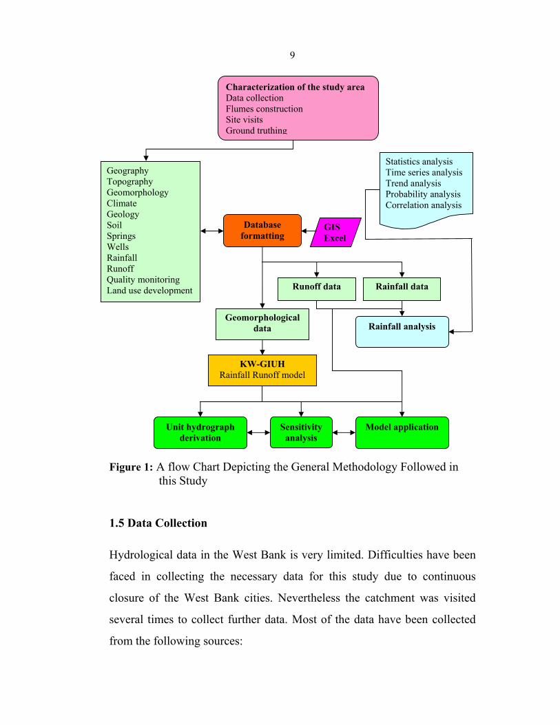
9
Figure 1: A flow Chart Depicting the General Methodology Followed in this Study
1.5 Data Collection
Hydrological data in the West Bank is very limited. Difficulties have been
faced in collecting the necessary data for this study due to continuous
closure of the West Bank cities. Nevertheless the catchment was visited
several times to collect further data. Most of the data have been collected
from the following sources:
KW-GIUH Rainfall Runoff model
Geography Topography Geomorphology Climate Geology Soil Springs Wells Rainfall Runoff Quality monitoring Land use development Runoff data
GIS Excel
Database formatting
Characterization of the study area Data collection Flumes construction Site visits Ground truthing
Statistics analysis Time series analysis Trend analysis Probability analysis Correlation analysis
Unit hydrograph derivation
Rainfall analysis Geomorphological
data
Rainfall data
Sensitivity analysis
Model application
10
1. Contour Map. The available 1:50000 scale topographic maps have
been used to collect elevation data. The maps have been scanned and
used within the GIS environment to delineate the catchment and sub-
catchments boundaries and divides. The stream paths, possible flow
directions and slopes have been determined using the available
Digital Elevation Model (DEM).
2. Water resources (springs and wells) data were obtained from the
Palestinian Water Authority (PWA) databank. The data included
monthly and annual measurements of the abstraction of the wells and
yield of springs in addition to the name and coordinates of these
resources. The information obtained was in MS Excel format.
3. Rainfall data necessary for the analysis of the rainfall-runoff process
have been collected from the PWA and from Nablus Meteorological
Station for five different stations (Taluza, Tammun, Tubas, Beit
Dajan and Al-Faria).
4. The climatic data for this study was obtained from the Palestine
Climate Data Handbook published by the Metrological Office of the
Ministry of Transport (MOT), 1998. Climatic data included average
monthly values for maximum and minimum temperature, hourly
mean wind speed, daily mean sunshine duration, mean relative
humidity, pan evaporation and mean monthly rainfall for Nablus and
Al-Faria stations.

11
CHAPTER TWO
LITERATURE REVIEW
12
2.1 Hydrology of Semiarid Regions
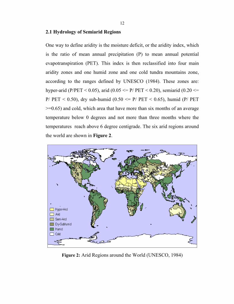
One way to define aridity is the moisture deficit, or the aridity index, which
is the ratio of mean annual precipitation (P) to mean annual potential
evapotranspiration (PET). This index is then reclassified into four main
aridity zones and one humid zone and one cold tundra mountains zone,
according to the ranges defined by UNESCO (1984). These zones are:
hyper-arid (P/PET < 0.05), arid (0.05 <= P/ PET < 0.20), semiarid (0.20 <=
P/ PET < 0.50), dry sub-humid (0.50 <= P/ PET < 0.65), humid (P/ PET
>=0.65) and cold, which area that have more than six months of an average
temperature below 0 degrees and not more than three months where the
temperatures reach above 6 degree centigrade. The six arid regions around
the world are shown in Figure 2.
Figure 2: Arid Regions around the World (UNESCO, 1984)
13
The main hydrological difference between humid areas and arid zones is a
high variability in both space and time of all hydrologic parameters (e.g.
rainfall intensity, infiltration rates, runoff rates). Floods, although
infrequent and rare, appear in arid areas and often cause loss of life and
property (Schick et al, 1997, cited by Thormählen, 2003). Many semiarid
regions are particularly affected by flash floods, caused mainly by
convective storm systems. The main processes that dominate during flashy
floods are the generation of Hortonian overland flow on dryland terrain and
transmission losses into the dry alluvial beds of ephemeral channels. In dry
environments, the hydrological regime is governed by missing baseflow
and single episodic flood events traveling on dry river beds, induced by
localized, high intensity rainfall (Thormählen, 2003).
2.1.1 Climate and Rainfall
The main climatological feature of arid regions is the ephemeral and often
localized nature of precipitation usually associated with immense variations
in space and time (Thormählen, 2003). The arid zone is characterized by
excessive heat and inadequate variable precipitation; however, contrasts in
climate occur. In general, these climatic contrasts result from differences in
temperature, the season in which rain falls, and in the degree of aridity.
Three major types of climate are distinguished when describing the arid
zone: the Mediterranean climate, the tropical climate and the continental
climate (FAO, 1989).
In the Mediterranean climate, the rainy season is during autumn and winter.
Summers are hot with no rains; winter temperatures are mild, with a wet
season starting in October and ending in April or May, followed by 5 to 6
months of dry season.

14
In the tropical climate, rainfall occurs during the summer. Winters are long
and dry. In Sennar, Sudan, an area that is typical of the tropical climate, the
wet season extends from the middle of June until the end of September,
followed by a dry season of almost 9 months.
In the continental climate, the rainfall is distributed evenly throughout the
year, although there is a tendency toward greater summer precipitation. In
Alice Springs, Australia, each monthly precipitation is less than twice
corresponding mean monthly temperature; hence, the dry season extends
over the whole year.
The rainfall that falls is either intercepted by trees, shrubs, and other
vegetation, or it strikes the ground surface and becomes overland flow,
subsurface flow, and groundwater flow. Regardless of its deposition, much
of the rainfall eventually is returned to the atmosphere by
evapotranspiration processes from the vegetation and soil or by evaporation
from streams and other bodies of water into which overland, subsurface,
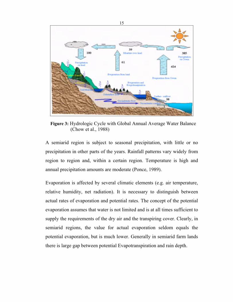
and groundwater flow move. These processes are as illustrated by the
hydrologic cycle in Figure 3, in which global annual average water
balances are given in units relative to a value of 100 for the rate of
precipitation on land.
Rainfall intensity is another parameter which must be considered when
evaluating the rainfall runoff process. Because the soil may not be able to
absorb all the water during a heavy rainfall, water may be lost by runoff.
Likewise, the water from a rain of low intensity can be lost due to
evaporation, particularly if it falls on a dry surface.
15
Figure 3: Hydrologic Cycle with Global Annual Average Water Balance (Chow et al., 1988)
A semiarid region is subject to seasonal precipitation, with little or no
precipitation in other parts of the years. Rainfall patterns vary widely from
region to region and, within a certain region. Temperature is high and
annual precipitation amounts are moderate (Ponce, 1989).
Evaporation is affected by several climatic elements (e.g. air temperature,
relative humidity, net radiation). It is necessary to distinguish between
actual rates of evaporation and potential rates. The concept of the potential
evaporation assumes that water is not limited and is at all times sufficient to
supply the requirements of the dry air and the transpiring cover. Clearly, in
semiarid regions, the value for actual evaporation seldom equals the
potential evaporation, but is much lower. Generally in semiarid farm lands
there is large gap between potential Evapotranspiration and rain depth.
16
2.1.2 Runoff Generation and Channel Flow
The high variability of rainfall both in time and space, leads to very high
variability of runoff. In humid regions different runoff generation processes
(e.g. runoff from saturated areas and slow outflow of large groundwater
bodies) deliver more or less permanently water to perennial rivers. In
contrast, in arid regions Hortonian overland flow, generated as infiltration
excess runoff, is generally assumed to be the dominant mechanism of
runoff generation (Abrahams et. al, 1994). The overland flow is described
as water that flows over the ground surface heading for the next stream
channel and as the initial phase of surface runoff in arid environments
(Lange et al., 2003). On plane surfaces a quasi laminar sheet flow may
develop, but, more usually, flow is concentrated by topographic
irregularities and water flows anatomizing in small gullies and minor
rivulets downhill. The main cause of overland flow is the inability of water
to infiltrate the surface as a result of high intensity of rainfall or a low value
of infiltration capacity or both phenomena (Thormählen, 2003). The
difference between rainfall rate and infiltration rate is the concept of
calculation the runoff of Hortonian overland flow. Water accumulates on
the top of the ground surface, if the infiltration capacity of the soil is
exceeded. Surface depressions have to be filled with water, after that
runoff generation start to runs down slope. Arid areas with moderate to
steep slopes and sparse vegetation cover form the ideal conditions for
Hortonian runoff.
Streams in the arid and semiarid areas are usually ephemeral, since rainfall
events are seldom occurred. Arid and semiarid ephemeral streams flowing
only occasionally as a direct response to runoff generating rainstorms and
remaining dry for most of the year. Flow in the large streams with their
17
origin outside the arid zone (e.g. Nile River, Indus River or Colorado
River) and small spring fed streams are the only exceptions (Thormählen,
2003). Floods in small dryland basins are usually of the flash flood type,
either single peak floods or multiple peak events. Flash floods are almost
produced by convective rain storm cells and are typical for small scale
catchments (<100km²), because most thunderstorm cells are relatively
small in diameter. Flash floods are defined as stream flows that increase
from zero to a maximum within a few minutes or at most few hours (Graf,
1988).
Surface runoff in the eastern slopes of the West Bank where the Faria
catchment is located is mostly intermittent and occurs when rainfall
exceeds 50 mm in one day or 70 mm in two consecutive days (Forward,
1998, cited by Takruri, 2003). Rofe and Raffety (1965) studied runoff in
the West Bank through monitoring and studying runoff data from
seventeen flow gauging stations within the boundaries of the West Bank.
They concluded that surface runoff constitute nearly 2.2% of its total
equivalent rainfall.
2.1.3 Storages
Two types of surface flow losses occur in the arid lands, which fill
temporal storages (Lange, 1999):
1. Infiltration is a direct loss with Hortonian runoff that governs the
volume of storm runoff. Further direct losses occur when water is
temporarily stored on route or in the stream system as detention loss
or when depression storages retain water in depressions on the
surface.
18
2. Linear transmission losses into the riverbed alluvium of the stream
channels reduce flood volume as indirect losses, after surface flow
has been generated and flows spatially concentrated.
The main water storage in dry environments is formed by coarse river bed
alluvium. With rainfall events broadly separated in time, the alluvial fill has
a large available volume for flood water infiltration practically at all times.
The alluvial storages form an infiltration trap for water that flows into them
either through the orderly tributary system or directly from adjoining slopes.
The alluvial bodies, filled by indirect losses may be relatively permanent
and quite deep, serving as important water storage for vegetation or local
population. Compared to alluvial fills, the second type of storage is
shallower. It is recharged by direct losses and is quickly emptied by
evaporation within a few days after the rainfall event. Percolation from
rainfall to deep aquifers is generally very small.
2.2 Rainfall-Runoff Modeling
The selection, analysis and use of recorded hydrographs for direct
simulation purposes are reflected in variation of the unit hydrograph
technique. This technique, which assumes a linearity of the transfer
function, is computationally attractive and often sufficiently accurate. Unit
hydrograph techniques may be applied to synthesize hydrographs either
from recorded rainfall events or from specific return period storms
extracted from intensity-duration-return period curves and hypothetical
time duration patterns (Chow et al., 1988). Hydrological modeling is
concerned with the accurate prediction of the partitioning of water among
the various pathways of the hydrological cycle (Dooge, 1992 cited by
Lange, 1999). Hydrological systems are generally analyzed by using

19
mathematical models. These models may be empirical or statistical, or
founded on known physical laws. They may be used for such simple
purposes as determining the rate of flow that roadway grate must be
designed to handle, or they may be used to guide decisions about the best
way to develop a river basin for a multiplicity of objectives. The choice of
the model should be tailored to the purpose for which it is to be used. In
general, the simplest model capable of producing information adequate to
deal with the issue should be chosen (Viessman et al., 2003).
Hydrological models are used for several practical purposes. Imagine a
flood disaster; during the flood event a model may help to predict when and
where there is a risk of flooding (e.g., which areas should be evacuated).
After the flood, models may be used to quantify the risk that a flood of
similar or larger magnitude will occur during the coming years and to
decide what measures of flood protection may be needed for the future.
Furthermore, models may help to understand the reasons for the magnitude
of flood (e.g., if the flood was enlarged by human activities in the
catchment) (Lundin et al., 1998).
2.2.1 Historical Overview
The development and application of hydrological models have gone
through a long time period. The origins of rainfall-runoff modeling in the
broad sense can be found in the middle of the 19th century, when
Mulvaney, an Irish engineer who used in the first time the rational equation
to give the peak flow from rainfall intensity data and catchment
characteristics. A major step forward in hydrological analysis was the
concept of the unit hydrograph introduced by Sherman in 1932 on the basis
of superposition principle. The use of unit hydrograph made it possible to
20
calculate not only the flood peak discharge (as the rational method does)
but also the whole hydrograph (the volume of surface runoff produced by
the rainfall event). The real breakthrough came in the 1950s when
hydrologists became aware of system engineering approaches used for the
analysis of complex dynamic systems (Todini, 1988). This was the period
when conceptual linear models originated (Nash, 1958). Many other
approaches to rainfall-runoff modeling were considered in the 1960s. A
large number of conceptual, lumped, rainfall-runoff models appeared
thereafter including the famous Stanford Watershed Model (SWM-IV)
(Crawford and Linsley, 1966) and the HBV model (Bergström and
Forsman, 1973). A great variety of these conceptual hydrological models
has appeared up to the present date. TOPMODEL is one remarkable model
developed in the late 1970s (Beven and Kirkby, 1979) that is based on the
idea that topography exerts a dominant control on flow routing through
upland catchments.
To meet the need of forecasting (1) the effects of land use changes, (2) the
effects of spatially variable inputs and outputs, (3) the movements of
pollutants and sediments, and (4) the hydrological response of ungauged
catchments where no data are available for calibration of a lumped model,
the physically based distributed parameter models were developed. SHE
model is an excellent example of such models (Lange, 1999).
Geomorphological Instantaneous Unit Hydrograph (GIUH) (Rodriguez-
Iturbe and Valdes 1979) is a recently developed physically based rainfall-
runoff approach for the simulation of runoff hydrograph, especially
appropriate for ungauged catchments. Lange 1999 mentioned that GIUH
model has been used by Allam (1990), Nouh (1990) and Al-Turbak (1996)
to develop unit hydrograph for several catchments in the Kingdom of Saudi
21
Arabia. In the semiarid experimental catchment of Walnut Gulch, Arizona,
USA, the long history of research provides good runoff records, which
facilitated the successful application of calibrated models (Goodrich et al.
1997 and Renard et al.1993 cited by Thormählen, 2003). The long history
of research also allowed a non-calibrated model run of KINEROS, a
complex distributed model developed for semiarid catchments
(Thormählen, 2003). Lange et al. (1999) develop a model not depending on
calibration but accounting for the dominant processes of arid zone flood
generation. This has been done for the 1400 km² Zin catchment in the
Nagab Desert. The ZIN-Model has been developed especially for large arid
catchments and has been tested successfully for 250 km² in the semiarid
Wadi Natuf (Lange et al. 2001).
2.2.2 Classification of Models and Basic Definitions
Two types of mathematical models can be used in hydrology; stochastic
and deterministic models. In the stochastic models, the chance of
occurrence of the variable is considered thus introducing the concept of
probability. In the deterministic models, the chance of occurrence of the
variables involved is ignored and the model is considered to follow a
definite law of certainty but not any law of probability (Raghunath, 1985).
Different classification schemes have been proposed (e.g. Chow et al.,
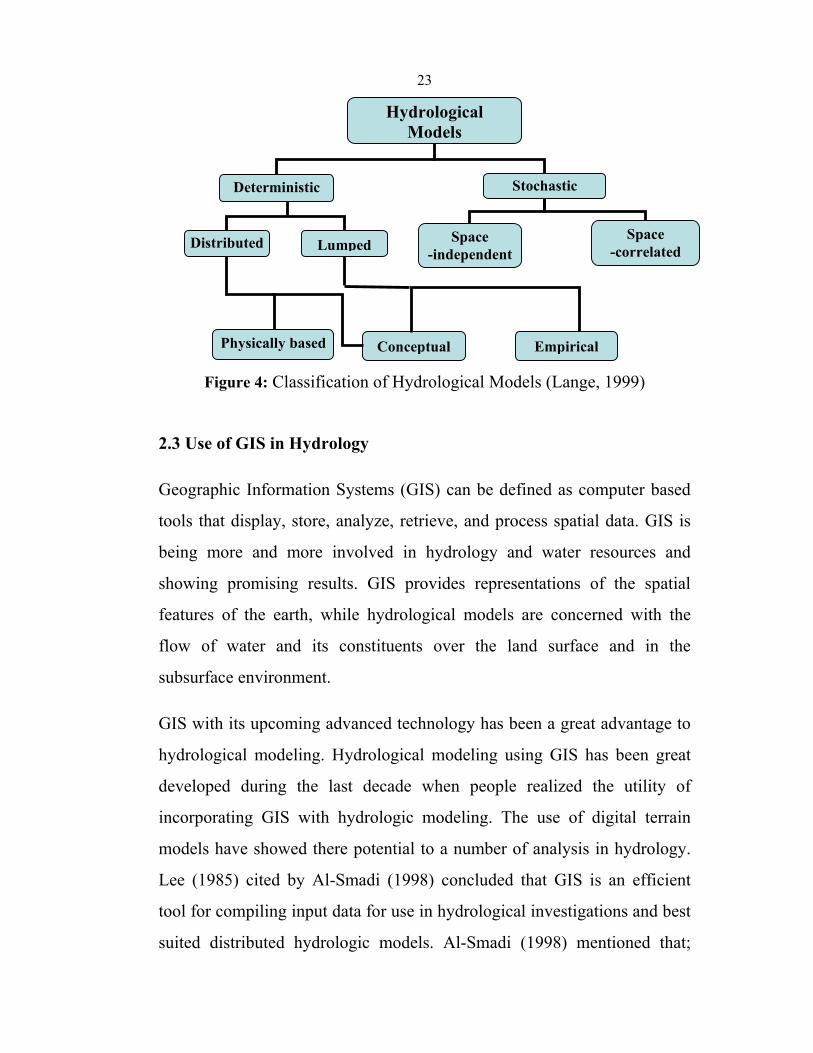
1988, Todini 1988). Figure 4 provide a general overview of the
hydrological model using the classification criteria randomness, spatial
discretization and model structure. To find the desired hydrological model
one should ask the following questions (Lange, 1999):
1- Is there a need to consider randomness?
22
2- Is there a need to consider spatial variations of model input or
parameter?
3- To what extent the governing physical laws have to be considered?
Randomness is not considered in a deterministic model; a given input
rainfall always produces the same output runoff. The outputs of a stochastic
model are at least partially random. A deterministic distributed model
considers the hydrological process taking place at various points in space.
It may either be physically based, i.e. reproducing the rainfall-runoff
process only by physical principals on the conservation of mass and
momentum, or conceptual reflecting these principals in a simplified
approximate manner. In deterministic lumped models hydrological systems
are spatially averaged or regarded as a single point in scale without
dimensions. Since hydrological processes generally are space dependent,
spatial lumping always includes crude conceptualization. Empirical models
do not explicitly consider the governing physical laws of the processes
involved. They only relate input through some empirical transformed
function. Stochastic models are termed space-independent or space-
correlated according to whether or not random variables at different points
in space influence each other.
23
Figure 4: Classification of Hydrological Models (Lange, 1999)
2.3 Use of GIS in Hydrology
Geographic Information Systems (GIS) can be defined as computer based
tools that display, store, analyze, retrieve, and process spatial data. GIS is
being more and more involved in hydrology and water resources and
showing promising results. GIS provides representations of the spatial
features of the earth, while hydrological models are concerned with the
flow of water and its constituents over the land surface and in the
subsurface environment.
GIS with its upcoming advanced technology has been a great advantage to
hydrological modeling. Hydrological modeling using GIS has been great
developed during the last decade when people realized the utility of
incorporating GIS with hydrologic modeling. The use of digital terrain
models have showed there potential to a number of analysis in hydrology.
Lee (1985) cited by Al-Smadi (1998) concluded that GIS is an efficient
tool for compiling input data for use in hydrological investigations and best
suited distributed hydrologic models. Al-Smadi (1998) mentioned that;
Conceptual
Deterministic
Hydrological Models
Stochastic
Space -independent
Space -correlated Distributed
Physically based
Lumped
Empirical
24
Berry and Sailor (1987) noted some of the advantages of GIS in hydrology
and water resources. According to them, GIS provides a powerful tool for
expressing complex spatial relationships. It provides an opportunity to fully
incorporate spatial conditions into hydrologic inquiries. Different proposed
levels of development can be made rapidly and the resulting hydrologic
effects easily communicated to decision makers.
GIS are highly specialized database management systems for spatially
distributed data. GIS provides a digital representation of the catchment
characterization used in hydrological modeling. Maidment (1996)
summarized the different levels of hydrological modeling in association
with GIS as follows: hydrologic assessment; hydrologic parameter
determinations; hydrologic modeling inside GIS; and linking GIS and
hydrologic models. GIS integrates different elements like automated
mapping, facilities management, remote sensing, land information systems
and spatial statistics. GIS serves as an input to the management information
systems in the corporate domain and modeling. Maidment (1996) tries to
focus on the data model which is the key to the GIS modeling in hydrology
concluding that “It is probably true that the factor most limiting
hydrological modeling is not the ability to characterize hydrological
processes mathematically, or to solve the resulting equations, but rather the
ability to specify values of the model parameters representing the flow
environment accurately”. GIS will help overcome that limitation. Bhaskar
et al. (1992) simulated watershed runoff using the Geomorphological
Instantaneous Unit Hydrograph (GIUH) with the Arc-Info GIS to compile
the required data.
In this study GIS has been employed as a tool to determine the hydrologic
parameter for the Faria catchment needed to compile the KW-GIUH model.
25
Digital Elevation Model (DEM) is used in number of sub-domains in
hydrology. Varied hydrological applications can be driven by different
users accessing the same pool of information. As a result, the structure of
the database that supports the GIS, quality of the data and the way in which
the database is managed lie at the heart of development of many GIS
applications. The DEM have proved to be very efficient in extracting the
hydrological data from the DEM by analyzing different topographical
attributes (elevation, slope, aspect, relief, curvatures) for modeling
purposes. DEM has potentially proved to be a valuable tool for the
topographic parameterization of hydrological models especially for
drainage analysis, hill slope hydrology, watersheds, groundwater flow and
contaminant transport etc. The reason of adopting GIS technology in
hydrological models is because it allows the spatial information to be
displaced in integrative ways that are readily comprehensible and visual.
The spatial information collected is further subjected to continuous GIS
analysis. The GIS techniques have the potential for widespread application
to resource evaluation, planning and management (Grover, 2003). Several
of the most popular computer models such as HEC-RAS, HEC-HMS, and
Mike SWMM have GIS capabilities that are seldom used. GIS technology
has not been used more widely because:
• Lack of suitable data.
• The technology is too expensive.
• The engineering community lack training and education in GIS.
26
2.4 Previous Work in the Study Area
Few reports appear in the literature concerning the runoff estimatation and
analysis of rainfall data in the West Bank. Rofe and Raffety (1965) have
installed special gauging networks which was designed and illustrated for
ten wadis. The data were recorded for the year 1962/63 only. The results of
this study show that the overall percentage of the rainfall-runoff was 2.2%.
Rofe and Raffety (1965) also concluded that runoff was negligible in North
West Bank. After the occupation of the West Bank in 1967, the runoff has
cautioned to be measured by Israelis from many gauging stations located
outside the boundaries of the West Bank. There are some stations located
near the Green line (the 1967 cease fire agreement between the Palestinians
and Israelis) which may provide reliable historic records on surface runoff.
Husary et al., (1995) analyze the rainfall data for the northern west bank.
They presented the relationship between rainfall and runoff in Hadera
catchment. They found that the ratio of runoff to rainfall ranges from 0.1%
to 16.2% with an average of 4.5% for the period of 1982/83-1991/92.
Ghanem (1999) conducted a hydrological and hydrochemical investigation
of the Faria drainage basin using GIS. According to Ghanem runoff is 2%
of rainfall for the upper Faria and about 1% for the lower Faria. Al-Nubani
(2000) studied the temporal characteristics of the rainfall data of Nablus
meteorological station. By correlating the occurrences of runoff in Rujeeb
watershed east of Nablus to the total rainfall values, he concluded that
runoff occurs when total rainfall exceeds 48 mm distributed over less that
15 hours duration. As a result of Al-Nubani the runoff is 13.5% of rainfall.
Barakat (2000) studied the rainfall runoff process of the upper Soreq
catchment in Jerusalem district and developed the unit hydrograph related

27
to four recorded events. Shaheen (2002) has studied the storm water
drainage in arid and semiarid regions. He evaluated several rainfall-runoff
processes of Soreq watershed. He has also evaluated the application of
KW-GIUH model on semiarid watershed. Shadeed and Wahsh (2002)
studied the runoff generation in the upper part of the Faria catchment using
synthetic models, KW-GIUH model was also used in their study. The
annual rainfall recorded at Nablus station for the period 1946-2002 was
analyzed including frequency and trend analysis. Intensity-duration-
frequency relationships were constructed. Takruri (2003) studied rainfall
data in Faria catchment and developed approximate IDF curves for Beit
Dajan station. She developed the unit hydrograph for the Faria catchment
using traditional methods.
From the above it is clear that the ratio of rainfall to runoff in West Bank
catchments has a wide range indicating that individual events of different
characteristics dominate the rainfall-runoff process. Therefore there is a
need for further investigations including detailed and accurate data
acquisition of single events and proper modeling in the West Bank
catchments. However, the outcomes of the previous studies indicate that
the Faria catchment has not been modeled using appropriate rainfall-runoff
models. Therefore the obtained results are weak and doubtful. This
motivates the study of surface runoff in Faria catchment. This study is an
attempt to hydrologically investigate and analyze the Faria catchment as
one of the most important catchments of the West Bank, since the
catchment has not been modeled using appropriate rainfall runoff models
so far.
28
CHAPTER THREE
DESCRIPTION OF THE STUDY AREA
29
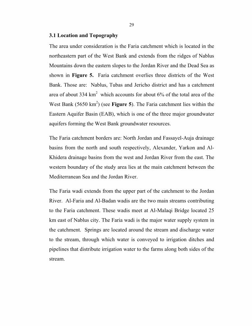
3.1 Location and Topography
The area under consideration is the Faria catchment which is located in the
northeastern part of the West Bank and extends from the ridges of Nablus
Mountains down the eastern slopes to the Jordan River and the Dead Sea as
shown in Figure 5. Faria catchment overlies three districts of the West
Bank. Those are: Nablus, Tubas and Jericho district and has a catchment
area of about 334 km2 which accounts for about 6% of the total area of the
West Bank (5650 km2) (see Figure 5). The Faria catchment lies within the
Eastern Aquifer Basin (EAB), which is one of the three major groundwater
aquifers forming the West Bank groundwater resources.
The Faria catchment borders are: North Jordan and Fassayel-Auja drainage
basins from the north and south respectively, Alexander, Yarkon and Al-
Khidera drainage basins from the west and Jordan River from the east. The
western boundary of the study area lies at the main catchment between the
Mediterranean Sea and the Jordan River.
The Faria wadi extends from the upper part of the catchment to the Jordan
River. Al-Faria and Al-Badan wadis are the two main streams contributing
to the Faria catchment. These wadis meet at Al-Malaqi Bridge located 25
km east of Nablus city. The Faria wadi is the major water supply system in
the catchment. Springs are located around the stream and discharge water
to the stream, through which water is conveyed to irrigation ditches and
pipelines that distribute irrigation water to the farms along both sides of the
stream.
30
West Bank DistrictsSalfitJeninTubasNablusJerichoHebronTulkarmQalqiliyaJerusalemBethlehemRamallah and Al-Bireh
Dead SeaFaria Catchment West Bank Boundary
N
Prepared byEng. Sameer Shadeed
0 40 Kilometers
$TNablus
#
Jordan River
Figure 5: Location of the Faria Catchment within the West Bank
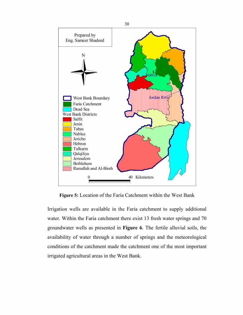
Irrigation wells are available in the Faria catchment to supply additional
water. Within the Faria catchment there exist 13 fresh water springs and 70
groundwater wells as presented in Figure 6. The fertile alluvial soils, the
availability of water through a number of springs and the meteorological
conditions of the catchment made the catchment one of the most important
irrigated agricultural areas in the West Bank.
31
#Y#Y
#Y#Y#Y#Y
#Y#Y
#Y
#Y
#Y#Y#Y#Y#Y#Y
#Y #Y#Y
#Y #Y
#Y
#Y#Y
#Y
#Y#Y#Y#Y
#Y
#Y #Y#Y#Y#Y#Y#Y#Y#Y#Y
#Y
#Y #Y#Y#Y
#Y
#Y#Y#Y#Y
#Y
#Y#Y
#Y#Y
#Y
#Y#Y#Y
#Y#Y
#Y#Y
$Z$Z
$Z$Z$Z$Z$Z$Z
$Z$Z
$Z
$Z$Z
N
Layout preparerEng. Sameer Shadeed
0 3 6 9 Kilometers
#Y Wells$Z Springs
Catchment Boundary
Figure 6: Springs and Wells within the Faria Catchment
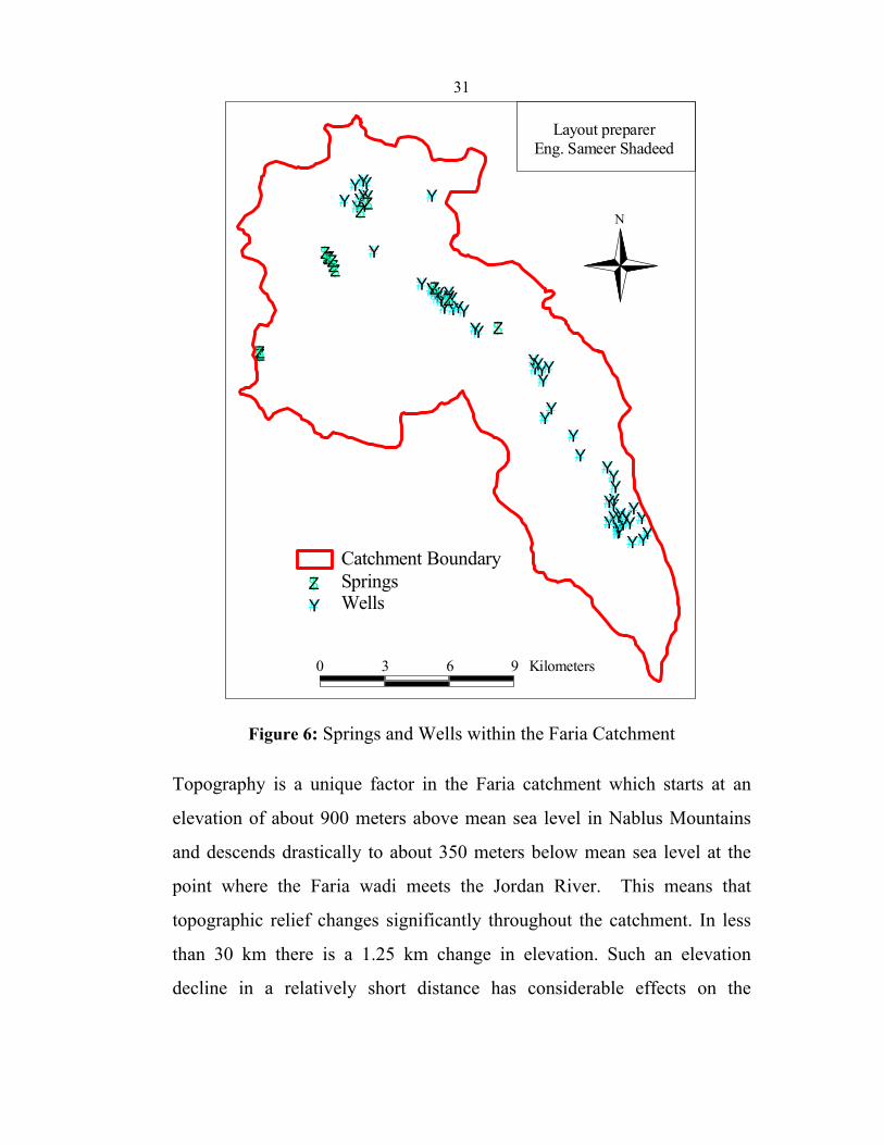
Topography is a unique factor in the Faria catchment which starts at an
elevation of about 900 meters above mean sea level in Nablus Mountains
and descends drastically to about 350 meters below mean sea level at the
point where the Faria wadi meets the Jordan River. This means that
topographic relief changes significantly throughout the catchment. In less
than 30 km there is a 1.25 km change in elevation. Such an elevation
decline in a relatively short distance has considerable effects on the
32
prevailing meteorological conditions in the area as a whole and, in fact,
adds to its importance and uniqueness.
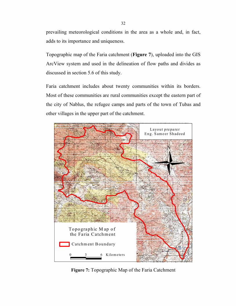
Topographic map of the Faria catchment (Figure 7), uploaded into the GIS
ArcView system and used in the delineation of flow paths and divides as
discussed in section 5.6 of this study.
Faria catchment includes about twenty communities within its borders.
Most of these communities are rural communities except the eastern part of
the city of Nablus, the refugee camps and parts of the town of Tubas and
other villages in the upper part of the catchment.
N
Layou t p re pa re rEng . S am e er Shadeed
Ca tchm ent B oundary
To po graph ic M ap o f the Faria C atch m ent
0 3 6 Kilom ete rs
Figure 7: Topographic Map of the Faria Catchment
33
3.2 Climate
In the West Bank, climatic stations are mainly concentrated in the principal
towns and villages. Since the Faria catchment does not contain significantly
large built up areas, therefore only two climatic stations are located within
the Faria catchment. One of the stations is located in Nablus (570 m
elevation) and the other is located in Al-Jiftlik (-237 m elevation).
Climatic data for these stations were obtained from the Palestine Climate
Data Handbook published by the Meteorological Office of the Ministry of
Transport (MOT) (1998). Climatic data included average monthly values
for maximum and minimum temperature, mean wind speed, mean sunshine
duration, mean relative humidity and pan evaporation. The average values
for the climatic conditions prevailing in the catchment area are presented in
Appendix A1. The information has been spatially delineated using the GIS
ArcView 3.2 software based on data input of temperature and
evapotranspiration.
3.2.1 Wind
The main wind direction is from west, southwest and northwest. Variation
during winter is associated with the pattern of depressions passing from
west to east over the Mediterranean (Ghanem, 1999). The prevailing winds
in the area are the southwest and northwest winds with an annual average
wind speed of 237 km per day in Nablus at a height of 10 meters from
ground surface. When this value is adjusted for 2 meters height (the 2
meters height value is used in most of the potential evapotranspiration
estimates), average wind velocity drops to 185 km per day. During
summer, wind moves with relatively cooler air from the Mediterranean
towards the north, with an average wind speed of 288 km per day in June in
34
Nablus at a height of 10 meters. At night the land areas become cooler,
causing diurnal fluctuations in wind speed, due to the reduction of the
pressure gradient. In winter, the wind moves from west to east over the
Mediterranean, bringing westerly rain bearing winds of average wind speed
209 km per day in January. The Khamaseen, desert storm, may occur
during the period from April to June. During the Khamaseen, the
temperature increases, the humidity decreases and the atmosphere becomes
hazy with dust of desert origin. Wind velocities decrease with elevation,
thus wind velocities in Al-Jiftlik in the lower part of the catchment are
significantly lower than those in Nablus located in the upper part of the
catchment. Existing wind data showed that measurements of wind
velocities were recorded at a height of 10 meters in Nablus and at a height
of 2 meters in Al-Jiftlik. Due to the elevation of Al-Jiftlik which is 237
meters below sea level and the existing mountains surrounding Al-Jiftlik,
wind velocities are much lower than those at Nablus. Annual average wind
velocity in Al-Jiftlik was estimated at 106 km/day at a height of 2 meters
which is much less than the 185 Km/day estimated in Nablus at the same
height from ground surface.
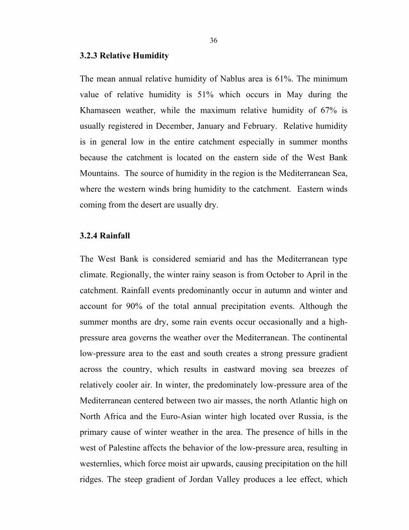
3.2.2 Temperature
Faria catchment is characterized by high temperature variations over space
and over time. Temperatures reduce with increasing elevation in the
catchment. The average temperature variation between Nablus and Al-
Jiftlik is about 5 oC. The mean annual temperature changes from 18 oC in
the western side of the catchment in Nablus to 24 oC in the eastern side of
the catchment at Al-Jiftlik. Figure 8 shows the variation in average
monthly temperatures in Nablus and Al-Faria stations. Spatial
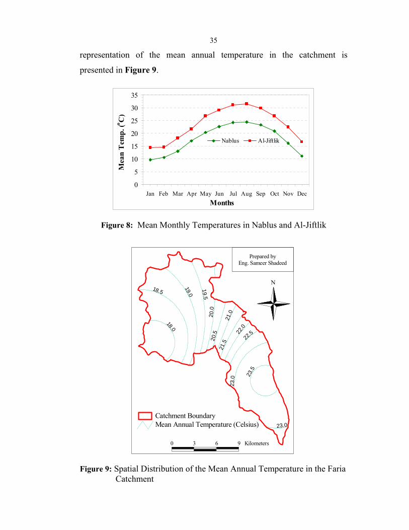
35
representation of the mean annual temperature in the catchment is
presented in Figure 9.
0
5
10
15
20
25
30
35
Jan Feb Mar Apr May Jun Jul Aug Sep Oct Nov DecMonths
Mea
n T
emp.
(o C)
Nablus Al-Jiftlik
Figure 8: Mean Monthly Temperatures in Nablus and Al-Jiftlik 19.0
19.5
18.5
23.0
21.5
20.0
21.0
20.5 22
.0
22.5
18.0
23.5
23.0
N
Prepared byEng. Sameer Shadeed
Mean Annual Temperature (Celsius)Catchment Boundary
0 3 6 9 Kilometers
Figure 9: Spatial Distribution of the Mean Annual Temperature in the Faria Catchment
36
3.2.3 Relative Humidity
The mean annual relative humidity of Nablus area is 61%. The minimum
value of relative humidity is 51% which occurs in May during the
Khamaseen weather, while the maximum relative humidity of 67% is
usually registered in December, January and February. Relative humidity
is in general low in the entire catchment especially in summer months
because the catchment is located on the eastern side of the West Bank
Mountains. The source of humidity in the region is the Mediterranean Sea,
where the western winds bring humidity to the catchment. Eastern winds
coming from the desert are usually dry.
3.2.4 Rainfall
The West Bank is considered semiarid and has the Mediterranean type
climate. Regionally, the winter rainy season is from October to April in the
catchment. Rainfall events predominantly occur in autumn and winter and
account for 90% of the total annual precipitation events. Although the
summer months are dry, some rain events occur occasionally and a high-
pressure area governs the weather over the Mediterranean. The continental
low-pressure area to the east and south creates a strong pressure gradient
across the country, which results in eastward moving sea breezes of
relatively cooler air. In winter, the predominately low-pressure area of the
Mediterranean centered between two air masses, the north Atlantic high on
North Africa and the Euro-Asian winter high located over Russia, is the
primary cause of winter weather in the area. The presence of hills in the
west of Palestine affects the behavior of the low-pressure area, resulting in
westernlies, which force moist air upwards, causing precipitation on the hill
ridges. The steep gradient of Jordan Valley produces a lee effect, which
37
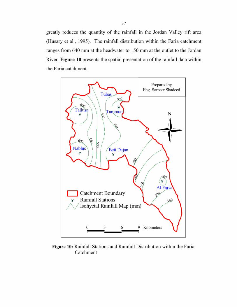
greatly reduces the quantity of the rainfall in the Jordan Valley rift area
(Husary et al., 1995). The rainfall distribution within the Faria catchment
ranges from 640 mm at the headwater to 150 mm at the outlet to the Jordan
River. Figure 10 presents the spatial presentation of the rainfall data within
the Faria catchment.
#Y
#Y
#Y
#Y
#Y
#Y
450500
550
400
300
250
350
200
150
600
200
600
350 Tubas
Nablus
Tammun
Al-Faria
Talluza
Beit Dajan
N
Prepared byEng. Sameer Shadeed
Isohyetal Rainfall Map (mm)#Y Rainfall Stations
Catchment Boundary
0 3 6 9 Kilometers
Figure 10: Rainfall Stations and Rainfall Distribution within the Faria Catchment
38
3.2.5 Evaporation
The Mediterranean climate (hot and dry in the summer, mild and wet in the
winter) has six to seven months of dryness in the year. Winter months
where moisture is available from rain have low evapotranspiration rates.
Summer months with high potential evapotranspiration rates have no rain
and thus actual evapotranspiration is limited by the availability of moisture.
Evaporation rates in Faria regions are measured from a US Class A pan at
Nablus station as shown in the table of Appendix A1. From the table it is
noticed that the average annual evaporation measured at Nablus station is
about 1682 mm. Evapotranspiration is usually smaller than pan evaporation.
Evaporation rates should be multiplied by a pan coefficient (less than 1) to
estimate evapotranspiration rates. A more accurate way to estimate
evapotranspiration is from climatic data.
Monthly potential evapotranspiration rates were estimated according to
Penman-Monteith method as modified by FAO using CROPWAT 4
Windows version 4.2 model (FAO, 1998). The maximum potential rate of
Evapotranspiration was estimated at 1540 mm/year at Al-Jiftlik and 1408
mm/year in Nablus. Although the temperature variability between Nablus
and Al-Jiftlik might indicate a larger difference in evapotranspiration, this
difference was reduced as a result of higher wind velocities in dry summer
months in Nablus.
In the upper part of the Faria catchment, at Nablus, precipitation exceeds
potential evapotranspiration in five months of the year (November through
March). However, in the lower part of the catchment, at Al-Jiftlik,
precipitation exceeds potential evapotranspiration in two months of the
year only (December and January). Therefore, irrigation is required during
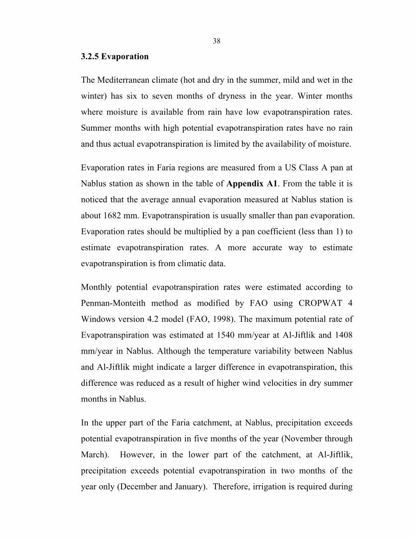
39
most months of the year in the lower part of the catchment in comparison
to the upper part. Figure 11 shows the relation between potential
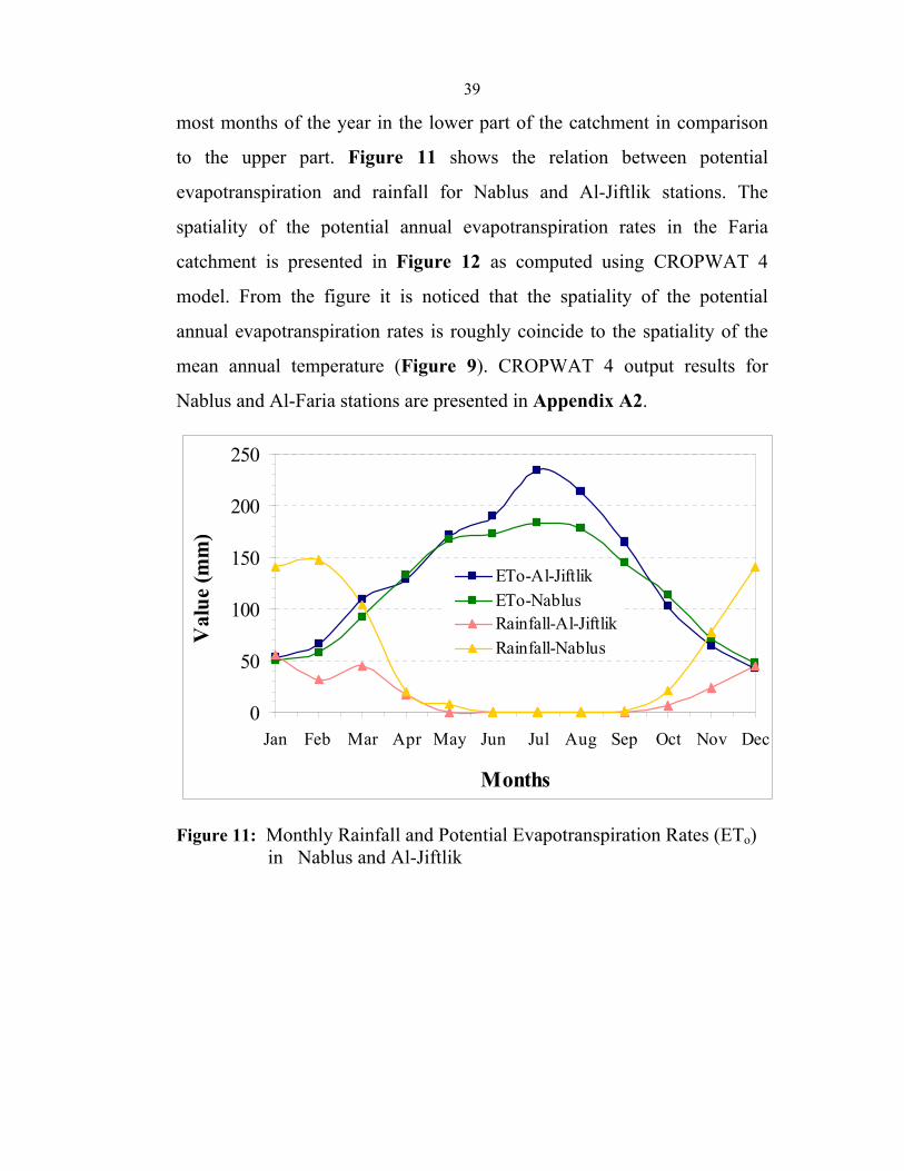
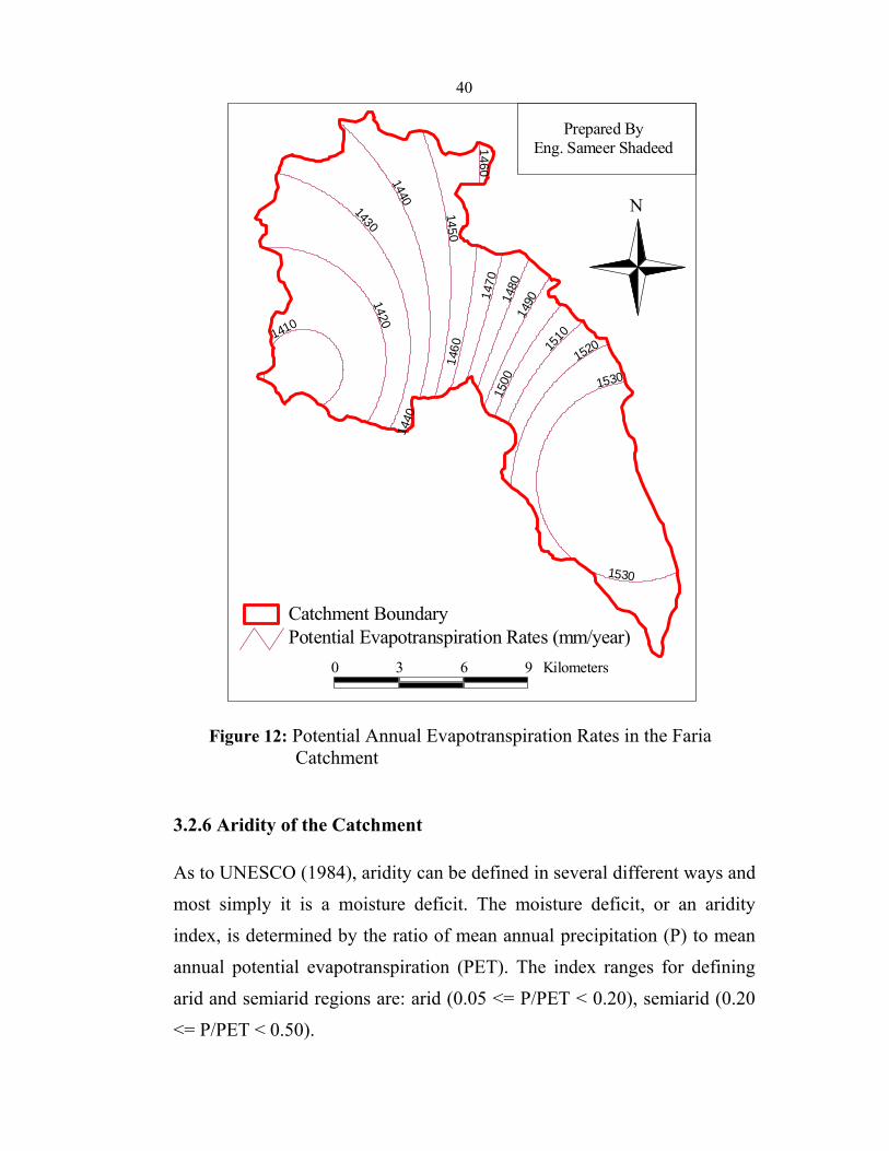
evapotranspiration and rainfall for Nablus and Al-Jiftlik stations. The
spatiality of the potential annual evapotranspiration rates in the Faria
catchment is presented in Figure 12 as computed using CROPWAT 4
model. From the figure it is noticed that the spatiality of the potential
annual evapotranspiration rates is roughly coincide to the spatiality of the
mean annual temperature (Figure 9). CROPWAT 4 output results for
Nablus and Al-Faria stations are presented in Appendix A2.
0
50
100
150
200
250
Jan Feb Mar Apr May Jun Jul Aug Sep Oct Nov Dec
Months
Val
ue (m
m)
ETo-Al-JiftlikETo-NablusRainfall-Al-JiftlikRainfall-Nablus
Figure 11: Monthly Rainfall and Potential Evapotranspiration Rates (ETo) in Nablus and Al-Jiftlik
40
1440
1430
145 0
1420
1530
1520
1490
1460
1480
1470
1500
15101410
1530
146014
40
N
Prepared ByEng. Sameer Shadeed
Potential Evapotranspiration Rates (mm/year)Catchment Boundary
0 3 6 9 Kilometers
Figure 12: Potential Annual Evapotranspiration Rates in the Faria Catchment
3.2.6 Aridity of the Catchment
As to UNESCO (1984), aridity can be defined in several different ways and
most simply it is a moisture deficit. The moisture deficit, or an aridity
index, is determined by the ratio of mean annual precipitation (P) to mean
annual potential evapotranspiration (PET). The index ranges for defining
arid and semiarid regions are: arid (0.05 <= P/PET < 0.20), semiarid (0.20
<= P/PET < 0.50).
41
Monthly potential evapotranspiration rates were estimated according to
Penman-Monteith method as modified by FAO (1998) using CROPWAT 4
Windows version 4.2 model. The results of applying CROPWAT 4 model
are presented in the previous section and Appendix A2. It was estimated
that the annual potential rate of Evapotranspiration is 1540 mm and 1408
mm at Al-Jiftlik and Nablus stations respectively. For these stations, the
long term average annual rainfall is 198 mm and 642 mm respectively.
Therefore, the aridity index is 0.13 for Al-Jiftlik and 0.46 for Nablus. This
means that arid conditions prevail in Al-Jiftlik, whereas semiarid
conditions prevail in Nablus.
3.3 Water Resources
3.3.1 Groundwater Wells
There are 69 wells in the Faria catchment; of which 61 are agricultural
wells, 3 are domestic and 5 are Israeli wells. These wells are drilled in four
sub-aquifers. These sub-aquifers are Eocene, Cenomanian, Neogene and
Pleistocene sub-aquifers. All these wells are located in the study area
mainly in the areas of Ras Al-Faria, Al-Aqrabanieh, Al-Nasaria, Froush
Beit Dajan and Jiftlik along the flexure of wadi Faria.
Based on the available data (Table 1), the total utilization of the Palestinian
wells ranges from 4.4 to 11.5 MCM/year. Data on the pumping rates from
the Israeli wells is available for four wells for only four years from 1997-
2000. The average total abstraction from these four wells was found to be
about 8 MCM/year. Average well abstraction from Israeli wells is about 2
MCM/year. Thus, considering the fifth Israeli well without data available,
the total abstraction from the five Israeli wells in the Faria catchment is
estimated at 10 MCM/year, which is more than the 61 Palestinian
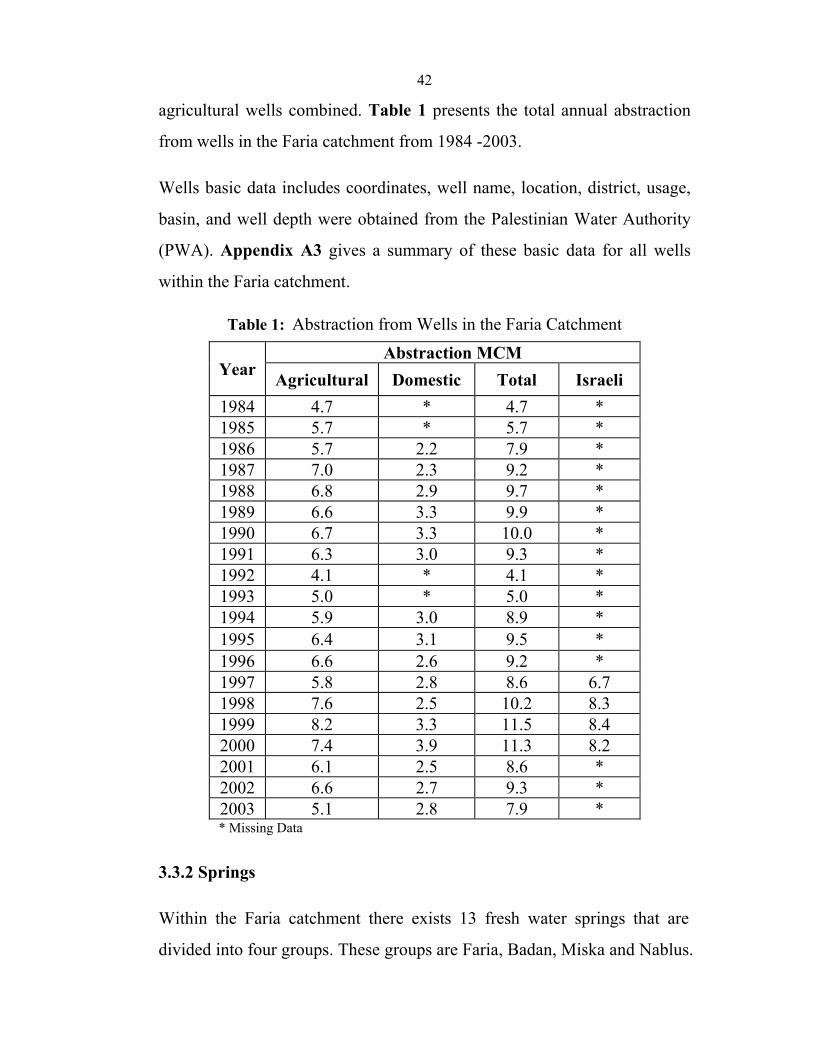
42
agricultural wells combined. Table 1 presents the total annual abstraction
from wells in the Faria catchment from 1984 -2003.
Wells basic data includes coordinates, well name, location, district, usage,
basin, and well depth were obtained from the Palestinian Water Authority
(PWA). Appendix A3 gives a summary of these basic data for all wells
within the Faria catchment.
Table 1: Abstraction from Wells in the Faria Catchment
Year Abstraction MCM
Agricultural Domestic Total Israeli 1984 4.7 * 4.7 * 1985 5.7 * 5.7 * 1986 5.7 2.2 7.9 * 1987 7.0 2.3 9.2 * 1988 6.8 2.9 9.7 * 1989 6.6 3.3 9.9 * 1990 6.7 3.3 10.0 * 1991 6.3 3.0 9.3 * 1992 4.1 * 4.1 * 1993 5.0 * 5.0 * 1994 5.9 3.0 8.9 * 1995 6.4 3.1 9.5 * 1996 6.6 2.6 9.2 * 1997 5.8 2.8 8.6 6.7 1998 7.6 2.5 10.2 8.3 1999 8.2 3.3 11.5 8.4 2000 7.4 3.9 11.3 8.2 2001 6.1 2.5 8.6 * 2002 6.6 2.7 9.3 * 2003 5.1 2.8 7.9 *
* Missing Data
3.3.2 Springs
Within the Faria catchment there exists 13 fresh water springs that are
divided into four groups. These groups are Faria, Badan, Miska and Nablus.

43
The basic data available on these springs include group name, spring name,
coordinates, average annual discharge, minimum annual discharge and
maximum annual discharge. Table 2 presents a summary of these basic
data. Monthly spring discharge measurements for more than 30 years are
available for these springs as presented in Appendix A4. Discharge data of
the springs show high spring discharge variability. Annual discharge from
these springs varies from 3.8 to 38.3 MCM/year with an average amount of
14.4 MCM/year.
The location of the springs and wells within the Faria catchment are shown
in Figure 6.
Table 2: Spring Groups and Spring Information within Faria catchment
Group Spring Name
Coordinates Ave. Annual
DischargeMCM
Min. Annual
Discharge MCM
Max. Annual
DischargeMCM
X (km)
Y (km)
Elevation (m)
Faria El Faria El Duleb
182.40 182.00
188.40 187.95
160 155
5.23 1.27
1.71 0.06
10.53 8.60
Badan Asubian Beida & Hammad Sidreh Tabban Qudeira Jiser
180.52 180.12
179.95 180.42 180.13 180.37
184.56 185.32
185.58 184.82 185.28 185.10
130 215
240 160 215 170
0.19 0.81
1.34 1.38 1.33 0.14
0.14 0.10
0.00 0.98 0.00 0.03
0.23 1.75
8.12 1.63 2.33 0.23
Miska Miska Shibli Abu Saleh
187.03 189.90 186.26
182.90 181.28 183.57
-38 -80 -19
1.32 0.95 0.19
0.02 0.71 0.00
2.21 1.15 0.50
Nablus Balata Dafna
176.20 176.20
179.77 179.90
510 560
0.17 0.13
0.05 0.02
0.55 0.49
Total 14.44 3.81 38.31
3.3.3 Analysis of Springs Discharge
There are sex springs within Al-Badan sub-catchment, in addition to other
two springs that are entirely utilized by the city of Nablus, whereas Al
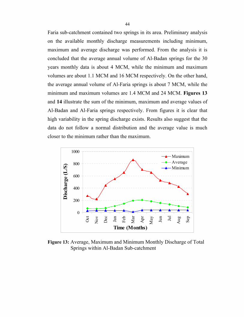
44
Faria sub-catchment contained two springs in its area. Preliminary analysis
on the available monthly discharge measurements including minimum,
maximum and average discharge was performed. From the analysis it is
concluded that the average annual volume of Al-Badan springs for the 30
years monthly data is about 4 MCM, while the minimum and maximum
volumes are about 1.1 MCM and 16 MCM respectively. On the other hand,
the average annual volume of Al-Faria springs is about 7 MCM, while the
minimum and maximum volumes are 1.4 MCM and 24 MCM. Figures 13
and 14 illustrate the sum of the minimum, maximum and average values of
Al-Badan and Al-Faria springs respectively. From figures it is clear that
high variability in the spring discharge exists. Results also suggest that the
data do not follow a normal distribution and the average value is much
closer to the minimum rather than the maximum.
0
200
400
600
800
1000
Oct
Nov Dec Jan
Feb
Mar
Apr
May Jun Jul
Aug Se
p
Time (Months)
Disc
harg
e (L
/S)
MaximumAverageMinimum
Figure 13: Average, Maximum and Minimum Monthly Discharge of Total Springs within Al-Badan Sub-catchment
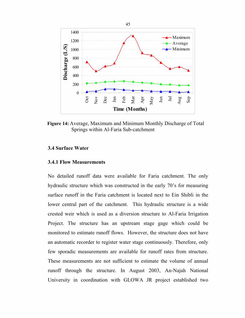
45
0
200
400
600
800
1000
1200
1400
Oct
Nov Dec Jan
Feb
Mar
Apr
May Jun Jul
Aug Se
p
Time (Months)
Disc
harg
e (L
/S)
MaximumAverageMinimum
Figure 14: Average, Maximum and Minimum Monthly Discharge of Total Springs within Al-Faria Sub-catchment
3.4 Surface Water
3.4.1 Flow Measurements
No detailed runoff data were available for Faria catchment. The only
hydraulic structure which was constructed in the early 70’s for measuring
surface runoff in the Faria catchment is located next to Ein Shibli in the
lower central part of the catchment. This hydraulic structure is a wide
crested weir which is used as a diversion structure to Al-Faria Irrigation
Project. The structure has an upstream stage gage which could be
monitored to estimate runoff flows. However, the structure does not have
an automatic recorder to register water stage continuously. Therefore, only
few sporadic measurements are available for runoff rates from structure.
These measurements are not sufficient to estimate the volume of annual
runoff through the structure. In August 2003, An-Najah National
University in coordination with GLOWA JR project established two
46
Venturi Flumes at Jiser Al-Malaqi to measure runoff rates from both Al-
Faria and Al-Badan wadis. GLOWA JR project is an interdisciplinary
project that studies the "Impacts of Global Changes on Water Resources in
Wadis Contributing to the Lower Jordan Basin". GLOWA project is a
German funded project by the German Ministry of Education and Research
and is managed by German, Jordanian and Palestinian institutes. Water
and Environmental Studies Institute (WESI) of An-Najah University is a
counterpartner for Package 2 of GLOWA project researching the water
resources in Jordan River.
The Flume of Al-Badan wadi was designed to measure 25 m3/s and 0.23
m3/s of maximum and minimum flows respectively. Maximum and
minimum flows that can be measured by Al-Faria wadi Flume are 15 m3/s
and 0.19 m3/s respectively. In case of low flows the Parshall Flumes are not
significantly accurate.
There are two reading gauges at each Flume to measure the flow depths at
the critical sections, which are converted into flow rates using the designed
empirical formulas. The constructed Flumes are still working and the
records are available for the two years (2003-2005) since their construction.
The Flumes did not have automatic recorders during the first year. The
automatic recorders were constructed later and are available since the
second year. Photos of the two Flumes are presented in Appendix D1. The
recorded runoff data are tabulated as in Appendix A5.
Surface runoff of the Faria catchment is considered high compared to other
catchments in the West Bank. Within the catchment the runoff decreases
from west to east as the slope becomes relatively gentile eastwards down
the main stream where rainfall rates reduce also.
47
The city of Nablus discharges untreated industrial and domestic wastewater
effluents to Al-Badan wadi while Al-Faria camp discharges untreated
domestic wastewater to Al-Faria wadi. Therefore, the stream flow of the
Faria catchment is a mix of:
1. Runoff generated from winter storms. This includes urban runoff from
the eastern side of the city of Nablus and other built up areas in the
catchment.
2. Untreated wastewater of the eastern part of Nablus and of Al-Faria
camp.
3. Fresh water from springs which provides the baseflow for the wadi
preventing it from drying up during hot summers.
Farmers use part of the flowing water for irrigation while the rest discharge
into the lower Jordan valley or lost through evaporation.
3.4.2 Quality Considerations
No considerable measurements for surface water quality are available for
the Faria streams. All the quality measurements conducted in the area are
performed for the springs and wells. Since the source of water for the Faria
wadi are mostly from springs, then the water quality is dependent on the
water quality of these springs. Measurements for spring water quality
showed that these springs are generally of good water quality especially
chemical quality. The chemical quality data of water from all the springs of
the Faria catchment show low concentrations of salts. Therefore, the
chemical quality of the Faria streams is good and water is suitable for
irrigation (EQA, 2004). A major source of pollution comes from the Nablus
48
municipality. Nablus dumps untreated effluent from its sewage network
directly into the Al-Badan wadi, a tributary of the mean wadi of the Faria
catchment. The Faria refugee camp disposes of some of its solid waste in
pits and the rest by trucking it to a site 1.5 km from the camp to be burned.
The effluent is drained into the wadi a few hundred meters away from the
camp and wastewater from homes is often dumped directly into the streams
or into open ditches.
Another source of water contamination is the livestock that use wadis and
springs as a drinking water source, and pollute the water with fecal matter.
Moreover, local herders bring their sheep and goats to the streams to wash
them and to shear the sheep, thereby polluting the surface waters. Finally,
an extremely significant pollution factor is the waste disposal and use of
agricultural chemicals by the Israeli colonies. However, no information or
data are currently available to be considered in this study.
However, due to the discharge of untreated wastewater into the wadi its
quality has deteriorated significantly. An eye inspection of the wadi and the
wastewater entering into it gives an indication of the high deterioration in
its quality. Historical data and measurements are not available to quantify
such deterioration. Accordingly, samples from the outlet streams (Flumes)
of the upper two sub-catchments were collected and analyzed in the context
of GLOWA JR project. Samples were taken during different times to study
the seasonal variation of the surface water quality. Table 3 shows a
summary of the results for the samples collected during the years 2004 and
2005.
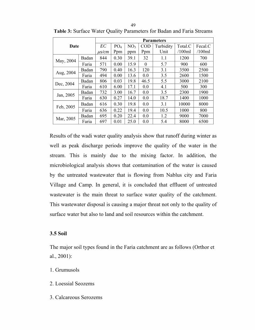
49Table 3: Surface Water Quality Parameters for Badan and Faria Streams
Results of the wadi water quality analysis show that runoff during winter as
well as peak discharge periods improve the quality of the water in the
stream. This is mainly due to the mixing factor. In addition, the
microbiological analysis shows that contamination of the water is caused
by the untreated wastewater that is flowing from Nablus city and Faria
Village and Camp. In general, it is concluded that effluent of untreated
wastewater is the main threat to surface water quality of the catchment.
This wastewater disposal is causing a major threat not only to the quality of
surface water but also to land and soil resources within the catchment.
3.5 Soil
The major soil types found in the Faria catchment are as follows (Orthor et
al., 2001):
1. Grumusols
2. Loessial Seozems
3. Calcareous Serozems
Date Parameters
EC μs/cm
PO4 Ppm
NO3 ppm
CODPpm
TurbidityUnit
Total.C/100ml
Fecal.C/100ml
May, 2004 Badan 844 0.30 39.1 32 1.1 1200 700 Faria 571 0.00 15.9 0 5.7 900 600
Aug, 2004 Badan 790 0.40 16.3 120 3.1 3500 2500 Faria 494 0.00 13.6 0.0 3.5 2600 1500
Dec, 2004 Badan 806 0.03 19.8 46.5 5.5 3000 2100 Faria 610 6.00 17.1 0.0 4.1 500 300
Jan, 2005 Badan 732 3.00 16.7 0.0 3.5 2300 1900 Faria 630 0.27 14.0 0.0 18.7 1400 1000
Feb, 2005 Badan 616 0.30 19.8 0.0 3.1 10000 8000 Faria 636 0.22 19.4 0.0 10.5 1000 800
Mar, 2005 Badan 695 0.20 22.4 0.0 1.2 9000 7000 Faria 697 0.01 25.0 0.0 5.4 8000 6500
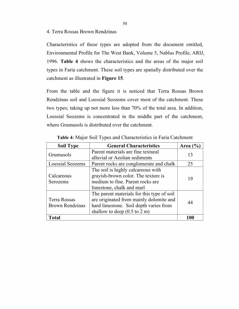
50
4. Terra Rossas Brown Rendzinas
Characteristics of these types are adopted from the document entitled,
Environmental Profile for The West Bank, Volume 5, Nablus Profile, ARIJ,
1996. Table 4 shows the characteristics and the areas of the major soil
types in Faria catchment. These soil types are spatially distributed over the
catchment as illustrated in Figure 15.
From the table and the figure it is noticed that Terra Rossas Brown
Rendzinas soil and Loessial Seozems cover most of the catchment. These
two types; taking up not more less than 70% of the total area. In addition,
Loessial Seozems is concentrated in the middle part of the catchment,
where Grumusols is distributed over the catchment.
Table 4: Major Soil Types and Characteristics in Faria Catchment Soil Type General Characteristics Area (%)
Grumusols Parent materials are fine textural alluvial or Aeolian sediments 13
Loessial Seozems Parent rocks are conglomerate and chalk 25
Calcareous Serozems
The soil is highly calcareous with grayish-brown color. The texture is medium to fine. Parent rocks are limestone, chalk and marl
19
Terra Rossas Brown Rendzinas
The parent materials for this type of soil are originated from mainly dolomite and hard limestone. Soil depth varies from shallow to deep (0.5 to 2 m)
44
Total 100

51
N
Layout preparerEng. Sameer Shadeed
Soil MapGrumusolsLoessial SeozemsCalcareous SerozemsTerra Rossas Brown Rendzinas
Catchment Boundary
0 3 6 9 Kilometers
Figure 15: Soil Types of the Faria Catchment
3.6 Geology
Faria catchment is a structurally complex system with Al-Faria Anticline
that trends northeast to southwest acting as the primary controlling feature.
Additionally, a series of smaller faults and joints perpendicular to this
anticline have a significant effect on the surface water drainage area. The
geological structure of the Faria catchment is composed form limestone,
dolomite and marl. The rocks vary in its thickness, some of them are more
than two meters and some of them are intermediate thickness of about 40-
100cm. The rock formations were deposited at the second time Mezosy and
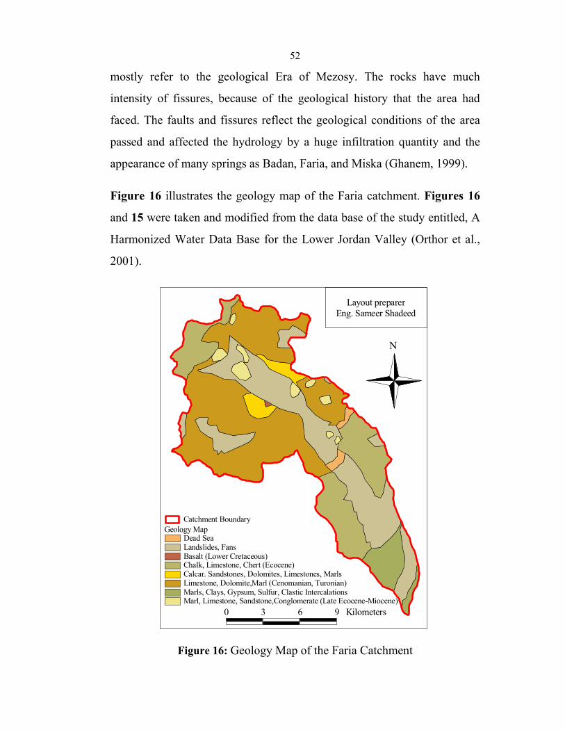
52
mostly refer to the geological Era of Mezosy. The rocks have much
intensity of fissures, because of the geological history that the area had
faced. The faults and fissures reflect the geological conditions of the area
passed and affected the hydrology by a huge infiltration quantity and the
appearance of many springs as Badan, Faria, and Miska (Ghanem, 1999).
Figure 16 illustrates the geology map of the Faria catchment. Figures 16
and 15 were taken and modified from the data base of the study entitled, A
Harmonized Water Data Base for the Lower Jordan Valley (Orthor et al.,
2001).
N
Layout preparerEng. Sameer Shadeed
Geology MapDead SeaLandslides, FansBasalt (Lower Cretaceous)Chalk, Limestone, Chert (Ecocene)Calcar. Sandstones, Dolomites, Limestones, MarlsLimestone, Dolomite,Marl (Cenomanian, Turonian)Marls, Clays, Gypsum, Sulfur, Clastic IntercalationsMarl, Limestone, Sandstone,Conglomerate (Late Ecocene-Miocene)
Catchment Boundary
0 3 6 9 Kilometers
Figure 16: Geology Map of the Faria Catchment
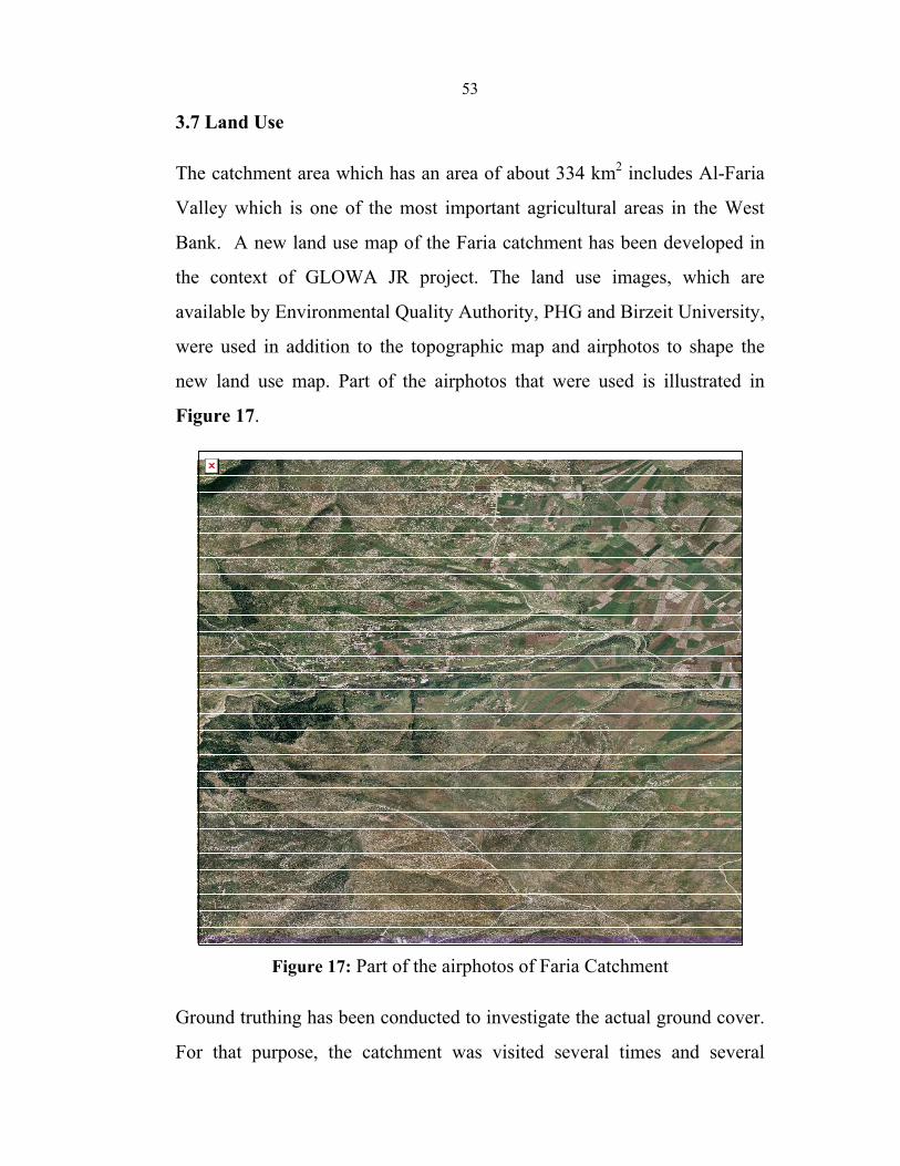
53
3.7 Land Use
The catchment area which has an area of about 334 km2 includes Al-Faria
Valley which is one of the most important agricultural areas in the West
Bank. A new land use map of the Faria catchment has been developed in
the context of GLOWA JR project. The land use images, which are
available by Environmental Quality Authority, PHG and Birzeit University,
were used in addition to the topographic map and airphotos to shape the
new land use map. Part of the airphotos that were used is illustrated in
Figure 17.
Figure 17: Part of the airphotos of Faria Catchment
Ground truthing has been conducted to investigate the actual ground cover.
For that purpose, the catchment was visited several times and several
54
photos were snapped that cover the natures of the catchment as presented in
Appendix D2.
The land use map of the Faria catchment was classified into four classes.
These classes are artificial surfaces, agricultural areas, forests and semi
natural areas and water bodies. Table 5 presents these classes, the area of
each class, its categories and its percent from the whole catchment. The
following is a description of these land use classes.
1. Artificial Surfaces
The artificial surfaces in the catchment are composed of refugee camps,
urban fabrics, Israeli colonies and military camps. The military camps and
colonies are used by the Israeli occupation authorities and settlers. The total
area of the artificial surfaces is 18047 dunum presenting about 5.5 % of the
total area of the catchment. The actual figure is higher due to the fact that
most of the roads and associated land were kept out of the scope of the
study because of the unit limitations. This percentage is less than that of
artificial surfaces in the West Bank (8%) which indicates that the area is
not densely populated due to the harsh topography of the nonagricultural
area in addition to the political restrictions (EQA, 2004).
2. Agricultural Areas
The agricultural land in the catchment is composed of an arable land and
heterogeneous agricultural areas. Arable land involves non-irrigated arable
land, drip-irrigated arable land, olive groves, palm groves and citrus
plantations. The heterogeneous agricultural areas involve irrigated and non-
irrigated complex cultivated pattern and land principally occupied by
55
agriculture with significant areas of natural vegetation. The area of the
agricultural part of Faria catchment is 115447 dunum which represents
about 34.4%. This percentage is lower than that of the West Bank of about
39% (EQA, 2004).
3. Forests and Semi Natural Bodies
This group of land use cover is composed of coniferous forests, natural
grassland, bare rocks, sparsely vegetated area and halophytes. The forests
and semi natural bodies in the Faria catchment occupy an area of about
201087 dunum representing 60% from the total area. It is worth mentioning
that most of the Israeli colonies were built at the expense of forests and
semi natural areas under the cover of many military laws that consider the
forests and vast natural areas as state owned land.
4. Water Bodies
No perennial rivers are available in West Bank other than the Jordan River
that represents the eastern border of West Bank and Faria wadi. Most of the
water courses are seasonal and could be added to the land use maps as
linear features of a width less than the threshold of the smallest unit
mapped.
There are no water bodies controlled by the Palestinians that are large
enough to be drawn on the maps of this study. On the other hand there are
few water bodies on the Jordan Valley and Faria stream near the Jordan
River that are controlled by the Israeli occupation and are utilized for
irrigation and fishing (EQA, 2004). One of the artificial water surfaces
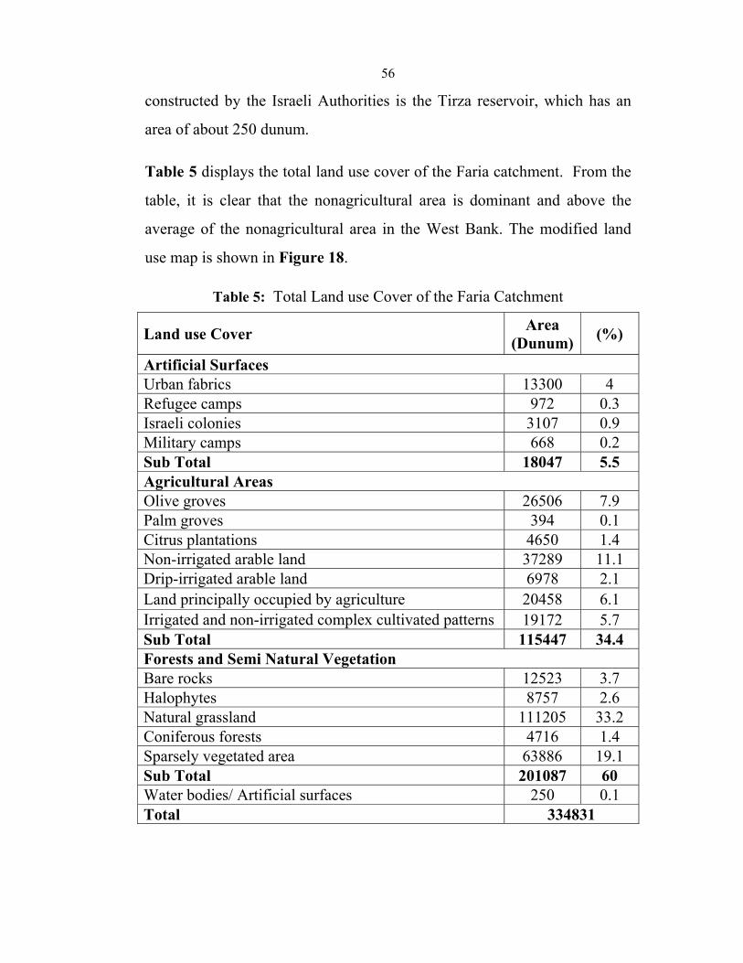
56
constructed by the Israeli Authorities is the Tirza reservoir, which has an
area of about 250 dunum.
Table 5 displays the total land use cover of the Faria catchment. From the
table, it is clear that the nonagricultural area is dominant and above the
average of the nonagricultural area in the West Bank. The modified land
use map is shown in Figure 18.
Table 5: Total Land use Cover of the Faria Catchment
Land use Cover Area (Dunum) (%)
Artificial Surfaces Urban fabrics 13300 4 Refugee camps 972 0.3 Israeli colonies 3107 0.9 Military camps 668 0.2 Sub Total 18047 5.5 Agricultural Areas Olive groves 26506 7.9 Palm groves 394 0.1 Citrus plantations 4650 1.4 Non-irrigated arable land 37289 11.1 Drip-irrigated arable land 6978 2.1 Land principally occupied by agriculture 20458 6.1 Irrigated and non-irrigated complex cultivated patterns 19172 5.7 Sub Total 115447 34.4 Forests and Semi Natural Vegetation Bare rocks 12523 3.7 Halophytes 8757 2.6 Natural grassland 111205 33.2 Coniferous forests 4716 1.4 Sparsely vegetated area 63886 19.1 Sub Total 201087 60 Water bodies/ Artificial surfaces 250 0.1 Total 334831
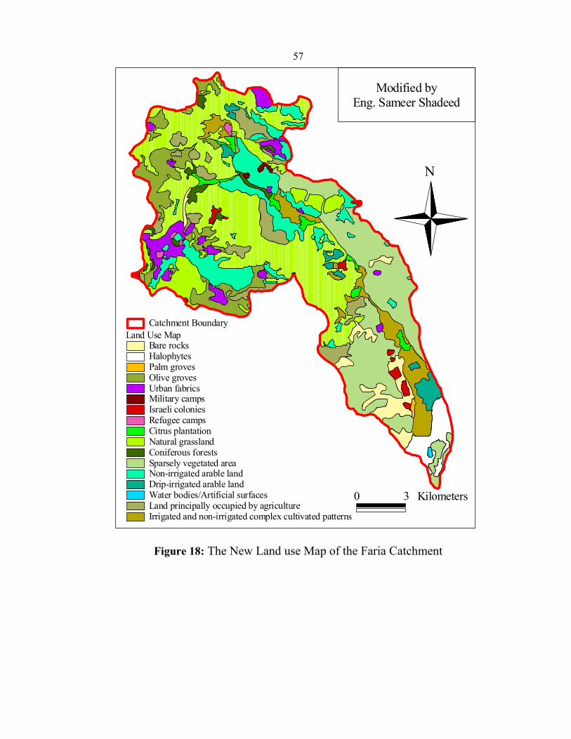
57
N
Modified byEng. Sameer Shadeed
Land Use MapBare rocksHalophytesPalm grovesOlive grovesUrban fabricsMilitary campsIsraeli coloniesRefugee campsCitrus plantationNatural grasslandConiferous forestsSparsely vegetated areaNon-irrigated arable landDrip-irrigated arable landWater bodies/Artificial surfacesLand principally occupied by agricultureIrrigated and non-irrigated complex cultivated patterns
Catchment Boundary
0 3 Kilometers
Figure 18: The New Land use Map of the Faria Catchment

58
CHAPTER FOUR
RAINFALL ANALYSIS
59
4.1 Rainfall Stations
The Faria catchment is gauged by six rainfall stations that record rainfall.
These stations are: Nablus, Taluza, Tammon, Tubas, Beit Dajan and Al-
Faria stations. Before 1994, these stations were controlled by the Israeli
Authorities. After the establishment of the Palestinian Authority, the
stations except one became under the control of the Palestinians. The
Nablus station is a regular weather station in which most climatic data are
measured. Monthly and annual precipitation for this station is available for
more than 55 years.
Al-Faria station is located in Al-Jiftlik village in the lower part of the
catchment and is still under Israeli control. This station was established by
the Jordanian government as an agricultural experimental station similar to
the Deir Alla station on the eastern side of the Jordan River. The station
was taken over by the Israeli Occupation Authorities in 1967. The Israeli
Authorities neglected the station and therefore its role in serving the
Palestinian farmers became insignificant. In 1994, when the Palestinian
Authority was established, the Israeli Authorities refused to hand it over to
the Palestinians. Therefore, data available from this station is limited to
only few years.
The other four rainfall stations are located in the schools of Taluza, Tubas,
Tammon and Beit Dajan (see Figure 10). These stations are simple rain
gages which measure daily precipitation. Data from these stations cover
also monthly and annual precipitation for 30 to 40 years. No rainfall
intensity charts are available in the catchment except from Nablus station
where few years are covered and are available. This is due to lack of
continuous measuring instruments for precipitation or other weather data.
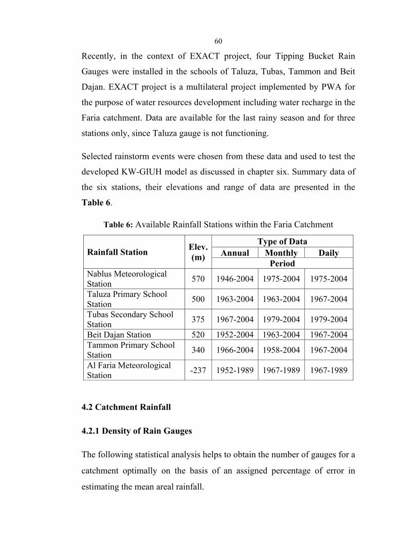
60
Recently, in the context of EXACT project, four Tipping Bucket Rain
Gauges were installed in the schools of Taluza, Tubas, Tammon and Beit
Dajan. EXACT project is a multilateral project implemented by PWA for
the purpose of water resources development including water recharge in the
Faria catchment. Data are available for the last rainy season and for three
stations only, since Taluza gauge is not functioning.
Selected rainstorm events were chosen from these data and used to test the
developed KW-GIUH model as discussed in chapter six. Summary data of
the six stations, their elevations and range of data are presented in the
Table 6.
Table 6: Available Rainfall Stations within the Faria Catchment
4.2 Catchment Rainfall
4.2.1 Density of Rain Gauges
The following statistical analysis helps to obtain the number of gauges for a
catchment optimally on the basis of an assigned percentage of error in
estimating the mean areal rainfall.
Rainfall Station Elev.(m)
Type of Data Annual Monthly Daily
Period Nablus Meteorological Station 570 1946-2004 1975-2004 1975-2004
Taluza Primary School Station 500 1963-2004 1963-2004 1967-2004
Tubas Secondary School Station 375 1967-2004 1979-2004 1979-2004
Beit Dajan Station 520 1952-2004 1963-2004 1967-2004 Tammon Primary School Station 340 1966-2004 1958-2004 1967-2004
Al Faria Meteorological Station -237 1952-1989 1967-1989 1967-1989
612
⎪⎭
⎪⎬⎫
⎪⎩
⎪⎨⎧
=p
v
ECN 1
Where N is the optimal number of stations, Ep the allowable percentage of
error in the estimation of mean aerial rainfall, Cv is the coefficient of
variation of the rainfall from the existing stations in percentage. Coefficient
of variation can be calculated applying the following steps on the data of
existing n stations.
1. Calculate the mean of rainfall from the equation ( )∑= iav PnP 1 2
2. Calculate the standard deviation as ( )
( ) 2
1
21 1
1
⎭⎬⎫
⎩⎨⎧
−−
= ∑− avin PPn
σ 3
3. Compute the coefficient of variation as av
nv P
C 1001 ×= −σ 4
If the allowable percent of error in estimating the mean rainfall is taken
higher, then the catchment will require fewer numbers of gauges and vice-
versa. The allowable percentage of error Ep is normally taken as 10%.
While computing the value of Cv and if its value comes less than 10%, it
can be assumed that the existing stations are sufficient for the catchment.
The additional station required for the catchment can be found as (N-n).
Annual rainfall values are normally used in the above analysis. Additional
stations are to be established at the appropriate locations giving an even
distribution over the catchment (Patra, 2001).
Based on information from the six stations in Faria catchment, the above
statistical parameters have been calculated:
avP = 431.4
1−nσ = 175.1
62
vC = 40.6
N = 11
Based on a 12% permissible error and rainfall data of available stations, the
minimum required number of stations is 11.
Existing stations (n) = 6
Additional stations required = (N-n) = 5
4.2.2 Consistency of Rainfall Data
When analyzing rainfall data; it is essential to check the consistency of the
records of the rainfall stations. For Faria catchment, the missing data were
first estimated, and then consistency analysis was applied.
Double mass curve technique was used to check the consistency of the
stations of the Faria catchment. The cumulative rainfall data of a specific
station is plotted against the accumulative average rainfall of the remaining
stations. The results of the consistency analysis are plotted in Figure 19.
From the figure, it is clear that all the stations are internally consistent, and
the data can be further analyzed. The data plotted in Figure 19 are for the
periods 1946-2003 for all the stations except for Al-Faria station, which are
for 1951-1989.
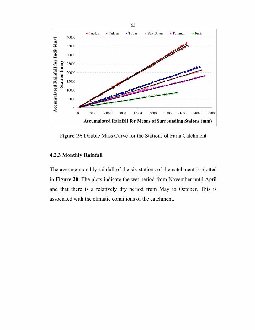
63
0
5000
10000
15000
20000
25000
30000
35000
40000
0 3000 6000 9000 12000 15000 18000 21000 24000 27000
Accumulated Rainfall for Means of Surrounding Staions (mm)
Acc
umul
ated
Rai
nfal
l for
Indi
vidu
al
Stat
ion
(mm
)
Nablus Taluza Tubas Beit Dajan Tammon Faria
Figure 19: Double Mass Curve for the Stations of Faria Catchment
4.2.3 Monthly Rainfall
The average monthly rainfall of the six stations of the catchment is plotted
in Figure 20. The plots indicate the wet period from November until April
and that there is a relatively dry period from May to October. This is
associated with the climatic conditions of the catchment.
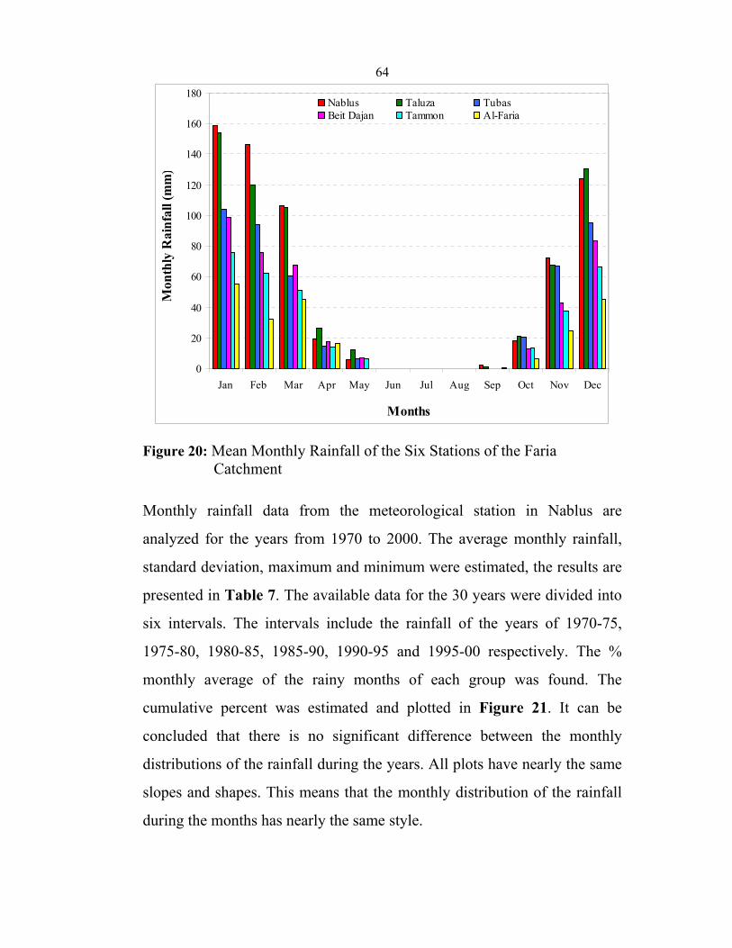
64
0
20
40
60
80
100
120
140
160
180
Jan Feb Mar Apr May Jun Jul Aug Sep Oct Nov Dec
Months
Mon
thly
Rai
nfal
l (m
m)
Nablus Taluza TubasBeit Dajan Tammon Al-Faria
Figure 20: Mean Monthly Rainfall of the Six Stations of the Faria Catchment
Monthly rainfall data from the meteorological station in Nablus are
analyzed for the years from 1970 to 2000. The average monthly rainfall,
standard deviation, maximum and minimum were estimated, the results are
presented in Table 7. The available data for the 30 years were divided into
six intervals. The intervals include the rainfall of the years of 1970-75,
1975-80, 1980-85, 1985-90, 1990-95 and 1995-00 respectively. The %
monthly average of the rainy months of each group was found. The
cumulative percent was estimated and plotted in Figure 21. It can be
concluded that there is no significant difference between the monthly
distributions of the rainfall during the years. All plots have nearly the same
slopes and shapes. This means that the monthly distribution of the rainfall
during the months has nearly the same style.

65Table 7: Monthly Rainfall Totals of Nablus Station (mm)
Year Sept. Oct. Nov. Dec. Jan. Feb. Mar. Apr. May.70-71 8.5 7.1 9.5 124.6 104.6 110.9 49.3 224.6 0.0 71-72 0.0 0.0 57.3 184.3 140.7 167.2 94.3 27.3 0.0 72-73 0.1 14.0 39.6 63.6 163.9 23.2 104.3 12.5 21.8 73-74 0.0 16.3 105.5 66.5 389.3 115.6 41.3 39.5 0.0 74-75 0.0 0.0 55.4 137.1 55.4 194.6 82.0 4.2 0.0 75-76 23.1 3.8 47.2 108.3 93.1 152.0 150.1 27.0 0.0 76-77 0.2 32.7 90.1 46.6 158.5 73.1 128.2 85.7 1.5 77-78 0.0 82.6 2.9 192.6 79.2 60.0 82.8 8.2 0.078-79 0.0 20.1 6.7 104.2 116.7 20.4 75.7 5.0 0.3 79-80 0.0 39.7 158.9 226.5 113.8 165.4 155.5 21.8 1.7 80-81 0.4 15.0 8.9 192.7 211.3 142.5 67.3 23.1 0.081-82 0.0 0.0 135.1 19.9 92.6 171.2 129.6 7.0 2.3 82-83 0.0 10.3 0.0 115.8 267.0 322.9 219.9 14.8 3.6 83-84 0.9 0.0 70.4 24.2 155.2 85.2 0.0 0.0 0.0 84-85 0.0 21.5 29.6 58.5 65.5 245.3 20.1 23.2 1.4 85-86 0.0 19.9 47.1 42.9 93.0 163.2 48.7 46.8 65.1 86-87 0.5 52.4 249.6 141.4 130.0 62.3 120.0 1.9 0.0 87-88 0.0 52.9 23.2 224.0 126.9 310.9 94.9 0.0 0.0 88-89 0.0 16.0 55.8 236.7 96.3 46.6 115.2 0.0 0.089-90 0.0 5.9 94.9 128.3 131.6 98.9 53.3 53.0 0.0 90-91 0.0 3.5 24.3 9.5 251.4 74.3 103.8 30.1 8.0 91-92 0.0 12.7 153.5 472.2 266.8 444.7 69.7 4.7 28.5 92-93 0.0 0.0 84.9 360.9 142.3 117.7 68.5 5.8 18.5 93-94 0.0 14.7 20.8 28.7 192.5 114.0 129.1 9.0 0.0 94-95 0.0 20.6 263.5 186.0 57.9 95.4 43.1 35.3 0.2 95-96 0.0 1.8 118.8 59.2 229.8 35.9 228.7 33.4 0.0 96-97 0.0 34.1 16.4 85.44 166.0 268.6 233.1 22.7 40.297-98 17.6 16.3 59.9 167.9 148.2 91.9 244.5 5.0 7.8 98-99 1.6 1.6 4.9 40.3 169.1 64.4 41.5 21.6 0.0 99-00 0.0 5.8 16.3 39.9 471.2 84.7 80.1 0.4 0.0
AVG 1.8 17.5 68.4 129.6 162.7 137.4 102.5 26.5 6.7 STD 5.3 19.5 68.3 104.4 93.6 97.9 63.4 42.0 14.7 MAX 23.1 82.6 263.5 472.2 471.2 444.7 244.5 224.6 65.1 MIN 0.0 0.0 0.0 9.5 55.4 20.4 0.0 0.0 0.0
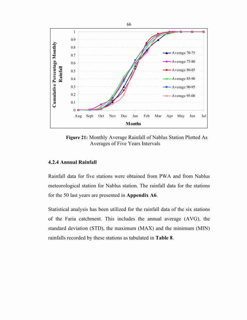
66
0
0.1
0.2
0.3
0.4
0.5
0.6
0.7
0.8
0.9
1
Aug Sept Oct Nov Dec Jan Feb Mar Apr May Jun Jul
Months
Cum
ulat
ive
Perc
enta
ge M
onth
ly
Rai
nfal
l
Average 70-75
Average 75-80
Average 80-85
Average 85-90
Average 90-95
Average 95-00
Figure 21: Monthly Average Rainfall of Nablus Station Plotted As Averages of Five Years Intervals
4.2.4 Annual Rainfall
Rainfall data for five stations were obtained from PWA and from Nablus
meteorological station for Nablus station. The rainfall data for the stations
for the 50 last years are presented in Appendix A6.
Statistical analysis has been utilized for the rainfall data of the six stations
of the Faria catchment. This includes the annual average (AVG), the
standard deviation (STD), the maximum (MAX) and the minimum (MIN)
rainfalls recorded by these stations as tabulated in Table 8.
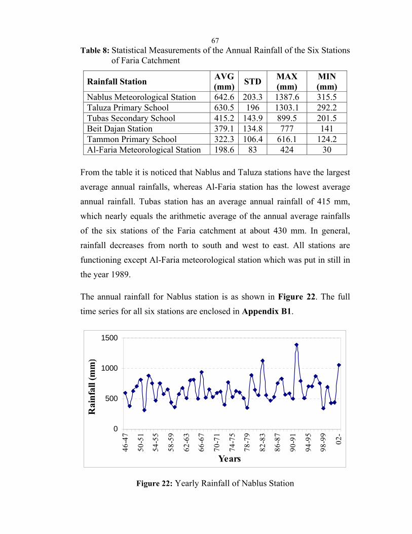
67Table 8: Statistical Measurements of the Annual Rainfall of the Six Stations
of Faria Catchment
From the table it is noticed that Nablus and Taluza stations have the largest
average annual rainfalls, whereas Al-Faria station has the lowest average
annual rainfall. Tubas station has an average annual rainfall of 415 mm,
which nearly equals the arithmetic average of the annual average rainfalls
of the six stations of the Faria catchment at about 430 mm. In general,
rainfall decreases from north to south and west to east. All stations are
functioning except Al-Faria meteorological station which was put in still in
the year 1989.
The annual rainfall for Nablus station is as shown in Figure 22. The full
time series for all six stations are enclosed in Appendix B1.
0
500
1000
1500
46-4
7
50-5
1
54-5
5
58-5
9
62-6
3
66-6
7
70-7
1
74-7
5
78-7
9
82-8
3
86-8
7
90-9
1
94-9
5
98-9
9
02-
Years
Rai
nfal
l (m
m)
Figure 22: Yearly Rainfall of Nablus Station
Rainfall Station AVG(mm) STD MAX
(mm) MIN (mm)
Nablus Meteorological Station 642.6 203.3 1387.6 315.5 Taluza Primary School 630.5 196 1303.1 292.2 Tubas Secondary School 415.2 143.9 899.5 201.5 Beit Dajan Station 379.1 134.8 777 141 Tammon Primary School 322.3 106.4 616.1 124.2 Al-Faria Meteorological Station 198.6 83 424 30
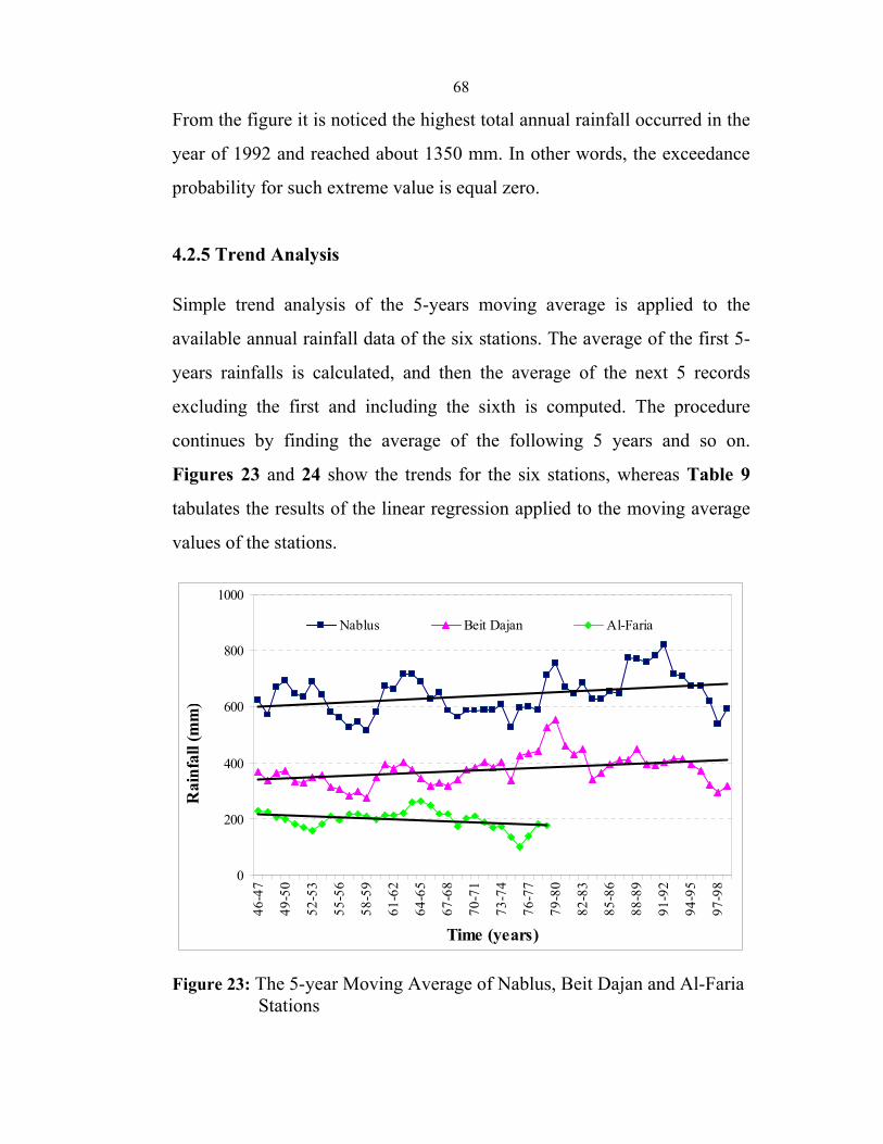
68
From the figure it is noticed the highest total annual rainfall occurred in the
year of 1992 and reached about 1350 mm. In other words, the exceedance
probability for such extreme value is equal zero.
4.2.5 Trend Analysis
Simple trend analysis of the 5-years moving average is applied to the
available annual rainfall data of the six stations. The average of the first 5-
years rainfalls is calculated, and then the average of the next 5 records
excluding the first and including the sixth is computed. The procedure
continues by finding the average of the following 5 years and so on.
Figures 23 and 24 show the trends for the six stations, whereas Table 9
tabulates the results of the linear regression applied to the moving average
values of the stations.
0
200
400
600
800
1000
46-4
7
49-5
0
52-5
3
55-5
6
58-5
9
61-6
2
64-6
5
67-6
8
70-7
1
73-7
4
76-7
7
79-8
0
82-8
3
85-8
6
88-8
9
91-9
2
94-9
5
97-9
8
Time (years)
Rai
nfal
l (m
m)
Nablus Beit Dajan Al-Faria
Figure 23: The 5-year Moving Average of Nablus, Beit Dajan and Al-Faria Stations
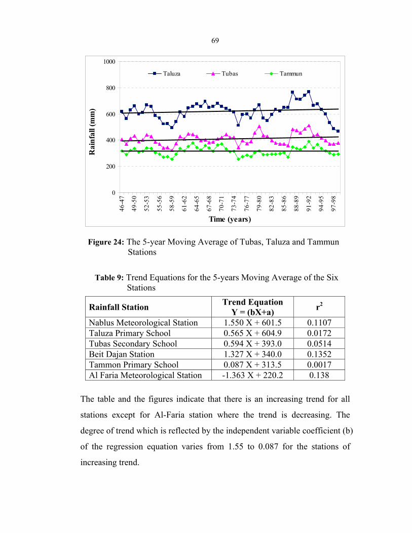
69
0
200
400
600
800
1000
46-4
7
49-5
0
52-5
3
55-5
6
58-5
9
61-6
2
64-6
5
67-6
8
70-7
1
73-7
4
76-7
7
79-8
0
82-8
3
85-8
6
88-8
9
91-9
2
94-9
5
97-9
8
Time (years)
Rai
nfal
l (m
m)
Taluza Tubas Tammun
Figure 24: The 5-year Moving Average of Tubas, Taluza and Tammun Stations
Table 9: Trend Equations for the 5-years Moving Average of the Six Stations
Rainfall Station Trend Equation Y = (bX+a) r2
Nablus Meteorological Station 1.550 X + 601.5 0.1107 Taluza Primary School 0.565 X + 604.9 0.0172 Tubas Secondary School 0.594 X + 393.0 0.0514 Beit Dajan Station 1.327 X + 340.0 0.1352 Tammon Primary School 0.087 X + 313.5 0.0017 Al Faria Meteorological Station -1.363 X + 220.2 0.138
The table and the figures indicate that there is an increasing trend for all
stations except for Al-Faria station where the trend is decreasing. The
degree of trend which is reflected by the independent variable coefficient (b)
of the regression equation varies from 1.55 to 0.087 for the stations of
increasing trend.
70
The significance of the regression equations of the trends can be evaluated
by testing the hypothesis Ho: b=0. If this hypothesis is accepted, then
estimated Y equals mean Y, i.e.: ^Y Y
−
= , where ^Y is estimated Y and Y
−
is
mean Y, or the regression line does not explain a significant amount of the
variation in Y, where Y = bX + a.
In this situation one would use mean Y as an estimator for Y regardless of
the value of X. The hypothesis Ho: b=Bo=0 is equivalent to the hypothesis
Ho: r = 0, where r is the correlation coefficient. Test of hypothesis
concerning (b) can be done noting that
o
b
b Bs
⎛ ⎞−⎜ ⎟⎝ ⎠
5
has t-distribution with (n-2) degrees of freedom. Thus the hypothesis Ho:
b=Bo=0 versus Ho: b≠Bo is tested by computing
o
b
b Bts
⎛ ⎞−= ⎜ ⎟⎝ ⎠
6
Ho is rejected if
t > 1 , 2
2n
t α− −
The t-test has been conducted for 90% and 95% confidence intervals. The
above testing procedure is described in (Hann ,1977). The results of testing
are presented in Table 10. From the table it is noticed that the hypothesis
Ho: Bo=0 versus Ho: Bo≠0 is accepted for all stations except for Nablus and
Beit Dajan stations where the hypothesis is rejected. This means that there
is no significant trend of the 5-years moving average rainfall within the
Faria catchment except for Nablus and Beit Dajan stations.
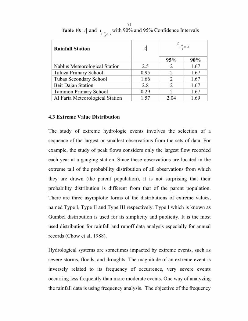
71 Table 10: t and
1 , 22
nt α− −
with 90% and 95% Confidence Intervals
Rainfall Station t 1 , 22
nt α− −
95% 90% Nablus Meteorological Station 2.5 2 1.67 Taluza Primary School 0.95 2 1.67Tubas Secondary School 1.66 2 1.67 Beit Dajan Station 2.8 2 1.67 Tammon Primary School 0.29 2 1.67 Al Faria Meteorological Station 1.57 2.04 1.69
4.3 Extreme Value Distribution
The study of extreme hydrologic events involves the selection of a
sequence of the largest or smallest observations from the sets of data. For
example, the study of peak flows considers only the largest flow recorded
each year at a gauging station. Since these observations are located in the
extreme tail of the probability distribution of all observations from which
they are drawn (the parent population), it is not surprising that their
probability distribution is different from that of the parent population.
There are three asymptotic forms of the distributions of extreme values,
named Type I, Type II and Type III respectively. Type I which is known as
Gumbel distribution is used for its simplicity and publicity. It is the most
used distribution for rainfall and runoff data analysis especially for annual
records (Chow et al, 1988).
Hydrological systems are sometimes impacted by extreme events, such as
severe storms, floods, and droughts. The magnitude of an extreme event is
inversely related to its frequency of occurrence, very severe events
occurring less frequently than more moderate events. One way of analyzing
the rainfall data is using frequency analysis. The objective of the frequency

72
analysis of hydrologic data is to relate the magnitude of extreme events to
their frequency of occurrence through the use of probability distribution
(Chow et al., 1988).
4.3.1 Gumbel Distribution
For the purpose of extreme value analysis, the following procedure has
been followed:
1. The annual rainfall values were arranged in descending order over the
recorded period and each value was given a rank, r.
2. For each value of rainfall, denoted by x, the probability of exceedance,
P(x) was calculated using the Gringorten formula which is appropriate for
the analysis of extremes (Chow et al., 1988):
)12.0()44.0()(
+−
=nrxP 7
where:
x: annual rainfall
P(x): the probability of exceedance
r: the rank of x
n: the total number of recorded years
3. The probability of non-exceedance was calculated using the following
relation:
)12.0()44.0(
1)(1)(+−
−=−=nr
xPxF 8
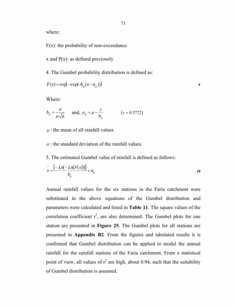
73
where:
F(x): the probability of non-exceedance
x and P(x): as defined previously
4. The Gumbel probability distribution is defined as:
( )))(exp(exp)( gg axbxF −−−= 9
Where:
6σπ
=gb and, g
g ba γμ −= ( )5772.0=γ
μ : the mean of all rainfall values
σ : the standard deviation of the rainfall values
5. The estimated Gumbel value of rainfall is defined as follows:
( )( )( )[ ]g
g
ab
xFLnLnx +−−
=^
10
Annual rainfall values for the six stations in the Faria catchment were
substituted in the above equations of the Gumbel distribution and
parameters were calculated and listed in Table 11. The square values of the
correlation coefficient r2, are also determined. The Gumbel plots for one
station are presented in Figure 25. The Gumbel plots for all stations are
presented in Appendix B2. From the figures and tabulated results it is
confirmed that Gumbel distribution can be applied to model the annual
rainfall for the rainfall stations of the Faria catchment. From a statistical
point of view, all values of r2 are high, about 0.94, such that the suitability
of Gumbel distribution is assumed.
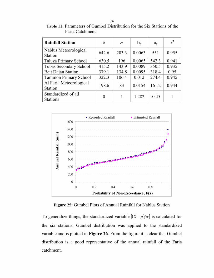
74 Table 11: Parameters of Gumbel Distribution for the Six Stations of the
Faria Catchment
0
200
400
600
800
1000
1200
1400
1600
0 0.2 0.4 0.6 0.8 1
Probability of Non-Exceedance, F(x)
Ann
ual R
ainf
all (
mm
)
Recorded Rainfall Estimated Rainfall
Figure 25: Gumbel Plots of Annual Rainfall for Nablus Station
To generalize things, the standardized variable ( )[ ]σμ−X is calculated for
the six stations. Gumbel distribution was applied to the standardized
variable and is plotted in Figure 26. From the figure it is clear that Gumbel
distribution is a good representative of the annual rainfall of the Faria
catchment.
Rainfall Station μ σ bg ag r2 Nablus Meteorological Station 642.6 203.3 0.0063 551 0.955
Taluza Primary School 630.5 196 0.0065 542.3 0.941Tubas Secondary School 415.2 143.9 0.0089 350.5 0.935 Beit Dajan Station 379.1 134.8 0.0095 318.4 0.95 Tammon Primary School 322.3 106.4 0.012 274.4 0.945 Al Faria Meteorological Station 198.6 83 0.0154 161.2 0.944
Standardized of all Stations 0 1 1.282 -0.45 1
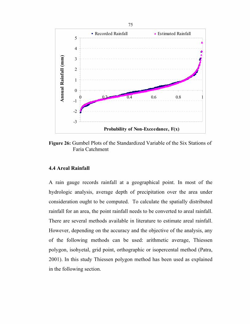
75
-3
-2
-1
0
1
2
3
4
5
0 0.2 0.4 0.6 0.8 1
Probability of Non-Exceedance, F(x)
Ann
ual R
ainf
all (
mm
)
Recorded Rainfall Estimated Rainfall
Figure 26: Gumbel Plots of the Standardized Variable of the Six Stations of Faria Catchment
4.4 Areal Rainfall
A rain gauge records rainfall at a geographical point. In most of the
hydrologic analysis, average depth of precipitation over the area under
consideration ought to be computed. To calculate the spatially distributed
rainfall for an area, the point rainfall needs to be converted to areal rainfall.
There are several methods available in literature to estimate areal rainfall.
However, depending on the accuracy and the objective of the analysis, any
of the following methods can be used: arithmetic average, Thiessen
polygon, isohyetal, grid point, orthographic or isopercental method (Patra,
2001). In this study Thiessen polygon method has been used as explained
in the following section.
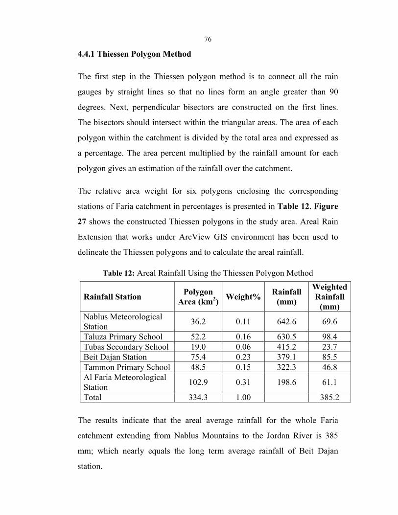
76
4.4.1 Thiessen Polygon Method
The first step in the Thiessen polygon method is to connect all the rain
gauges by straight lines so that no lines form an angle greater than 90
degrees. Next, perpendicular bisectors are constructed on the first lines.
The bisectors should intersect within the triangular areas. The area of each
polygon within the catchment is divided by the total area and expressed as
a percentage. The area percent multiplied by the rainfall amount for each
polygon gives an estimation of the rainfall over the catchment.
The relative area weight for six polygons enclosing the corresponding
stations of Faria catchment in percentages is presented in Table 12. Figure
27 shows the constructed Thiessen polygons in the study area. Areal Rain
Extension that works under ArcView GIS environment has been used to
delineate the Thiessen polygons and to calculate the areal rainfall.
Table 12: Areal Rainfall Using the Thiessen Polygon Method
Rainfall Station Polygon Area (km2) Weight% Rainfall
(mm)
Weighted Rainfall
(mm) Nablus Meteorological Station 36.2 0.11 642.6 69.6
Taluza Primary School 52.2 0.16 630.5 98.4 Tubas Secondary School 19.0 0.06 415.2 23.7 Beit Dajan Station 75.4 0.23 379.1 85.5 Tammon Primary School 48.5 0.15 322.3 46.8 Al Faria Meteorological Station 102.9 0.31 198.6 61.1
Total 334.3 1.00 385.2
The results indicate that the areal average rainfall for the whole Faria
catchment extending from Nablus Mountains to the Jordan River is 385
mm; which nearly equals the long term average rainfall of Beit Dajan
station.
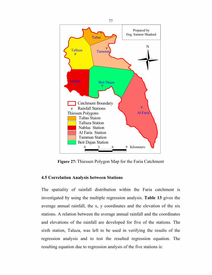
77
#Y
#Y
#Y
#Y
#Y
#Y
Tubas
Nablus
Tammun
Al-Faria
Talluza
Beit Dajan
N
Prepared byEng. Sameer Shadeed
Thiessen Polygons Tubas Staion Talluza Station Nablus Station Al Faria Station Tammun StationBeit Dajan Station
#Y Rainfall StationsCatchment Boundary
0 3 6 9 Kilometers
Figure 27: Thiessen Polygon Map for the Faria Catchment
4.5 Correlation Analysis between Stations
The spatiality of rainfall distribution within the Faria catchment is
investigated by using the multiple regression analysis. Table 13 gives the
average annual rainfall, the x, y coordinates and the elevation of the six
stations. A relation between the average annual rainfall and the coordinates
and elevations of the rainfall are developed for five of the stations. The
sixth station, Taluza, was left to be used in verifying the results of the
regression analysis and to test the resulted regression equation. The
resulting equation due to regression analysis of the five stations is:
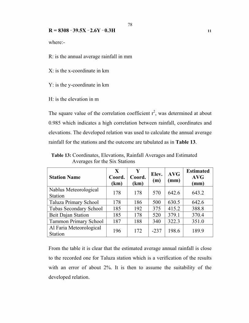
78R = 8308 _ 39.5X _ 2.6Y _ 0.3H 11
where:-
R: is the annual average rainfall in mm
X: is the x-coordinate in km
Y: is the y-coordinate in km
H: is the elevation in m
The square value of the correlation coefficient r2, was determined at about
0.985 which indicates a high correlation between rainfall, coordinates and
elevations. The developed relation was used to calculate the annual average
rainfall for the stations and the outcome are tabulated as in Table 13.
Table 13: Coordinates, Elevations, Rainfall Averages and Estimated Averages for the Six Stations
From the table it is clear that the estimated average annual rainfall is close
to the recorded one for Taluza station which is a verification of the results
with an error of about 2%. It is then to assume the suitability of the
developed relation.
Station Name X
Coord. (km)
Y Coord.(km)
Elev.(m)
AVG (mm)
Estimated AVG (mm)
Nablus Meteorological Station 178 178 570 642.6 643.2
Taluza Primary School 178 186 500 630.5 642.6 Tubas Secondary School 185 192 375 415.2 388.8 Beit Dajan Station 185 178 520 379.1 370.4 Tammon Primary School 187 188 340 322.3 351.0 Al Faria Meteorological Station 196 172 -237 198.6 189.9

79
CHAPTER FIVE
RUNOFF MODELING
80
5.1 Introduction
The computation of flow hydrograph is of great importance to water
resources engineers and scientists. Among the most basic challenges of
hydrology are the quantitative understanding of the processes of runoff
generation and prediction of the flow hydrographs and their transmission to
the outlet. The high spatial variability in rainfall intensities and amounts
combined with variability in soil properties makes prediction of runoff
generation very difficult especially for ungauged catchments. Even in cases
where catchments are gauged, the period of record is often too short to
allow accurate estimates of the different hydraulic parameters.
Traditional techniques have been widely applied for the estimation of
runoff hydrographs at the outlets of gauged catchments using historical
rainfall runoff data and unit hydrographs derived from them. Such
procedures are questioned for their reliability due to the climatic and
physical changes in the catchment and their application to ungauged, arid
and semiarid catchments.
In the unit hydrograph theory it is assumed that the potential abstractions
are fully met before runoff occurs. This assumption is applicable to humid
regions, but is doubtful in arid and semiarid regions. For arid and semiarid
regions, the infiltration portion is higher than for humid regions due to
higher infiltration rates and dry soil antecedent moisture condition. The
infiltrability of the soil is high and the infiltration process will continue
significantly during the rainfall event. The amount of actual infiltration
may not satisfy the infiltrability of the soil. The evaporation losses are also
high in arid and semiarid regions and the evaporation process may occur
during the storm. Therefore the applicability of the unit hydrograph
81
approach in semiarid regions should be investigated as to its basic
assumption of satisfying the abstraction and neglecting the surface and
subsurface flow interaction during the rainfall-runoff process (Shaheen,
2001).
In the West Bank, which is characterized as semiarid region, hydrological
modeling has not been given enough care and no intensive studies have
been done. However, this study is an attempt to hydrologically investigate
and to derive the unit hydrograph for the Faria catchment as one of the
most important catchments of the West Bank, since the catchment has not
been modeled using appropriate rainfall-runoff model so far. The KW-
GIUH model that was developed for ungauged catchments is to be used in
the modeling.
5.2 GIUH Model
Hydrological simulation models can take the form of theoretical linkage
between the geomorphology and hydrology. The geomorphological
instantaneous unit hydrograph (GIUH) is one approach of these kinds of
models. The GIUH focuses on finding the catchment response given its
geomorphological features. The model uses catchment characteristics to
predict flow rates. GIUH can be applied to any excess rainfall through
convolution to produce the direct runoff hydrograph.
GIUH approach has been applied by several engineers to predict runoff
from rainfall for ungauged catchments. They have been proposed to
estimate floods for ungauged streams by using the information obtainable
from topographic maps or remote sensing possibly linked with the
82
Geographic Information Systems (GIS) and Digital Elevation Models
(DEM) (Snell and Sivapalan, 1994; Jain et al., 2000; and Hall et al., 2001).
Lee and Chang (2005) reviewed the development of GIUH approach and
concluded that the significant advance in research on the topographic
runoff approaches was the development of the geomorphologic
instantaneous unit hydrograph model (GIUH) proposed by Rodriguez-
Iturbe and Valdes (1979). During the last two decades, the use of
catchment geomorphologic characteristics in runoff simulations has
received a great deal of attention from hydrologists (e.g. Gupta et al., 1980;
Rodriguez-Iturbe et al., 1982; Kirshen and Bras, 1983; Karlinger and
Troutman, 1985; Agnese et al., 1988; Chutha and Dooge, 1990; Lee and
Yen, 1997; Yen and Lee, 1997; Olivera and Maidment, 1999; Berod et al.,
1999; Brooks and McDonnell, 2000).
The concept of the Geomorphological unit hydrograph is introduced by
Rodriguez-Iturbe and Valdes in 1979. This method is based on the Horton-
Strahler ordering law.
In the Strahler system for stream ordering and catchment ranking a stream
segment with no tributaries is called a first order segment. When two
stream segments of the same order meet, the order of the downstream
stream segment is raised with one. When two stream segments of a
different order meet, the order of the downstream segment is equal to the
highest order upstream.
In the GIUH approach, Rainfall excess is assumed to follow different paths
on overland areas and in channels of different stream orders
probabilistically, according to the drainage pattern to reach the catchment
outlet. The travel time of the rainfall excess is assumed to follow a
83
probability distribution in a channel of a given order. The exponential and
uniform distributions have been proposed by Gupta et al. (1980). Jin
(1992) suggested gamma distribution to get better results. Various methods
have been used to determine the time scale to be used with the probability
distribution. Rodriguez-Iturbe and Valdes (1979) gave the time parameters
as regression equations from discharge records. Agnese et al. (1988)
obtained the time scale formula from experimental data. Rodriguez-Iturbe
et al. (1982) estimated the first order channel travel time by using a
kinematic wave approximation. The travel times of higher order channels
were then related to the first order channels through geomorphologic laws.
An alternative approach was provided by Lee and Yen (1997). The travel
times for different orders of overland areas and channels were derived
using the kinematic wave theory and then substituted into the GIUH model
to develop a kinematic wave based GIUH model (KW-GIUH) for
catchment runoff simulation. The available KW-GIUH program (version
1.2) can be applied to catchments with stream network of up to the seventh
order. The program has been developed by Kwan Tun Lee and Chin-Hisn
Chang, Watershed Hydrology and Hydraulics Laboratory, Department of
River and Harbor Engineering and National Taiwan Ocean University. The
KW-GIUH model is applied in this study to predict the runoff hydrographs
of the Faria catchment.
5.3 Travel Time Estimation of the KW-GIUH Model
The travel time of the surface flow on a hillslope depends on the slope,
surface roughness, and flow depth. The travel times for different orders of
overland areas and channels were derived using the kinematic-wave theory
and then substituted into the GIUH model to develop a kinematic-wave
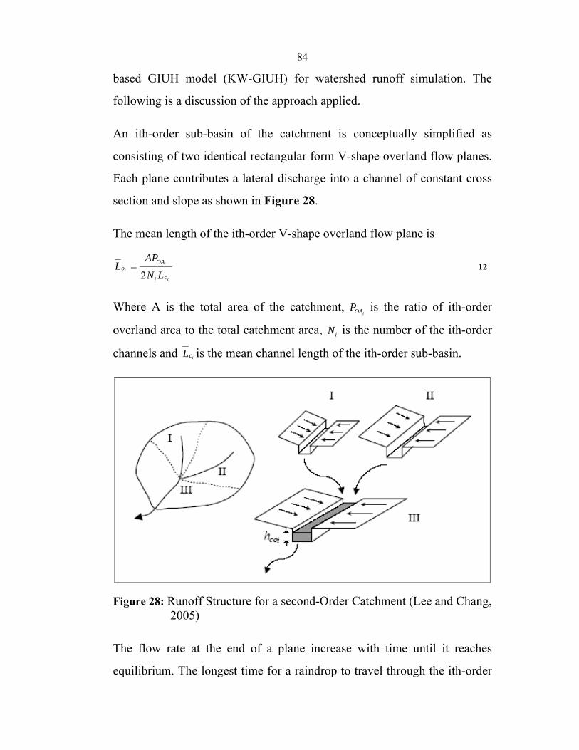
84
based GIUH model (KW-GIUH) for watershed runoff simulation. The
following is a discussion of the approach applied.
An ith-order sub-basin of the catchment is conceptually simplified as
consisting of two identical rectangular form V-shape overland flow planes.
Each plane contributes a lateral discharge into a channel of constant cross
section and slope as shown in Figure 28.
The mean length of the ith-order V-shape overland flow plane is
c
ii
ci
OAo
LNAP
L2
= 12
Where A is the total area of the catchment, iOAP is the ratio of ith-order
overland area to the total catchment area, iN is the number of the ith-order
channels and icL is the mean channel length of the ith-order sub-basin.
Figure 28: Runoff Structure for a second-Order Catchment (Lee and Chang, 2005)
The flow rate at the end of a plane increase with time until it reaches
equilibrium. The longest time for a raindrop to travel through the ith-order

85
overland plane oixT is the time for the flow to reach equilibrium in the plane.
Thus, the discharge for the ith-order overland sub-basin at any time, oixTt < ,
is
mL
o
oo tq
nSq i
i)(
21
= 13
Where ioq is the ith-order overland flow discharge per unit width, ioS is the
mean ith-order overland slope, on is the overland flow roughness
coefficient, m is a constant and Lq is the lateral flow rate joining the main
flowioq .
Once the flow equilibrium state reached, the discharge afterward, oixTt > , is
mos
o
ooLoso i
iii
hn
SLqqq21
1=== 14
Where iosq and
iosh represent the ith-order overland discharge and water
depth at equilibrium, respectively. The travel time for the ith-order
overland plane is m
mLo
oo
L
osx
qS
Lnqh
Ti
ii
oi
1
121 ⎟⎟
⎠
⎞
⎜⎜
⎝
⎛==
− 15
Since the sub-basin model is conceptually composed of two identical
rectangular planes, the lateral discharge into the central channel is
contributed from both side planes. Thus, the lateral discharge
becomes ioL Lq2 . The amount of rain that falls directly onto the channels is
small compared to that falling on overland planes and can therefore be
neglected. As the flow in the ith-order overland planes gradually increases with time to reach equilibrium, an additional time
ixT is needed for the ith-
order channel to reach its equilibrium. A first order channel conveys only
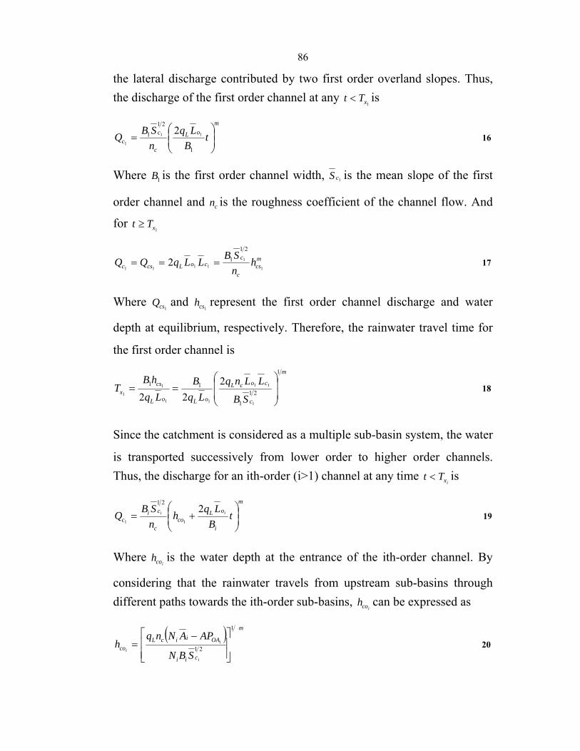
86
the lateral discharge contributed by two first order overland slopes. Thus, the discharge of the first order channel at any
1xTt < is
moL
c
cc t
BLq
nSBQ ⎟
⎟⎠
⎞⎜⎜⎝
⎛=
1
21
1 11
1
2 16
Where 1B is the first order channel width, 1cS is the mean slope of the first
order channel and cn is the roughness coefficient of the channel flow. And
for 1xTt ≥
mcs
c
ccoLcsc h
nSBLLqQQ
1
11111
21
12 === 17
Where 1csQ and
1csh represent the first order channel discharge and water
depth at equilibrium, respectively. Therefore, the rainwater travel time for
the first order channel is m
c
cocL
oLoL
csx
SB
LLnqLq
BLq
hBT
1
21
1
11
1
11
11
1
1
222 ⎟
⎟
⎠
⎞
⎜⎜
⎝
⎛== 18
Since the catchment is considered as a multiple sub-basin system, the water
is transported successively from lower order to higher order channels. Thus, the discharge for an ith-order (i>1) channel at any time
ixTt < is
m
i
oLco
c
cic t
BLqh
nSBQ ii
⎟⎟⎠
⎞⎜⎜⎝
⎛+=
211
21
19
Where icoh is the water depth at the entrance of the ith-order channel. By
considering that the rainwater travels from upstream sub-basins through different paths towards the ith-order sub-basins,
icoh can be expressed as
( ) m
cii
OAiicLco
i
i
i SBN
APANnqh
1
21⎥⎥⎦
⎤
⎢⎢⎣
⎡ −= 20
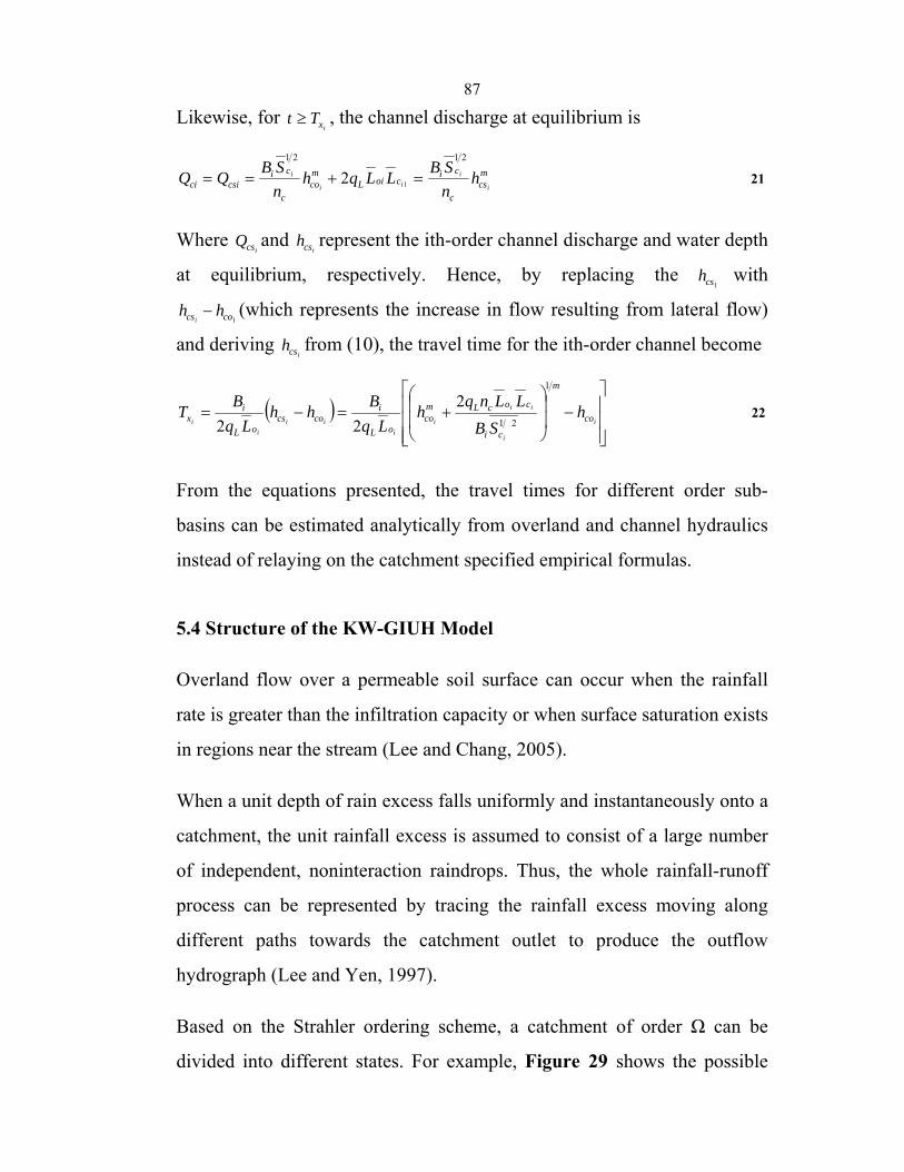
87
Likewise, for ixTt ≥ , the channel discharge at equilibrium is
mcs
c
cicoiL
mco
c
cicsici i
iii
i hnSBLLqh
nSBQQ
2121
12 =+== 21
Where icsQ and
icsh represent the ith-order channel discharge and water depth
at equilibrium, respectively. Hence, by replacing the 1csh with
1cocs hhi− (which represents the increase in flow resulting from lateral flow)
and deriving icsh from (10), the travel time for the ith-order channel become
( )⎥⎥⎥
⎦
⎤
⎢⎢⎢
⎣
⎡−⎟
⎟
⎠
⎞
⎜⎜
⎝
⎛+=−=
i
i
ii
ii
iii
i co
m
ci
cocLmco
oL
icocs
oL
ix h
SBLLnqh
LqBhh
LqBT
1
21
222
22
From the equations presented, the travel times for different order sub-
basins can be estimated analytically from overland and channel hydraulics
instead of relaying on the catchment specified empirical formulas.
5.4 Structure of the KW-GIUH Model
Overland flow over a permeable soil surface can occur when the rainfall
rate is greater than the infiltration capacity or when surface saturation exists
in regions near the stream (Lee and Chang, 2005).
When a unit depth of rain excess falls uniformly and instantaneously onto a
catchment, the unit rainfall excess is assumed to consist of a large number
of independent, noninteraction raindrops. Thus, the whole rainfall-runoff
process can be represented by tracing the rainfall excess moving along
different paths towards the catchment outlet to produce the outflow
hydrograph (Lee and Yen, 1997).
Based on the Strahler ordering scheme, a catchment of order Ω can be
divided into different states. For example, Figure 29 shows the possible
88
travel paths of the rain drops for a third-order catchment. Most of the
surface flow occurs on the low portions of the catchment (the shaded area
in Figure 29); after that, it goes into the adjacent channel and then flows
through the stream network to the outlet. Each raindrop falling on the
overland region will move successively from lower to higher order
channels until it reaches the outlet. The catchment geomorphology is
represented probabilistically based on the stream order, instead of
simulating the overland surfaces and channels by their individually actual
geometry as in the deterministic modeling. The ith-order overland regions
is denoted by xoi and xi represents the ith-order channel, in which i = 1, 2,…, Ω. If w denotes a specified runoff path Ω→→→→ xxxx jioi ..... ,the
probability of a drop of rainfall excess adopting this path can be expressed
as
( ) . ... ...i oi i i j kOA x x x x x xP w P P P P
Ω= ,where
ioi xxP is the transitional probability of the
raindrop moving from the ith-order overland region to the ith-order channel and ji xxP is the transitional probability of the raindrop moving from an ith-
order channel to a jth-order channel and is computed as
i
jixx N
NP
ji
,= 23
Where ijN is the number of ith-order channels contributing to the jth-order
channels and iOAP is the ratio of ith-order overland area to the total
catchment and is computed as
⎟⎠
⎞⎜⎝
⎛−= ∑
−
=jii xx
i
iiiiOA PANAN
AP
1
1
1 24
Where iA is the mean of the drainage area of order i. and is estimated as
89
∑=
=iN
jji
i
i AN
A1
1 25
It should be noted that Aji denotes not only the areas of the overland flow
regions that drains directly into the jth channel of order i, but it also
includes overland areas draining into the lower order channels tributary to
this jth channel of order i.
The travel time for the overland flow region and for the storage component
of a channel are assumed to follow an exponential distribution, but the
translation component of a channel is assumed to follow a uniform distribution. For the state kx , the travel time for the channel storage
component and channel translation component are rkxT and
ckxT , respectively,
and the total travel time is ckrkk xxx TTT +=
The IUH can be represented by the convolution of two groups of the
probability density functions and is given by:
[ ] [ ] )(.)(*.....*)(*)(*)(*.....*)(*)(*)()( wPtftftftftftftftuw
xxxxxxx ccjcirrjrioi∑ ΩΩ= 26
The first part of equation (25) represents the overland flow region )( okx and
the channel storage component )( rkx . The exponential distribution with a
mean travel time of kxT is
⎟⎟⎠
⎞⎜⎜⎝
⎛ −=
kk
kxx
x Tt
Ttf exp1)( , for all t 27
The second part of equation (25) represents the channel translation component )( ckx . The uniform distribution with a men travel time of
kxT over an interval (0, 2 kxT ) is
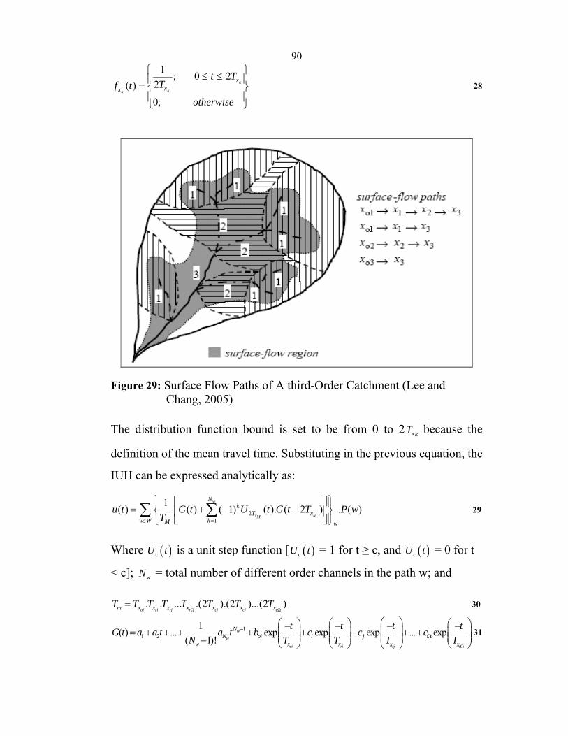
90
⎪⎭
⎪⎬
⎫
⎪⎩
⎪⎨
⎧ ≤≤=
otherwise
TtTtf k
kk
xxx
;0
20;2
1)( 28
Figure 29: Surface Flow Paths of A third-Order Catchment (Lee and Chang, 2005)
The distribution function bound is set to be from 0 to 2 kxT because the
definition of the mean travel time. Substituting in the previous equation, the
IUH can be expressed analytically as:
21
1( ) ( ) ( 1) ( ). ( 2 ) . ( )w
x MM
Nk
T xw W kM w
u t G t U t G t T P wT∈ =
⎧ ⎫⎡ ⎤⎪ ⎪= + − −⎨ ⎬⎢ ⎥⎪ ⎪⎣ ⎦⎩ ⎭
∑ ∑ 29
Where ( )cU t is a unit step function [ ( )cU t = 1 for t ≥ c, and ( )cU t = 0 for t
< c]; wN = total number of different order channels in the path w; and
. . ... .(2 ).(2 )...(2 )oi ri rj r ci cj cm x x x x x x xT T T T T T T T
Ω Ω= 30
1
1 21( ) ... exp exp exp ... exp
( 1)!w
w
oi ri rj r
NN oi i j
w x x x x
t t t tG t a a t a t b c c cN T T T T
Ω
−Ω
⎛ ⎞⎛ ⎞ ⎛ ⎞ ⎛ ⎞− − − −⎜ ⎟= + + + + + + + +⎜ ⎟ ⎜ ⎟ ⎜ ⎟⎜ ⎟⎜ ⎟ ⎜ ⎟ ⎜ ⎟− ⎝ ⎠⎝ ⎠ ⎝ ⎠ ⎝ ⎠ 31

91
Ω∈= cckcjcickcjciM xxxxxxxX ,.....,,....,,,....,, 32
1M ci
M
x xi
T T=
= ∑ 33
Where M denotes the size of MX ; and 1 2, ,..., , , , ,..., .wN oi i ja a a b c c c coefficientsΩ =
The coefficients are determined by comparing coefficients in partial fractions
after applying the Laplace transformation.
5.5 KW-GIUH Model Input Parameters
In the following sections the input parameters for the application of the
KW-GIUH model on the Faria catchment.
5.5.1 Hydraulic parameters
The following notations are used
• Catchment area (km2)
• Rainfall duration (hr)
• Flow duration (hr)
• Baseflow (m3/s) or Φ index (mm/hr)
• Hourly rainfall intensity i (mm/hr)
• Hourly discharge (m3/s)
5.5.2 Geomorphic parameters
• Stream network order Ω
92
• Overland flow roughness on
• Channel flow roughness cn
• ith-order stream number Ni
• Mean ith-order stream length L ic (km)
• ith-order sub catchment contributing area Ai (km2)
• Ratio of ith-order overland area to the catchment area P i OA
• Mean ith-order overland slope S io (m/m)
• Mean ith-order channel slope S ic (m/m)
• Stream network transitional probability ji xxP
• Channel width at catchment outlet ΩB (m)
5.5.3 Parameter Estimation Using GIS
The Geographical Information System (GIS) techniques were used to shape
the geomorphological features of the catchment. In this study, GIS
ArcView 3.2 software was used for geomorphological parameter
determinations. The catchment stream networks, sub-catchments area,
stream lengths and others were produced by using 1:50,000 scanned
topography map under the GIS environment. A Digital Elevations Model
(DEM) with a 20-m resolution has been used to derive flow directions and
stream slopes. The DEM of the Faria catchment is shown in Figure 30. The
hydraulic parameters have been derived from the available rainfall and
runoff data.
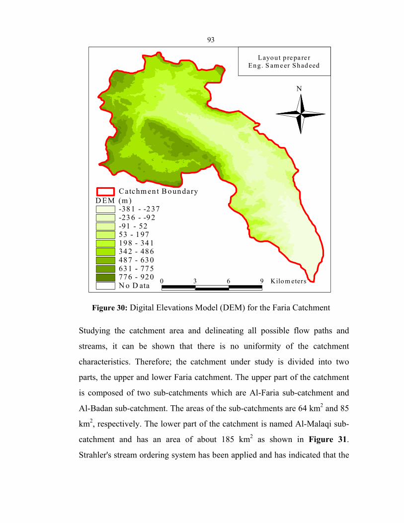
93
N
Layout p repa re rEng . S ameer Shadeed
D EM (m )-38 1 - -2 37-23 6 - -9 2-91 - 5253 - 1 97198 - 34 1342 - 48 6487 - 63 0631 - 77 5776 - 92 0N o D ata
Catchm en t B oun dary
0 3 6 9 Kilom eters
Figure 30: Digital Elevations Model (DEM) for the Faria Catchment
Studying the catchment area and delineating all possible flow paths and
streams, it can be shown that there is no uniformity of the catchment
characteristics. Therefore; the catchment under study is divided into two
parts, the upper and lower Faria catchment. The upper part of the catchment
is composed of two sub-catchments which are Al-Faria sub-catchment and
Al-Badan sub-catchment. The areas of the sub-catchments are 64 km2 and 85
km2, respectively. The lower part of the catchment is named Al-Malaqi sub-
catchment and has an area of about 185 km2 as shown in Figure 31.
Strahler's stream ordering system has been applied and has indicated that the
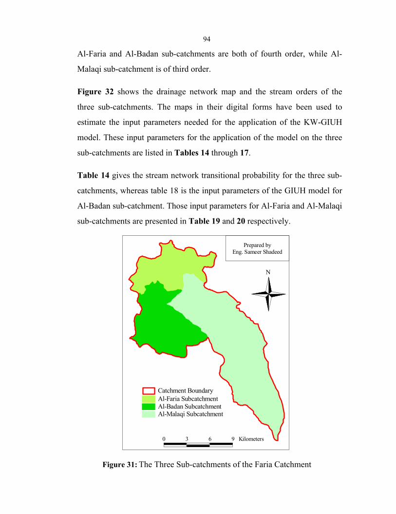
94
Al-Faria and Al-Badan sub-catchments are both of fourth order, while Al-
Malaqi sub-catchment is of third order.
Figure 32 shows the drainage network map and the stream orders of the
three sub-catchments. The maps in their digital forms have been used to
estimate the input parameters needed for the application of the KW-GIUH
model. These input parameters for the application of the model on the three
sub-catchments are listed in Tables 14 through 17.
Table 14 gives the stream network transitional probability for the three sub-
catchments, whereas table 18 is the input parameters of the GIUH model for
Al-Badan sub-catchment. Those input parameters for Al-Faria and Al-Malaqi
sub-catchments are presented in Table 19 and 20 respectively.
N
Prepared byEng. Sameer Shadeed
Al-Malaqi SubcatchmentAl-Badan SubcatchmentAl-Faria SubcatchmentCatchment Boundary
0 3 6 9 Kilometers
Figure 31: The Three Sub-catchments of the Faria Catchment
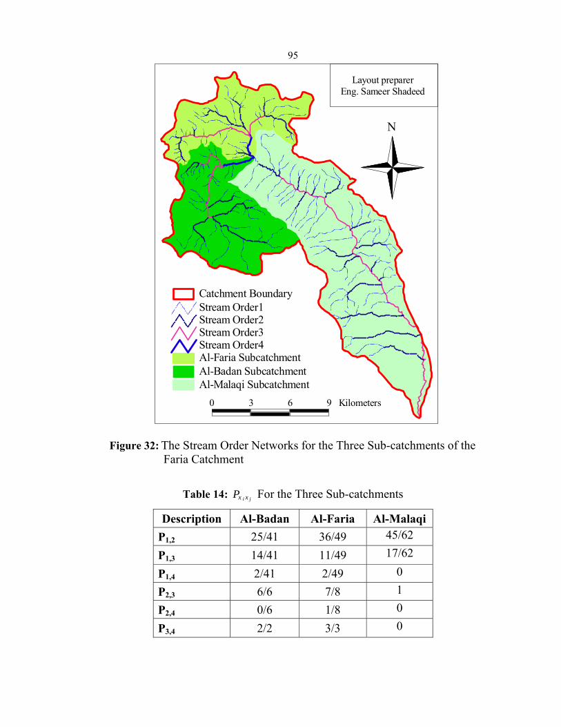
95
N
Layout preparerEng. Sameer Shadeed
0 3 6 9 Kilometers
Al-Malaqi SubcatchmentAl-Badan SubcatchmentAl-Faria SubcatchmentStream Order4Stream Order3Stream Order2Stream Order1Catchment Boundary
Figure 32: The Stream Order Networks for the Three Sub-catchments of the Faria Catchment
Table 14: ji xxP For the Three Sub-catchments
Description Al-Badan Al-Faria Al-Malaqi P1,2 25/41 36/49 45/62
P1,3 14/41 11/49 17/62
P1,4 2/41 2/49 0
P2,3 6/6 7/8 1
P2,4 0/6 1/8 0
P3,4 2/2 3/3 0
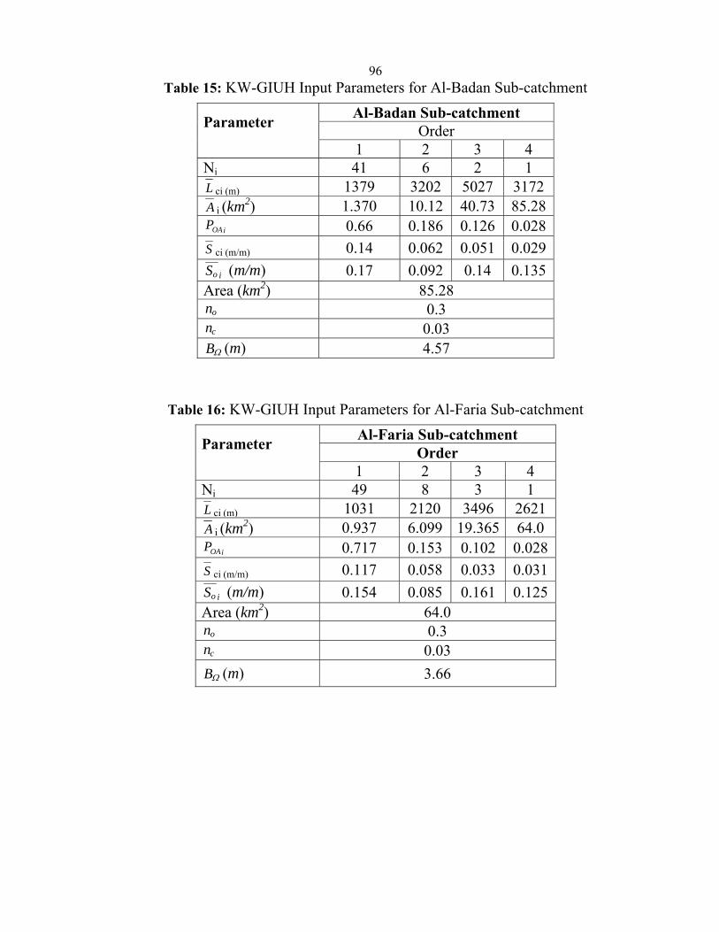
96Table 15: KW-GIUH Input Parameters for Al-Badan Sub-catchment
Parameter
Al-Badan Sub-catchment Order
1 2 3 4 Ni 41 6 2 1 L ci (m) 1379 3202 5027 3172 A i (km2) 1.370 10.12 40.73 85.28
iOAP 0.66 0.186 0.126 0.028 S ci (m/m) 0.14 0.062 0.051 0.029
S io (m/m) 0.17 0.092 0.14 0.135 Area (km2) 85.28
on 0.3 cn 0.03 ΩB (m) 4.57
Table 16: KW-GIUH Input Parameters for Al-Faria Sub-catchment
Parameter
Al-Faria Sub-catchment Order
1 2 3 4 Ni 49 8 3 1 L ci (m) 1031 2120 3496 2621 A i (km2) 0.937 6.099 19.365 64.0
iOAP 0.717 0.153 0.102 0.028 S ci (m/m) 0.117 0.058 0.033 0.031
S io (m/m) 0.154 0.085 0.161 0.125 Area (km2) 64.0
on 0.3 cn 0.03 ΩB (m) 3.66

97Table 17: KW-GIUH Input Parameters for Al-Malaqi Sub-catchment
Parameter
Al-Malaqi Sub-catchment Order
1 2 3 Ni 62 16 1 L ci (m) 1920 2611 32084 A i (km2) 1.81 5.83 184.96
iOAP 0.606 0.319 0.075 S ci (m/m) 0.14 0.063 0.01
S io (m/m) 0.146 0.122 0.081 Area (km2) 184.96
on 0.3 cn 0.03 ΩB (m) 10
5.6 KW-GIUH Unit Hydrograph Derivation
For the analysis of the Faria catchment and the development of the 1-hr
unit hydrograph for Al-Badan, Al-Faria and Al-Malaqi sub-catchments, the
following are assumed.
• Rainfall duration = 1 hr
• Flow duration, there is no gauging for discharge
• Φ index = 0.0 mm/hr
• Hourly rainfall intensity i = 1 mm/hr
• Overland and channel flow roughness on and cn were estimated
depending upon the features of the catchment and based on the model
verification as discussed in section 5.7.
The computer outputs for the three sub-catchments resulting from applying
the KW-GIUH model are presented in Appendix C. From the outputs the
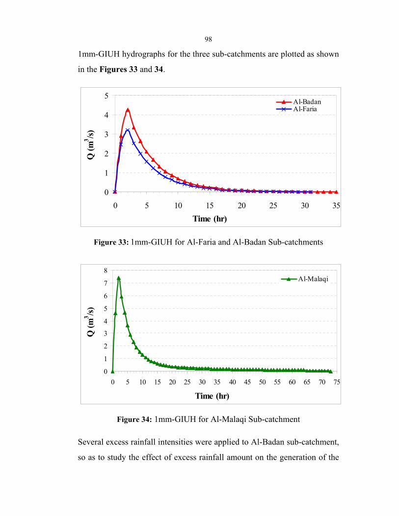
98
1mm-GIUH hydrographs for the three sub-catchments are plotted as shown
in the Figures 33 and 34.
0
1
2
3
4
5
0 5 10 15 20 25 30 35Time (hr)
Q (m
3 /s)Al-BadanAl-Faria
Figure 33: 1mm-GIUH for Al-Faria and Al-Badan Sub-catchments
0
1
2
3
4
5
6
7
8
0 5 10 15 20 25 30 35 40 45 50 55 60 65 70 75
Time (hr)
Q (m
3 /s)
Al-Malaqi
Figure 34: 1mm-GIUH for Al-Malaqi Sub-catchment
Several excess rainfall intensities were applied to Al-Badan sub-catchment,
so as to study the effect of excess rainfall amount on the generation of the
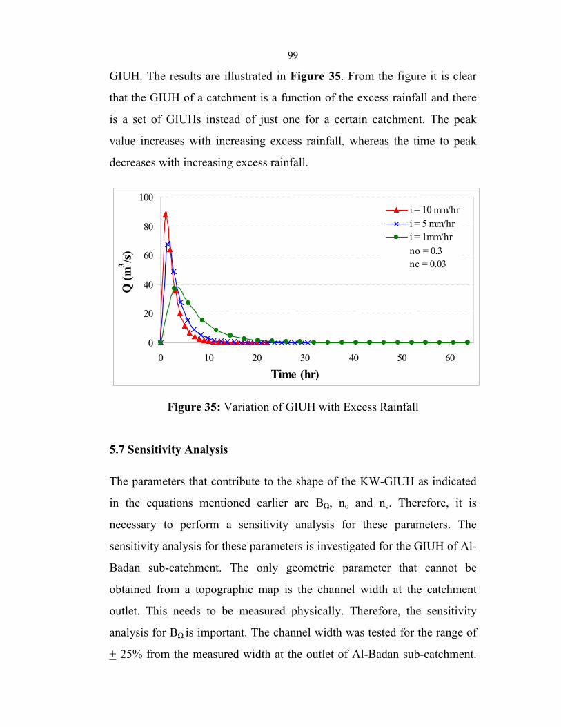
99
GIUH. The results are illustrated in Figure 35. From the figure it is clear
that the GIUH of a catchment is a function of the excess rainfall and there
is a set of GIUHs instead of just one for a certain catchment. The peak
value increases with increasing excess rainfall, whereas the time to peak
decreases with increasing excess rainfall.
0
20
40
60
80
100
0 10 20 30 40 50 60
Time (hr)
Q (m
3 /s)
i = 10 mm/hri = 5 mm/hri = 1mm/hrno = 0.3nc = 0.03
Figure 35: Variation of GIUH with Excess Rainfall
5.7 Sensitivity Analysis
The parameters that contribute to the shape of the KW-GIUH as indicated
in the equations mentioned earlier are BΩ, no and nc. Therefore, it is
necessary to perform a sensitivity analysis for these parameters. The
sensitivity analysis for these parameters is investigated for the GIUH of Al-
Badan sub-catchment. The only geometric parameter that cannot be
obtained from a topographic map is the channel width at the catchment
outlet. This needs to be measured physically. Therefore, the sensitivity
analysis for BΩ is important. The channel width was tested for the range of
+ 25% from the measured width at the outlet of Al-Badan sub-catchment.
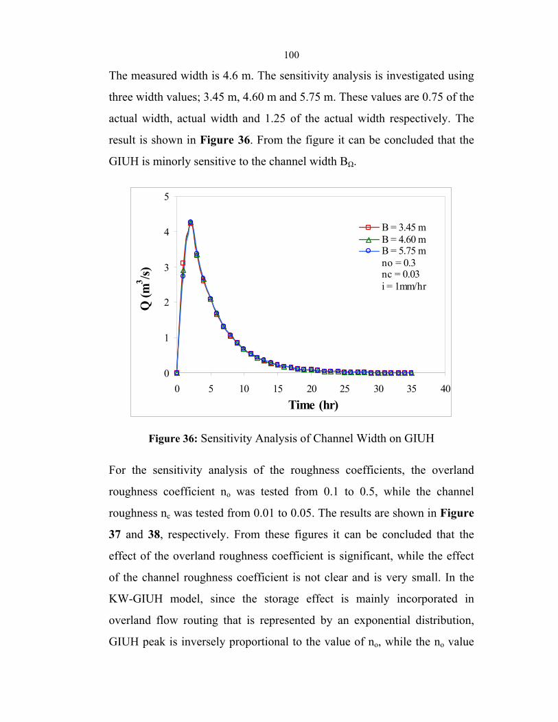
100
The measured width is 4.6 m. The sensitivity analysis is investigated using
three width values; 3.45 m, 4.60 m and 5.75 m. These values are 0.75 of the
actual width, actual width and 1.25 of the actual width respectively. The
result is shown in Figure 36. From the figure it can be concluded that the
GIUH is minorly sensitive to the channel width BΩ.
0
1
2
3
4
5
0 5 10 15 20 25 30 35 40Time (hr)
Q (m
3 /s)
B = 3.45 mB = 4.60 mB = 5.75 mno = 0.3nc = 0.03i = 1mm/hr
Figure 36: Sensitivity Analysis of Channel Width on GIUH
For the sensitivity analysis of the roughness coefficients, the overland
roughness coefficient no was tested from 0.1 to 0.5, while the channel
roughness nc was tested from 0.01 to 0.05. The results are shown in Figure
37 and 38, respectively. From these figures it can be concluded that the
effect of the overland roughness coefficient is significant, while the effect
of the channel roughness coefficient is not clear and is very small. In the
KW-GIUH model, since the storage effect is mainly incorporated in
overland flow routing that is represented by an exponential distribution,
GIUH peak is inversely proportional to the value of no, while the no value
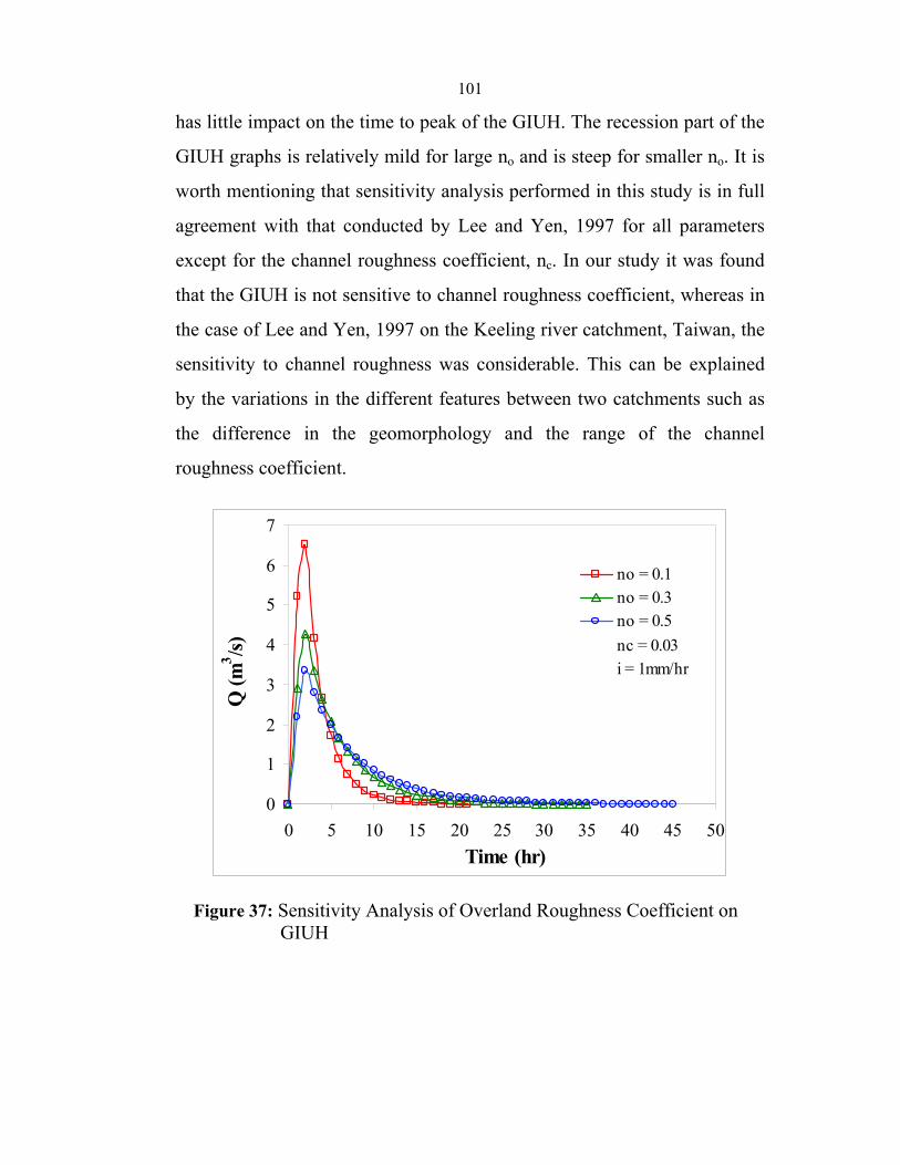
101
has little impact on the time to peak of the GIUH. The recession part of the
GIUH graphs is relatively mild for large no and is steep for smaller no. It is
worth mentioning that sensitivity analysis performed in this study is in full
agreement with that conducted by Lee and Yen, 1997 for all parameters
except for the channel roughness coefficient, nc. In our study it was found
that the GIUH is not sensitive to channel roughness coefficient, whereas in
the case of Lee and Yen, 1997 on the Keeling river catchment, Taiwan, the
sensitivity to channel roughness was considerable. This can be explained
by the variations in the different features between two catchments such as
the difference in the geomorphology and the range of the channel
roughness coefficient.
0
1
2
3
4
5
6
7
0 5 10 15 20 25 30 35 40 45 50Time (hr)
Q (m
3 /s)
no = 0.1no = 0.3no = 0.5nc = 0.03i = 1mm/hr
Figure 37: Sensitivity Analysis of Overland Roughness Coefficient on GIUH
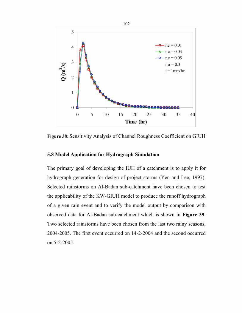
102
0
1
2
3
4
5
0 5 10 15 20 25 30 35 40Time (hr)
Q (m
3 /s)
nc = 0.01nc = 0.03nc = 0.05no = 0.3i = 1mm/hr
Figure 38: Sensitivity Analysis of Channel Roughness Coefficient on GIUH
5.8 Model Application for Hydrograph Simulation
The primary goal of developing the IUH of a catchment is to apply it for
hydrograph generation for design of project storms (Yen and Lee, 1997).
Selected rainstorms on Al-Badan sub-catchment have been chosen to test
the applicability of the KW-GIUH model to produce the runoff hydrograph
of a given rain event and to verify the model output by comparison with
observed data for Al-Badan sub-catchment which is shown in Figure 39.
Two selected rainstorms have been chosen from the last two rainy seasons,
2004-2005. The first event occurred on 14-2-2004 and the second occurred
on 5-2-2005.
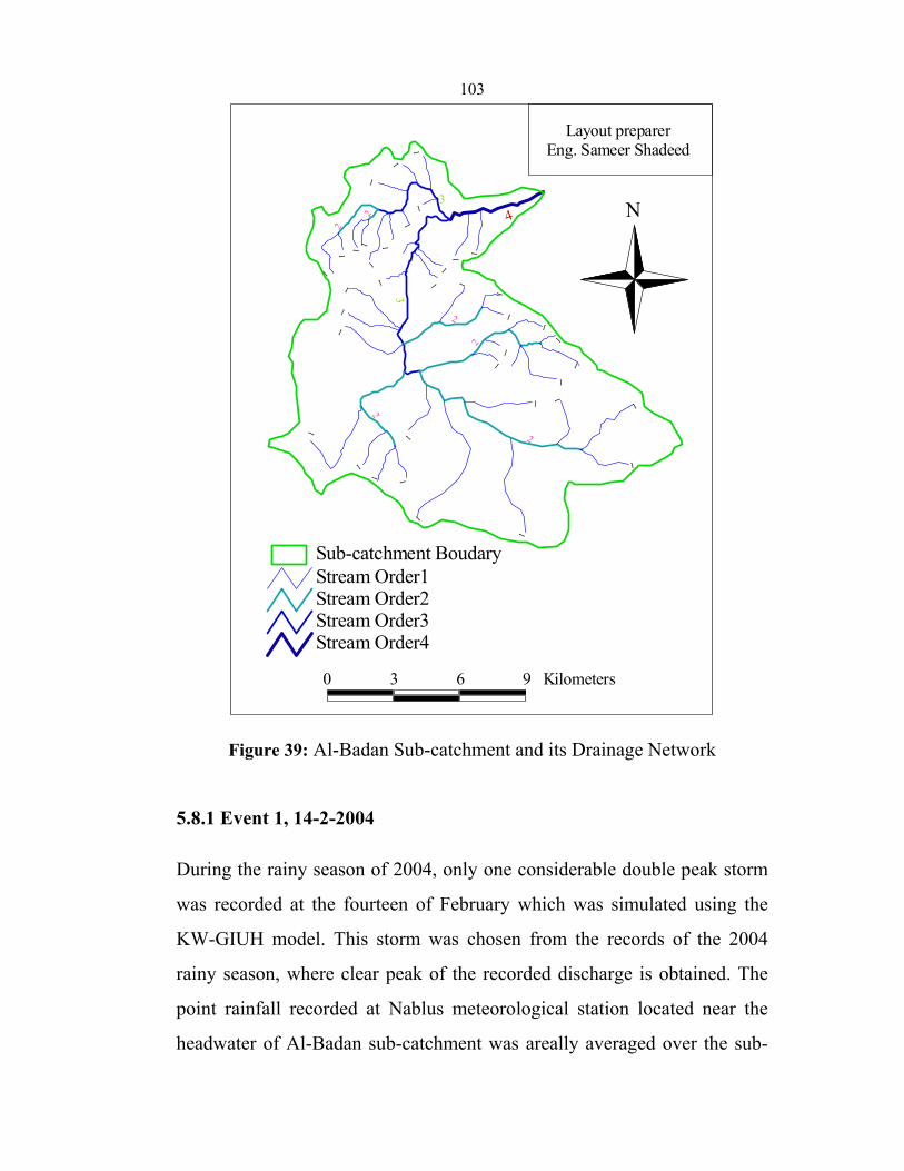
103
N
Layout preparerEng. Sameer Shadeed
0 3 6 9 Kilometers
Stream Order4Stream Order3Stream Order2Stream Order1Sub-catchment Boudary
11
1
1
1
1
1
1
1
1
1
1
1
11
1
1
1
1
1
1
1
1
1
11
1
1
1
1
1
1
1
1
1
1
11
1
4
3
3
2
2
2
2
2
2
Figure 39: Al-Badan Sub-catchment and its Drainage Network
5.8.1 Event 1, 14-2-2004
During the rainy season of 2004, only one considerable double peak storm
was recorded at the fourteen of February which was simulated using the
KW-GIUH model. This storm was chosen from the records of the 2004
rainy season, where clear peak of the recorded discharge is obtained. The
point rainfall recorded at Nablus meteorological station located near the
headwater of Al-Badan sub-catchment was areally averaged over the sub-
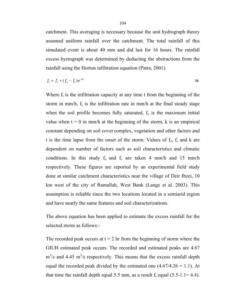
104
catchment. This averaging is necessary because the unit hydrograph theory
assumed uniform rainfall over the catchment. The total rainfall of this
simulated event is about 40 mm and did last for 16 hours. The rainfall
excess hyetograph was determined by deducting the abstractions from the
rainfall using the Horton infiltration equation (Patra, 2001).
ktcoct effff −−+= )( 34
Where ft is the infiltration capacity at any time t from the beginning of the
storm in mm/h, fc is the infiltration rate in mm/h at the final steady stage
when the soil profile becomes fully saturated, fo is the maximum initial
value when t = 0 in mm/h at the beginning of the storm, k is an empirical
constant depending on soil cover complex, vegetation and other factors and
t is the time lapse from the onset of the storm. Values of fo, fc and k are
dependent on number of factors such as soil characteristics and climatic
conditions. In this study fo and fc are taken 4 mm/h and 15 mm/h
respectively. These figures are reported by an experimental field study
done at similar catchment characteristics near the village of Deir Ibzei, 10
km west of the city of Ramallah, West Bank (Lange et al. 2003). This
assumption is reliable since the two locations located in a semiarid region
and have nearly the same features and soil characterizations.
The above equation has been applied to estimate the excess rainfall for the
selected storm as follows:-
The recorded peak occurs at t = 2 hr from the beginning of storm where the
GIUH estimated peak occurs. The recorded and estimated peaks are 4.67
m3/s and 4.45 m3/s respectively. This means that the excess rainfall depth
equal the recorded peak divided by the estimated one (4.67/4.26 = 1.1). At
that time the rainfall depth equal 5.5 mm, as a result ft equal (5.5-1.1= 4.4).
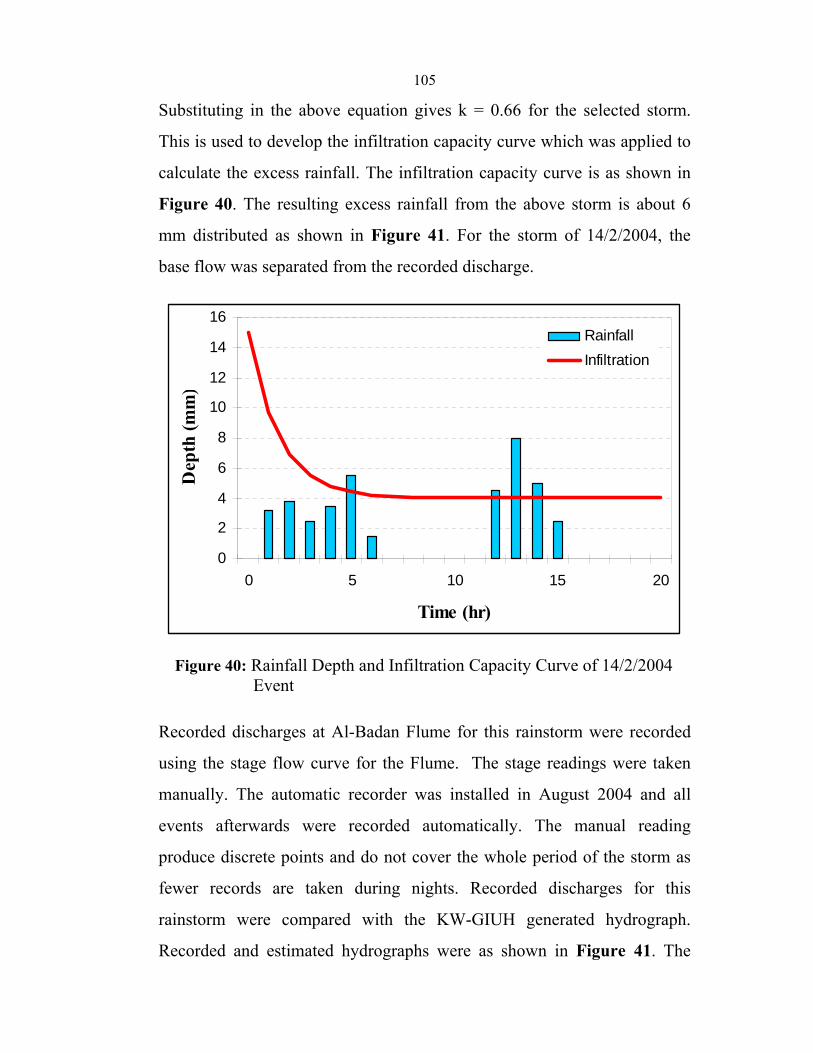
105
Substituting in the above equation gives k = 0.66 for the selected storm.
This is used to develop the infiltration capacity curve which was applied to
calculate the excess rainfall. The infiltration capacity curve is as shown in
Figure 40. The resulting excess rainfall from the above storm is about 6
mm distributed as shown in Figure 41. For the storm of 14/2/2004, the
base flow was separated from the recorded discharge.
0
2
4
6
8
10
12
14
16
0 5 10 15 20
Time (hr)
Dep
th (m
m)
RainfallInfiltration
Figure 40: Rainfall Depth and Infiltration Capacity Curve of 14/2/2004 Event
Recorded discharges at Al-Badan Flume for this rainstorm were recorded
using the stage flow curve for the Flume. The stage readings were taken
manually. The automatic recorder was installed in August 2004 and all
events afterwards were recorded automatically. The manual reading
produce discrete points and do not cover the whole period of the storm as
fewer records are taken during nights. Recorded discharges for this
rainstorm were compared with the KW-GIUH generated hydrograph.
Recorded and estimated hydrographs were as shown in Figure 41. The
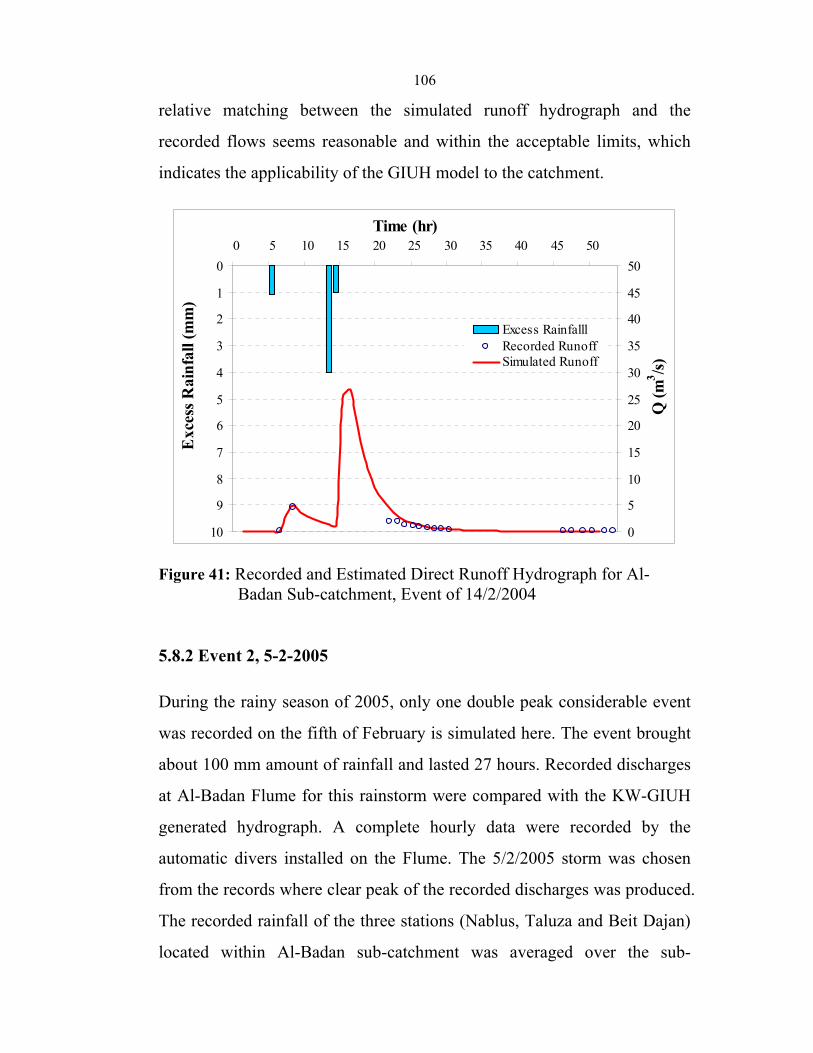
106
relative matching between the simulated runoff hydrograph and the
recorded flows seems reasonable and within the acceptable limits, which
indicates the applicability of the GIUH model to the catchment.
0
1
2
3
4
5
6
7
8
9
10
0 5 10 15 20 25 30 35 40 45 50Time (hr)
Exc
ess R
ainf
all (
mm
)
0
5
10
15
20
25
30
35
40
45
50
Q (m
3 /s)
Excess RainfalllRecorded RunoffSimulated Runoff
Figure 41: Recorded and Estimated Direct Runoff Hydrograph for Al-Badan Sub-catchment, Event of 14/2/2004
5.8.2 Event 2, 5-2-2005
During the rainy season of 2005, only one double peak considerable event
was recorded on the fifth of February is simulated here. The event brought
about 100 mm amount of rainfall and lasted 27 hours. Recorded discharges
at Al-Badan Flume for this rainstorm were compared with the KW-GIUH
generated hydrograph. A complete hourly data were recorded by the
automatic divers installed on the Flume. The 5/2/2005 storm was chosen
from the records where clear peak of the recorded discharges was produced.
The recorded rainfall of the three stations (Nablus, Taluza and Beit Dajan)
located within Al-Badan sub-catchment was averaged over the sub-
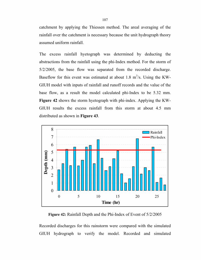
107
catchment by applying the Thiessen method. The areal averaging of the
rainfall over the catchment is necessary because the unit hydrograph theory
assumed uniform rainfall.
The excess rainfall hyetograph was determined by deducting the
abstractions from the rainfall using the phi-Index method. For the storm of
5/2/2005, the base flow was separated from the recorded discharge.
Baseflow for this event was estimated at about 1.8 m3/s. Using the KW-
GIUH model with inputs of rainfall and runoff records and the value of the
base flow, as a result the model calculated phi-Index to be 5.32 mm.
Figure 42 shows the storm hyetograph with phi-index. Applying the KW-
GIUH results the excess rainfall from this storm at about 4.5 mm
distributed as shown in Figure 43.
01
234
56
78
0 5 10 15 20 25Time (hr)
Dep
th (m
m)
RainfallPhi-Index
Figure 42: Rainfall Depth and the Phi-Index of Event of 5/2/2005
Recorded discharges for this rainstorm were compared with the simulated
GIUH hydrograph to verify the model. Recorded and simulated
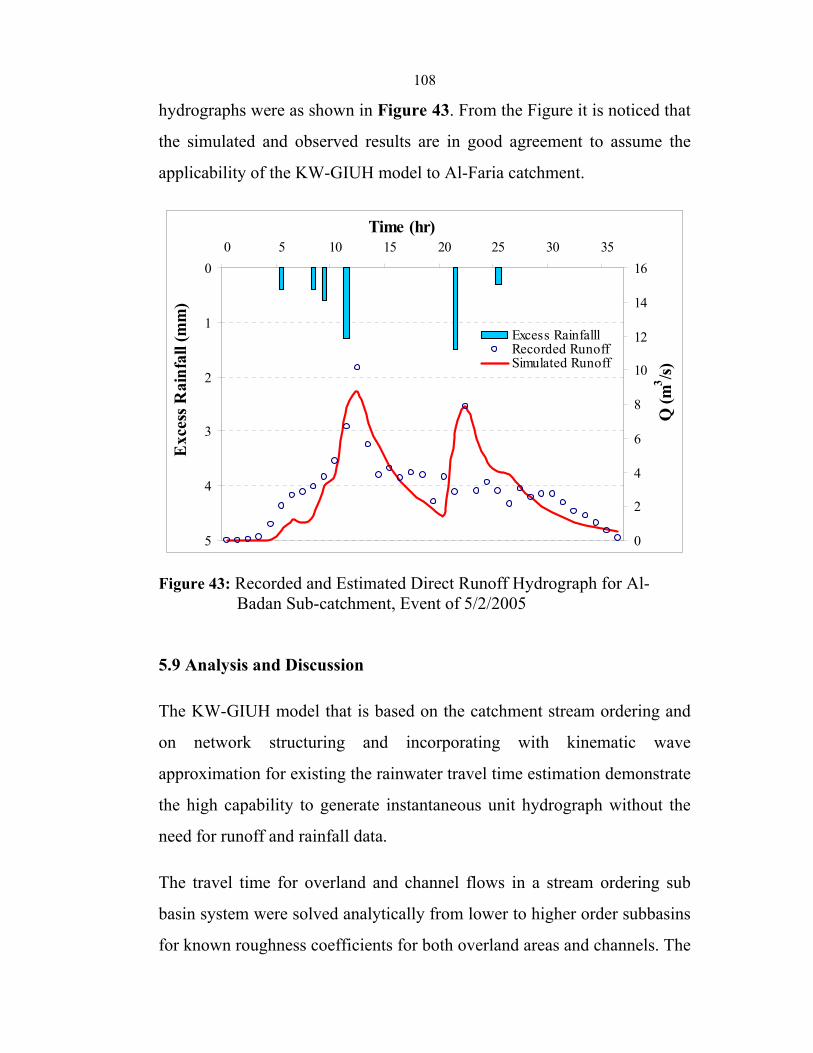
108
hydrographs were as shown in Figure 43. From the Figure it is noticed that
the simulated and observed results are in good agreement to assume the
applicability of the KW-GIUH model to Al-Faria catchment.
0
1
2
3
4
5
0 5 10 15 20 25 30 35Time (hr)
Exc
ess R
ainf
all (
mm
)
0
2
4
6
8
10
12
14
16
Q (m
3 /s)
Excess RainfalllRecorded RunoffSimulated Runoff
Figure 43: Recorded and Estimated Direct Runoff Hydrograph for Al-Badan Sub-catchment, Event of 5/2/2005
5.9 Analysis and Discussion
The KW-GIUH model that is based on the catchment stream ordering and
on network structuring and incorporating with kinematic wave
approximation for existing the rainwater travel time estimation demonstrate
the high capability to generate instantaneous unit hydrograph without the
need for runoff and rainfall data.
The travel time for overland and channel flows in a stream ordering sub
basin system were solved analytically from lower to higher order subbasins
for known roughness coefficients for both overland areas and channels. The
109
hydraulic response of a catchment was represented by the combination of a
series of probability density functions of travel time. The travel time is a
function of the amount of water in the flow that is represented by the
spatially uniform intensity of excess rainfall to be applied to the KW-GIUH
model.
In contrast to the traditional unit hydrograph theory which assumes the
linearity as one of its basic assumptions, the KW-GIUH model released this
restriction since the produced GIUH is a function of excess rainfall
considering the intensity and the interaction between surface flow and
subsurface flow intensity. Therefore, a set of GIUHs corresponding to
different values of excess rainfall can be obtained.
The critical issue in the KW-GIUH approach is the determination of excess
rainfall. In this study two methods were applied. Those are Horton equation
method and phi-index method. Results of the two methods are used to
investigate the applicability of the KW-GIUH approach to simulate the
runoff on the semiarid catchment of Faria.
Two rainstorm events were used to simulate the runoff hydrographs and to
verify the applicability of the KW-GIUH model. The first event occurred
on February 14th, 2004. The total rainfall of this event is about 40 mm
contributing to about 6 mm as excess rainfall. The resulting rainfall-runoff
ratio is about 15% for this event. The second event occurred on February
5th, 2005. This event had a total rainfall of about 100 mm and produced 4.5
mm of excess rainfall. The resulting rainfall-runoff ratio for this event is
about 4.5%. This indicates that the runoff coefficient in the catchment is in
the range of 4.5% to 15% of the annual rainfall. These results are in
110
agreement with those reported results in previous literature such as those in
(Husary et al., 1995) and (Takruri, 2003).
In this context, it is to note here that the assumption of uniform distribution
of excess rainfall over the catchment is not consistent with the semiarid
nature of the Palestinian catchments that behave as variable sources and
partially contributing. Nevertheless, the results of the simulation of the
events using the GIS-supported KW-GIUH are promising and indicate the
applicability of the model to semiarid regions.

111
CHAPTER SIX
CONCLUSIONS AND RECOMMENDATIONS
112
6.1 Conclusions
Al-Faria catchment is located in the northern West Bank, which is
characterized as semiarid. The catchment is 334 km2 and extends from the
Nablus Mountains in the west to the Jordan River in the east. The rainfall
distribution within the Faria catchment ranges from 640 mm at the
headwater to 150 mm at the outlet to the Jordan River.
Based on the analysis of the six rainfall stations in Faria catchment, it is
noticed that Nablus and Taluza stations have the largest average annual
rainfalls whereas Al-Faria station has the lowest average annual rainfall.
Tubas station has an average annual rainfall of 415 mm, which nearly
equals the arithmetic average of the annual average rainfalls of the six
stations of the catchment at about 430 mm.
From the analysis of monthly data it is clear that there is a relatively wet
period from November till April and that there is a relatively dry period
from May to October. This is associated with the climatic conditions of the
catchment.
The internal consistency of the rainfall stations of Faria catchment was
examined by using the double mass curve technique. The results proved
that all stations are internally consistent.
Significant increasing trend of rainfall averages is noticed in the case of
Nablus and Beit Dajan stations. The increasing trend of the elevated
stations and the decreasing trend of Al-Faria station, elevated below sea
level and located near the Jordan River, can be assumed in relation to the
later developments and changes in the climatic conditions of the region.
The drying of the Jordan River basin due to the diversion of the head water
113
by the Israeli projects and the Israeli National Water Carrier are assumed
among the main reasons for the observed trends. Less water is available for
evapotranspiration in the Jordan River basin and thus fewer rainfalls are
expected in contradiction to the elevated areas.
Results of probability distribution of rainfall data for the six stations has
showed that Gumbel distribution fits the annual rainfall data and can be
used for future estimations especially that the correlation coefficient, r2,
was more than 94%. This provides means to understand and evaluate the
distribution characteristics of the rainfall in the Faria catchment in
particular and of the eastern slopes of the West Bank characterized as
semiarid region in general. The obtained results are an important
contribution for the design of hydraulic projects and for the assessment of
the Palestinian water resources.
The multiple regression analysis was applied to correlate the average
annual rainfalls to the location of the stations within the catchment. The
coordinates, X and Y, and the elevations, Z, proved to be strongly
correlated to average rainfall. A statistical relation is assumed to give the
average rainfall as a function of the X, Y and Z of the station’s location.
Thiessen polygon method has been used to convert the point rainfall to
areal rainfall for the six rainfall stations. The areal average rainfall of the
Faria catchment was found at 385 mm. This value is nearly equal to the
annual average rainfall of Beit Dajan station which about 379 mm. This
indicates that the rainfall in the catchment can be represented by Beit Dajan
station.
The rainfall runoff process in the Faria catchment was investigated and
modeled. The GIUH model is the model selected for modeling the process
114
as it can be applied incorporating the geomorphological characteristics of
the catchment and with less need to highly sophisticated measurements.
The KW-GIUH hydrological model supported by the GIS is applied to
investigate the rainfall runoff process in the Faria catchment as a case study
towards understanding the storm water drainage and rainfall runoff process
in the West Bank.
GIUH unit hydrographs were derive for the three sub-catchments of the
whole Faria catchment. These sub-catchments are Al-Badan, Al-Faria and
Al-Malaqi having areas of about 85 km2, 64 km2 and 185 km2 respectively.
Estimated peak discharges of 1-mm excess rainfall for three sub-
catchments are 4.26 m3/s, 3.21 m3/s and 7.4 m3/s respectively.
Two rainfall events were simulated on Al-Badan sub-catchment using the
generated KW-GIUH hydrograph. Estimated hydrographs were compared
with the recorded discharges to verify the results of the model and
reasonable matching was obtained. From the obtained results, it can be
concluded that the runoff in the Faria catchment is in the range of 4.5% to
15% of the annual rainfall.
6.2 Recommendations
Based on the findings of this work, the following points can be
recommended for future research in the field of surface water hydrology in
Palestine and in semiarid regions.
1. Use the results of Faria catchment and translate it towards
understanding and managing the water resources in Jordan
Valley.

115
2. Flow measuring devices were built at the outlet of Al-Badan and
Al-Faria sub-catchments in the context of GLOWA JR project
should be maintained to remain working properly. Yearly
maintenance is recommended for these stations to insure the
quality of obtained data, and thus enhance the evaluation of the
applicability of the developed GIUH model.
3. It is recommended to install automatic instruments for measuring
other hydrological parameters. These include rainfall intensity,
runoff and infiltration in addition to detailed measurement of all
meteorological parameters such as evaporation, temperature,
humidity, wind speed and others.
4. Available roughness coefficient data is minimal. More extensive
data is needed so that assumption concerning this parameter in
the model is more realistic.
5. More rainstorm events are required to be investigated in order to
calibrate and verify the applicability of the developed GIUH
model.
6. The GIUH model should be applied to other catchments in
Palestine to evaluate the applicability and reliability of this model
and to investigate rainfall runoff process in Palestine representing
a semiarid region.
7. Develop the available GIS system in the Palestinian Authorities
use it to develop catchment characteristics. These data should be
made available to researches for further applications. The GIS

116
system and data can then be convolved to the GIUH program and
other available models.
8. Constructing a dam at Jiser Al-Malaqi to store winter floodwaters
will serve the long term objectives of water resources
management of Faria catchment.
117
References
Abrahams, A. D., Parsons, A. J. and Wainwright, J. (1994). Resistance to
overland flow on semiarid grassland and shrubland hillslopes,
Walnut Gulch, southern Arizona. Journal of Hydrology. Vol. 156, P.
431-46.
Agnese, C. D., Asaro, D. and Giordano, G. (1988). Estimation of the time
scale of the geomorphologic instantaneous unit hydrograph from
effective streamflow velocity. Water Resource. Vol. 24, No. 7, P.
969-978.
Al-Nubani, N. I. (2000). Rainfall – Runoff Process and Rainfall Analysis
for Nablus Basin. M.Sc. Thesis, Faculty of Graduate Studies, An-
Najah National University, Nablus, Palestine.
Al-Smadi, M. (1998). Incorporating Spatial and Temporal Variation of
Watershed Response in a GIS-Based Hydrologic Model. M.Sc.
Thesis, Biological Systems Engineering Department. Virginia Tech,
Blcksburg.
Andrew N. S. and Patrick. A. O. (2004). Stormwater Master Planning with
GIS, A Case Study of the Blue River Watershed.
Applied Research Institute-Jerusalem (ARIJ). (1996). Environmental
Profile for the West Bank, Volume 5, Nablus Profile. Palestine.
Caritas Street, Bethlehem.
Barakat, M. H. (2000). Rainfall – Runoff Process and Modeling for Soreq
stream near Jerusalem. M.Sc. Thesis, Faculty of Graduate Studies,
An-Najah National University, Nablus, Palestine.
Barkhordari, J. (2003). Assessing the Effects of Land use Change on the
Hydrologic Regime by RS and GIS. A case Study in the Minab
118
Catchment. M.Sc. Thesis, International Institute for Geo-
information Science and Earth Observation, Hormozgan province,
Iran.
Bergström, S., Forsman, A. (1973). Development of A conceptual
Deterministic Rainfall Runoff Model. Nordic Hydrology, Vol. 4, P.
147-170.
Berod, D.D., Singh, V.P. and Musy, A. (1999). A geomorphologic
kinematic-wave (GKW) model for estimation of floods from small
alpine watersheds. Hydrological Process. Vol. 13, P. 1391-1416.
Beven, K. J and Kirkby, M. J. (1979). A physically Based Variable
Contributing Area Model of Basin Hydrology. Hydrological Science
Bulletin, Vol. 24, No. 1, P. 43-69.
Bhaskar, N. R., James, W. P., and Devulapall, R. S. (1992). Hydrologic
Parameter Estimation Using Geographic Information System.
Journal of Water Resources Planning and Management, Vol. 118,
No. 5, P. 492-512.
Brooks, S.M., McDonnell, R.A., 2000. Research advances geocomputation
for hydrological and geomorphological modeling towards the
twenty-first century. Hydrological Process. Vol. 14, P. 1899-1907.
Crawford, N.H and Linsley, R.K. (1966). Digital Simulation in Hydrology,
Stanford Watershed Model. Technical Report No. 39, Civil
Engineering Department, Stanford University.
Chow, V.T, Maidment, David R and Mays, L.W. (1988). Applied
Hydrology. McGRAW-HILL, New York.
119
Chutha, P. and Dooge, J.C.I. (1990). The shape parameters of the
geomorphologic unit hydrograph. Journal of Hydrology. Vol. 117, P.
81-97.
Chow, V.T. (1964). Handbook of Applied Hydrology, A Compendium of
Water Resources Technology, Mc-Graw Hill book Company, New
York.
EQA. (2004). Al-Faria – Jerash Integrated Watershed Management Project
(WASMAP), Wadi Al-Faria Baseline Report. Unpublished Report.
FAO (1989). Arid Zone Forestry, A guide for Field Technicians.
Ghanem, M. (1999). Hydrology and Hydrochemistry of the Faria Drainage
Basin / West Bank. Ph.D. Thesis, Wissenschaftliche Mitteilungen,
Institut Fur Geologie, Technische Universital Bergakademie
Freiburg, Germany.
Graf, W. L. (1988). Fluvial Processes in Dryland Rivers. Springer Series in
Physical Environment. Springer, Heidelberg.
Grover, S. (2003). Perspectives of GIS Modeling in Hydrology. Natural
Resources Management, GIS Development.
Gupta, V.K., Waymire, E. and Wang, C.T. (1980). A representation of an
Instantaneous Unit hydrograph From Geomorphology. Water
Resources Research, Vol. 16, No. 5, P. 855-862.
Haan, C.T. (1977). Statistical Methods in Hydrology. The Iowa State
University Press, Ames, USA.
Hall, M.J., Zaki, A.F. and Shahin, M.A. (2001). Regional Analysis Using
the Geomorphoclimatic Instantaneous Unit Hydrograph. Hydrology
and Earth System Sciences, Vol. 5, No. 1, P. 93–102.
120
Hussary, Samar; Najjar, Tagreed; and Aliewi, Amjad. (1995). Analysis of
Secondary Source Rainfall Data from the Northern West Bank.
Palestinian Hydrology Group and University of New Castle upon
type, Jerusalem ,West Bank ,Palestine.
Jain, S.K., Singh, R.D., and Seth, S.M. (2000). Design Flood Estimation
Using GIS Supported GIUH Approach, Water Resources
Management, Vol. 14, P. 369-376.
Jin, C. (1992). A deterministic gamma-type geomorphological
instantaneous unit hydrograph based on path types. Water Resources.
Vol. 28, No. 2, P. 479-486.
Karlinger, M.R. and Troutman, B.M. (1985). Assessment of the
instantaneous unit hydrograph derived from the theory of
topologically random networks. Water Resource. Vol. 21, No, 11,
P.1693–1702.
Kirshen, D.M. and Bras, R.L. (1983). The linear channel and its effect on
the geomorphologic IUH. Journal of Hydrology. Vol. 65, P.175–208.
Lange, J. (1999). A noncalibrated Rainfall-Runoff Model for Large, Arid
Catchments, Nahal Zin, Israel. PhD Thesis, Freiburg University,
Institute of Hydrology.
Lange, J and Leibundgut, C. Greenbaum, N and Schick, A.P (1999). A
noncalibrated Rainfall-Runoff Model for Large, Arid Catchments,
Institute of Hydrology, University of Freiburg, Freiburg, Germany
and Department of Geography, Hebrew University. Water
Resources Research, Vol. 35, No. 7, P. 2161–2172.
Lange, J., Greenbaum, N., Husary, S., Ghanem, M., Leibundgut, C. and
Schick, A. (2003). Runoff Generation from Successive Simulated
121
Rainfalls on A rocky, Semi-arid, Mediterranean Hillslope. Hydrol.
Process. Vol. 17, P. 279–296.
Lee, K.T., and Chang, C.H. (2005). Incorporating Subsurface Flow
Mechanism into Geomorphology-Based IUH Modeling. Department
of River and Harbor Engineering, National Taiwan Ocean
University, 2, Bee-Ning Road, Keelung, Taiwan 202, ROC.
Lim, C. K. (2003). Applying GIS to Hydraulic Analysis. Department of
Civil Engineering, Texas University.
Linsly, R.K., Kahler, M.A and Paullus, J.L. (1982). Hydrology for
Engineers. Third Edition. McGraw-Hill International Book
Company.
Lundin, L.C., Sten Bergström, S., Eriksson, E. and Seibert, J. (1998).
Hydrological Models and Modeling.
Maidment, D.R. (1996). GIS and Hydrologic Modeling. An Assessment of
Progress, Presented at the Third International Conference on GIS
and Environmental Modeling, Santa Fe, New Mexico, 22-26.
Maffini, G. (1997). Using GIS Technology to Advance and Optimize Asset
Management. Presentation to Strategic and Profitable Asset
Management Conference, London.
MOT. (1998). Palestine Climatic Data Handbook. Metrological Office,
Ministry of Transport, Palestinian National Authority.
Nash, J.E. (1958). The Form of the Instantaneous Unit Hydrograph. IAHS-
Publ. No. 45, P. 114-121.
122
Orthor, R., Loibl, W. and Wenl, E. (2001). A Harmonized Water Data Base
for the Lower Jordan Valley. ARC Seibersdorf Research Report
ARC.S-0157, Ein Untemehment der Austrian Research Centers.
Patra, K.C. (2001). Hydrology and Water Resources Engineering. Alpha
Science International Ltd. India.
Petts, G.E. (1995). Changing River Channels. The Geographical Tradition.
John Wiley & Sons, Chichester, P. 1-23.
Ponce, V.M. (1989). Engineering Hydrology, Principles and Practices.
Prenctice Hall, Englewood Cliffs, New Jersey, USA.
Raghunath H.M. (1985). Hydrology, Principles, Analysis, Design. New
Age International Publishers.
Rodriguez-Iturbe, I. and Valdes, J.B. (1979). The Geomorphological
Structure of Hydrologic Response. Gradate Program in Hydrology
and Water Resources, Universidad Simon Bolivar, Caracas,
Venezuela.
Rodriguez-Iturbe, I., Gonzalez-Sanabria, M. and Bras, R.L. (1982). A
geomorphoclimatic theory of the instantaneous unit hydrograph.
Water Resource. Vol. 18, No. 4, P. 877-886.
Rofe and Rafety Consulting Engineering. (1965). West Bank Hydrology,
Analysis 1963-1965, Geological and Hydrological Report,
Hashimite Kingdom of Jordan, Central Water Authority, Jordan.
Schick, A.P., Grodek, T. and Lekach, J. (1997). Sediment Management and
Flood Protection of Desert Towns: Effects of Small Catchments.
Human Impact on Erosion and Sedimentation. IAHS- Wallingford,
No. 245.
123
Shadeed, S.M. and Wahsh, H.F. (2002). Synthetic Modeling of Rainfall-
Runoff Process of upper Faria Catchment. B.Sc. thesis, Faculty of
Civil Engineering An-Najah National University, Nablus, Palestine.
Shaheen, H.Q. (2002). Storm Water Drainage in Arid and Semiarid
Regions: West Bank as A case Study, An-Najah University Journal
for Research - Natural Sciences, Vol. 16, No. 12, P. 125-137.
Sherman, L.K. (1932). Stream flow from Rainfall by Unit Hydrograph
Method, Engineering News Records, V. 108, P.501-505.
Snell, J.D. and Sivapalan, M. (1994). On Geomorphological Dispersion in
Natural Catchments and the Geomorphological Unit Hydrograph,
Water Resources Research, Vol. 30, No. 7, P. 2311-2323.
Sorman, A.U. (1995). Estimation of Peak Discharge Using GIUH Model in
Saudi Arabia. Journal of Water Resources Planning and
Management, Vol. 121, No. 4, P. 287-293.
Strahler, A.N. (1957). Quantitative Analysis of Watershed Geomorphology,
Transactions, American Geographical Union.
Takruri, B.B. (2003). Rainfall-Runoff Analysis and the Synthetic Unit
Hydrograph for Wadi Faria Catchment. M.Sc. Thesis, Faculty of
Graduate Studies, Beir Zeit University, Palestine
Todini, E. (1988). Rainfall Runoff Modeling-Past, Present and Future.
Journal of Hydrology, Vol. 100, P 341-352.
Thormählen, A.C. (2003). Hydrological Modeling in A small Hyperarid
Catchment. Nahal Yael, Israel. M.Sc. Thesis, Institute of Hydrology,
Freiburg University, Germany.
124
UNESCO. (1984). Map of the world Distribution of Arid Regions. Paris,
France.
Viessman, W.J., Lewis, G.L. and Knapp J.W. (2003). Introduction to
Hydrology. Fifth Edition, Harper Collins.
Wilson, E.M. (1974). Engineering Hydrology, Second Edition, The
Macmillan Press ltd., London Basingstoke Companies.
Yen, B.C., and Lee, K.T. (1997). Unit Hydrograph Derivation for
Ungauged Watersheds by Stream-Order Laws, Journal of
Hydrologic Engineering, ASCE, Vol. 2, No. 1, P. 1-9.

125Appendix A (Tables)
Table A1 1: Monthly Climatic Average Data of Al-Farai Station ................. 127 Table A1 2: Monthly Climatic Average Data of Nablus Station. ................. 128 Table A2 1: CROPWAT 4 Output Results for Nablus Station ...................... 130 Table A2 2: CROPWAT 4 Output Results for Al-Faria Station .................... 130 Table A3 1: Basic Information of Wells Located within the Faria Catchment ..... 132 Table A4 1: Monthly Flow Discharge of Shibli Spring ................................. 137 Table A4 2: Monthly Flow Discharge of Faria Spring .................................. 138 Table A4 3: Monthly Flow Discharge of Miska Spring ................................. 139 Table A4 4: Monthly Flow Discharge of Dafna Spring ................................. 140 Table A4 5: Monthly Flow Discharge of Balata Spring ................................ 141 Table A4 6: Monthly Flow Discharge of Asubian Spring ............................. 142 Table A4 7: Monthly Flow Discharge of Duleib Spring ................................ 143 Table A4 8: Monthly Flow Discharge of Qudeira Spring .............................. 144 Table A4 9: Monthly Flow Discharge of Hamad & Beida Spring ................. 145 Table A4 10: Monthly Flow Discharge of Al-Jiser Spring ............................ 146 Table A4 11: Monthly Flow Discharge of Sidreh Spring .............................. 147 Table A4 12: Monthly Flow Discharge of Tabban Spring ............................. 148 Table A4 13: Monthly Flow Discharge of Abu Saleh Spring ........................ 149 Table A5 1: Flow Records of Al-Badan and Al-Faria Flumes ....................... 151 Table A6 1: Annual Rainfall Data of the Faria Catchment Stations .............. 160

126
APPENDIX A1
MONTHLY CLIMATIC AVERAGES DATA
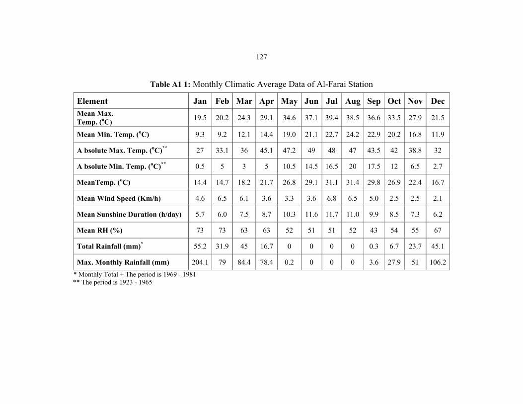
127
Table A1 1: Monthly Climatic Average Data of Al-Farai Station
Element Jan Feb Mar Apr May Jun Jul Aug Sep Oct Nov Dec Mean Max. Temp. (oC) 19.5 20.2 24.3 29.1 34.6 37.1 39.4 38.5 36.6 33.5 27.9 21.5
Mean Min. Temp. (oC) 9.3 9.2 12.1 14.4 19.0 21.1 22.7 24.2 22.9 20.2 16.8 11.9
A bsolute Max. Temp. (oC)** 27 33.1 36 45.1 47.2 49 48 47 43.5 42 38.8 32
A bsolute Min. Temp. (oC)** 0.5 5 3 5 10.5 14.5 16.5 20 17.5 12 6.5 2.7
MeanTemp. (oC) 14.4 14.7 18.2 21.7 26.8 29.1 31.1 31.4 29.8 26.9 22.4 16.7
Mean Wind Speed (Km/h) 4.6 6.5 6.1 3.6 3.3 3.6 6.8 6.5 5.0 2.5 2.5 2.1
Mean Sunshine Duration (h/day) 5.7 6.0 7.5 8.7 10.3 11.6 11.7 11.0 9.9 8.5 7.3 6.2
Mean RH (%) 73 73 63 63 52 51 51 52 43 54 55 67
Total Rainfall (mm)* 55.2 31.9 45 16.7 0 0 0 0 0.3 6.7 23.7 45.1
Max. Monthly Rainfall (mm) 204.1 79 84.4 78.4 0.2 0 0 0 3.6 27.9 51 106.2 * Monthly Total + The period is 1969 - 1981 ** The period is 1923 - 1965

128
Table A1 2: Monthly Climatic Average Data of Nablus Station Element Jan Feb Mar Apr May Jun Jul Aug sep Oct Nov Dec
Mean Max. Temp. (oC) 13.1 14.4 17.2 22.2 25.7 27.9 29.1 29.4 28.4 25.8 20.2 14.6
Mean Min. Temp. (oC) 6.2 6.7 8.8 12.1 14.9 17.4 19.3 19.5 18.5 16.2 12.1 7.8
A bsolute Max. Temp. (oC) 22.9 28.1 30.4 35 38.6 38 38.1 38.6 38.8 35.3 30.7 28
A bsolute Min. Temp. (oC) -0.6 -2.8 -1 0.6 6.9 11.4 12.3 15.9 13 9.3 1.4 0.3
MeanTemp. (oC) 9.6 10.5 13 17.1 20.3 22.6 24.2 24.4 23.4 21 16.1 11.2
Mean Wind Speed (Km/h) 8.7 9.5 10 10.2 10.7 12 12.4 11.7 10.3 7.7 7.8 7.7
Pressure (mbar) 953 952 951 949 948 946 944 945 948 951 953 953
Mean Sunshine Duration (h/day) 4.7 4.8 6.4 8.2 8.9 8.4 9.6 10.9 10.2 9.8 7 4.5
Mean RH (%) 67 67 62 53 51 55 61 65 64 57 57 67
Total Rainfall (mm)* 141.1 146.9 104 20.2 7.8 0 0 0 1.8 20.7 77.1 140.5
Total Evaporation (mm)* 49 67 99 149 203 226 238 218 178 131 75 49
Total PET (mm)* 36 36 55 82 106 112 117 112 105 103 72 36
Max. Monthly Rainfall (mm) 389 389 220 225 65 3 0 1 22 83 249 472 * Monthly Total
129
APPENDIX A2
CROPWAT 4 OUTPUT RESULTS FOR NABLUS AND AL-FARIA STATIONS
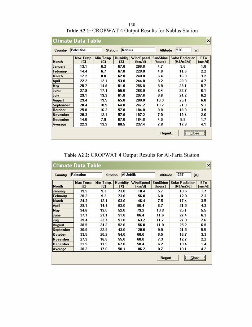
130Table A2 1: CROPWAT 4 Output Results for Nablus Station
Table A2 2: CROPWAT 4 Output Results for Al-Faria Station
131
APPENDIX A3
GROUNDWATER WELLS IN THE FARIA CATCHMENT
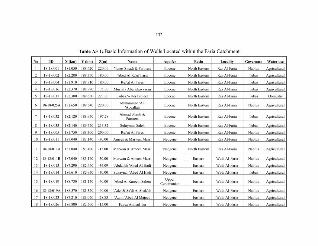
132
Table A3 1: Basic Information of Wells Located within the Faria Catchment
No ID X (km) Y (km) Z(m) Name Aquifer Basin Locality Governate Water use
1 18-18/001 181.050 188.620 220.00 Yunes Swadi & Partners Eocene North Eastern Ras Al-Faria Nablus Agricultural
2 18-18/002 182.200 188.350 180.00 'Abed Al Ra'uf Faris Eocene North Eastern Ras Al-Faria Tubas Agricultural
3 18-18/004 181.910 188.710 180.00 Ref'at Al Fares Eocene North Eastern Ras Al-Faria Tubas Agricultural
4 18-18/016 182.370 188.890 175.00 Mustafa Abu Khayzaran Eocene North Eastern Ras Al-Faria Tubas Agricultural
5 18-18/017 182.300 189.650 223.00 Tubas Water Project Eocene North Eastern Ras Al-Faria Tubas Domestic
6 18-18/025A 181.650 189.540 220.00 Muhammad 'Ali 'Abdallah Eocene North Eastern Ras Al-Faria Nablus Agricultural
7 18-18/032 182.120 188.950 197.28 Ahmad Shanti & Partners Eocene North Eastern Ras Al-Faria Tubas Agricultural
8 18-18/033 182.140 189.770 213.32 Sulayman Saleh Eocene North Eastern Ras Al-Faria Tubas Agricultural
9 18-18/005 181.750 188.300 200.00 Ref'at Al Fares Eocene North Eastern Ras Al-Faria Nablus Agricultural
10 18-18/011 187.040 183.140 -30.00 Ameen & Marwan Masri Neogene North Eastern Ras Al-Faria Nablus Agricultural
11 18-18/011A 187.040 183.400 -15.00 Marwan & Ameen Masri Neogene North Eastern Ras Al-Faria Nablus Agricultural
12 18-18/011B 187.040 183.140 -30.00 Marwan & Ameen Masri Neogene Eastern Wadi Al-Faria Nablus Agricultural
13 18-18/013 187.290 182.440 -36.09 'Abdallah 'Abed Al Hadi Neogene Eastern Wadi Al-Faria Nablus Agricultural
14 18-18/014 186.610 182.950 -30.00 Sukaynah 'Abed Al Hadi Neogene Eastern Wadi Al-Faria Tubas Agricultural
15 18-18/019 188.730 181.150 -40.00 'Abed Al Kareem Salem Upper Cenomanian Eastern Wadi Al-Faria Nablus Agricultural
16 18-18/019A 188.570 181.320 -40.00 'Adel & Sa'di Al Shak'ah Neogene Eastern Wadi Al-Faria Nablus Agricultural
17 18-18/023 187.210 183.070 -28.83 'Azmi 'Abed Al Majeed Neogene Eastern Wadi Al-Faria Nablus Agricultural
18 18-18/026 186.800 182.500 -15.00 Fayez Ahmad 'Isa Neogene Eastern Wadi Al-Faria Nablus Agricultural
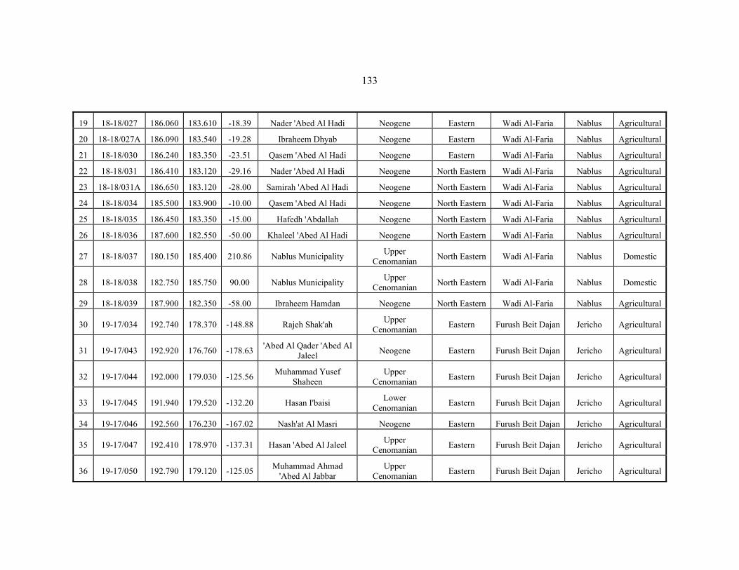
133
19 18-18/027 186.060 183.610 -18.39 Nader 'Abed Al Hadi Neogene Eastern Wadi Al-Faria Nablus Agricultural
20 18-18/027A 186.090 183.540 -19.28 Ibraheem Dhyab Neogene Eastern Wadi Al-Faria Nablus Agricultural
21 18-18/030 186.240 183.350 -23.51 Qasem 'Abed Al Hadi Neogene Eastern Wadi Al-Faria Nablus Agricultural
22 18-18/031 186.410 183.120 -29.16 Nader 'Abed Al Hadi Neogene North Eastern Wadi Al-Faria Nablus Agricultural
23 18-18/031A 186.650 183.120 -28.00 Samirah 'Abed Al Hadi Neogene North Eastern Wadi Al-Faria Nablus Agricultural
24 18-18/034 185.500 183.900 -10.00 Qasem 'Abed Al Hadi Neogene North Eastern Wadi Al-Faria Nablus Agricultural
25 18-18/035 186.450 183.350 -15.00 Hafedh 'Abdallah Neogene North Eastern Wadi Al-Faria Nablus Agricultural
26 18-18/036 187.600 182.550 -50.00 Khaleel 'Abed Al Hadi Neogene North Eastern Wadi Al-Faria Nablus Agricultural
27 18-18/037 180.150 185.400 210.86 Nablus Municipality Upper Cenomanian North Eastern Wadi Al-Faria Nablus Domestic
28 18-18/038 182.750 185.750 90.00 Nablus Municipality Upper Cenomanian North Eastern Wadi Al-Faria Nablus Domestic
29 18-18/039 187.900 182.350 -58.00 Ibraheem Hamdan Neogene North Eastern Wadi Al-Faria Nablus Agricultural
30 19-17/034 192.740 178.370 -148.88 Rajeh Shak'ah Upper Cenomanian Eastern Furush Beit Dajan Jericho Agricultural
31 19-17/043 192.920 176.760 -178.63 'Abed Al Qader 'Abed Al Jaleel Neogene Eastern Furush Beit Dajan Jericho Agricultural
32 19-17/044 192.000 179.030 -125.56 Muhammad Yusef Shaheen
Upper Cenomanian Eastern Furush Beit Dajan Jericho Agricultural
33 19-17/045 191.940 179.520 -132.20 Hasan I'baisi Lower Cenomanian Eastern Furush Beit Dajan Jericho Agricultural
34 19-17/046 192.560 176.230 -167.02 Nash'at Al Masri Neogene Eastern Furush Beit Dajan Jericho Agricultural
35 19-17/047 192.410 178.970 -137.31 Hasan 'Abed Al Jaleel Upper Cenomanian Eastern Furush Beit Dajan Jericho Agricultural
36 19-17/050 192.790 179.120 -125.05 Muhammad Ahmad 'Abed Al Jabbar
Upper Cenomanian Eastern Furush Beit Dajan Jericho Agricultural

134
37 19-17/051 192.170 179.300 -127.49 Tawfeeq Yazdi Upper Cenomanian Eastern Furush Beit Dajan Jericho Agricultural
38 19-17/057 192.180 179.000 -135.00 'Atara -Mekorot No.1 Upper Cenomanian Eastern Furush Beit Dajan Jericho Israeli
39 19-17/058 193.370 176.660 -160.00 Masawa No. 1 Lower+Upper Eastern Furush Beit Dajan Jericho Israeli
40 19-17/059 191.560 173.370 19.21 Geteet No.3 Lower Cenomanian Eastern Furush Beit Dajan Jericho Israeli
41 19-17/060 189.980 178.240 50.00 'Atara No.2 Lower Cenomanian Eastern Furush Beit Dajan Jericho Israeli
42 19-16/001 196.770 169.900 -260.00 'Ali 'Abdallah Damen Alluvium Eastern Al Jiftlik Jericho Agricultural
43 19-16/003 198.460 169.650 -280.00 Ahmad Hashem Al Zghayyer Alluvium Eastern Al Jiftlik Jericho Agricultural
44 19-16/004 198.200 169.300 -273.00 Ahmad Hashem Al Zghayyer Alluvium Eastern Al Jiftlik Jericho Agricultural
45 19-16/005 199.590 168.850 -290.00 'Abed Al'azeez Lubbad Sarrees Alluvium Eastern Al Jiftlik Jericho Agricultural
46 19-16/008 196.780 169.670 -260.00 Burhan Damen Alluvium Eastern Al Jiftlik Jericho Agricultural
47 19-16/009 196.970 169.220 -265.00 Nawwaf Al Damen Alluvium Eastern Al Jiftlik Jericho Agricultural
48 19-16/010 196.850 169.730 -260.00 Shaher Al Damen Alluvium Eastern Al Jiftlik Jericho Agricultural
49 19-17/001 196.900 170.740 -255.00 'Inad Al Masri Alluvium Eastern Al Jiftlik Jericho Agricultural
50 19-17/002 196.520 171.240 -252.60 Waheed Al Masri Eocene Eastern Al Jiftlik Jericho Agricultural
51 19-17/004 197.220 170.560 -260.00 Al Jiftlik Nursery No. 3 Alluvium Eastern Al Jiftlik Jericho Agricultural
52 19-17/005 197.220 170.560 -260.00 Al Jiftlik Nursery No.5 Alluvium Eastern Al Jiftlik Jericho Agricultural
53 19-17/006 196.780 170.000 -260.00 Adham Al Damen Alluvium Eastern Al Jiftlik Jericho Agricultural
54 19-17/007 196.640 172.290 -243.65 Fathalla Al Masri Eocene Eastern Al Jiftlik Jericho Agricultural
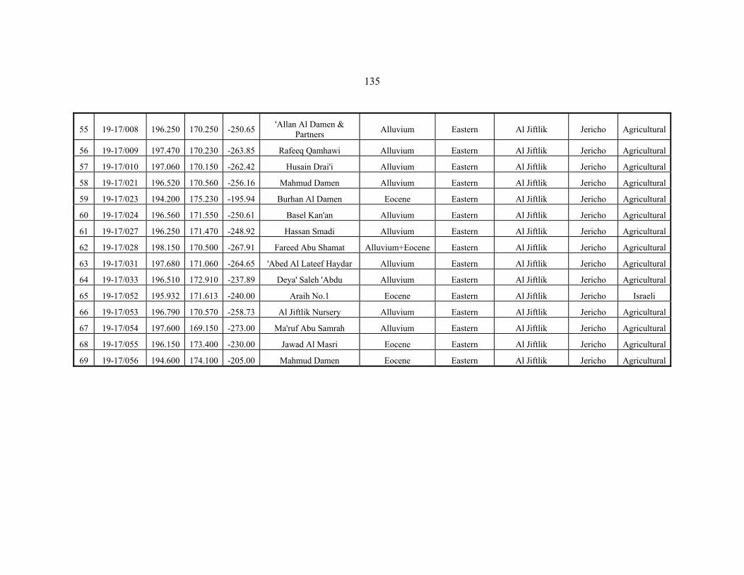
135
55 19-17/008 196.250 170.250 -250.65 'Allan Al Damen & Partners Alluvium Eastern Al Jiftlik Jericho Agricultural
56 19-17/009 197.470 170.230 -263.85 Rafeeq Qamhawi Alluvium Eastern Al Jiftlik Jericho Agricultural
57 19-17/010 197.060 170.150 -262.42 Husain Drai'i Alluvium Eastern Al Jiftlik Jericho Agricultural
58 19-17/021 196.520 170.560 -256.16 Mahmud Damen Alluvium Eastern Al Jiftlik Jericho Agricultural
59 19-17/023 194.200 175.230 -195.94 Burhan Al Damen Eocene Eastern Al Jiftlik Jericho Agricultural
60 19-17/024 196.560 171.550 -250.61 Basel Kan'an Alluvium Eastern Al Jiftlik Jericho Agricultural
61 19-17/027 196.250 171.470 -248.92 Hassan Smadi Alluvium Eastern Al Jiftlik Jericho Agricultural
62 19-17/028 198.150 170.500 -267.91 Fareed Abu Shamat Alluvium+Eocene Eastern Al Jiftlik Jericho Agricultural
63 19-17/031 197.680 171.060 -264.65 'Abed Al Lateef Haydar Alluvium Eastern Al Jiftlik Jericho Agricultural
64 19-17/033 196.510 172.910 -237.89 Deya' Saleh 'Abdu Alluvium Eastern Al Jiftlik Jericho Agricultural
65 19-17/052 195.932 171.613 -240.00 Araih No.1 Eocene Eastern Al Jiftlik Jericho Israeli
66 19-17/053 196.790 170.570 -258.73 Al Jiftlik Nursery Alluvium Eastern Al Jiftlik Jericho Agricultural
67 19-17/054 197.600 169.150 -273.00 Ma'ruf Abu Samrah Alluvium Eastern Al Jiftlik Jericho Agricultural
68 19-17/055 196.150 173.400 -230.00 Jawad Al Masri Eocene Eastern Al Jiftlik Jericho Agricultural
69 19-17/056 194.600 174.100 -205.00 Mahmud Damen Eocene Eastern Al Jiftlik Jericho Agricultural
136
Appendix A4
Monthly Flow Discharge of the Springs in the Faria Catchment
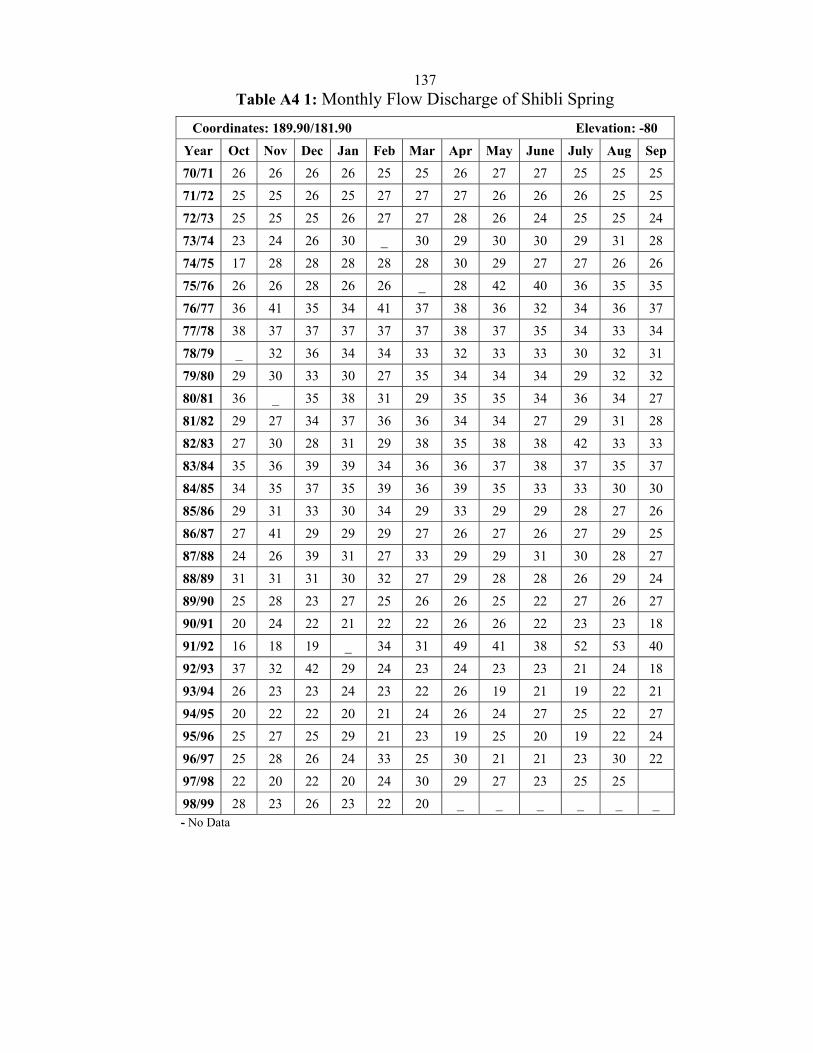
137Table A4 1: Monthly Flow Discharge of Shibli Spring
Coordinates: 189.90/181.90 Elevation: -80
Year Oct Nov Dec Jan Feb Mar Apr May June July Aug Sep 70/71 26 26 26 26 25 25 26 27 27 25 25 25
71/72 25 25 26 25 27 27 27 26 26 26 25 25
72/73 25 25 25 26 27 27 28 26 24 25 25 24
73/74 23 24 26 30 _ 30 29 30 30 29 31 28
74/75 17 28 28 28 28 28 30 29 27 27 26 26
75/76 26 26 28 26 26 _ 28 42 40 36 35 35
76/77 36 41 35 34 41 37 38 36 32 34 36 37
77/78 38 37 37 37 37 37 38 37 35 34 33 34
78/79 _ 32 36 34 34 33 32 33 33 30 32 31
79/80 29 30 33 30 27 35 34 34 34 29 32 32
80/81 36 _ 35 38 31 29 35 35 34 36 34 27
81/82 29 27 34 37 36 36 34 34 27 29 31 28
82/83 27 30 28 31 29 38 35 38 38 42 33 33
83/84 35 36 39 39 34 36 36 37 38 37 35 37
84/85 34 35 37 35 39 36 39 35 33 33 30 30
85/86 29 31 33 30 34 29 33 29 29 28 27 26
86/87 27 41 29 29 29 27 26 27 26 27 29 25
87/88 24 26 39 31 27 33 29 29 31 30 28 27
88/89 31 31 31 30 32 27 29 28 28 26 29 24
89/90 25 28 23 27 25 26 26 25 22 27 26 27
90/91 20 24 22 21 22 22 26 26 22 23 23 18
91/92 16 18 19 _ 34 31 49 41 38 52 53 40
92/93 37 32 42 29 24 23 24 23 23 21 24 18
93/94 26 23 23 24 23 22 26 19 21 19 22 21
94/95 20 22 22 20 21 24 26 24 27 25 22 27
95/96 25 27 25 29 21 23 19 25 20 19 22 24
96/97 25 28 26 24 33 25 30 21 21 23 30 22
97/98 22 20 22 20 24 30 29 27 23 25 25
98/99 28 23 26 23 22 20 _ _ _ _ _ _ - No Data

138Table A4 2: Monthly Flow Discharge of Faria Spring
Coordinates: 182.40/188.40 Elevation: +160
Year Oct Nov Dec Jan Feb Mar Apr May June July Aug Sep 70/71 172 172 172 170 163 161 145 136 137 105 103 128
71/72 130 121 140 134 158 172 191 _ 181 175 171 169
72/73 138 132 154 151 158 154 143 138 114 133 131 139
73/74 110 140 141 182 238 251 228 232 214 226 198 192
74/75 188 188 184 182 123 169 174 166 129 160 160 166
75/76 _ 135 159 153 152 171 181 158 151 141 138 138
76/77 138 142 _ 143 143 144 147 131 129 142 120 125
77/78 139 136 145 141 133 124 125 97 103 97 84 73
78/79 81 86 86 83 72 55 52 38 29 29 16 24
79/80 23 37 113 154 231 235 231 244 229 218 196 203
80/81 _ 179 194 200 198 208 201 204 216 214 197 199
81/82 191 192 178 176 169 154 141 151 138 147 124 112
82/83 112 116 126 131 137 229 274 280 260 268 249 236
83/84 233 235 214 228 209 211 201 174 178 153 178 146
84/85 154 136 147 162 143 157 154 151 141 140 128 124
85/86 112 116 118 115 119 118 102 82 68 72 51 41
86/87 28 91 109 147 180 199 167 181 187 159 115 105
87/88 _ 102 105 117 148 _ 165 197 179 190 162 140
88/89 139 _ 191 208 195 175 179 160 143 163 116 122
89/90 104 138 139 139 160 121 105 115 138 128 128 97
90/91 120 105 90 _ 119 112 110 89 80 65 67 77
91/92 59 50 121 255 570 577 380 471 441 338 385 358
92/93 340 331 389 409 410 339 294 335 232 252 273 212
93/94 _ 256 256 274 250 276 189 185 170 163 171 152
94/95 151 150 191 247 438 _ 210 213 186 190 201 149
95/96 149 126 174 _ 180 162 155 163 127 101 135 115
96/97 115 126 137 170 160 232 251 260 217 186 150 165
97/98 165 190 231 170 210 228 259 263 189 203 160 179
98/99 179 _ 169 174 213 161 _ _ _ _ _ _ - No Data
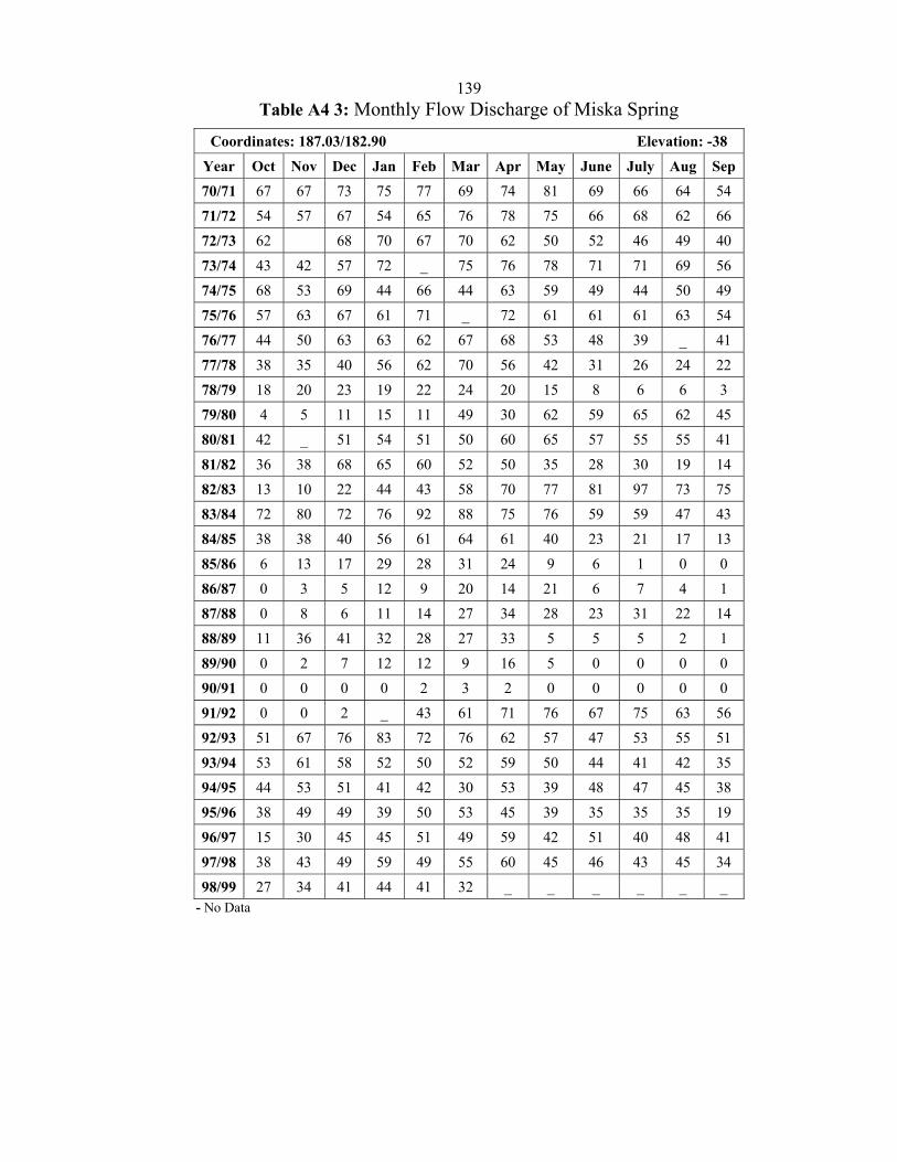
139Table A4 3: Monthly Flow Discharge of Miska Spring
Coordinates: 187.03/182.90 Elevation: -38
Year Oct Nov Dec Jan Feb Mar Apr May June July Aug Sep 70/71 67 67 73 75 77 69 74 81 69 66 64 54
71/72 54 57 67 54 65 76 78 75 66 68 62 66
72/73 62 68 70 67 70 62 50 52 46 49 40
73/74 43 42 57 72 _ 75 76 78 71 71 69 56
74/75 68 53 69 44 66 44 63 59 49 44 50 49
75/76 57 63 67 61 71 _ 72 61 61 61 63 54
76/77 44 50 63 63 62 67 68 53 48 39 _ 41
77/78 38 35 40 56 62 70 56 42 31 26 24 22
78/79 18 20 23 19 22 24 20 15 8 6 6 3
79/80 4 5 11 15 11 49 30 62 59 65 62 45
80/81 42 _ 51 54 51 50 60 65 57 55 55 41
81/82 36 38 68 65 60 52 50 35 28 30 19 14
82/83 13 10 22 44 43 58 70 77 81 97 73 75
83/84 72 80 72 76 92 88 75 76 59 59 47 43
84/85 38 38 40 56 61 64 61 40 23 21 17 13
85/86 6 13 17 29 28 31 24 9 6 1 0 0
86/87 0 3 5 12 9 20 14 21 6 7 4 1
87/88 0 8 6 11 14 27 34 28 23 31 22 14
88/89 11 36 41 32 28 27 33 5 5 5 2 1
89/90 0 2 7 12 12 9 16 5 0 0 0 0
90/91 0 0 0 0 2 3 2 0 0 0 0 0
91/92 0 0 2 _ 43 61 71 76 67 75 63 56
92/93 51 67 76 83 72 76 62 57 47 53 55 51
93/94 53 61 58 52 50 52 59 50 44 41 42 35
94/95 44 53 51 41 42 30 53 39 48 47 45 38
95/96 38 49 49 39 50 53 45 39 35 35 35 19
96/97 15 30 45 45 51 49 59 42 51 40 48 41
97/98 38 43 49 59 49 55 60 45 46 43 45 34
98/99 27 34 41 44 41 32 _ _ _ _ _ _ - No Data
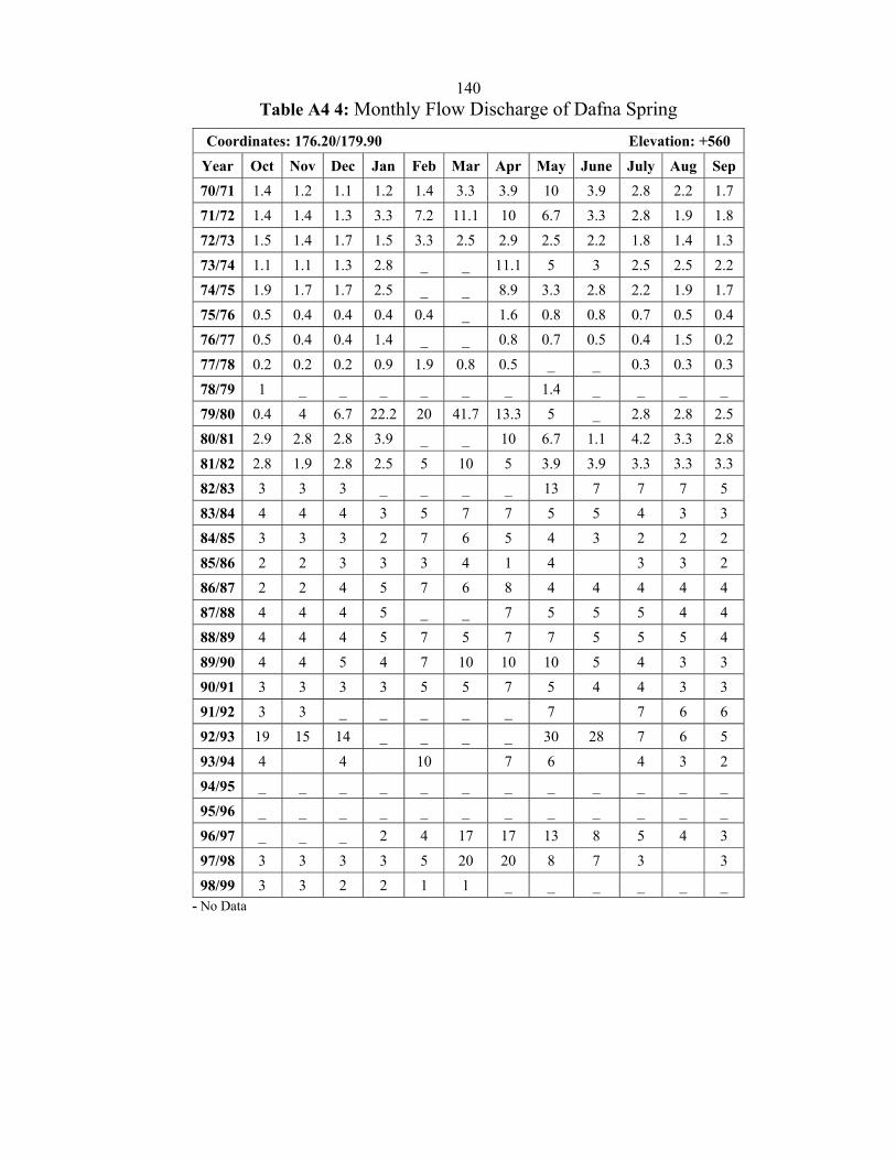
140Table A4 4: Monthly Flow Discharge of Dafna Spring
Coordinates: 176.20/179.90 Elevation: +560
Year Oct Nov Dec Jan Feb Mar Apr May June July Aug Sep 70/71 1.4 1.2 1.1 1.2 1.4 3.3 3.9 10 3.9 2.8 2.2 1.7
71/72 1.4 1.4 1.3 3.3 7.2 11.1 10 6.7 3.3 2.8 1.9 1.8
72/73 1.5 1.4 1.7 1.5 3.3 2.5 2.9 2.5 2.2 1.8 1.4 1.3
73/74 1.1 1.1 1.3 2.8 _ _ 11.1 5 3 2.5 2.5 2.2
74/75 1.9 1.7 1.7 2.5 _ _ 8.9 3.3 2.8 2.2 1.9 1.7
75/76 0.5 0.4 0.4 0.4 0.4 _ 1.6 0.8 0.8 0.7 0.5 0.4
76/77 0.5 0.4 0.4 1.4 _ _ 0.8 0.7 0.5 0.4 1.5 0.2
77/78 0.2 0.2 0.2 0.9 1.9 0.8 0.5 _ _ 0.3 0.3 0.3
78/79 1 _ _ _ _ _ _ 1.4 _ _ _ _
79/80 0.4 4 6.7 22.2 20 41.7 13.3 5 _ 2.8 2.8 2.5
80/81 2.9 2.8 2.8 3.9 _ _ 10 6.7 1.1 4.2 3.3 2.8
81/82 2.8 1.9 2.8 2.5 5 10 5 3.9 3.9 3.3 3.3 3.3
82/83 3 3 3 _ _ _ _ 13 7 7 7 5
83/84 4 4 4 3 5 7 7 5 5 4 3 3
84/85 3 3 3 2 7 6 5 4 3 2 2 2
85/86 2 2 3 3 3 4 1 4 3 3 2
86/87 2 2 4 5 7 6 8 4 4 4 4 4
87/88 4 4 4 5 _ _ 7 5 5 5 4 4
88/89 4 4 4 5 7 5 7 7 5 5 5 4
89/90 4 4 5 4 7 10 10 10 5 4 3 3
90/91 3 3 3 3 5 5 7 5 4 4 3 3
91/92 3 3 _ _ _ _ _ 7 7 6 6
92/93 19 15 14 _ _ _ _ 30 28 7 6 5
93/94 4 4 10 7 6 4 3 2
94/95 _ _ _ _ _ _ _ _ _ _ _ _
95/96 _ _ _ _ _ _ _ _ _ _ _ _
96/97 _ _ _ 2 4 17 17 13 8 5 4 3
97/98 3 3 3 3 5 20 20 8 7 3 3
98/99 3 3 2 2 1 1 _ _ _ _ _ _ - No Data
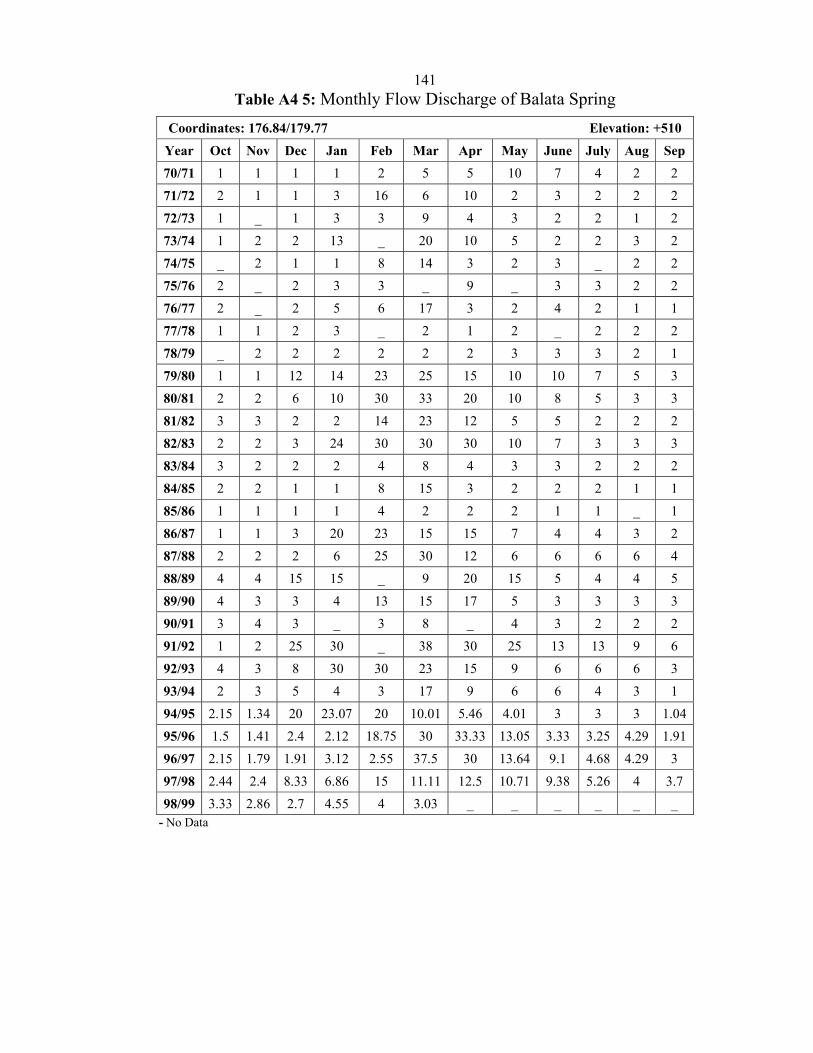
141Table A4 5: Monthly Flow Discharge of Balata Spring
Coordinates: 176.84/179.77 Elevation: +510
Year Oct Nov Dec Jan Feb Mar Apr May June July Aug Sep 70/71 1 1 1 1 2 5 5 10 7 4 2 2
71/72 2 1 1 3 16 6 10 2 3 2 2 2
72/73 1 _ 1 3 3 9 4 3 2 2 1 2
73/74 1 2 2 13 _ 20 10 5 2 2 3 2
74/75 _ 2 1 1 8 14 3 2 3 _ 2 2
75/76 2 _ 2 3 3 _ 9 _ 3 3 2 2
76/77 2 _ 2 5 6 17 3 2 4 2 1 1
77/78 1 1 2 3 _ 2 1 2 _ 2 2 2
78/79 _ 2 2 2 2 2 2 3 3 3 2 1
79/80 1 1 12 14 23 25 15 10 10 7 5 3
80/81 2 2 6 10 30 33 20 10 8 5 3 3
81/82 3 3 2 2 14 23 12 5 5 2 2 2
82/83 2 2 3 24 30 30 30 10 7 3 3 3
83/84 3 2 2 2 4 8 4 3 3 2 2 2
84/85 2 2 1 1 8 15 3 2 2 2 1 1
85/86 1 1 1 1 4 2 2 2 1 1 _ 1
86/87 1 1 3 20 23 15 15 7 4 4 3 2
87/88 2 2 2 6 25 30 12 6 6 6 6 4
88/89 4 4 15 15 _ 9 20 15 5 4 4 5
89/90 4 3 3 4 13 15 17 5 3 3 3 3
90/91 3 4 3 _ 3 8 _ 4 3 2 2 2
91/92 1 2 25 30 _ 38 30 25 13 13 9 6
92/93 4 3 8 30 30 23 15 9 6 6 6 3
93/94 2 3 5 4 3 17 9 6 6 4 3 1
94/95 2.15 1.34 20 23.07 20 10.01 5.46 4.01 3 3 3 1.04
95/96 1.5 1.41 2.4 2.12 18.75 30 33.33 13.05 3.33 3.25 4.29 1.91
96/97 2.15 1.79 1.91 3.12 2.55 37.5 30 13.64 9.1 4.68 4.29 3
97/98 2.44 2.4 8.33 6.86 15 11.11 12.5 10.71 9.38 5.26 4 3.7
98/99 3.33 2.86 2.7 4.55 4 3.03 _ _ _ _ _ _ - No Data
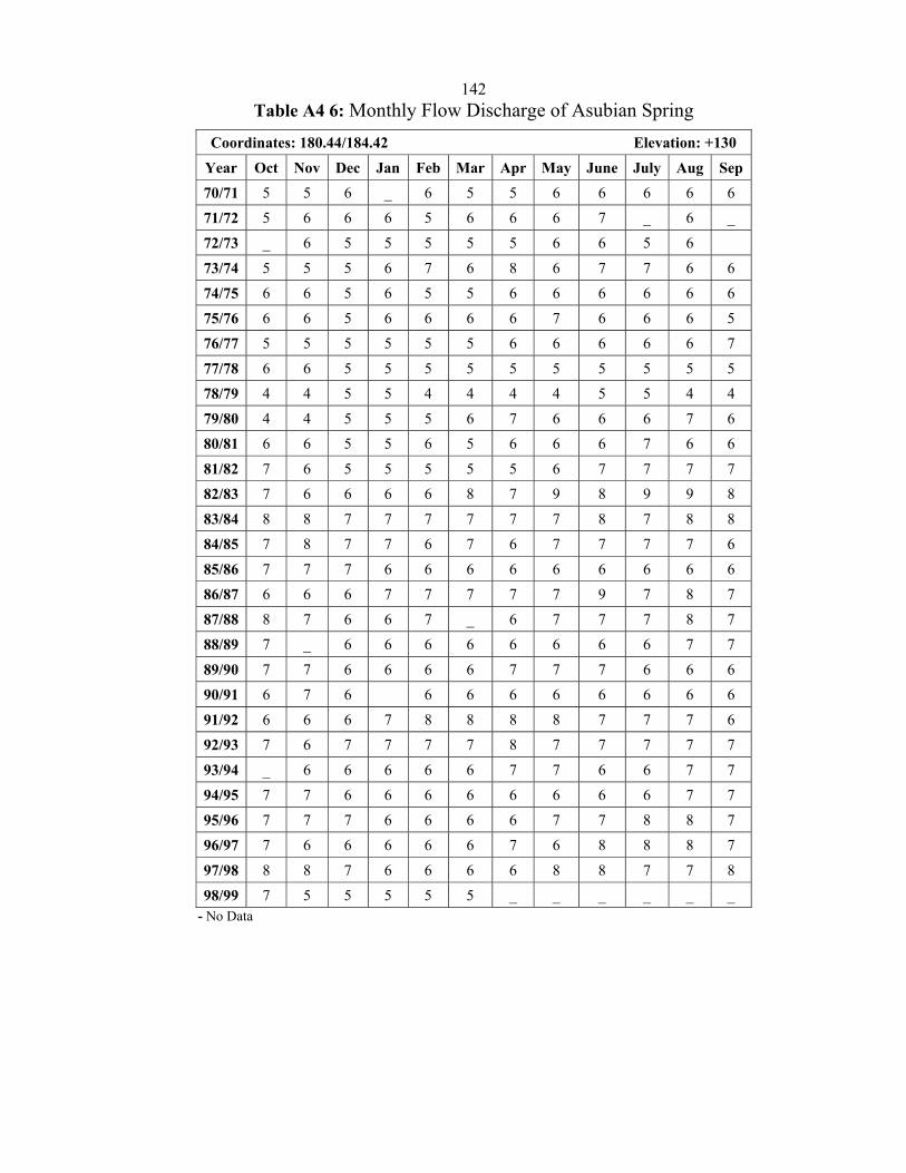
142Table A4 6: Monthly Flow Discharge of Asubian Spring
Coordinates: 180.44/184.42 Elevation: +130
Year Oct Nov Dec Jan Feb Mar Apr May June July Aug Sep 70/71 5 5 6 _ 6 5 5 6 6 6 6 6
71/72 5 6 6 6 5 6 6 6 7 _ 6 _
72/73 _ 6 5 5 5 5 5 6 6 5 6
73/74 5 5 5 6 7 6 8 6 7 7 6 6
74/75 6 6 5 6 5 5 6 6 6 6 6 6
75/76 6 6 5 6 6 6 6 7 6 6 6 5
76/77 5 5 5 5 5 5 6 6 6 6 6 7
77/78 6 6 5 5 5 5 5 5 5 5 5 5
78/79 4 4 5 5 4 4 4 4 5 5 4 4
79/80 4 4 5 5 5 6 7 6 6 6 7 6
80/81 6 6 5 5 6 5 6 6 6 7 6 6
81/82 7 6 5 5 5 5 5 6 7 7 7 7
82/83 7 6 6 6 6 8 7 9 8 9 9 8
83/84 8 8 7 7 7 7 7 7 8 7 8 8
84/85 7 8 7 7 6 7 6 7 7 7 7 6
85/86 7 7 7 6 6 6 6 6 6 6 6 6
86/87 6 6 6 7 7 7 7 7 9 7 8 7
87/88 8 7 6 6 7 _ 6 7 7 7 8 7
88/89 7 _ 6 6 6 6 6 6 6 6 7 7
89/90 7 7 6 6 6 6 7 7 7 6 6 6
90/91 6 7 6 6 6 6 6 6 6 6 6
91/92 6 6 6 7 8 8 8 8 7 7 7 6
92/93 7 6 7 7 7 7 8 7 7 7 7 7
93/94 _ 6 6 6 6 6 7 7 6 6 7 7
94/95 7 7 6 6 6 6 6 6 6 6 7 7
95/96 7 7 7 6 6 6 6 7 7 8 8 7
96/97 7 6 6 6 6 6 7 6 8 8 8 7
97/98 8 8 7 6 6 6 6 8 8 7 7 8
98/99 7 5 5 5 5 5 _ _ _ _ _ _ - No Data
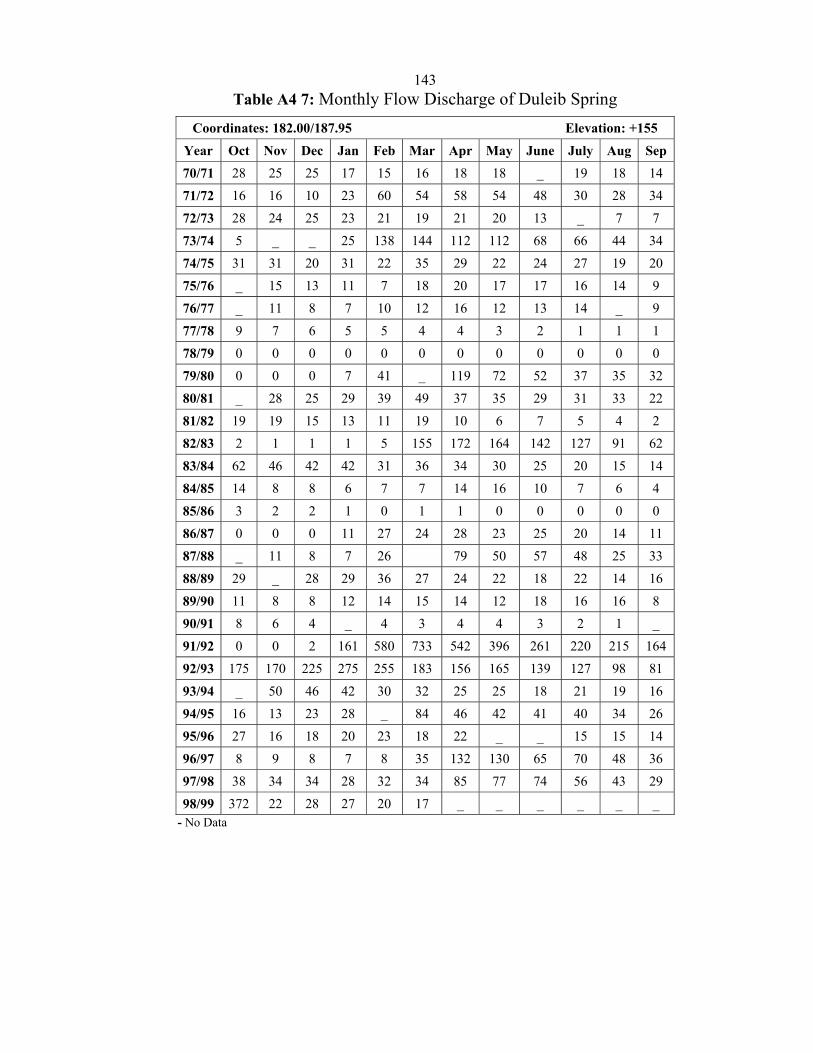
143Table A4 7: Monthly Flow Discharge of Duleib Spring
Coordinates: 182.00/187.95 Elevation: +155
Year Oct Nov Dec Jan Feb Mar Apr May June July Aug Sep 70/71 28 25 25 17 15 16 18 18 _ 19 18 14
71/72 16 16 10 23 60 54 58 54 48 30 28 34
72/73 28 24 25 23 21 19 21 20 13 _ 7 7
73/74 5 _ _ 25 138 144 112 112 68 66 44 34
74/75 31 31 20 31 22 35 29 22 24 27 19 20
75/76 _ 15 13 11 7 18 20 17 17 16 14 9
76/77 _ 11 8 7 10 12 16 12 13 14 _ 9
77/78 9 7 6 5 5 4 4 3 2 1 1 1
78/79 0 0 0 0 0 0 0 0 0 0 0 0
79/80 0 0 0 7 41 _ 119 72 52 37 35 32
80/81 _ 28 25 29 39 49 37 35 29 31 33 22
81/82 19 19 15 13 11 19 10 6 7 5 4 2
82/83 2 1 1 1 5 155 172 164 142 127 91 62
83/84 62 46 42 42 31 36 34 30 25 20 15 14
84/85 14 8 8 6 7 7 14 16 10 7 6 4
85/86 3 2 2 1 0 1 1 0 0 0 0 0
86/87 0 0 0 11 27 24 28 23 25 20 14 11
87/88 _ 11 8 7 26 79 50 57 48 25 33
88/89 29 _ 28 29 36 27 24 22 18 22 14 16
89/90 11 8 8 12 14 15 14 12 18 16 16 8
90/91 8 6 4 _ 4 3 4 4 3 2 1 _
91/92 0 0 2 161 580 733 542 396 261 220 215 164
92/93 175 170 225 275 255 183 156 165 139 127 98 81
93/94 _ 50 46 42 30 32 25 25 18 21 19 16
94/95 16 13 23 28 _ 84 46 42 41 40 34 26
95/96 27 16 18 20 23 18 22 _ _ 15 15 14
96/97 8 9 8 7 8 35 132 130 65 70 48 36
97/98 38 34 34 28 32 34 85 77 74 56 43 29
98/99 372 22 28 27 20 17 _ _ _ _ _ _ - No Data
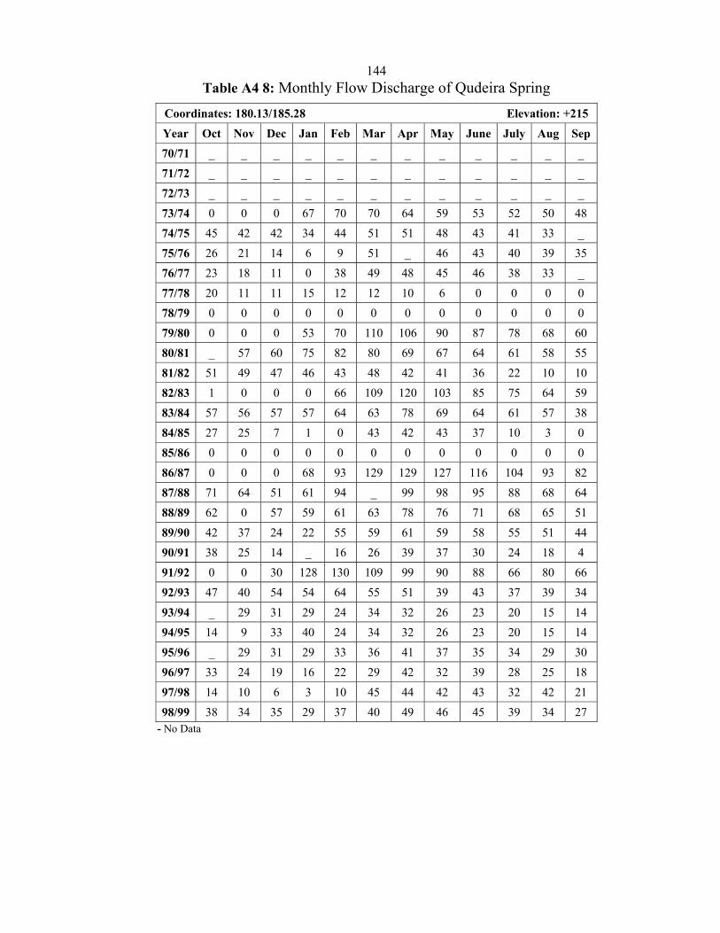
144Table A4 8: Monthly Flow Discharge of Qudeira Spring
Coordinates: 180.13/185.28 Elevation: +215
Year Oct Nov Dec Jan Feb Mar Apr May June July Aug Sep 70/71 _ _ _ _ _ _ _ _ _ _ _ _
71/72 _ _ _ _ _ _ _ _ _ _ _ _
72/73 _ _ _ _ _ _ _ _ _ _ _ _
73/74 0 0 0 67 70 70 64 59 53 52 50 48
74/75 45 42 42 34 44 51 51 48 43 41 33 _
75/76 26 21 14 6 9 51 _ 46 43 40 39 35
76/77 23 18 11 0 38 49 48 45 46 38 33 _
77/78 20 11 11 15 12 12 10 6 0 0 0 0
78/79 0 0 0 0 0 0 0 0 0 0 0 0
79/80 0 0 0 53 70 110 106 90 87 78 68 60
80/81 _ 57 60 75 82 80 69 67 64 61 58 55
81/82 51 49 47 46 43 48 42 41 36 22 10 10
82/83 1 0 0 0 66 109 120 103 85 75 64 59
83/84 57 56 57 57 64 63 78 69 64 61 57 38
84/85 27 25 7 1 0 43 42 43 37 10 3 0
85/86 0 0 0 0 0 0 0 0 0 0 0 0
86/87 0 0 0 68 93 129 129 127 116 104 93 82
87/88 71 64 51 61 94 _ 99 98 95 88 68 64
88/89 62 0 57 59 61 63 78 76 71 68 65 51
89/90 42 37 24 22 55 59 61 59 58 55 51 44
90/91 38 25 14 _ 16 26 39 37 30 24 18 4
91/92 0 0 30 128 130 109 99 90 88 66 80 66
92/93 47 40 54 54 64 55 51 39 43 37 39 34
93/94 _ 29 31 29 24 34 32 26 23 20 15 14
94/95 14 9 33 40 24 34 32 26 23 20 15 14
95/96 _ 29 31 29 33 36 41 37 35 34 29 30
96/97 33 24 19 16 22 29 42 32 39 28 25 18
97/98 14 10 6 3 10 45 44 42 43 32 42 21
98/99 38 34 35 29 37 40 49 46 45 39 34 27 - No Data
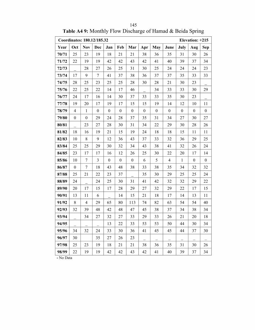
145Table A4 9: Monthly Flow Discharge of Hamad & Beida Spring
Coordinates: 180.12/185.32 Elevation: +215
Year Oct Nov Dec Jan Feb Mar Apr May June July Aug Sep 70/71 25 23 19 18 21 21 38 36 35 31 30 26
71/72 22 19 19 42 42 43 42 41 40 39 37 34
72/73 _ 28 27 26 25 31 30 25 24 24 24 23
73/74 17 9 7 41 37 38 36 37 37 35 33 33
74/75 28 25 23 25 25 28 30 28 21 30 23 _
75/76 22 25 22 14 17 46 _ 34 33 33 30 29
76/77 24 17 16 14 30 37 33 33 35 30 23 _
77/78 19 20 17 19 17 15 15 19 14 12 10 11
78/79 4 1 0 0 0 0 0 0 0 0 0 0
79/80 0 0 29 24 28 37 35 31 34 27 30 27
80/81 _ 23 27 28 30 31 34 22 29 30 28 26
81/82 18 16 19 21 15 19 24 18 18 15 11 11
82/83 10 8 9 12 36 43 37 33 32 36 29 25
83/84 25 25 29 30 32 34 43 38 41 32 26 24
84/85 23 17 17 16 12 26 25 30 22 20 17 14
85/86 10 7 3 0 0 0 6 5 4 1 0 0
86/87 0 7 18 43 48 38 33 38 35 34 32 32
87/88 25 21 22 23 37 _ 35 30 29 25 25 24
88/89 24 _ 24 25 30 31 41 42 32 32 29 22
89/90 20 17 15 17 28 29 27 32 29 22 17 15
90/91 13 11 6 _ 14 15 21 18 17 14 13 11
91/92 8 4 29 65 80 113 74 82 63 54 54 40
92/93 32 39 48 42 48 47 45 38 37 34 38 34
93/94 _ 34 27 32 27 33 29 33 26 21 20 18
94/95 _ _ _ 13 22 33 53 53 50 44 30 34
95/96 34 32 24 33 30 36 41 45 45 44 37 30
96/97 30 35 27 26 23 _ _ _ _ _ _
97/98 25 23 19 18 21 21 38 36 35 31 30 26
98/99 22 19 19 42 42 43 42 41 40 39 37 34 - No Data
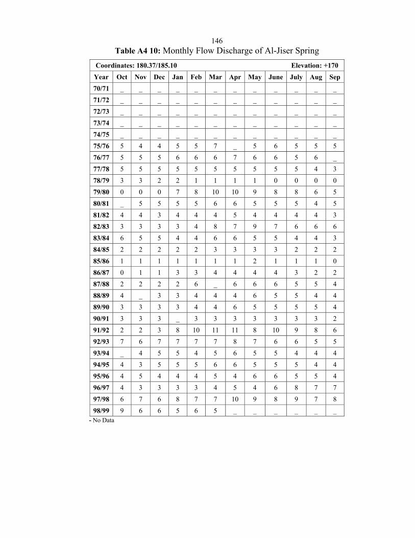
146Table A4 10: Monthly Flow Discharge of Al-Jiser Spring
Coordinates: 180.37/185.10 Elevation: +170
Year Oct Nov Dec Jan Feb Mar Apr May June July Aug Sep 70/71 _ _ _ _ _ _ _ _ _ _ _ _
71/72 _ _ _ _ _ _ _ _ _ _ _ _
72/73 _ _ _ _ _ _ _ _ _ _ _ _
73/74 _ _ _ _ _ _ _ _ _ _ _ _
74/75 _ _ _ _ _ _ _ _ _ _ _ _
75/76 5 4 4 5 5 7 _ 5 6 5 5 5
76/77 5 5 5 6 6 6 7 6 6 5 6 _
77/78 5 5 5 5 5 5 5 5 5 5 4 3
78/79 3 3 2 2 1 1 1 1 0 0 0 0
79/80 0 0 0 7 8 10 10 9 8 8 6 5
80/81 _ 5 5 5 5 6 6 5 5 5 4 5
81/82 4 4 3 4 4 4 5 4 4 4 4 3
82/83 3 3 3 3 4 8 7 9 7 6 6 6
83/84 6 5 5 4 4 6 6 5 5 4 4 3
84/85 2 2 2 2 2 3 3 3 3 2 2 2
85/86 1 1 1 1 1 1 1 2 1 1 1 0
86/87 0 1 1 3 3 4 4 4 4 3 2 2
87/88 2 2 2 2 6 _ 6 6 6 5 5 4
88/89 4 _ 3 3 4 4 4 6 5 5 4 4
89/90 3 3 3 3 4 4 6 5 5 5 5 4
90/91 3 3 3 _ 3 3 3 3 3 3 3 2
91/92 2 2 3 8 10 11 11 8 10 9 8 6
92/93 7 6 7 7 7 7 8 7 6 6 5 5
93/94 _ 4 5 5 4 5 6 5 5 4 4 4
94/95 4 3 5 5 5 6 6 5 5 5 4 4
95/96 4 5 4 4 4 5 4 6 6 5 5 4
96/97 4 3 3 3 3 4 5 4 6 8 7 7
97/98 6 7 6 8 7 7 10 9 8 9 7 8
98/99 9 6 6 5 6 5 _ _ _ _ _ _ - No Data
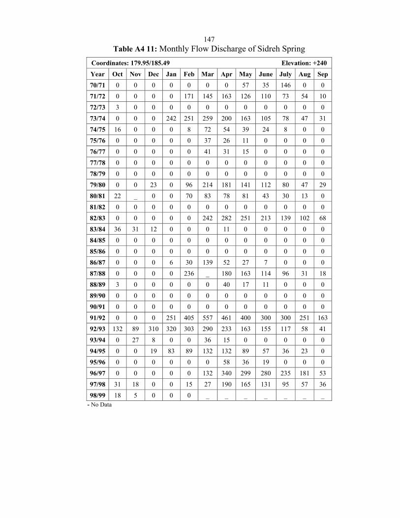
147Table A4 11: Monthly Flow Discharge of Sidreh Spring
Coordinates: 179.95/185.49 Elevation: +240
Year Oct Nov Dec Jan Feb Mar Apr May June July Aug Sep 70/71 0 0 0 0 0 0 0 57 35 146 0 0
71/72 0 0 0 0 171 145 163 126 110 73 54 10
72/73 3 0 0 0 0 0 0 0 0 0 0 0
73/74 0 0 0 242 251 259 200 163 105 78 47 31
74/75 16 0 0 0 8 72 54 39 24 8 0 0
75/76 0 0 0 0 0 37 26 11 0 0 0 0
76/77 0 0 0 0 0 41 31 15 0 0 0 0
77/78 0 0 0 0 0 0 0 0 0 0 0 0
78/79 0 0 0 0 0 0 0 0 0 0 0 0
79/80 0 0 23 0 96 214 181 141 112 80 47 29
80/81 22 _ 0 0 70 83 78 81 43 30 13 0
81/82 0 0 0 0 0 0 0 0 0 0 0 0
82/83 0 0 0 0 0 242 282 251 213 139 102 68
83/84 36 31 12 0 0 0 11 0 0 0 0 0
84/85 0 0 0 0 0 0 0 0 0 0 0 0
85/86 0 0 0 0 0 0 0 0 0 0 0 0
86/87 0 0 0 6 30 139 52 27 7 0 0 0
87/88 0 0 0 0 236 _ 180 163 114 96 31 18
88/89 3 0 0 0 0 0 40 17 11 0 0 0
89/90 0 0 0 0 0 0 0 0 0 0 0 0
90/91 0 0 0 0 0 0 0 0 0 0 0 0
91/92 0 0 0 251 405 557 461 400 300 300 251 163
92/93 132 89 310 320 303 290 233 163 155 117 58 41
93/94 0 27 8 0 0 36 15 0 0 0 0 0
94/95 0 0 19 83 89 132 132 89 57 36 23 0
95/96 0 0 0 0 0 0 58 36 19 0 0 0
96/97 0 0 0 0 0 132 340 299 280 235 181 53
97/98 31 18 0 0 15 27 190 165 131 95 57 36
98/99 18 5 0 0 0 _ _ _ _ _ _ _ - No Data
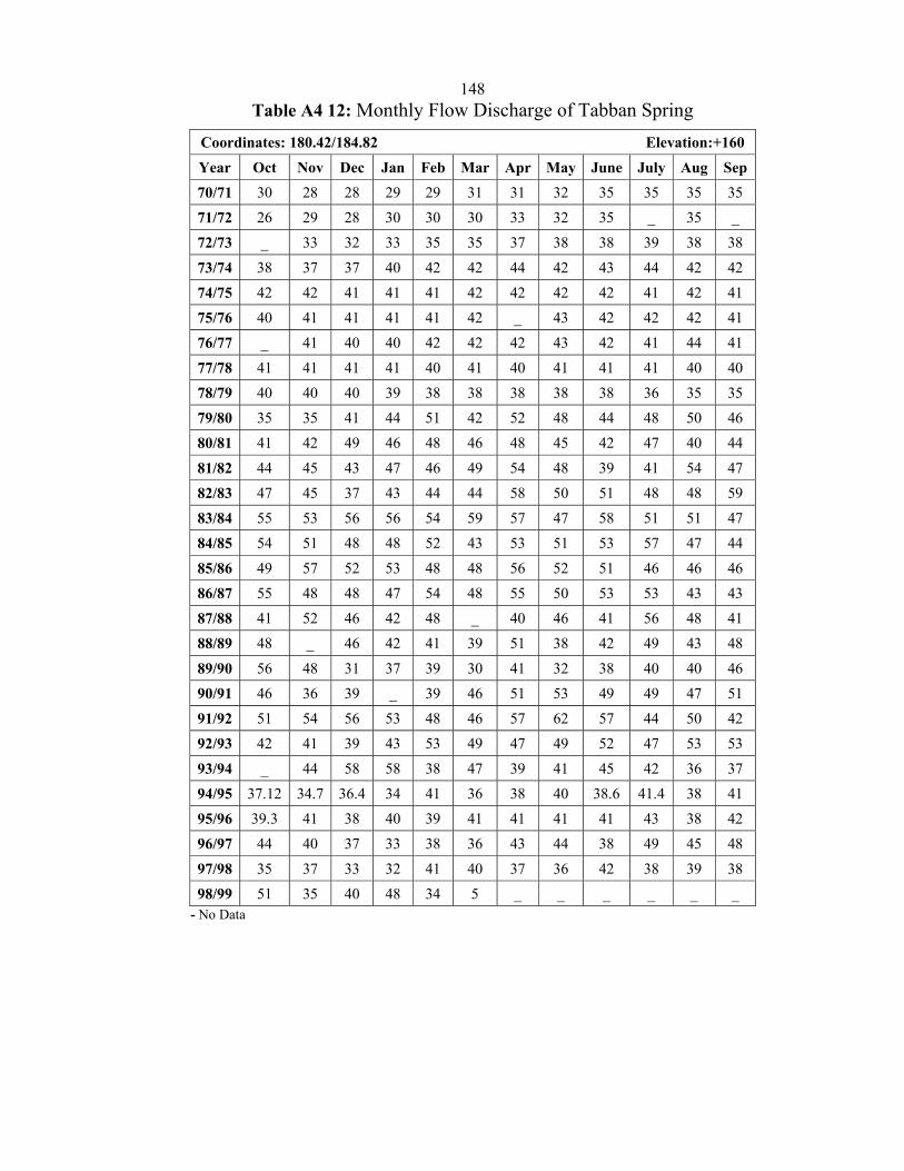
148Table A4 12: Monthly Flow Discharge of Tabban Spring
Coordinates: 180.42/184.82 Elevation:+160
Year Oct Nov Dec Jan Feb Mar Apr May June July Aug Sep 70/71 30 28 28 29 29 31 31 32 35 35 35 35
71/72 26 29 28 30 30 30 33 32 35 _ 35 _
72/73 _ 33 32 33 35 35 37 38 38 39 38 38
73/74 38 37 37 40 42 42 44 42 43 44 42 42
74/75 42 42 41 41 41 42 42 42 42 41 42 41
75/76 40 41 41 41 41 42 _ 43 42 42 42 41
76/77 _ 41 40 40 42 42 42 43 42 41 44 41
77/78 41 41 41 41 40 41 40 41 41 41 40 40
78/79 40 40 40 39 38 38 38 38 38 36 35 35
79/80 35 35 41 44 51 42 52 48 44 48 50 46
80/81 41 42 49 46 48 46 48 45 42 47 40 44
81/82 44 45 43 47 46 49 54 48 39 41 54 47
82/83 47 45 37 43 44 44 58 50 51 48 48 59
83/84 55 53 56 56 54 59 57 47 58 51 51 47
84/85 54 51 48 48 52 43 53 51 53 57 47 44
85/86 49 57 52 53 48 48 56 52 51 46 46 46
86/87 55 48 48 47 54 48 55 50 53 53 43 43
87/88 41 52 46 42 48 _ 40 46 41 56 48 41
88/89 48 _ 46 42 41 39 51 38 42 49 43 48
89/90 56 48 31 37 39 30 41 32 38 40 40 46
90/91 46 36 39 _ 39 46 51 53 49 49 47 51
91/92 51 54 56 53 48 46 57 62 57 44 50 42
92/93 42 41 39 43 53 49 47 49 52 47 53 53
93/94 _ 44 58 58 38 47 39 41 45 42 36 37
94/95 37.12 34.7 36.4 34 41 36 38 40 38.6 41.4 38 41
95/96 39.3 41 38 40 39 41 41 41 41 43 38 42
96/97 44 40 37 33 38 36 43 44 38 49 45 48
97/98 35 37 33 32 41 40 37 36 42 38 39 38
98/99 51 35 40 48 34 5 _ _ _ _ _ _ - No Data
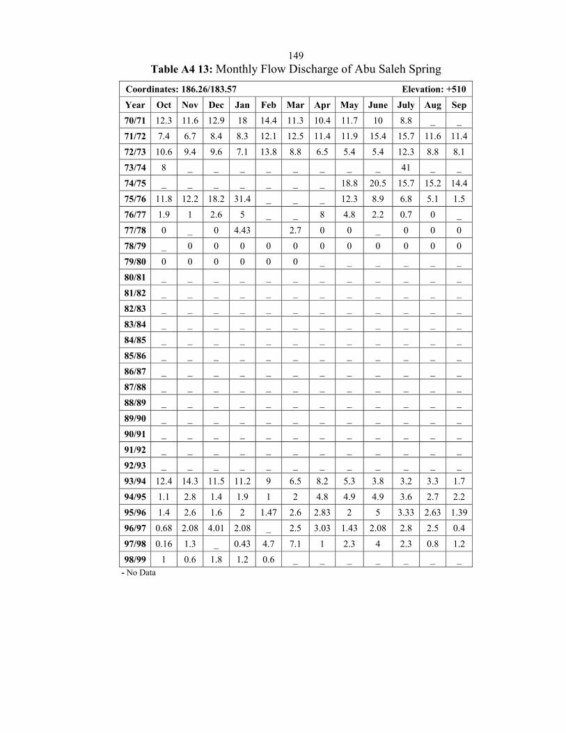
149Table A4 13: Monthly Flow Discharge of Abu Saleh Spring
Coordinates: 186.26/183.57 Elevation: +510
Year Oct Nov Dec Jan Feb Mar Apr May June July Aug Sep 70/71 12.3 11.6 12.9 18 14.4 11.3 10.4 11.7 10 8.8 _ _
71/72 7.4 6.7 8.4 8.3 12.1 12.5 11.4 11.9 15.4 15.7 11.6 11.4
72/73 10.6 9.4 9.6 7.1 13.8 8.8 6.5 5.4 5.4 12.3 8.8 8.1
73/74 8 _ _ _ _ _ _ _ _ 41 _ _
74/75 _ _ _ _ _ _ _ 18.8 20.5 15.7 15.2 14.4
75/76 11.8 12.2 18.2 31.4 _ _ _ 12.3 8.9 6.8 5.1 1.5
76/77 1.9 1 2.6 5 _ _ 8 4.8 2.2 0.7 0 _
77/78 0 _ 0 4.43 2.7 0 0 _ 0 0 0
78/79 _ 0 0 0 0 0 0 0 0 0 0 0
79/80 0 0 0 0 0 0 _ _ _ _ _ _
80/81 _ _ _ _ _ _ _ _ _ _ _ _
81/82 _ _ _ _ _ _ _ _ _ _ _ _
82/83 _ _ _ _ _ _ _ _ _ _ _ _
83/84 _ _ _ _ _ _ _ _ _ _ _ _
84/85 _ _ _ _ _ _ _ _ _ _ _ _
85/86 _ _ _ _ _ _ _ _ _ _ _ _
86/87 _ _ _ _ _ _ _ _ _ _ _ _
87/88 _ _ _ _ _ _ _ _ _ _ _ _
88/89 _ _ _ _ _ _ _ _ _ _ _ _
89/90 _ _ _ _ _ _ _ _ _ _ _ _
90/91 _ _ _ _ _ _ _ _ _ _ _ _
91/92 _ _ _ _ _ _ _ _ _ _ _ _
92/93 _ _ _ _ _ _ _ _ _ _ _ _
93/94 12.4 14.3 11.5 11.2 9 6.5 8.2 5.3 3.8 3.2 3.3 1.7
94/95 1.1 2.8 1.4 1.9 1 2 4.8 4.9 4.9 3.6 2.7 2.2
95/96 1.4 2.6 1.6 2 1.47 2.6 2.83 2 5 3.33 2.63 1.39
96/97 0.68 2.08 4.01 2.08 _ 2.5 3.03 1.43 2.08 2.8 2.5 0.4
97/98 0.16 1.3 _ 0.43 4.7 7.1 1 2.3 4 2.3 0.8 1.2
98/99 1 0.6 1.8 1.2 0.6 _ _ _ _ _ _ _ - No Data
150
APPENDIX A5
FLOW MEASUREMENTS AT WADI AL-BADAN AND WADI AL-FARIA
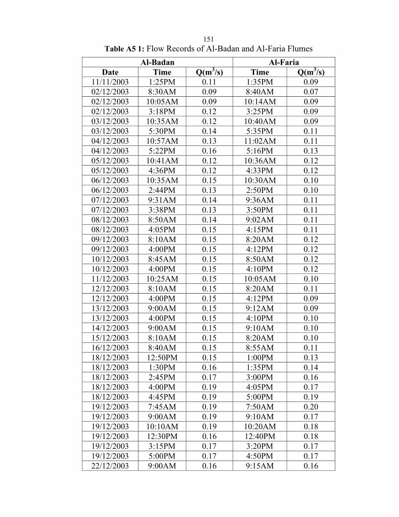
151Table A5 1: Flow Records of Al-Badan and Al-Faria Flumes
Al-Badan Al-Faria Date Time Q(m3/s) Time Q(m3/s)
11/11/2003 1:25PM 0.11 1:35PM 0.09 02/12/2003 8:30AM 0.09 8:40AM 0.07 02/12/2003 10:05AM 0.09 10:14AM 0.09 02/12/2003 3:18PM 0.12 3:25PM 0.09 03/12/2003 10:35AM 0.12 10:40AM 0.09 03/12/2003 5:30PM 0.14 5:35PM 0.11 04/12/2003 10:57AM 0.13 11:02AM 0.11 04/12/2003 5:22PM 0.16 5:16PM 0.13 05/12/2003 10:41AM 0.12 10:36AM 0.12 05/12/2003 4:36PM 0.12 4:33PM 0.12 06/12/2003 10:35AM 0.15 10:30AM 0.10 06/12/2003 2:44PM 0.13 2:50PM 0.10 07/12/2003 9:31AM 0.14 9:36AM 0.11 07/12/2003 3:38PM 0.13 3:50PM 0.11 08/12/2003 8:50AM 0.14 9:02AM 0.11 08/12/2003 4:05PM 0.15 4:15PM 0.11 09/12/2003 8:10AM 0.15 8:20AM 0.12 09/12/2003 4:00PM 0.15 4:12PM 0.12 10/12/2003 8:45AM 0.15 8:50AM 0.12 10/12/2003 4:00PM 0.15 4:10PM 0.12 11/12/2003 10:25AM 0.15 10:05AM 0.10 12/12/2003 8:10AM 0.15 8:20AM 0.11 12/12/2003 4:00PM 0.15 4:12PM 0.09 13/12/2003 9:00AM 0.15 9:12AM 0.09 13/12/2003 4:00PM 0.15 4:10PM 0.10 14/12/2003 9:00AM 0.15 9:10AM 0.10 15/12/2003 8:10AM 0.15 8:20AM 0.10 16/12/2003 8:40AM 0.15 8:55AM 0.11 18/12/2003 12:50PM 0.15 1:00PM 0.13 18/12/2003 1:30PM 0.16 1:35PM 0.14 18/12/2003 2:45PM 0.17 3:00PM 0.16 18/12/2003 4:00PM 0.19 4:05PM 0.17 18/12/2003 4:45PM 0.19 5:00PM 0.19 19/12/2003 7:45AM 0.19 7:50AM 0.20 19/12/2003 9:00AM 0.19 9:10AM 0.17 19/12/2003 10:10AM 0.19 10:20AM 0.18 19/12/2003 12:30PM 0.16 12:40PM 0.18 19/12/2003 3:15PM 0.17 3:20PM 0.17 19/12/2003 5:00PM 0.17 4:50PM 0.17 22/12/2003 9:00AM 0.16 9:15AM 0.16
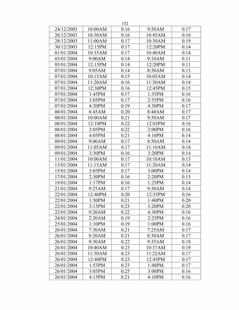
15224/12/2003 10:00AM 0.16 9:50AM 0.17 26/12/2003 10:30AM 0.16 10:45AM 0.16 28/12/2003 11:00AM 0.17 10:30AM 0.19 30/12/2003 12:15PM 0.17 12:20PM 0.14 01/01/2004 10:35AM 0.17 10:40AM 0.14 03/01/2004 9:00AM 0.14 9:10AM 0.11 05/01/2004 12:15PM 0.14 12:20PM 0.11 07/01/2004 9:05AM 0.14 8:50AM 0.13 07/01/2004 10:15AM 0.15 10:05AM 0.14 07/01/2004 11:20AM 0.16 11:30AM 0.14 07/01/2004 12:30PM 0.16 12:45PM 0.15 07/01/2004 1:45PM 0.17 1:35PM 0.16 07/01/2004 3:05PM 0.17 2:55PM 0.16 07/01/2004 4:20PM 0.19 4:30PM 0.17 08/01/2004 8:45AM 0.20 8:40AM 0.17 08/01/2004 10:00AM 0.21 9:50AM 0.17 08/01/2004 12:10PM 0.22 12:03PM 0.16 08/01/2004 2:05PM 0.22 2:00PM 0.16 08/01/2004 4:05PM 0.21 4:10PM 0.14 09/01/2004 9:00AM 0.17 8:50AM 0.14 09/01/2004 11:05AM 0.17 11:10AM 0.14 09/01/2004 3:30PM 0.16 3:20PM 0.14 11/01/2004 10:00AM 0.17 10:10AM 0.13 13/01/2004 11:15AM 0.17 11:20AM 0.14 15/01/2004 3:05PM 0.17 3:00PM 0.14 17/01/2004 2:30PM 0.16 2:20PM 0.13 19/01/2004 1:17PM 0.16 1:25PM 0.14 21/01/2004 9:25AM 0.17 9:30AM 0.14 22/01/2004 12:40PM 0.20 12:35PM 0.16 22/01/2004 1:50PM 0.21 1:40PM 0.20 22/01/2004 3:15PM 0.23 3:20PM 0.20 22/01/2004 9:20AM 0.22 4:30PM 0.16 24/01/2004 2:20AM 0.19 2:25PM 0.16 25/01/2004 1:10PM 0.19 1:00PM 0.16 26/01/2004 7:30AM 0.21 7:25AM 0.17 26/01/2004 8:20AM 0.21 8:30AM 0.17 26/01/2004 9:30AM 0.22 9:35AM 0.18 26/01/2004 10:40AM 0.23 10:37AM 0.19 26/01/2004 11:30AM 0.23 11:22AM 0.17 26/01/2004 12:40PM 0.23 12:45PM 0.17 26/01/2004 1:53PM 0.23 1:48PM 0.17 26/01/2004 3:05PM 0.25 3:00PM 0.16 26/01/2004 4:15PM 0.21 4:10PM 0.16
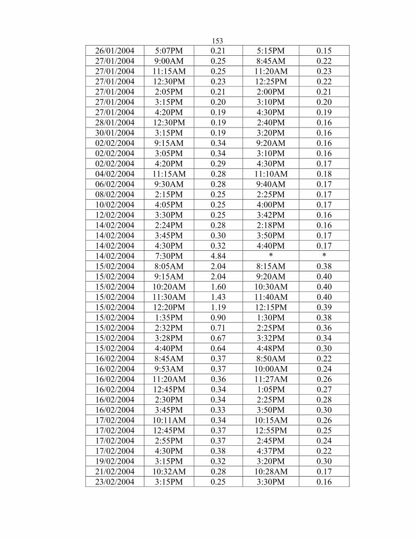
15326/01/2004 5:07PM 0.21 5:15PM 0.15 27/01/2004 9:00AM 0.25 8:45AM 0.22 27/01/2004 11:15AM 0.25 11:20AM 0.23 27/01/2004 12:30PM 0.23 12:25PM 0.22 27/01/2004 2:05PM 0.21 2:00PM 0.21 27/01/2004 3:15PM 0.20 3:10PM 0.20 27/01/2004 4:20PM 0.19 4:30PM 0.19 28/01/2004 12:30PM 0.19 2:40PM 0.16 30/01/2004 3:15PM 0.19 3:20PM 0.16 02/02/2004 9:15AM 0.34 9:20AM 0.16 02/02/2004 3:05PM 0.34 3:10PM 0.16 02/02/2004 4:20PM 0.29 4:30PM 0.17 04/02/2004 11:15AM 0.28 11:10AM 0.18 06/02/2004 9:30AM 0.28 9:40AM 0.17 08/02/2004 2:15PM 0.25 2:25PM 0.17 10/02/2004 4:05PM 0.25 4:00PM 0.17 12/02/2004 3:30PM 0.25 3:42PM 0.16 14/02/2004 2:24PM 0.28 2:18PM 0.16 14/02/2004 3:45PM 0.30 3:50PM 0.17 14/02/2004 4:30PM 0.32 4:40PM 0.17 14/02/2004 7:30PM 4.84 * * 15/02/2004 8:05AM 2.04 8:15AM 0.38 15/02/2004 9:15AM 2.04 9:20AM 0.40 15/02/2004 10:20AM 1.60 10:30AM 0.40 15/02/2004 11:30AM 1.43 11:40AM 0.40 15/02/2004 12:20PM 1.19 12:15PM 0.39 15/02/2004 1:35PM 0.90 1:30PM 0.38 15/02/2004 2:32PM 0.71 2:25PM 0.36 15/02/2004 3:28PM 0.67 3:32PM 0.34 15/02/2004 4:40PM 0.64 4:48PM 0.30 16/02/2004 8:45AM 0.37 8:50AM 0.22 16/02/2004 9:53AM 0.37 10:00AM 0.24 16/02/2004 11:20AM 0.36 11:27AM 0.26 16/02/2004 12:45PM 0.34 1:05PM 0.27 16/02/2004 2:30PM 0.34 2:25PM 0.28 16/02/2004 3:45PM 0.33 3:50PM 0.30 17/02/2004 10:11AM 0.34 10:15AM 0.26 17/02/2004 12:45PM 0.37 12:55PM 0.25 17/02/2004 2:55PM 0.37 2:45PM 0.24 17/02/2004 4:30PM 0.38 4:37PM 0.22 19/02/2004 3:15PM 0.32 3:20PM 0.30 21/02/2004 10:32AM 0.28 10:28AM 0.17 23/02/2004 3:15PM 0.25 3:30PM 0.16
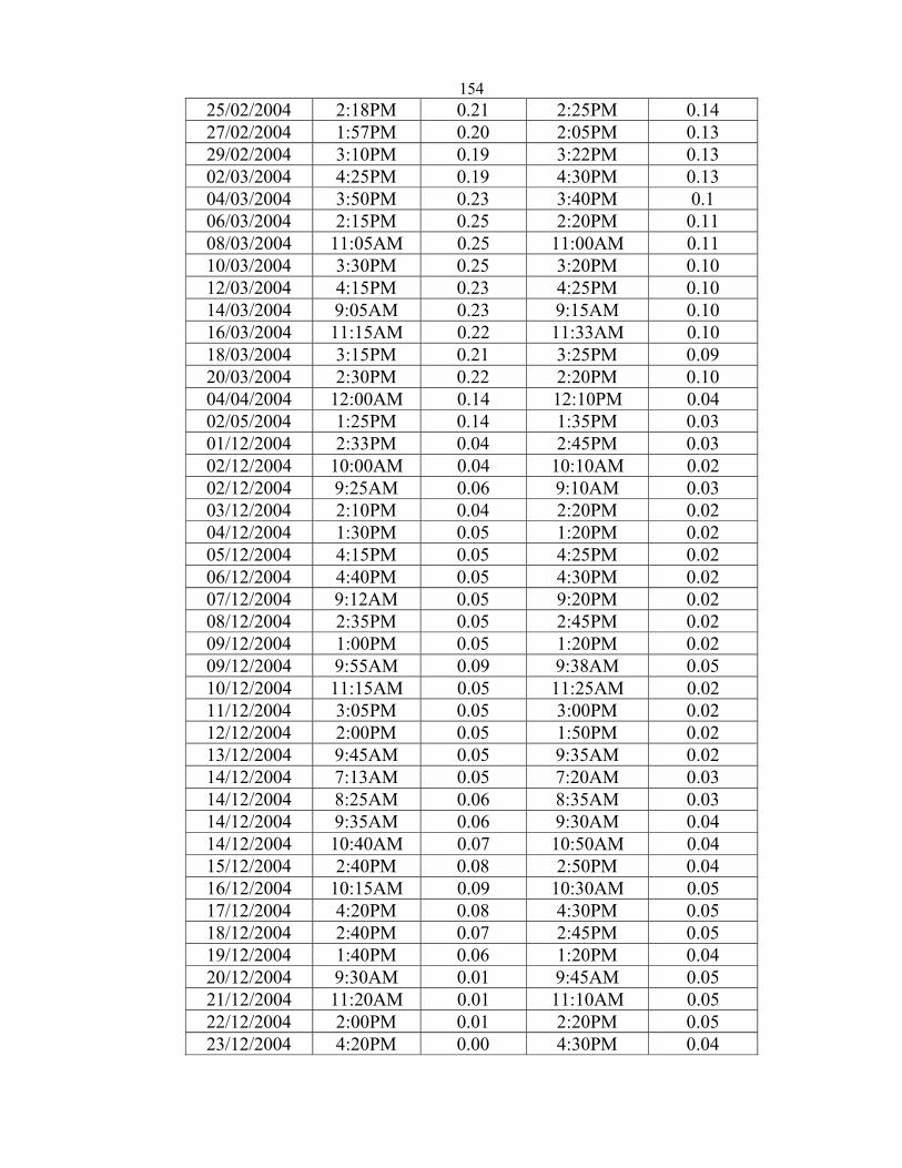
15425/02/2004 2:18PM 0.21 2:25PM 0.14 27/02/2004 1:57PM 0.20 2:05PM 0.13 29/02/2004 3:10PM 0.19 3:22PM 0.13 02/03/2004 4:25PM 0.19 4:30PM 0.13 04/03/2004 3:50PM 0.23 3:40PM 0.1 06/03/2004 2:15PM 0.25 2:20PM 0.11 08/03/2004 11:05AM 0.25 11:00AM 0.11 10/03/2004 3:30PM 0.25 3:20PM 0.10 12/03/2004 4:15PM 0.23 4:25PM 0.10 14/03/2004 9:05AM 0.23 9:15AM 0.10 16/03/2004 11:15AM 0.22 11:33AM 0.10 18/03/2004 3:15PM 0.21 3:25PM 0.09 20/03/2004 2:30PM 0.22 2:20PM 0.10 04/04/2004 12:00AM 0.14 12:10PM 0.04 02/05/2004 1:25PM 0.14 1:35PM 0.03 01/12/2004 2:33PM 0.04 2:45PM 0.03 02/12/2004 10:00AM 0.04 10:10AM 0.02 02/12/2004 9:25AM 0.06 9:10AM 0.03 03/12/2004 2:10PM 0.04 2:20PM 0.02 04/12/2004 1:30PM 0.05 1:20PM 0.02 05/12/2004 4:15PM 0.05 4:25PM 0.02 06/12/2004 4:40PM 0.05 4:30PM 0.02 07/12/2004 9:12AM 0.05 9:20PM 0.02 08/12/2004 2:35PM 0.05 2:45PM 0.02 09/12/2004 1:00PM 0.05 1:20PM 0.02 09/12/2004 9:55AM 0.09 9:38AM 0.05 10/12/2004 11:15AM 0.05 11:25AM 0.02 11/12/2004 3:05PM 0.05 3:00PM 0.02 12/12/2004 2:00PM 0.05 1:50PM 0.02 13/12/2004 9:45AM 0.05 9:35AM 0.02 14/12/2004 7:13AM 0.05 7:20AM 0.03 14/12/2004 8:25AM 0.06 8:35AM 0.03 14/12/2004 9:35AM 0.06 9:30AM 0.04 14/12/2004 10:40AM 0.07 10:50AM 0.04 15/12/2004 2:40PM 0.08 2:50PM 0.04 16/12/2004 10:15AM 0.09 10:30AM 0.05 17/12/2004 4:20PM 0.08 4:30PM 0.05 18/12/2004 2:40PM 0.07 2:45PM 0.05 19/12/2004 1:40PM 0.06 1:20PM 0.04 20/12/2004 9:30AM 0.01 9:45AM 0.05 21/12/2004 11:20AM 0.01 11:10AM 0.05 22/12/2004 2:00PM 0.01 2:20PM 0.05 23/12/2004 4:20PM 0.00 4:30PM 0.04
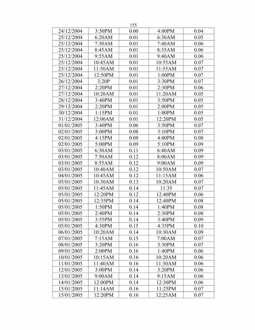
15524/12/2004 3:50PM 0.00 4:00PM 0.04 25/12/2004 6:20AM 0.01 6:30AM 0.05 25/12/2004 7:30AM 0.01 7:40AM 0.06 25/12/2004 8:45AM 0.01 8:35AM 0.06 25/12/2004 9:55AM 0.01 9:40AM 0.06 25/12/2004 10:45AM 0.01 10:55AM 0.07 25/12/2004 11:50AM 0.01 11:55AM 0.07 25/12/2004 12:50PM 0.01 1:00PM 0.07 26/12/2004 3:20P 0.01 3:30PM 0.07 27/12/2004 2:20PM 0.01 2:30PM 0.06 27/12/2004 10:20AM 0.01 11:20AM 0.05 28/12/2004 3:40PM 0.01 3:50PM 0.05 29/12/2004 2:20PM 0.01 2:00PM 0.05 30/12/2004 1:15PM 0.01 1:00PM 0.05 31/12/2004 12:00AM 0.01 12:20PM 0.05 01/01/2005 3:40PM 0.06 3:50PM 0.07 02/01/2005 3:00PM 0.08 3:10PM 0.07 02/01/2005 4:15PM 0.08 4:00PM 0.08 02/01/2005 5:00PM 0.09 5:10PM 0.09 03/01/2005 6:30AM 0.11 6:40AM 0.09 03/01/2005 7:50AM 0.12 8:00AM 0.09 03/01/2005 8:55AM 0.12 9:00AM 0.09 03/01/2005 10:40AM 0.12 10:50AM 0.07 04/01/2005 10:45AM 0.12 11:15AM 0.06 05/01/2005 10:30AM 0.13 10:20AM 0.07 05/01/2005 11:45AM 0.14 11:35 0.07 05/01/2005 12:20PM 0.12 12:40PM 0.06 05/01/2005 12:35PM 0.14 12:40PM 0.08 05/01/2005 1:50PM 0.14 1:40PM 0.08 05/01/2005 2:40PM 0.14 2:30PM 0.08 05/01/2005 3:55PM 0.14 3:40PM 0.09 05/01/2005 4:30PM 0.15 4:35PM 0.10 06/01/2005 10:20AM 0.14 10:30AM 0.09 07/01/2005 7:15AM 0.15 7:00AM 0.07 08/01/2005 3:20PM 0.16 3:30PM 0.07 09/01/2005 2:00PM 0.16 1:40PM 0.06 10/01/2005 10:15AM 0.16 10:20AM 0.06 11/01/2005 11:40AM 0.16 11:30AM 0.06 12/01/2005 3:00PM 0.14 3:20PM 0.06 13/01/2005 9:00AM 0.14 9:15AM 0.06 14/01/2005 12:00PM 0.14 12:30PM 0.06 15/01/2005 11:14AM 0.16 11:25PM 0.07 15/01/2005 12:20PM 0.16 12:25AM 0.07
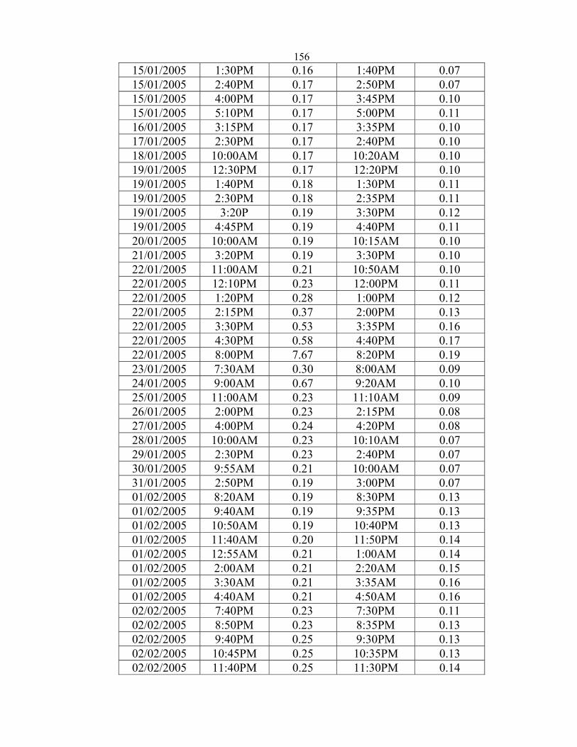
15615/01/2005 1:30PM 0.16 1:40PM 0.07 15/01/2005 2:40PM 0.17 2:50PM 0.07 15/01/2005 4:00PM 0.17 3:45PM 0.10 15/01/2005 5:10PM 0.17 5:00PM 0.11 16/01/2005 3:15PM 0.17 3:35PM 0.10 17/01/2005 2:30PM 0.17 2:40PM 0.10 18/01/2005 10:00AM 0.17 10:20AM 0.10 19/01/2005 12:30PM 0.17 12:20PM 0.10 19/01/2005 1:40PM 0.18 1:30PM 0.11 19/01/2005 2:30PM 0.18 2:35PM 0.11 19/01/2005 3:20P 0.19 3:30PM 0.12 19/01/2005 4:45PM 0.19 4:40PM 0.11 20/01/2005 10:00AM 0.19 10:15AM 0.10 21/01/2005 3:20PM 0.19 3:30PM 0.10 22/01/2005 11:00AM 0.21 10:50AM 0.10 22/01/2005 12:10PM 0.23 12:00PM 0.11 22/01/2005 1:20PM 0.28 1:00PM 0.12 22/01/2005 2:15PM 0.37 2:00PM 0.13 22/01/2005 3:30PM 0.53 3:35PM 0.16 22/01/2005 4:30PM 0.58 4:40PM 0.17 22/01/2005 8:00PM 7.67 8:20PM 0.19 23/01/2005 7:30AM 0.30 8:00AM 0.09 24/01/2005 9:00AM 0.67 9:20AM 0.10 25/01/2005 11:00AM 0.23 11:10AM 0.09 26/01/2005 2:00PM 0.23 2:15PM 0.08 27/01/2005 4:00PM 0.24 4:20PM 0.08 28/01/2005 10:00AM 0.23 10:10AM 0.07 29/01/2005 2:30PM 0.23 2:40PM 0.07 30/01/2005 9:55AM 0.21 10:00AM 0.07 31/01/2005 2:50PM 0.19 3:00PM 0.07 01/02/2005 8:20AM 0.19 8:30PM 0.13 01/02/2005 9:40AM 0.19 9:35PM 0.13 01/02/2005 10:50AM 0.19 10:40PM 0.13 01/02/2005 11:40AM 0.20 11:50PM 0.14 01/02/2005 12:55AM 0.21 1:00AM 0.14 01/02/2005 2:00AM 0.21 2:20AM 0.15 01/02/2005 3:30AM 0.21 3:35AM 0.16 01/02/2005 4:40AM 0.21 4:50AM 0.16 02/02/2005 7:40PM 0.23 7:30PM 0.11 02/02/2005 8:50PM 0.23 8:35PM 0.13 02/02/2005 9:40PM 0.25 9:30PM 0.13 02/02/2005 10:45PM 0.25 10:35PM 0.13 02/02/2005 11:40PM 0.25 11:30PM 0.14
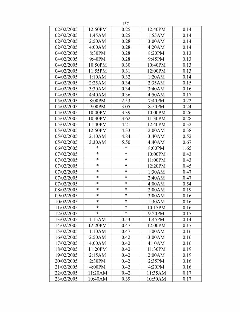
15702/02/2005 12:50PM 0.25 12:40PM 0.14 02/02/2005 1:45AM 0.25 1:55AM 0.14 02/02/2005 2:50AM 0.28 3:00AM 0.14 02/02/2005 4:00AM 0.28 4:20AM 0.14 04/02/2005 8:30PM 0.28 8:20PM 0.13 04/02/2005 9:40PM 0.28 9:45PM 0.13 04/02/2005 10:50PM 0.30 10:40PM 0.13 04/02/2005 11:55PM 0.31 12:00PM 0.13 04/02/2005 1:10AM 0.32 1:20AM 0.14 04/02/2005 2:25AM 0.34 2:35AM 0.15 04/02/2005 3:30AM 0.34 3:40AM 0.16 04/02/2005 4:40AM 0.36 4:50AM 0.17 05/02/2005 8:00PM 2.53 7:40PM 0.22 05/02/2005 9:00PM 3.05 8:50PM 0.24 05/02/2005 10:00PM 3.39 10:00PM 0.26 05/02/2005 10:30PM 3.62 11:30PM 0.28 05/02/2005 11:40PM 4.21 12:40PM 0.32 05/02/2005 12:50PM 4.33 2:00AM 0.38 05/02/2005 2:10AM 4.84 3:40AM 0.52 05/02/2005 3:30AM 5.50 4:40AM 0.67 06/02/2005 * * 8:00PM 1.65 07/02/2005 * * 10:00PM 0.43 07/02/2005 * * 11:00PM 0.43 07/02/2005 * * 12:20PM 0.45 07/02/2005 * * 1:30AM 0.47 07/02/2005 * * 2:40AM 0.47 07/02/2005 * * 4:00AM 0.54 08/02/2005 * * 2:00AM 0.19 09/02/2005 * * 3:00AM 0.16 10/02/2005 * * 1:30AM 0.16 11/02/2005 * * 10:15PM 0.16 12/02/2005 * * 9:20PM 0.17 13/02/2005 1:15AM 0.53 1:45PM 0.14 14/02/2005 12:20PM 0.47 12:00PM 0.17 15/02/2005 1:10AM 0.47 1:00AM 0.16 16/02/2005 2:50AM 0.42 3:00AM 0.16 17/02/2005 4:00AM 0.42 4:10AM 0.16 18/02/2005 11:20PM 0.42 11:30PM 0.19 19/02/2005 2:15AM 0.42 2:00AM 0.19 20/02/2005 2:30PM 0.42 2:35PM 0.16 21/02/2005 4:00PM 0.42 4:20PM 0.16 22/02/2005 11:20AM 0.42 11:35AM 0.17 23/02/2005 10:40AM 0.39 10:50AM 0.17
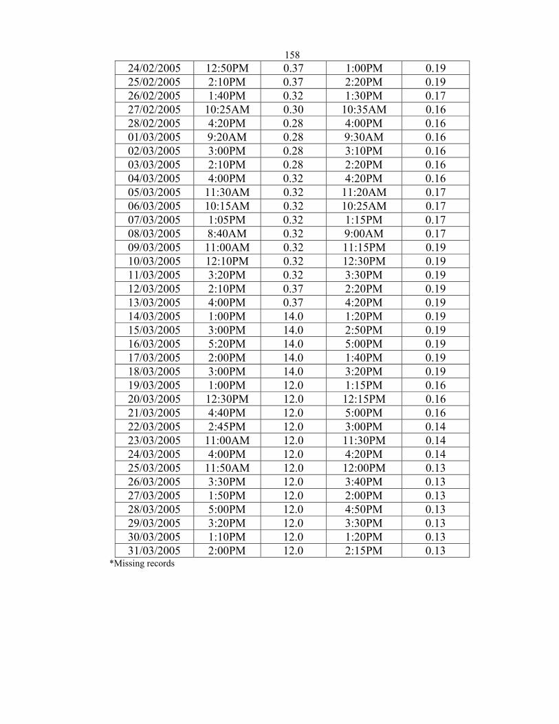
15824/02/2005 12:50PM 0.37 1:00PM 0.19 25/02/2005 2:10PM 0.37 2:20PM 0.19 26/02/2005 1:40PM 0.32 1:30PM 0.17 27/02/2005 10:25AM 0.30 10:35AM 0.16 28/02/2005 4:20PM 0.28 4:00PM 0.16 01/03/2005 9:20AM 0.28 9:30AM 0.16 02/03/2005 3:00PM 0.28 3:10PM 0.16 03/03/2005 2:10PM 0.28 2:20PM 0.16 04/03/2005 4:00PM 0.32 4:20PM 0.16 05/03/2005 11:30AM 0.32 11:20AM 0.17 06/03/2005 10:15AM 0.32 10:25AM 0.17 07/03/2005 1:05PM 0.32 1:15PM 0.17 08/03/2005 8:40AM 0.32 9:00AM 0.17 09/03/2005 11:00AM 0.32 11:15PM 0.19 10/03/2005 12:10PM 0.32 12:30PM 0.19 11/03/2005 3:20PM 0.32 3:30PM 0.19 12/03/2005 2:10PM 0.37 2:20PM 0.19 13/03/2005 4:00PM 0.37 4:20PM 0.19 14/03/2005 1:00PM 14.0 1:20PM 0.19 15/03/2005 3:00PM 14.0 2:50PM 0.19 16/03/2005 5:20PM 14.0 5:00PM 0.19 17/03/2005 2:00PM 14.0 1:40PM 0.19 18/03/2005 3:00PM 14.0 3:20PM 0.19 19/03/2005 1:00PM 12.0 1:15PM 0.16 20/03/2005 12:30PM 12.0 12:15PM 0.16 21/03/2005 4:40PM 12.0 5:00PM 0.16 22/03/2005 2:45PM 12.0 3:00PM 0.14 23/03/2005 11:00AM 12.0 11:30PM 0.14 24/03/2005 4:00PM 12.0 4:20PM 0.14 25/03/2005 11:50AM 12.0 12:00PM 0.13 26/03/2005 3:30PM 12.0 3:40PM 0.13 27/03/2005 1:50PM 12.0 2:00PM 0.13 28/03/2005 5:00PM 12.0 4:50PM 0.13 29/03/2005 3:20PM 12.0 3:30PM 0.13 30/03/2005 1:10PM 12.0 1:20PM 0.13 31/03/2005 2:00PM 12.0 2:15PM 0.13
*Missing records
159
APPENDIX A6
ANNUAL RAINFALL FOR THE SIX STATIONS WITHIN THE FARIA CATCHMENT
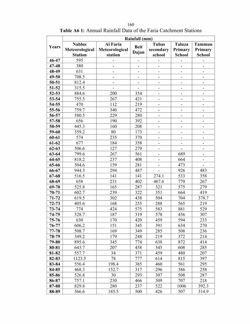
160Table A6 1: Annual Rainfall Data of the Faria Catchment Stations
Years
Rainfall (mm)Nablus
Meteorological Station
Al Faria Meteorological
station
Beit Dajan
Tubas secondary
school
Taluza Primary School
Tammun Primary School
46-47 595 - - - - - 47-48 380 - - - - - 48-49 631 - - - - - 49-50 708.5 - - - - - 50-51 812.4 - - - - - 51-52 315.5 - - - - - 52-53 884.6 200 354 - - - 53-54 755.5 267 421 - - - 54-55 470 112 219 - - - 55-56 759.7 340 472 - - - 56-57 580.5 229 280 - - - 57-58 656 190 392 - - - 58-59 445.3 160 208 - - - 59-60 359.2 80 173 - - - 60-61 574 235 370 - - - 61-62 677 184 358 - - - 62-63 506.6 127 279 - - - 63-64 799.6 267 561 - 689 - 64-65 818.2 237 408 - 664 - 65-66 504.6 159 281 - 473 - 66-67 944.3 294 487 - 926 483 67-68 516.5 141 141 274.1 533 358 68-69 658 231 402 467.6 770 267 69-70 525.8 165 287 321 575 279 70-71 602.7 239 322 351 664 419 71-72 619.5 302 438 504 704 378.7 72-73 405.6 168 255 288 565 219 73-74 774 424 575 583 881 529 74-75 528.7 187 319 378 456 307 75-76 630 170 420 459 594 233 76-77 606.2 151 345 391 634 270 77-78 508.7 169 349 285 508 236 78-79 349.2 179 248 219 372 214 79-80 895.6 345 774 638 872 414 80-81 643.7 207 458 345 608 285 81-82 557.7 34 371 459 480 207 82-83 1123.5 78 777 614 815 397 83-84 556.4 198.4 385 460 561 29584-85 468.3 152.7 317 296 386 258 85-86 526.8 30 293 307 508 287 86-87 757.1 230 466 309 707 218 87-88 829.8 280 237 522 1006 392.3 88-89 566.6 185.5 500 426 507 314.9
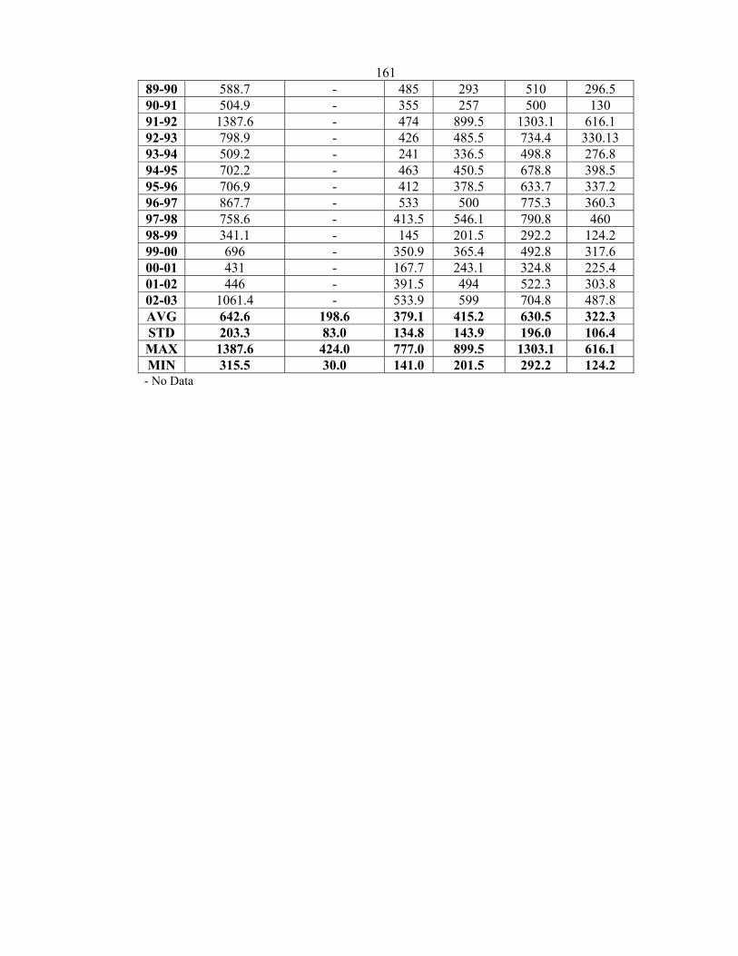
16189-90 588.7 - 485 293 510 296.5 90-91 504.9 - 355 257 500 130 91-92 1387.6 - 474 899.5 1303.1 616.1 92-93 798.9 - 426 485.5 734.4 330.13 93-94 509.2 - 241 336.5 498.8 276.8 94-95 702.2 - 463 450.5 678.8 398.5 95-96 706.9 - 412 378.5 633.7 337.2 96-97 867.7 - 533 500 775.3 360.3 97-98 758.6 - 413.5 546.1 790.8 46098-99 341.1 - 145 201.5 292.2 124.2 99-00 696 - 350.9 365.4 492.8 317.6 00-01 431 - 167.7 243.1 324.8 225.4 01-02 446 - 391.5 494 522.3 303.8 02-03 1061.4 - 533.9 599 704.8 487.8 AVG 642.6 198.6 379.1 415.2 630.5 322.3 STD 203.3 83.0 134.8 143.9 196.0 106.4 MAX 1387.6 424.0 777.0 899.5 1303.1 616.1 MIN 315.5 30.0 141.0 201.5 292.2 124.2
- No Data
162Appendix B (Figures)
Figure B1 1: Yearly Rainfall of Nablus Station ............................................. 164 Figure B1 2: Yearly Rainfall of Tubas Station ............................................... 164 Figure B1 3: Yearly Rainfall of Taluza Station ............................................. 165 Figure B1 4: Yearly Rainfall of Beit Dajan Station ....................................... 165 Figure B1 5: Yearly Rainfall of Tammun Station .......................................... 166 Figure B1 6: Yearly Rainfall of Al-Faria Station ........................................... 166 Figure B2 1: Gumbel Plots of Annual Rainfall of Nablus Station ................. 168 Figure B2 2: Gumbel Plots of Annual Rainfall of Taluza Station ................. 168 Figure B2 3: Gumbel Plots of Annual Rainfall of Tubas Station .................. 169 Figure B2 4: Gumbel Plots of Annual Rainfall of Beit Dajan Station ........... 169 Figure B2 5: Gumbel Plots of Annual Rainfall of Tammun Station .............. 170 Figure B2 6: Gumbel Plots of Annual Rainfall of Al-Faria Station .............. 170
163
APPENDIX B1
TIME SERIES PLOTS OF ANNUAL RAINFALL FOR THE STATIONS IN THE FARIA
CATCHMENT
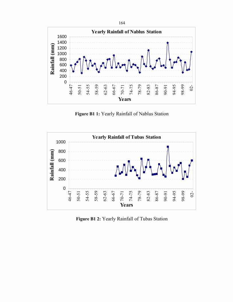
164
Yearly Rainfall of Nablus Station
0200400600800
1000120014001600
46-4
7
50-5
1
54-5
5
58-5
9
62-6
3
66-6
7
70-7
1
74-7
5
78-7
9
82-8
3
86-8
7
90-9
1
94-9
5
98-9
9
02-
Years
Rai
nfal
l (m
m)
Figure B1 1: Yearly Rainfall of Nablus Station
Yearly Rainfall of Tubas Station
0
200
400
600
800
1000
46-4
7
50-5
1
54-5
5
58-5
9
62-6
3
66-6
7
70-7
1
74-7
5
78-7
9
82-8
3
86-8
7
90-9
1
94-9
5
98-9
9
02-
Years
Rai
nfal
l (m
m)
Figure B1 2: Yearly Rainfall of Tubas Station

165
Yearly Rainfall of Taluza Station
0200400600800
100012001400
46-4
7
50-5
1
54-5
5
58-5
9
62-6
3
66-6
7
70-7
1
74-7
5
78-7
9
82-8
3
86-8
7
90-9
1
94-9
5
98-9
9
02-
Years
Rai
nfal
l (m
m)
Figure B1 3: Yearly Rainfall of Taluza Station
Yearly Rainfall of Beit Dajan Station
0
200
400
600
800
1000
46-4
7
50-5
1
54-5
5
58-5
9
62-6
3
66-6
7
70-7
1
74-7
5
78-7
9
82-8
3
86-8
7
90-9
1
94-9
5
98-9
9
02-
Years
Rai
nfal
l (m
m)
Figure B1 4: Yearly Rainfall of Beit Dajan Station
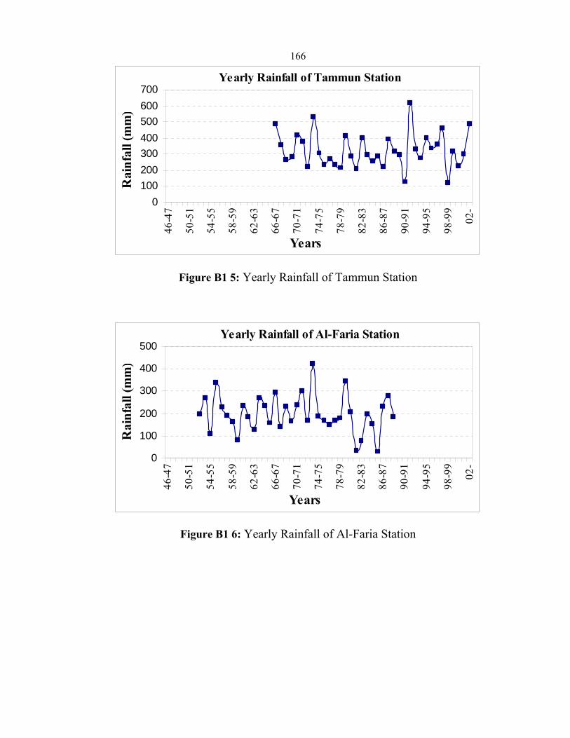
166
Yearly Rainfall of Tammun Station
0100200300400500600700
46-4
7
50-5
1
54-5
5
58-5
9
62-6
3
66-6
7
70-7
1
74-7
5
78-7
9
82-8
3
86-8
7
90-9
1
94-9
5
98-9
9
02-
Years
Rai
nfal
l (m
m)
Figure B1 5: Yearly Rainfall of Tammun Station
Yearly Rainfall of Al-Faria Station
0
100
200
300
400
500
46-4
7
50-5
1
54-5
5
58-5
9
62-6
3
66-6
7
70-7
1
74-7
5
78-7
9
82-8
3
86-8
7
90-9
1
94-9
5
98-9
9
02-
Years
Rai
nfal
l (m
m)
Figure B1 6: Yearly Rainfall of Al-Faria Station
167
APPENDIX B2
GUMBEL PLOTS OF ANNUAL RAINFALL FOR THE STATIONS IN THE FARIA CATCHMENT
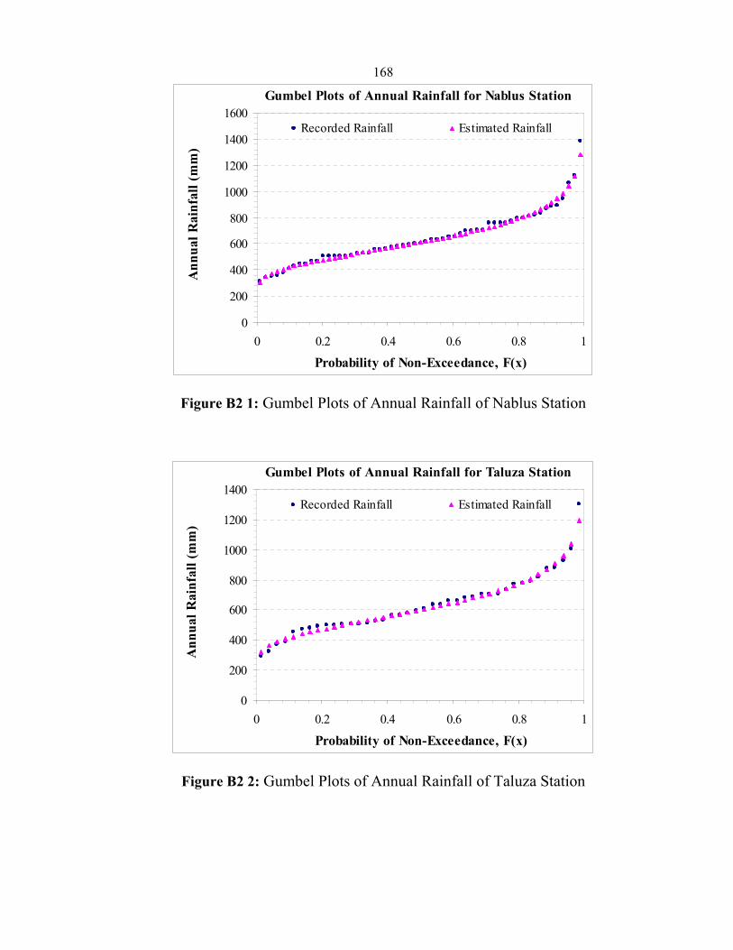
168
Gumbel Plots of Annual Rainfall for Nablus Station
0
200
400
600
800
1000
1200
1400
1600
0 0.2 0.4 0.6 0.8 1
Probability of Non-Exceedance, F(x)
Ann
ual R
ainf
all (
mm
)
Recorded Rainfall Estimated Rainfall
Figure B2 1: Gumbel Plots of Annual Rainfall of Nablus Station
Gumbel Plots of Annual Rainfall for Taluza Station
0
200
400
600
800
1000
1200
1400
0 0.2 0.4 0.6 0.8 1
Probability of Non-Exceedance, F(x)
Ann
ual R
ainf
all (
mm
)
Recorded Rainfall Estimated Rainfall
Figure B2 2: Gumbel Plots of Annual Rainfall of Taluza Station

169
Gumbel Plots of Annual Rainfall for Tubas Station
0
100200
300
400
500600
700
800900
1000
0 0.2 0.4 0.6 0.8 1
Probability of Non-Exceedance, F(x)
Ann
ual R
ainf
all (
mm
)
Recorded Rainfall Estimated Rainfall
Figure B2 3: Gumbel Plots of Annual Rainfall of Tubas Station
Gumbel Plots of Annual Rainfall for Beit Dajan Station
0
100
200
300
400
500
600
700
800
900
0 0.2 0.4 0.6 0.8 1
Probability of Non-Exceedance, F(x)
Ann
ual R
ainf
all (
mm
)
Recorded Rainfall Estimated Rainfall
Figure B2 4: Gumbel Plots of Annual Rainfall of Beit Dajan Station
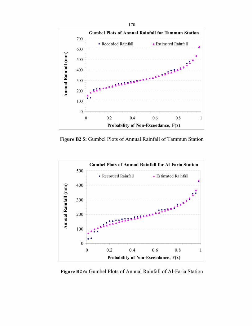
170
Gumbel Plots of Annual Rainfall for Tammun Station
0
100
200
300
400
500
600
700
0 0.2 0.4 0.6 0.8 1
Probability of Non-Exceedance, F(x)
Ann
ual R
ainf
all (
mm
)
Recorded Rainfall Estimated Rainfall
Figure B2 5: Gumbel Plots of Annual Rainfall of Tammun Station
Gumbel Plots of Annual Rainfall for Al-Faria Station
0
100
200
300
400
500
0 0.2 0.4 0.6 0.8 1Probability of Non-Exceedance, F(x)
Ann
ual R
ainf
all (
mm
)
Recorded Rainfall Estimated Rainfall
Figure B2 6: Gumbel Plots of Annual Rainfall of Al-Faria Station

171APPENDIX C (KW-GIUH Outputs)
Output C 1: KW-GIUH Results of 1-mm Excess Rainfall for Al-Badan Sub-catchment ...................................................................... 172
Output C 2: KW-GIUH Results of 1-mm Excess Rainfall for Al-Faria Sub-catchment.............................................................................. 174
Output C 3: KW-GIUH Results of 1-mm Excess Rainfall for Al-Badan Sub-catchment ...................................................................... 176
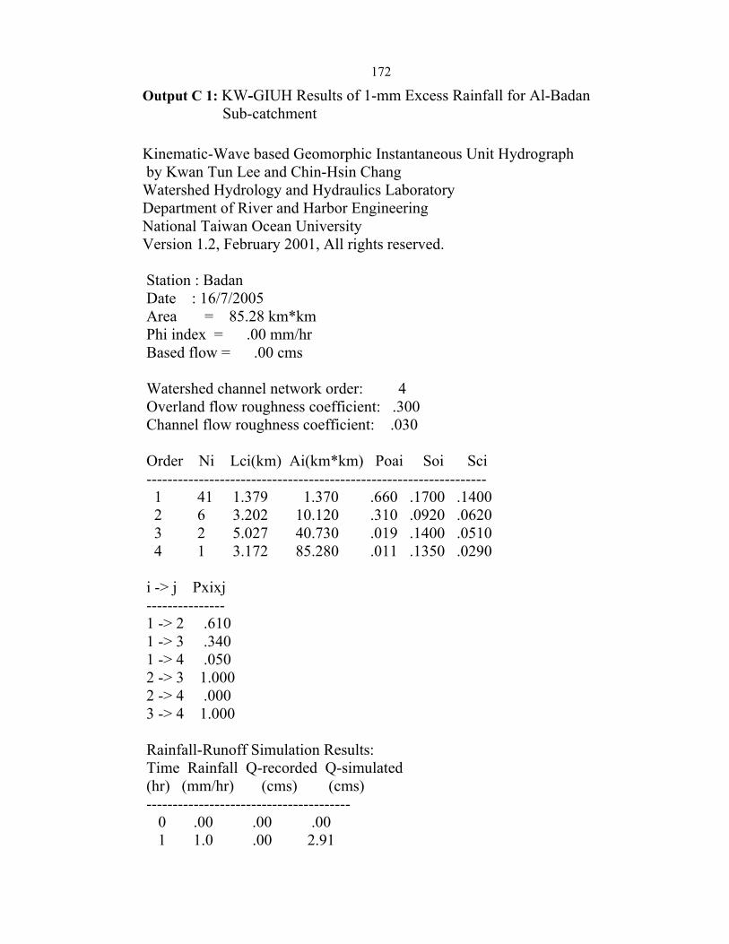
172
Output C 1: KW-GIUH Results of 1-mm Excess Rainfall for Al-Badan Sub-catchment
Kinematic-Wave based Geomorphic Instantaneous Unit Hydrograph by Kwan Tun Lee and Chin-Hsin Chang Watershed Hydrology and Hydraulics Laboratory Department of River and Harbor Engineering National Taiwan Ocean University Version 1.2, February 2001, All rights reserved. Station : Badan Date : 16/7/2005 Area = 85.28 km*km Phi index = .00 mm/hr Based flow = .00 cms Watershed channel network order: 4 Overland flow roughness coefficient: .300 Channel flow roughness coefficient: .030 Order Ni Lci(km) Ai(km*km) Poai Soi Sci ----------------------------------------------------------------- 1 41 1.379 1.370 .660 .1700 .1400 2 6 3.202 10.120 .310 .0920 .0620 3 2 5.027 40.730 .019 .1400 .0510 4 1 3.172 85.280 .011 .1350 .0290 i -> j Pxixj --------------- 1 -> 2 .610 1 -> 3 .340 1 -> 4 .050 2 -> 3 1.000 2 -> 4 .000 3 -> 4 1.000 Rainfall-Runoff Simulation Results: Time Rainfall Q-recorded Q-simulated (hr) (mm/hr) (cms) (cms) --------------------------------------- 0 .00 .00 .00 1 1.0 .00 2.91
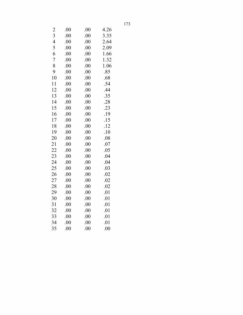
173 2 .00 .00 4.26 3 .00 .00 3.35 4 .00 .00 2.64 5 .00 .00 2.09 6 .00 .00 1.66 7 .00 .00 1.32 8 .00 .00 1.06 9 .00 .00 .85 10 .00 .00 .68 11 .00 .00 .54 12 .00 .00 .44 13 .00 .00 .35 14 .00 .00 .28 15 .00 .00 .23 16 .00 .00 .19 17 .00 .00 .15 18 .00 .00 .12 19 .00 .00 .10 20 .00 .00 .08 21 .00 .00 .07 22 .00 .00 .05 23 .00 .00 .04 24 .00 .00 .04 25 .00 .00 .03 26 .00 .00 .02 27 .00 .00 .02 28 .00 .00 .02 29 .00 .00 .01 30 .00 .00 .01 31 .00 .00 .01 32 .00 .00 .01 33 .00 .00 .01 34 .00 .00 .01 35 .00 .00 .00
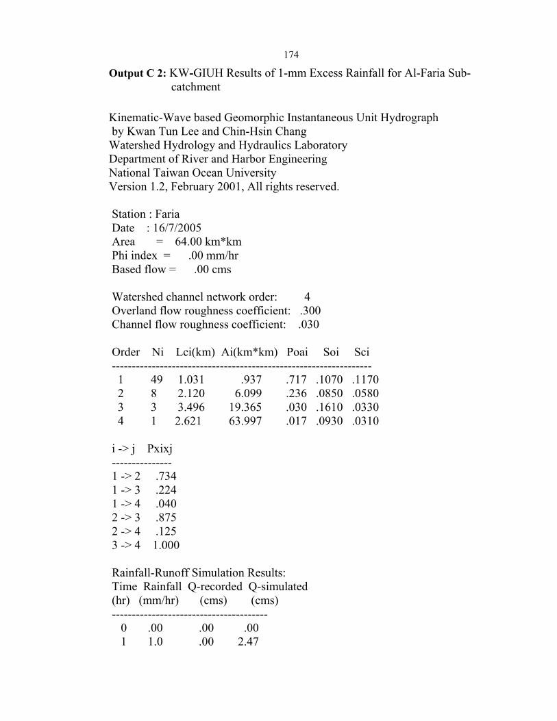
174
Output C 2: KW-GIUH Results of 1-mm Excess Rainfall for Al-Faria Sub-catchment
Kinematic-Wave based Geomorphic Instantaneous Unit Hydrograph by Kwan Tun Lee and Chin-Hsin Chang Watershed Hydrology and Hydraulics Laboratory Department of River and Harbor Engineering National Taiwan Ocean University Version 1.2, February 2001, All rights reserved. Station : Faria Date : 16/7/2005 Area = 64.00 km*km Phi index = .00 mm/hr Based flow = .00 cms Watershed channel network order: 4 Overland flow roughness coefficient: .300 Channel flow roughness coefficient: .030 Order Ni Lci(km) Ai(km*km) Poai Soi Sci ----------------------------------------------------------------- 1 49 1.031 .937 .717 .1070 .1170 2 8 2.120 6.099 .236 .0850 .0580 3 3 3.496 19.365 .030 .1610 .0330 4 1 2.621 63.997 .017 .0930 .0310 i -> j Pxixj --------------- 1 -> 2 .734 1 -> 3 .224 1 -> 4 .040 2 -> 3 .875 2 -> 4 .125 3 -> 4 1.000 Rainfall-Runoff Simulation Results: Time Rainfall Q-recorded Q-simulated (hr) (mm/hr) (cms) (cms) --------------------------------------- 0 .00 .00 .00 1 1.0 .00 2.47
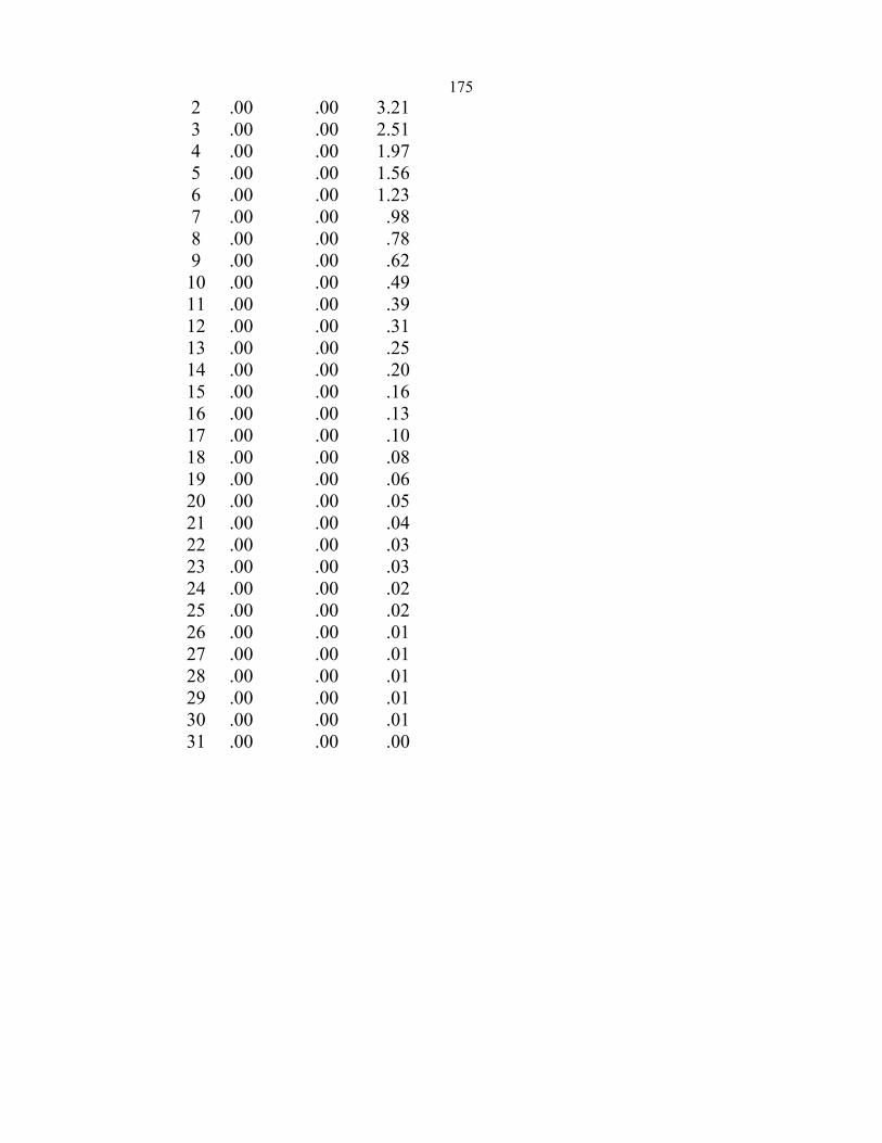
175 2 .00 .00 3.21 3 .00 .00 2.51 4 .00 .00 1.97 5 .00 .00 1.56 6 .00 .00 1.23 7 .00 .00 .98 8 .00 .00 .78 9 .00 .00 .62 10 .00 .00 .49 11 .00 .00 .39 12 .00 .00 .31 13 .00 .00 .25 14 .00 .00 .20 15 .00 .00 .16 16 .00 .00 .13 17 .00 .00 .10 18 .00 .00 .08 19 .00 .00 .06 20 .00 .00 .05 21 .00 .00 .04 22 .00 .00 .03 23 .00 .00 .03 24 .00 .00 .02 25 .00 .00 .02 26 .00 .00 .01 27 .00 .00 .01 28 .00 .00 .01 29 .00 .00 .01 30 .00 .00 .01 31 .00 .00 .00
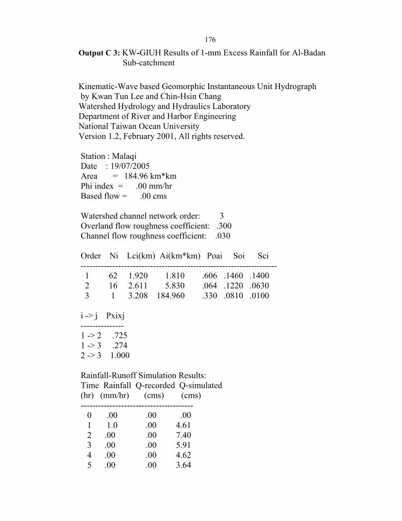
176
Output C 3: KW-GIUH Results of 1-mm Excess Rainfall for Al-Badan Sub-catchment
Kinematic-Wave based Geomorphic Instantaneous Unit Hydrograph by Kwan Tun Lee and Chin-Hsin Chang Watershed Hydrology and Hydraulics Laboratory Department of River and Harbor Engineering National Taiwan Ocean University Version 1.2, February 2001, All rights reserved. Station : Malaqi Date : 19/07/2005 Area = 184.96 km*km Phi index = .00 mm/hr Based flow = .00 cms Watershed channel network order: 3 Overland flow roughness coefficient: .300 Channel flow roughness coefficient: .030 Order Ni Lci(km) Ai(km*km) Poai Soi Sci -------------------------------------------------------------------- 1 62 1.920 1.810 .606 .1460 .1400 2 16 2.611 5.830 .064 .1220 .0630 3 1 3.208 184.960 .330 .0810 .0100 i -> j Pxixj --------------- 1 -> 2 .725 1 -> 3 .274 2 -> 3 1.000 Rainfall-Runoff Simulation Results: Time Rainfall Q-recorded Q-simulated (hr) (mm/hr) (cms) (cms) --------------------------------------- 0 .00 .00 .00 1 1.0 .00 4.61 2 .00 .00 7.40 3 .00 .00 5.91 4 .00 .00 4.62 5 .00 .00 3.64
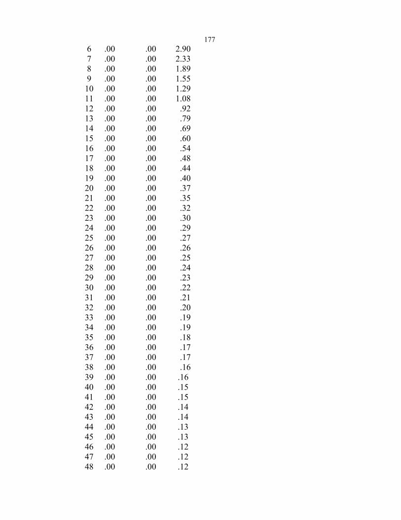
177 6 .00 .00 2.90 7 .00 .00 2.33 8 .00 .00 1.89 9 .00 .00 1.55 10 .00 .00 1.29 11 .00 .00 1.08 12 .00 .00 .92 13 .00 .00 .79 14 .00 .00 .69 15 .00 .00 .60 16 .00 .00 .54 17 .00 .00 .48 18 .00 .00 .44 19 .00 .00 .40 20 .00 .00 .37 21 .00 .00 .35 22 .00 .00 .32 23 .00 .00 .30 24 .00 .00 .29 25 .00 .00 .27 26 .00 .00 .26 27 .00 .00 .25 28 .00 .00 .24 29 .00 .00 .23 30 .00 .00 .22 31 .00 .00 .21 32 .00 .00 .20 33 .00 .00 .19 34 .00 .00 .19 35 .00 .00 .18 36 .00 .00 .17 37 .00 .00 .17 38 .00 .00 .16 39 .00 .00 .16 40 .00 .00 .15 41 .00 .00 .15 42 .00 .00 .14 43 .00 .00 .14 44 .00 .00 .13 45 .00 .00 .13 46 .00 .00 .12 47 .00 .00 .12 48 .00 .00 .12
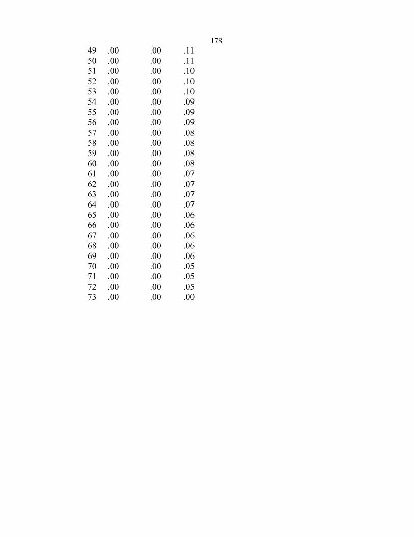
178 49 .00 .00 .11 50 .00 .00 .11 51 .00 .00 .10 52 .00 .00 .10 53 .00 .00 .10 54 .00 .00 .09 55 .00 .00 .09 56 .00 .00 .09 57 .00 .00 .08 58 .00 .00 .08 59 .00 .00 .08 60 .00 .00 .08 61 .00 .00 .07 62 .00 .00 .07 63 .00 .00 .07 64 .00 .00 .07 65 .00 .00 .06 66 .00 .00 .06 67 .00 .00 .06 68 .00 .00 .06 69 .00 .00 .06 70 .00 .00 .05 71 .00 .00 .05 72 .00 .00 .05 73 .00 .00 .00

179Appendix D (Pictures)
Picture D1 1: Al-Badan Flume .................................................................. 181 Picture D1 2: Al-Faria Flume .................................................................... 181 Picture D2 1: Al-Malaqi Bridge ................................................................ 183 Picture D2 2: Slope of Faria Catchment .................................................... 183 Picture D2 3: Up Stream of Al-Badan Sub-catchment ............................. 184 Picture D2 4: Agriculture in Faria Catchment .......................................... 184 Picture D2 5: Crop Fields in Faria Catchment .......................................... 185 Picture D2 6: Bare Land in Faria Catchment ............................................ 185
180
APPENDIX D1 PHOTOS OF AL-BADAN AND AL-FARIA
MEASURING FLUMES
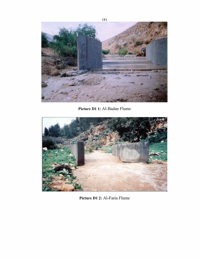
181
Picture D1 1: Al-Badan Flume
Picture D1 2: Al-Faria Flume

182
APPENDIX D2
FEATURES BY PHOTOS OF FARIA CATCHMENT
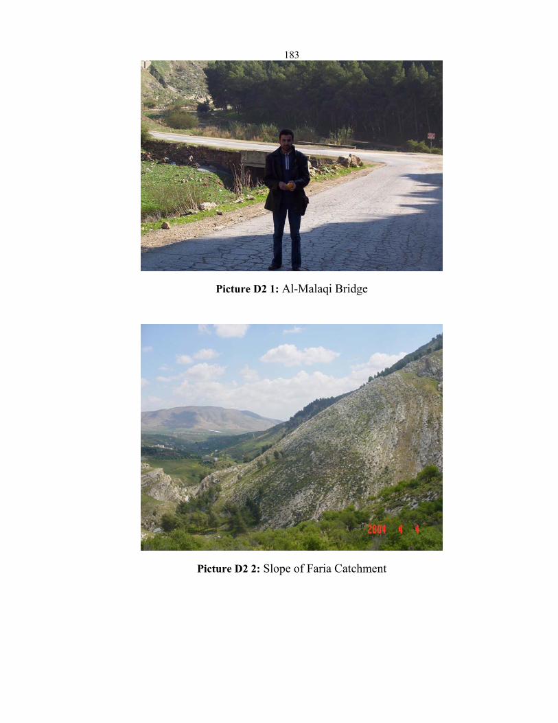
183
Picture D2 1: Al-Malaqi Bridge
Picture D2 2: Slope of Faria Catchment
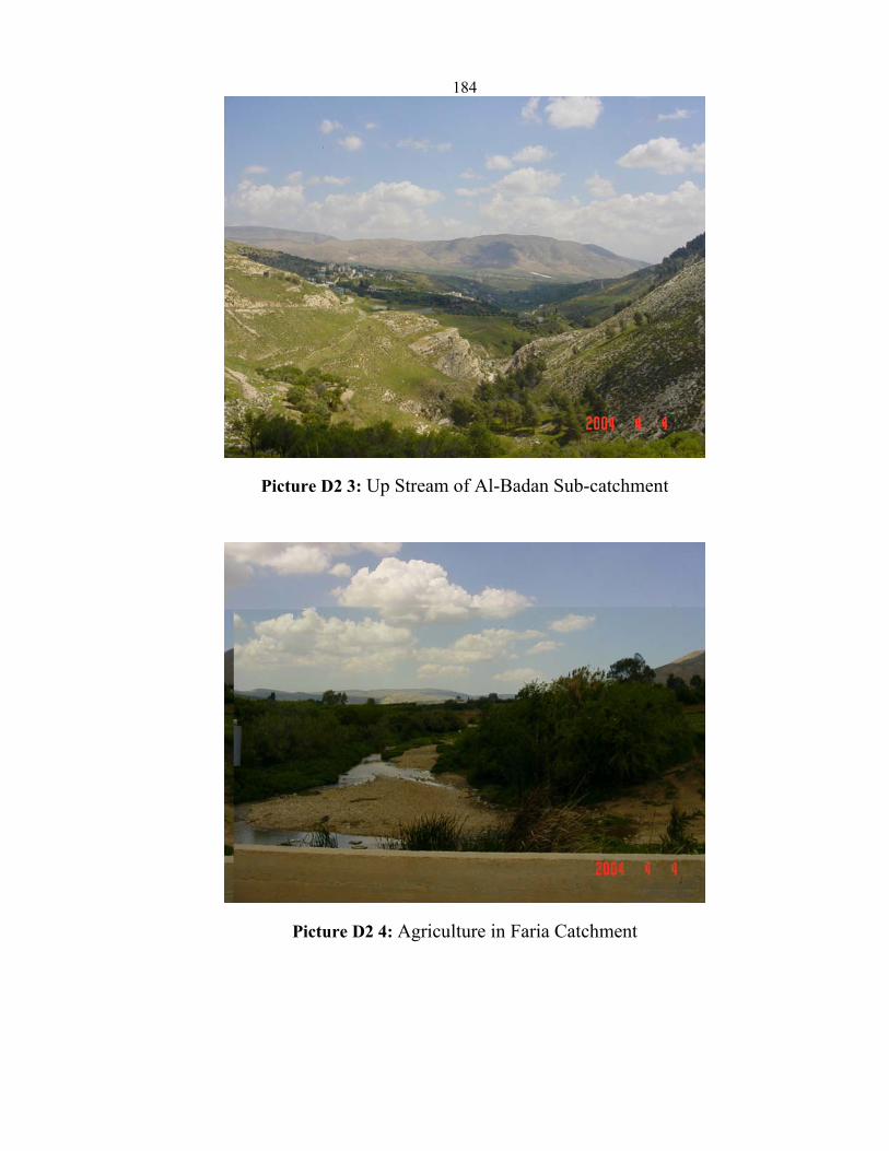
184
Picture D2 3: Up Stream of Al-Badan Sub-catchment
Picture D2 4: Agriculture in Faria Catchment
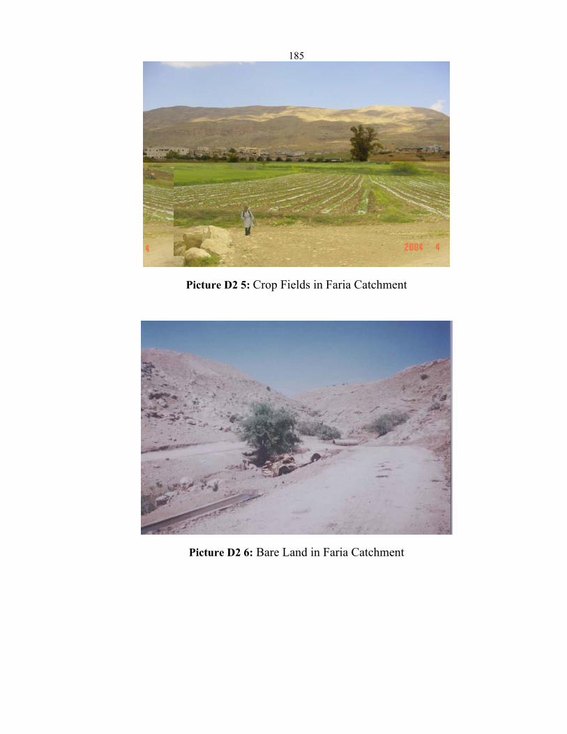
185
Picture D2 5: Crop Fields in Faria Catchment
Picture D2 6: Bare Land in Faria Catchment
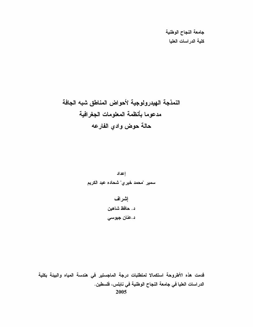
جامعة النجاح الوطنية
كلية الدراسات العليا
شبه الجافة لأحواض المناطقالنمذجة الهيدرولوجية
المعلومات الجغرافية بأنظمة مدعوما
عهوادي الفار حالة حوض
إعداد
عبد الكريمشحاده " محمد خيري"سمير
إشراف حافظ شاهين. د
عنان جيوسي.د
استكمالا لمتطلبات درجة الماجستير في هندسة المياه والبيئة بكلية الأطروحة قدمت هذه
.في جامعة النجاح الوطنية في نابلس، فلسطين الدراسات العليا2005

ب شبه الجافة لأحواض المناطقالنمذجة الهيدرولوجية
المعلومات الجغرافية مدعومة بأنظمة
وادي الفارعه حالة حوض
إعداد
عبد الكريمشحاده " د خيريمحم"سمير إشراف
حافظ شاهين. د
عنان جيوسي.د
الملخص
من ابرز الخصائص التي تميز النظام تعتبر العواصف الشديدة، الفيضانات والجفاف
والتي تعتبر من المناطق شبه الجافة، هناك عدد الضفة الغربيةفي . منطقة لأيالهيدرولوجي
).Hydrological Modeling(النمذجة الهيدرولوجية في مجالقليل من الدراسات المتوفرة
في هذه هي عبارة عن محاولة لدراسة ونمذجة العلاقة ما بين المطر والجريان رسالة الماجستير
يقع حوض وادي الفارعة في شمال شرق السفوح الشرقية . الحوض السطحي لوادي الفارعة
يوجد في . نطقة شبه جافةمنف على انه ويص 2كم334، حيث تبلغ مساحته حوالي للضفة الغربية
لجزء للمحطتين لقياس الجريان السطحي بالإضافة الأمطارست محطات لقياس هحوض الفارع
.لحوضمن ا العلوي
وهذا حوض وادي الفارعة محطاتجميع لأمطار إحصائيفي هذه الدراسة تم عمل تحليل
التوافق كذلك تم اختبار . مى والصغرىيتضمن المعدل السنوي، الانحراف المعياري والقيم العظ
Double( الكتليمنحنى الباستخدام طريقة )Internal Consistency( الأمطار لقياسات
Mass Curve( عد ذلك تم عمل تحليل للتوزيع قياسات المحطات متوافقة ب أنحيث وجد
يع توز أن حيث تبين السنوية لجميع المحطات في حوض الفارعة للأمطار الإحصائي
)Gumbel( يمكن الاعتماد على هذا التوزيع في الحسابات ويناسب البيانات المطرية السنوية
في حوض للأمطاروتقييم خصائص التوزيع الاحتمالي بما يمكن من فهم المستقبلية للمنطقة
.هالفارع
توجه هناك أنحيث كانت النتيجة السنوية مطارللأتوجه ال وتحليل ةدراستم أخرىمن ناحية
واضحاحيث كان هذا التوجه المناطق المرتفعة في )Increasing Trend(نحو الزيادة

ت
في Decreasing Trend)(بينما كان هناك توجه نجو النقصان لمحطتي نابلس وبيت دجن
لحوض الفارعه باستخدام الأمطارتم دراسة العلاقة بين محطات كذلك .المناطق المنخفضة
هناك علاقة قوية تربط تلك أنووجد Multiple Regression)(تعدد طريقة الانحسار الم
.المحطات
تم دراسة وتفحص العلاقة ما بين المطر والجريان السطحي لحوض وادي الرسالة في هذه
وهو منحنى KW-GIUH Model)(باستخدام النموذج الهيدرولوجي الذي يعرف باسم هالفارع
وذلك بالاستعانة ئص الجيومورفولوجية ومعادلة الحركةالتدفق الأحادي المعتمد على الخصا
تم اشتقاق منحنى التدفق النموذجوباستخدام هذا GIS)(ببرنامج نظم المعلومات الجغرافية
المشتقة تدل منحنيات التدفق . وادي الفارعه للأحواض الثلاثة التي يتشكل منها IUH)( الأحادي
لنمذجة الجريان السطحي في المناطق شبه للتطبيق هذا النموذج الهيدرولوجي قابل أنعلى
لأحواضلاستخدام وتوظيف هذا النموذج لاشتقاق منحنيات التدفق إمكانية وهذا يدل على الجافة
.السطحية في فلسطين