GIS and MATLAB modeling of criteria pollutants: a …...GIS and MATLAB modeling of pollutants, Nigeria 444 artificial neural network assemblage (ANN), for outdoor air quality. The

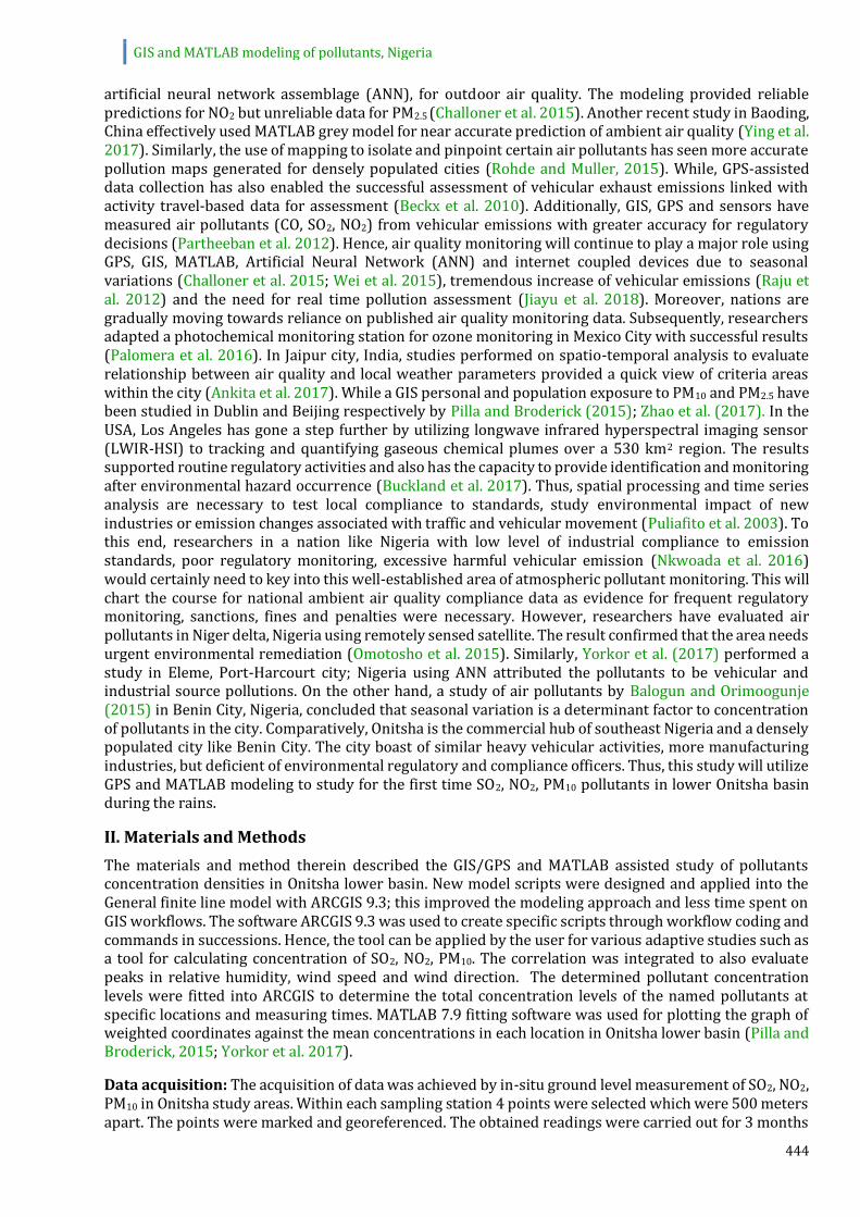
J. Sci. Technol. Environ. Inform. 06(01): 443-457 | Anyika et al. (2018) EISSN: 2409-7632, Journal home: www.journalbinet.com Crossref: https://doi.org/10.18801/jstei.060118.47

443 Published with open access at www.journalbinet.com

GIS and MATLAB modeling of criteria pollutants: a study of lower onitsha basin during rains Anyika L. C.1, Alisa, C. O.1, Nkwoada A. U.1, Opara A. I.2, Ejike E. N.1 and Onuoha G. N.1 1Dept. of Chemistry, Federal University of Technology Owerri, Nigeria 2Dept. of Geology, Federal University of Technology Owerri, Nigeria.

Article Information ABSTRACT

Key Words: Pollutants, Air quality, Model, Rains, Onitsha Nigeria Received: 10.06.2018 Revised: 19.09.2018 Published: 14 October 2018

For any information: [email protected]

The study of air pollutants SO2, NO2 and PM10 in lower Onitsha basin, a densely populated city was performed using GPS and Matlab modeling. The pollutants were studied in nine specific locations for 3 months of rains over 3 consecutive years with each georeferenced. The Matlab pollution model was generated by integrating the spatial database and measured pollution attributes database using a polynomial expression. SO2 highest concentration (141 µg/m3) peaked in Upper Iweka at sampling point 1 before dispersing to lower concentrated regions in Awada and Resthouse. NO2 peaked at 207 µg/m3 in Upper Iweka at sampling point 3 and driven by wind towards Borromeo area to very low concentration of 38 ug/m3. The PM10 peaked in Upper Iweka (180 µg/m3) and driven by rains towards Borromeo before increasing again in concentration levels at Awada. The AQI showed that SO2 pollutants had acceptable air quality at all sampling points while NO2 and PM10 air quality affected sensitive groups. SO2 concentration levels exceeded the National air quality standard in Nigeria (NAQS) while NO2 and PM10 were below the NAQS standard. The GIS plot showed that 3 metrological forces were driving pollutants from Upper Iweka and Awada to other sampling areas in the order of SO2> NO2> PM10. The Matlab wind speed plot showed that there was an upward wind in upper Iweka driving the pollutants towards dispersal at some other region. Thus, Upper Iweka is an active point source pollution area and dispersed to Borromeo and Awada by scavenging rains under prevailing wind speed, wind direction and humidity. Hence calls for improved monitoring and regulation to address pollution.

Citation: Anyika, L. C. Alisa, C. O. Nkwoada, A. U. Opara, A. I. Ejike, E. N. and Onuoha, G. N. (2018). GIS and MATLAB modeling of criteria pollutants: a study of lower onitsha basin during rains. Journal of Science, Technology and Environment Informatics, 06(01), 443-457. Crossref: https://doi.org/10.18801/jstei.060118.47

© 2018, Anyika et al. This is an open access article distributed under terms of the Creative Common Attribution 4.0 International License.

I. Introduction

Environmental pollution has remained a great concern to the nations of the world. Consequently, various techniques have been invented for monitoring air pollution using spatial processing and time series analysis (Ambare and Muhammed, 2013). For instance, NO2 and PM pollutants were studied using

Access by Smart Phone

https://doi.org/10.18801/jstei.060118.47

mailto:[email protected]


GIS and MATLAB modeling of pollutants, Nigeria

444

artificial neural network assemblage (ANN), for outdoor air quality. The modeling provided reliable predictions for NO2 but unreliable data for PM2.5 (Challoner et al. 2015). Another recent study in Baoding, China effectively used MATLAB grey model for near accurate prediction of ambient air quality (Ying et al. 2017). Similarly, the use of mapping to isolate and pinpoint certain air pollutants has seen more accurate pollution maps generated for densely populated cities (Rohde and Muller, 2015). While, GPS-assisted data collection has also enabled the successful assessment of vehicular exhaust emissions linked with activity travel-based data for assessment (Beckx et al. 2010). Additionally, GIS, GPS and sensors have measured air pollutants (CO, SO2, NO2) from vehicular emissions with greater accuracy for regulatory decisions (Partheeban et al. 2012). Hence, air quality monitoring will continue to play a major role using GPS, GIS, MATLAB, Artificial Neural Network (ANN) and internet coupled devices due to seasonal variations (Challoner et al. 2015; Wei et al. 2015), tremendous increase of vehicular emissions (Raju et al. 2012) and the need for real time pollution assessment (Jiayu et al. 2018). Moreover, nations are gradually moving towards reliance on published air quality monitoring data. Subsequently, researchers adapted a photochemical monitoring station for ozone monitoring in Mexico City with successful results (Palomera et al. 2016). In Jaipur city, India, studies performed on spatio-temporal analysis to evaluate relationship between air quality and local weather parameters provided a quick view of criteria areas within the city (Ankita et al. 2017). While a GIS personal and population exposure to PM10 and PM2.5 have been studied in Dublin and Beijing respectively by Pilla and Broderick (2015); Zhao et al. (2017). In the USA, Los Angeles has gone a step further by utilizing longwave infrared hyperspectral imaging sensor (LWIR-HSI) to tracking and quantifying gaseous chemical plumes over a 530 km2 region. The results supported routine regulatory activities and also has the capacity to provide identification and monitoring after environmental hazard occurrence (Buckland et al. 2017). Thus, spatial processing and time series analysis are necessary to test local compliance to standards, study environmental impact of new industries or emission changes associated with traffic and vehicular movement (Puliafito et al. 2003). To this end, researchers in a nation like Nigeria with low level of industrial compliance to emission standards, poor regulatory monitoring, excessive harmful vehicular emission (Nkwoada et al. 2016) would certainly need to key into this well-established area of atmospheric pollutant monitoring. This will chart the course for national ambient air quality compliance data as evidence for frequent regulatory monitoring, sanctions, fines and penalties were necessary. However, researchers have evaluated air pollutants in Niger delta, Nigeria using remotely sensed satellite. The result confirmed that the area needs urgent environmental remediation (Omotosho et al. 2015). Similarly, Yorkor et al. (2017) performed a study in Eleme, Port-Harcourt city; Nigeria using ANN attributed the pollutants to be vehicular and industrial source pollutions. On the other hand, a study of air pollutants by Balogun and Orimoogunje (2015) in Benin City, Nigeria, concluded that seasonal variation is a determinant factor to concentration of pollutants in the city. Comparatively, Onitsha is the commercial hub of southeast Nigeria and a densely populated city like Benin City. The city boast of similar heavy vehicular activities, more manufacturing industries, but deficient of environmental regulatory and compliance officers. Thus, this study will utilize GPS and MATLAB modeling to study for the first time SO2, NO2, PM10 pollutants in lower Onitsha basin during the rains.

II. Materials and Methods

The materials and method therein described the GIS/GPS and MATLAB assisted study of pollutants concentration densities in Onitsha lower basin. New model scripts were designed and applied into the General finite line model with ARCGIS 9.3; this improved the modeling approach and less time spent on GIS workflows. The software ARCGIS 9.3 was used to create specific scripts through workflow coding and commands in successions. Hence, the tool can be applied by the user for various adaptive studies such as a tool for calculating concentration of SO2, NO2, PM10. The correlation was integrated to also evaluate peaks in relative humidity, wind speed and wind direction. The determined pollutant concentration levels were fitted into ARCGIS to determine the total concentration levels of the named pollutants at specific locations and measuring times. MATLAB 7.9 fitting software was used for plotting the graph of weighted coordinates against the mean concentrations in each location in Onitsha lower basin (Pilla and Broderick, 2015; Yorkor et al. 2017).

Data acquisition: The acquisition of data was achieved by in-situ ground level measurement of SO2, NO2, PM10 in Onitsha study areas. Within each sampling station 4 points were selected which were 500 meters apart. The points were marked and georeferenced. The obtained readings were carried out for 3 months



with 72 hourly interval ranging from May 1st to July 1st which constitute rainy season peak period in Nigeria. Therefore, for the Onitsha study area with selected nine (9) sampling stations there are 6 x 9 experimental units. Experimental units mean six parameters to be tested x nine locations. Readings were taken at 3 months of rainy season which resulted to 54 experimental units. Each station has 4 points for sampling so that the Onitsha selected area has a total of two hundred and sixteen (216) determinations. Hence, in Onitsha there were obtained 1296 experimental units. This amounted to 5184 data for the rainy reason over a period of 3 years from 2013 to 2016 (Pilla and Broderick, 2015; Yorkor et al. 2017). A clear distribution of sampling locations was illustrated in Figure 01 (Google, 2018). Equipment and calibration: Gas and Particulate monitors was carried out using Crown on gas monitor Model CE 89/336/EEC obtained from the Imo State Environmental Protection Agency. The equipment was used for NO2, SO2 and PM10. PM10was monitored by switching to Crown on Particulate Monitor Model No. 1000 with serial no. 298621. The Wind speed and direction were determined as windrose using a digital meter. Relative humidity and temperature were determined with the same Environmental Meter Model AE.09605 by Rumsey Environmental LLC, from Mechanical Engineering Department; Federal University of Technology, Owerri which is located in the Weather/Erosion monitoring unit in the institution. The sensors were recalibrated and stabilized by exposure for several hours in a sealed vessel at room temperature prior to measurement. NO2 and SO2gas were used as applicable. NO2 gas concentrations ranging from 0-1000 ppb was used to recalibrate the SnO2 sensor connected to evaluation circuit board which records sensor responses. This calibration was repeated for SO2 gas sensor. The protocol for recalibration of particulate matter at PM10 to establish the sensitivity was applied and recorded. Recalibration of the monitors were done at Imo State Environmental Protection Agency (ISEPA) laboratories in Owerri using established and well reported methodologies Pilla and Broderick, 2015; Yorkor et al. 2017; GNI, 2007).

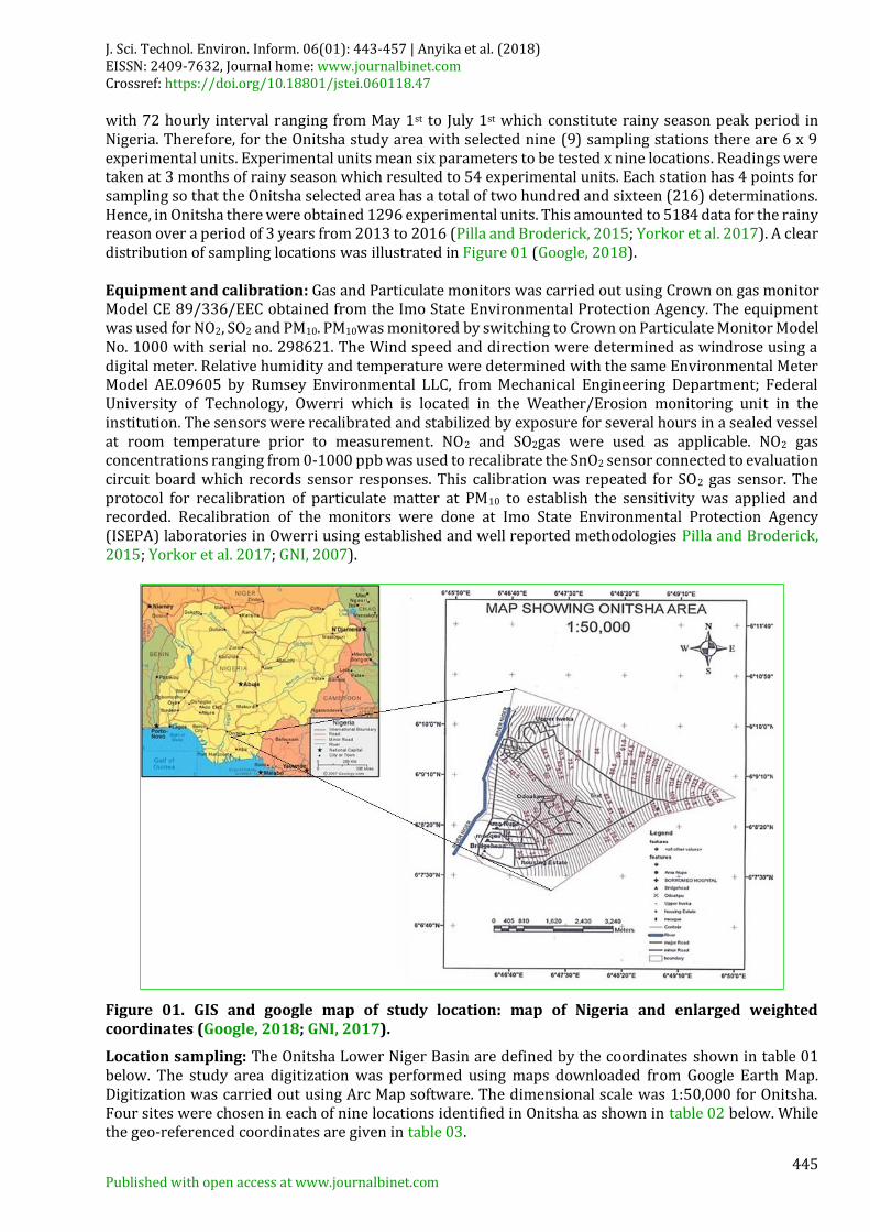
Figure 01. GIS and google map of study location: map of Nigeria and enlarged weighted coordinates (Google, 2018; GNI, 2017).

Location sampling: The Onitsha Lower Niger Basin are defined by the coordinates shown in table 01 below. The study area digitization was performed using maps downloaded from Google Earth Map. Digitization was carried out using Arc Map software. The dimensional scale was 1:50,000 for Onitsha. Four sites were chosen in each of nine locations identified in Onitsha as shown in table 02 below. While the geo-referenced coordinates are given in table 03.



446

Table 01. Onitsha latitude and longitude coordinates

N06o 07׀ E006o 47׀ N06o 08׀ E006o 46׀ N06o 09׀ E006o 47׀

N06o 07׀ E006o 48׀ N06o 08׀ E006o 47׀

Table 02. Nine locations of Onitsha study area

Upper Iweka/Nitel Port Harcourt road/Niger state Feggie/Nupe Square

Mission road/waterside Rest house/GRA Christ the king college (CKC)

Uzodinma street Borromeo hospital Araba/Oraifite street/Abs.Ch.27

Table 03. Georeferenced coordinates of sampling stations in rainy season in Onitsha

Sampling station

Co-ordinates

Point 1 Point 2 Point 3 Point 4

Upper iweka/nitel

NO60 07.851ʹ

E 0060 47.660ʹ

NO60 08.095ʹ

E 0060 47.447ʹ

NO60 08.062ʹ

E 0060 47.664ʹ

NO60 07.933ʹ

E 0060 47.470ʹ

Ph road/niger st.

NO60 08.023ʹ

E0060 47.405ʹ

NO60 08.001ʹ

E0060 16.124ʹ

NO60 07.918ʹ

E0060 46.098ʹ

NO60 08.090ʹ

E0060 46.125ʹ

Egge/nupe square

NO60 08.074ʹ

E0060 46.216ʹ

NO60 08.102ʹ

E0060 46.263ʹ

NO60 08.084ʹ

E0060 46.168ʹ

NO60 08.179ʹ

E0060 46.179ʹ

Uzodinma str. Fegge

NO60 08.271ʹ

E0060 46.395ʹ

NO60 08.212ʹ

E0060 46.399ʹ

NO60 08.212ʹ

E0060 46.520ʹ

NO60 08.263ʹ

E0060 46.522ʹ

Mission rd./waterside

NO60 09.567ʹ

E0060 46.762ʹ

NO60 09.634ʹ

E0060 46.511ʹ

NO60 09.780ʹ

E0060 46.583ʹ

NO60 09.709ʹ

E0060 46.773ʹ

Rest house/gra

NO60 09.685ʹ

E0060 47.019ʹ

NO60 09.700ʹ

E0060 47.044ʹ

NO60 09.766ʹ

E0060 47.038ʹ

NO60 09.744ʹ

E0060 47.032ʹ

C.k.c

NO60 08.609ʹ

E0060 47.469ʹ

NO60 08.550ʹ

E0060 47.494ʹ

NO60 08.481ʹ

E0060 47.341ʹ

NO60 08.535ʹ

E0060 47.244ʹ

Borromeo hospital

NO60 08.745ʹ

E0060 49.070ʹ

NO60 08.618ʹ

E0060 49.113ʹ

NO60 08.591ʹ

E0060 49.065ʹ

NO60 08.557ʹ

E0060 49.131ʹ

Awada/oraifite st./abs.

Channel 27

NO60 07.743ʹ

E0060 48.180ʹ

NO60 07.700ʹ

E0060 48.204ʹ

NO60 07.661ʹ

E0060 48.085ʹ

NO60 07.627ʹ

E0060 48.099ʹ

MATLAB assisted modeling: The pollution characteristics (model) of the study area was generated by integrating the spatial data base and measured pollution attributes data base using the polynomial expression (Raju et al. 2012; Jiayu et al. 2018; Palomera et al. 2016).

yj= k + k1x1 + k2x2 +k3x3 … +knxn

Where, yj represents the coordinates for points 1, 2, 3, 4, in each location which constitutes the spatial data base, the pollution index at any given sampling station can be represented by a function y which depends on the contributions of the various concentrations of the identified pollutants, the windrose and the meteorological conditions such as relative humidity, temperature etc. So that at a given sample station with four sampling points, four simultaneous equations can be written to represent the air pollution index at that station. where y1 = Pollution index at a given coordinate such as point 1, k is an empirical constant k1, k2, k3, are constants which modify the empirical pollutant concentrations and are the constants for the variables SO2, NO2 and PM10 respectively. The application of matrix algebra was used to solve the set of the simultaneous (Raju et al. 2012; Jiayu et al. 2018; Palomera et al. 2016; Park et al. 2013). Function results from solution to the simultaneous equations which imputes xi and yi values so that in MATLAB 7.9 Notation we can write:

𝐺 = 𝑖𝑛𝑌(𝑋) … … … … … … … . (1)

𝐾 = 𝐺 ∗ 𝑦𝑖 … … … … … … … … (2)



Where, G is the variable that outputs the inverse of the matrix X.

Air Quality Index (AQI): The air quality index (AQI) is an index system of number grading that indicates the level of pollution in the atmosphere. AQI determination is carried out by calculating the IAQI (Individual air quality index) for each pollutant. Where the formula is given below as

𝐼𝐴𝑄𝐼 = 𝐼𝐴𝑄𝐼𝐻𝐼− 𝐼𝐴𝑄𝐼𝐿𝑜

𝐵𝑃𝐻𝐼−𝐵𝑃𝐿𝑂(𝐶𝑝 − 𝐵𝑃𝐿𝑂) + 𝐼𝐴𝑄𝐼𝐿𝑂………………………. (3)

The IAQIP is the individual air quality index for pollutants P (PM10, SO2, NO2) and CP is the daily mean concentration of the pollutant P. BPLO and BPHI are the nearest and lowest values of Cp The IAQILO and IAQIHI are the individual air quality indexes in terms of BPHI and BPLO as shown in table 04. From the table 04, the IAQI maximum is 500. After the calculation of individual air quality index (IAQIP) for each pollutant, the AQI would then be determined by selecting the maximum IAQIP as follows:

𝐴𝑄𝐼 = max (𝐼𝐴𝑄𝐼1 , … . 𝐼𝐴𝑄𝐼𝑛)…………………………. (4)

Hence, the equation (4) demonstrates that AQI calculation is not the sum of all the pollutants involved but is the maximum value of IAQI obtained. Although NAAQS-2012, PM10, SO2, NO2 are included in the calculation, however, the air pollutant with a maximum IAQI when AQI is larger than 50 is then termed the principal pollutant. Whereas daily AQI less than 100 is supposed to be qualified using NAAQS-2012 (Wei et al. 2015; Park et al. 2013; Youping et al. 2018; Kanchan and Goyal, 2015).

Table 04. Air quality index (AQI) grading for pollutants

AQI

values

0-50 51-100 101-150 151-200 201-300 301-400 401-500

Levels of

health

concern

Good moderate Unhealthy for

sensitive

groups

Unhealthy Very

Unhealthy

Hazardous Hazardous

Colour

code

Green Yellow Orange Red Purple Maroon Maroon

Meaning Air quality is

considered

satisfactory

Air quality is

acceptable,

however, for some

pollutants there

may be a

moderate health

concern for a very

small number of

people who are

unusually

sensitive to air

pollution.

Members of

sensitive

groups may

experience

health effects.

The general

public is not

likely to be

affected.

Everyone may

begin to

experience

health effects:

members of

sensitive

groups may

experience

more serious

health effects.

Health alert:

everyone

may

experience

more serious

health

effects.

Health

warning of

emergency

conditions.

The entire

population is

more likely to

be affected.

Health

warning of

emergency

conditions.

The entire

population is

more likely to

be affected.

Adapted from: Environmental Protection Agency Durham, North Carolina USA (EPA, 2016).

III. Results and Discussion

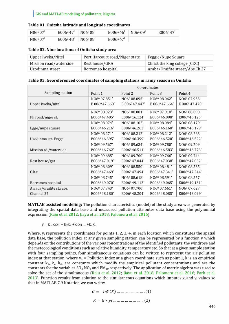
SO2 concentration The concentrations of the SO2 gas was plotted using the box and whiskers chat as seen in figure 02 below. The sampling point 1 of upper Iweka coordinates/region gave the highest concentrations of SO2gas at 141 µg/m3.This value almost doubled the concentration at other sampling points except CKC point 2and rest house point 3. The lowest recorded concentration of SO2 was point 1 and point 2 of Mission road and Borromeo hospital respectively. A closer observation shows that there appear to be more concentrations of CO2 at Fegge, Uzodinma, mission road before dispersing again from Resthouse to Awada. Thus, there may be a sloping region causing this pollutant undulation and dispersal. Another explanation could be that Fegge, Uzodinma and mission road could be point sources for SO2 emission and which eventually gets concentrated at other regions such as upper Iweka, CKC and Awada regions. on the average sampling point 1 showed the highest concentration levels of SO2 while sampling point 4 showed the lowest and point 5 was the average of the four sampling points.



448

Figure 02. Box and whiskers plot for SO2 concentration in Onitsha lower basin.

They result when compared to neighboring city of Aba as studied by Akuagwu et al. (2016) and Orlu as studied by Ibe et al. (2017) and showed that Onitsha lower basin was significantly polluted when compared to these cities. Also, the high concentration of SO2exceeded the study performed in selected areas of Lagos metropolis (Njoku et al. 2016).

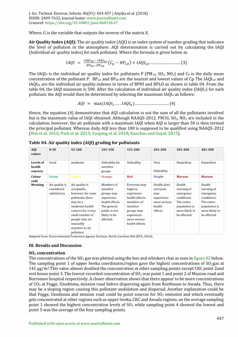
Figure 03. Box and whiskers plot for NO2 concentration in Onitsha lower basin during rainy season.

NO2 Concentration The box and whiskers plot for NO2 concentration is presented in figure 03 below showing the concentrations at various locations. The figure shows that Upper Iweka (point 3), had the highest concentration of NO2 gaseous pollutants (207 µg/m3) while the lowest was Borromeo at 38 µg/m3 (point 4). The appearance of the figure seems to connote a kind of undulating wind driving the NO2 molecules. These would have cause the molecules to experience dispersion at Upper Iweka and Awada. While aggregation is experienced at other sampling points. CKC and Borromeo experienced the lowest wind action, hence the highest level of aggregation. This idea is supported by the fact that at upper Iweka was high concentration of NO2 whose concentration will reduce as it travels within the wind. These molecules will eventually get dispersed to other regions at small concentration. However, on the converse, the CKC and Borromeo and PH road may be point source pollutions due to agglomeration and low wind action. However, such free molecules may now be displaced towards a region of less dispersive wind and eventually remains high at such regions such as Upper Iweka and Awada area. A similar form of pollutant



movement was observed in SO2 at Upper Iweka, mission road and Borromeo.Additionally, in both gases sampling point 4 were points of lowest concentration.

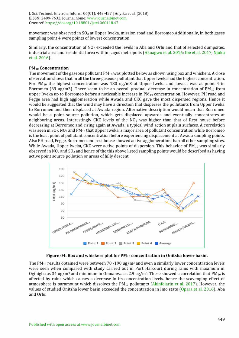
Similarly, the concentration of NO2 exceeded the levels in Aba and Orlu and that of selected dumpsites, industrial area and residential area within Lagos metropolis (Akuagwu et al. 2016; Ibe et al. 2017; Njoku et al. 2016). PM10 Concentration The movement of the gaseous pollutant PM10 was plotted below as shown using box and whiskers. A close observation shows that in all the three-gaseous pollutant that Upper Iweka had the highest concentration. For PM10 the highest concentration was 180 ug/m3 at Upper Iweka and lowest was at point 4 in Borromeo (69 ug/m3). There seem to be an overall gradual; decrease in concentration of PM10 from upper Iweka up to Borromeo before a noticeable increase in PM10 concentration. However, PH road and Fegge area had high agglomeration while Awada and CKC gave the most dispersed regions. Hence it would be suggested that the wind may have a direction that disperses the pollutants from Upper Iweka to Borromeo and then displaced at Awada region. Alternative description would mean that Borromeo would be a point source pollution, which gets displaced upwards and eventually concentrates at neighboring areas. Interestingly CKC levels of the NO2 was higher than that of Rest house before decreasing at Borromeo and rising again at Awada; a typical wind action at plain surfaces. A correlation was seen in SO2, NO2 and PM10 that Upper Iweka is major area of pollutant concentration while Borromeo is the least point of pollutant concentration before experiencing displacement at Awada sampling points. Also PH road, Fegge, Borromeo and rest house showed active agglomeration than all other sampling sites. While Awada, Upper Iweka, CKC were active points of dispersion. This behavior of PM10 was similarly observed in NO2 and SO2 and hence of the this above listed sampling points would be described as having active point source pollution or areas of hilly descent.

Figure 04. Box and whiskers plot for PM10 concentration in Onitsha lower basin.

The PM10 results obtained were between 70 -190 ug/m3 and even a similarly lower concentration levels were seen when compared with study carried out in Port Harcourt during rains with maximum in Oginigba as 34 ug/m3 and minimum in Omuanwa as 2.9 ug/m3. These showed a correlation that PM10 is affected by rains which causes a decrease in its concentration levels. hence the scavenging effect of atmosphere is paramount which dissolves the PM10 pollutants (Akinfolarin et al. 2017). However, the values of studied Onitsha lower basin exceeded the concentration in Imo state (Opara et al. 2016), Aba and Orlu.



450

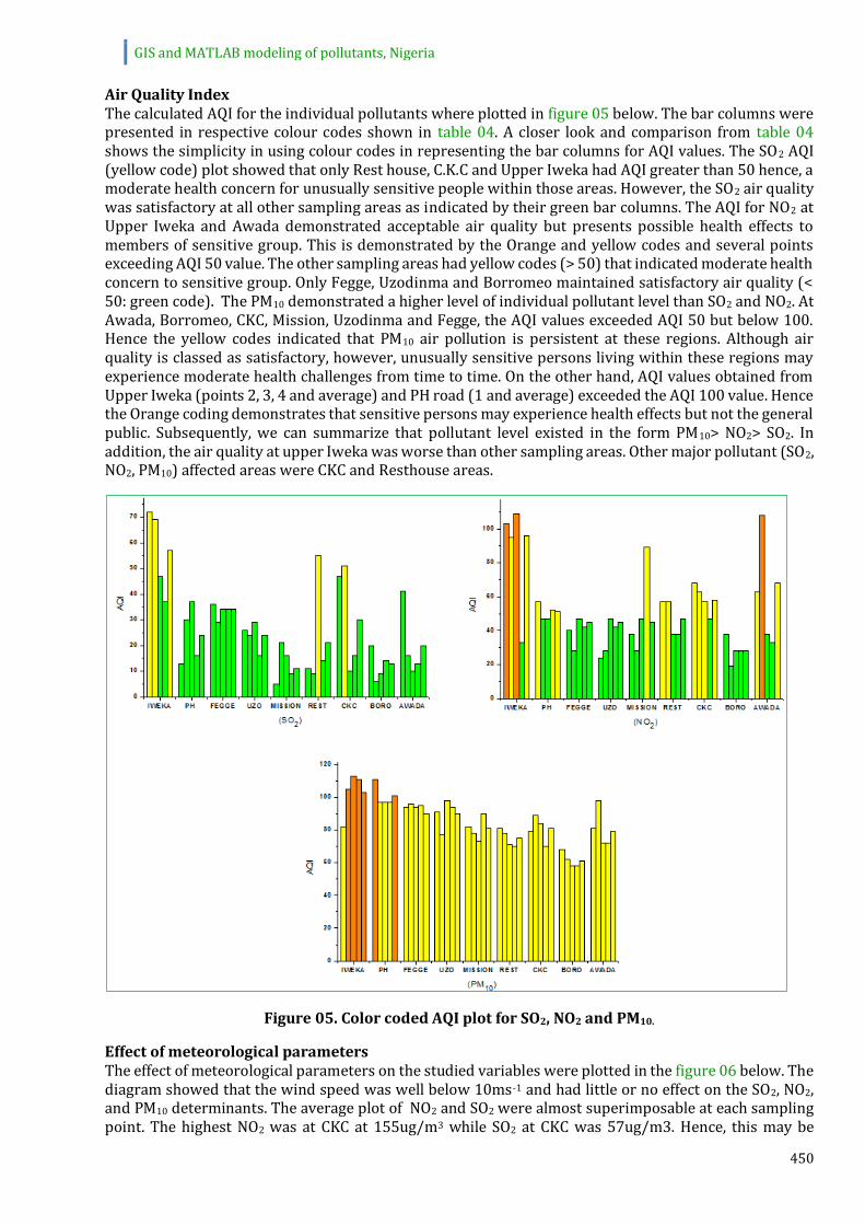
Air Quality Index The calculated AQI for the individual pollutants where plotted in figure 05 below. The bar columns were presented in respective colour codes shown in table 04. A closer look and comparison from table 04 shows the simplicity in using colour codes in representing the bar columns for AQI values. The SO2 AQI (yellow code) plot showed that only Rest house, C.K.C and Upper Iweka had AQI greater than 50 hence, a moderate health concern for unusually sensitive people within those areas. However, the SO2 air quality was satisfactory at all other sampling areas as indicated by their green bar columns. The AQI for NO2 at Upper Iweka and Awada demonstrated acceptable air quality but presents possible health effects to members of sensitive group. This is demonstrated by the Orange and yellow codes and several points exceeding AQI 50 value. The other sampling areas had yellow codes (> 50) that indicated moderate health concern to sensitive group. Only Fegge, Uzodinma and Borromeo maintained satisfactory air quality (< 50: green code). The PM10 demonstrated a higher level of individual pollutant level than SO2 and NO2. At Awada, Borromeo, CKC, Mission, Uzodinma and Fegge, the AQI values exceeded AQI 50 but below 100. Hence the yellow codes indicated that PM10 air pollution is persistent at these regions. Although air quality is classed as satisfactory, however, unusually sensitive persons living within these regions may experience moderate health challenges from time to time. On the other hand, AQI values obtained from Upper Iweka (points 2, 3, 4 and average) and PH road (1 and average) exceeded the AQI 100 value. Hence the Orange coding demonstrates that sensitive persons may experience health effects but not the general public. Subsequently, we can summarize that pollutant level existed in the form PM10> NO2> SO2. In addition, the air quality at upper Iweka was worse than other sampling areas. Other major pollutant (SO2, NO2, PM10) affected areas were CKC and Resthouse areas.

Figure 05. Color coded AQI plot for SO2, NO2 and PM10.

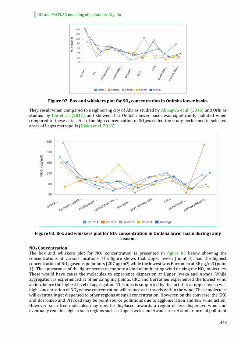
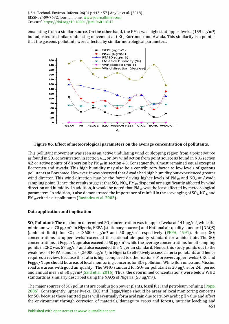
Effect of meteorological parameters The effect of meteorological parameters on the studied variables were plotted in the figure 06 below. The diagram showed that the wind speed was well below 10ms-1 and had little or no effect on the SO2, NO2, and PM10 determinants. The average plot of NO2 and SO2 were almost superimposable at each sampling point. The highest NO2 was at CKC at 155ug/m3 while SO2 at CKC was 57ug/m3. Hence, this may be



emanating from a similar source. On the other hand, the PM10 was highest at upper Iweka (159 ug/m3) but adjusted to similar undulating movement at CKC, Borromeo and Awada. This similarity is a pointer that the gaseous pollutants were affected by similar metrological parameters.

IWEKA PH FEGGE UZO MISSION REST C.K.C BORO AWADA

0

20

40

60

80

100

120

140

160

180

200

220

240

260

A

SO2 (ug/m3)

NO2 (ug/m3)

PM10 (ug/m3)

Relative humidity (%)

Windspeed (ms-1)

Wind direction (degree)

Figure 06. Effect of meteorological parameters on the average concentration of pollutants.

This pollutant movement was seen as an active undulating wind or slopping region from a point source as found in SO2 concentration in section 4.1, or low wind action from point source as found in NO2 section 4.2 or active points of dispersion by PM10 in section 4.3. Consequently, almost remained equal except at Borromeo and Awada. This high humidity may also be a contributory factor to low levels of gaseous pollutants at Borromeo. However, it was observed that Awada had high humidity but experienced greater wind director. This wind direction may be the force driving higher levels of PM10 and NO2 at Awada sampling point. Hence, the results suggest that SO2, NO2, PM10 dispersal are significantly affected by wind direction and humidity. In addition, it would be noted that PM10 was the least affected by meteorological parameters. In addition, it also demonstrated the importance of rainfall in the scavenging of SO2, NO2, and PM10 criteria air pollutants (Ravindra et al. 2003).

Data application and implication

SO2 Pollutant: The maximum determined SO2concentration was in upper Iweka at 141 µg/m3, while the minimum was 70 µg/m3. In Nigeria, FEPA (stationary sources) and National air quality standard (NAQS) (ambient limit) for SO2 is 26000 µg/m3 and 50 µg/m3 respectively (FEPA, 1991). Hence, SO2 concentrations at upper Iweka exceeded the national air quality standard for ambient air. The SO2 concentrations at Fegge/Nupe also exceeded 50 µg/m3, while the average concentrations for all sampling points in CKC was 57 µg/m3 and also exceeded the Nigerian standard. Hence, this study points out to the weakness of FEPA standards (26000 µg/m3) in Nigeria to effectively access criteria pollutants and hence requires a review. Because this ratio is high compared to other nations. Moreover, upper Iweka, CKC and Fegge/Nupe should be areas of local monitoring concerns for SO2 pollution. While Borromeo and Mission road are areas with good air quality. The WHO standard for SO2 air pollutant is 20 µg/m3for 24h period and annual mean of 50 µg/m3 (Said et al. 2016). Thus, the determined concentrations were below WHO standards as similarly described using the NAQS of Nigeria (50 µg/m3).

The major sources of SO2 pollutant are combustion power plants, fossil fuel and petroleum refining (Popp, 2006). Consequently, upper Iweka, CKC and Fegge/Nupe should be areas of local monitoring concerns for SO2 because these emitted gases will eventually form acid rain due to its low acidic pH value and affect the environment through corrosion of materials, damage to crops and forests, nutrient leaching and



452

contaminating drinking water. Additionally, since SO2 residence time is 2 to 4 days and its main dispersion is by oxidation (Griffin, 2006). The enforcement of standards and map transport within areas of upper Iweka, CKC and Fegge/Nupe and gas transport are required for SO2 pollutant control in Onitsha Lower basin.

NO2 Pollutant: The maximum values of NO2 determined was 109 µg/m3 at Upper Iweka, while the minimum value was measured at Borromeo to be 19 µg/m3. The values when compared with FEPA (stationary sources) and National air quality standard (NAQS) (ambient limit) for NO2 is 75000 µg/m3 and 1000 µg/m3 respectively (FEPA, 1991). Thus, the levels of NO2 at all sampling points were below Nigeria standard and accordingly, all areas have good air quality with respect to NO2. Additionally, WHO 1h mean is 200 ug/m3, while annual mean period is 40 µg/m3 (Said et al. 2016) Subsequently, the average concentration of NO2 for all sampling points exceeded 40 µg/m3 except at Borromeo with 28 µg/m3. Since the average level of NO2 exceeded WHO mean annual level, there is therefore the possibility of reacting with water to form acid rain in all sampled regions. These would lead to material corrosion and damage to crops. Moreover, the NO2 residence time is 2-5 days, while principal sinks occur through oxidation, deposition, photolysis and dissolution in oceans and surface waters. Thus, if the major sources were fossil fuel combustion driving the NO2fluxes, there is the need for monitoring trans-boundary fluxes from stationary and mobile sources. Also, the use of selective non-catalyst reduction technology in such combustion processes will further reduce the release of nitrogen oxides (Popp, 2006; Griffin, 2006).

PM10 Pollutants: The maximum determined PM10 concentration was 111 µg/m3determined at both Upper Iweka and pH road. The minimum determined concentration was at Borromeo at 58 µg/m3. Their comparison to Nigeria, FEPA (stationary sources) and National air quality standard (NAQS) (ambient limit) for PM10 is 25000 µg/m3and 150 µg/m3 respectively. Accordingly, the concentration levels were lower than FEPA and NAQs standards. Also, this illustrated the inability of FEPA at such high standard (25000 ug/m3) to effectively evaluate criteria pollutants that are noxious even at low concentrations. The WHO standard for PM10 is 20 µg/m3for 24h period and annual mean of 50 µg/m3 (FEPA, 1991). Thus, the sampled area exceeded the WHO standard with respect to PM10. But since PM10 has particle size < 10um, they are mostly released by combustion of fossil fuels, motor vehicles, agricultural burning and industrial activities.

Such activities can prevent suns radiation from reaching the earth when they act as cloud nuclei. they effect is reduced visibility, depletion of soil nutrients, acidification of surface water and destruction of sensitive ecological forests and farm crops. Consequently, there should be controls for industrial facilities, motor vehicles and use of cleaner burning gasoline and diesel fuels (Akinfolarin et al. 2017; Opara et al. 2016; Popp, 2006; Griffin, 2006).

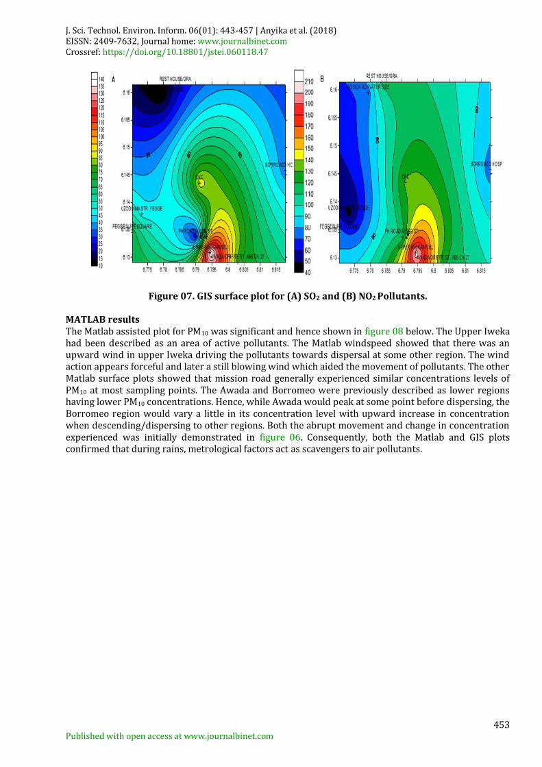
GIS plot The GIS plot was shown in figure 07 below. These provided a better and elaborate description of the concentrations of the pollutant relative to their respective positions. The highest concentration of SO2 (A) can be clearly seen to be Upper Iweka and Awada and was similarly observed in NO2 plot (B). Borromeo and Mission road/waterside were the lowest points of concentration for NO2 and SO2 respectively. The contours showed that that pollutants spreads from Awada and Upper Iweka to other sampling regions. Three or more central forces were active in SO2, while about two could be seen in NO2. This demonstrated that SO2 is more quickly dispersed than NO2. A similar dispersion movement was observed in PM10 with Upper Iweka showing highest concentration and spreading towards CKC. One central force was observed in PM10 and hence, dispersed at a speed slower than NO2. Summarily the SO2 was the most active gaseous pollutant and more easily dispersed by metrological forces (wind speed, wind direction, humidity) than NO2 and PM10. These showed a correlation with section 4.5 that the studied pollutants were affected by metrological factors in the order of SO2> NO2> PM10.



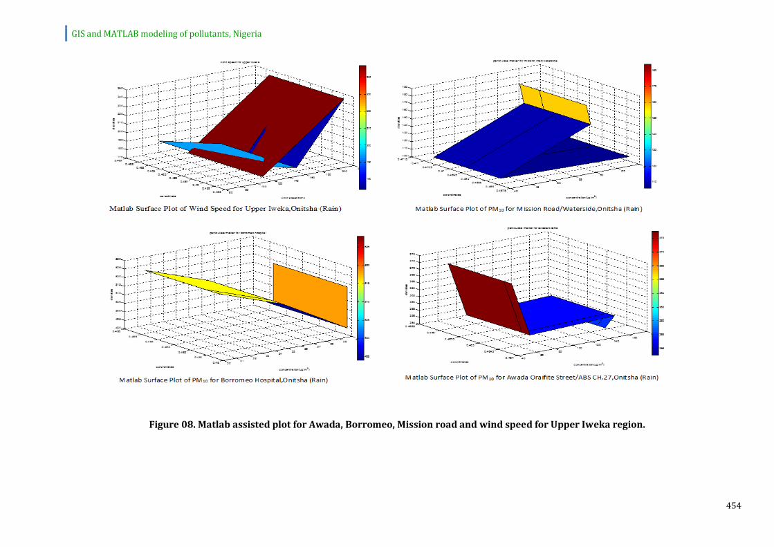
Figure 07. GIS surface plot for (A) SO2 and (B) NO2 Pollutants. MATLAB results The Matlab assisted plot for PM10 was significant and hence shown in figure 08 below. The Upper Iweka had been described as an area of active pollutants. The Matlab windspeed showed that there was an upward wind in upper Iweka driving the pollutants towards dispersal at some other region. The wind action appears forceful and later a still blowing wind which aided the movement of pollutants. The other Matlab surface plots showed that mission road generally experienced similar concentrations levels of PM10 at most sampling points. The Awada and Borromeo were previously described as lower regions having lower PM10 concentrations. Hence, while Awada would peak at some point before dispersing, the Borromeo region would vary a little in its concentration level with upward increase in concentration when descending/dispersing to other regions. Both the abrupt movement and change in concentration experienced was initially demonstrated in figure 06. Consequently, both the Matlab and GIS plots confirmed that during rains, metrological factors act as scavengers to air pollutants.



454

Figure 08. Matlab assisted plot for Awada, Borromeo, Mission road and wind speed for Upper Iweka region.



IV. Conclusion

The study of air pollutants utilizing spatial processing and time series analysis has seen accurate results for regulatory purposes in densely populated cities. GPS and MATLAB modeling utilized in this study for SO2, NO2 and PM10 pollutants during rains in Lower Onitsha basin. The named pollutants were studied at different measuring times in nine locations for 3 months of rains in three consecutive years. A Matlab model was generated by polynomial equations while GIS coordinates were mapped using ARCGIS 9.3. All the 3 pollutants showed highest concentrations at Upper Iweka and dispersed towards Awada, Borromeo or Rest house. AQI showed that PM10 and NO2 may affect sensitive groups at Upper Iweka, Awada and PH road. SO2 levels were below WHO standard but NO2 and PM10 average concentrations exceeded the WHO standard. Additionally, the study revealed the inability of FEPA at such high standard (26000 for SO2, 75000 for NO2 and 25000 for PM10 µg/m3) to effectively evaluate criteria pollutants that are noxious even at low concentrations The Metamodeling and GIS mapping identified wind speed, wind direction and humidity as effective scavengers of SO2, NO2 and PM10. Hence, the study demonstrated that Upper Iweka is a major point source pollution and scavenged by wind speed, wind direction and humidity under prevailing rains in onitsha lower basin.

Acknowledgement

The author Anyika L. C wishes to acknowledge the supervisors of this work including Prof. G. N. Onuoha, Prof. E. N. Ejike and Dr. A. I. Opara and all other contributory authors including Alisa C.O and Nkwoada A.U who managed the research protocol, statistical analysis and wrote the manuscript.

Conflict of Interest

The authors declare that no conflict of interest exists.

V. References

[1]. Akinfolarin, O. Boisa, N. and Obunwo, C. (2017). Assessment of particulate matter-based air quality index in Port Harcourt, Nigeria. Journal of Environmental Analytical Chemistry, 4(224), 1-4. https://doi.org/10.4172/2380-2391.1000224

[2]. Akuagwu, N. Ejike, E. and Kalu, A. (2016). Estimation of air quality in Aba urban, Nigeria using the multiple linear regression technique. Journal of Geography, Environment and Earth Science International, 4(2), 1-6. https://doi.org/10.9734/JGEESI/2016/21931

[3]. Ambare, M. and Muhammed, L. (2013). The role of GIS and remote sensing in mapping the distribution of greenhouse gases. European Scientific Journal, 9(36), 404-410.

[4]. Ankita, P. Rohit, G. and Pran, N. (2017). Assessment of spatio-temporal variations in air quality of Jaipur city,Rajasthan, India. The Egyptian Journal of Remote Sensing and Space Sciences, 1-9.

[5]. Balogun, V. and Orimoogunje, I. (2015). An assessment of seasonal variation of air pollution in Benin city, Southern Nigeria. Atmospheric and Climate Sciences, 5, 209-218. https://doi.org/10.4236/acs.2015.53015

[6]. Beckx, C. Panis, L. Janssens, D. and Wets, G. (2010). Applying activity-travel data for the assessment of vehicle exhaust emissions: Application of a GPS-enhanced data collection tool. Transportation Research Part D, 5, 117-122. https://doi.org/10.1016/j.trd.2009.10.004

[7]. Buckland, K. Young, S. Keim, E. Johnson, R. Johnson, P. and Tratt, D. (2017). Tracking and quantification of gaseous chemical plumes from anthropogenic emission sources within the Los Angeles Basin. Remote Sensing of Environment, 201, 275-296. https://doi.org/10.1016/j.rse.2017.09.012

[8]. Challoner, A. Pilla, F. and Gill, L. (2015). Prediction of indoor air exposure from outdoor air quality using an artificial neural network model for inner city commercial buildings. International Journal of Environmental Research and Public Health, 12, 15233-15253. https://doi.org/10.3390/ijerph121214975


https://doi.org/10.4172/2380-2391.1000224

https://doi.org/10.9734/JGEESI/2016/21931

https://doi.org/10.4236/acs.2015.53015

https://doi.org/10.1016/j.trd.2009.10.004

https://doi.org/10.1016/j.rse.2017.09.012

https://doi.org/10.3390/ijerph121214975


456

[9]. Environmental Protection Agency, USA (2016). Air Now. (N. C. Durham, Producer, & Durham, North Carolina) Retrieved May 28, 2018, from Air Calculator: https://www.airnow.gov/index.cfm?action=aqibasics.aqi.

[10]. FEPA, Federal Environmental Protection Agency (1991). National interim guidelines and standards for industrial effluents, gaseous emissions and Hazardous wastes. Environmental Pollution Control Handbook. Lagos.

[11]. GNI, Geoscience News and Information (2017). Geology.com. (Geology.com, Producer) Retrieved April 12, 2018, from Nigeria Map and Satellite Image: https://geology.com/world/nigeria-satellite-image.shtml

[12]. Google (2018). Google earth. (Google) Retrieved January 15, 2018, from Google earth: https://www.google.com/earth/

[13]. Griffin, R. (2006). Principles of air quality management (2nd ed.). New York, New York, USA: Taylor and Francis.

[14]. Ibe, F. Opara, A. Njoku, P. and Alinnor, J. (2017). Ambient air quality assessment of Orlu, southeastern, Nigeria. Journal of Applied Sciences, 441-457.

[15]. Jiayu, L. Haoran, L. Yehan, M. Yang, W. Ahmed, A. Chenyang, L. and Pratim, B. (2018). Spatiotemporal distribution of indoor particulate matter concentration with a low-cost sensor network. Building and Environment, 127, 138-147. https://doi.org/10.1016/j.buildenv.2017.11.001

[16]. Kanchan, A. and Goyal, P. (2015). A review on air quality indexing system. Asian Journal of Atmospheric Environment, 9(2), 101-113. https://doi.org/10.5572/ajae.2015.9.2.101

[17]. Njoku, K. Rumide, T. Akinola, M. Adesuyi, A. and Jolaoso, A. (2016). Ambient air quality monitoring in metropolitan city of Lagos, Nigeria. Journal of Applied Science and Environmrntal Management, 20(1), 178-185.

[18]. Nkwoada, A. Oguzie, E. Alisa, C. Agwaramgbo, L. and Enenebeaku, C. (2016). Emissions of gasoline combustion by products in automotive exhausts. International Journal of Scientific and Research Publications, 6(4), 464-482.

[19]. Omotosho, T. Emetere, M. and Arase, O. (2015). Mathematical projections of air pollutants effects over Niger Delta Region using remotely sensed satellite data. International Journal of Applied Environmental Sciences, 10(2), 6651-6664.

[20]. Opara, A. Ibe, F. Njoku, P. Alinnor, J. and Enenebeaku, C. (2016). Geospatial and Geostatistical Analyses of Particulate Matter (PM10). International Letters of Natural Sciences, 57, 89-107. https://doi.org/10.18052/www.scipress.com/ILNS.57.89

[21]. Palomera, J. Alvarez, B. Echeverria, S. Hernandez, E. Alvarez, P. and Villegas, R. (2016). Photochemical assessment monitoring stations program adapted for ozone precursors monitoring network in Mexico City. Atmosfera, 29(2), 169-188. https://doi.org/10.20937/ATM.2016.29.02.06

[22]. Park, D. Kwon, S. and Cho, Y. (2013). Development and calibration of a particulate matter measurement device with wireless sensor network function. International Journal of Environmental Monitoring and Analysis, 1(1), 15-30. https://doi.org/10.11648/j.ijema.20130101.12

[23]. Partheeban, P. Hemamalini, R. and Raju, P. (2012). Vehicular emission monitoring using internet GIS, GPS and sensors. International Conference on Environment, Energy and Biotechnology, 33, 82-85.

[24]. Pilla, F. and Broderick, B. (2015). A GIS model for personal exposure to PM10 for Dublin commuters. Sustainable Cities and Society, 15, 1-10. https://doi.org/10.1016/j.scs.2014.10.005

[25]. Popp, D. (2006). International innovation and diffusion of air pollution control technologies: the effects of NOX and SO2 regulation in the US, Japan, and Germany. Journal of Environmental Economics and Management, 51(1), 46-71. https://doi.org/10.1016/j.jeem.2005.04.006

[26]. Puliafito, E. Guevara, M. and Puliafito, C. (2003). Characterization of urban air quality using GIS as a management system. Environmental Pollution, 112, 105-117. https://doi.org/10.1016/S0269-7491(02)00278-6

[27]. Raju, P. Partheeban, P. and Hemamalini, R. (2012). Urban mobile air quality monitoring using GIS, GPS, sensors and internet. International Journal of Environmental Science and Development, 3(4), 324-327. https://doi.org/10.7763/IJESD.2012.V3.240

https://www.airnow.gov/index.cfm?action=aqibasics.aqi.

https://geology.com/world/nigeria-satellite-image.shtml

https://geology.com/world/nigeria-satellite-image.shtml

https://www.google.com/earth/

https://doi.org/10.1016/j.buildenv.2017.11.001

https://doi.org/10.5572/ajae.2015.9.2.101

https://doi.org/10.18052/www.scipress.com/ILNS.57.89

https://doi.org/10.20937/ATM.2016.29.02.06

https://doi.org/10.11648/j.ijema.20130101.12

https://doi.org/10.1016/j.scs.2014.10.005

https://doi.org/10.1016/j.jeem.2005.04.006

https://doi.org/10.1016/S0269-7491(02)00278-6

https://doi.org/10.1016/S0269-7491(02)00278-6

https://doi.org/10.7763/IJESD.2012.V3.240



[28]. Ravindra, K. Ameena, S. Kamyotra, J. and Kaushik, C. (2003). Variation in spatial pattern of criteria air pollutants before and during rain of monsoon. Environmental Monitoring and Assessment, 87, 145-153. https://doi.org/10.1023/A:1024650215970

[29]. Rohde, R. and Muller, R. (2015). Air pollution in China: Mapping of concentrations and sources. PLoS ONE, 10(8), 1-14. https://doi.org/10.1371/journal.pone.0135749

[30]. Said, M. Safwat, G. Turki, M. and Mamoun, A. (2016). Spatiotemporal analysis of fine particulate matter (PM2.5) in Saudi Arabia using remote sensing data. The Egyptian Journal of Remote Sensing and Space Sciences, 12(2), 195-205.

[31]. Wei, C. Lei, Y.anf Haimeng, Z. (2015). Seasonal variations of atmospheric pollution and air quality in Beijing. Atmosphere, 6, 1753-1770. https://doi.org/10.3390/atmos6111753

[32]. Ying, X. Wenjun, W. Baochang, L. Zhiwei, Z. Lei, H. and Yaxin, W. (2017). Analysis of SO2 Pollution in Baoding based on MATLAB grey model. Chemical Engineering Transactions, 59, 901-906.

[33]. Yorkor, B. Leton, T. and Ugbebor, J. (2017). Prediction and modeling of seasonal concentrations of air pollutants in semi-urban region employing artiicial neural network ensembles. International Journal of Environment and Pollution Research, 5(3), 1-18.

[34]. Youping, L. Ya, T. Zhongyu, F. Hong, Z. and Zhengzheng, Y. (2018). Assessment and comparison of three different air quality indices in China. Environmental Engineering and Research, 23(1), 21-27.

[35]. Zhao, L. Meihui, X. Kun, T. and Peichao, G. (2017). GIS-based analysis of population exposure to PM2.5 air pollution-A case study of Beijing. Journal of Environmental Sciences, 1-7.

HOW TO CITE THIS ARTICLE? Crossref: https://doi.org/10.18801/jstei.060118.47

MLA Anyika et al. “GIS and MATLAB modeling of criteria pollutants: a study of lower Onitsha basin during rains”. Journal of Science, Technology and Environment Informatics 06(01) (2018): 443-457. APA Anyika, L. C. Alisa, C. O. Nkwoada, A. U. Opara, A. I. Ejike, E. N. and Onuoha, G. N. (2018). GIS and MATLAB modeling of criteria pollutants: a study of lower Onitsha basin during rains. Journal of Science, Technology and Environment Informatics, 06(01), 443-457. Chicago Anyika, L. C. Alisa, C. O. Nkwoada, A. U. Opara, A. I. Ejike, E. N. and Onuoha, G. N. “GIS and MATLAB modeling of criteria pollutants: a study of lower Onitsha basin during rains.” Journal of Science, Technology and Environment Informatics 06(01) (2018): 443-457. Harvard Anyika, L. C. Alisa, C. O. Nkwoada, A. U. Opara, A. I. Ejike, E. N. and Onuoha, G. N. 2018. GIS and MATLAB modeling of criteria pollutants: a study of lower Onitsha basin during rains. Journal of Science, Technology and Environment Informatics, 06(01), pp. 443-457. Vancouver Anyika, LC, Alisa, CO, Nkwoada, AU, Opara, AI, Ejike, EN and Onuoha, GN. GIS and MATLAB modeling of criteria pollutants: a study of lower Onitsha basin during rains. Journal of Science, Technology and Environment Informatics. 2018 October 06(01): 443-457.


https://doi.org/10.1023/A:1024650215970

https://doi.org/10.1371/journal.pone.0135749

https://doi.org/10.3390/atmos6111753


Documents

GIS and MATLAB modeling of criteria pollutants: a …...GIS and MATLAB modeling of pollutants, Nigeria 444 artificial neural network assemblage (ANN), for outdoor air quality. The