Gibbs Measures and Phase Transitions on Sparse Random Graphsmontanar/RESEARCH/FILEPAP/full-version.pdf · Dembo et al./Gibbs Measures on Sparse Random Graphs 3 associated with the

Gibbs Measures and Phase Transitions on

Sparse Random Graphs

Amir Dembo ∗ , Andrea Montanari ∗

Stanford University.e-mail: [email protected]; [email protected]

Abstract: Many problems of interest in computer science and informa-tion theory can be phrased in terms of a probability distribution overdiscrete variables associated to the vertices of a large (but finite) sparsegraph. In recent years, considerable progress has been achieved by view-ing these distributions as Gibbs measures and applying to their studyheuristic tools from statistical physics. We review this approach andprovide some results towards a rigorous treatment of these problems.

AMS 2000 subject classifications: Primary 60B10, 60G60, 82B20.Keywords and phrases: Random graphs, Ising model, Gibbs mea-sures, Phase transitions, Spin models, Local weak convergence..

Contents

1 Introduction . . . . . . . . . . . . . . . . . . . . . . . . . . . . . . . 21.1 The Curie-Weiss model and some general definitions . . . . . 41.2 Graphical models: examples . . . . . . . . . . . . . . . . . . . 131.3 Detour: The Ising model on the integer lattice . . . . . . . . . 18

2 Ising models on locally tree-like graphs . . . . . . . . . . . . . . . . 212.1 Locally tree-like graphs and conditionally independent trees . 222.2 Ising models on conditionally independent trees . . . . . . . . 292.3 Algorithmic implications: belief propagation . . . . . . . . . . 322.4 Free entropy density, from trees to graphs . . . . . . . . . . . 332.5 Coexistence at low temperature . . . . . . . . . . . . . . . . . 36

3 The Bethe-Peierls approximation . . . . . . . . . . . . . . . . . . . 403.1 Messages, belief propagation and Bethe equations . . . . . . . 413.2 The Bethe free entropy . . . . . . . . . . . . . . . . . . . . . . 443.3 Examples: Bethe equations and free entropy . . . . . . . . . . 473.4 Extremality, Bethe states and Bethe-Peierls approximation . 52

4 Colorings of random graphs . . . . . . . . . . . . . . . . . . . . . . 574.1 The phase diagram: a broad picture . . . . . . . . . . . . . . 58

∗Research partially funded by NSF grant #DMS-0806211.

1

imsart-generic ver. 2009/08/13 file: full-version.tex date: October 28, 2009

Dembo et al./Gibbs Measures on Sparse Random Graphs 2

4.2 The COL-UNCOL transition . . . . . . . . . . . . . . . . . . 604.3 Coexistence and clustering: the physicist’s approach . . . . . 62

5 Reconstruction and extremality . . . . . . . . . . . . . . . . . . . . 715.1 Applications and related work . . . . . . . . . . . . . . . . . . 735.2 Reconstruction on graphs: sphericity and tree-solvability . . . 765.3 Proof of main results . . . . . . . . . . . . . . . . . . . . . . . 79

6 XORSAT and finite-size scaling . . . . . . . . . . . . . . . . . . . . 856.1 XORSAT on random regular graphs . . . . . . . . . . . . . . 876.2 Hyper-loops, hypergraphs, cores and a peeling algorithm . . . 916.3 The approximation by a smooth Markov kernel . . . . . . . . 936.4 The ODE method and the critical value . . . . . . . . . . . . 986.5 Diffusion approximation and scaling window . . . . . . . . . . 1016.6 Finite size scaling correction to the critical value . . . . . . . 102

References . . . . . . . . . . . . . . . . . . . . . . . . . . . . . . . . . . 106

1. Introduction

Statistical mechanics is a rich source of fascinating phenomena that can be,at least in principle, fully understood in terms of probability theory. Overthe last two decades, probabilists have tackled this challenge with much suc-cess. Notable examples include percolation theory [49], interacting particlesystems [61], and most recently, conformal invariance. Our focus here is onanother area of statistical mechanics, the theory of Gibbs measures, whichprovides a very effective and flexible way to define collections of ‘locallydependent’ random variables.

The general abstract theory of Gibbs measures is fully rigorous from amathematical point of view [42]. However, when it comes to understandingthe properties of specific Gibbs measures, i.e. of specific models, a large gappersists between physicists heuristic methods and the scope of mathemati-cally rigorous techniques.

This paper is devoted to somewhat non-standard, family of models, namelyGibbs measures on sparse random graphs. Classically, statistical mechanicshas been motivated by the desire to understand the physical behavior of ma-terials, for instance the phase changes of water under temperature change,or the permeation or oil in a porous material. This naturally led to three-dimensional models for such phenomena. The discovery of ‘universality’ (i.e.the observation that many qualitative features do not depend on the micro-scopic details of the system), led in turn to the study of models on three-dimensional lattices, whereby the elementary degrees of freedom (spins) are



associated with the vertices of of the lattice. Thereafter, d-dimensional lat-tices (typically Zd), became the object of interest upon realizing that signif-icant insight can be gained through such a generalization.

The study of statistical mechanics models ‘beyond Zd’ is not directlymotivated by physics considerations. Nevertheless, physicists have been in-terested in models on other graph structures for quite a long time (an earlyexample is [36]). Appropriate graph structures can simplify considerably thetreatment of a specific model, and sometimes allow for sharp predictions.Hopefully some qualitative features of this prediction survive on Zd.

Recently this area has witnessed significant progress and renewed interestas a consequence of motivations coming from computer science, probabilis-tic combinatorics and statistical inference. In these disciplines, one is ofteninterested in understanding the properties of (optimal) solutions of a largeset of combinatorial constraints. As a typical example, consider a linear sys-tem over GF[2], Ax = b mod 2, with A an n × n binary matrix and b abinary vector of length n. Assume that A and b are drawn from randommatrix/vector ensemble. Typical questions are: What is the probability thatsuch a linear system admits a solution? Assuming a typical realization doesnot admit a solution, what is the maximum number of equations that can,typically, be satisfied?

While probabilistic combinatorics developed a number of ingenious tech-niques to deal with these questions, significant progress has been achieved re-cently by employing novel insights from statistical physics (see [65]). Specif-ically, one first defines a Gibbs measure associated to each instance of theproblem at hand, then analyzes its properties using statistical physics tech-niques, such as the cavity method. While non-rigorous, this approach ap-pears to be very systematic and to provide many sharp predictions.

It is clear at the outset that, for ‘natural’ distributions of the binarymatrix A, the above problem does not have any d-dimensional structure.Similarly, in many interesting examples, one can associate to the Gibbsmeasure a graph that is sparse and random, but of no finite-dimensionalstructure. Non-rigorous statistical mechanics techniques appear to providedetailed predictions about general Gibbs measures of this type. It would behighly desirable –and in principle possible– to develop a fully mathemat-ical theory of such Gibbs measures. The present paper provides a unifiedpresentation of a few results in this direction.

In the rest of this section, we proceed with a more detailed overview of thetopic, proposing certain fundamental questions the answer to which playsan important role within the non-rigorous statistical mechanics analysis. Weillustrate these questions on the relatively well-understood Curie-Weiss (toy)



model and explore a few additional motivating examples.Section 2 focuses on a specific example, namely the ferromagnetic Ising

model on sequences of locally tree-like graphs. Thanks to its monotonicityproperties, detailed information can be gained on this model.

A recurring prediction of statistical mechanics studies is that Bethe-Peierls approximation is asymptotically tight in the large graph limit, forsequences of locally tree-like graphs. Section 3 provides a mathematical for-malization of Bethe-Peierls approximation. We also prove there that, underan appropriate correlation decay condition, Bethe-Peierls approximation isindeed essentially correct on graphs with large girth.

In Section 4 we consider a more challenging, and as of now, poorly under-stood, example: proper colorings of a sparse random graph. A fascinating‘clustering’ phase transition is predicted to occur as the average degree of thegraph crosses a certain threshold. Whereas the detailed description and ver-ification of this phase transition remains an open problem, its relation withthe appropriate notion of correlation decay (‘extremality’), is the subject ofSection 5.

Finally, it is common wisdom in statistical mechanics that phase transi-tions should be accompanied by a specific ‘finite-size scaling’ behavior. Moreprecisely, a phase transition corresponds to a sharp change in some propertyof the model when a control parameter crosses a threshold. In a finite sys-tem, the dependence on any control parameter is smooth, and the changeand takes place in a window whose width decreases with the system size.Finite-size scaling broadly refers to a description of the system behaviorwithin this window. Section 6 presents a model in which finite-size scalingcan be determined in detail.

1.1. The Curie-Weiss model and some general definitions

The Curie-Weiss model is deceivingly simple, but is a good framework tostart illustrating some important ideas. For a detailed study of this modelwe refer to [37].

1.1.1. A story about opinion formation

At time zero, each of n individuals takes one of two opinions Xi(0) ∈+1,−1 independently and uniformly at random for i ∈ [n] = 1, . . . , n.At each subsequent time t, one individual i, chosen uniformly at random,



computes the opinion imbalance

M ≡n∑

j=1

Xj , (1.1)

and M (i) ≡M −Xi. Then, he/she changes his/her opinion with probability

pflip(X) =

exp(−2β|M (i)|/n) if M (i)Xi > 0 ,1 otherwise.

(1.2)

Despite its simplicity, this model raises several interesting questions.

(a). How long does is take for the process X(t) to become approximatelystationary?

(b). How often do individuals change opinion in the stationary state?(c). Is the typical opinion pattern strongly polarized (herding)?(d). If this is the case, how often does the popular opinion change?

We do not address question (a) here, but we will address some version ofquestions (b)–(d). More precisely, this dynamics (first studied in statisticalphysics under the name of Glauber or Metropolis dynamics) is an aperiodicirreducible Markov chain whose unique stationary measure is

µn,β(x) =1

Zn(β)exp

βn

∑

(i,j)

xixj. (1.3)

To verify this, simply check that the dynamics given by (1.2) is reversiblewith respect to the measure µn,β of (1.3). Namely, that µn,β(x)P(x→ x′) =µn,β(x

′)P(x′ → x) for any two configurations x, x′ (where P(x→ x′) denotesthe one-step transition probability from x to x′).

We are mostly interested in the large-n (population size), behavior ofµn,β(·) and its dependence on β (the interaction strength). In this context,we have the following ‘static’ versions of the preceding questions:

(b’). What is the distribution of pflip(x) when x has distribution µn,β( · )?(c’). What is the distribution of the opinion imbalance M? Is it concen-

trated near 0 (evenly spread opinions), or far from 0 (herding)?(d’). In the herding case: how unlikely are balanced (M ≈ 0) configurations?

1.1.2. Graphical models

A graph G = (V,E) consists of a set V of vertices and a set E of edges(where an edge is an unordered pair of vertices). We always assume G to



be finite with |V | = n and often make the identification V = [n]. With Xa finite set, called the variable domain, we associate to each vertex i ∈ Va variable xi ∈ X , denoting by x ∈ X V the complete assignment of thesevariables and by xU = xi : i ∈ U its restriction to U ⊆ V .

Definition 1.1. A bounded specification ψ ≡ ψij : (i, j) ∈ E for a graphG and variable domain X is a family of functionals ψij : X ×X → [0, ψmax]indexed by the edges of G with ψmax a given finite, positive constant (wherefor consistency ψij(x, x

′) = ψji(x′, x) for all x, x′ ∈ X and (i, j) ∈ E). The

specification may include in addition functions ψi : X → [0, ψmax] indexedby vertices of G.

A bounded specification ψ for G is permissive if there exists a positiveconstant κ and a ‘permitted state’ xp

i ∈ X for each i ∈ V , such thatmini,x′ ψi(x

′) ≥ κψmax and

min(i,j)∈E,x′∈X

ψij(xpi , x

′) = min(i,j)∈E,x′∈X

ψij(x′, xp

j ) ≥ κψmax ≡ ψmin .

The graphical model associated with a graph-specification pair (G,ψ) isthe canonical probability measure

µG,ψ(x) =1

Z(G,ψ)

∏

(i,j)∈Eψij(xi, xj)

∏

i∈Vψi(xi) (1.4)

and the corresponding canonical stochastic process is the collection X =Xi : i ∈ V of X -valued random variables having joint distribution µG,ψ(·).

One such example is the distribution (1.3), where X = +1,−1, G isthe complete graph over n vertices and ψij(xi, xj) = exp(βxixj/n). Hereψi(x) ≡ 1. It is sometimes convenient to introduce a ‘magnetic field’ (see forinstance Eq. (1.9) below). This corresponds to taking ψi(xi) = exp(Bxi).

Rather than studying graphical models at this level of generality, we focuson a few concepts/tools that have been the subject of recent research efforts.

Coexistence. Roughly speaking, we say that a model (G,ψ) exhibitscoexistence if the corresponding measure µG,ψ(·) decomposes into a convexcombination of well-separated lumps. To formalize this notion, we considersequences of measures µn on graphs Gn = ([n], En), and say that coex-istence occurs if, for each n, there exists a partition Ω1,n, . . . ,Ωr,n of theconfiguration space X n with r = r(n) ≥ 2, such that

(a). The measure of elements of the partition is uniformly bounded away



from one:

max1≤s≤r

µn(Ωs,n) ≤ 1 − δ . (1.5)

(b). The elements of the partition are separated by ‘bottlenecks’. That is,for some ǫ > 0,

max1≤s≤r

µn(∂ǫΩs,n)

µn(Ωs,n)→ 0 , (1.6)

as n→ ∞, where ∂ǫΩ denotes the ǫ-boundary of Ω ⊆ X n,

∂ǫΩ ≡ x ∈ X n : 1 ≤ d(x,Ω) ≤ nǫ , (1.7)

with respect to the Hamming 1 distance. The normalization by µn(Ωs,n)removes ‘false bottlenecks’ and is in particular needed since r(n) oftengrows (exponentially) with n.Depending on the circumstances, one may further specify a requiredrate of decay in (1.6).

We often consider families of models indexed by one (or more) continuousparameters, such as the inverse temperature β in the Curie-Weiss model. Aphase transition will generically be a sharp threshold in some property ofthe measure µ( · ) as one of these parameters changes. In particular, a phasetransition can separate values of the parameter for which coexistence occursfrom those values for which it does not.

Mean field models. Intuitively, these are models that lack any (finite-dimensional) geometrical structure. For instance, models of the form (1.4)with ψij independent of (i, j) and G the complete graph or a regular randomgraph are mean field models, whereas models in which G is a finite subsetof a finite dimensional lattice are not. To be a bit more precise, the Curie-Weiss model belongs to a particular class of mean field models in which themeasure µ(x) is exchangeable (that is, invariant under coordinate permuta-tions). A wider class of mean field models may be obtained by consideringrandom distributions2 µ(·) (for example, when either G or ψ are chosen atrandom in (1.4)). In this context, given a realization of µ, consider k i.i.d.

1The Hamming distance d(x, x′) between configurations x and x′ is the number ofpositions in which the two configurations differ. Given Ω ⊆ Xn, d(x, Ω) ≡ mind(x, x′) :x′ ∈ Ω.

2A random distribution over Xn is just a random variable taking values on the (|X |n −1)-dimensional probability simplex.



configurations X(1), . . . ,X(k), each having distribution µ. These ‘replicas’have the unconditional, joint distribution

µ(k)(x(1), . . . , x(k)) = Eµ(x(1)) · · · µ(x(k))

. (1.8)

The random distribution µ is a candidate to be a mean field model whenfor each fixed k the measure µ(k), viewed as a distribution over (X k)n, isexchangeable (with respect to permutations of the coordinate indices in[n]). Unfortunately, while this property suffices in many ‘natural’ specialcases, there are models that intuitively are not mean-field and yet haveit. For instance, given a non-random measure ν and a uniformly randompermutation π, the random distribution µ(x1, . . . , xn) ≡ ν(xπ(1), . . . , xπ(n))meets the preceding requirement yet should not be considered a mean fieldmodel. While a satisfactory mathematical definition of the notion of meanfield models is lacking, by focusing on selective examples we examine in thesequel the rich array of interesting phenomena that such models exhibit.

Mean field equations. Distinct variables may be correlated in the model(1.4) in very subtle ways. Nevertheless, mean field models are often tractablebecause an effective ‘reduction’ to local marginals3 takes place asymptoti-cally for large sizes (i.e. as n→ ∞).

Thanks to this reduction it is often possible to write a closed system ofequations for the local marginals that hold in the large size limit and de-termine the local marginals, up to possibly having finitely many solutions.Finding the ‘correct’ mathematical definition of this notion is an open prob-lem, so we shall instead provide specific examples of such equations in a fewspecial cases of interest (starting with the Curie-Weiss model).

1.1.3. Coexistence in the Curie-Weiss model

The model (1.3) appeared for the first time in the physics literature as amodel for ferromagnets4. In this context, the variables xi are called spins andtheir value represents the direction in which a localized magnetic moment(think of a tiny compass needle) is pointing. In certain materials the differentmagnetic moments favor pointing in the same direction, and physicists wantto know whether such interaction may lead to a macroscopic magnetization(imbalance), or not.

3In particular, single variable marginals, or joint distributions of two variables con-nected by an edge.

4A ferromagnet is a material that acquires a macroscopic spontaneous magnetizationat low temperature.



In studying this and related problems it often helps to slightly general-ize the model by introducing a linear term in the exponent (also called a‘magnetic field’). More precisely, one considers the probability measures

µn,β,B(x) =1

Zn(β,B)exp

βn

∑

(i,j)

xixj +Bn∑

i=1

xi. (1.9)

In this context 1/β is referred to as the ‘temperature’ and we shall alwaysassume that β ≥ 0 and, without loss of generality, also that B ≥ 0.

The following estimates on the distribution of the magnetization per siteare the key to our understanding of the large size behavior of the Curie-Weissmodel (1.9).

Lemma 1.2. Let H(x) = −x log x − (1 − x) log(1 − x) denote the binaryentropy function and for β ≥ 0, B ∈ R and m ∈ [−1,+1] set

ϕ(m) ≡ ϕβ,B(m) = Bm+1

2βm2 +H

(1 +m

2

). (1.10)

Then, for X ≡ n−1∑ni=1Xi, a random configuration (X1, . . . ,Xn) from the

Curie-Weiss model and each m ∈ Sn ≡ −1,−1 + 2/n, . . . , 1 − 2/n, 1,

e−β/2

n+ 1

1

Zn(β,B)enϕ(m) ≤ PX = m ≤ 1

Zn(β,B)enϕ(m) . (1.11)

Proof. Noting that for M = nm,

PX = m =1

Zn(β,B)

(n

(n+M)/2

)exp

BM +

βM2

2n− 1

2β,

our thesis follows by Stirling’s approximation of the binomial coefficient (forexample, see [24, Theorem 12.1.3]).

A major role in determining the asymptotic properties of the measuresµn,β,B is played by the free entropy density (the term ‘density’ refers hereto the fact that we are dividing by the number of variables),

φn(β,B) =1

nlogZn(β,B) . (1.12)

Lemma 1.3. For all n large enough we have the following bounds on thefree entropy density φn(β,B) of the (generalized) Curie-Weiss model

φ∗(β,B) − β

2n− 1

nlogn(n+ 1) ≤ φn(β,B) ≤ φ∗(β,B) +

1

nlog(n+ 1) ,



where

φ∗(β,B) ≡ sup ϕβ,B(m) : m ∈ [−1, 1] . (1.13)

Proof. The upper bound follows upon summing over m ∈ Sn the upperbound in (1.11). Further, from the lower bound in (1.11) we get that

φn(β,B) ≥ maxϕβ,B(m) : m ∈ Sn

− β

2n− 1

nlog(n+ 1) .

A little calculus shows that maximum of ϕβ,B(·) over the finite set Sn is notsmaller that its maximum over the interval [−1,+1] minus n−1(log n), forall n large enough.

Consider the optimization problem in Eq. (1.13). Since ϕβ,B(·) is con-tinuous on [−1, 1] and differentiable in its interior, with ϕ′

β,B(m) → ±∞as m → ∓1, this maximum is achieved at one of the points m ∈ (−1, 1)where ϕ′

β,B(m) = 0. A direct calculation shows that the latter condition isequivalent to

m = tanh(βm+B) . (1.14)

Analyzing the possible solutions of this equation, one finds out that:

(a). For β ≤ 1, the equation (1.14) admits a unique solution m∗(β,B)increasing in B with m∗(β,B) ↓ 0 as B ↓ 0. Obviously, m∗(β,B)maximizes ϕβ,B(m).

(b). For β > 1 there exists B∗(β) > 0 continuously increasing in β withlimβ↓1B∗(β) = 0 such that: (i) for 0 ≤ B < B∗(β), Eq. (1.14) admitsthree distinct solutionsm−(β,B),m0(β,B),m+(β,B) ≡ m∗(β,B) withm− < m0 ≤ 0 ≤ m+ ≡ m∗; (ii) for B = B∗(β) the solutionsm−(β,B) = m0(β,B) coincide; (iii) and for B > B∗(β) only thepositive solution m∗(β,B) survives.Further, for B ≥ 0 the global maximum of ϕβ,B(m) over m ∈ [−1, 1]is attained at m = m∗(β,B), while m0(β,B) and m−(β,B) are (re-spectively) a local minimum and a local maximum (and a saddle pointwhen they coincide at B = B∗(β)). Since ϕβ,0(·) is an even function,in particular m0(β, 0) = 0 and m±(β, 0) = ±m∗(β, 0).

Our next theorem answers question (c’) of Section 1.1.1 for the Curie-Weiss model.



Theorem 1.4. Consider X of Lemma 1.2 and the relevant solution m∗(β,B)of equation (1.14). If either β ≤ 1 or B > 0, then for any ε > 0 there existsC(ε) > 0 such that, for all n large enough

P∣∣∣X −m∗(β,B)

∣∣∣ ≤ ε≥ 1 − e−nC(ε) . (1.15)

In contrast, if B = 0 and β > 1, then for any ε > 0 there exists C(ε) > 0such that, for all n large enough

P∣∣∣X −m∗(β, 0)

∣∣∣ ≤ ε

= P∣∣∣X +m∗(β, 0)

∣∣∣ ≤ ε≥ 1

2− e−nC(ε) . (1.16)

Proof. Suppose first that either β ≤ 1 or B > 0, in which case ϕβ,B(m) hasthe unique non-degenerate global maximizer m∗ = m∗(β,B). Fixing ε > 0and setting Iε = [−1,m∗ − ε] ∪ [m∗ + ε, 1], by Lemma 1.2

PX ∈ Iε ≤ 1

Zn(β,B)(n+ 1) exp

nmax[ϕβ,B(m) : m ∈ Iε]

.

Using Lemma 1.3 we then find that

PX ∈ Iε ≤ (n+ 1)3eβ/2 expnmax[ϕβ,B(m) − φ∗(β,B) : m ∈ Iε]

,

whence the bound of (1.15) follows.The bound of (1.16) is proved analogously, using the fact that µn,β,0(x) =

µn,β,0(−x).

We just encountered our first example of coexistence (and of phase tran-sition).

Theorem 1.5. The Curie-Weiss model shows coexistence if and only ifB = 0 and β > 1.

Proof. We will limit ourselves to the ‘if’ part of this statement: for B = 0,β > 1, the Curie-Weiss model shows coexistence. To this end, we simplycheck that the partition of the configuration space +1,−1n to Ω+ ≡ x :∑i xi ≥ 0 and Ω− ≡ x :

∑i xi < 0 satisfies the conditions in Section

1.1.2. Indeed, it follows immediately from (1.16) that choosing a positiveǫ < m∗(β, 0)/2, we have

µn,β,B(Ω±) ≥ 1

2− e−Cn, µn,β,B(∂ǫΩ±) ≤ e−Cn ,

for some C > 0 and all n large enough, which is the thesis.



1.1.4. The Curie-Weiss model: Mean field equations

We have just encountered our first example of coexistence and our firstexample of phase transition. We further claim that the identity (1.14) canbe ‘interpreted’ as our first example of a mean field equation (in line with thediscussion of Section 1.1.2). Indeed, assuming throughout this section not tobe on the coexistence line B = 0, β > 1, it follows from Theorem 1.4 thatEXi = EX ≈ m∗(β,B).5 Therefore, the identity (1.14) can be rephrased as

EXi ≈ tanhB +

β

n

∑

j∈VEXj

, (1.17)

which, in agreement with our general description of mean field equations,is a closed form relation between the local marginals under the measureµn,β,B(·).

We next re-derive the equation (1.17) directly out of the concentrationin probability of X . This approach is very useful, for in more complicatedmodels one often has mild bounds on the fluctuations of X while lackingfine controls such as in Theorem 1.4. To this end, we start by proving thefollowing ‘cavity’ estimate.6

Lemma 1.6. Denote by En,β and Varn,β the expectation and variance withrespect to the Curie-Weiss model with n variables at inverse temperature β(and magnetic field B). Then, for β′ = β(1 + 1/n), X = n−1∑n

i=1Xi andany i ∈ [n],

∣∣En+1,β′Xi − En,βXi

∣∣ ≤ β sinh(B + β)√

Varn,β(X) . (1.18)

Proof. By direct computation, for any function F : +1,−1n → R,

En+1,β′F (X) =En,βF (X) cosh(B + βX)

En,βcosh(B + βX) .

Therefore, with cosh(a) ≥ 1 we get by Cauchy-Schwarz that

|En+1,β′F (X) − En,βF (X)| ≤ |Covn,βF(X), cosh(B + βX)|≤ ||F ||∞

√Varn,β(cosh(B + βX)) ≤ ||F ||∞β sinh(B + β)

√Varn,β(X) ,

5We use ≈ to indicate that we do not provide the approximation error, nor plan torigorously prove that it is small.

6Cavity methods of statistical physics aim at understanding thermodynamic limitsn → ∞ by first relating certain quantities for systems of size n ≫ 1 to those in systemsof size n′ = n + O(1).



where the last inequality is due to the Lipschitz behavior of x 7→ cosh(B+βx)together with the bound |X | ≤ 1.

The following theorem provides a rigorous version of Eq. (1.17) for β ≤ 1or B > 0.

Theorem 1.7. There exists a constant C(β,B) such that for any i ∈ [n],

∣∣∣EXi − tanhB +

β

n

∑

j∈VEXj

∣∣∣ ≤ C(β,B)√

Var(X) . (1.19)

Proof. In the notations of Lemma 1.6 recall that En+1,β′Xi is independentof i and so upon fixing (X1, . . . ,Xn) we get by direct computation that

En+1,β′Xi = En+1,β′Xn+1 =En,β sinh(B + βX)

En,β cosh(B + βX).

Further notice that (by the Lipschitz property of cosh(B+βx) and sinh(B+βx) together with the bound |X | ≤ 1),

|En,β sinh(B + βX) − sinh(B + βEn,βX)| ≤ β cosh(B + β)√

Varn,β(X) ,

|En,β cosh(B + βX) − cosh(B + βEn,βX)| ≤ β sinh(B + β)√

Varn,β(X) .

Using the inequality |a1/b1 −a2/b2| ≤ |a1 −a2|/b1 +a2|b1 − b2|/b1b2 we thushave here (with ai ≥ 0 and bi ≥ max(1, ai)), that

∣∣∣En+1,β′Xi − tanhB +

β

n

n∑

j=1

En,βXj∣∣∣ ≤ C(β,B)

√Varn,β(X) .

At this point you get our thesis by applying Lemma 1.6.

1.2. Graphical models: examples

We next list a few examples of graphical models, originating at differentdomains of science and engineering. Several other examples that fit the sameframework are discussed in detail in [65].

1.2.1. Statistical physics



Ferromagnetic Ising model. The ferromagnetic Ising model is arguablythe most studied model in statistical physics. It is defined by the Boltzmanndistribution

µβ,B(x) =1

Z(β,B)exp

β∑

(i,j)∈Exixj +B

∑

i∈Vxi, (1.20)

over x = xi : i ∈ V , with xi ∈ +1,−1, parametrized by the ‘magneticfield’ B ∈ R and ‘inverse temperature’ β ≥ 0, where the partition functionZ(β,B) is fixed by the normalization condition

∑x µ(x) = 1. The interaction

between vertices i, j connected by an edge pushes the variables xi and xjtowards taking the same value. It is expected that this leads to a globalalignment of the variables (spins) at low temperature, for a large familyof graphs. This transition should be analogue to the one we found for theCurie-Weiss model, but remarkably little is known about Ising models ongeneral graphs. In Section 2 we consider the case of random sparse graphs.

Anti-ferromagnetic Ising model. This model takes the same form (1.20),but with β < 0.7 Note that if B = 0 and the graph is bipartite (i.e. if thereexists a partition V = V1 ∪ V2 such that E ⊆ V1 × V2), then this model isequivalent to the ferromagnetic one (upon inverting the signs of xi, i ∈ V1).However, on non-bipartite graphs the anti-ferromagnetic model is way morecomplicated than the ferromagnetic one, and even determining the mostlikely (lowest energy) configuration is a difficult matter. Indeed, for B = 0the latter is equivalent to the celebrated max-cut problem from theoreticalcomputer science.

Spin glasses. An instance of the Ising spin glass is defined by a graph G,together with edge weights Jij ∈ R, for (i, j) ∈ E. Again variables are binaryxi ∈ +1,−1 and

µβ,B,J(x) =1

Z(β,B, J)exp

β∑

(i,j)∈EJijxixj +B

∑

i∈Vxi. (1.21)

In a spin glass model the ‘coupling constants’ Jij are random with even dis-tribution (the canonical examples being Jij ∈ +1,−1 uniformly and Jijcentered Gaussian variables). One is interested in determining the asymp-totic properties as n = |V | → ∞ of µn,β,B,J( · ) for a typical realization ofthe coupling J ≡ Jij.

7In the literature one usually introduces explicitly a minus sign to keep β positive.



a b

c

d

e

x

x

xx

x

1

2

3

5

4

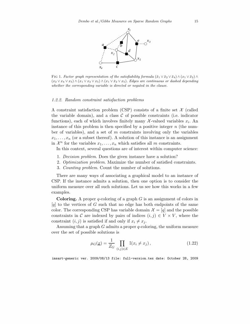
Fig 1. Factor graph representation of the satisfiability formula (x1 ∨ x2 ∨ x4)∧ (x1 ∨ x2)∧(x2 ∨ x4 ∨ x5)∧ (x1 ∨ x2 ∨ x5)∧ (x1 ∨ x2 ∨ x5). Edges are continuous or dashed dependingwhether the corresponding variable is directed or negated in the clause.

1.2.2. Random constraint satisfaction problems

A constraint satisfaction problem (CSP) consists of a finite set X (calledthe variable domain), and a class C of possible constraints (i.e. indicatorfunctions), each of which involves finitely many X -valued variables xi. Aninstance of this problem is then specified by a positive integer n (the num-ber of variables), and a set of m constraints involving only the variablesx1, . . . , xn (or a subset thereof). A solution of this instance is an assignmentin X n for the variables x1, . . . , xn which satisfies all m constraints.

In this context, several questions are of interest within computer science:

1. Decision problem. Does the given instance have a solution?2. Optimization problem. Maximize the number of satisfied constraints.3. Counting problem. Count the number of solutions.

There are many ways of associating a graphical model to an instance ofCSP. If the instance admits a solution, then one option is to consider theuniform measure over all such solutions. Let us see how this works in a fewexamples.

Coloring. A proper q-coloring of a graph G is an assignment of colors in[q] to the vertices of G such that no edge has both endpoints of the samecolor. The corresponding CSP has variable domain X = [q] and the possibleconstraints in C are indexed by pairs of indices (i, j) ∈ V × V , where theconstraint (i, j) is satisfied if and only if xi 6= xj .

Assuming that a graphG admits a proper q-coloring, the uniform measureover the set of possible solutions is

µG(x) =1

ZG

∏

(i,j)∈EI(xi 6= xj) , (1.22)



with ZG counting the number of proper q-colorings of G.

k-SAT. In case of k-satisfiability (in short, k-SAT), the variables arebinary xi ∈ X = 0, 1 and each constraint is of the form (xi(1), . . . , xi(k)) 6=(x∗i(1), . . . , x

∗i(k)) for some prescribed k-tuple (i(1), . . . , i(k)) of indices in V =

[n] and their prescribed values (x∗i(1), . . . , x∗i(k)). In this context constraints

are often referred to as ‘clauses’ and can be written as the disjunction (logicalOR) of k variables or their negations. The uniform measure over solutionsof an instance of this problem, if such solutions exist, is then

µ(x) =1

Z

m∏

a=1

I((xia(1), . . . , xia(k)) 6= (x∗ia(1), . . . , x

∗ia(k))

),

with Z counting the number of solutions. An instance can be associated to afactor graph, cf. Fig. 1. This is a bipartite graph having two types of nodes:variable nodes in V = [n] denoting the unknowns x1, . . . , xn and function(or factor) nodes in F = [m] denoting the specified constraints. Variablenode i and function node a are connected by an edge in the factor graph ifand only if variable xi appears in the a-th clause, so ∂a = ia(1), . . . , ia(k)and ∂i corresponds to the set of clauses in which i appears.

In general, such a construction associates to arbitrary CSP instance afactor graph G = (V, F,E). The uniform measure over solutions of such aninstance is then of the form

µG,ψ(x) =1

Z(G,ψ)

∏

a∈Fψa(x∂a) , (1.23)

for a suitable choice of ψ ≡ ψa(·) : a ∈ F. Such measures can also beviewed as the zero temperature limit of certain Boltzmann distributions.We note in passing that the probability measure of Eq. (1.4) corresponds tothe special case where all function nodes are of degree two.

1.2.3. Communications, estimation, detection

We describe next a canonical way of phrasing problems from mathematicalengineering in terms of graphical models. Though we do not detail it here,this approach applies to many specific cases of interest.

Let X1, . . . ,Xn be a collection of i.i.d. ‘hidden’ random variables with acommon distribution p0( · ) over a finite alphabet X . We want to estimatethese variables from a given collection of observations Y1, . . . , Ym. The a-thobservation (for a ∈ [m]) is a random function of the Xi’s for which i ∈ ∂a =



ia(1), . . . , ia(k). By this we mean that Ya is conditionally independent ofall the other variables given Xi : i ∈ ∂a and we write

P Ya ∈ A|X∂a = x∂a = Qa(A|x∂a) . (1.24)

for some probability kernel Qa( · | · ).The a posteriori distribution of the hidden variables given the observa-

tions is thus

µ(x|y) =1

Z(y)

m∏

a=1

Qa(ya|x∂a)n∏

i=1

p0(xi) . (1.25)

1.2.4. Graph and graph ensembles

The structure of the underlying graph G is of much relevance for the generalmeasures µG,ψ of (1.4). The same applies in the specific examples we haveoutlined in Section 1.2.

As already hinted, we focus here on (random) graphs that lack finitedimensional Euclidean structure. A few well known ensembles of such graphs(c.f. [54]) are:

I. Random graphs with a given degree distribution. Given a probabilitydistribution Pll≥0 over the non-negative integers, for each value ofn one draws the graph Gn uniformly at random from the collection ofall graphs with n vertices of which precisely ⌊nPk⌋ are of degree k ≥ 1(moving one vertex from degree k to k + 1 if needed for an even sumof degrees). We will denote this ensemble by G(P, n).

II. The ensemble of random k-regular graphs corresponds to Pk = 1 (withkn even). Equivalently, this is defined by the set of all graphs Gn overn vertices with degree k, endowed with the uniform measure. With aslight abuse of notation, we will denote it by G(k, n).

III. Erdos-Renyi graphs. This is the ensemble of all graphs Gn with nvertices and m = ⌊nα⌋ edges endowed with the uniform measure. Aslightly modified ensemble is the one in which each edge (i, j) is presentindependently with probability nα/

(n2

). We will denote it as G(α, n).

As further shown in Section 2.1, an important property of these graph en-sembles is that they converge locally to trees. Namely, for any integer ℓ, thedepth-ℓ neighborhood Bi(ℓ) of a uniformly chosen random vertex i convergesin distribution as n→ ∞ to a certain random tree of depth (at most) ℓ.



1.3. Detour: The Ising model on the integer lattice

In statistical physics it is most natural to consider models with local inter-actions on a finite dimensional integer lattice Z

d, where d = 2 and d = 3are often the physically relevant ones. While such models are of course non-mean field type, taking a short detour we next present a classical resultabout ferromagnetic Ising models on finite subsets of Z2.

Theorem 1.8. Let En,β denote expectations with respect to the ferromag-netic Ising measure (1.20) at zero magnetic field, in case G = (V,E) isa square grid of side

√n. Then, for large n the average magnetization

X = n−1∑ni=1Xi concentrates around zero for high temperature but not

for low temperature. More precisely, for some βo > 0,

limβ→∞

infn

En,β |X | = 1 , (1.26)

limn→∞ En,β |X |2 = 0 ∀β < βo . (1.27)

While this theorem and its proof refer to Z2, the techniques we use are

more general.Low temperature: Peierls argument. The proof of (1.26) is taken from[47] and based on the Peierls contour representation for the two dimensionalIsing model. We start off by reviewing this representation. First, given asquare grid G = (V,E) of side

√n in Z

2, for each (i, j) ∈ E draw a perpen-dicular edge of length one, centered at the midpoint of (i, j). Let E∗ denotethe collection of all these perpendicular edges and V ∗ the collection of theirend points, viewed as a finite subset of R2. A contour is a simple path onthe ‘dual’ graph G∗ = (V ∗, E∗), either closed or with both ends at boundary(i.e. degree one) vertices. A closed contour C divides V to two subsets, theinside of C and the outside of C. We further call as ‘inside’ the smallerof the two subsets into which a non-closed contour divides V (an arbitraryconvention can be used in case the latter two sets are of equal size). A Peierlscontours configuration (C, s) consists of a sign s ∈ +1,−1 and an edge-disjoint finite collection C of non-crossing contours (that is, whenever twocontours share a vertex, each of them bends there). Starting at an Ising con-figuration x ∈ Ω ≡ +1,−1V note that the set V+(x) = v ∈ V : xv = +1is separated from V−(x) = v ∈ V : xv = −1 by an edge-disjoint finitecollection C = C(x) of non-crossing contours. Further, it is not hard tocheck that the non-empty set U(x) = v ∈ V : v not inside any contourfrom C is either contained in V+(x), in which case s(x) = +1 or in V−(x),in which case s(x) = −1, partitioning Ω to Ω+ = x : s(x) = +1 and



Ω− = x : s(x) = −1. In the reverse direction, the Ising configuration isread off a Peierls contours configuration (C, s) by setting xv = s when thenumber of contours C ∈ C such that v ∈ V lies in the inside of C is evenwhile xv = −s when it is odd. The mapping x 7→ −x exchanges Ω+ with Ω−so

En,β[|X |] ≥ 2En,β[XI(X ∈ Ω+)] = 1 − 4

nEn,β[|V−(X)|I(X ∈ Ω+)] . (1.28)

If x is in Ω+ then |V−(x)| is bounded by the total number of vertices ofV inside contours of C, which by isoperimetric considerations is at most∑C∈C |C|2 (where |C| denotes the length of contour C). Further, our one-to-

one correspondence between Ising and Peierls contours configurations mapsthe Ising measure at β > 0 to uniform s ∈ +1,−1 independent of C whosedistribution is the Peierls measure

µ∗(C) =1

Z∗(β)

∏

C∈Ce−2β|C| .

Recall that if a given contour C is in some edge-disjoint finite collection C ofnon-crossing contours, then C′ = C\C is another such collection, with C 7→ C′

injective, from which we easily deduce that µ∗(C ∈ C) ≤ exp(−2β|C|) forany fixed contour C. Consequently,

En,β[|V−(X)|I(X ∈ Ω+)] ≤∑

C

|C|2µ∗(C ∈ C)

≤∑

ℓ≥2

ℓ2Nc(n, ℓ)e−2βℓ , (1.29)

where Nc(n, ℓ) denotes the number of contours of length ℓ for the squaregrid of side

√n. Each such contour is a length ℓ path of a non-reversing

nearest neighbor walk in Z2 starting at some point in V ∗. Hence, Nc(n, ℓ) ≤

|V ∗|3ℓ ≤ n3ℓ+1. Combining this bound with (1.28) and (1.29) we concludethat for all n,

En,β[|X |] ≥ 1 − 4

n

∑

ℓ≥2

ℓ2Nc(n, ℓ)e−2βℓ ≥ 1 − 12

∑

ℓ≥2

ℓ23ℓe−2βℓ .

We are thus done, as this lower bound converges to one for β → ∞.High-temperature expansion. The proof of (1.27), taken from [39], isby the method of high-temperature expansion which serves us again whendealing with the unfrustrated XORSAT model in Section 6.1. As in the



low-temperature case, the first step consists of finding an appropriate ‘ge-ometrical’ representation. To this end, given a subset U ⊆ V of vertices,let

ZU (β) =∑

x

xU expβ∑

(i,j)∈Exixj

and denote by G(U) the set of subgraphs of G having an odd-degree at eachvertex in U and an even degree at all other vertices. Then, with θ ≡ tanh(β)and F ⊆ E denoting both a subgraph of G and its set of edges, we claimthat

ZU (β) = 2|V |(cosh β)|E| ∑

F∈G(U)

θ|F | . (1.30)

Indeed, eβy = cosh(β)[1 + yθ] for y ∈ +1,−1, so by definition

ZU (β) = (cosh β)|E|∑

x

xU∏

(i,j)∈E[1 + xixjθ]

= (cosh β)|E| ∑

F⊆Eθ|F |∑

x

xU∏

(i,j)∈Fxixj .

By symmetry∑x xR is zero unless each v ∈ V appears in the set R an

even number of times, in which case the sum is 2|V |. In particular, the latterapplies for xR = xU

∏(i,j)∈F xixj if and only if F ∈ G(U) from which our

stated high-temperature expansion (1.30) follows.We next use this expansion to get a uniform in n decay of correlations at

all β < βo ≡ atanh(1/3), with an exponential rate with respect to the graphdistance d(i, j). More precisely, we claim that for any such β, n and i, j ∈ V

En,βXiXj ≤ (1 − 3θ)−1(3θ)d(i,j) . (1.31)

Indeed, from (1.30) we know that

En,βXiXj =Z(i,j)(β)

Z∅(β)=

∑F∈G(i,j) θ

|F |∑F ′∈G(∅) θ|F

′| .

Let F(i, j) denote the collection of all simple paths from i to j in Z2 and

for each such path Fi,j , denote by G(∅, Fi,j) the sub-collection of graphs inG(∅) that have no edge in common with Fi,j . The sum of vertex degreesin a connected component of a graph F is even, hence any F ∈ G(i, j)contains some path Fi,j ∈ F(i, j). Further, F is the edge-disjoint union of



Fi,j and F ′ = F \ Fi,j with F ′ having an even degree at each vertex. AsF ′ ∈ G(∅, Fi,j) we thus deduce that

En,βXiXj ≤∑

Fi,j∈F(i,j)

θ|Fi,j|∑F ′∈G(∅,Fi,j) θ

|F ′|∑F ′∈G(∅) θ|F

′| ≤∑

Fi,j∈F(i,j)

θ|Fi,j| .

The number of paths in F(i, j) of length ℓ is at most 3ℓ and their mini-mal length is d(i, j). Plugging this in the preceding bound establishes ourcorrelation decay bound (1.31).

We are done now, for there are at most 8d vertices in Z2 at distance d

from each i ∈ Z2. Hence,

En,β |X |2 =1

n2

∑

i,j∈VEn,βXiXj

≤ 1

n2(1 − 3θ)

∑

i,j∈V(3θ)d(i,j) ≤ 1

n(1 − 3θ)

∞∑

d=0

8d(3θ)d ,

which for θ < 1/3 decays to zero as n→ ∞.

2. Ising models on locally tree-like graphs

A ferromagnetic Ising model on the finite graph G (with vertex set V , andedge set E) is defined by the Boltzmann distribution µβ,B(x) of (1.20) withβ ≥ 0. In the following it is understood that, unless specified otherwise, themodel is ferromagnetic, and we will call it ‘Ising model on G.’

For sequences of graphs Gn = (Vn, En) of diverging size n, non-rigorousstatistical mechanics techniques, such as the ‘replica’ and ‘cavity methods,’make a number of predictions on this model when the graph G ‘lacks anyfinite-dimensional structure.’ The most basic quantity in this context is theasymptotic free entropy density, cf. Eq. (1.12),

φ(β,B) ≡ limn→∞

1

nlogZn(β,B) . (2.1)

The Curie-Weiss model, cf. Section 1.1, corresponds to the complete graphGn = Kn. Predictions exist for a much wider class of models and graphs,most notably, sparse random graphs with bounded average degree that arisein a number of problems from combinatorics and theoretical computer sci-ence (c.f. the examples of Section 1.2.2). An important new feature of sparsegraphs is that one can introduce a notion of distance between vertices as the



length of shortest path connecting them. Consequently, phase transitionsand coexistence can be studied with respect to the correlation decay proper-ties of the underlying measure. It turns out that this approach is particularlyfruitful and allows to characterize these phenomena in terms of appropriatefeatures of Gibbs measures on infinite trees. This direction is pursued in [58]in the case of random constraint satisfaction problems.

Statistical mechanics also provides methods for approximating the localmarginals of the Boltzmann measure of (1.20). Of particular interest is thealgorithm known in artificial intelligence and computer science under thename of belief propagation. Loosely speaking, this procedure consists of solv-ing by iteration certain mean field (cavity) equations. Belief propagation isshown in [29] to converge exponentially fast for an Ising model on any graph(even in a low-temperature regime lacking uniform decorrelation), with re-sulting asymptotically tight estimates for large locally tree-like graphs (seeSection 2.3).

2.1. Locally tree-like graphs and conditionally independent trees

We follow here [29], where the asymptotic free entropy density (2.1) is de-termined rigorously for certain sparse graph sequences Gn that convergelocally to trees. In order to make this notion more precise, we denote byBi(t) the subgraph induced by vertices of Gn whose distance from i is atmost t. Further, given two rooted trees T1 and T2 of the same size, we writeT1 ≃ T2 if T1 and T2 are identical upon labeling their vertices in a breadthfirst fashion following lexicographic order among siblings.

Definition 2.1. Let Pn denote the law of the ball Bi(t) when i ∈ Vn is auniformly chosen random vertex. We say that Gn converges locally to therandom rooted tree T if, for any finite t and any rooted tree T of depth atmost t,

limn→∞PnBi(t) ≃ T = PT(t) ≃ T , (2.2)

where T(t) denotes the subtree of first t generations of T.We also say that Gn is uniformly sparse if

liml→∞

lim supn→∞

1

|Vn|∑

i∈Vn

|∂i| I(|∂i| ≥ l) = 0 , (2.3)

where |∂i| denotes the size of the set ∂i of neighbors of i ∈ Vn (i.e. the degreeof i).



The proof that for locally tree-like graphs φn(β,B) = 1n logZn(β,B) con-

verges to (an explicit) limit φ(β,B) consists of two steps

(a). Reduce the computation of φn(β,B) to computing expectations oflocal (in Gn) quantities with respect to the Boltzmann measure (1.20).This is achieved by noting that the derivative of φn(β,B) with respectto β is a sum of such expectations.

(b). Show that under the Boltzmann measure (1.20) on Gn expectations oflocal quantities are, for t and n large, well approximated by the sameexpectations with respect to an Ising model on the associated randomtree T(t) (a philosophy related to that of [9]).

The key is of course step (b), and the challenge is to carry it out whenthe parameter β is large and we no longer have uniqueness of the Gibbsmeasure on the limiting tree T. Indeed, this is done in [29] for the followingcollection of trees of conditionally independent (and of bounded average)offspring numbers.

Definition 2.2. An infinite labeled tree T rooted at the vertex ø is calledconditionally independent if for each integer k ≥ 0, conditional on the sub-tree T(k) of the first k generations of T, the number of offspring ∆j forj ∈ ∂T(k) are independent of each other, where ∂T(k) denotes the set ofvertices at generation k. We further assume that the (conditional on T(k))first moments of ∆j are uniformly bounded by a given non-random finiteconstant ∆ and say that an unlabeled rooted tree T is conditionally inde-pendent if T ≃ T′ for some conditionally independent labeled rooted treeT′.

As shown in [29, Section 4] (see also Theorem 2.10), on such a tree, lo-cal expectations are insensitive to boundary conditions that stochasticallydominate the free boundary condition. Our program then follows by mono-tonicity arguments. An example of the monotonicity properties enjoyed bythe Ising model is provided by Lemma 2.12.

We next provide a few examples of well known random graph ensemblesthat are uniformly sparse and converge locally to conditionally indepen-dent trees. To this end, let P = Pk : k ≥ 0 be a probability distribu-tion over the non-negative integers, with finite, positive first moment P , setρk = (k + 1)Pk+1/P and denote its mean as ρ. We denote by T(ρ, t) therooted Galton-Watson tree of t ≥ 0 generations, i.e. the random tree suchthat each node has offspring distribution ρk, and the offspring numbersat different nodes are independent. Further, T(P, ρ, t) denotes the modifiedensemble where only the offspring distribution at the root is changed to



P . In particular, T(P, ρ,∞) is clearly conditionally independent. Other ex-amples of conditionally independent trees include: (a) deterministic treeswith bounded degree; (b) percolation clusters on such trees; (c) multi-typebranching processes.

When working with random graph ensembles, it is often convenient towork with the configuration models [17] defined as follows. In the case ofthe Erdos-Renyi random graph, one draws m i.i.d. edges by choosing theirendpoints ia, ja independently and uniformly at random for a = 1, . . . ,m.For a graph with given degree distribution Pk, one first partitions thevertex sets into subsets V0, of ⌊nP0⌋ vertices, V1 of ⌊nP1⌋ vertices, V2 of ⌊nP2⌋vertices, etc. Then associate k half-edges to the vertices in Vk for each k(eventually adding one half edge to the last node, to make their total numbereven). Finally, recursively match two uniformly random half edges until thereis no unmatched one. Whenever we need to make the distinction we denoteby P∗( · ) probabilities under the corresponding configuration model.

The following simple observation transfers results from configuration mod-els to the associated uniform models.

Lemma 2.3. Let An be a sequence of events, such that, under the configu-ration model

∑

n

P∗(Gn 6∈ An) <∞ . (2.4)

Further, assume m = ⌊αn⌋ with α fixed (for Erdos-Renyi random graphs),or Pk fixed, with bounded first moment (for general degree distribution).Then, almost surely under the uniform model, property An holds for all nlarge enough.

Proof. The point is that, the graph chosen under the configuration model isdistributed uniformly when further conditional on the property Ln that ithas neither self-loops nor double edges (see [54]). Consequently,

P(Gn 6∈ An) = P∗(Gn 6∈ An|Ln) ≤ P∗(Gn 6∈ An)/P∗(Ln) .

The thesis follows by recalling that P∗(Ln) is bounded away from 0 uniformlyin n for the models described here (c.f. [54]), and applying the Borel-Cantellilemma.

Our next lemma ensures that we only need to check the local (weak)convergence in expectation with respect to the configuration model.



Lemma 2.4. Given a finite rooted tree T of at most t generations, assumethat

limn→∞P∗Bi(t) ≃ T = QT , (2.5)

for a uniformly random vertex i ∈ Gn. Then, under both the configurationand the uniform models of Lemma 2.3, PnBi(t) ≃ T → QT almost surely.

Proof. Per given value of n consider the random variable Z ≡ PnBi(t) ≃T. In view of Lemma 2.3 and the assumption (2.5) that E∗[Z] = P∗Bi(t) ≃T converges to QT , it suffices to show that P∗|Z−E∗[Z]| ≥ δ is summable(in n), for any fixed δ > 0. To this end, let r denote the maximal degreeof T . The presence of an edge (j, k) in the resulting multi-graph Gn affectsthe event Bi(t) ≃ T only if there exists a path of length at most t in Gnbetween i and j, k, the maximal degree along which is at most r. Per givenchoice of (j, k) there are at most u = u(r, t) ≡ 2

∑tl=0 r

l such values of i ∈ [n],hence the Lipschitz norm of Z as a function of the location of the m edgesof Gn is bounded by 2u/n. Let Gn(t) denote the graph formed by the first tedges (so Gn(m) = Gn), and introduce the martingale Z(t) = E∗[Z|Gn(t)],so Z(m) = Z and Z(0) = E∗[Z]. A standard argument (c.f. [10, 81]), showsthat the conditional laws P∗( · |Gn(t)) and P∗( · |Gn(t + 1)) of Gn can becoupled in such a way that the resulting two (conditional) realizations ofGn differ by at most two edges. Consequently, applying Azuma-Hoeffdinginequality we deduce that for any T , M and δ > 0, some c0 = c0(δ,M, u)positive and all m ≤ nM ,

P∗(∣∣Z − E∗[Z]

∣∣ ≥ δ) = P∗(∣∣Zm − Z0

∣∣ ≥ δ) ≤ 2e−c0n , (2.6)

which is more than enough for completing the proof.

Proposition 2.5. Given a distribution Pll≥0 of finite mean, let Gnn≥1

be a sequence of graphs whereby Gn is distributed according to the ensembleG(P, n) with degree distribution P . Then the sequence Gn is almost surelyuniformly sparse and converges locally to T(P, ρ,∞).

Proof. Note that for any random graph Gn of degree distribution P ,

En(l) ≡∑

i∈Vn

|∂i| I(|∂i| ≥ l) ≤ 1 + n∑

k≥lkPk ≡ 1 + nP l . (2.7)

Our assumption that P =∑k kPk is finite implies that P l → 0 as l → ∞,

so any such sequence of graphs Gn is uniformly sparse.



As the collection of finite rooted trees of finite depth is countable, byLemma 2.4 we have the almost sure local convergence of Gn to T(P, ρ,∞)once we show that P∗(Bi(t) ≃ T ) → P(T(P, ρ, t) ≃ T ) as n → ∞, wherei ∈ Gn is a uniformly random vertex and T is any fixed finite, rooted treeof at most t generations.

To this end, we opt to describe the distribution of Bi(t) under the config-uration model as follows. First fix a non-random partition of [n] to subsetsVk with |Vk| = ⌊nPk⌋, and assign k half-edges to each vertex in Vk. Then,draw a uniformly random vertex i ∈ [n]. Assume it is in Vk, i.e. has khalf-edges. Declare these half-edges ‘active’. Recursively sample k unpaired(possibly active) half-edges, and pair the active half-edges to them. Repeatthis procedure for the vertices thus connected to i and proceed in a breadthfirst fashion for t generations (i.e. until all edges of Bi(t) are determined).Consider now the modified procedure in which, each time an half-edge isselected, the corresponding vertex is put in a separate list, and replaced bya new one with the same number of half-edges, in the graph. Half-edges inthe separate list are active, but they are not among the candidates in thesampling part. This modification yields Bi(t) which is a random tree, specifi-

cally, an instance of T(P (n), ρ(n), t), where P(n)k = ⌊nPk⌋/

∑l⌊nPl⌋. Clearly,

T(P (n), ρ(n), t) converges in distribution as n→ ∞ to T(P, ρ, t). The proof isthus complete by providing a coupling in which the probability that eitherBi(t) ≃ T under the modified procedure and Bi(t) 6≃ T under the originalprocedure (i.e. the configurational model), or vice versa, is at most 4|T |2/n.Indeed, after ℓ steps, a new vertex j is sampled by the pairing with prob-ability pj ∝ kj(ℓ) in the original procedure and p′j ∝ kj(0) in the modifiedone, where kj(ℓ) is the number of free half-edges associated to vertex j atstep ℓ. Having to consider at most |T | steps and stopping once the originaland modified samples differ, we get the stated coupling upon noting that||p − p′||TV ≤ 2|T |/n (as both samples must then be subsets of the giventree T ).

Proposition 2.6. Let Gnn≥1 be a sequence of Erdos-Renyi random graphs,i.e. of graphs drawn either from the ensemble G(α, n) or from the uniformmodel with m = m(n) edges, where m(n)/n → α. Then, the sequence Gn isalmost surely uniformly sparse and converges locally to the Galton-Watsontree T(P, ρ,∞) with Poisson(2α) offspring distribution P (in which caseρk = Pk).

Proof. We denote by P〈m〉(·) and E〈m〉(·) the probabilities and expectationswith respect to a random graph Gn chosen uniformly from the ensemble of



all graphs of m edges, with P〈m〉∗ (·) and E

〈m〉∗ (·) in use for the corresponding

configuration model.We start by proving the almost sure uniform sparsity for graphs Gn from

the uniform ensemble ofm = m(n) edges providedm(n)/n ≤M for all n andsome finiteM . To this end, by Lemma 2.3 it suffices to prove this property forthe corresponding configuration model. Setting Z ≡ n−1En(l) for En(l) of(2.7) and P 〈m〉 to be the Binomial(2m, 1/n) distribution of the degree of each

vertex of Gn in this configuration model, note that E〈m〉∗ [Z] = P

〈m〉l ≤ P l

for P l ≡∑k≥l kPk of the Poisson(4M) degree distribution P , any n ≥ 2

and m ≤ nM . Since∑k kPk is finite, necessarily P l → 0 as l → ∞ and the

claimed almost sure uniform sparsity follows from the summability in n, per

fixed l and δ > 0 of P〈m〉∗ Z − E

〈m〉∗ [Z] ≥ δ, uniformly in m ≤ nM . Recall

that the presence of an edge (j, k) in the resulting multi-graph Gn changesthe value of En(l) by at most 2l, hence the Lipschitz norm of Z as a functionof the location of the m edges of Gn is bounded by 2l/n. Thus, applyingthe Azuma-Hoeffding inequality along the lines of the proof of Lemma 2.4we get here a uniform in m ≤ nM and summable in n bound of the form of(2.6).

As argued in proving Proposition 2.5, by Lemma 2.4 we further have theclaimed almost sure local convergence of graphs from the uniform ensembles

of m = m(n) edges, once we verify that (2.5) holds for P〈m〉∗ (·) and QT =

PT(P, ρ, t) ≃ T with the Poisson(2α) offspring distribution P . To this end,fix a finite rooted tree T of depth at most t and order its vertices from 1(for ø) to |T | in a breadth first fashion following lexicographic order amongsiblings. Let ∆v denote the number of offspring of v ∈ T with T (t− 1) thesub-tree of vertices within distance t− 1 from the root of T (so ∆v = 0 forv /∈ T (t − 1)), and denoting by b ≡ ∑

v≤T (t−1) ∆v = |T | − 1 the number ofedges of T . Under our equivalence relation between trees there are

b∏

v=1

n− v

∆v!

distinct embeddings of T in [n] for which the root of T is mapped to 1.Fixing such an embedding, the event B1(t) ≃ T specifies the b edges inthe restriction of En to the vertices of T and further forbids having any edgein En between T (t−1) and a vertex outside T . Thus, under the configuration

model P〈m〉∗ (·) with m edges chosen with replacement uniformly among the

n2 ≡ (n2

)possible edges, the event B1(t) ≃ T occurs per such an embedding

for precisely (n2 − a− b)m−bm!/(m− b)! of the nm2 possible edge selections,



where a = (n − |T |)|T (t − 1)| + (b2

). With P

〈m〉∗ (Bi(t) ≃ T ) independent of

i ∈ [n], it follows that

P〈m〉∗ (Bi(t) ≃ T ) =

2bm!

nb(m− b)!

(1 − a+ b

n2

)m−b b∏

v=1

n− v

(n− 1)∆v !.

Since b is independent of n and a = n|T (t− 1)| + O(1), it is easy to verifythat for n→ ∞ and m/n→ α the latter expression converges to

QT ≡ (2α)be−2α|T (t−1)|b∏

v=1

1

∆v!=

|T (t−1)|∏

v=1

P∆v = PT(P, ρ, t) ≃ T

(where Pk = (2α)ke−2α/k!, hence ρk = Pk for all k). Further, fixing γ < 1and denoting by In the interval of width 2nγ around αn, it is not hard to

check that P〈m〉∗ (Bi(t) ≃ T ) → QT uniformly over m ∈ In.

Let P(n)(·) and E(n)(·) denote the corresponding laws and expectationswith respect to random graphs Gn from the ensembles G(α, n), i.e. whereeach edge is chosen independently with probability qn = 2α/(n − 1). Thepreceding almost sure local convergence and uniform sparseness extend tothese graphs since each law P(n)(·) is a mixture of the laws P〈m〉(·),m =1, 2, . . . with mixture coefficients P(n)(|En| = m) that are concentrated onm ∈ In. Indeed, by the same argument as in the proof of Lemma 2.3, forany sequence of events An,

P(n)(Gn /∈ An) ≤ P(n)(|En| /∈ In) + η−1 supm∈In

P〈m〉∗ (Gn /∈ An) , (2.8)

whereη = lim inf

n→∞ infm∈In

P〈m〉∗ (Ln) ,

is strictly positive (c.f. [54]). Under P(n)(·) the random variable |En| has theBinomial(n(n − 1)/2, qn) distribution (of mean αn). Hence, upon applyingMarkov’s inequality, we find that for some finite c1 = c1(α) and all n,

P(n)(|En| /∈ In) ≤ n−4γ E(n)[(|En| − αn)4] ≤ c1n2−4γ ,

so taking γ > 3/4 guarantees the summability (in n), of P(n)(|En| /∈ In). For

given δ > 0 we already proved the summability in n of supm∈In P〈m〉∗ (Gn /∈

An) both for An = n−1En(l) < P l + δ and for An = |Pn(Bi(t) ≃T ) − QT | < 2δ. In view of this, considering (2.8) for the former choice ofAn yields the almost sure uniform sparsity of Erdos-Renyi random graphs



from G(α, n), while the latter choice of An yields the almost sure local con-vergence of these random graphs to the Galton-Watson tree T(P, ρ,∞) withPoisson(2α) offspring distribution.

Remark 2.7. As a special case of Proposition 2.5, almost every sequenceof uniformly random k-regular graphs of n vertices converges locally to the(non-random) rooted k-regular infinite tree Tk(∞).

Let Tk(ℓ) denote the tree induced by the first ℓ generations of Tk(∞), i.e.Tk(0) = ø and for ℓ ≥ 1 the tree Tk(ℓ) has k offspring at ø and (k − 1)offspring for each vertex at generations 1 to ℓ−1. It is easy to check that forany k ≥ 3, the sequence of finite trees Tk(ℓ)ℓ≥0 does not converge locallyto Tk(∞). Instead, it converges to the following random k-canopy tree (c.f.[7] for a closely related definition).

Lemma 2.8. For any k ≥ 3, the sequence of finite trees Tk(ℓ)ℓ≥0 con-verges locally to the k-canopy tree. This random infinite tree, denoted CTk, isformed by the union of the infinite ray ~R ≡ (r, r+1), r ≥ 0 and additionalfinite trees Tk−1(r), r ≥ 0 such that Tk−1(r) is rooted at the r-th vertexalong ~R. The root of CTk is on ~R with P(CTk rooted at r) = (k−2)/(k−1)r+1

for r ≥ 0.

Proof. This local convergence is immediate upon noting that there are ex-actly nr = k(k− 1)r−1 vertices at generation r ≥ 1 of Tk(ℓ), hence |Tk(ℓ)| =[k(k − 1)ℓ − 2]/(k − 2) and nℓ−r/|Tk(ℓ)| → P(CTk rooted at r) as ℓ → ∞,for each fixed r ≥ 0 and k ≥ 3 (and Bi(ℓ) matches for each i of generationℓ− r in Tk(ℓ) the ball Br(ℓ) of the k-canopy tree).

Remark 2.9. Note that the k-canopy tree is not conditionally independent.

2.2. Ising models on conditionally independent trees

Following [29] it is convenient to extend the model (1.20) by allowing forvertex-dependent magnetic fields Bi, i.e. to consider

µ(x) =1

Z(β,B)exp

β∑

(i,j)∈Exixj +

∑

i∈VBixi

. (2.9)

In this general context, it is possible to prove correlation decay results forIsing models on conditionally independent trees. Beyond their independentinterest, such results play a crucial role in our analysis of models on sparsegraph sequences.



To state these results denote by µℓ,0 the Ising model (2.9) on T(ℓ) withmagnetic fields Bi (also called free boundary conditions), and by µℓ,+ themodified Ising model corresponding to the limit Bi ↑ +∞ for all i ∈ ∂T(ℓ)(also called plus boundary conditions), using µℓ for statements that applyto both free and plus boundary conditions.

Theorem 2.10. Suppose T is a conditionally independent infinite tree of

average offspring numbers bounded by ∆, as in Definition 2.2. Let 〈 · 〉(r)idenote the expectation with respect to the Ising distribution on the subtree of iand all its descendants in T(r) and 〈x; y〉 ≡ 〈xy〉−〈x〉〈y〉 denotes the centeredtwo point correlation function. There exist A finite and λ positive, dependingonly on 0 < Bmin ≤ Bmax, βmax and ∆ finite, such that if Bi ≤ Bmax forall i ∈ T(r − 1) and Bi ≥ Bmin for all i ∈ T(ℓ), then for any r ≤ ℓ andβ ≤ βmax,

E ∑

i∈∂T(r)

〈xø;xi〉(ℓ)ø

≤ Ae−λr . (2.10)

If in addition Bi ≤ Bmax for all i ∈ T(ℓ−1) then for some C = C(βmax, Bmax)finite

E ||µℓ,+T(r) − µℓ,0

T(r)||TV ≤ Ae−λ(ℓ−r) EC |T(r)| . (2.11)

The proof of this theorem, given in [29, Section 4], relies on monotonicityproperties of the Ising measure, and in particular on the following classicalinequality.

Proposition 2.11 (Griffiths inequalities). Given a finite set V and param-eters J = (JR, R ⊆ V ) with JR ≥ 0, consider the extended ferromagneticIsing measure

µJ(x) =1

Z(J)exp

∑

R⊆VJRxR

, (2.12)

where x ∈ +1,−1V and xR ≡ ∏u∈R xu. Then, for X of law µJ and any

A,B ⊆ V ,

EJ [XA] =1

Z(J)

∑

x

xA exp ∑

R⊆VJRxR

≥ 0 , (2.13)

∂

∂JBEJ [XA] = CovJ(XA,XB) ≥ 0 . (2.14)



Proof. See [61, Theorem IV.1.21] (and consult [44] for generalizations ofthis result).

Note that the measure µ(·) of (2.9) is a special case of µJ (taking Ji =Bi, Ji,j = β for all (i, j) ∈ E and JR = 0 for all other subsets of V ). Thus,Griffiths inequalities allow us to compare certain marginals of the lattermeasure for a graph G and non-negative β, Bi with those for other choicesof G, β and Bi. To demonstrate this, we state (and prove) the following wellknown general comparison results.

Lemma 2.12. Fixing β ≥ 0 and Bi ≥ 0, for any finite graph G = (V,E) andA ⊆ V let 〈xA〉G = µ(xA = 1) − µ(xA = −1) denote the mean of xA underthe corresponding Ising measure on G. Similarly, for U ⊆ V let 〈xA〉0U and〈xA〉+U denote the magnetization induced by the Ising measure subject to free(i.e. xu = 0) and plus (i.e. xu = +1) boundary conditions, respectively, at allu /∈ U . Then, 〈xA〉0U ≤ 〈xA〉G ≤ 〈xA〉+U for any A ⊆ U . Further, U 7→ 〈xA〉0Uis monotone non-decreasing and U 7→ 〈xA〉+U is monotone non-increasing,both with respect to set inclusion (among sets U that contain A).

Proof. From Griffiths inequalities we know that J 7→ EJ [XA] is monotone

non-decreasing (where J ≥ J if and only if JR ≥ JR for all R ⊆ V ). Further,〈xA〉G = EJ0 [XA] where J0

i = Bi, J0i,j = β when (i, j) ∈ E and all other

values of J0 are zero. Considering

Jη,UR = J0R + ηI(R ⊆ U c, |R| = 1) ,

with η 7→ Jη,U non-decreasing, so is η 7→ EJη,U [XA]. In addition, µJη,U (xu =

−1) ≤ C e−2η whenever u /∈ U . Hence, as η ↑ ∞ the measure µJη,U convergesto µJ subject to plus boundary conditions xu = +1 for u /∈ U . Consequently,

〈xA〉G ≤ EJη,U [XA] ↑ 〈xA〉+U .

Similarly, let JUR = J0RI(R ⊆ U) noting that under µJU the random vector

xU is distributed according to the Ising measure µ restricted to GU (alter-natively, having free boundary conditions xu = 0 for u /∈ U). With A ⊆ Uwe thus deduce that

〈xA〉0U = EJU [XA] ≤ EJ0 [XA] = 〈xA〉G .

Finally, the stated monotonicity of U 7→ 〈xA〉0U and U 7→ 〈xA〉+U are in viewof Griffiths inequalities the direct consequence of the monotonicity (withrespect to set inclusions) of U 7→ JU and U 7→ Jη,U , respectively.



In addition to Griffiths inequalities, the proof of Theorem 2.10 uses alsothe GHS inequality [48] which regards the effect of a magnetic field B onthe local magnetizations at various vertices. It further uses an extension ofSimon’s inequality (about the centered two point correlation functions inferromagnetic Ising models with zero magnetic field, see [82, Theorem 2.1]),to arbitrary magnetic field, in the case of Ising models on trees. Namely,[29, Lemma 4.3] states that if edge (i, j) is on the unique path from ø tok ∈ T(ℓ), with j a descendant of i ∈ ∂T(t), t ≥ 0, then

〈xø;xk〉(ℓ)ø ≤ cosh2(2β +Bi) 〈xø;xi〉(t)ø 〈xj ;xk〉(ℓ)j . (2.15)

2.3. Algorithmic implications: belief propagation

The ‘belief propagation’ (BP) algorithm consists of solving by iterations acollection of Bethe-Peierls (or cavity) mean field equations. More precisely,for the Ising model (1.20) we associate to each directed edge in the graph i→j, with (i, j) ∈ G, a distribution (or ‘message’) νi→j(xi) over xi ∈ +1,−1,using then the following update rule

ν(t+1)i→j (xi) =

1

z(t)i→j

eBxi∏

l∈∂i\j

∑

xl

eβxixlν(t)l→i(xl) (2.16)

starting at a positive initial condition, namely where ν(0)i→j(+1) ≥ ν

(0)i→j(−1)

at each directed edge.Applying Theorem 2.10 we establish in [29, Section 5] the uniform expo-

nential convergence of the BP iteration to the same fixed point of (2.16),irrespective of its positive initial condition. As we further show there, fortree-like graphs the limit of the BP iteration accurately approximates localmarginals of the Boltzmann measure (1.20).

Theorem 2.13. Assume β ≥ 0, B > 0 and G is a graph of finite maximaldegree ∆. Then, there exists A = A(β,B,∆) and c = c(β,B,∆) finite,λ = λ(β,B,∆) > 0 and a fixed point ν∗i→j of the BP iteration (2.16) such

that for any positive initial condition ν(0)l→k and all t ≥ 0,

sup(i,j)∈E

‖ν(t)i→j − ν∗i→j‖TV ≤ A exp(−λt) . (2.17)

Further, for any io ∈ V , if Bio(t) is a tree then for U ≡ Bio(r)

||µU − νU ||TV ≤ expcr+1 − λ(t− r)

, (2.18)



where µU ( · ) is the law of xU ≡ xi : i ∈ U under the Ising model (1.20)and νU the probability distribution

νU (xU ) =1

zUexp

β

∑

(i,j)∈EU

xixj +B∑

i∈U\∂Uxi ∏

i∈∂Uν∗i→j(i)(xi) , (2.19)

with EU the edge set of U whose border is ∂U (i.e. the set of its vertices atdistance r from io), and j(i) is any fixed neighbor in U of i.

2.4. Free entropy density, from trees to graphs

Bethe-Peierls approximation (we refer to Section 3.1 for a general introduc-tion), allows us to predict the asymptotic free entropy density for sequencesof graphs that converge locally to conditionally independent trees. We startby explaining this prediction in a general setting, then state a rigorous resultwhich verifies it for a specific family of graph sequences.

To be definite, assume that B > 0. Given a graph sequence Gn thatconverges to a conditionally independent tree T with bounded average off-spring number, let L = ∆ø be the degree of its root. Define the ’cavity fields’

h1, . . . , hL by letting hj = limt→∞ h(t)j with h

(t)j ≡ atanh[〈xj〉(t)j ], where

〈 · 〉(t)j denotes expectation with respect to the Ising distribution on the sub-tree induced by j ∈ ∂ø and all its descendants in T(t) (with free boundary

conditions). We note in passing that t 7→ h(t)j is stochastically monotone

(and hence has a limit in law) by Lemma 2.12. Further h1, . . . , hL areconditionally independent given L. Finally, define θ = tanh(β) and

h−j = B +L∑

k=1,k 6=jatanh[θ tanh(hk)] . (2.20)

The Bethe-Peierls free energy density is given by

ϕ(β,B) ≡ 1

2ELγ(θ) − 1

2E L∑

j=1

log[1 + θ tanh(h−j) tanh(hj)]

+ E logeB

L∏

j=1

[1 + θ tanh(hj)] + e−BL∏

j=1

[1 − θ tanh(hj)], (2.21)

for γ(u) = −12 log(1 − u2). We refer to Section 3.3 where this formula is

obtained as a special case of the general expression for a Bethe-Peierls free



energy. The prediction is extended to B < 0 by letting ϕ(β,B) = ϕ(β,−B),and to B = 0 by letting ϕ(β, 0) be the limit of ϕ(β,B) as B → 0.

As shown in [29, Lemma 2.2], when T = T(P, ρ,∞) is a Galton-Watsontree, the random variables hj have a more explicit characterization interms of the following fixed point distribution.

Lemma 2.14. In case T = T(P, ρ,∞) consider the random variables h(t)where h(0) ≡ 0 and for t ≥ 0,

h(t+1) d= B +

K∑

i=1

atanh[θ tanh(h(t)i )] , (2.22)

with h(t)i i.i.d. copies of h(t) that are independent of the variable K of dis-

tribution ρ. If B > 0 and ρ < ∞ then t 7→ h(t) is stochastically monotone(i.e. there exists a coupling under which P(h(t) ≤ h(t+1)) = 1 for all t), andconverges in law to the unique fixed point h∗ of (2.22) that is supported on[0,∞). In this case, hj of (2.21) are i.i.d. copies of h∗ that are independentof L.

The main result of [29] confirms the statistical physics prediction for thefree entropy density.

Theorem 2.15. If ρ is finite then for any B ∈ R, β ≥ 0 and sequenceGnn∈N of uniformly sparse graphs that converges locally to T(P, ρ,∞),

limn→∞

1

nlogZn(β,B) = ϕ(β,B) . (2.23)

We proceed to sketch the outline of the proof of Theorem 2.15. For uni-formly sparse graphs that converge locally to T(P, ρ,∞) the model (1.20)has a line of first order phase transitions for B = 0 and β > βc (that is, wherethe continuous function B 7→ ϕ(β,B) exhibits a discontinuous derivative).Thus, the main idea is to utilize the magnetic field B to explicitly break the+/− symmetry, and to carefully exploit the monotonicity properties of theferromagnetic Ising model in order to establish the result even at β > βc.

Indeed, since φn(β,B) ≡ 1n logZn(β,B) is invariant under B → −B and

is uniformly (in n) Lipschitz continuous in B with Lipschitz constant one,for proving the theorem it suffices to fix B > 0 and show that φn(β,B)converges as n → ∞ to the predicted expression ϕ(β,B) of (2.21). This isobviously true for β = 0 since φn(0, B) = log(2 coshB) = ϕ(0, B). Next,denoting by 〈 · 〉n the expectation with respect to the Ising measure on Gn



(at parameters β and B), it is easy to see that

∂βφn(β,B) =1

n

∑

(i,j)∈En

〈xixj〉n =1

2En

[ ∑

j∈∂i〈xixj〉n

]. (2.24)

With |∂βφn(β,B)| ≤ |En|/n bounded by the assumed uniform sparsity, it isthus enough to show that the expression in (2.24) converges to the partialderivative of ϕ(β,B) with respect to β. Turning to compute the latter deriva-tive, after a bit of real analysis we find that the dependence of hj , h−j onβ can be ignored (c.f. [29, Corollary 6.3] for the proof of this fact in caseT = T(P, ρ,∞)). That is, hereafter we simply compute the partial derivativein β of the expression (2.21) while considering the law of hj and h−j tobe independent of β. To this end, setting zj = tanh(hj) and yj = tanh(h−j),the relation (2.20) amounts to

yj =eB∏k 6=j(1 + θzk) − e−B

∏k 6=j(1 − θzk)

eB∏k 6=j(1 + θzk) + e−B

∏k 6=j(1 − θzk)

for which it follows that

∂

∂θ

l∑

j=1

log(1 + θzjyj)

=∂

∂θlog

eB

l∏

j=1

(1 + θzj) + e−Bl∏

j=1

(1 − θzj)

=l∑

j=1

zjyj1 + θzjyj

and hence a direct computation of the derivative in (2.21) leads to

∂β ϕ(β,B) =1

2E[ ∑

j∈∂ø

〈xøxj〉T], (2.25)

where 〈·〉T denotes the expectation with respect to the Ising model

µT(xø, x1, . . . , xL) =1

zexp

β

L∑

j=1

xøxj +Bxø +L∑

j=1

hjxj, (2.26)

on the ‘star’ T(1) rooted at ø and the random cavity fields hj of (2.21).In comparison, fixing a positive integer t and considering Lemma 2.12

for A ≡ i, j and U ≡ Bi(t), we find that the correlation 〈xixj〉n liesbetween the correlations 〈xixj〉0Bi(t)

and 〈xixj〉+Bi(t)for the Ising model on



the subgraph Bi(t) with free and plus, respectively, boundary conditions at∂Bi(t). Thus, in view of (2.24)

1

2EnF0(Bi(t)) ≤ ∂β φn(β,B) ≤ 1

2EnF+(Bi(t)) ,

where F0/+(Bi(t)) ≡∑j∈∂i〈xixj〉0/+Bi(t)

.Next, taking n → ∞ we rely on the following consequence of the local

convergence of a uniformly sparse graph sequence Gn (c.f. [29, Lemma6.4] for the derivation of a similar result).

Lemma 2.16. Suppose a uniformly sparse graph sequence Gn convergeslocally to the random tree T. Fix an integer t ≥ 0 and a function F (·)on the collection of all possible subgraphs that may occur as Bi(t), suchthat F (Bi(t))/(|∂i| + 1) is uniformly bounded and F (T1) = F (T2) wheneverT1 ≃ T2. Then,

limn→∞EnF (Bi(t)) = EF (T(t)) . (2.27)

Indeed, applying this lemma for the functions F0(·) and F+(·) we findthat

1

2EF0(T(t)) ≤ lim inf

n→∞ ∂β φn(β,B) ≤ lim supn→∞

∂β φn(β,B) ≤ 1

2EF+(T(t)) .

To compute F0/+(T(t)) we first sum over the values of xk for k ∈ T(t)\T(1).This has the effect of reducing F0/+(T(t)) to the form of

∑j∈∂ø〈xøxj〉T and

the cavity fields are taken as h(t),0/+j ≡ atanh[〈xj〉(t),0/+j ]. Further, from

(2.11) we deduce that as t→ ∞ both sets of cavity fields converge in law tothe same limit hj. Since E[〈xøxj〉T] are continuous with respect to suchconvergence in law, we get by (2.25) that

limt→∞

1

2EF0/+(T(t)) = ∂β ϕ(β,B) ,

which completes the proof of the theorem.

2.5. Coexistence at low temperature

We focus here on the ferromagnetic Ising model on a random k-regulargraph with k ≥ 3 and zero magnetic field. In order to simplify derivations,it is convenient to use the so-called configuration model for random regulargraphs [17]. A graph from this ensemble is generated by associating k half



edges to each i ∈ [n] (with kn even) and pairing them uniformly at random.In other words, the collection En of m ≡ kn/2 edges is obtained by pairingthe kn half-edges. Notice that the resulting object is in fact a multi-graphi.e. it might include double edges and self-loops. However the number of such‘defects’ is O(1) as n → ∞ and hence the resulting random graph modelshares many properties with random k-regular graphs. With a slight abuseof notation, we keep denoting by G(k, n) the multi-graph ensemble.

For β ≥ 0 we consider the distribution

µn,β,k(x) =1

Z(Gn)exp

β

∑

(i,j)∈En

xixj. (2.28)

Recall Remark 2.7 that any sequence of random graphs Gn from theensembles G(k, n) is almost surely uniformly sparse and converges locally tothe infinite k-regular tree. Thus, considering the function

ϕk(β, h) ≡k

2

γ(θ) − log[1 + θ tanh2(h)]

+ log[1 + θ tanh(h)]k + [1 − θ tanh(h)]k

,

of h ∈ R and θ = tanh(β), we have from Theorem 2.15 that

limn→∞

1

nlogZ(Gn) = ϕk(β, h

∗) , (2.29)

where the cavity field h∗ is the largest solution of

g(h) ≡ (k − 1)atanh[θ tanh(h)] − h = 0 . (2.30)

Indeed, the expression for ϕk(β, h∗) is taken from (2.21), noting that here

L = K+1 = k is non-random, hence so are h−j = hj = h∗. It is not hard tocheck by calculus that the limit as B ↓ 0 of the unique positive solution ofg(h) = −B is strictly positive if and only if β > βc ≡ atanh(1/(k − 1)), inwhich case g(−h) = −g(h) is zero if and only if h ∈ 0,±h∗ with g′(0) > 0and g′(h∗) < 0 (c.f. [64]).

We expect coexistence in this model if and only if β > βc (where wehave a line of first order phase transitions for the asymptotic free entropyat B = 0), and shall next prove the ‘if’ part.

Theorem 2.17. With probability one, the ferromagnetic Ising measuresµn,β,k on uniformly random k-regular multi-graphs from the ensemble G(k, n)exhibit coexistence if (k − 1) tanh(β) > 1.



Proof. As in the proof of Theorem 1.5 (for the Curie-Weiss model), weagain consider the partition of X n to Ω+ ≡ x :

∑i xi ≥ 0 and Ω− ≡

x :∑i xi < 0. From the invariance of µn,β,k with respect to the sign

change x 7→ −x it follows that µn,β,k(Ω+) = µn,β,k(Ω0) + µn,β,k(Ω−) whereΩr ≡ x :

∑i xi = r. Hence, to prove coexistence it suffices to show that

for ǫ > 0 small enough, with probability one

lim supn→∞

1

nlog

∑

|r|≤nǫµn,β,k(Ωr)

< 0 . (2.31)

To this end, note that µn,β,k(Ωr) = Zr(Gn)/Z(Gn) for the restricted partitionfunction

Zr(Gn) ≡∑

x∈Ωr

expβ

∑

(i,j)∈En

xixj. (2.32)

Further, recall that by Markov’s inequality and the Borel-Cantelli lemma,for any positive random variables Yn, with probability one

lim supn→∞

1

nlog Yn ≤ lim sup

n→∞1

nlog E(Yn) .

Thus, combining (2.29) with the latter inequality for Yn =∑

|r|≤nǫZr(Gn)we arrive at the inequality (2.31) upon proving the following lemma (c.f. [43,Section 5]).

Lemma 2.18. Considering even values of n and assuming β > βc, we havethat

limǫ→0

lim supn→∞

1

nlog

∑

|r|≤nǫEZr(Gn)

= ϕk(β, 0) < ϕk(β, h

∗) . (2.33)

Proof. First, following the calculus preceding (2.25) we get after some alge-braic manipulations that

∂hϕk(β, h) =kθ

cosh2(h)[f(tanh(u), c) − f(tanh(h), c)]

for c = c(h) ≡ θ tanh(h) and u = u(h) ≡ (k − 1)atanh(c), where for c ≥ 0the function f(x, c) = x/(1 + cx) is monotone increasing in x ≥ 0. Withβ > βc we know already that g(h) > 0 (for g(·) of (2.30)), hence u(h) > hfor any h ∈ (0, h∗). From the preceding expression for ∂hϕk(β, h) and themonotonicity of f(·, c) we thus deduce that ϕk(β, h

∗) > ϕk(β, 0).



Next, since Zr(G) = Z−r(G) we shall consider hereafter only r ≥ 0, settings ≡ (n−r)/2. Further, let ∆G(x) denote the number of edges (i, j) ∈ E suchthat xi 6= xj and Zr(G,∆) be the number of configurations x ∈ Ωr such that∆G(x) = ∆. Since |E| = m it follows that

∑(i,j)∈E xixj = m− 2∆G(x) and

hence

Zr(G) = eβmm∑

∆=0

Zr(G,∆) e−2β∆ .

By the linearity of the expectation and since the distribution of Gn (chosenuniformly from G(k, n)) is invariant under any permutation of the vertices,we have that

EZr(Gn,∆) =∑

x∈Ωr

P∆Gn(x) = ∆ =

(n

s

)P∆Gn(x∗) = ∆

=

(n

s

)|G ∈ G(k, n) and ∆G(x∗) = ∆|

|G(k, n)| ,

where x∗i = −1 for i ≤ s and x∗i = 1 for s < i ≤ n.The size of the ensemble G(k, n) is precisely the number of pairings of nk

objects, i.e.

|G(k, n)| = P(nk) ≡ (nk)!

(nk/2)!2nk/2.

Similarly, the number of such pairings with exactly ∆ edges of unequal end-points is

|G ∈ G(k, n) and ∆G(x∗) = ∆| =

(ks

∆

)(n

∆

)∆! P(ks − ∆)P(n− ∆) ,

where n ≡ k(n− s). Putting everything together we get that

EZr(Gn) =

eβm

P(2m)

(n

s

)ks∑

∆=0

(ks

∆

)(n

∆

)∆!P(ks − ∆)P(n− ∆)e−2β∆ . (2.34)

Recall that for any q ∈ [0, 1]

n−1 log

(n

nq

)= H(q) + o(1) , n−1 log P(n) =

1

2log

(ne

)+ o(1) ,



where H(x) ≡ −x log x − (1 − x) log(1 − x) denotes the binary entropyfunction.

Setting ∆ = δkn, s = un and

ψβ(u, δ) ≡ (u− δ) log(u− δ) + (1 − u− δ) log(1 − u− δ) + 2δ log δ + 4βδ ,

we find upon substituting these estimates in the expression (2.34) that

n−1 log EZr(Gn) =βk

2+ (1 − k)H(u) − k

2inf

δ∈[0,u]ψβ(u, δ) + o(1) .

Differentiating ψβ(u, δ) in δ we deduce that the infimum in the precedingexpression is achieved for the positive solution δ = δ∗(β, u) of (u − δ)(1 −u − δ) = δ2e4β. Using this value of δ we get that n−1 log EZr(Gn) =ηk(β, u) + o(1), where

ηk(β, u) ≡βk

2+(1−k)H(u)−k

2

u log(u−δ∗(β, u))+(1−u) log(1−u−δ∗(β, u))

.

Next, note that δ∗(β, 1/2) = 1/[2(1+ e2β)] from which we obtain after someelementary algebraic manipulations that ηk(β, 1/2) = ϕk(β, 0). Further, asηk(β, u) is continuous in u ≥ 0, we conclude that

lim supn→∞

n−1 log ∑

|r|≤ǫnEZr(Gn)

= sup

|2u−1|≤ǫηk(β, u) ,

which for ǫ→ 0 converges to ηk(β, 1/2) = ϕk(β, 0), as claimed.

3. The Bethe-Peierls approximation

Bethe-Peierls approximation reduces the problem of computing partitionfunctions and expectation values to the one of solving a set of non-linearequations. While in general this ‘reduction’ involves an uncontrolled error,for mean-field models it is expected to be asymptotically exact in the largesystem limit. In fact, in Section 2 we saw such a result for the ferromagneticIsing model on sparse tree-like graphs.

Bethe states, namely those distributions that are well approximated withinthe Bethe-Peierls scheme play for mean-field models the role that pure Gibbsstates do on infinite lattices (for the latter see [42]). For example, it is con-jectured by physicists that a large class of models, including for instance theexamples in Section 1, decompose into convex combinations of Bethe states.



In the context of mean field spin glasses, the Bethe-Peierls method wassignificantly extended by Mezard, Parisi and Virasoro to deal with prolifera-tion of pure states [70]. In the spin glass jargon, this phenomenon is referredto as ‘replica symmetry breaking,’ and the whole approach is known as the‘cavity method’. A closely related approach is provided by the so-called TAP(Thouless-Anderson-Palmer) equations [70].

Section 3.1 outlines the rationale behind the Bethe-Peierls approximationof local marginals, based on the Bethe mean field equations (and the beliefpropagation algorithm for iteratively solving them). Complementing it, Sec-tion 3.2 introduces the Bethe free entropy. In Section 3.3 we explain howthese ideas apply to the ferromagnetic Ising, the Curie-Weiss model, theSherrington-Kirkpatrick model and the independent set model. Finally, inSection 3.4 we define a notion of correlation decay which generalizes the socalled ‘extremality condition’ in trees. We show that if the graphical modelassociated with a permissive graph-specification pair (G,ψ) satisfies suchcorrelation decay condition then it is a Bethe state. Subject to a slightlystronger condition, [30] validates also the Bethe-Peierls approximation forits free entropy.

While in general extremality on the graph G does not coincide with ex-tremality on the associated tree model, in Section 5 we shall provide a suf-ficient condition for this to happen for models on random graphs.

3.1. Messages, belief propagation and Bethe equations

Given a variable domain X and a simple finite graph G ≡ (V,E) withoutdouble edges or self loops, let ~E ≡ i → j : (i, j) ∈ E denote the inducedset of directed edges. The Bethe-Peierls method provides an approximationfor the marginal on U ⊂ V of the probability measure µ ≡ µG,ψ cf. Eq. (1.4).The basic idea is to describe the influence of the factors outside U via fac-torized boundary conditions. Such a boundary law is fully specified by acollection of distributions on X indexed by the directed edges on the ‘inter-nal’ boundary ∂U = i ∈ U : ∂i 6⊆ U of U (where as usual ∂i is the setof neighbors of i ∈ V ). More precisely, this is described by appropriatelychoosing a set of messages.

Definition 3.1. A set of messages is a collection νi→j( · ) : i→ j ∈ ~E ofprobability distributions over X indexed by the directed edges in G.

A set of messages is permissive for a permissive graph-specification pair(G,ψ) if νi→j(x

pi ) are positive and further νi→j( · ) = ψi( · )/zi whenever

∂i = j.



As we shall soon see, in this context the natural candidate for the Bethe-Peierls approximation is the following standard message set.

Definition 3.2. The standard message set for the canonical probability mea-sure µ associated to a permissive graph-specification pair (G,ψ) is ν∗i→j(xi) ≡µ

(ij)i (xi), that is, the marginal on i of the probability measure on X V

µ(ij)(x) =1

Zij

∏

(k,l)∈E\(i,j)ψkl(xk, xl)

∏

k∈Vψk(xk) , (3.1)

obtained from equation (1.4) upon ‘taking out’ the contribution ψij(·, ·) ofedge (i, j) (and with Zij an appropriate normalization constant).

Remark 3.3. Since ψ is permissive, the measure µ(ij)(·) is well defined and

strictly positive at x = (xp1 , . . . , x

pn). Further, the marginal on i of µ(ij)(·) is

precisely ψi(xi)/∑x ψi(x) whenever ∂i = j, so the collection ν∗i→j(·) is

indeed a permissive set of messages (per Definition 3.1).

In order to justify the Bethe-Peierls method let µ(i)( · ) denote the proba-bility measure obtained from the canonical measure of (1.4) when the vertexi ∈ V and all edges incident on i are removed from G. That is,

µ(i)(x) ≡ 1

Zi

∏

(k,l)∈E, i6∈(k,l)

ψkl(xk, xl)∏

k∈V,k 6=iψk(xk) . (3.2)

For any U ⊆ V we let µU (respectively, µ(ij)U , µ

(i)U ), denote the marginal

distribution of xU ≡ xi : i ∈ U when x is distributed according to µ(respectively µ(ij), µ(i)).

Clearly, finding good approximations to the marginals of the modifiedmodels µ(ij), µ(i) is essentially equivalent to finding good approximations forthe original model µ. Our first step consists of deriving an identity betweencertain marginals of µ(ij) in terms of marginals of µ(i). Hereafter, we writef(·) ∼= g(·) whenever two non-negative functions f and g on the same domaindiffer only by a positive normalization constant. By definition we then havethat

µ(ij)ij (xi, xj) ∼= ψi(xi)

∑

x∂i\j

µ(i)∂i (x∂i)

∏

l∈∂i\jψil(xi, xl) . (3.3)

To proceed, we let ν∗i→j(xi) ≡ µ(ij)i (xi) and make the crucial approximate



independence assumptions

µ(ij)ij (xi, xj) = ν∗i→j(xi)ν

∗j→i(xj) + ERR , (3.4)

µ(i)∂i (x∂i) =

∏

l∈∂iν∗l→i(xl) + ERR , (3.5)

where the error terms ERR are assumed to be small. Indeed, upon neglectingthe error terms, plugging these expressions in equation (3.3), setting xj = xp

j

and dividing by the positive common factor ν∗j→i(xj), we get the followingBethe equations.

Definition 3.4. Let M(X ) denote the space of probability measures over Xand consider the Bethe (or belief propagation, BP) mapping T of the space

M(X )~E of possible message sets to itself, whose value at ν is

(Tν)i→j(xi) ≡ψi(xi)

zi→j

∏

l∈∂i\j

[ ∑

xl∈Xψil(xi, xl)νl→i(xl)

], (3.6)

where zi→j is determined by the normalization condition∑x∈X (Tν)i→j(x) =

1. The Bethe equations characterize fixed points of the BP mapping. Thatis,

νi→j(xi) ≡ (Tν)i→j(xi) . (3.7)

Remark 3.5. The BP mapping T is well defined when the specification ψ is

permissive. Indeed, in such a case there exists for each i → j ∈ ~E and any

message set ν, a positive constant zi→j ≥ ψ|∂i|min for which (Tν)i→j ∈ M(X ).

Moreover, in this case by definition (Tν)i→j(x) is positive at x = xpi and

further, equals ψi(x)/zi whenever ∂i = j. In particular, any solution ofthe Bethe equations is a permissive set of messages.

These equations characterize the set of messages ν∗i→j(·) to be used inthe approximation. Bethe-Peierls method estimates marginals of the graph-ical model µG,ψ in a manner similar to that expressed by (3.4) and (3.5).For instance, µi(·) is then approximated by

µi(xi) ∼= ψi(xi)∏

j∈∂i

∑

xj

ψij(xi, xj)ν∗j→i(xj) . (3.8)

A more general expression will be provided in Section 3.4.At this point the reader can verify that if G is a (finite) tree then the

error terms in equations (3.4) and (3.5) vanish, hence in this case the Bethe



equations have a unique solution, which is precisely the standard messageset for the canonical measure µ. More generally, it is not hard to verifythat in the framework of a (permissive) specification ψ for a factor graphG = (V, F,E) the Bethe equations are then

νa→i(xi) ∼=∑

x∂a\i

ψa(x∂a)∏

l∈∂a\iνl→a(xl) ,

νi→a(xi) ∼=∏

b∈∂i\aνb→i(xi)

and that when the factor graph is a (finite) tree these equations have aunique solution which is precisely the standard message set for the (canon-ical) measure µG,ψ(·) of (1.23). That is, νi→a(·) and νa→i(·) are then themarginals on variable i for factor graphs in which factor a and all factors in∂i \ a are removed, respectively.

In view of the preceding, we expect such an approximation to be tightas soon as G lacks short cycles or for a sequence of graphs that convergeslocally to a tree.

3.2. The Bethe free entropy

Within the Bethe approximation all marginals are expressed in terms ofthe permissive messages νi→j that solve the Bethe equations (3.7). Notsurprisingly, the free entropy logZ(G,ψ) can also be approximated in termsas the Bethe free entropy at this message set.

Definition 3.6. The real valued function on the space of permissive messagesets

ΦG,ψ(ν) = −∑

(i,j)∈Elog

∑

xi,xj

ψij(xi, xj)νi→j(xi)νj→i(xj)

+∑

i∈Vlog

∑

xi

ψi(xi)∏

j∈∂i

∑

xj

ψij(xi, xj)νj→i(xj), (3.9)

is called the Bethe free entropy associated with the given permissive graph-specification pair (G,ψ). In the following we shall often drop the subscriptsand write Φ(ν) for the Bethe free entropy.

In the spirit of the observations made at the end of Section 3.1, thisapproximation is exact whenever G is a tree and the Bethe messages areused.



Proposition 3.7. Suppose G is a tree and let ν∗ denote the unique solutionof the Bethe equations (3.7). Then, logZ(G,ψ) = ΦG,ψ(ν∗).

Proof. We progressively disconnect the treeG in a recursive fashion. In doingso, note that if f(x) = f1(x)f2(x)/f3(x) and fa(x) ∼= p(x) for a ∈ 1, 2, 3and some probability distribution p, then

log∑

x

f(x)

= log∑

x

f1(x)

+ log∑

x

f2(x)− log

∑

x

f3(x)

(3.10)

(adopting hereafter the convention that 0/0 = 0).Proceeding to describe the first step of the recursion, fix an edge (i, j) ∈ E.

Without this edge the tree G breaks into disjoint subtrees G(i) and G(j) suchthat i ∈ G(i) and j ∈ G(j). Consequently, the measure µ(ij)(·) of (3.1) is thenthe product of two canonical measures, corresponding to the restriction ofthe specification ψ to G(i) and to G(j), respectively. Let Zi→j(x) denotethe constrained partition function for the specification ψ restricted to the

subtree G(i) whereby we force the variable xi to take the value x. WithZj→i(x) defined similarly for the subtree G(j), we obviously have that

Z(G,ψ) =∑

xi,xj

Zi→j(xi)ψij(xi, xj)Zj→i(xj) .

Further, recall our earlier observation that for a tree G the unique solution

ν∗i→j(·) of (3.7) is µ(ij)i (·). Hence, in this case Zi→j(xi) ∼= ν∗i→j(xi),

Zj→i(xj) ∼= ν∗j→i(xj) and ν∗i→j(xi)ψij(xi, xj)ν∗j→i(xj)

∼= µij(xi, xj). Settingψ∗i→j(xi, xj) ≡ ν∗i→j(xi)ψij(xi, xj) we next apply the identity (3.10) for x =

(xi, xj), f1(x) = Zi→j(xi)ψ∗j→i(xi, xj), f2(x) = ψ∗

i→j(xi, xj)Zj→i(xj) andf3(x) = ν∗i→j(xi)ψij(xi, xj)ν

∗j→i(xj) to get that

logZ(G,ψ) = logZ(G(i→j), ψ(i→j)) + logZ(G(j→i), ψ(j→i)) − logϕ(i, j) ,

where for each edge (i, j) ∈ E,

ϕ(i, j) ≡∑

xi,xj

ν∗i→j(xi)ψij(xi, xj)ν∗j→i(xj)

and the term

Z(G(i→j), ψ(i→j)) ≡∑

xi,xj

Zi→j(xi)ψ∗j→i(xi, xj) ,

is the partition function for the (reduced size) subtree G(i→j) obtained whenadding to (G(i), ψ(i)) the edge (i, j) and the vertex j whose specification is



now ψ∗j ≡ ν∗j→i. We have the analogous representation for

Z(G(j→i), ψ(j→i)) ≡∑

xi,xj

ψ∗i→j(xi, xj)Zj→i(xi) .

It is not hard to verify that the unique solution of the Bethe equations(3.7) for the graph-specification (G(i→j), ψ(i→j)) coincides with ν∗(·) at all

directed edges ofG(i→j). Likewise, the unique solution of the Bethe equations(3.7) for the graph-specification (G(j→i), ψ(j→i)) coincides with ν∗(·) at all

directed edges of G(j→i). Thus, recursively repeating this operation until wehave dealt once with each edge of G, we find a contribution − logϕ(k, l) fromeach (k, l) ∈ E, the sum of which is precisely the first term in (3.9), evaluatedat the permissive set of messages ν∗i→j(·). The residual graph remaining atthis stage consists of disconnected ‘stars’ centered at vertices of G, withspecification ν∗l→k(xl) at vertices l ∈ ∂k for the ‘star’ centered at k ∈ V(and original specification at vertex k and the edges (k, l) ∈ E). The log-partition function for such star is log

∑xkψk(xk)

∏l∈∂k

∑xlψ∗l→k(xl, xk)

so the aggregate of these contributions over all vertices of G is precisely thesecond term in (3.9), evaluated at ν∗i→j(·).

Lemma 3.8. Solutions of the Bethe equations (3.7) for a given permis-sive graph-specification pair (G,ψ) are stationary points of the correspond-ing Bethe free entropy ΦG,ψ(·). The converse holds when the |X |-dimensionalmatrices ψij(x, y) are invertible for all (i, j) ∈ E.

Proof. From the formula (3.9) and our definition (3.6) we find that for anyj → i ∈ ~E and xj ∈ X ,

∂Φ(ν)

∂νj→i(xj)= −

∑xiνi→j(xi)ψij(xi, xj)∑

x′i,x′jνi→j(x

′i)νj→i(x

′j)ψij(x

′i, x

′j)

+

∑xi

(Tν)i→j(xi)ψij(xi, xj)∑x′i,x

′j(Tν)i→j(x′i)νj→i(x′j)ψij(x

′i, x

′j).

Hence, if νi→j(·) satisfies the Bethe equations (3.7), then ∂Φ(ν)/∂νj→i(x) =

0 for all x ∈ X and any j → i ∈ ~E, as claimed.Conversely, given a permissive specification, if a permissive set of messages

ν is a stationary point of Φ(·), then by the preceding we have that for anyi→ j ∈ ~E, some positive ci→j and all y ∈ X ,

∑

x

[(Tν)i→j(x) − ci→jνi→j(x)

]ψij(x, y) = 0 .



By assumption the matrices ψij(x, y) are invertible, hence νi→j(x) ∼=(Tν)i→j(x) for any i → j ∈ ~E. The probability measures νi→j and (Tν)i→j

are thus identical, for each directed edge i→ j. That is, the set of messagesν satisfies the Bethe equations for the given specification.

3.3. Examples: Bethe equations and free entropy

In most of this section we consider the extension of the Ising measure (2.9)on +1,−1V , of the form

µβ,B,J(x) =1

Z(β,B, J)exp

β∑

(i,j)∈EJijxixj +

∑

i∈VBixi

, (3.11)

where J = Jij , (i, j) ∈ E for generic ‘coupling constants’ Jij ∈ R as inthe spin-glass example of (1.21). This model corresponds to the permissivespecification ψij(xi, xj) = exp(βJijxixj) and ψi(xi) = exp(Bixi). Since X =+1,−1, any set of messages νi→j is effectively encoded through the‘cavity fields’

hi→j ≡1

2log

νi→j(+1)

νi→j(−1). (3.12)

Using these cavity fields, we find the following formulas.

Proposition 3.9. The Bethe equations for the cavity fields and the measureµβ,B,J(·) are

hi→j = Bi +∑

l∈∂i\jatanh θil tanh(hl→i) , (3.13)

where θil ≡ tanh(βJil). The expected magnetization 〈xi〉 for this measure isapproximated (in terms of the Bethe cavity fields h∗i→j), as

〈xi〉 = tanhBi +

∑

l∈∂iatanh

θil tanh(h∗l→i)

, (3.14)

and the Bethe free entropy of any permissive cavity field h = hi→j is

ΦG,β,B,J(h) =1

2

∑

i∈V

∑

j∈∂i

γ(θij) − log

[1 + θij tanh(hi→j) tanh(hj→i)

]

(3.15)

+∑

i∈Vlog

eBi

∏

j∈∂i[1 + θij tanh(hj→i)] + e−Bi

∏

j∈∂i[1 − θij tanh(hj→i)]

,

where γ(u) ≡ −12 log(1 − u2).



Proof. Expressing the BP mapping for the Ising measure µ(x) ≡ µβ,B,J(x)in terms of cavity fields we find that

(Th)i→j(xi) ≡eBixi

zi→j

∏

l∈∂i\jcosh(hl→i + βJilxi)

for some positive normalization constants zi→j . Thus, the identity

1

2log

cosh(a+ b)

cosh(a− b)= atanh(tanh(a) tanh(b)) ,

leads to the formula (3.13) for the Bethe equations. The approximation (3.8)of local marginals then results with µi(xi) ∼= eBixi

∏l∈∂i cosh(h∗l→i+βJilxi),

out of which we get the formula (3.14) for 〈xi〉 = µi(+1) − µi(−1) by theidentity 1

2 log(a) = atanh(a−1a+1 ). Next note that if u = tanh(b) then γ(u) =

log cosh(b) and recall that by definition, for any (i, j) ∈ E and x ∈ X ,

νj→i(x) =exp(xhj→i)

2 cosh(hj→i). (3.16)

Hence, using the identity

1

4

∑

x,y∈+1,−1

eaxyebxecy

cosh(a) cosh(b) cosh(c)= 1 + tanh(a) tanh(b) tanh(c) ,

the first term in the formula (3.9) of the Bethe free entropy Φ(·) is in thiscase

−∑

(i,j)∈Eγ(θij) −

∑

(i,j)∈Elog

[1 + θij tanh(hi→j) tanh(hj→i)

].

Similarly, using (3.16) and the identity

1

2

∑

x∈+1,−1

eaxyebx

cosh(a) cosh(b)= 1 + y tanh(a) tanh(b) ,

for y = xi ∈ +1,−1, we find that the second term in the formula (3.9) isin our case∑

i∈V

∑

j∈∂iγ(θij)

+∑

i∈Vlog

eBi

∏

j∈∂i[1 + θij tanh(hj→i)] + e−Bi

∏

j∈∂i[1 − θij tanh(hj→i)]

.



Combining the preceding expressions for the two terms of (3.9) we arrive atthe formula of (3.15).

We proceed with a few special models of interest.

The Curie-Weiss model. This model, which we already considered inSection 1.1, corresponds to G = Kn (the complete graph of n vertices), withBi = B and Jij = 1/n for all 1 ≤ i 6= j ≤ n. Since this graph-specificationpair is invariant under re-labeling of the vertices, the corresponding Betheequations (3.13) admit at least one constant solution h∗i→j = h∗(n), possiblydependent on n, such that

h∗(n) = B + (n− 1)atanhtanh(β/n) tanh(h∗(n)) .

These cavity fields converge as n→ ∞ to solutions of the (limiting) equationh∗ = B + β tanh(h∗). Further, the Bethe approximations (3.14) for themagnetization m(n) = 〈xi〉 are of the form m(n) = tanh(h∗(n)) + O(1/n)and thus converge as n → ∞ to solutions of the (limiting) equation m =tanh(B+βm). Indeed, we have already seen in Theorem 1.4 that the Curie-Weiss magnetization (per spin) concentrates for large n around the relevantsolutions of the latter equation.

Ising models on random k-regular graphs. By the same reasoning asfor the Curie-Weiss model, in case of a k-regular graph of n vertices withJij = +1, and Bi = B, the Bethe equations admit a constant solutionhi→j = h∗ such that

h∗ = B + (k − 1)atanhθ tanh(h∗) ,

for θ ≡ tanh(β), with the corresponding magnetization approximation m =tanh

(B + katanhθ tanh(h∗)) and Bethe free entropy

n−1Φn(h∗) =

k

2

γ(θ) − log

[1 + θ tanh2(h∗)

]

+ logeB [1 + θ tanh(h∗)]k + e−B [1 − θ tanh(h∗)]k

.

Ising models on k-regular trees. It is instructive to contrast the abovefree entropy with the analogous result for rooted k-regular trees Tk(ℓ). FromProposition 3.7 we know that the free entropy logZℓ(B,β) for the Isingmeasure on the finite tree Tk(ℓ) is precisely the Bethe free entropy of (3.15)for the unique solution of the Bethe equations (3.13) with Jij = +1 andBi = B.



We denote by nt the number of vertices at generation t ∈ 0, . . . , ℓ (thusn0 = 1 and nt = k(k − 1)t−1 for t ≥ 1), and by

n(ℓ) = |Tk(ℓ)| = k((k − 1)ℓ − 1)/(k − 2) ,

the total number of vertices in Tk(ℓ). Due to symmetry of Tk(ℓ), the Bethecavity field assumes the same value hr on all directed edges leading from avertex at generation ℓ− r to one at generation ℓ− r − 1 of Tk(ℓ). Thus, wehave

hr = B + (k − 1)atanh(θ tanhhr−1) , (3.17)

with initial condition h−1 = 0. Similarly, we denote by hℓr of the Bethe cavityfield on the nℓ−r directed edges leading from a vertex at generation ℓ− r−1to one at generation ℓ− r. We then have

hℓr = B + (k − 2)atanh(θ tanhhr) + atanh(θ tanhhℓr+1) ,

for r = ℓ− 1, ℓ− 2, . . . , 0, with initial condition hℓℓ = hℓ−1. The (Bethe) freeentropy is in this case

logZℓ(B,β) = (n(ℓ) − 1)γ(θ) −ℓ−1∑

r=0

nℓ−r log[1 + θ tanhhr tanhhℓr

]

+ℓ∑

r=0

nℓ−r logeB [1 + θ tanhhr−1]

k−1[1 + θ tanhhℓr]

+ e−B [1 − θ tanhhr−1]k−1[1 − θ tanhhℓr]

.

Using the relation (3.17) you can verify that the preceding formula simplifiesto

logZℓ(B,β) = (n(ℓ) − 1)γ(θ)

+ logeB [1 + θ tanhhℓ−1]

k + e−B [1 − θ tanhhℓ−1]k

+ℓ−1∑

r=0

nℓ−r logeB [1 + θ tanhhr−1]

k−1 + e−B [1 − θ tanhhr−1]k−1

.

The ℓ → ∞ limit can then be expressed in terms of the k-canopy tree CTk(c.f. Lemma 2.8). If R denotes the random location of the root of CTk, thenwe get

limℓ→∞

1

n(ℓ)logZℓ(B,β) =

γ(θ) + E logeB [1 + θ tanhhR−1]

k−1 + e−B [1 − θ tanhhR−1]k−1

.



Locally tree-like graphs. Recall Remark 2.7, that k-regular graphs con-verge locally to the Galton-Watson tree T(P, ρ,∞) with Pk = 1. More gener-ally, consider the ferromagnetic Ising model µβ,B(x) of (1.20), namely, withJij = +1 and Bi = B, for a uniformly sparse graph sequence Gn thatconverges locally to the random rooted tree T. Then, for any n and cavityfield h = hi→j we have from (3.15) that

n−1Φn(h) =1

2En

[ ∑

j∈∂i

γ(θ) − log[1 + θ tanh(hi→j) tanh(hj→i)]

]

+ En

[log

eB

∏

j∈∂i[1 + θ tanh(hj→i)] + e−B

∏

j∈∂i[1 − θ tanh(hj→i)]

],

where En corresponds to expectations with respect to a uniformly choseni ∈ Vn. For n → ∞, as shown in Lemma 2.16 we have by local convergenceand uniform sparsity that these expectations converge to the correspondingexpectations on the tree T rooted at ø. Consequently, we expect to have

limn→∞n−1Φn(h

∗n) =

1

2E[ L∑

j=1

γ(θ) − log[1 + θ tanh(h∗ø→j) tanh(h∗j→ø)]

]

+ E[log

eB

L∏

j=1

[1 + θ tanh(h∗j→ø)] + e−BL∏

j=1

[1 − θ tanh(h∗j→ø)]],

where L = |∂ø|, the variables tanh(h∗j→ø) are the limit as t → ∞ of the

Ising magnetizations 〈xj〉(t)j on the sub-trees of j ∈ ∂ø and all its descendants(in T(t), either with free or plus boundary conditions), and for j = 1, . . . , L,

h∗ø→j = B +L∑

k=1,k 6=jatanhθ tanh(h∗k→ø) .

Indeed, this is precisely the prediction (2.21) for the free entropy density offerromagnetic Ising models on such graphs (which is proved in [29] to holdin case T is a Galton-Watson tree).

The Sherrington-Kirkpatrick model. The Sherrington-Kirkpatrick spin-glass model corresponds to the complete graph Gn = Kn with the scalingβ → β/

√n, constant Bi = B and Jij which are i.i.d. standard normal ran-

dom variables. Expanding the corresponding Bethe equations (3.13), we findthat for large n and any i, j,

hi→j = B +β√n

n∑

l=1,l 6=i,jJil tanh(hl→i) + o(

1√n

) . (3.18)



Similarly, expanding the formula (3.14), we get for the local magnetizationsmi ≡ 〈xi〉 and large n that

atanh(mi) = hi→j +βJij√n

tanh(hj→i) + o(1√n

) = hi→j +βJij√nmj + o(

1√n

) .

Substituting this in both sides of equation (3.18), and neglecting terms ofO(n−1/2) yields the so-called TAP equations

atanh(mi) = B +β√n

n∑

l=1,l 6=iJilml −mi

β2

n

n∑

l=1,l 6=iJ2il(1 −m2

l ) . (3.19)

The independent set model. In this model, which is not within theframework of (3.11), we consider the measure

µG,λ(x) =1

Z(G,λ)λ|x|

∏

(i,j)∈EI((xi, xj) 6= (1, 1)) , (3.20)

where |x| denotes the number of non-zero entries in the vector x ∈ 0, 1V .It corresponds to the permissive specification ψij(x, y) = I

((x, y) 6= (1, 1)

),

and ψi(x) = λx, having xpi = 0 for all i ∈ V . In this case the Bethe equations

are

νi→j =1

1 + λ∏l∈∂i\j νl→i

,

for νi→j ≡ νi→j(0) and their solution ν∗i→j provides the approximate den-sities

µ(xi = 1) =λ∏j∈∂i ν

∗j→i

1 + λ∏j∈∂i ν

∗j→i

,

and the approximate free entropy

Φ(ν∗) =∑

i∈Vlog

1 + λ

∏

j∈∂iν∗j→i

−

∑

(i,j)∈Elog[ν∗i→j + ν∗j→i − ν∗i→jν

∗j→i] .

3.4. Extremality, Bethe states and Bethe-Peierls approximation

Following upon Section 3.1 we next define the Bethe-Peierls approxima-tion of local marginals in terms of a given set of messages. To this end,recall that each subset U ⊆ V has a (possibly infinite) diameter diam(U) =maxd(i, j) : i, j ∈ U (where d(i, j) is the number of edges traversed inthe shortest path on G from i ∈ V to j ∈ V ), and it induces the subgraphGU = (U,EU ) such that EU = (i, j) ∈ E : i, j ∈ U.



Definition 3.10. Let U denote the collection of U ⊆ V for which GU =(U,EU ) is a tree and each i ∈ ∂U is a leaf of GU (i.e. |∂i∩U | = 1 wheneveri ∈ ∂U). A set of messages νi→j induces on each U ∈ U the probabilitymeasure

νU (xU ) =1

ZU

∏

i∈Uψ∗i (xi)

∏

(ij)∈EU

ψij(xi, xj) , (3.21)

where ψ∗i (·) = ψi(·) except for i ∈ ∂U in which case ψi(·) = νi→u(i)(·) with

u(i) = ∂i ∩ U .A probability measure ρ(x) on X V is (ε, r)-Bethe approximated by a set

of messages νi→j if

supU∈U ,diam(U)≤2r

||ρU − νU ||TV ≤ ε , (3.22)

where ρU ( · ) denotes the marginal distribution of xU under ρ(·). We call anysuch ρ(·) an (ε, r)-Bethe state for the graph-specification pair (G,ψ).

Remark 3.11. Note that if i /∈ ∂U is a leaf of an induced tree GU then∂i = u(i) and if νi→j is a permissive set of messages then νi→u(i)(·) ∼=ψi(·). Consequently, in (3.21) we may and shall not distinguish between ∂Uand the collection of all leaves of GU .

We phrase our error terms and correlation properties in terms of validrate functions, and consider graphs that are locally tree-like. Namely,

Definition 3.12. A valid rate function is a monotonically non-increasingfunction δ : N → [0, 1] that decays to zero as r → ∞. By (eventually)increasing δ(r), we assume, without loss of generality, that δ(r+1) ≥ δ∗δ(r)for some positive δ∗ and all r ∈ N.

Given an integer R ≥ 0 we say that G is R-tree like if its girth exceeds2R + 1 (i.e. Bi(R) is a tree for every i ∈ V ).

We show in the sequel that the Bethe approximation holds when thecanonical measure on a tree like graph satisfies the following correlationdecay hypotheses.

Definition 3.13. A probability measure ρ on X V is extremal for G withvalid rate function δ(·) if for any A,B ⊆ V ,

||ρA,B( · , · ) − ρA( · )ρB( · )||TV ≤ δ(d(A,B)) , (3.23)

where d(A,B) = mind(i, j) : i ∈ A, j ∈ B is the length of the shortest pathin G between A ⊆ V and B ⊆ V .



We consider the notions of Bethe measure and extremality for generalprobability distributions over X V (and not only for the canonical measureµG,ψ( · )). The key (unproven) assumption of statistical physics approaches isthat the canonical measure (which is ultimately, the object of interest), canbe decomposed as a unique convex combination of extremal measures, up tosmall error terms. This motivates the name ‘extremal’. Further, supposedlyeach element of this decomposition can then be treated accurately withinits Bethe approximation.

Here is the first step in verifying this broad conjecture, dealing with thecase where the canonical measure µG,ψ( · ) is itself extremal.

Theorem 3.14. Let ψ be a permissive specification for an R-tree like graphG and δ( · ) a valid rate function. If µG,ψ(·) is extremal with rate δ( · ) then itis (ε, r)-Bethe approximated by its standard message set for ε = exp(cr)δ(R−r) and all r < R− 1, where the (universal) constant c depends only on |X |,δ∗, κ and the maximal degree ∆ ≥ 2 of G. In particular, µG,ψ( · ) is then an(ε, r)-Bethe state for this graph-specification pair.

To prove the theorem, recall first that for any probability measures ρa ona discrete set Z and f : Z 7→ [0, fmax] we have the elementary bound

||ρ1 − ρ2||TV ≤ 3fmax

2〈ρ1, f〉||ρ1 − ρ2||TV , (3.24)

where ρa(z) ≡ ρa(z)f(z)/〈ρa, f〉 and 〈ρa, f〉 ≡ ∑z∈Z ρa(z)f(z) (c.f. [29,

Lemma 3.3]). Further, it is easy to check that if µ(·) = µG,ψ(·) and (G,ψ)is a permissive graph-specification pair, then for any C ⊆ V ,

µC(xpC) ≥ X−|C|κ∆|C| . (3.25)

In addition, as shown in [30, Section 3], for such µ(·), if GU ′ is a tree,(i, j) ∈ EU ′ and j /∈ A ⊇ ∂U ′, then

||µ(ij)i|A ( · |xA) − µ

(ij)i|A ( · |y

A)||TV ≤ b||µij|A( · |xA) − µij|A( · |y

A)||TV , (3.26)

for b ≡ 2|X |κ−(∆+1) and all x, y ∈ X V . Finally, the following lemma is alsoneeded for our proof of the theorem.

Lemma 3.15. If the canonical measure µ for 2-tree like graph and a permis-sive specification is extremal of valid rate function δ(·) then for some finiteK = K(|X |, κ,∆) and any A ⊆ V

||µ(ij)A − µA||TV ≤ Kδ

(d(i, j, A)

).



Proof. Set B = ∂i∪∂j \i, j and C =⋃l∈B ∂l noting that |B| ≤ 2(∆− 1),

|C| ≤ 2∆(∆−1) and since G is 2-tree like, necessarily the induced subgraphGB has no edges. Hence,

µB(xB) ≥µC(xpC)µB|C(xB |xp

C)

≥µC(xpC)∏

l∈B

( ψl(xl)∏k∈∂l ψlk(xl, x

pk)∑

x′lψl(x

′l)∏k∈∂l ψlk(x

′l, x

pk)

)≥ µC(xp

C)κ2(∆2−1)

so by the bound (3.25) we deduce that µB(xB) ≥ c0 for all xB and somepositive c0 = c0(|X |, κ,∆). Next assume, without loss of generality, thatA ∩B = ∅. Then

||µ(ij)A − µA||TV =

1

2

∑

xA

∣∣∣∑

xB

µ(ij)B (xB)µA|B(xA|xB) −

∑

x′B

µB(x′B)µA|B(xA|x′B)∣∣∣

≤ supxB,x

′B

||µA|B( · |xB) − µA|B( · |x′B)||TV

≤ 1

c20E||µA|B( · |X(1)

B ) − µA|B( · |X (2)B )||TV

,

where X(1) and X(2) are independent random configurations, each of distri-bution µ. Next, from the extremality of µ(·) we deduce that

E||µA|B( · |X(1)

B ) − µA|B( · |X(2)B )||TV

≤ 2δ(d(A,B)

),

so taking K = 2/c20 we arrive at our thesis.

Proof of Theorem 3.14. Fixing r < R − 1, a permissive graph-specificationpair (G,ψ) that is extremal for R-tree like graph G with valid rate function

δ( · ) and U ∈ U with diam(U) ≤ 2r, let UR′ = k ∈ V : d(k,U) ≥ R′ forR′ = R− r > 1. Note that

||µU (·) − νU (·)||TV ≤ E||µU ( · ) − µU |UR′( · |XUR′

)||TV

+ E||µU |UR′( · |XUR′

) − νU ( · )||TV , (3.27)

where νU corresponds to the standard message set (i.e. νi→j = µ(ij)i for

the measure µ(ij)(·) of (3.1)), and the expectation is with respect to therandom configuration X of distribution µ. The first term on the right side isprecisely ||µU,UR′

( · , · ) − µU ( · )µUR′( · )||TV which for µ(·) extremal of valid



rate function δ(·) is bounded by δ(d(U,UR′)) = δ(R − r). Turning to thesecond term, consider the permissive set of messages

νi→j(xi) = µ(ij)

i|Bi(R′)(xi|XBi(R′)) ,

where Bi(t) denotes the collection of vertices of distance at least t fromi. Since diam(U) ≤ 2r there exists io ∈ V such that U ⊆ Bio(r) and asBio(R) is a tree, the canonical measure for Bio(R) \ GU is the product ofthe corresponding measures for the subtrees rooted at i ∈ ∂U . Noting thatV \Bio(R) ⊆ UR′ , it is thus not hard to verify that we have the representation

µU |UR′(xU |XUR′

) =1

ZU

∏

i∈Uψ∗i (xi)

∏

(ij)∈EU

ψij(xi, xj) , (3.28)

as in (3.21), corresponding to the messages νi→j (i.e. with ψ∗i (·) = ψi(·)

except for i ∈ ∂U in which case ψi(·) = νi→u(i)(·)). Consequently, we proceedto bound ||νU − νU ||TV by applying the inequality (3.24) for the function

f(xU ) =∏

i∈U\∂Uψi(xi)

∏

(ij)∈EU

ψij(xi, xj)

on Z = XU and probability measures ρa that are uniform on XU\∂U withρ1(x∂U ) =

∏i∈∂U νi→u(i)(xi) and ρ2(x∂U ) =

∏i∈∂U νi→u(i)(xi). To this end,

recall that f(xU ) ≤ fmax = ψMmax for M = |U | − |∂U | + |EU |. Further, sinceGU is a tree (hence |EU | ≤ |U |), and ψ is a permissive specification (alsowhen (i, j) is removed from E), upon applying (3.25) for |C| = 1, we havethat

〈ρ1, f〉 ≥∏

i∈U\∂U

ψi(xpi )

|X |∏

(ij)∈EU

ψij(xpi , x

pj )∏

i∈∂Uνi→u(i)(x

pi )

≥fmax|X |−|U |κM+∆|∂U | ≥ fmaxc−|U |1 ,

where c1 = |X |κ−(∆+1) is a finite constant. Consequently, we deduce uponapplying (3.24) that

||µU |UR( · |XUR

) − νU( · )||TV = ||ρ2 − ρ1||TV ≤ 2c|U |1 ||ρ1 − ρ2||TV

≤ 2c|U |1

∑

i∈∂U||νi→u(i) − νi→u(i)||TV . (3.29)

Following [30] we show in the sequel that

E||νi→u(i) − νi→u(i)||TV

≤ c2δ(R − r) , (3.30)



for some finite c2 = c2(|X |,∆, κ, δ∗) and all i ∈ ∂U . As |∂U | ≤ |U | ≤|Bio(r)| ≤ ∆r+1, we can choose c = c(|X |,∆, κ, δ∗) finite such that 1 +

2c|U |1 |∂U |c2 ≤ exp(cr). Then, combining the inequalities (3.27), (3.29) and

(3.30) results with

||µU − νU ||TV ≤ exp(cr) δ(R − r) ,

for every U ∈ U of diam(U) ≤ 2r and r < R − 1, which is the thesis ofTheorem 3.14.

As for the proof of (3.30), fixing i ∈ ∂U let A = Bi(R′) and ν ′i→j =

µ(ij)i|A (·|X ′

A) where X ′ of distribution µ(ij) is independent of X . Then,

E||νi→j − νi→j||TV

= E

||Eν ′i→j − νi→j||TV≤ E

||ν ′i→j − νi→j||TV . (3.31)

Further, setting U ′ = Bi(R′) note that GU ′ is a tree (since G is R-tree like),

such that ∂U ′ ⊆ A (while ∂i and A are disjoint). Thus, from (3.26) we havethat for any j ∈ ∂i,

||ν ′i→j − νi→j||TV = ||µ(ij)i|A ( · |X ′

A) − µ(ij)i|A ( · |XA)||TV

≤ b ||µij|A( · |X ′A) − µij|A( · |XA)||TV . (3.32)

Taking the expectation with respect to the independent random configura-tions X ′ (of law µ(ij)) and X (of law µ), leads to

E||µij|A( · |X ′

A) − µij|A( · |XA)||TV

≤ 2||µij,A − µijµA||TV + ||µ(ij)A − µA||TV .

For µ extremal of valid rate function δ(·) the latter expression is, due toLemma 3.15, bounded by (2 + K)δ(R′ − 1) ≤ (2 + K)δ(R − r)/δ∗, whichtogether with (3.31) and (3.32) results with (3.30).

4. Colorings of random graphs

Given a graph G = (V,E), recall that a proper q-coloring of G is an assign-ment of colors to the vertices of G such that no edge has both end-pointsof the same color. Deciding whether a graph is q-colorable is a classical NP-complete constraint satisfaction problem. Here we shall study this problem



when G is sparse and random. More precisely, we shall consider the uniformmeasure µG( · ) over proper q-colorings of G, with q ≥ 3.

As the average degree of G increases, the measure µG( · ) undergoes severalphase transitions and exhibits coexistence when the average degree is withina certain interval. Eventually, for any q, if the average degree is large enough,a random graph becomes, with high probability, non q-colorable. Statisticalphysicists have put forward a series of exact conjectures on these phasetransitions [57, 58, 78], but as of now most of it can not be rigorously verified(c.f. [1, 4, 5] for what has been proved so far).

We begin in Section 4.1 with an overview of the various phase transitionsas they emerge from the statistical mechanics picture. Some bounds on theq-colorability of a random graph are proved in Section 4.2. Finally, Section4.3 explores the nature of the coexistence threshold for q-coloring, in partic-ular, connecting it with the question of information reconstruction, to whichSection 5 is devoted.

4.1. The phase diagram: a broad picture

Let x = xi : i ∈ V denote a q-coloring of the graph G = (V,E) (i.e. foreach vertex i, let xi ∈ 1, . . . , q ≡ Xq). Assuming that the graph G admitsa proper q-coloring, the uniform measure over the set of proper q-coloringsof G is

µG(x) =1

ZG

∏

(i,j)∈EI(xi 6= xj) , (4.1)

with ZG denoting the number of proper q-colorings of G. We shall considerthe following two examples of a random graph G = Gn over the vertex setV = [n]:

(a). G = Gn,α is uniformly chosen from the Erdos-Renyi ensemble G(α, n)of graphs of m = ⌊nα⌋ edges (hence of average degree 2α).

(b). G = Gn,k is a uniformly chosen random k-regular graph.

Heuristic statistical mechanics studies suggest a rich phase transitionstructure for the measure µG( · ). For any q ≥ 4, different regimes are sep-arated by three distinct critical values of the average degree: 0 < αd(q) <αc(q) < αs(q) (the case q = 3 is special in that αd(q) = αc(q), whereas q = 2is rather trivial, as 2-colorability is equivalent to having no odd cycles, inwhich case each connected component of G admits two proper colorings,independently of the coloring of the rest of G). In order to characterize such



phase transitions we will use two notions (apart from colorability), namelycoexistence and sphericity. To define the latter notion we recall that thejoint type of two color assignments x = xi : i ∈ V and y = yi : i ∈ V is a q × q matrix whose x, y entry (for x, y ∈ 1, . . . , q) is the fraction ofvertices with color x in the first assignment and color y in the second.

Definition 4.1. Let ν = ν(x, y)x,y∈[q] be the joint type of two independentcolor assignments, each distributed according to µG( · ), with ν(x, y) = 1/q2

denoting the uniform joint type. We say that µG is (ε, δ)-spherical if ||ν −ν||2 ≤ ε with probability at least 1 − δ.

The various regimes of µG(·) are characterized as follows (where all state-ments are to hold with respect to the uniform choice of G ∈ G(α, n) withprobability approaching one as n→ ∞):

I. For α < αd(q) the set of proper q-colorings forms a unique compactlump: there is no coexistence. Further, µG( · ) is with high probability(ε, δ)-spherical for any ε, δ > 0.

II. For αd(q) < α < αc(q) the measure µG exhibits coexistence in thesense of Section 1.1.2. More precisely, there exist ǫ > 0, C > 0 and foreach n a partition of the space of configurations X n

q into N = Nn setsΩℓ,n such that for any n and 1 ≤ ℓ ≤ N ,

µG(∂ǫΩℓ,n)

µG(Ωℓ,n)≤ e−C n .

Furthermore, there exists Σ = Σ(α) > 0, called complexity or con-figurational entropy and a subfamily Typ = Typn of the partitionΩℓ,nℓ∈Typ such that

∑

ℓ∈Typ

µG(Ωℓ,n) ≥ 1 − e−C′n ,

for some C ′ > 0 independent of n and

e−nΣ−o(n) ≤ infℓ∈Typ

µG(Ωℓ,n) ≤ supℓ∈Typ

µG(Ωℓ,n) ≤ e−nΣ+o(n)

so in particular, |Typn| = enΣ+o(n).III. For αc(q) < α < αs(q) the situation is analogous to the last one,

but now Nn is sub-exponential in n. More precisely, for any δ > 0,a fraction 1 − δ of the measure µG is comprised of N (δ) elements ofthe partition, whereby N (δ) converges as n → ∞ to a finite randomvariable. Furthermore, µG( · ) is no longer spherical.



IV. For αs(q) < α the random graph Gn is, with high probability, uncol-orable (i.e. non q-colorable).

Statistical mechanics methods provide semi-explicit expressions for thethreshold values αd(q), αc(q) and αs(q) in terms of the solution of a certainidentity whose argument is a probability measure on the (q−1)-dimensionalsimplex.

4.2. The COL-UNCOL transition

Though the existence of a colorable-uncolorable transition is not yet estab-lished, q-colorability is a monotone graph property (i.e. if G is q-colorable,so is any subgraph of G). As such, Friedgut’s theory [2, 3] provides the firststep in this direction. Namely,

Theorem 4.2. Suppose the random graph Gn,α is uniformly chosen fromthe Erdos-Renyi graph ensemble G(α, n). Then, for any q ≥ 3 there existsαs(q;n) such that for any δ > 0,

limn→∞ PGn,αs(q;n)(1−δ) is q-colorable = 1 , (4.2)

limn→∞PGn,αs(q;n)(1+δ) is q-colorable = 0 . (4.3)

We start with a simple upper bound on the COL-UNCOL transitionthreshold.

Proposition 4.3. The COL-UNCOL threshold is upper bounded as

αs(q;n) ≤ αs(q) ≡log q

log(1 − 1/q). (4.4)

Proof. A q-coloring is a partition of the vertex set [n] into q subsets of sizesnx, x ∈ Xq. Given a q-coloring, the probability that a uniformly chosen edgehas both end-points of the same color is

∑

x∈Xq

(nx2

)/

(n

2

)≥ 1

q− 2

n− 1.

Consequently, choosing first the q-coloring and then choosing uniformly them edges to be included in G = Gn,α we find that the expected number ofproper q-colorings for our graph ensemble is bounded by

EZG ≤ qn(n+ 1

n− 1− 1

q

)m.



Since EZG → 0 for α > αs(q) our thesis follows from Markov’s inequality.

Notice that αs(q) = q log q[1 + o(1)] as q → ∞. This asymptotic behavioris known to be tight, for it is shown in [4] that

Theorem 4.4. The COL-UNCOL threshold is lower bounded as

αs(q;n) ≥ αs(q) ≡ (q − 1) log(q − 1) . (4.5)

Sketch of proof. Let Z denote the number of balanced q-colorings, namelyq-colorings having exactly n/q vertices of each color. A computation similarto the one we used when proving Proposition 4.3 yields the value of EZ. Itcaptures enough of EZG to potentially yield a tight lower bound on αs(q) bythe second moment method, namely, using the bound P(ZG > 0) ≥ P(Z >0) ≥ (EZ)2/EZ2. The crux of the matter is of course to control the secondmoment of Z, for which we defer to [4].

The proof of Theorem 4.4 is non-constructive. In particular, it does notsuggest a way of efficiently finding a q-coloring when α is near αs(q;n) (andas of now, it is not even clear if this is possible). In contrast, we provide nexta simple, ‘algorithmic’ (though sub-optimal), lower bound on αs(q;n). Tothis end, recall that the k-core of a graph G is the largest induced subgraphof G having minimal degree at least k.

Proposition 4.5. If G does not have a non-empty q-core then it is q-colorable.

Proof. Given a graph G and a vertex i, denote by G\i the graph obtainedby removing vertex i and all edges incident to it. If G does not contain a q-core, then we can sequentially remove vertices of degree less than q (and theedges incident to them), one at a time, until we have decimated the wholegraph. This simple ‘peeling algorithm’ provides an ordering i(1), i(2), . . . ,i(n) of the vertices, such that setting G0 = G and Gt = Gt−1 \ i(t), wehave that for any t ≤ n, the degree of i(t) in Gt−1 is smaller than q. Ourthesis follows from the observation that if G \ i is q-colorable, and i hasdegree smaller than q, then G is q-colorable as well.

As mentioned before, this proof outlines an efficient algorithm for con-structing a q-coloring for any graph G whose q-core is empty, and in prin-ciple, also for enumerating in this case the number of q-colorings of G. Thethreshold for the appearance of a q-core in a random Erdos-Renyi graphchosen uniformly from G(α, n) was first determined in [80].



Proposition 4.6. Let hα(u) = PPoisson(2αu) ≥ q − 1, and define (forq ≥ 3)

αcore(q) = supα ≥ 0 : hα(u) ≤ u ∀u ∈ [0, 1] . (4.6)

Then, with high probability, a uniformly random graph G from G(α, n) hasa q-core if α > αcore(q), and does not have one if α < αcore(q).

Sketch of proof. Starting the peeling algorithm at such graph G0 = Gn,αyields an inhomogeneous Markov chain t 7→ Gt which is well approximatedby a chain of reduced state space Z

q+ and smooth transition kernel. The

asymptotic behavior of such chains is in turn governed by the solution ofa corresponding ODE, out of which we thus deduce the stated asymptoticof the probability that a uniformly random graph G from G(α, n) has a q-core. We shall not detail this approach here, as we do so in Section 6.4 forthe closely related problem of finding the threshold for the appearance of a2-core in a uniformly random hypergraph.

We note in passing that the value of αcore(q) can be a-priori predicted bythe following elegant heuristic ‘cavity’ argument. For a vertex i ∈ V we call‘q-core induced by i’ the largest induced subgraph having minimum degreeat least q except possibly at i. We denote by u the probability that for auniformly chosen random edge (i, j), its end-point i belongs to the q-coreinduced by j. Recall that for large n the degree ∆ of the uniformly chosenvertex i of Gn,α, excluding the distinguished edge (i, j), is approximately aPoisson(2α) random variable. We expect each of these ∆ edges to connecti to a vertex from the q-core induced by j with probability u and followingthe Bethe ansatz, these events should be approximately independent of eachother. Hence, under these assumptions the vertex i is in the q-core induced byj with probability hα(u), leading to the self-consistency equation u = hα(u).The threshold αcore(q) then corresponds to the appearance of a positivesolution of this equation.

4.3. Coexistence and clustering: the physicist’s approach

For α < αs(q), the measure µG( · ) is well defined but can have a highly non-trivial structure, as discussed in Section 4.1. We describe next the physicistsconjecture for the corresponding threshold αd(q) and the associated com-plexity function Σ(α). For the sake of simplicity, we shall write the explicitformulae in case of random (k + 1)-regular ensembles instead of the Erdos-Renyi ensembles G(α, n) we use in our overview.



4.3.1. Clustering and reconstruction thresholds: a conjecture

Following [66], the conjectured value for αd(q) has a particularly elegant in-terpretation in terms of a phase transition for a model on the rooted Galton-Watson tree T = T(P,∞) with offspring distribution P = Poisson(2α). Withan abuse of notation, let µ also denote the free boundary Gibbs measure overproper q-colorings of T (recall that every tree is 2-colorable). More explic-itly, a proper q-coloring x = xi ∈ Xq : i ∈ T is sampled from µ as follows.First sample the root color uniformly at random. Then, recursively, for eachcolored node i, sample the colors of its offspring uniformly at random amongthe colors that are different from xi.

We denote by ø the root of T and by Bø(t) the set of vertices of T whosedistance from the root is at least t. Finally, for any subset of vertices U , welet µU( · ) be the marginal law of the corresponding color assignments.

For small α the color at the root de-correlates from colors in Bø(t) whent is large, whereas at large α they remain correlated at any distance t. The‘reconstruction threshold’ separates these two regimes.

Definition 4.7. The reconstruction threshold αr(q) is the maximal value ofα such that

limt→∞

E ||µø,Bø(t)− µø × µ

Bø(t)||TV = 0 (4.7)

(where the expectation is over the random tree T). If the limit on the left-hand side is positive, we say that the reconstruction problem is solvable.

It is conjectured that the coexistence threshold αd(q) for locally tree likerandom graphs coincides with the reconstruction threshold αr(q) for thecorresponding random trees. We next present a statistical physics argumentin favor of this conjecture. There are various non-equivalent versions of thisargument, all predicting the same location for the threshold. The argumentthat we will reproduce was first developed in [21, 40, 69], to explore thephysics of glasses and spin glasses.

Note that the major difficulty in trying to identify the existence of ‘lumps’is that we do not know, a priori, where these lumps are in the space ofconfigurations. However, if X∗ is a configuration sampled from µ( · ), it willfall inside one such lump so the idea is to study how a second configurationx behaves when tilted towards the first one. Specifically, fix x∗ = x∗i ∈ Xq :i ∈ V and consider the tilted measures

µ∗G,x∗,ǫ(x) =1

Zǫ

∏

(i,j)∈EI(xi 6= xj)

∏

i∈Vψǫ(x

∗i , xi) ,



where ψǫ(x, y) is a tilting function depending continuously on ǫ, such thatψ0(x, y) = 1 (so µ∗0 reduces to the uniform measure over proper colorings),and which favors x = y when ǫ > 0. For instance, we might take

ψǫ(x, y) = expǫ I(x = y)

.

While the study of the measure µ∗G,x∗,ǫ is beyond our current means, wegain valuable insight from examining its Bethe approximation. Specifically,in this setting messages depend in addition to the graph also on x∗ and ǫ,and the Bethe equations of Definition 3.4 are

νi→j(xi) = z−1i→jψǫ(x

∗i , xi)

∏

l∈∂i\j

(1 − νl→i(xi)

), (4.8)

with zi→j a normalization constant. In shorthand we write this equation as

νi→j = Fǫνl→i : l ∈ ∂i \ j .

Let us now assume that G is a regular graph of degree k + 1 and thatX∗ is a uniformly random proper q-coloring of G. Then, the message νi→j isitself a random variable, taking values in the (q−1)-dimensional probabilitysimplex M(Xq). For each x ∈ Xq we denote by Qx (which also depends onǫ), the conditional law of νi→j given that X∗

i = x. In formulae, for any Borelmeasurable subset A of M(Xq), we have

Qx(A) ≡ Pνi→j( · ) ∈ A

∣∣X∗i = x

.

Assume that, conditionally on the reference coloring X∗, the messagesνl→i for l ∈ ∂i \ j are asymptotically independent, and have the laws QX∗

i.

We then obtain the following recursion for Qx,

Qx(A) =∑

x1...xk

µ(x1, . . . , xk|x)∫

I(Fǫ(ν1, . . . , νk) ∈ A)k∏

i=1

Qxi(dνi) ,

where (x1, . . . , xk) denote the values of (X∗l , l ∈ ∂i \ j) and µ(x1, . . . , xk|x)

the corresponding conditional marginal of µ = µ∗0 given X∗i = x. Assum-

ing further that for a random regular graph G = Gn,k+1 the measureµ(x1, . . . , xk|x) converges as n → ∞ to the analogous conditional law forthe regular k-ary tree, we obtain the fixed point equation

Qx(A) =1

(q − 1)k

∑

x1...xk 6=x

∫I(Fǫ(ν1, . . . , νk) ∈ A)

k∏

i=1

Qxi(dνi) . (4.9)



In the limit ǫ = 0 this equation admits a trivial degenerate solution, wherebyQx = δν is concentrated on one point, the uniform vector ν(x) = 1/q forall x ∈ Xq. The interpretation of this solution is that, as ǫ ↓ 0, a randomcoloring from the tilted measure µ∗G,X∗,ǫ, becomes uncorrelated from thereference coloring X∗.

It is not hard to verify that this is the only degenerate solution (namely,where each measureQx is supported on one point), of (4.9) at ǫ = 0. A secondscenario is however possible. It might be that, as ǫ ↓ 0 (and, in particular,for ǫ = 0), Eq. (4.9) admits also a non-trivial solution, whereby at leastone of the measures Qx is not supported on the uniform vector ν. This isinterpreted by physicists as implying coexistence: the coloring sampled fromthe tilted measure µ∗G,X∗,ǫ remains trapped in the same ‘state’ (i.e. in the

same subset of configurations Ωℓ,n), as X∗.Let us summarize the statistical physics conjecture: the uniform measure

µG( · ) over proper q-colorings of a random (k + 1)-regular graph exhibitscoexistence if and only if Eq. (4.9) admits a non-trivial solution for ǫ = 0.In the next subsection we show that this happens if and only if k ≥ kr(q),with kr(q) the reconstructibility threshold on k-ary trees (which is definedanalogously to the Poisson tree threshold αr(q), see Definition 4.7).

4.3.2. The reconstruction threshold for k-ary trees

We say that a probability measure on M(Xq) is color-symmetric if it isinvariant under the action of color permutations on its argument ν ∈ M(Xq).Following [66, Proposition 1] we proceed to show that the existence of certainnon-trivial solutions Qx of (4.9) at ǫ = 0 is equivalent to solvability of thecorresponding reconstruction problem for k-ary trees.

Proposition 4.8. The reconstruction problem is solvable on k-ary trees ifand only if Eq. (4.9) admits at ǫ = 0 a solution Qx, x ∈ Xq such that eachQx has the Radon-Nikodym density qν(x) with respect to the same color-symmetric, non-degenerate probability measure Q.

Proof. First notice that Qx, x ∈ Xq is a solution of (4.9) at ǫ = 0 if andonly if for any x ∈ Xq and bounded Borel function g,

∫g(ν)q−1Qx(dν) = cq,k

∫g(F0(ν1, . . . , νk))

k∏

i=1

[Q∗ − q−1Qx](dνi) , (4.10)

where Q∗ = q−1∑qx=1Qx and cq,k = qk−1(q − 1)−k. If this solution is of the

stated form, then Q∗ = Q and upon plugging Qx(dν) = qν(x)Q(dν) in the



identity (4.10) we see that for any bounded Borel function h,

∫h(ν)Q(dν) =

∫ [z(ν1, . . . , νk)

z(ν, . . . , ν)

]h(F0(ν1, . . . , νk))

k∏

i=1

Q(dνi) , (4.11)

where z(ν1, . . . , νk) =∑qx=1

∏ki=1(1 − νi(x)) is the normalization constant

of the mapping F0(·) (so cq,k = 1/z(ν, . . . , ν)). Conversely, for any color-symmetric probability measure Q on M(Xq) the value of

∫ν(x)Q(dν) is

independent of x ∈ Xq, henceQx(dν) = qν(x)Q(dν) are then also probabilitymeasures on M(Xq) and such that Q = Q∗. Further, recall that for anyx ∈ Xq and νi ∈ M(Xq),

z(ν1, . . . , νk)F0(ν1, . . . , νk)(x) =k∏

i=1

(1 − νi(x)) ,

so if such Q satisfies (4.11), then considering there h(ν) = g(ν)ν(x) leads toQx satisfying (4.10).

If a solution Q of (4.11) is degenerate, i.e. supported on one point ν, thenν = F0(ν, . . . , ν), hence ν = ν. That is, any non-trivial solution Q 6= δν is alsonon-degenerate. We thus proceed to show that solvability of the reconstruc-tion problem on k-ary trees is equivalent to having color-symmetric solutionQ 6= δν of (4.11). To this end, consider a proper q-coloring X = Xv : v ∈ Tof the k-ary tree, sampled at random according to the free boundary Gibbsmeasure µ. Let ν(t) denote the marginal distribution of the root color giventhe colors at generation t. In formulae, this is the M(Xq)-valued randomvariable such that for x ∈ 1, . . . , q,

ν(t)(x) = µø|Bø(t)(x|XBø(t)) = PXø = x|XBø(t)

.

Denote by Q(t)x the conditional law of ν(t) given the root value Xø = x. The

k-ary tree of (t + 1) generations is the merging at the root of k disjoint k-ary trees, each of which has t generations. Thus, conditioning on the colorsx1, . . . , xk of the root’s offspring, one finds that the probability measures

Q(t)x satisfy for any x and any bounded Borel function h(·) the recursion

∫h(ν)Q(t+1)

x (dν) =1

(q − 1)k

∑

x1,...,xk 6=x

∫h(F0(ν1, . . . , νk))

k∏

i=1

Q(t)xi

(dνi) ,

starting at Q(0)x = δνx , where νx denotes the probability vector that puts

weight one on the color x.



LetQ(t) denote the unconditional law of ν(t). That is,Q(t) = q−1∑qx=1Q

(t)x .

By the tower property of the conditional expectation, for any x ∈ Xq andbounded measurable function h on M(Xq),

∫h(ν)Q(t)

x (dν) = qE[h(ν(t))I(Xø = x)]

= qE[h(ν(t))ν(t)(x)] = q

∫ν(x)h(ν)Q(t)(dν) .

Consequently, Q(t)x has the Radon-Nikodym derivative qν(x) with respect to

Q(t). Plugging this into the recursion for Q(t)x we find that Q(t) satisfies the

recursion relation∫h(ν)Q(t+1)(dν) =

∫ [z(ν1, . . . , νk)

z(ν, . . . , ν)

]h(F0(ν1, . . . , νk))

k∏

i=1

Q(t)(dνi) ,

(4.12)starting at Q(0) = q−1∑q

x=1 δνx .Note that for each x ∈ Xq, the sequence ν(t)(x) is a reversed martingale

with respect to the filtration F−t = σ(XBø(t)), t ≥ 0, hence by Levy’s down-

ward theorem, it has an almost sure limit. Consequently, the probabilitymeasures Q(t) converge weakly to a limit Q(∞).

As Q(0) is color-symmetric and the recursion (4.12) transfers the color-symmetry of Q(t) to that of Q(t+1), we deduce that Q(∞) is also color-symmetric. Further, with the function F0 : M(Xq)k → M(Xq) continuousat any point (ν1, . . . , νk) for which z(ν1, . . . , νk) > 0, it follows from the re-cursion (4.12) that Q(∞) satisfies (4.11) for any continuous h, hence for anybounded Borel function h. By definition,

||µø,Bø(t) − µø × µBø(t)

||TV =

∫||ν − ν||TV Q

(t)(dν) ,

and with Xq finite, the function ν 7→ ||ν − ν||TV is continuous. Hence, thereconstruction problem is solvable if and only if Q(∞) 6= δν . That is, asclaimed, solvability implies the existence of a non-trivial color-symmetricsolution Q(∞) of (4.11).

To prove the converse assume there exists a color-symmetric solutionQ 6= δν of Eq. (4.11). Recall that in this case Qx(dν) = qν(x)Q(dν) areprobability measures such that Q = q−1∑q

x=1Qx. Further, if a randomvariable Y (t) is conditionally independent of Xø given X

Bø(t) then

||µø,Y (t) − µø × µY (t)||TV ≤ ||µø,Y (t),Bø(t)− µø × µY (t),Bø(t)

||TV

= ||µø,Bø(t)− µø × µ

Bø(t)||TV



(where µø,Y (t) denotes the joint law of Xø and Y (t)). Turning to constructsuch a random variable Y (t) ∈ M(Xq), let ∂Bø(t) denote the vertices ofthe tree at distance t from ø and set νi ∈ M(Xq) for i ∈ ∂Bø(t) to beconditionally independent given X

Bø(t), with νi distributed according to the

random measure QXi( · ). Then, define recursively νv ≡ F0(νu1 , . . . , νuk

) forv ∈ ∂Bø(s), s = t− 1, t− 2, . . . , 0, where u1, . . . , uk denote the offspring of vin T. Finally, set Y (t) = νø.

Under this construction, the law Pv,x of νv conditional upon Xv = x isQXv , for any v ∈ ∂Bø(s), s = t, . . . , 0. Indeed, clearly this is the case fors = t and proceeding recursively, assume it applies at levels t, . . . , s + 1.Then, as Qx, x ∈ Xq satisfy (4.10), we see that for v ∈ ∂Bø(s) of offspringu1, . . . , uk, any x ∈ Xq and bounded Borel function g(·),

∫g(ν)Pv,x(dν) = E[

∫g(F0(ν1, . . . , νk))

k∏

i=1

QXui(dνi)|Xv = x]

= qcq,k

∫g(F0(ν1, . . . , νk))

k∏

i=1

[Q− q−1Qx](dνi)

=

∫g(ν)Qx(dν) .

That is, Pv,x = Qx, as claimed. In particular, µY (t)|ø = QXø, µY (t) = Q andwith Qx(dν) = qν(x)Q(dν), it follows that

||µø,Y (t) − µø × µY (t)||TV =1

q

q∑

x=1

||Qx −Q||TV =

∫||ν − ν||TVQ(dν) ,

which is independent of t and strictly positive (since Q 6= δν). By the pre-ceding inequality, this is a sufficient condition for reconstructibility.

4.3.3. Complexity: exponential growth of the number of clusters

We provide next a heuristic derivation of the predicted value of the complex-ity parameter Σ = Σ(k) for proper q-colorings of a uniformly chosen randomregular graph G = Gn,k+1, as defined in Section 4.1, regime II, namely, whenkd(q) < k < kc(q). This parameter is interpreted as the exponential growthrate of the number of ‘typical’ lumps or ‘clusters’ to which the uniform mea-sure µG( · ) decomposes. Remarkably, we obtain an expression for Σ(k) interms of the non-degenerate solution of (4.9) at ǫ = 0.



Recall Definition 3.6 that the Bethe free entropy for proper q-colorings ofG and a given (permissive) message set νi→j is

Φνi→j = −∑

(i,j)∈Elog

1 −

q∑

x=1

νi→j(x)νj→i(x)

+∑

i∈Vlog

q∑

x=1

∏

j∈∂i

(1 − νj→i(x)

). (4.13)

According to the Bethe-Peierls approximation, the logarithm of the num-ber Zn of proper q-colorings for G = Gn,k+1 is approximated for large nby the value of Φνi→j for a message set νi→j which solves the Bethe-Peierls equations (4.8) at ǫ = 0. One trivial solution of these equations isνi→j = ν (the uniform distribution over 1, . . . , q), and for G = Gn,k+1 thecorresponding Bethe free entropy is

Φ(ν) = n− k + 1

2log

1 −

q∑

x=1

ν(x)2

+ log q∑

x=1

(1 − ν(x))k+1

= n[log q +k + 1

2log(1 − 1/q)] . (4.14)

As explained before, when kd(q) < k < ks(q), upon fixing n large enough,a regular graph Gn of degree k+1 and a reference proper q-coloring x∗ of itsvertices, we expect Eq. (4.8) to admit a second solution ν∗i→j for all ǫ > 0small enough. In the limit ǫ ↓ 0, this solution is conjectured to describe theuniform measure over proper q-colorings in the cluster Ωℓ,n containing x∗.In other words, the restricted measure

µℓ,n(x) = µGn(x|Ωℓ,n) =1

Zℓ,n

∏

(i,j)∈EI(xi 6= xj) I(x ∈ Ωℓ,n) , (4.15)

is conjectured to be Bethe approximated by such message set ν∗i→j. Onenaturally expects the corresponding free entropy approximation to hold aswell. That is, to have

logZℓ,n = Φν∗i→j + o(n) .

As discussed in Section 4.1, in regime II, namely, for kd(q) < k < kc(q), itis conjectured that for uniformly chosen proper q-coloring X∗, the value ofn−1 logZℓ,n (for the cluster Ωℓ,n containing X∗), concentrates in probabilityas n→ ∞, around a non-random value. Recall that logZn = Φ(ν)+o(n), so



with most of the Zn proper q-colorings of Gn comprised within the enΣ+o(n)

’typical’ clusters Ωℓ,n, ℓ ∈ Typn, each having Zℓ,n proper q-colorings, weconclude that

Φ(ν) = logZn + o(n) = log |Typn|∑

ℓ=1

Zℓ,n

+ o(n)

= nΣ + E[Φν∗i→j] + o(n) , (4.16)

where the latter expectation is with respect to both the random graph Gnand the reference configuration X∗ (which together determine the messageset ν∗i→j).

This argument provides a way to compute the exponential growth rateΣ(k) of the number of clusters, as

Σ(k) = limn→∞n−1

Φ(ν) − E[Φν∗i→j]

.

For a uniformly chosen random proper q-coloring X∗, the distribution ofν∗i→j can be expressed in the n → ∞ limit in terms of the correspondingsolution Qx of the fixed point equation (4.9) at ǫ = 0. Specifically, follow-ing the Bethe ansatz, we expect that for uniformly chosen i ∈ [n], the law ofν∗j→i, j ∈ ∂i conditional on X∗

i ,X∗j , j ∈ ∂i converges as n → ∞ to the

product measure∏k+1j=1 QX∗

jand the law of ν∗i→j , ν

∗j→i conditional on X∗

i

and X∗j converges to the product measure QX∗

i×QX∗

j. By the invariance of

the uniform measure over proper q-colorings to permutations of the colors,for any edge (i, j) of Gn,k+1, the pair (X∗

i ,X∗j ) is uniformly distributed over

the q(q−1) choices of xi 6= xj in X 2q . Moreover, for large n the Bethe approx-

imation predicts that X∗i ,X

∗j , j ∈ ∂i is nearly uniformly distributed over

the q(q − 1)k+1 choices of xj ∈ Xq, all of which are different from xi ∈ Xq.We thus conclude that

Σ(k) = −k + 1

2

1

q(q − 1)

∑

x1 6=x2

∫We(ν1, ν2)Qx1(dν1)Qx2(dν2)

+1

q(q − 1)k+1

q∑

x=1

∑

xj 6=x

∫Wv(ν1, . . . , νk+1)

k+1∏

j=1

Qxj(dνj) , (4.17)

where

We(ν1, ν2) = log1 −∑q

x=1 ν1(x)ν2(x)

1 − 1/q

, (4.18)

Wv(ν1, . . . , νk+1) = log1

q

q∑

x=1

k+1∏

j=1

1 − νj(x)

1 − 1/q

. (4.19)



5. Reconstruction and extremality

As shown in Section 3.4, the Bethe-Peierls approximation applies for per-missive graph-specification pairs (G,ψ) such that:

(a). The graph G = (V,E) has large girth (and it often suffices for G tomerely have a large girth in the neighborhood of most vertices).

(b). The dependence between the random vectors xA and xB is weak forsubsets A and B which are far apart on G (indeed, we argued therethat ‘extremality’ is the appropriate notion for this property).

While these conditions suffice for Bethe-Peierls approximation to hold ongeneral graphs with bounded degree, one wishes to verify them for specificmodels on sparse random graphs. For condition (a) this can be done bystandard random graph techniques (c.f. Section 2.1), but checking condition(b) is quite an intricate task. Thus, largely based on [43], we explore herethe extremality condition in the context of random sparse graphs.

Beyond the relevance of extremality for the Bethe-Peierls approximation,it is interesting per se and can be rephrased in terms of the reconstruc-tion problem. In Section 4.3.1 we considered the latter in case of proper q-colorings, where it amounts to estimating the color of a distinguished (root)vertex ø ∈ V for a uniformly chosen proper coloring X of the given graphG = (V,E), when the colors Xj , j ∈ U on a subset U of vertices arerevealed. In particular, we want to understand whether revealing the col-ors at large distance t from the root, induces a non-negligible bias on thedistribution of Xø.

It turns out that, for a random Erdos-Renyi graph chosen uniformly fromthe ensemble G(α, n), there exists a critical value αr(q), such that recon-struction is possible (in the sense of Definition 4.7), when the number ofedges per vertex α > αr(q), and impossible when α < αr(q). Recall fromSection 4.3, that the reconstruction threshold αr(q) is conjectured to co-incide with the so-called ‘clustering’ threshold αd(q). That is, the uniformmeasure over proper q-colorings of these random graphs should exhibit co-existence if and only if αr(q) = αd(q) ≤ α < αc(q). As we will show, thisrelation provides a precise determination of the clustering threshold.

More generally, consider a graph-specification pair (G,ψ), with a distin-guished marked vertex ø ∈ V (which we call hereafter the ‘root’ of G), anda sample X from the associated graphical model µG,ψ(x) of (1.4). The re-constructibility question asks whether ‘far away’ variables X

Bø(t)provide

non-negligible information about Xø (here Bø(t) denotes the subset of ver-tices i ∈ V at distance d(ø, i) ≥ t from the root). This is quantified by the



following definition, where as usual, for U ⊆ V we denote the correspondingmarginal distribution of XU = Xj : j ∈ U by µU (xU ).

Definition 5.1. The reconstruction problem is (t, ε)-solvable (also called,(t, ε)-reconstructible), for the graphical model associated with (G,ψ) androoted at ø ∈ V , if

‖µø,Bø(t) − µø × µBø(t)‖TV ≥ ε . (5.1)

We say that the reconstruction problem is solvable ( reconstructible), fora given sequence Gn of random graphs (and specified joint distributionsof the graph Gn, the specification ψ on it, and the choice of ø ∈ Vn), iffor some ε > 0 and all t ≥ 0, the events An(t) that the reconstructionproblem is (t, ε)-solvable on Gn, occur with positive probability. That is, wheninft lim supn→∞ PAn(t) > 0.

Remark 5.2. The inequality (5.1) fails when the connected component ofø in G, has diameter less than t. Hence, for sparse random graphs Gn, thesequence n 7→ PAn(t) is often bounded away from one (on account of øpossibly being in a small connected component).

The rationale for this definition is that the total variation distance onthe left hand side of Eq. (5.1) measures the information about Xø that thevariables in Bø(t) provide. For instance, it is proportional to the differencebetween the probability of correctly guessing Xø when knowing X

Bø(t), andthe a-priori probability of doing so without knowing X

Bø(t).

Note that non-reconstructibility is slightly weaker than the extremalitycondition of Section 3.4. Indeed, we require here a decay of the correlationsbetween a vertex ø and an arbitrary subset of vertices at distance t fromit, whereas in Definition 3.13, we require such decay for arbitrary subsetsof vertices A and B of distance t apart. However, it is not hard to checkthat when proving Theorem 3.14 we only consider the extremality conditionin cases where the size of the subset B does not grow with R (or with thesize of G) and for graph sequences that converge locally to trees, this is inturn implied by a non-reconstructibility type condition, where B = ø is asingle vertex.

Recall Section 2.1 that for a uniformly chosen root ø and locally tree-like sparse random graphs Gn, for any t ≥ 0 fixed, the finite neighbor-hood Bø(t) converges in distribution to a (typically random) tree. We expectthat with high probability the vertices on the corresponding boundary set∂Bø(t) = i ∈ Bø(t) : ∂i 6⊆ Bø(t), are ‘far apart’ from each other in thecomplementary subgraph Bø(t). This suggests that for the graphical model



on Bø(t), the variables Xj , j ∈ ∂Bø(t) are then weakly dependent, andso approximating Gn by its limiting tree structure might be a good way toresolve the reconstruction problem. In other words, one should expect recon-structibility on Gn to be determined by reconstructibility on the associatedlimiting random tree.

Beware that the preceding argument is circular, for we assumed thatvariables on ‘far apart’ vertices (with respect to the residual graph Bø(t)),are weakly dependent, in order to deduce the same for variables on verticesthat are ‘far apart’ in Gn. Indeed, its conclusion fails for many graphicalmodels. For example, [43] shows that the tree and graph reconstructionthresholds do not coincide in the simplest example one can think of, namely,ferromagnetic Ising models.

On the positive side, we show in the sequel that the tree and graph recon-struction problems are equivalent under the sphericity condition of Defini-tion 4.1 (we phrased this definition in terms proper colorings, but it appliesverbatim to general graphical models). More precisely, if for any ε, δ > 0,the canonical measure µ( · ) is (ε, δ)-spherical with high probability (withrespect to the graph distribution), then the graph and tree reconstructionsdo coincide. It can indeed be shown that, under the sphericity condition,sampling X according to the graphical model on the residual graph Bø(t),results with Xj , j ∈ ∂Bø(t) which are approximately independent.

This sufficient condition was applied in [43] to the Ising spin glass (wheresphericity can be shown to hold as a consequence of a recent result byGuerra and Toninelli [51]). More recently, [74] deals with proper coloringsof random graphs (building on the work of Achlioptas and Naor, in [4]).For a family of graphical models parametrized by their average degree, it isnatural to expect reconstructibility to hold at large average degrees (as thegraph is ‘more connected’), but not at small average degrees (since the graph‘falls’ apart into disconnected components). We are indeed able to establisha threshold behavior (i.e. a critical degree value above which reconstructionis solvable) both for spin glasses and for proper colorings.

5.1. Applications and related work

Beyond its relation with the Bethe-Peierls approximation, the reconstructionproblem is connected to a number of other interesting problems, two of whichwe briefly survey next.

Markov Chain Monte Carlo (MCMC) algorithms provide a well estab-lished way of approximating marginals of the distribution µ = µG,ψ of (1.4).The idea is to define an (irreducible and aperiodic) Markov chain whose



unique stationary distribution is µ(·), so if this chain converges rapidly toits stationary state (i.e., its mixing time is small), then it can be effectivelyused to generate a sample X from µ(·).

In many interesting cases, the chain is reversible and consists of localupdates (i.e. consecutive states differ in only few variables, with transitionprobabilities determined by the restriction of the state to a neighborhoodin G of the latter set). Under these conditions, the mixing time is known tobe related to the correlation decay properties of the stationary distributionµ( · ) (see, [35, 52]). With

∆(t;x) ≡ ‖µø|Bø(t)( · |xBø(t)) − µø( · )‖TV , (5.2)

one usually requires in this context that the dependence between xø andx

Bø(t)decays uniformly, i.e. supx ∆(t;x) → 0 as t → ∞. On graphs with

sub-exponential growth, a fast enough (uniform) decay is necessary andsufficient for fast mixing. However, for more general graphs, this uniformdecay is often a too strong requirement, which one might opt to replace bythe weaker assumption of non-reconstructibility (indeed, the inequality (5.1)can be re-written as E[∆(t;X)] ≥ ε, where the expectation is with respectto the random sample X).

In this direction, it was shown in [13] that non-reconstructibility is anecessary condition for fast mixing. Though the converse may in generalfail, non-reconstructibility is sufficient for rapid decay of the variance oflocal functions (which in physics is often regarded as the criterion for fastdynamics, see [75]). Further, for certain graphical models on trees, [13] showsthat non-reconstructibility is equivalent to polynomial spectral gap, a resultthat is sharpened in [64] to the equivalence between non-reconstructibilityand fast mixing (for these models on trees).

Random constraint satisfaction problems. Given an instance of aconstraint satisfaction problem (CSP), consider the uniform distributionover its solutions. As we have seen in Section 1.2.2, it takes the form (1.23),which is an immediate generalization of (1.4).

Computing the marginal µø(xø) is useful both for finding a solution andthe number of solutions of such a CSP. Suppose we can generate only oneuniformly random solution X. In general this is not enough for approximat-ing the law of Xø in a meaningful way, but one can try the following: First,fix all variables ‘far from ø’ to take the same value as in the sampled con-figuration, namely X

Bø(t). Then, compute the conditional distribution at ø

(which for locally tree-like graphs can be done efficiently via dynamic pro-gramming). While the resulting distribution is in general not a good approx-



imation of µø(·), non-reconstructibility implies that it is, with high probabil-ity within total variation distance ε of µø(·). That is, non-reconstructibilityyields a good approximation of µø(xø) based on a single sample (namely, asingle uniformly random solution X). The situation is even simpler underthe assumptions of our main theorem (Theorem 5.4), where the boundarycondition X

Bø(t)may be replaced by an i.i.d. uniform boundary condition.

We have explained in Section 4 why for a typical sparse random graph oflarge average degree one should expect the set of proper colorings to formwell-separated ‘clusters’. The same rationale should apply, at high constraintdensity, for the solutions of a typical instance of a CSP based on large, sparserandom graphs (c.f. [6, 67, 71]). This in turn increases the computationalcomplexity of sampling even one uniformly random solution.

Suppose the set of solutions partitions into clusters and any two solutionsthat differ on at most nε vertices, are in the same cluster. Then, knowingthe value of all ‘far away’ variables X

Bø(t) determines the cluster to whichthe sample X belongs, which in turn provides some information on Xø. Thepreceding heuristic argument connects reconstructibility to the appearanceof well-separated solution clusters, a connection that has been studied forexample in [58, 65].

Reconstruction problems also emerge in a variety of other contexts: (i)Phylogeny (where given some evolved genomes, one aims at reconstructingthe genome of their common ancestor, c.f. [28]); (ii) Network tomography(where given end-to-end delays in a computer network, one aims to infer thelink delays in its interior, c.f. [14]); (iii) Gibbs measures theory (c.f. [16, 42]).Reconstruction on trees: A brief survey.

The reconstruction problem is relatively well understood in case the graphis a tree (see [76]). The fundamental reason for this is that then the canonicalmeasure µ(x) admits a simple description. More precisely, to sample X fromµ(·), first sample the value of Xø according to the marginal law µø(xø),then recursively for each node j, sample its children Xℓ independentlyconditional on their parent value.

Because of this Markov structure, one can derive a recursive distributionalequation for the conditional marginal at the root ν(t)( · ) ≡ µø|Bø(t)

( · |XBø(t)

)

given the variable values at generation t (just as we have done in the courseof proving Proposition 4.8). Note that ν(t)( · ) is a random quantity even fora deterministic graph Gn (because X

Bø(t) is itself drawn randomly from the

distribution µ( · )). Further, it contains all the information in the bound-ary about Xø (i.e. it is a ‘sufficient statistic’), so the standard approach totree reconstruction is to study the asymptotic behavior of the distributional



recursion for ν(t)( · ).Indeed, following this approach, reconstructibility has been thoroughly

characterized for zero magnetic field Ising models on generic trees (c.f.[16, 19, 38]). More precisely, for such model on an infinite tree T of branch-ing number br(T), the reconstruction problem is solvable if and only ifbr(T)(tanhβ)2 > 1. For the cases we treat in the sequel, br(T) coincideswith the mean offspring number of any vertex, hence this result establishesa sharp reconstruction threshold in terms of the average degree (or in termsof the inverse temperature parameter β), that we shall generalize here torandom graphs.

Reconstruction on general graphs poses new challenges, since it lacks suchrecursive description of sampling from the measure µ( · ). The result of [13]allows for deducing non-reconstructibility from fast mixing of certain re-versible Markov chains with local updates. However, proving such fast mix-ing is far from being an easy task, and in general the converse does not hold(i.e. one can have slow mixing and non-reconstructibility).

A threshold λr for fast mixing has been established in [77] for the indepen-dent set model of (3.20), in case Gn are random bipartite graphs. Arguing asin [43], it can be shown that this is also the graph reconstruction threshold.An analogous result was proved in [43] for the ferromagnetic Ising model andrandom regular graphs (and it extends also to Poisson random graphs, see[31]). In all of these cases, the graph reconstruction threshold does not coin-cide with the tree reconstruction threshold, but coincides instead with thetree ‘uniqueness threshold’ (i.e. the critical parameter such that the uniformdecorrelation condition supx ∆(t;x) → 0 holds).

5.2. Reconstruction on graphs: sphericity and tree-solvability

For the sake of clarity, we focus hereafter on Poisson graphical models.Specifying such an ensemble requires an alphabet X , a density parameterγ ≥ 0, a finite collection of non-negative, symmetric functionals ψa( · , · ) onX × X , indexed by a ∈ C, and a probability distribution p(a) : a ∈ C onC. In the random multi-graph Gn the multiplicities of edges between pairsof vertices i 6= j ∈ [n] are independent Poisson(2γ/n) random variables,and Gn has additional independent Poisson(γ/n) self-loops at each vertexi ∈ [n]. For each occurrence of an edge e = e1, e2 in Gn (including itsself-loops), we draw an independent random variable Ae ∈ C according tothe distribution p( · ) and consider the graphical model of specificationψ ≡ ψAe(xe1 , xe2) : e ∈ Gn. Finally, the root ø is uniformly chosen in [n],independently of the graph-specification pair (Gn, ψ).



For example, the uniform measure over proper q-colorings fits this frame-work (simply take X = Xq and |C| = 1 with ψ(x, y) = I(x 6= y)).

It is easy to couple the multi-graph Gn of the Poisson model and theErdos-Renyi random graph from the ensemble G(γ, n) such that the twographs differ in at most ∆n =

∑1≤i≤j≤n Yi,j edges, where the independent

variables Yi,j have the Poisson(γ/n) distribution when i = j and that of(Poisson(2γ/n)-1)+ when i 6= j. It is not hard to check that ∆n/(log n)is almost surely uniformly bounded, and hence by Proposition 2.6, almostsurely the Poisson multi-graphs Gn are uniformly sparse and convergelocally to the rooted at ø, Galton-Watson tree T of Poisson(2γ) offspringdistribution. Let T(ℓ), ℓ ≥ 0 denote the graph-specification pair on the firstℓ generations of T, where each edge carries the specification ψa( · , · ) withprobability p(a), independently of all other edges and of the realization ofT.

It is then natural to ask whether reconstructibility of the original graphicalmodels is related to reconstructibility of the graphical models µT(ℓ)(x) perEq. (1.4) for G = T(ℓ) and the same specification ψ.

Definition 5.3. Consider a sequence of random graphical models Gn con-verging locally to the random rooted tree T. We say that the reconstructionproblem is tree-solvable for the sequence Gn if it is solvable for T(ℓ).That is, there exists ε > 0 such that, as ℓ→ ∞, for any t ≥ 0,

‖µT(ℓ)

ø,Bø(t)− µ

T(ℓ)ø × µ

T(ℓ)

Bø(t)‖TV ≥ ε , (5.3)

with positive probability.

This definition could have been expressed directly in terms of the freeboundary Gibbs measure µT on the infinite rooted tree T. Indeed, the re-construction problem is tree-solvable if and only if with positive probability

lim inft→∞

‖µT

ø,Bø(t)− µT

ø × µT

Bø(t)‖TV > 0 .

While Eqs. (5.3) and (5.1) are similar, as explained before, passing from theoriginal graph to the tree is a significant simplification (due to the recursivedescription of sampling from µT(ℓ)( · )).

We proceed with a sufficient condition for graph-reconstruction to beequivalent to tree reconstruction. To this end, we introduce the conceptof ‘two-replicas type’ as follows. Consider a graphical model G and twoi.i.d. samples X(1), X(2) from the corresponding canonical measure µ( · ) =µ(G,ψ)(·) (we will call them replicas following the spin glass terminology).



The two replica type is a matrix ν(x, y) : x, y ∈ X where ν(x, y) counts

the fraction of vertices j such that X(1)j = x and X

(2)j = y. We denote by R

the set of distributions ν on X×X and by Rn the subset of valid two-replicastypes, that is, distributions ν with nν(x, y) ∈ N for all x, y ∈ X .

The matrix ν = νn is a random variable, because the graph Gn is random,and the two replicas X(1), X(2) are i.i.d. conditional on Gn. If µ( · ) wasthe uniform distribution, then νn would concentrate (for large n), aroundν(x, y) ≡ 1/|X |2. Our sufficient condition requires this to be approximatelytrue.

Theorem 5.4. Consider a sequence of random Poisson graphical mod-els Gn. Let νn( · , · ) be the type of two i.i.d. replicas X(1), X(2), and∆νn(x, y) ≡ νn(x, y) − ν(x, y). Assume that, for any x ∈ X ,

limn→∞E

[∆νn(x, x) − 2|X |−1

∑

x′

∆νn(x, x′)]2

= 0 . (5.4)

Then, the reconstruction problem for Gn is solvable if and only if it istree-solvable.

Remark 5.5. The expectation in Eq. (5.4) is with respect to the two replicasX(1), X(2) (which the type νn( · , · ) is a function of), conditional on Gn, aswell as with respect to Gn. Explicitly,

EF (X(1),X(2)) = E ∑

x(1),x(2)

µGn(x(1))µGn(x(2)) F (x(1), x(2)). (5.5)

Remark 5.6. It is easy to see that the sphericity condition of Definition 4.1implies Eq. (5.4). That is, (5.4) holds if µGn are (ε, δn)-spherical for anyε > 0 and some δn(ε) → 0.

Remark 5.7. In fact, as is hinted by the proof, condition (5.4) can beweakened, e.g. ν( · · ) can be chosen more generally than the uniform matrix.Such a generalization amounts to assuming that ‘replica symmetry is notbroken’ (in the spin glass terminology, see [65]). For the sake of simplicitywe omit such generalizations.

Condition (5.4) emerges naturally in a variety of contexts, a notableone being second moment method applied to random constraint satisfac-tion problems. As an example, consider proper colorings of random graphs,cf. Section 4. The second moment method was used in [5] to bound frombelow the colorability threshold. The reconstruction threshold on trees wasestimated in [15, 83]. Building on these results, and as outlined at the endof Section 5.3 the following statement is obtained in [74].



Theorem 5.8. For proper q-colorings of a Poisson random graph of densityγ, the reconstruction problem is solvable if and only if γ > γr(q), where forlarge q,

γr(q) =1

2q [log q + log log q + o(1)] . (5.6)

In general the graph and tree reconstruction thresholds do not coincide.For example, as mentioned before, zero magnetic field ferromagnetic Isingmodels on the Galton-Watson tree T(P, ρ,∞) (of Section 2), are solvable ifand only if ρ(tanh(β))2 > 1. The situation changes dramatically for graphs,as shown in [31, 43].

Theorem 5.9. For both Poisson random graphs and random regular graphs,reconstruction is solvable for zero magnetic field, ferromagnetic Ising models,if and only if ρ tanh(β) > 1.

In physicists’ language, the ferromagnetic phase transition occurring atρ tanh(β) = 1, cf. Section 2, ‘drives’ the reconstruction threshold. The proofof reconstructibility for ρ tanh(β) > 1 essentially amounts to finding a bot-tleneck in Glauber dynamics. As a consequence it immediately implies thatthe mixing time is exponential in this regime. We expect this to be a tightestimate of the threshold for exponential mixing.

On the other hand, for a zero magnetic field, Ising spin-glass, the tree andgraph thresholds do coincide. In fact, for such a model on a Galton-Watsontree with Poisson(2γ) offspring distribution, reconstruction is solvable if andonly if 2γ(tanh(β))2 > 1 (see, [38]). The corresponding graph result is:

Theorem 5.10. Reconstruction is solvable for Ising spin-glasses of zeromagnetic field, on Poisson random graph of density parameter γ, provided2γ(tanh(β))2 > 1, and it is unsolvable if 2γ(tanh(β))2 < 1.

5.3. Proof of main results

Hereafter, let Bi(t) = j ∈ [n] : d(i, j) ≤ t, Bi(t) = j ∈ [n] : d(i, j) ≥ tand Di(t) ≡ Bi(t)∩Bi(t) (i.e. the set of vertices of distance t from i). Further,partition the edges of Gn between the subgraphs Bi(t) and Bi(t) so edgesbetween two vertices from Di(t) are all in Bi(t), and excluded from Bi(t).

Beyond the almost sure convergence of the law of Bø(t) to the correspond-ing Galton-Watson tree of depth-t, rooted at ø (which as explained before,is a consequence of Proposition 2.6), the proof of Theorem 5.4 relies on thefollowing form of independence between Bø(t) and Bø(t) for Poisson randomgraphs.



Proposition 5.11. Let Gn be a Poisson random graph on vertex set [n] anddensity parameter γ. Then, conditional on Bø(t), Bø(t) is a Poisson randomgraph on vertex set [n] \ Bø(t− 1) with same edge distribution as Gn.

Proof. Condition on Bø(t) = G(t), and let G(t− 1) = Bø(t− 1) (notice thatthis is uniquely determined from G(t)). This is equivalent to conditioning ona given edge realization between the vertices k, l such that k ∈ G(t− 1) andl ∈ G(t).

The graph Bø(t) has as vertices the set [n] \ G(t) and its edges are those(k, l) ∈ Gn such that k, l 6∈ G(t− 1). Since the latter set of edges is disjointfrom the one we are conditioning upon, the claim follows by the indepen-dence of the choice of edges taken into Gn.

We also need to bound the tail of the distribution of the number of verticesin the depth-t neighborhood of ø. This can be done by comparison with aGalton-Watson process.

Proposition 5.12. Let ‖Bø(t)‖ denote the number of edges (counting theirmultiplicities), in depth-t neighborhood of the root in a Poisson random graphGn of density γ. Then, for any λ > 0 there exists finite gt(λ, γ) such that,for any n, M ≥ 0

P‖Bø(t)‖ ≥M ≤ gt(λ, γ)λ−M . (5.7)

Proof. Notice that, because of the symmetry of the graph distribution underpermutation of the vertices, we can and shall fix ø to be a deterministicvertex. Starting at ø we explore Gn in breadth-first fashion and considerthe sequence of random variables Et = ‖Bø(t)‖. Then, for each t ≥ 0, thevalue of Et+1 − Et is, conditional on Bø(t), upper bounded by the sum of|Dø(t)| × |Bø(t)| i.i.d. Poisson(2γ/n) random variables. Since |Bø(t)| ≤ nand |Dø(t)| ≤ Et − Et−1 for t ≥ 1 (with |Dø(0)| = 1), it follows that Et isstochastically dominated by |T(t)|, where T(t) is a depth-t Galton-Watsontree with Poisson(2γ) offspring distribution. By Markov’s inequality,

P‖Bø(t)‖ ≥M ≤ Eλ|T(t)|λ−M .

To complete the proof, recall that gt(λ, γ) ≡ Eλ|T(t)| is the finite solu-tion of the recursion gt+1(λ, γ) = λξ(gt(λ, γ), γ) for ξ(λ, γ) = e2γ(λ−1) andg0(λ, γ) = λ.

In order to prove Theorem 5.4 we will first establish that, under condition(5.4), any (fixed) subset of the variables X1, . . . ,Xn is (approximately)



uniformly distributed. This is, at first sight, a surprising fact. Indeed, thecondition (5.4) only provides direct control on two-variables correlations. Itturns out that two-variables correlations control k-variable correlations forany bounded k because of the symmetry among X1, . . . ,Xn. To clarify thispoint, it is convenient to take a more general point of view.

Definition 5.13. For any distribution µ( · ) over X n (where X is a genericmeasure space), and any permutation π over the set 1 . . . , n let µπ( · )denote the distribution obtained acting with π on X × · · · × X .

Let µ( · ) be a random probability distribution over X×· · ·×X . We say thatµ is stochastically exchangeable if µ is distributed as µπ for any permutationπ.

Proposition 5.14. Suppose (5.4) holds for a finite set X and the typeνn of two i.i.d. replicas X(1), X(2) from a sequence of stochastically ex-changeable random measures µ(n) on X n. Then, for any fixed set of verticesi(1), . . . , i(k) ⊆ [n] and any ξ1, . . . , ξk ∈ X , as n→ ∞,

E∣∣µ(n)

i(1),...,i(k)(ξ1, . . . , ξk) − |X |−k∣∣2→ 0 . (5.8)

Proof. Per given replicas X(1), X(2), we define, for any ξ ∈ X and i ∈ [n],

Qi(ξ) =

I(X(1)i = ξ) − 1

|X |

I(X(2)i = ξ) − 1

|X |

and let Q(ξ) = n−1∑ni=1 Qi(ξ) denote the average of Qi(ξ) over a uniformly

random i ∈ [n]. Since

Q(ξ) = ∆νn(ξ, ξ) − |X |−1∑

x′

∆νn(ξ, x′) − |X |−1

∑

x′

∆νn(x′, ξ),

it follows from (5.4) and the triangle inequality, that EQ(ξ)2 → 0 asn→ ∞. Further, |Q(ξ)| ≤ 1, so by the Cauchy-Schwarz inequality we deducethat for any fixed, non-empty U ⊆ [n], b ∈ U and ξa ∈ X ,

∣∣∣E ∏

a∈UQ(ξa)

∣∣∣ ≤ E|Q(ξb)| → 0 .

Next, fixing i(1), i(2), . . . , i(k) and U ⊆ [k], let

YU ≡ E ∏

a∈U(I(Xi(a) = ξa) − |X |−1)

∣∣µ,



where E · |µ denotes the expectation with respect to the measure µ( · ) ofthe replicas X(1), X(2), i.e. at fixed realization of µ = µ(n). Note that by thestochastic exchangeability of µ, and since supξ |Q(ξ)| ≤ 1, we have that forany non-empty U ⊆ [k],

EY 2U = E

∏

a∈UQi(a)(ξa)

= E

∏

a∈UQ(ξa)

+ ∆U,n ,

where |∆U,n| is upper bounded by the probability that |U | ≤ k independentuniform in [n] random variables are not distinct, which is O(1/n). Thus,EY 2

U → 0 as n→ ∞, for any fixed, non-empty U ⊆ [k].The proof of the proposition is completed by noting that Y∅ = 1 and

µi(1),...,i(k)(ξ1, . . . , ξk) =∑

U⊆[k]

|X ||U |−kYU ,

hence by the Cauchy-Schwarz inequality,

E∣∣µi(1),...,i(k)(ξ1, . . . , ξk) − |X |−k

∣∣2 ≤∑

∅6=U,V⊆[k]

E|YUYV | ≤ 2k∑

∅6=U⊆[k]

EY 2U

goes to zero as n→ ∞.

The following lemma is the key for relating the solvability of the recon-struction problem to its tree-solvability.

Lemma 5.15. For any graphical model µ = µGn,ψ, any vertex ø ∈ [n], andall t ≤ ℓ,

∣∣∣‖µø,Bø(t) − µø × µBø(t)

‖TV − ‖µ<ø,Bø(t)

− µ<ø × µ<Bø(t)

‖TV

∣∣∣

≤ 5|X ||Bø(ℓ)| ‖µ>Dø(ℓ)

− ρDø(ℓ)‖TV , (5.9)

where for any U ⊆ [n], we let ρU (xU ) = 1/|X ||U | denote the uniform dis-tribution of xU , with µ<U denoting the marginal law of xU for the graphicalmodel in which the edges of Bø(ℓ) are omitted, whereas µ>U denotes suchmarginal law in case all edges of Bø(ℓ) are omitted.

Proof. Adopting hereafter the shorthands B(t), B(t) and D(t) for Bø(t), Bø(t)and Dø(t), respectively, recall that by the definition of these sets there areno edges in Gn between B(t) and B(t) \ D(t). Hence, ∆(t, x) of Eqn. (5.2)depends only on xD(t) and consequently,

‖µø,B(t) − µø × µB(t)‖TV =

∑

x

µB(t)(xB(t))∆(t, x)

=∑

x

µD(t)(xD(t))‖µø|D(t)( · |xD(t)) − µø( · )‖TV .



By the same reasoning also

‖µ<ø,B(t)

− µ<ø × µ<B(t)

‖TV =∑

x

µ<D(t)(xD(t))‖µ<ø|D(t)( · |xD(t)) − µ<ø ( · )‖TV .

Since ø ∈ B(t) ⊆ B(ℓ), the conditional law of xø given xD(t) is the same

under the graphical model for Gn and the one in which all edges of B(ℓ)are omitted. Further, by definition of the total variation distance, the valueof ‖µU − µ<U‖TV is non-decreasing in U ⊆ B(ℓ). With the total variationdistance bounded by one, it thus follows from the preceding identities andthe triangle inequality that the left hand side of Eq. (5.9) is bounded aboveby

‖µø − µ<ø ‖TV + 2‖µD(t) − µ<D(t)‖TV ≤ 3‖µB(ℓ) − µ<

B(ℓ)‖TV .

Next, considering the distribution µB(ℓ)(z) on the discrete set Z = XB(ℓ),

notice that, as a consequence of Eq. (1.4) and of the fact that B(ℓ) and B(ℓ)are edge disjoint,

µB(ℓ)(z) =f(z)ρ2(z)∑

z′∈Z f(z′)ρ2(z′), (5.10)

for the [0, 1]-valued function f = µ<B(ℓ) on Z, and the distribution ρ2 = µ>

B(ℓ)

on this set. Clearly, replacing ρ2 in the right hand side of (5.10) by theuniform distribution ρ1 = ρ on Z, results with

∑z′∈Z f(z′)ρ1(z

′) = 1/|Z|and in the notations of (3.24), also with ρ1 = f . We thus deduce from thelatter bound that

‖µB(ℓ) − µ<B(ℓ)‖TV ≤ 3

2|Z|‖µ>

B(ℓ) − ρB(ℓ)‖TV ,

and the proof of the lemma is complete upon noting that µ>B(ℓ) deviates from

the uniform distribution only in terms of its marginal on D(ℓ).

Proof of Theorem 5.4. Fixing t ≤ ℓ, let ∆n denote the left hand side ofEq. (5.9). We claim that its expectation with respect to the Poisson randommodel Gn vanishes as n → ∞. First, with ∆n ≤ 1 and supn P(‖Bø(ℓ)‖ ≥M) → 0 as M → ∞, see Proposition 5.12, it suffices to prove that for anyfinite M , as n→ ∞,

E∆nI(‖Bø(ℓ)‖ < M) → 0 .



Decomposing this expectation according to the finitely many events Bø(ℓ) =H, indexed by rooted, connected, multi-graphs H of less than M edges(counting multiplicities), we have by (5.9) that

E∆nI(‖Bø(ℓ)‖ < M) ≤ 5|X |M∑

‖H‖<ME||µ>

Dø(ℓ) − ρDø(ℓ)||TV

∣∣Bø(ℓ) = H ,

and it is enough to show that each of the terms on the right hand sidevanishes as n→ ∞.

Recall Proposition 5.11 that each term in the sum is the expectation,with respect to a Poisson graphical model of density γ over the collection[n]\Bø(ℓ−1) of at least n−M vertices. The event Bø(ℓ) = H fixes the setD = Dø(ℓ) whose finite size depends only on the rooted multi-graph H. ByProposition 5.14 we thus deduce that conditional on this event, the expectedvalue of

‖µ>D − ρD‖TV =1

2

∑

xD

∣∣∣µ>D(xD) − |X |−|D|∣∣∣ ,

vanishes as n→ ∞. To recap, we have shown that for any t ≤ ℓ, the expectedvalue of the left hand side of Eq. (5.9) vanishes as n→ ∞.

In view of Definition 5.1, this implies that the reconstruction problem issolvable for Gn if and only if inft lim supℓ→∞ lim supn→∞ PAn(t, ℓ, ε) >0 for some ε > 0, where An(t, ℓ, ε) denotes the event

‖µ<ø,Bø(t)

− µ<ø × µ<Bø(t)

‖TV ≥ ε .

Recall that µ<( · ) is the canonical measure for the edge-independent randomspecification on the random graph Bø(ℓ) and that almost surely the uni-formly sparse Poisson random graphs Gn converge locally to the Galton-Watson tree T of Poisson(2γ) offspring distribution. Applying Lemma 2.16for the uniformly bounded function I(An(t, ℓ, ε)) of Bø(ℓ) and averagingfirst under our uniform choice of ø in [n], we deduce that PAn(t, ℓ, ε) →PA∞(t, ℓ, ε), where A∞(t, ℓ, ε) denotes the event on the left hand side of(5.3). That is, Gn is solvable if and only if inft lim supℓ→∞ PA∞(t, ℓ, ε) >0 for some ε > 0, which is precisely the definition of tree-solvability.

Proof of Theorem 5.8. Following [74], this proof consists of four steps:

(1) It is shown in [83] that for regular trees of degree 2γ the reconstructionthreshold γr,tree(q) for proper q-colorings grows with q → ∞ as in (5.6). Inthe large γ limit considered here, a Poisson(2γ) random variable is tightly



concentrated around its mean. Hence, as noted in [83], the result (5.6) ex-tends straightforwardly to the case of random Galton-Watson trees withoffspring distribution Poisson(2γ).

(2) Given two balanced proper q-colorings x(1), x(2) of Gn (a q-coloring isbalanced if it has exactly n/q vertices of each color), recall that their jointtype is the q-dimensional matrix ν(·, ·) such that ν(x, y) counts the fraction

of vertices i ∈ [n] with x(1)i = x and x

(2)i = y. Let Zb(ν) denote the number

of balanced pairs of proper q-colorings x(1), x(2) of Gn with the given jointtype ν. For γ ≤ q log q −O(1), while proving Theorem 4.4 it is shown in [4]that EZb(ν)/EZb(ν) → 0 exponentially in n (where ν(x, y) = 1/q2 denotesthe uniform joint type).

(3) The preceding result implies that, for any ε > 0 and some non-randomδn(ε) → 0, the uniform measure over proper q-colorings of an instance ofthe random Poisson multi-graph Gn is with high probability (ε, δn)-spherical(see Definition 4.1). Notice that this implication is not straightforward as itrequires bounding the expected ratio of Zb(ν) to the total number of pairsof proper q-colorings. We refer to [74] for this part of the argument.

(4) As mentioned in Remark 5.6, by Theorem 5.4 the latter sphericity condi-tion yields that with high probability the q-colorings reconstruction problemis solvable if and only if it is tree-solvable. Therefore, the result of step (1)about the tree-reconstruction threshold γr,tree(q) completes the proof.

6. XORSAT and finite-size scaling

XORSAT is a special constraint satisfaction problem (CSP) first introducedin [25]. An instance of XORSAT is defined by a pair F = (H, b), where H isan m× n binary matrix and b is a binary vector of length m. A solution ofthis instance is just a solution of the linear system

Hx = b mod 2 . (6.1)

In this section we shall focus on the l-XORSAT problem that is defined byrequiring that H has l non zero entries per row. Throughout this section weassume l ≥ 3.

It is quite natural to associate to an instance F = (H, b) the uniformmeasure over its solutions, µ(x). If the positions of the non-vanishing entriesof the a-th row of H are denoted by i1(a), . . . , il(a), the latter takes the form

µ(x) =1

ZH,b

m∏

a=1

I(xi1(a) ⊕ · · · ⊕ xil(a) = ba) , (6.2)



where ⊕ denotes sum modulo 2, and ZH,b is the number of solutions ofthe linear system. A factor graph representation is naturally associated tothis measure analogously to what we did in Section 1.2 for the satisfiabilityproblem.

In the following we study the set of solutions (equivalently, the uniformmeasure µ(x) over such solutions), of random l-XORSAT instances, dis-tributed according to various ensembles. The relevant control parameter isthe number of equations per variable α = m/n. For the ensembles discussedhere there exists a critical value αs(l) such that, if α < αs(l), a random in-stance has solutions with high probability. Vice-versa, if α > αs(l), a randominstance typically does not have solutions.

In the regime in which random instances have solutions, the structureof the solution set changes dramatically as α crosses a critical value αd(l).The two regimes are characterized as follows (where all statements shouldbe understood as holding with high probability).

I. α < αd(l). The set of solutions of the linear system Hx = b forms a‘well connected lump.’ More precisely, there exist c = c(ǫ) < ∞ suchthat if a set Ω ⊆ 0, 1n contains at least one solution and at mosthalf of the solutions, then for all ǫ > 0 and n,

µ(∂ǫΩ)

µ(Ω)≥ n−c . (6.3)

II. αd(l) < α < αs(l). The set of solutions is ‘clustered.’ There existsa partition of the hypercube 0, 1n into sets Ω1, . . . ,ΩN such thatµ(Ωℓ) > 0 and

µ(∂ǫΩℓ) = 0 , (6.4)

for some ǫ > 0 and all ℓ. Further N = enΣ+o(n) for some Σ > 0,and each subset Ωℓ contains the same number of solutions |x ∈ Ωℓ :Hx = b| = ens+o(n), for some s ≥ 0. Finally, the uniform measureover solutions in Ωℓ, namely µℓ( · ) = µ( · |Ωℓ), satisfies the condition(6.3).

The fact that the set of solutions of XORSAT forms an affine space makesit a much simpler problem, both computationally and in terms of analysis.Nevertheless, XORSAT shares many common features with other CSPs. Forexample, regimes I and II are analogous to the first two regimes introduced inSection 4.1 for the coloring problem. In particular, the measure µ( · ) exhibitscoexistence in the second regime, but not in the first. This phenomena is



seen in many random CSPs ensembles following the framework of Section1.2.2, well beyond the cases of coloring and XORSAT (see [65] for furtherdetails and references). Some rigorous results in this direction are derivedin [6, 68], but the precise parameter range for the various regimes remainsa conjecture, yet to be proved. Even for XORSAT, where the critical valuesαd(l), αs(l) have been determined rigorously (see [23, 72]), the picture wedescribed is not yet completely proved. Indeed, as of now, we neither havea proof of absence of coexistence for α < αd(l), i.e. the estimate Eq. (6.3),nor a proof of its analog for the uniform measure µℓ( · ) when α > αd(l).

In Section 6.1 we focus on the case of random regular graphs, movingin Section 6.2 to uniformly random ensembles and their 2-cores, for whichSections 6.3 to 6.6 explore the dynamical (or ‘clustering’) phase transitionand derive its precise behavior at moderate values of n.

6.1. XORSAT on random regular graphs

We begin with some general facts about the XORSAT problem. Given aXORSAT instance F = (H, b), we denote by r(H) the rank of H over thefinite field GF(2), and by ZH ≥ 1 the number of solutions x of Hx = 0mod 2. From linear algebra we know that F is satisfiable (i.e. there exists asolution for the system Hx = b mod 2) if and only if b is in the image ofH. This occurs for precisely 2r(H) of the 2m possible binary vectors b and inparticular it occurs for b = 0. If F is satisfiable then the set of all solutions isan affine space of dimension n−r(H) over GF(2), hence of size ZH = 2n−r(H).Further, r(H) ≤ m with r(H) = m if and only if the rows of H are linearlyindependent (over GF(2)), or equivalently iff ZHT = 1 (where HT denotesthe transpose of the matrix H).

Let us now consider a generic distribution over instances F = (H, b) suchthat b is chosen uniformly from 0, 1m independently of the matrix H. Itfollows from the preceding that

P(F is satisfiable) = 2n−mE[1/ZH] ≥ P(ZHT = 1) . (6.5)

By these considerations also

P(F is satisfiable) ≤ 1

2+

1

2P(ZHT = 1) .

As mentioned already, the probability that a random instance is satisfiable,P(F is satisfiable), abruptly drops from near one to near zero when thenumber of equations per variable crosses a threshold αs(l). As a consequence



of our bounds, P(ZHT = 1) abruptly drops from near one to near zero at thesame threshold.

Suppose that H is the parity matrix of a factor graph G = (V, F,E) whichmay have multiple edges. That is, each entry Hai of the binary matrix H isjust the parity of the multiplicity of edge (a, i) in G. We associate to theinstance F an energy function EH,b(x) given by the number of unsatisfiedequations in the linear system Hx = b, with the corresponding partitionfunction

ZH,b(β) =∑

x

exp−2βEH,b(x) . (6.6)

In particular, ZH = limβ→∞ZH,b(β) whenever the instance is satisfiable.Moreover, it is easy to show that ZH,b(β) is independent of b whenever theinstance is satisfiable.

We thus proceed to apply the general approach of high-temperature ex-pansion on ZH,0(β), which here yields important implications for all β > 0and in particular, also on ZH. For doing so, it is convenient to map the vari-able domain 0, 1 to +1,−1 and rewrite ZH,0(β) as the partition functionof a generalized (ferromagnetic) Ising model of the form (2.12). That is,

ZH,0(β) = e−β|F | ∑

x∈+1,−1V

expβ∑

a∈Fxa≡ e−β|F |ZG(β) , (6.7)

where xa ≡ ∏i∈∂a xi for each a ∈ F . We also introduce the notion of a

hyper-loop in a factor graph G = (V, F,E), which is a subset F ′ of functionnodes such that every variable node i ∈ V has an even degree in the inducedsubgraph G′ = (V, F ′, E′).

Lemma 6.1. Set NG(0) ≡ 1 and NG(ℓ) denote the number of hyper-loopsof size ℓ ≥ 1 in a factor graph G = (V, F,E). Then, for any β ∈ R,

ZG(β) = 2|V |(cosh β)|F ||F |∑

ℓ=0

NG(ℓ) (tanh β)ℓ . (6.8)

Further, if ZHT = 1 with H the parity matrix of G then

ZG(β) = 2|V |(cosh β)|F | .

Proof. Observe that eβxa = cosh(β)[1 + xa(tanh β)] for any function nodea ∈ F and any x ∈ +1,−1V . Thus, setting F = [m], we have the following



‘high-temperature expansion’ of ZG(β) as a polynomial in (tanh β),

ZG(β) = (cosh β)m∑

x

∏

a∈F[1 + xa(tanhβ)]

= (cosh β)m∑

F ′⊆[m]

(tanhβ)|F′|∑

x

∏

a∈F ′

xa .

Since x2i = 1 for each i ∈ V we see that

∏a∈F ′ xa is simply the product of xi

over all variable nodes i that have an odd degree in the induced subgraphG′.The sum of this quantity over all x ∈ +1,−1V is by symmetry zero, unlessF ′ is either an empty set or a hyper-loop of G, in which case this sum is justthe number of such binary vectors x, that is 2|V |. Therefore, upon collectingtogether all hyper-loops F ′ in G of the same size we get the stated formula(6.8). To complete the proof of the lemma note that the sum of columns ofthe transpose HT of the parity matrix of G corresponding to the functionnodes in a hyper-loop F ′ in G must be the zero vector over the field GF(2).Hence, the existence of a hyper-loop in G provides a non-zero solution ofHT y = 0 mod 2 (in addition to the trivial zero solution). Consequently, ifZHT = 1 then NG(ℓ) = 0 for all ℓ ≥ 1, yielding the stated explicit expressionfor ZG(β).

We now consider the k-XORSAT for ensembles Gl,k(n,m) of random (l, k)-regular graphs drawn from the corresponding configuration model. Such anensemble is defined whenever nl = mk as follows. Attach l half-edges to eachvariable node i ∈ V , and k half-edges to each function node a ∈ F . Draw auniformly random permutation over nl elements, and connect edges on thetwo sides accordingly. We then have the following result about uniquenessof solutions of random regular linear systems.

Theorem 6.2. Let H denote the m × n parity matrix of a random (l, k)-regular factor graph from Gl,k(n,m), with l > k ≥ 2. Then, the linear systemHx = 0 mod 2 has, with high probability as n → ∞, the unique solutionx = 0.

Proof. Let ZH(w) denote the number of solutions of Hx = 0 with w non-zeroentries. Such solution corresponds to a coloring, by say red, w vertices of themulti-graph G, and by, say blue, the remaining n−w vertices, while havingan even number of red half-edges at each function node. A convenient wayto compute EZH(w) is thus to divide the number of possible graph coloringswith this property by the total size (nl)! of the ensemble Gl,k(n,m). Indeed,



per integers (mr, r = 0, . . . , k) that sum to m there are

(m

m0, . . . ,mk

)k∏

r=0

(k

r

)mr

ways of coloring the mk half-edges of function nodes such that mr nodeshave r red half-edges, for r = 0, . . . , k. There are

(nw

)ways of selecting red

vertices and (wl)!(nl − wl)! color consistent ways of matching half-edges offactor nodes with those of vertices, provided one has the same number of redhalf-edges in both collections, that is

∑r rmr = wl. The value of EZH(w)

is thus obtained by putting all this together, and summing over all choicesof (m0, . . . ,mk) such that mr = 0 for odd values of r. Setting w = nω andusing Stirling’s formula one finds that EZH(w) = exp(nφ(ω) + o(n)) for anyfixed ω ∈ (0, 1), with an explicit expression for φ(·) (c.f. [65, Section 11.2.1]and the references therein). For l > k ≥ 2 the only local maximum of φ(ω)is at ω = 1/2, with φ(0) = φ(1) = 0 and φ(1/2) < 0. Hence, in this caseφ(ω) < 0 for all ω ∈ (0, 1). Further, from the formula for EZH(w) one canshow that for κ > 0 small enough the sum of EZH(w) over 1 ≤ w ≤ κn andn− w ≤ κn decays to zero with n. Therefore,

limn→∞

n∑

w=1

EZH(w) = 0 ,

which clearly implies our thesis.

We have the following consequence about satisfiability of XORSAT forrandom (l, k)-regular factor graphs.

Corollary 6.3. Choosing a random (l, k)-regular factor graph G from theensemble Gl,k(n,m), with k > l ≥ 2. Then, the probability that ZG(β) =2n(cosh β)ln/k goes to one as n → ∞ and so does the probability that k-XORSAT with the corresponding parity matrix H has 2sn solutions for s =1 − l/k.

Proof. Let H be the parity matrix of a randomly chosen (l, k)-regular factorgraphG from ensemble Gl,k(n,m). Then, HT has the law of the parity matrixfor a random (k, l)-regular factor graph from ensemble Gk,l(m,n). Thus, fromTheorem 6.2 we know that P(ZHT = 1) → 1 as n → ∞ and by Lemma6.1 with same probabilities also ZG(β) = 2n(cosh β)ln/k (as here |V | = nand |F | = nl/k). We complete the proof upon recalling that if ZHT = 1then r(H) = m = |F | and there are 2n−m solutions x of the correspondingXORSAT problem (for any choice of b).



See [65, Chapter 18] for more information on XORSAT models, focusingon the zero-temperature case.

6.2. Hyper-loops, hypergraphs, cores and a peeling algorithm

As we saw in the previous section, if the bipartite graph G associated tothe matrix H does not contain hyper-loops, then the linear system Hx = bis solvable for any b. This is what happens for α < αs(d): a random matrixH with l non-zero elements per row is, with high probability, free fromhyper-loops. Vice versa, when α > αs(d) the matrix H contains, with highprobability, Θ(n) hyper-loops. Consequently, the linear system Hx = b issolvable only for 2m−Θ(n) of the vectors b. If b is chosen uniformly at random,this implies that PF is satisfiable → 0 as n→ ∞.

Remarkably, the clustering threshold αd(l) coincides with the thresholdfor appearance of a specific subgraph of the bipartite graphG, called the coreof G. The definition of the core is more conveniently given in the languageof hypergraphs. This is an equivalent description of factor graphs, wherethe hypergraph corresponding to G = (V, F,E) is formed by associatingwith each factor node a ∈ F the hyper-edge (i.e. a subset of vertices in V ),∂a consisting of all vertices i ∈ V such that (i, a) ∈ E. The same appliesfor factor multi-graphs, in which case a vertex i ∈ V may appear withmultiplicity larger than one in some hyper-edges.

Definition 6.4. The r-core of hyper-graph G is the unique subgraph ob-tained by recursively removing all vertices of degree less than r (when count-ing multiplicities of vertices in hyper-edges). In particular, the 2-core, here-after called the core of G, is the maximal collection of hyper-edges havingno vertex appearing in only one of them (and we use the same term for theinduced subgraph).

Obviously, if G contains a non-empty hyper-loop, it also contains a non-empty core. It turns out that the probability that a random hypergraphcontains a non-empty core grows sharply from near zero to near one asthe number of hyper-edges crosses a threshold which coincides with theclustering threshold αd(l) of XORSAT.

Beyond XORSAT, the core of a hyper-graph plays an important role inthe analysis of many combinatorial problems.

For example, Karp and Sipser [55] consider the problem of finding thelargest possible matching (i.e. vertex disjoint set of edges) in a graph G.They propose a simple peeling algorithm that recursively selects an edgee = (i, j) ∈ G for which the vertex i has degree one, as long as such an



edge exists, and upon including e in the matching, the algorithm removesit from G together with all edges incident on j (that can no longer belongto the matching). Whenever the algorithm successfully matches all vertices,the resulting matching can be shown to have maximal size. Note that thishappens if an only if the core of the hyper-graph G is empty, where G has ac-node e per edge e of G and a v-node i per vertex i of degree two or more inG that is incident on e in G if and only if e is incident on i inG. Consequently,the performance of the Karp-Sipser algorithm for a randomly selected graphhas to do with the probability of non-empty core in the corresponding graphensemble. For example, [55] analyze the asymptotics of this probability fora uniformly chosen random graph of N vertices and M = ⌊Nc/2⌋ edges, asN → ∞ (c.f. [12, 34] for recent contributions).

A second example deals with the decoding of a noisy message when com-municating over the binary erasure channel with a low-density parity-checkcode ensemble. This amounts to finding the unique solution of a linear sys-tem over GF(2) (the solution exists by construction, but is not necessarilyunique, in which case decoding fails). If the linear system includes an equa-tion with only one variable, we thus determine the value of this variable,and substitute it throughout the system. Repeated recursively, this proce-dure either determines all the variables, thus yielding the unique solutionof the system, or halts on a linear sub-system each of whose equations in-volves at least two variables. While such an algorithm is not optimal (whenit halts, the resulting linear sub-system might still have a unique solution),it is the simplest instance of the widely used belief propagation decodingstrategy, that has proved extremely successful. For example, on properlyoptimized code ensembles, this algorithm has been shown to achieve thetheoretical limits for reliable communication, i.e., Shannon’s channel capac-ity (see [62]). Here a hyper-edge of the hyper-graph G is associated to eachvariable, and a vertex is associated to each equation, or parity check, andthe preceding decoding scheme successfully finds the unique solution if andonly if the core of G is empty.

In coding theory one refers to each variable as a v-node of the correspond-ing bipartite factor graph representation of G and to each parity-check asa c-node of this factor graph. This coding theory setting is dual to the oneconsidered in XORSAT. Indeed, as we have already seen, satisfiability ofan instance (H, b) for most choices of b is equivalent to the uniqueness ofthe solution of HTx = 0. Hereafter we adopt this ‘dual’ but equivalent cod-ing theory language, considering a hyper-graph G chosen uniformly froman ensemble Gl(n,m) with n hyper-edges (or v-nodes), each of whom is acollection of l ≥ 3 vertices (or c-nodes), from the vertex set [m]. Note that



as we passed to the dual formulation, we also inverted the roles of n and m.More precisely, each hyper-graph in G = Gl(n,m) is described by an orderedlist of edges, i.e. couples (i, a) with i ∈ [n] and a ∈ [m]

E = [(1, a1), (1, a2), . . . , (1, al); (2, al+1), . . . ; (n, a(n−1)l+1), . . . , (n, anl)] ,

where a couple (i, a) appears before (j, b) whenever i < j and each v-node iappears exactly l times in the list, with l ≥ 3 a fixed integer parameter. Inthis configuration model the degree of a v-node i (or c-node a), refers to thenumber of edges (i, b) (respectively (j, a)) in E to which it belongs (whichcorresponds to counting hyper-edges and vertices with their multiplicity).

To sample G from the uniform distribution over G consider the v-nodes inorder, i = 1, . . . , n, choosing for each v-node and j = 1, . . . , l, independentlyand uniformly at random a c-node a = a(i−1)l+j ∈ [m] and adding thecouple (i, a) to the list E. Alternatively, to sample from this distributionfirst attribute sockets (i−1)l+1, . . . , il to the i-th v-node, i = 1, . . . , n, thenattribute ka sockets to each c-node a, where ka’s are mutually independentPoisson(ζ) random variables, conditioned upon their sum being nl (thesesockets are ordered using any pre-established convention). Finally, connectthe v-node sockets to the c-node sockets according to a permutation σ of1, . . . , nl that is chosen uniformly at random and independently of thechoice of ka’s.

In the sequel we take m = ⌊nρ⌋ for ρ = l/γ > 0 bounded away from 0and ∞ and study the large n asymptotics of the probability

Pl(n, ρ) ≡ P G ∈ Gl(n,m) has a non-empty core (6.9)

that a hyper-graph G of this distribution has a non-empty core. Setting HT

as the parity matrix of a uniformly chosen G from Gl(n,m) corresponds toa binary matrix H chosen uniformly (according to a configuration model),among all n × m matrices with l non-zero entries per row. That is, theparameter ρ corresponds to 1/α in the l-XORSAT.

6.3. The approximation by a smooth Markov kernel

Our approach to Pl(n, ρ) is by analyzing whether the process of sequentiallypeeling, or decimating, c-nodes of degree one, corresponding to the decod-ing scheme mentioned before, ends with an empty graph, or not. That is,consider the inhomogeneous Markov chain of graphs G(τ), τ ≥ 0, whereG(0) is a uniformly random element of Gl(n,m) and for each τ = 0, 1, . . . , ifthere is a non-empty set of c-nodes of degree 1, choose one of them (let’s say



a) uniformly at random, deleting the corresponding edge (i, a) together withall the edges incident to the v-node i. The graph thus obtained is G(τ + 1).In the opposite case, where there are no c-nodes of degree 1 in G(τ), we setG(τ + 1) = G(τ).Reducing the state space to Z

2+. We define furthermore the process

~z(τ) = (z1(τ), z2(τ)), τ ≥ 0 on Z2+, where z1(τ) and z2(τ) are, respec-

tively, the number of c-nodes in G(τ), having degree one or larger than one.Necessarily, (n − τ)l ≥ z1(τ) + 2z2(τ), with equality if z2(τ) = 0, whereτ ≡ min(τ, infτ ′ ≥ 0 : z1(τ

′) = 0), i.e. τ = τ till the first τ ′ such thatz1(τ

′) = 0, after which τ is frozen (as the algorithm stops).Fixing l ≥ 3, m and n, set ~z ≡ (z1, z2) ∈ Z

2+ and G(~z, τ) denote the ensem-

ble of possible bipartite graphs with z1 c-nodes of degree one and z2 c-nodesof degree at least two, after exactly τ removal steps of this process. Then,G(~z, τ) is non-empty only if z1+2z2 ≤ (n−τ)l with equality whenever z2 = 0.Indeed, each element of G(~z, τ) is a bipartite graph G = (U, V ;R,S, T ;E)where U, V are disjoint subsets of [n] with U ∪ V = [n] and R,S, T are dis-joint subsets of [m] with R∪ S ∪ T = [m], having the cardinalities |U | = τ ,|V | = n − τ , |R| = m − z1 − z2, |S| = z1, |T | = z2 and the ordered list Eof (n− τ)l edges (i, a) with i a v-node and a a c-node such that each i ∈ Vappears as the first coordinate of exactly l edges in E, while each j ∈ Udoes not appear in any of the couples in E. Similarly, each c ∈ R does notappear in E, each b ∈ S appears as the second coordinate of exactly oneedge in E, and each a ∈ T appears in some ka ≥ 2 such edges.

The following observation allows us to focus on the much simpler process~z(τ) on Z

2+ instead of the graph process G(τ) ∈ G(~z, τ).

Lemma 6.5. Conditional on ~z(τ ′), 0 ≤ τ ′ ≤ τ, the graph G(τ) is uni-formly distributed over G(~z, τ). Consequently, the process ~z(τ) τ ≥ 0 is aninhomogeneous Markov process.

Proof outline: Fixing τ , ~z = ~z(τ) such that z1 > 0, ~z′ = ~z(τ + 1) andG′ ∈ G(~z′, τ + 1), let N(G′|~z, τ) count the pairs of graphs G ∈ G(~z, τ) andchoices of the deleted c-node from S that result with G′ upon applying asingle step of our algorithm. Obviously, G and G′ must be such that R ⊂ R′,S ⊆ R′ ∪S′ and T ′ ⊆ T . With q0 ≡ |R′ ∩S|, p0 ≡ |R′ ∩T |, q1 ≡ |S′ ∩T | andq2 denoting the number of c-nodes a ∈ T ′ for which ka > k′a, it is shown in[32, proof of Lemma 3.1] that (p0, q0, q1, q2) belongs to the subset D of Z4

+

where both the relations

z0 = z′0 − q0 − p0 ,z1 = z′1 + q0 − q1 ,z2 = z′2 + p0 + q1 ,

(6.10)



for z0 = m−z1−z2, z′0 = m−z′1−z′2, and the inequalities (n−τ)l−(z1+2z2) ≥l− (2p0 + q0 + q1) ≥ q2, q0 + p0 ≤ z′0, q1 ≤ z′1 (equivalently, q0 ≤ z1), q2 ≤ z′2(equivalently, p0+q1+q2 ≤ z2) hold. In particular |D| ≤ (l+1)4. It is furthershown there that

N(G′|~z, τ) = (τ+1) l!∑

D

(m− z′1 − z′2q0, p0, ·

)(z′1q1

)(z′2q2

)cl(q0, p0, q1, q2) , (6.11)

depends on G′ only via ~z′, where

cl(q0, p0, q1, q2) = q0coeff[(ex − 1 − x)p0(ex − 1)q1+q2,xl−q0] .

We start at τ = 0 with a uniform distribution of G(0) within each possibleensemble G(~z(0), 0). As N(G′|~ω, τ) depends on G′ only via ~ω′ it followsby induction on τ = 1, 2, . . . that conditional on ~z(τ ′), 0 ≤ τ ′ ≤ τ, thegraph G(τ) is uniformly distributed over G(~z, τ) as long as τ = τ . Indeed, ifz1(τ) > 0, then with h(~z, τ) denoting the number of graphs in G(~z, τ),

PG(τ + 1) = G′|~z(τ ′), 0 ≤ τ ′ ≤ τ =

1

z1

N(G′|~z(τ), τ)h(~z(τ), τ)

,

is the same for all G′ ∈ G(~z′, τ +1). Moreover, noting that G(τ) = G(τ) and~z(τ) = ~z(τ) we deduce that this property extends to the case of τ < τ (i.e.z1(τ) = 0). Finally, since there are exactly h(~z′, τ+1) graphs in the ensembleG(~z′, τ + 1) the preceding implies that ~z(τ), τ ≥ 0 is an inhomogeneousMarkov process whose transition probabilities

W+τ (∆~z|~z) ≡ P~z(τ + 1) = ~z + ∆~z | ~z(τ) = ~z ,

for ∆~z ≡ (∆z1,∆z2) and z′1 = z1 + ∆z1, z′2 = z2 + ∆z2 are such that

W+τ (∆~z|~z) = I(∆~z = 0) in case z1 = 0, whereas W+

τ (∆~z|~z) = h(~z′, τ +1)N(G′|~z, τ)/(z1h(~z, τ)) when z1 > 0.

To sample from the uniform distribution on G(~z, τ) first partition [n]into U and V uniformly at random under the constraints |U | = τ and |V | =(n−τ) (there are

(nτ

)ways of doing this), and independently partition [m] to

R∪S∪T uniformly at random under the constraints |R| = m−z1−z2, |S| =z1 and |T | = z2 (of which there are

( mz1,z2,·

)possibilities). Then, attribute l

v-sockets to each i ∈ V and number them from 1 to (n − τ)l according tosome pre-established convention. Attribute one c-socket to each a ∈ S andka c-sockets to each a ∈ T , where ka are mutually independent Poisson(ζ)random variables conditioned upon ka ≥ 2, and further conditioned upon



∑a∈T ka being (n − τ)l − z1. Finally, connect the v-sockets and c-sockets

according to a uniformly random permutation on (n − τ)l objects, chosenindependently of the ka’s. Consequently,

h(~z, τ) =

(m

z1, z2, ·

)(n

τ

)coeff[(ex − 1 − x)z2 ,x(n−τ)l−z1 ]((n− τ)l)! (6.12)

Approximation by a smooth Markov transition kernel. Though thetransition kernel W+

τ (·|~z) of the process ~z(·) is given explicitly via (6.11)and (6.12), it is hard to get any insight from these formulas, or to use themdirectly for finding the probability of this process hitting the line z1(τ) = 0at some τ < n (i.e. of the graph G(0) having a non-empty core). Instead, weanalyze the simpler transition probability kernel

Wθ(∆~z|~x) ≡(

l − 1

q0 − 1, q1, q2

)pq0−10 p

q11 p

q22 , (6.13)

with q0 = −∆z1 − ∆z2 ≥ 1, q1 = −∆z2 ≥ 0 and q2 = l + ∆z1 + 2∆z2 ≥ 0,where

p0 =x1

l(1 − θ), p1 =

x2λ2e−λ

l(1 − θ)(1 − e−λ − λe−λ), p2 = 1 − p0 − p1, (6.14)

for each θ ∈ [0, 1) and ~x ∈ R2+ such that x1 + 2x2 ≤ l(1− θ). In case x2 > 0

we set λ = λ(~x, θ) as the unique positive solution of

λ(1 − e−λ)1 − e−λ − λe−λ)

=l(1 − θ) − x1

x2(6.15)

while for x2 = 0 we set by continuity p1 = 0 (corresponding to λ→ ∞).Intuitively, (p0, p1, p2) are the probabilities that each of the remaining l−1

edges emanating from the v-node to be deleted at the τ = nθ step of thealgorithm is connected to a c-node of degree 1, 2 and at least 3, respectively.Indeed, of the nl(1 − θ) v-sockets at that time, precisely z1 = nx1 areconnected to c-nodes of degree one, hence the formula for p0. Our formulafor p1 corresponds to postulating that the z2 = nx2 c-nodes of degree at leasttwo in the collection T follow a Poisson(λ) degree distribution, conditionedon having degree at least two, setting λ > 0 to match the expected numberof c-sockets per c-node in T which is given by the right side of (6.15). Tojustify this assumption, note that

coeff[(ex − 1 − x)t,xs]λs(eλ − 1 − λ)−t = P(t∑

i=1

Ni = s) , (6.16)



for i.i.d. random variables Ni, each having the law of a Poisson(λ) randomvariable conditioned to be at least two. We thus get from (6.11) and (6.12),upon applying the local CLT for such partial sums, that the tight approxi-mation

∣∣∣W+τ (∆~z|~z) − Wτ/n(∆~z|n−1~z)

∣∣∣ ≤ C(l, ǫ)

n

applies for (~z, τ) ∈ Q+(ǫ), ∆z1 ∈ −l, . . . , l − 2, ∆z2 ∈ −(l − 1), . . . , 0,with

Q+(ǫ) ≡ (~z, τ) : 1 ≤ z1 ; nǫ ≤ z2 ; 0 ≤ τ ≤ n(1 − ǫ) ;

nǫ ≤ (n− τ)l − z1 − 2z2,

approaching (as ǫ ↓ 0) the set Q+(0) ⊂ Z3 in which the trajectory (~z(τ), τ)

evolves till hitting one of its absorbing states (~z, τ) : z1(τ) = 0, τ ≤ n (c.f.[32, Lemma 4.5] for the proof, where the restriction to Q+(ǫ) guaranteesthat the relevant values of t in (6.16) are of order n).The initial distribution. Considering m = ⌊nρ⌋, for ρ = l/γ ∈ [ǫ, 1/ǫ] andlarge n, recall that

P(~z(0) = ~z) =h(~z, 0)

mnl=

Pγ

~Sm = (z1, z2, nl)

Pγ

S

(3)m = nl

where ~Sm =∑mi=1

~Xi for ~Xi = (INi=1, INi≥2, Ni) ∈ Z3+ and Ni that are

i.i.d. Poisson(γ) random variables (so ES(3)m = nl up to the quantization

error of at most γ). Hence, using sharp local CLT estimates for ~Sm we findthat the law of ~z(0) is well approximated by the multivariate Gaussian lawG2(·|n~y(0);nQ(0)) whose mean n~y(0) ≡ n~y(θ; ρ) consists of the first twocoordinates of nρE ~X1, that is,

~y(0; ρ) = ρ(γe−γ , 1 − e−γ − γe−γ) , (6.17)

and its positive definite covariance matrix nQ(0; ρ) equals nρ times the con-ditional covariance of the first two coordinates of ~X1 given its third coordi-nates. That is,

Q11(0) = lγ γ e

−2γ(eγ − 1 + γ − γ2) ,

Q12(0) = − lγ γ e

−2γ(eγ − 1 − γ2) ,

Q22(0) = lγ e

−2γ [(eγ − 1) + γ(eγ − 2) − γ2(1 + γ)] .

(6.18)



More precisely, as shown for example in [32, Lemma 4.4], for all n, r andρ ∈ [ǫ, 1/ǫ],

sup~u∈R2

supx∈R

|P~u · ~z ≤ x − G2(~u · ~z ≤ x|n~y(0);nQ(0))| ≤ κ(ǫ)n−1/2 . (6.19)

Absence of small cores. A considerable simplification comes from theobservation that a typical large random hyper-graph does not have a non-empty core of size below a certain threshold. Indeed, a subset of v-nodes ofa hyper-graph is called a stopping set if the restriction of the hyper-graph tothis subset has no c-node of degree one. With N(s, r) counting the numberof stopping sets in our random hyper-graph which involve exactly s v-nodesand r c-nodes, observe that necessarily r ≤ ⌊ls/2⌋. Further, adapting a resultof [79] (and its proof) to our graph ensemble, it is shown in [32, Lemma 4.7]that for l ≥ 3 and any ǫ > 0 there exist κ = κ(l, ǫ) > 0 and C = C(l, ǫ)finite, such that for any m ≥ ǫn

E[ mκ∑

s=1

⌊ls/2⌋∑

r=1

N(s, r)]≤ Cm1−l/2 .

Since the core is the stopping set including the maximal number of v-nodes,this implies that a random hyper-graph from the ensemble Gl(n,m) has anon-empty core of less than mκ v-nodes with probability that is at mostCm1−l/2 (alternatively, the probability of having a non-empty core with lessthan nκ v-nodes is at most C n1−l/2).

6.4. The ODE method and the critical value

In view of the approximations of Section 6.3 the asymptotics of Pl(n, ρ)reduces to determining the probability Pn,ρ(z1(τ) = 0 for some τ < n)that the inhomogeneous Markov chain on Z

2+ with the transition kernel

Wτ/n(∆~z|n−1~z) of (6.13) and the initial distribution G2(·|n~y(0);nQ(0)), hitsthe line z1(τ) = 0 for some τ < n.

The functions (~x, θ) 7→ pa(~x, θ), a = 0, 1, 2 are of Lipschitz continuouspartial derivatives on each of the compact subsets

q+(ǫ) ≡ (~x, θ) : 0 ≤ x1 ; 0 ≤ x2 ; θ ∈ [0, 1 − ǫ] ; 0 ≤ (1 − θ)l − x1 − 2x2 ,

of R2 ×R+ where the rescaled (macroscopic) state and time variables ~x ≡n−1~z and θ ≡ τ/n are whenever (~z, τ) ∈ Q+(ǫ). As a result, the transition



kernels of (6.13) can be extended to any ~x ∈ R2 such that for some L =

L(l, ǫ) finite, any θ, θ′ ∈ [0, 1 − ǫ] and ~x, ~x ′ ∈ R2

∣∣∣∣∣∣Wθ′( · |~x ′) − Wθ( · |~x)

∣∣∣∣∣∣TV

≤ L(∣∣∣∣~x ′ − ~x

∣∣∣∣+ |θ′ − θ|)

(with || · ||TV denoting the total variation norm and || · || the Euclidean normin R

2).So, with the approximating chain of kernel Wθ(∆~z|~x) having bounded

increments (= ∆~z), and its transition probabilities depending smoothly on(~x, θ), the scaled process n−1~z(θn) concentrates around the solution of theODE

d~y

dθ(θ) = ~F (~y(θ), θ) , (6.20)

starting at ~y(0) of (6.17), where ~F (~x, θ) = (−1+ (l− 1)(p1 − p0),−(l− 1)p1)is the mean of ∆~z under the transitions of (6.13). This is shown for instancein [23, 62, 72].

We note in passing that this approach of using a deterministic ODE as anasymptotic approximation for slowly varying random processes goes backat least to [59], and such degenerate (or zero-one) fluid-limits have beenestablished for many other problems. For example, this was done in [55] forthe largest possible matching and in [80] for the size of r-core of randomgraphs (c.f. [73] for a general approach for deriving such results withoutrecourse to ODE approximations).

Setting hρ(u) ≡ u − 1 + exp(−γul−1), with a bit of real analysis oneverifies that for γ = l/ρ finite, the ODE (6.20) admits a unique solution~y(θ; ρ) subject to the initial condition (6.17) such that y1(θ; ρ) = lul−1hρ(u)for u(θ) ≡ (1 − θ)1/l, as long as hρ(u(θ)) ≥ 0. Thus, if ρ exceeds the finiteand positive critical density

ρd ≡ infρ > 0 : hρ(u) > 0 ∀u ∈ (0, 1] ,then y1(θ; ρ) is strictly positive for all θ ∈ [0, 1), while for any ρ ≤ ρd thesolution ~y(θ; ρ) first hits the line y1 = 0 at some θ∗(ρ) < 1.

Returning to the XORSAT problem, [23, 72] prove that for a uniformlychosen linear system with n equations and m = ρn variables the leaf re-moval algorithm is successful with high probability if ρ > ρd and fails withhigh probability if ρ < ρd. See [32, Figure 1] for an illustration of this phe-nomenon. Similarly, in the context of decoding of a noisy message over thebinary erasure channel (i.e. uniqueness of the solution for a given linear sys-tem over GF(2)), [62] show that with high probability this algorithm success-fully decimates the whole hyper-graph without ever running out of degree



one vertices if ρ > ρd. Vice versa, for ρ < ρd, the solution ~y(θ; ρ) crossesthe y1 = 0 plane near which point the algorithm stops with high probabilityand returns a core of size O(n). The value of ρ translates into noise levelin this communication application, so [62] in essence explicitly character-izes the critical noise value, for a variety of codes (i.e. random hyper-graphensembles). Though this result has been successfully used for code design,it is often a poor approximation for the moderate code block-length (say,n = 102 to 105) that are relevant in practice.

The first order phase transition in the size of the core at ρ = ρd whereit abruptly changes from an empty core for ρ > ρd to a core whose size isa positive fraction of n for ρ < ρd, has other important implications. Forexample, as shown in [23, 72] and explained before, the structure of theset of solutions of the linear system changes dramatically at ρd, exhibitinga ‘clustering effect’ when ρ < ρd. More precisely, a typical instance of ourensemble has a core that corresponds to n(1 − θ∗(ρ)) + o(n) equations inny2(θ∗(ρ))+o(n) variables. The approximately 2m−n solutions of the originallinear system partition to about 2nξ(ρ) clusters according to their projectionon the core, such that the distance between each pair of clusters is O(n). Thisanalysis also determines the location ρs of the satisfiability phase transition.That is, as long as ξ(ρ) = y2(θ∗(ρ)) − (1 − θ∗(ρ)) is positive, with highprobability the original system is solvable (i.e the problem is satisfiable),whereas when ξ(ρ) < 0 it is non-solvable with high probability.

We conclude this subsection with a ‘cavity type’ direct prediction of thevalue of ρd without reference to a peeling algorithm (or any other stochasticdynamic). To this end, we set u to denote the probability that a typicalc-node of Gl(n,m), say a, is part of the core. If this is the case, then anhyper-edge i incident to a is also part of the core iff all other l − 1 socketsof i are connected to c-nodes from the core. Using the Bethe ansatz weconsider the latter to be the intersection of l−1 independent events, each ofprobability u. So, with probability ul−1 an hyper-edge i incident to a fromthe core, is also in the core. As already seen, a typical c-node in our graphensemble has Poisson(γ) hyper-edges incident to it, hence Poisson(γul−1) ofthem shall be from the core. Recall that a c-node belongs to the core iff atleast one hyper-edge incident to it is in the core. By self-consistency, thisyields the identity u = 1 − exp(−γul−1), or alternatively, hρ(u) = 0. Aswe have already seen, the existence of u ∈ (0, 1] for which hρ(u) = 0 isequivalent to ρ ≤ ρd.



6.5. Diffusion approximation and scaling window

As mentioned before, the ODE asymptotics as in [62] is of limited valuefor decoding with code block-length that are relevant in practice. For thisreason, [11] go one step further and using a diffusion approximation, providethe probability of successful decoding in the double limit of large size n andnoise level approaching the critical value (i.e. taking ρn → ρd). The resultingasymptotic characterization is of finite-size scaling type.

Finite-size scaling has been the object of several investigations in statis-tical physics and in combinatorics. Most of these studies estimate the sizeof the corresponding scaling window. That is, fixing a small value of ε > 0,they find the amount of change in some control parameter which moves theprobability of a relevant event from ε to 1 − ε. A remarkably general resultin this direction is the rigorous formulation of a ‘Harris criterion’ in [22, 86].Under mild assumptions, this implies that the scaling window has to be atleast Ω(n−1/2) for a properly defined control parameter (for instance, the ra-tio ρ of the number of nodes to hyper-edges in our problem). A more preciseresult has recently been obtained for the satisfiable-unsatisfiable phase tran-sition for the random 2-SAT problem, yielding a window of size Θ(n−1/3)[18]. Note however that statistical physics arguments suggest that the phasetransition we consider here is not from the same universality class as thesatisfiable-unsatisfiable transition for random 2-SAT problem.

If we fix ρ > 0, the fluctuations of ~z(nθ) around n~y(θ) are accumulatedin nθ stochastic steps, hence are of order

√n. Further, applying the classi-

cal Stroock-Varadhan martingale characterization technique, one finds thatthe rescaled variable (~z(nθ) − n~y(θ))/

√n converges in law as n → ∞ to a

Gaussian random variable whose covariance matrix Q(θ; ρ) = Qab(θ; ρ); 1 ≤a, b ≤ 2 is the symmetric positive definite solution of the ODE:

dQ(θ)

dθ= G(~y(θ), θ) + A(~y(θ), θ)Q(θ) + Q(θ)A(~y(θ), θ)T (6.21)

(c.f. [11]). Here A(~x, θ) ≡ Aab(~x, θ) = ∂xbFa(~x, θ) ; 1 ≤ a, b ≤ 2 is

the matrix of derivatives of the drift term for the mean ODE (6.20) andG(~x, θ) = Gab(~x, θ) : a, b ∈ 1, 2 is the covariance of ∆~z at (~x, θ) underthe transition kernel (6.13). That is, the non-negative definite symmetricmatrix with entries

G11(~x, θ) = (l − 1)[p0 + p1 − (p0 − p1)2] ,

G12(~x, θ) = −(l − 1)[p0p1 + p1(1 − p1)] ,G22(~x, θ) = (l − 1)p1(1 − p1)

(6.22)



The dependence of Q(θ) ≡ Q(θ; ρ) on ρ is via the positive definite initialcondition Q(0; ρ) of (6.18) for the ODE (6.21) as well as the terms ~y(θ) =~y(θ; ρ) that appear in its right side.

Focusing hereafter on the critical case ρ = ρd, there exists then a uniquecritical time θd ≡ θ∗(ρd) in (0, 1) with y1(θd) = y′1(θd) = 0 and y′′1(θd) > 0,while the smooth solution θ 7→ y1(θ; ρd) is positive when θ 6= θd and θ 6= 1(for more on ~y(·; ·) see [32, Proposition 4.2]).

For ρn = ρd + rn−1/2 the leading contribution to Pl(n, ρn) is the prob-ability Pn,ρn(z1(nθd) ≤ 0) for the inhomogeneous Markov chain ~z(τ) on

Z2+ with transition kernel Wτ/n(∆~z|n−1~z) of (6.13) and the initial distribu-

tion G2(·|n~y(0);nQ(0)) at ρ = ρn. To estimate this contribution, note thaty1(θd; ρd) = 0, hence

y1(θd; ρn) = rn−1/2[∂y1

∂ρ(θd; ρd) + o(1)] .

Thus, setting al ≡ ∂y1∂ρ /

√Q11, both evaluated at θ = θd and ρ = ρd, by the

preceding Gaussian approximation

Pl(n, ρn) = Pn,ρn(z1(nθd) ≤ 0) + o(1) = G1(−ral) + o(1) , (6.23)

as shown in [11]. In particular, the phase transition scaling window aroundρ = ρd is of size Θ(n−1/2).

In a related work, [27] determine the asymptotic core size for a randomhyper-graph from an ensemble which is the ‘dual’ of Gl(n,m). In their modelthe hyper-edges (i.e. v-nodes) are of random, Poisson distributed sizes, whichallows for a particularly simple Markovian description of the peeling algo-rithm that constructs the core. Dealing with random hyper-graphs at thecritical point, where the asymptotic core size exhibits a discontinuity, theydescribe the fluctuations around the deterministic limit via a certain linearSDE. In doing so, they heavily rely on the powerful theory of weak conver-gence, in particular in the context of convergence of Markov processes. Forfurther results that are derived along this line of reasoning, see [26, 45, 46].

6.6. Finite size scaling correction to the critical value

In contrast with the preceding and closer in level of precision to that forthe scaling behavior in the emergence of the giant component in Erdos-Renyi random graphs (see [53] and references therein), for Gl(n,m) andρn = ρd + rn−1/2 inside the scaling window, it is conjectured in [11] andproved in [32] that the leading correction to the diffusion approximation for



Pl(n, ρn) is of order Θ(n−1/6). Comparing this finite size scaling expressionwith numerical simulations, as illustrated in [32, Figure 2], we see that it isvery accurate even at n ≈ 100.

Such finite size scaling result is beyond the scope of weak convergencetheory, and while its proof involve delicate coupling arguments, expandingand keeping track of the rate of decay of approximation errors (in terms ofn), similar results are expected for other phase transitions within the sameclass, such as k-core percolation on random graphs (with k ≥ 3), or the pureliteral rule threshold in random k-SAT (with k ≥ 3, c.f. [41]). In a differentdirection, the same approach provides rates of convergence (in the sup-norm)as n grows, for distributions of many inhomogeneous Markov chains on R

d

whose transition kernels Wt,n(xt+1 − xt = y|xt = x) are approximately (inn) linear in x, and “strongly-elliptic” of uniformly bounded support withrespect to y.

As a first step in proving the finite size scaling, the following refinementof the left hand side of (6.23) is provided in [32, Section 5].

Proposition 6.6. Let w ∈ (3/4, 1), Jn = [nθd−nw, nθd+nw] and |ρ−ρd| ≤nw

′−1 with w′ < 2w − 1. Then, for εn = A log n and δn = Dn−1/2(log n)2,

Pn,ρ

infτ∈Jn

z1(τ) ≤ −εn− δn ≤ Pl(n, ρ)

≤ Pn,ρ

infτ∈Jn

z1(τ) ≤ εn

+ δn . (6.24)

At the critical point (i.e. for ρ = ρd and θ = θd) the solution of the ODE(6.20) is tangent to the y1 = 0 plane and fluctuations in the y1 directiondetermine whether a non-empty (hence, large), core exists or not. Further, ina neighborhood of θd we have y1(θ) ≃ 1

2 F (θ− θd)2, for the positive constant

F ≡ d2y1

dθ2(θd; ρd) =

dF1

dθ(~y(θd; ρd), θd) =

∂F1

∂θ+∂F1

∂y2F2 (6.25)

(omitting hereafter arguments that refer to the critical point). In the sameneighborhood, the contribution of fluctuations to z1(nθ)−z1(nθd) is approxi-

mately√Gn|θ − θd|, with G = G11(~y(θd; ρd), θd) > 0. Comparing these two

contributions we see that the relevant scaling is Xn(t) = n−1/3[z1(nθd +n2/3t)− z1(nθd)], which as shown in [32, Section 6] converges for large n, by

strong approximation, to X(t) = 12 F t

2 +√GW (t), for a standard two-sided

Brownian motion W (t) (with W (0) = 0). That is,



Proposition 6.7. Let ξ(r) be a normal random variable of mean(∂y1∂ρ

)r

and variance Q11 (both evaluated at θ = θd and ρ = ρd), which is indepen-dent of W (t).

For some w ∈ (3/4, 1), any η < 5/26, all A > 0, r ∈ R and n largeenough, if ρn = ρd + r n−1/2 and εn = A log n, then

∣∣∣Pn,ρn

infτ∈Jn

z1(τ) ≤ ±εn− P

n1/6ξ + inf

tX(t) ≤ 0

∣∣∣ ≤ n−η . (6.26)

We note in passing that within the scope of weak convergence Aldous pi-oneered in [8] the use of Brownian motion with quadratic drift (ala X(t) ofProposition 6.7), to examine the near-critical behavior of the giant compo-nent in Erdos-Renyi random graphs, and his method was extended in [46] tothe giant set of identifiable vertices in Poisson random hyper-graph models.

Combining Propositions 6.6 and 6.7 we estimate Pl(n, ρn) in terms of thedistribution of the global minimum of the process X(t). The latter hasbeen determined already in [50], yielding the following conclusion.

Theorem 6.8. For l ≥ 3 set al = ∂y1∂ρ /

√Q11, bl = 1√

Q11G2/3 F−1/3 and

ρn = ρd + r n−1/2. Then, for any η < 5/26

Pl(n, ρn) = G1(−ral) + blκ G′1(−ral) n−1/6 +O(n−η) , (6.27)

for κ ≡ ∫∞0 [1 − K(z)2] dz and an explicit function K(·) (see [32, equation

(2.17)]).

Proof outline. Putting together Propositions 6.6 and 6.7, we get that

Pl(n, ρn) = P

n1/6ξ + inf

tX(t) ≤ 0

+O(n−η) .

By Brownian scaling, X(t) = F−1/3G2/3X(F 2/3G−1/3t), where X(t) = 12t

2+

W (t) and W (t) is also a two sided standard Brownian motion. With Z =inft X(t), and Y a standard normal random variable which is independentof X(t), we clearly have that

Pl(n, ρn) = P

n1/6

(∂y1

∂ρ

)r + n1/6

√Q11Y + F−1/3G2/3Z ≤ 0

+O(n−η)

= EG1

(− ral − bln−1/6Z

)+O(n−η) . (6.28)

From [50, Theorem 3.1] we deduce that Z has the continuous distributionfunction FZ(z) = 1 − K(−z)2I(z < 0), resulting after integration by parts



with the explicit formula for κ = −EZ (and where [50, (5.2)] provides theexplicit expression of [32, formula (2.17)] for K(x)). Further, as shown in[32, proof of Theorem 2.3] all moments of Z are finite and the proof is thuscompleted by a first order Taylor expansion of G1( · ) in (6.28) around −ral.

Remark 6.9. The simulations in [32, Figure 2] suggest that the approxima-tion of Pl(n, ρn) we provide in (6.27) is more accurate than the O(n−5/26+ǫ)correction term suggests. Our proof shows that one cannot hope for a bettererror estimate than Θ(n−1/3) as we neglect the second order term in expand-ing Φ(−ral +Cn−1/6), see (6.28). We believe this is indeed the order of thenext term in the expansion (6.27). Determining its form is an open problem.

Remark 6.10. Consider the (time) evolution of the core for the hyper-graph process where one hyper-edge is added uniformly at random at eachtime step. That is, n increases with time, while the number of vertices m iskept fixed. Let S(n) be the corresponding (random) number of hyper-edges inthe core of the hyper-graph at time n and nd ≡ minn : S(n) ≥ 1 the onsetof a non-empty core. Recall that small cores are absent for a typical largerandom hyper-graph, whereas fixing ρ < ρd the probability of an empty core,i.e. S(m/ρ) = 0, decays in m. Thus, for large m most trajectories S(n)abruptly jump from having no core for n < nd to a linear in m core size atthe random critical edge number nd. By the monotonicity of S(n) we furthersee that Pmnd ≤ m/ρ = Pl(ρ,m/ρ), hence Theorem 6.8 determines theasymptotic distribution of nd. Indeed, as detailed in [32, Remark 2.5], uponexpressing n in terms of m in equation (6.27) we find that the distributions

of nd ≡ al(ρdnd − m)/√m/ρd + blκρ

1/6d m−1/6 converge point-wise to the

standard normal law at a rate which is faster than m−5/26+ǫ.

Remark 6.11. The same techniques are applicable for other properties ofthe core in the ‘scaling regime’ ρn = ρd + r n−1/2. For example, as shown in[32, Remark 2.6], for m = nρn and conditional to the existence of a non-empty core, (S(n) − n(1 − θd))/n

3/4 converges in distribution as n → ∞to (4Q11/F

2)1/4 Zr where Zr is a non-degenerate random variable (whosedensity is explicitly provided there). In particular, the Θ(n1/2) fluctuationsof the core size at fixed ρ < ρd are enhanced to O(n3/4) fluctuations nearthe critical point.



References

[1] Achlioptas, D. and Coja-Oghlan, A., Algorithmic barriers from phasetransitions, 49th Annual Symposium on Foundations of Computer Sci-ence, Philadelphia, PA, 2008.

[2] Achlioptas, D. and Friedgut, E., A sharp threshold for k-Colorability,Rand. Struct. Alg. 14 (1999), 63–70.

[3] Achlioptas, D. and Friedgut, E., Sharp thresholds of graph prop-erties and the k-SAT Problem, with an appendix by J. Bourgain,J. Amer. Math. Soc. 12 (1999), 1017–1054.

[4] Achlioptas D. and Naor, A., The two possible values of the chromaticnumber of a random graph, Proc. of ACM STOC, 2004.

[5] Achlioptas, D., Naor, A. and Peres, Y., Rigorous location of phase tran-sitions in hard optimization problems, Nature 435 (2005), 759.

[6] Achlioptas, D. and Ricci-Tersenghi, F., On the solution-space geometryof random constraint satisfaction problems, Proc. 38th ACM Sympo-sium on Theory Of Computing, Seattle (USA) 2006, 130–139.

[7] Aizenman, M. and Warzel, S., The canopy graph and level statisticsfor random operators on tree, Math. Phys. Anal. and Geom., 9 (2007),291–333.

[8] Aldous, D., Brownian excursions, critical random graphs and the mul-tiplicative coalescent, Ann. Prob. 25 (1997), 812–854.

[9] Aldous, D. and Steele, J. M., The objective method: probabilistic com-binatorial optimization and local weak convergence, in Probability ondiscrete structures, H. Kesten ed., New York, 2004.

[10] Alon, N. and Spencer, J., The probabilistic method, Wiley, New York,2000.

[11] Amraoui, A., Montanari, A., Richardson, T. and Urbanke, R., Finite-length scaling for iteratively decoded LDPC ensembles, submitted toIEEE Trans. on Information Theory (2004). Available on-line athttp://arxiv.org/abs/cs.IT/0406050

[12] Aronson, J., Frieze, A. and Pittel, B.G., Maximum matchings in sparserandom graphs: Karp-Sipser re-visited, Random Structures and Algo-rithms, 12 (1998), 111–177.

[13] Berger, N., Kenyon, C., Mossel, E. and Peres, Y., Glauber dynamics ontrees and hyperbolic graphs, Prob. Theory Rel. Fields 131, (2005), 311.

[14] Bhamidi, S., Rajagopal R. and Roch, S, Network delay inference fromadditive metrics, To appear in Random Structures Algorithms 35,(2009).

[15] Bhatnagar, N., Vera, J., Vigoda, E. and Weitz, D., Reconstruction for



colorings on trees. To appear in SIAM J. of Disc. Math.[16] Bleher, P. M., Ruiz, J. and Zagrebnov, V. A., On the purity of limiting

Gibbs state for the Ising model on the Bethe lattice, J. Stat. Phys. 79

(1995), 473–482.[17] Bollobas, B., A probabilistic proof of an asymptotic formula for the

Number of labeled regular graphs, Eur. J. Combinatorics, 1 (1980), 311–316.

[18] Bollobas, B., Borgs, C., Chayes, J. T., Kim, J. H. and Wilson D. B,The scaling window of the 2-SAT transition, Rand. Struct. and Alg. 18

(2001), 201–256.[19] Borgs, C., Chayes, J., Mossel, E. and Roch, S., The Kesten-Stigum

reconstruction bound is tight for roughly symmetric binary channels,Proc. of IEEE FOCS, 2006.

[20] Brightwell, G. R. and Winkler, P., A second threshold for the hard-coremodel on a Bethe lattice, Rand. Struct. and Alg. 24 (2004), 303–314.

[21] Caracciolo, S., Parisi, G., Patarnello, S. and Sourlas, N., 3d Ising spinglass in a magnetic field and mean-field theory, Europhys. Lett. 11

(1990), 783.[22] Chayes, J. T., Chayes, L., Fisher, D. S. and Spencer, T. Finite-size

scaling and correlation lengths for disordered systems, Phys. Rev. Lett.57 (1986), 2999–3002.

[23] Cocco, S., Dubois, O., Mandler, J. and Monasson, R., Rigorousdecimation-based construction of ground pure states for spin glass mod-els on random lattices, Phys. Rev. Lett. 90 (2003), 47205.

[24] Cover, T. and Thomas, J. A., Elements of information theory, WileyInterscience, New York, 1991.

[25] Creignou, N. and Daude, H., Satisfiability threshold for random XOR-CNF formulas, Discrete Applied Math. 96-97 (1999), 41–53.

[26] Darling, R.W.R., Levin, D. and Norris, J., Continuous and discontinu-ous phase transitions in hypergraph processes, Random Structures Al-gorithms, 24 (2004), 397–419.

[27] Darling, R.W.R. and Norris, J., Structure of large random hypergraphs,Ann. Appl. Probab. 15 (2005), 125–152.

[28] Daskalakis, C., Mossel, E. and Roch, S., Optimal phylogenetic recon-struction, Proc. of ACM STOC, 2006.

[29] Dembo, A. and Montanari, A. Ising models on locally tree-like graphs,to appear in Ann. Appl. Probab. (2010).

[30] Dembo, A. and Montanari, A. Bethe states for graphical models,preprint (2008).

[31] Dembo, A. and Montanari, A., unpublished, (2008).



[32] Dembo, A. and Montanari, A., Finite size scaling for the core of largerandom hypergraphs, Ann. Appl. Probab. 18 (2008), to appear.

[33] Dorogovtsev, S. N., Goltsev A. V. and Mendes J. F. F., Ising model onnetworks with an arbitrary distribution of connections, Phys. Rev. E 66

(2002), 016104.[34] Dyer, M.E., Frieze, A.M. and Pittel, B., On the average performance

of the greedy algorithm for finding a matching in a graph, Ann. Appl.Probab. 3 (1993), 526–552.

[35] Dyer, M., Sinclair, A., Vigoda, E. and Weitz, D., Mixing in time andspace for lattice spin systems: A combinatorial view, Rand. Struc. andAlg. 24 (2004), 461–479.

[36] Dyson, F. J. Existence of a phase-transition in a one-dimensional Isingferromagnet, Commun. Math. Phys. 12 (1969), 91–107.

[37] Ellis, R. S. and Newman, C. M., The statistics of Curie-Weiss models,J. Stat. Phys. 19 (1978), 149–161.

[38] Evans, W., Kenyon, C., Peres, Y. and Schulman, L. J., Broadcasting ontrees and the Ising model, Ann. Appl. Probab. 10 (2000), 410–433.

[39] Fisher, M. E. Critical temperatures of aniostropic Ising lattices. II. Gen-eral upper bounds, Phys. Rev. 162 (1967), 480–485.

[40] Franz, S. and Parisi, G., Recipes for metastable states in spin glasses,J. Physique I 5 (1995), 1401.

[41] Frieze, A.M. and Suen, S., Analysis of two simple heuristics on a ran-dom instance of k-SAT, Journal of Algorithms 20 (1996), 312–355.

[42] Georgii, H.-O., Gibbs measures and phase transition, de Gruyter, Berlin,1988.

[43] Gerschenfeld, A. and Montanari, A., Reconstruction for models on ran-dom graphs, 48nd Annual Symposium on Foundations of ComputerScience, Providence, RI, 2007.

[44] Ginibre, J., General formulation of Griffiths’ inequalities, Comm. Math.Phys., 16 (1970), 310–328.

[45] Goldschmidt, C. and Norris, J., Essential edges in Poisson random hy-pergraphs, Random Structures and Algorithms 24, (2004), 381–396.

[46] Goldschmidt, C., Critical random hypergraphs: the emergence of a giantset of identifiable vertices, Ann. Prob. 33 (2005), 1573–1600.

[47] Griffiths, R. B., Peierls proof of spontaneous magnetization in a two-dimensional Ising ferromagnet, Phys. Rev. A 136 (1964), 437–439.

[48] Griffiths, R. B., Hurst, C. A. and Sherman, S., Concavity of magnetiza-tion of an Ising ferromagnet in a positive external field, J. Math. Phys.11 (1970), 790–795.

[49] Grimmett, G. Percolation, Springer, New York, 1999.



[50] Groeneboom, P., Brownian motion with a parabolic drift and Airy func-tions, Probab. Th. Rel. Fields, 81 (1989), 79–109.

[51] Guerra, F. and Toninelli, F. L., The high temperature region of theViana-Bray diluted spin glass model, J. Stat. Phys. 115 (2004), 531–555.

[52] Guionnet, A. and Zegarlinski, B., Lectures on logarithmic Sobolev in-equalities, Seminaire de Probabilites de Strasbourg, 36 (2002), 1–134.

[53] Janson, S., Knuth, D. E., Luczak, T. and Pittel, B., The birth of thegiant component, Rand. Struct. and Alg., 4 (1993), 231–358.

[54] Janson, S., Luczak, T. and Rucinski, A., Random graphs, John Wileyand sons, 2000.

[55] Karp, R.M. and Sipser, M., Maximum matching in sparse randomgraphs, Proc. 22nd Annual IEEE Symposium on Foundations of Com-puting (1981), 364–375.

[56] Kelly, F. P., Stochastic models of computer communication systems,J. R. Stat. Soc. Ser. B 47 (1985), 379–395.

[57] Krzakala, F. and Zdeborova, L., Phase transitions in the coloring ofrandom graphs, Phys. Rev. E 76 (2007), 031131.

[58] Krzakala, F., Montanari, A., Ricci-Tersenghi, F., Semerjian, G. andZdeborova, L., Gibbs states and the set of solutions of random constraintsatisfaction problems, Proc. Natl. Acad. Sci. 1004 (2007), 10318.

[59] Kurtz, T.G., Solutions of ordinary differential equations as limits ofpure Markov jump processes, J. Appl. Probab. 7 (1970), 49–58.

[60] Leone, M., Vazquez, A., Vespignani A. and Zecchina, R., Ferromagneticordering in graphs with arbitrary degree distribution, Eur. Phys. J. B28 (2002), 191–197.

[61] Liggett, T., Interacting particle systems, Springer Verlag, New York,1985.

[62] Luby, M., Mitzenmacher, M., Shokrollahi, A. and Spielman, D., Effi-cient erasure correcting codes, IEEE Trans. Inform. Theory, 47 (2001),569–584.

[63] Martin, J. B., Reconstruction thresholds on regular trees. Discr. Math.Theor. Comp. Sci. AC (2003), 191–204.

[64] Martinelli, F., Sinclair, A. and Weitz, D., The Ising model on trees:boundary conditions and mixing time, Proc. of IEEE FOCS, 2003.

[65] Mezard, M. and Montanari, A., Information, physics and computation,Oxford University Press, Oxford, 2009.

[66] Mezard, M. and Montanari, A., Reconstruction on trees and spin glasstransition, J. Stat. Phys. 124 (2006), 1317–1350.

[67] Mezard, M., Mora, T. and Zecchina, R., Clustering of solutions in the



random satisfiability problem, Phys. Rev. Lett. 94 (2005), 197205.[68] Mezard, M., Mora, T. and Zecchina, R., Pairs of SAT as-

signments and clustering in random Boolean formulae, submit-ted to Theoretical Computer Science (2005), available online athttp://arxiv.org/abs/cond-mat/0506053.

[69] Mezard, M. and Parisi, G., Thermodynamics of glasses: a first principlescomputation, Phys. Rev. Lett. 82 (1999), 747–751.

[70] Mezard, M., Parisi, G. and Virasoro, M. A., Spin glass theory and be-yond, World Scientific, 1987.

[71] Mezard, M., Parisi, G. and Zecchina, R., Analytic and Algorithmic So-lution of Random Satisfiability Problems, Science 297 (2002), 812–815.

[72] Mezard, M., Ricci-Tersenghi, F. and Zecchina, R., Two solutions todiluted p-spin models and XORSAT problems, J. Stat. Phys. 111 (2003),505–533.

[73] Molloy, M., Cores in random hypergraphs and Boolean formulas,Rand. Struct. and Alg., 27 (2005), 124–135.

[74] Montanari, A., Restrepo, R. and Tetali, P., Reconstruction and clus-tering in random constraint satisfaction problems, arXiv:0904.2751,submitted to SIAM J. of Discr. Math.

[75] Montanari, A. and Semerjian, G., it Rigorous inequalities betweenlength and time scales in glassy systems, J. Stat. Phys. 125 (2006),23–54.

[76] Mossel, E. and Peres, Y., Information flow on trees, Ann. Appl. Probab.13 (2003), 817–844.

[77] Mossel, E., Weitz, D. and Wormald, N., On the hardness of samplingindependent sets beyond the tree threshold, Prob. Theory Rel. Fields142 (2008), 401-439

[78] Mulet, R., Pagnani, A., Weigt, M. and Zecchina, R., Coloring randomgraphs Phys. Rev. Lett. 89 (2002), 268701.

[79] Orlitsky, A., Viswanathan, K. and Zhang, J., Stopping set distributionof LDPC code ensembles, IEEE Trans. Inform. Theory, 51 (2005), 929–953.

[80] Pittel, B., Spencer, J. and Wormald, N., Sudden emergence of a giantk-core in a random graph, J. of Comb. Theory, B 67 (1996), 111–151.

[81] Richardson, T. and Urbanke, R., Modern coding theory, Cambridge Uni-versity Press, Cambridge, 2008.

[82] Simon, B., Correlation inequalities and the decay of correlations in fer-romagnets, Commun. Math Phys. 77 (1980), 111–126.

[83] Sly, A., Reconstruction of random colourings, Commun. in Math. Phys.288 (2008), 943–961



[84] Tatikonda, S. and Jordan, M. I., Loopy belief propagation and Gibbsmeasures, Uncertainty in Artificial Intelligence, 2002.

[85] Weigt, M. and Hartmann, A. K., Minimal vertex covers on finite-connectivity random graphs: A hard-sphere lattice-gas picture, Phys.Rev. E 63, (2001), 056127.

[86] Wilson, D. B., On the critical exponents of random k-SAT,Rand. Struct. and Alg. 21 (2002), 182–195.


Documents

Gibbs Measures and Phase Transitions on Sparse Random Graphsmontanar/RESEARCH/FILEPAP/full-version.pdf · Dembo et al./Gibbs Measures on Sparse Random Graphs 3 associated with the