GI IRR Model Solutions - Society of Actuaries · GI IRR Model Solutions Spring 2015 1. Learning Objectives: 1. The candidate will understand the key considerations for general insurance

GI IRR Spring 2015 Solutions Page 1

GI IRR Model Solutions

Spring 2015

1. Learning Objectives: 1. The candidate will understand the key considerations for general insurance

actuarial analysis.

Learning Outcomes:

(1l) Adjust historical earned premiums to current rate levels.

Sources:

Fundamentals of General Insurance Actuarial Analysis, J. Friedland, Chapter 12.

Commentary on Question:

This question tests the candidate’s ability to adjust premium to current rate levels.

Candidates also need to understand how certain assumptions affect the on-level

calculation.

Solution:

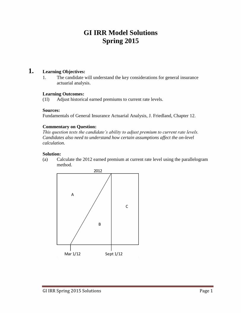
(a) Calculate the 2012 earned premium at current rate level using the parallelogram

method.

2012 2013

A

C

B

Mar 1/12 Sept 1/12


1. Continued

Area Rate Level

(A): 1 – 4/12 – 3/12 = 5/12 1.00

(B): 1/2×6/12×12/12 = 1/4 1.04

(C): 4/12 1.04×0.85

Average rate level = 5 1 41.0 1.04 1.04 0.85 0.97133312 4 12

Current rate level = 1.04×0.85×1.05×1.07 = 0.993174

On-level factor = 0.993174 ÷ 0.971333 = 1.022485

2012 on-level earned premium = 475,000×1.022485 = 485,680

(b) Explain why you would expect the 2012 earned premium at current rate level to

be greater or less than the answer from part (a) if all policies were twelve-month

policies instead of six-month policies.

With all policies being 12-month policies, more of the area of 2012 would be at

lower rates (higher percentage at rate level 1.00, lower percentage at rate level

1.04). Therefore, the average rate level in 2012 would be lower. The current rate

level remains unchanged. Therefore, the on-level factor would be higher than the

value from part (a).

(c) Explain how the increase in the state-mandated minimum policy limits would

affect the on-level calculation from part (a).

The average premium would increase to reflect such a change, but claims would

be expected to increase as policyholders would receive more coverage.

Therefore, expect no change to the on-level calculation.


2. Learning Objectives: 2. The candidate will understand how to calculate projected ultimate claims and

claims-related expenses.

3. The candidate will understand financial reporting of claim liabilities and premium

liabilities.

6. The candidate will understand the need for monitoring results.

Learning Outcomes:

(2b) Estimate ultimate claims using various methods: development method, expected

method, Bornhuetter Ferguson method, Cape Cod method, frequency-severity

methods, Berquist-Sherman methods.

(3c) Describe the components of claim liabilities in the context of financial reporting.

(6a) Describe the role of monitoring in ultimate values and pricing.

(6b) Analyze actual claims experience relative to expectations.

Sources:

Fundamentals of General Insurance Actuarial Analysis, J. Friedland, Chapters 16, 17, 23

and 36.


This question tests the candidate’s ability to estimate ultimate claims using the expected

method and the Bornhuetter Ferguson method. Candidates also need to calculate unpaid

claims, split by case estimate and IBNR. This question also requires candidates to

estimate expected paid claims for an interim period between actuarial analyses using the

approach of Friedland Chapter 36, as well as understand reasons why the difference

between actual and expected reported claims can be different than the difference between

actual and expected paid claims.

Solution:

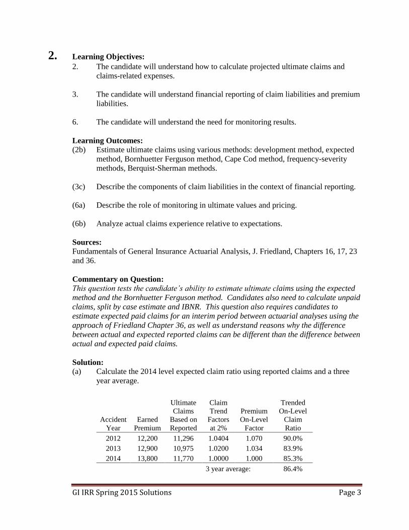
(a) Calculate the 2014 level expected claim ratio using reported claims and a three

year average.

Accident

Year Earned

Premium

Ultimate

Claims

Based on

Reported

Claim

Trend

Factors

at 2%

Premium

On-Level

Factor

Trended

On-Level

Claim

Ratio

2012 12,200 11,296 1.0404 1.070 90.0%

2013 12,900 10,975 1.0200 1.034 83.9%

2014 13,800 11,770 1.0000 1.000 85.3%

3 year average: 86.4%


2. Continued

Trended On-Level Claim Ratio = (Ultimate Claims)(Claim Trend Factor)

(Earned Premium)(On-Level Factor)

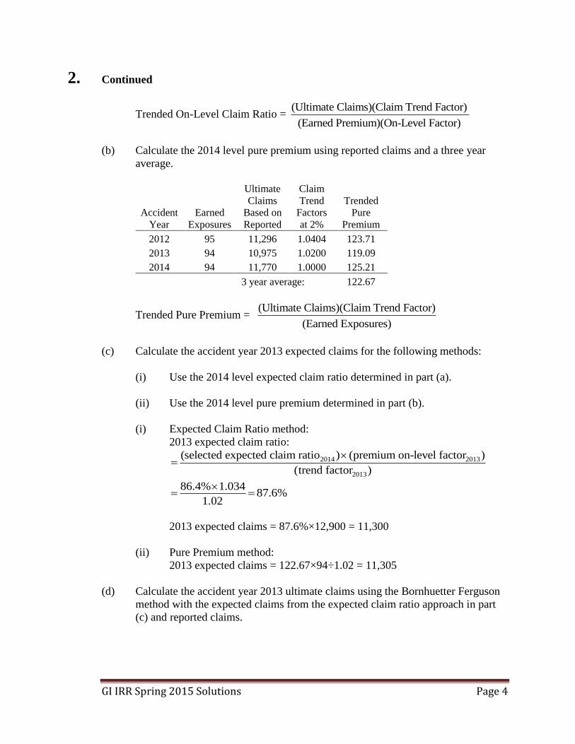
(b) Calculate the 2014 level pure premium using reported claims and a three year

average.

Accident

Year Earned

Exposures

Ultimate

Claims

Based on

Reported

Claim

Trend

Factors

at 2%

Trended

Pure

Premium

2012 95 11,296 1.0404 123.71

2013 94 10,975 1.0200 119.09

2014 94 11,770 1.0000 125.21

3 year average: 122.67

Trended Pure Premium = (Ultimate Claims)(Claim Trend Factor)

(Earned Exposures)

(c) Calculate the accident year 2013 expected claims for the following methods:

(i) Use the 2014 level expected claim ratio determined in part (a).

(ii) Use the 2014 level pure premium determined in part (b).

(i) Expected Claim Ratio method:

2013 expected claim ratio:

2014 2013

2013

(selected expected claim ratio ) (premium on-level factor )

(trend factor )

86.4% 1.03487.6%

1.02

2013 expected claims = 87.6%×12,900 = 11,300

(ii) Pure Premium method:

2013 expected claims = 122.67×94÷1.02 = 11,305

(d) Calculate the accident year 2013 ultimate claims using the Bornhuetter Ferguson

method with the expected claims from the expected claim ratio approach in part

(c) and reported claims.


2. Continued

Implicit development factor = (10,975/8,970) = 1.224

Expected % undeveloped = 1 – 1/1.224 = 18.3%

Expected claims from part (c): 11,300

Expected claims undeveloped = 18.3% × 11,300 = 2,068

Reported claims @ Dec. 31, 2013: 8,970

Estimated ultimate claims = 2,068 + 8,970 = 11,038

(e) Calculate the accident year 2013 unpaid claims using the ultimate claims

calculated in part (d). Show the case estimate and indicated IBNR separately.

Unpaid = ultimate claims from part (d) – paid to date = 11,038 – 6,950 = 4,088

IBNR = ultimate claims – reported to date = 11,038 – 8,970 = 2,068

Case = Unpaid – IBNR = 2,020

(f) Calculate the difference between the actual and expected paid claims from

December 31, 2014 through March 31, 2015 for accident year 2014, using linear

interpolation of the expected percent paid derived from the implied paid

cumulative development factors.

Commentary on Question: Candidates need to use the formula in the textbook, as the expected paid at March

31, 2015 is not equal to the ultimate claims multiplied by the expected percent

paid at March 31, 2015.

Expected % paid at December 31, 2014 for accident year 2013 = (Cumulative

Paid) / (Selected Ultimate Based on Paid) = 6,950 / 10.544 = 65.9%

Expected % paid at December 31, 2014 for accident year 2014 = 4,100 /

11,196 = 36.6%

Interpolate to estimate accident year 2014 percent paid at March 31, 2015 =

= 36.6%×0.75 + 65.9%×0.25 = 43.9%

Actual claims paid between December 31, 2014 and March 31, 2015 = 4,790

– 4,100 = 690

Expected paid between December 31, 2014 and March 31, 2015 =

11,196 4,100(43.9% 36.6%) 817

1 36.6%

Difference between actual and expected paid claims between December 31,

2014 and March 31, 2015 = 690 – 817 = –127

(g) State two possible reasons why the difference between the actual and expected

reported claims is different than the difference between the actual and expected

paid claims for accident year 2014.


2. Continued

Possible reasons include:

The payment pattern may be changing.

There may be an issue with claim payments in the first quarter (e.g.,

processing delay).


3. Learning Objectives: 4. The candidate will understand trending procedures as applied to ultimate claims,

exposures and premiums.

5. The candidate will understand how to apply the fundamental ratemaking

techniques of general insurance.

Learning Outcomes:

(4a) Identify the time periods associated with trending procedures.

(5f) Calculate overall rate change indications under the claims ratio and pure premium

methods.

Sources:

Fundamentals of General Insurance Actuarial Analysis, J. Friedland, Chapters 25 and 31.


This question requires candidates to estimate trended ultimate severity for ratemaking

purposes. Candidates also need to understand the adjustments that may be required to

complements of credibility.

Solution:

(a) Explain two situations where the pure premium ratemaking approach is preferred

to the claim ratio ratemaking approach.

Any two of the following are acceptable:

When trended earned premiums are not available or not reliable

For self-insured entities

With new products/new lines of business (i.e., where historical claim ratios

are unavailable)

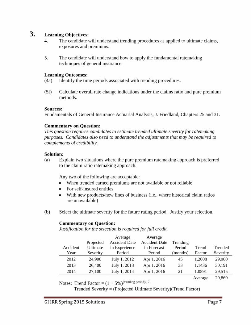
(b) Select the ultimate severity for the future rating period. Justify your selection.

Commentary on Question: Justification for the selection is required for full credit.

Accident

Year

Projected

Ultimate

Severity

Average

Accident Date

in Experience

Period

Average

Accident Date

in Forecast

Period

Trending

Period

(months)

Trend

Factor

Trended

Severity

2012 24,900 July 1, 2012 Apr 1, 2016 45 1.2008 29,900

2013 26,400 July 1, 2013 Apr 1, 2016 33 1.1436 30,191

2014 27,100 July 1, 2014 Apr 1, 2016 21 1.0891 29,515

Average 29,869

Notes: Trend Factor = (1 + 5%)(trending period)/12

Trended Severity = (Projected Ultimate Severity)(Trend Factor)


3. Continued

Selected Trended Severity is 29,869. This selection is reasonable as there is no

evidence of any outliers.

(c) Describe an adjustment, if any, that may be required for each of these possible

complements of credibility.

The pure premium underlying the current rates needs to be adjusted to the cost

level of the forecast period.

The pure premium based on industry experience needs to be adjusted to reflect the

insurer’s mix of exposures and the cost level of the forecast period.


4. Learning Objectives: 3. The candidate will understand financial reporting of claim liabilities and premium

liabilities.

Learning Outcomes:

(3b) Estimate unpaid unallocated loss adjustment expenses using ratio and count-based

methods.

Sources:



This question tests the Wendy Johnson count-based method to calculate unallocated loss

adjustment expenses.

Solution:

(a) Explain two weaknesses of the classical paid-to-paid unallocated loss adjustment

expenses (ULAE) estimation method.


When there are significant changes in exposure volume occurring

Inflationary periods

Business in a run-off state

ULAE associated with IBNYR is very different from IBNR

(b) Estimate unpaid ULAE as of December 31, 2014 using a simple three-year

average of historical experience.

Calendar

Year

Paid

ULAE

(000)

Counts Average

ULAE per

Weighted

Count

Newly

Reported Open Closed

Weighted

Total

(1) (2) (3) (4) (5) (6) (7)

2012 1,862 1,550 577 1,580 872 2,135

2013 2,100 1,700 614 1,663 936 2,244

2014 1,995 1,685 621 1,678 940 2,122

Selected Average ULAE per Weighted Count 2,167

Notes: (6) = [0.2×(3)] + [0.7×(4)] + [0.1×(5)]

(7) = 1000×(2) / (6)


4. Continued

Calendar

Year

Counts

Trending

Period in

Years

Prospective

Trend

Trended

Average

ULAE

Estimated

Unpaid

ULAE (000)

Newly

Reported

During

the Year

Open at

End of

Year

Closed

During

the

Year

Weighted

Total

(1) (2) (3) (4) (5) (6) (7) (8) (9)

2015 665 316 970 451 1 1.030 2,232 1,007

2016 150 82 384 126 2 1.061 2,299 290

2017 - - 82 8 3 1.093 2,368 19

1,315

Notes: (5) = [0.2×(2)] + [0.7×(3)] + [0.1×(4)]

(8) = 2,167×(7)

(9) = (5)(8) / 1,000


5. Learning Objectives: 5. The candidate will understand how to apply the fundamental ratemaking


Learning Outcomes:

(5j) Perform individual risk rating using standard plans.

Sources:

“The Mathematics of Excess of Loss Coverages and Retrospective Rating – A Graphical

Approach,” Lee, Y., Casualty Actuarial Society, 1988 Proceedings, Vol. LXXV


This question tests the understanding of retrospective rating.

Solution:

(a) Explain what the Table L savings and Table L charge indicate.

The Table L savings at entry ratio r is the expected amount by which the risk’s

actual limited loss falls short of r times the expected unlimited loss, divided by

the expected unlimited loss.

The Table L charge at entry ratio r is the expected amount by which the risk’s

actual limited loss exceeds r times the expected unlimited loss, divided by the

expected unlimited loss, PLUS the loss elimination ratio associated with the per

accident limitation.

(b) Draw a graph with cumulative claim frequency along the x-axis and entry ratio

along the y-axis, and identify the areas on the graph corresponding to r* and

* r .


5. Continued

r* = (A + B)

* r = (B + D + E)

(c) Demonstrate the validity of the fundamental relation above using the areas of the

graph.

* r k E

* * (the lower rectangle) 1 (the area under the lower curve)r r k r k

= E + A + B + C – (C + E) = A + B

(d) Define r* for the limiting case where losses are all equal.

krr 1 ,0* and krkrr 1 ,1*




Learning Outcomes:




Sources:



This question tests the application of the development method, including the

understanding of Boor’s algebraic method. Candidates also need to understand the

incorporation of benchmark data when selecting tail factors.

Solution:

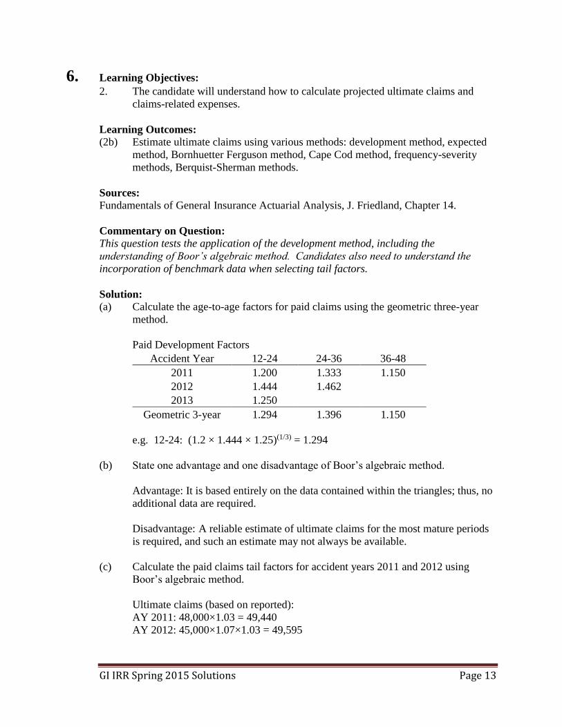
(a) Calculate the age-to-age factors for paid claims using the geometric three-year

method.

Paid Development Factors

Accident Year 12-24 24-36 36-48

2011 1.200 1.333 1.150

2012 1.444 1.462

2013 1.250

Geometric 3-year 1.294 1.396 1.150

e.g. 12-24: (1.2 × 1.444 × 1.25)(1/3) = 1.294

(b) State one advantage and one disadvantage of Boor’s algebraic method.

Advantage: It is based entirely on the data contained within the triangles; thus, no

additional data are required.

Disadvantage: A reliable estimate of ultimate claims for the most mature periods

is required, and such an estimate may not always be available.

(c) Calculate the paid claims tail factors for accident years 2011 and 2012 using

Boor’s algebraic method.

Ultimate claims (based on reported):

AY 2011: 48,000×1.03 = 49,440

AY 2012: 45,000×1.07×1.03 = 49,595


6. Continued

Paid claims at 48 months:

AY 2011: 46,000

AY 2012: 38,000×1.15 = 43,700

Tail factors:

AY 2011: 49,440 ÷ 46,000 = 1.075

AY 2012: 49,595 ÷ 43,700 = 1.135

(d) State two common sources of benchmark data.


Industry experience:

o In the U.S. this includes A.M. Best, ISO, NCCI, and RAA

o In Canada this includes Insurance Bureau of Canada and General

Insurance Statistical Agency

Data from affiliate companies

Experience from similar lines of business

(e) State two potential limitations of benchmark data.


Differences in the way claims are adjusted or reserved

Differences in the potential for long-developing high value claims

Differences in the initial reporting pattern for claims

Differences in the adjudication process for litigated claims

Statistical reliability of the benchmark triangle

(f) Explain how you would evaluate and incorporate the benchmark data in your tail

factor selection.

Compare the age-to-age factors of benchmark data against the insurer’s data for

earlier ages of development. If patterns are similar then consider using; if not

then adjust or reject.




Learning Outcomes:

(5h) Calculate deductible factors, increased limits factors, and coinsurance penalties.

Sources:



This question tests the understanding of and application of deductibles. In addition, the

question tests understanding of coinsurance.

Solution:

(a) Explain the importance of consistency in setting deductible factors.

Any of the following descriptions are acceptable:

Important because it tests the reasonableness of the factors.

The marginal premium per 1,000 of coverage should decrease as the

deductible increases.

Insured would not expect to pay marginally more for each additional 1,000 of

coverage, because the probability of claims at each successively increasing

layer is less than that of the immediately preceding layer.

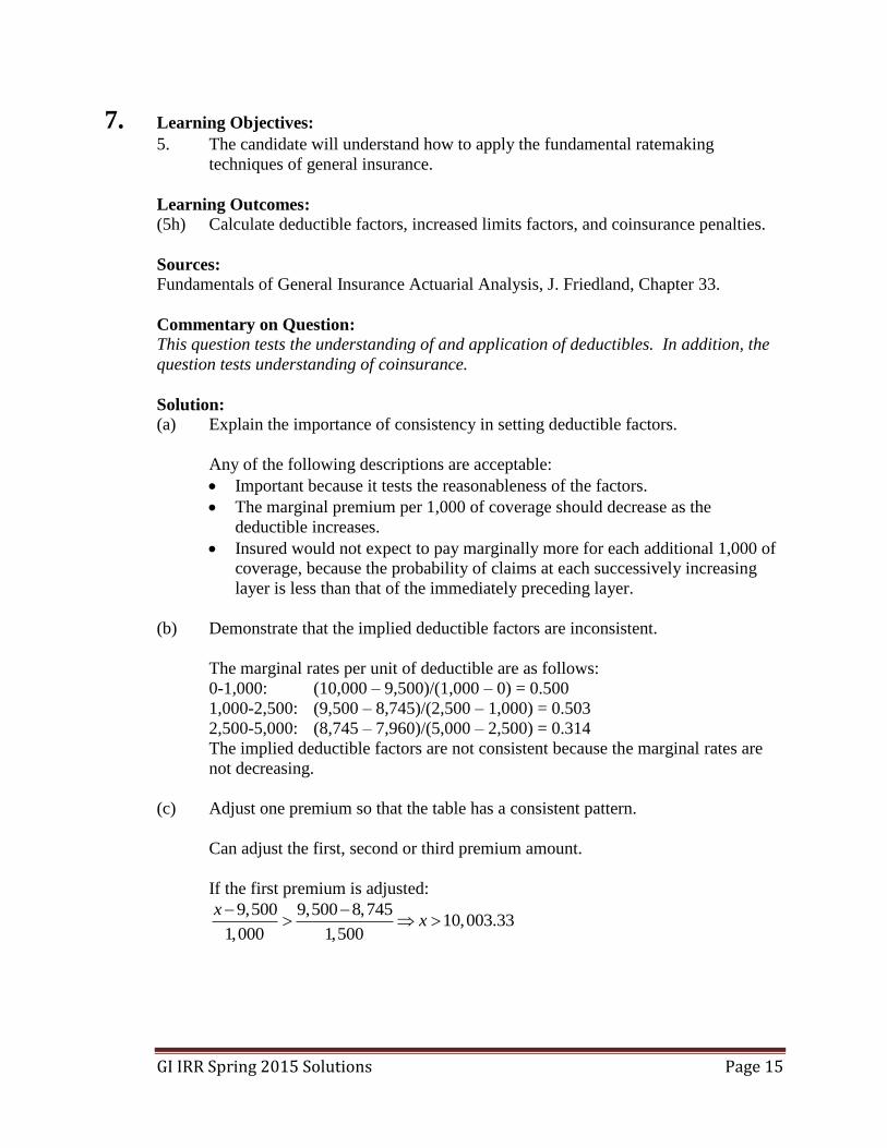
(b) Demonstrate that the implied deductible factors are inconsistent.

The marginal rates per unit of deductible are as follows:

0-1,000: (10,000 – 9,500)/(1,000 – 0) = 0.500

1,000-2,500: (9,500 – 8,745)/(2,500 – 1,000) = 0.503

2,500-5,000: (8,745 – 7,960)/(5,000 – 2,500) = 0.314

The implied deductible factors are not consistent because the marginal rates are

not decreasing.

(c) Adjust one premium so that the table has a consistent pattern.

Can adjust the first, second or third premium amount.

If the first premium is adjusted:

9,500 9,500 8,74510,003.33

1,000 1,500

xx


7. Continued

If the second premium is adjusted:

premium (x) must meet two conditions:

1. 10,000 8,745

9,4981,000 1,500

x xx

2. 8,745 8,745 7,960

9,2161,500 2,500

xx

Result: 9,216 < x < 9,498

If the third premium is adjusted:

premium (x) must meet two conditions:

1. 9,500 7,960

8,922.501,500 2,500

x xx

2. 9,500 10,000 9,500

8,7501,500 1,000

xx

Result: 8,750 < x < 8,922.50

(d) Define the following terms:

(i) Franchise deductible

(ii) Time deductible

(i) Franchise deductible of 1,000: losses below 1,000 are not covered whereas

a loss greater than 1,000 is covered in full. For example, a loss of 500

would not be covered but a loss of 1,100 would be covered in full.

(ii) Time deductible: a time delay between the occurrence of the covered

incident and the start of the insurance coverage.

(e) Explain how the responsibility for claims handling differs between large

deductible policies and self-insured retention policies.

Large deductible policies: the insurer is typically involved in the adjustment and

payment of all claims for insureds with deductibles.

Self-insured retention (SIR): insureds with an SIR are responsible for the

adjustment and payment of all claims that fall within the SIR.


7. Continued

(f) Illustrate graphically what the insurer would pay for losses from zero up to the

property value in the following situations:

(i) 100% coinsurance requirement applicable to the loss before the deductible

(ii) No coinsurance requirement

0

20,000

40,000

60,000

80,000

100,000

120,000

140,000

160,000

0

10

00

0

20

00

0

30

00

0

40

00

0

50

00

0

60

00

0

70

00

0

80

00

0

90

00

0

10

00

00

11

00

00

12

00

00

13

00

00

14

00

00

15

00

00

16

00

00

17

00

00

18

00

00

19

00

00

20

00

00

Insu

rer

Pay

s

Loss

Amount Insurer Pays

With Coinsurance No Coinsurance




Learning Outcomes:

(2a) Use loss development triangles for investigative testing.




Sources:



This question tests the candidate’s ability to diagnose the triangle of average case

estimates, as well as the understanding of the Berquist-Sherman adjustments when there

has been a change in case reserve adequacy.

Solution:

(a) Explain two reasons why an actuary must be careful in using this investigative

tool to reach a conclusion on the level of overall adequacy of case estimates.

1. What might appear to be changes in the average case estimates may simply be

due to the presence or absence of large claims.

2. Any changes that affect counts, reported or closed, would influence the

denominator of this average value.

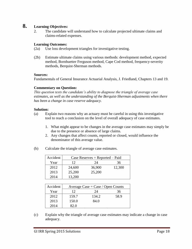
(b) Calculate the triangle of average case estimates.

Accident Case Reserves = Reported – Paid

Year 12 24 36

2012 24,600 36,900 12,300

2013 25,200 25,200

2014 13,200

Accident Average Case = Case / Open Counts

Year 12 24 36

2012 159.7 134.2 58.9

2013 150.0 84.0

2014 82.0

(c) Explain why the triangle of average case estimates may indicate a change in case

adequacy.


8. Continued

Changes down each column (accident year to accident year) should be explained

by the trend rate only, so if it is different than trend, possible changes in case

reserve adequacy are indicated.

(d) Adjust the reported claims triangle using the Berquist-Sherman methodology.

Adjusted Average Case Reserves = Average Case (latest diagonal), divided by

trend

Accident Adjusted Average Case Reserves

Year 12 24 36

2012 77.3 81.6 58.9

2013 79.6 84.0

2014 82.0

e.g. 82.0 / 1.03 = 79.6 Adjusted Case Reserves = (Adjusted Average Case)(Open Counts)

Accident Adjusted Case Reserves

Year 12 24 36

2012 11,901 22,427 12,300

2013 13,373 25,200

2014 13,200 Adjusted Reported Claims = (Adjusted Case Reserves) + (Paid Claims)

Accident Adjusted Reported Claims

Year 12 24 36

2012 61,101 83,927 104,600

2013 63,773 88,200

2014 66,000

(e) Describe what adjustments may be appropriate to the tail factor.

If case reserve adequacy is falling, the possibility of an increased tail factor exists.

But if the line of business is short-tailed, it may be fully developed after three

years. Consider other available information.

(f) Explain why the IBNR based on the adjusted reported claims is likely to be higher

or lower than the IBNR based on the unadjusted reported claims.

Unadjusted claims are likely to understate the ultimate claims estimate (higher

reported claims will result in lower development factors and therefore lower

IBNR). The Berquist-Sherman adjustment will produce a higher ultimate claims

estimate, and therefore higher IBNR.


9. Learning Objectives: 7. The candidate will understand the nature and application of catastrophe models

used to manage risks from natural disasters.

Learning Outcomes:

(7b) Apply catastrophe models to insurance ratemaking, portfolio management, and

risk financing.

Sources:

Catastrophe Modeling: A New Approach to Managing Risk, Grossi, P. and Kunreuther,

H., Chapter 7.


This questions tests the candidate’s understanding of various risk financing strategies for

catastrophe models.

Solution:

(a) Indicate for each of strategies 1 and 2 if it meets or does not meet XYZ

management’s requirement. Justify your conclusions.

Commentary on Question: Candidates need to specifically say whether the strategy meets or does not meet

management’s requirement to get full credit.

For strategy 1, the 1% probability is at 0.7(700) = 490 and thus the requirement is

met.

For strategy 2, the 1% probability is at 400 + 0.2(700 – 400) = 460 and thus the

requirement is met.

(b) State the advantages and disadvantages of selecting strategy 1 instead of strategy

2.

The advantage of strategy 1 is that coverage is retained and so a proportion of

expected profits is not passed to the reinsurer.

The disadvantage is that 30% of expected profits are surrendered. This is likely

more than will be given up if reinsurance is purchased.

(c) Explain why, based on the information above, it is not possible to determine

whether strategy 3 meets or does not meet XYZ management’s requirement.

For strategy 3, it might meet the requirement, but without an exceedance curve for

the industry portfolio and an evaluation of basis risk, that cannot be known for

sure.


9. Continued

(d) Compare, with explanations, strategies 2 and 3 with regard to moral hazard and

basis risk.

Strategy 2:

No basis risk as losses from catastrophe are paid on the basis of actual

company losses.

This strategy has moral hazard, but mechanisms to reduce moral hazard can

be built in to indemnity-based transactions.

Strategy 3:

Index-based transactions reduce moral hazard, since an individual cedant has

little control over industry losses.

Cedant is exposed to basis risk to the extent that its own exposures - and

therefore losses - differ in kind and geographical distribution from that of the

industry's, or from that of the index used to determine the payoff of the

contract.




Learning Outcomes:

(5j) Perform individual risk rating using standard plans.

Sources:



This question tests the understanding of experience rating and schedule rating.

Solution:

(a) Explain why insurers use experience rating.

Insurers use experience rating so that their premium reflects, at least in part, the

insured’s own claim experience.

(b) Explain why you may choose to base credibility on premium in individual risk

rating.

Credibility is usually based on exposures or premium in individual risk rating so

that a larger insurer receives greater credibility for its actual loss experience.

(c) Explain why insurers use schedule rating.

Insurers use schedule rating to incorporate judgment about specific risk

characteristics of the insured that are either not considered at all or are not

adequately reflected in the manual rating process (e.g., in the manual rates, rating

rules, rating factors, and rating algorithm).

(d) State three examples of risk characteristics used in schedule rating plans.

Any three of the following are acceptable:

Features of workplace maintenance or operation, including the condition and

upkeep of the premises and equipment

Availability of medical facilities in or near the workplace

Quality of police and fire protection

Safety equipment/devices present in/missing from the workplace

Qualification of employees including employee training, selection, and

supervision

Construction features and maintenance

Accommodations/cooperation with insurer by management

Considerations related to policy expenses


10. Continued

(e) Define premium discounts and expense constants.

Premium discount plans are used primarily with U.S. workers compensation to

recognize the administrative cost savings associated with insureds with larger

premiums.

An expense constant or an acquisition expense load may be used to cover an

insurer’s cost of policy issuance, auditing, and management.

(f) Select two items from the list above and explain how actuaries can assist in their

development and maintenance.


Trend factors: use similar methods to those for manual rating, conducted at

limits that are consistent with any large claim capping that is used for the

experience rating plan

Development factors: use similar methods to those for manual rating; select

development factors based on analysis of reported claims summarized in

development triangles

Expected claim ratios: use similar methods to those for manual rating

Large claim thresholds: use similar methods to those for manual rating

Credibility: actuary can determine credibility values

(g) Explain two problems with a retrospective rating plan in this case.


The insureds in the plan are small and may have variable claims experience.

Particularly for small insureds, fire, windstorm and earthquake exposures can

be catastrophe prone.

The lure of a large increase in premium may seem to overshadow the risk, but

the future could hold large individual fires or catastrophes that may be in

excess of plan maxima.

The experience, even for the entire group, may not be very predictable.




4. The candidate will understand trending procedures as applied to ultimate claims,


Learning Outcomes:




(4b) Describe the influences on frequency and severity of changes in deductibles,

changes in policy limits, and changes in mix of business.

Sources:


Solution:

(a) State two other changes in historical data that would require adjustment.

Commentary on Question: Changes in limits, deductibles, inflation, etc., are the kinds of items that trend is

measuring, so they are not adjustments that must be made prior to analyzing

trend.


Catastrophe claims

Seasonality

Changes resulting from tort and product reform

Legislated benefit-level changes

Changes in claim settlement

(b) State three information sources you may take into account.


Professional judgment

Insurer’s own experience

Trend rates indicated based on analyses of industry data

Trends in the general economy

The trend rate selected for pricing purposes

The trend rate selected in the prior analysis of ultimate claims

The trend rates selected by competitors if such information is available


11. Continued

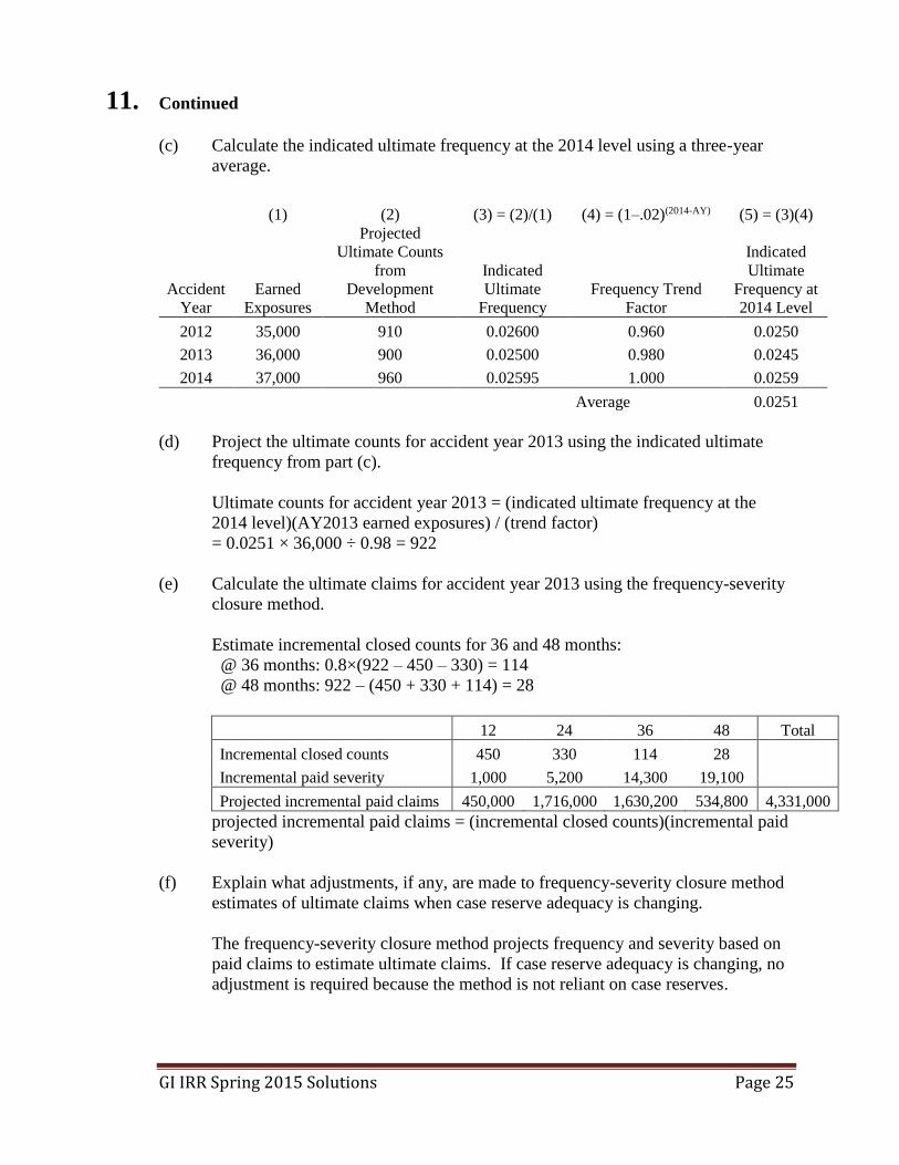
(c) Calculate the indicated ultimate frequency at the 2014 level using a three-year

average.

(1) (2) (3) = (2)/(1) (4) = (1–.02)(2014-AY) (5) = (3)(4)

Accident

Year

Earned

Exposures

Projected

Ultimate Counts

from

Development

Method

Indicated

Ultimate

Frequency

Frequency Trend

Factor

Indicated

Ultimate

Frequency at

2014 Level

2012 35,000 910 0.02600 0.960 0.0250

2013 36,000 900 0.02500 0.980 0.0245

2014 37,000 960 0.02595 1.000 0.0259

Average 0.0251

(d) Project the ultimate counts for accident year 2013 using the indicated ultimate

frequency from part (c).

Ultimate counts for accident year 2013 = (indicated ultimate frequency at the

2014 level)(AY2013 earned exposures) / (trend factor)

= 0.0251 × 36,000 ÷ 0.98 = 922

(e) Calculate the ultimate claims for accident year 2013 using the frequency-severity

closure method.

Estimate incremental closed counts for 36 and 48 months:

@ 36 months: 0.8×(922 – 450 – 330) = 114

@ 48 months: 922 – (450 + 330 + 114) = 28

12 24 36 48 Total

Incremental closed counts 450 330 114 28

Incremental paid severity 1,000 5,200 14,300 19,100

Projected incremental paid claims 450,000 1,716,000 1,630,200 534,800 4,331,000

projected incremental paid claims = (incremental closed counts)(incremental paid

severity)

(f) Explain what adjustments, if any, are made to frequency-severity closure method

estimates of ultimate claims when case reserve adequacy is changing.

The frequency-severity closure method projects frequency and severity based on

paid claims to estimate ultimate claims. If case reserve adequacy is changing, no

adjustment is required because the method is not reliant on case reserves.


12. Learning Objectives: 4. The candidate will understand trending procedures as applied to ultimate claims,


5. The candidate will understand how to apply the fundamental ratemaking


Learning Outcomes:

(4a) Identify the time periods associated with trending procedures.

(5b) Calculate expenses used in ratemaking analyses including expense trending

procedures.

Sources:



This question tests the expense provisions that are used in ratemaking.

Solution:

(a) Select the variable expense percentage to use for ratemaking based on the

historical ratio of variable expense to premium. Justify your selection.

Commentary on Question: Justification is required for full credit.

(1) (2) (3) (4) = (3)×0.4 (5) = (4)/(1)

Calendar

Year

Earned

Premium

Earned

Exposures

Total

General

Expenses Variable % Variable

2012 4,019,000 2,770 452,100 180,840 4.50%

2013 4,307,000 2,910 495,300 198,120 4.60%

2014 4,571,000 2,930 502,800 201,120 4.40%

Total: 12,897,000 8,610 1,450,200 580,080 4.50%

Selection: 4.5%

Justification: No indication of outlier or trend, so the total is a reasonable

selection.

(b) Select the fixed expense per exposure to use for ratemaking. Justify your

selection.


12. Continued

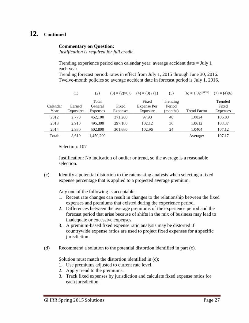
Commentary on Question: Justification is required for full credit.

Trending experience period each calendar year: average accident date = July 1

each year.

Trending forecast period: rates in effect from July 1, 2015 through June 30, 2016.

Twelve-month policies so average accident date in forecast period is July 1, 2016.

(1) (2) (3) = (2)×0.6 (4) = (3) / (1) (5) (6) = 1.02[(5)/12] (7) = (4)(6)

Calendar

Year

Earned

Exposures

Total

General

Expenses

Fixed

Expenses

Fixed

Expense Per

Exposure

Trending

Period

(months) Trend Factor

Trended

Fixed

Expenses

2012 2,770 452,100 271,260 97.93 48 1.0824 106.00

2013 2,910 495,300 297,180 102.12 36 1.0612 108.37

2014 2,930 502,800 301,680 102.96 24 1.0404 107.12

Total: 8,610 1,450,200 Average: 107.17

Selection: 107

Justification: No indication of outlier or trend, so the average is a reasonable

selection.

(c) Identify a potential distortion to the ratemaking analysis when selecting a fixed

expense percentage that is applied to a projected average premium.

Any one of the following is acceptable:

1. Recent rate changes can result in changes to the relationship between the fixed

expenses and premiums that existed during the experience period.

2. Differences between the average premiums of the experience period and the

forecast period that arise because of shifts in the mix of business may lead to

inadequate or excessive expenses.

3. A premium-based fixed expense ratio analysis may be distorted if

countrywide expense ratios are used to project fixed expenses for a specific

jurisdiction.

(d) Recommend a solution to the potential distortion identified in part (c).

Solution must match the distortion identified in (c):

1. Use premiums adjusted to current rate level.

2. Apply trend to the premiums.

3. Track fixed expenses by jurisdiction and calculate fixed expense ratios for

each jurisdiction.


13. Learning Objectives: 1. The candidate will understand the key considerations for general insurance

actuarial analysis.

Learning Outcomes:

(1k) Estimate written, earned and unearned premiums.

(1l) Adjust historical earned premiums to current rate levels.

Sources:



This question tests the candidate’s understanding of certain details of individual

insurance policies and the ability to make correct calculations of written premium,

earned premium, and unearned premium for various policies. The candidate also needs

to understand earned premiums adjusted to current rate level.

Solution:

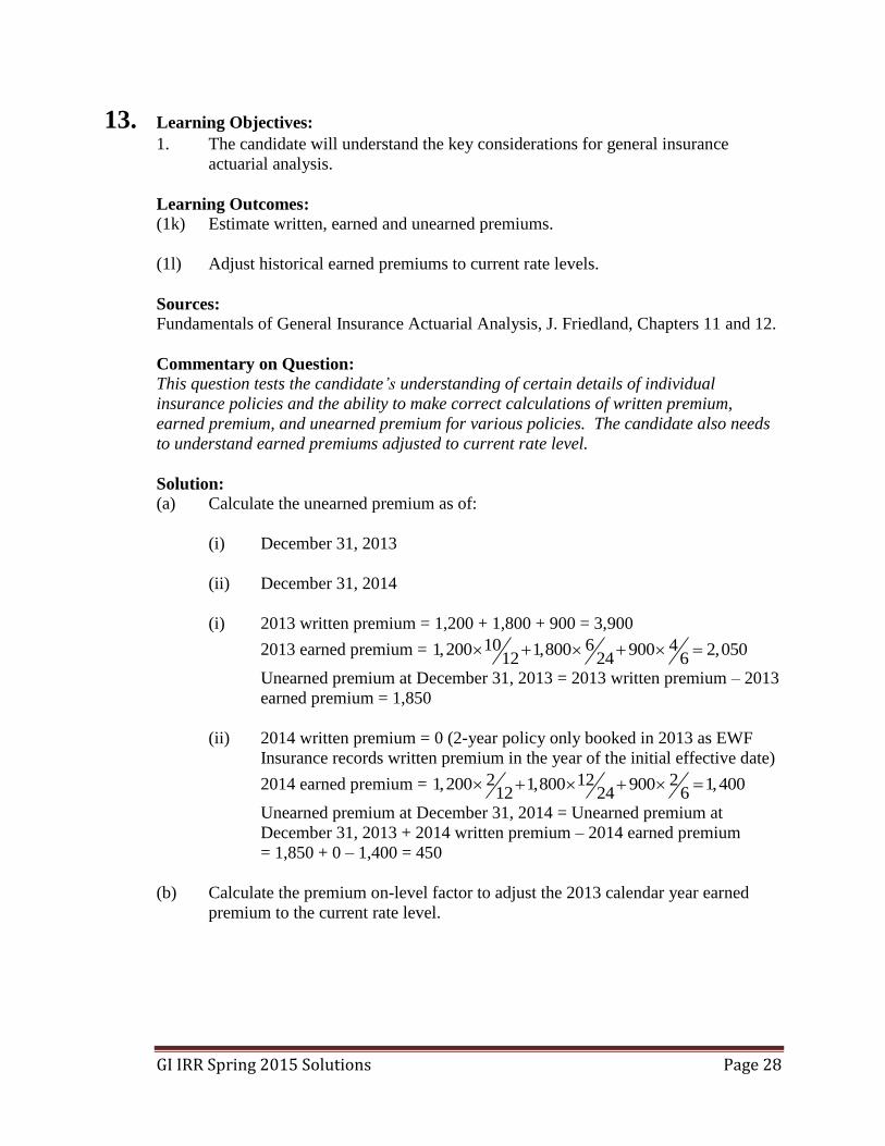
(a) Calculate the unearned premium as of:

(i) December 31, 2013

(ii) December 31, 2014

(i) 2013 written premium = 1,200 + 1,800 + 900 = 3,900

2013 earned premium = 10 6 41,200 1,800 900 2,05012 24 6

Unearned premium at December 31, 2013 = 2013 written premium – 2013

earned premium = 1,850

(ii) 2014 written premium = 0 (2-year policy only booked in 2013 as EWF

Insurance records written premium in the year of the initial effective date)

2014 earned premium = 2 12 21,200 1,800 900 1,40012 24 6

Unearned premium at December 31, 2014 = Unearned premium at

December 31, 2013 + 2014 written premium – 2014 earned premium

= 1,850 + 0 – 1,400 = 450

(b) Calculate the premium on-level factor to adjust the 2013 calendar year earned

premium to the current rate level.


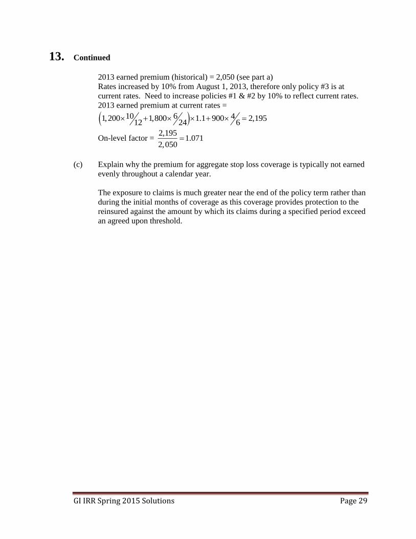
13. Continued

2013 earned premium (historical) = 2,050 (see part a)

Rates increased by 10% from August 1, 2013, therefore only policy #3 is at

current rates. Need to increase policies #1 & #2 by 10% to reflect current rates.

2013 earned premium at current rates =

10 6 41,200 1,800 1.1 900 2,19512 24 6

On-level factor = 2,195

1.0712,050

(c) Explain why the premium for aggregate stop loss coverage is typically not earned

evenly throughout a calendar year.

The exposure to claims is much greater near the end of the policy term rather than

during the initial months of coverage as this coverage provides protection to the

reinsured against the amount by which its claims during a specified period exceed

an agreed upon threshold.




Learning Outcomes:




Sources:



This question tests the understanding of the assumptions and inputs to the Bornhuetter

Ferguson, Benktander, and Cape Cod methods. In addition, candidates needs to estimate

ultimate claims using the Cape Cod and the Generalized Cape Cod method.

Solution:

(a) State the key assumption from the expected method that is used when applying

the Bornhuetter Ferguson method.

Actuaries can better project ultimate values based on an a priori estimate than

from the experience observed to date.

(b) Explain the difference between the inputs to the Bornhuetter Ferguson method

and the inputs to the Benktander method.

Bornhuetter Ferguson method: An input to the Bornhuetter Ferguson method is

the expected claims from the expected method.

Benktander method: The projected ultimate values derived from the Bornhuetter

Ferguson method become the expected value input to the Benktander method.

(c) Compare the expected claims that are used for the Bornhuetter Ferguson method

with the expected claims that are used for the Cape Cod method.

Bornhuetter Ferguson method: Future claim activity is derived from the a priori

estimate of the expected method.

Cape Cod method: Observed claims, adjusted for trend, tort reform and other

measurable changes over time, and observed exposures (adjusted for measurable

changes over time such as rate changes and trend) are used to estimate the cost

per exposure which is used to calculate the expected values.


14. Continued

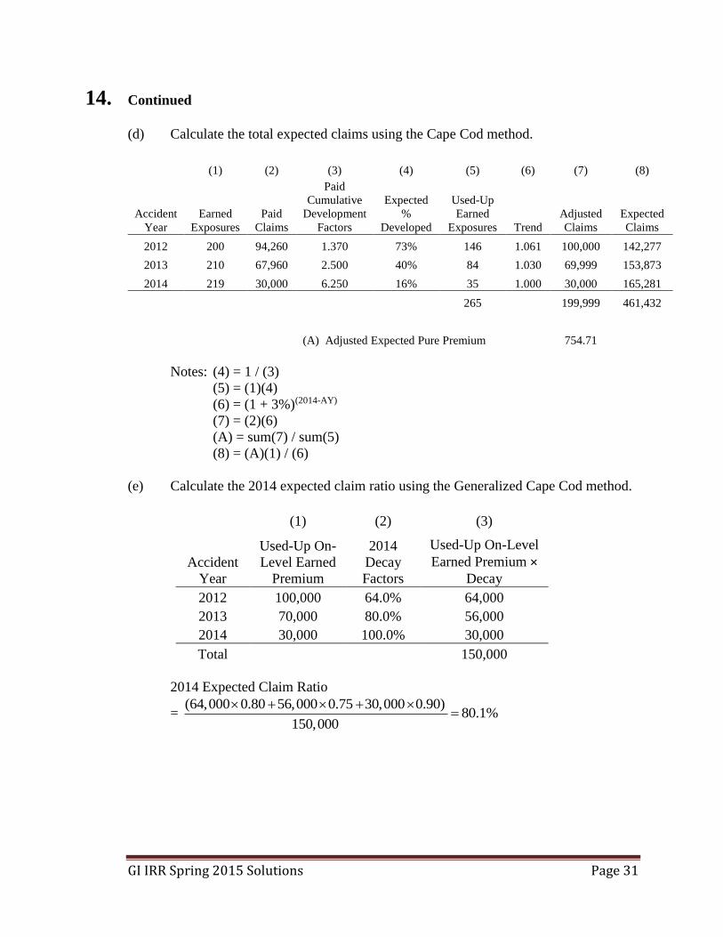
(d) Calculate the total expected claims using the Cape Cod method.

(1) (2) (3) (4) (5) (6) (7) (8)

Accident

Year

Earned

Exposures

Paid

Claims

Paid

Cumulative

Development

Factors

Expected

%

Developed

Used-Up

Earned

Exposures Trend

Adjusted

Claims

Expected

Claims

2012 200 94,260 1.370 73% 146 1.061 100,000 142,277

2013 210 67,960 2.500 40% 84 1.030 69,999 153,873

2014 219 30,000 6.250 16% 35 1.000 30,000 165,281

265 199,999 461,432

(A) Adjusted Expected Pure Premium 754.71

Notes: (4) = 1 / (3)

(5) = (1)(4)

(6) = (1 + 3%)(2014-AY)

(7) = (2)(6)

(A) = sum(7) / sum(5)

(8) = (A)(1) / (6)

(e) Calculate the 2014 expected claim ratio using the Generalized Cape Cod method.

(1) (2) (3)

Accident

Year

Used-Up On-

Level Earned

Premium

2014

Decay

Factors

Used-Up On-Level

Earned Premium ×

Decay

2012 100,000 64.0% 64,000

2013 70,000 80.0% 56,000

2014 30,000 100.0% 30,000

Total 150,000

2014 Expected Claim Ratio

= (64,000 0.80 56,000 0.75 30,000 0.90)

80.1%150,000




Learning Outcomes:

(2d) Explain the effect of changing conditions on the projection methods cited in (b).

Sources:



This question tests the understanding of how various changing conditions affect the

estimates of ultimate claims.

Solution:

(a) Explain how the expected claims in each of the Bornhuetter Ferguson and Cape

Cod methods responds to deterioration in claims experience.

In the Bornhuetter Ferguson method, the expected claims are based on an a priori

estimate and do not change unless the actuary deliberately makes a change.

In the Cape Cod method, the expected claims are a function of the reported claims

to date.

(b) Explain whether the Bornhuetter Ferguson method or Cape Cod method is more

responsive to a deterioration in claims experience.

For the Cape Cod method, deterioration in the claims experience will be reflected

to some extent in the expected claims. Thus, the Cape Cod method is more

responsive to a change in claims experience.

(c) Explain which projection method is likely to produce the most accurate estimate

of ultimate claims if there is an unforeseen and unquantified increase in case

reserve adequacy in recent years.

The expected method is likely to produce the most accurate estimate of ultimate

claims if there is an unforeseen and unquantified increase in case reserve

adequacy in recent years. All other methods incorporate actual reported claims

experience which will reflect a distortion caused by the change in case reserve

adequacy.

(d) Explain whether a change in policy exclusions is more likely to cause patterns to

change on an accident or a calendar year basis.


15. Continued

Accident year basis: Changes in policy exclusions occur on a prospective policy

year basis, rather than affecting all historical open claims. Therefore, accident

year claims experience best reflects policy year changes.

(e) Explain whether a change in loss trend is more likely to cause patterns to change

on an accident or a calendar year basis.

Calendar year basis: Trend changes are usually driven by external conditions

which typically affect all open claims. Therefore, trend changes are most likely to

affect an entire diagonal of open claims, regardless of accident year.


16. Learning Objectives: 7. The candidate will understand the nature and application of catastrophe models

used to manage risks from natural disasters.

Learning Outcomes:

(7a) Describe the structure of catastrophe models.

(7b) Apply catastrophe models to insurance ratemaking, portfolio management, and

risk financing.

Sources:

Catastrophe Modeling: A New Approach to Managing Risk, Grossi, P. and Kunreuther,

H., Chapters 3 and 5.


This question tests the factors that are used in the various catastrophe modules.

Solution:

(a) Indicate, for each of the four factors listed by the CEA, which module or modules

use that particular factor. Support your selections.

Commentary on Question: Support for the selections is required for full credit.

1. Location: Hazard and Inventory

2. Soil: Hazard

3. Construction: Inventory and Vulnerability and Loss

4. Age: Inventory and Vulnerability and Loss

Explanations:

Hazard module identifies the location of faults and the risk associated with

each (with soil part of that)

Inventory module contains location, construction, and age (among others), but

not soil type

Vulnerability module measures building damage given the event and is related

to construction and age

Loss module translates the event into money which depends on construction

and age

(b) Propose two additional factors that might be considered. Support your proposal.


Presence of retrofitting (was actually called out in the other parts of the rules)

Building occupancy

Building codes at time of construction


17. Learning Objectives: 3. The candidate will understand financial reporting of claim liabilities and premium

liabilities.

Learning Outcomes:

(3f) Evaluate premium liabilities.

Sources:



This question tests the determination of premium liabilities.

Solution:

(a) Calculate net unearned premium as of December 31, 2014.

Net unearned premium = (Net written premium × Development factor) – Net

earned premium = 1,000,000×1.04 – 500,000 = 540,000

(b) Calculate net premium liabilities as of December 31, 2014.

Expected Net Claims = Net unearned premium × 80% 432,000

Expected Net ULAE = Expected Net Claims × 15% 64,800

Expected Net Claims and ULAE 496,800

Selected Maintenance Expense Ratio = 20% × 30% 6.0%

Maintenance Expenses = Net unearned premium × 6.0% 32,400

Anticipated increase in Reinsurance = Net unearned premium × 3% 16,200

Premium Liabilities = Total Claims and Expenses 545,400

(c) Determine the net premium deficiency reserve, or net equity in unearned

premium, at December 31, 2014, labeling your answer as a premium deficiency or

equity in unearned premium, as applicable.

Commentary on Question: Answer needs to be labeled as net premium deficiency.

Net premium deficiency = part (a) – part (b) = 540,000 – 545,400 = 5,400

(d) Explain the purpose of a premium deficiency reserve.


17. Continued

The purpose of a premium deficiency reserve is to supplement the unearned

premium reserve as a liability for the unexpired contractual obligations of

insurance policies.




Learning Outcomes:

(5k) Calculate rates for claims-made coverage.

Sources:



This questions tests the understanding of claims-made ratemaking.

Solution:

(a) State either one advantage or one disadvantage of claims-made coverage

compared to occurrence coverage for each of the following perspectives:

(i) Insurer

(ii) Insured

Commentary on Question: Candidate can select either the advantage or the disadvantage for each

perspective.

(i) Insurer perspective:

Advantage: more predictable loss cost

Disadvantage: less opportunity for investment income

(ii) Insured perspective:

Advantage: usually less expensive

Disadvantage: more recordkeeping required to avoid gaps in coverage

(b) Demonstrate with a numerical example a situation in which the claims-made loss

cost is greater than the occurrence loss cost.

Commentary on Question: Other solutions are possible.

Example:

Consider the case where the reporting period is two years with a reporting pattern

of 50% in year 1 and 50% in year 2. Assume claims cost trend is –20%. For an

occurrence claims cost of 100, the claims-made claims cost would be

150 1 112.50

1 0.20

. Thus, the claims-made claims cost is greater.


18. Continued

The answer could also be an example with a changing reporting pattern.

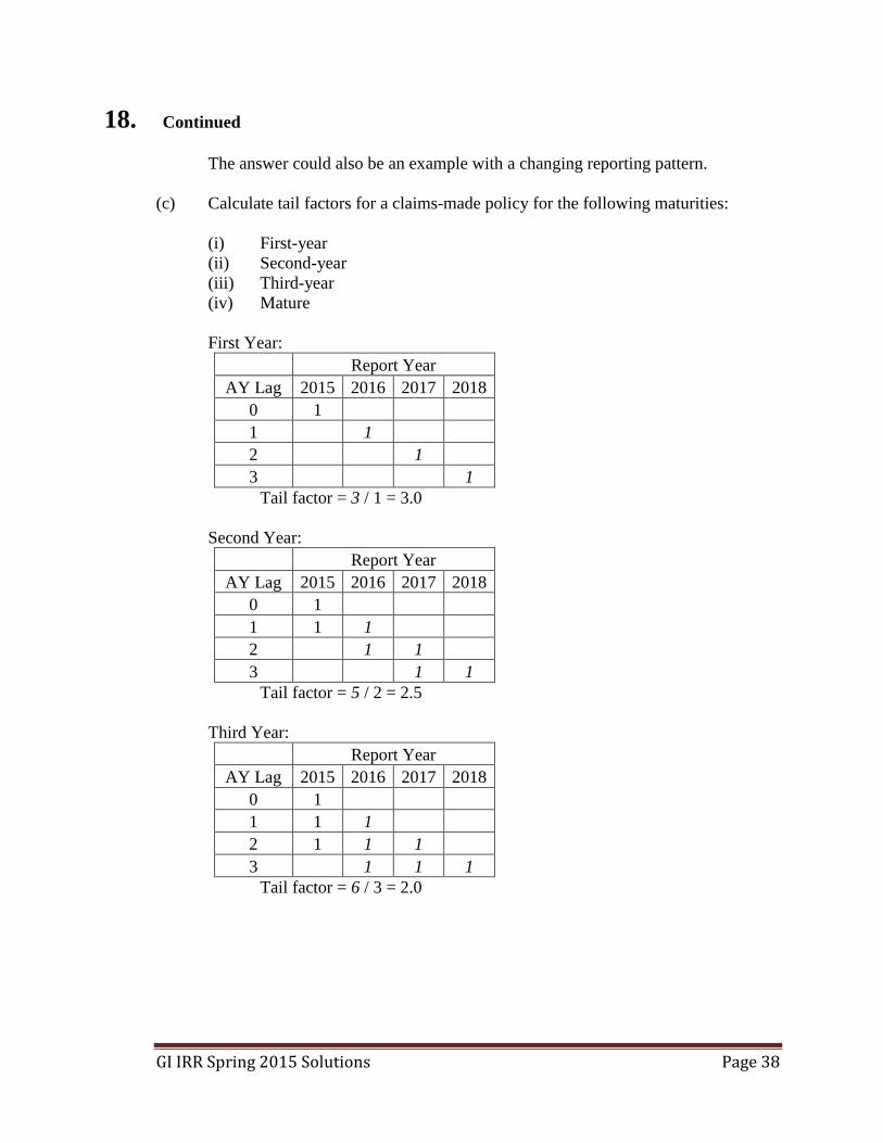
(c) Calculate tail factors for a claims-made policy for the following maturities:

(i) First-year

(ii) Second-year

(iii) Third-year

(iv) Mature

First Year:

Report Year

AY Lag 2015 2016 2017 2018

0 1

1 1

2 1

3 1

Tail factor = 3 / 1 = 3.0

Second Year:

Report Year

AY Lag 2015 2016 2017 2018

0 1

1 1 1

2 1 1

3 1 1


Third Year:

Report Year

AY Lag 2015 2016 2017 2018

0 1

1 1 1

2 1 1 1

3 1 1 1



18. Continued

Fourth Year:

Report Year

AY Lag 2015 2016 2017 2018

0 1

1 1 1

2 1 1 1

3 1 1 1 1


(d) Determine the earned premium in 2015, 2016 and 2017 for a mature tail policy

effective January 1, 2015 with a premium of 15,000.

With a 15,000 tail premium split into six units, the earning would be as follows:

2015: (3/6) of 15,000 = 7,500

2016: (2/6) of 15,000 = 5,000

2017: (1/6) of 15,000 = 2,500




Learning Outcomes:

(5g) Calculate risk classification changes and territorial changes.

Sources:



This question tests basic general insurance risk classification.

Solution:

(a) Describe three desirable attributes of a risk classification system.


Homogeneity: Risks within a risk class should be sufficiently homogeneous in

nature such that there are no clear identifiable subclasses within a risk class;

and therefore risks that are significantly dissimilar should belong to different

risk classes.

Objectivity: The definition of risk classes should be clear and objective.

Where possible, the evaluation of a risk characteristic should be factual and

not judgmental.

Cost: There should be a reasonable relationship between the cost of adding a

risk characteristic for classification purposes and the benefit of adding such

characteristic.

Verifiability: The risk characteristics used in a risk classification system

should be reliable and conveniently verifiable.

Other considerations: (a) comply with applicable law; (b) consider industry

practices for that type of financial or personal security system as known to the

actuary; and (c) consider limitations created by business practices of the

financial or personal security system as known to the actuary.

Reasonableness of the results: As with many types of actuarial work,

professional judgment plays an important role in the work supporting risk

classification systems.

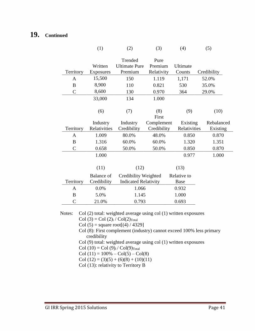
(b) Calculate the relativities to base Territory B using the pure premium approach.


19. Continued

(1) (2) (3) (4) (5)

Territory

Written

Exposures

Trended

Ultimate Pure

Premium

Pure

Premium

Relativity

Ultimate

Counts Credibility

A 15,500 150 1.119 1,171 52.0%

B 8,900 110 0.821 530 35.0%

C 8,600 130 0.970 364 29.0%

33,000 134 1.000

(6) (7) (8) (9) (10)

Territory

Industry

Relativities

Industry

Credibility

First

Complement

Credibility

Existing

Relativities

Rebalanced

Existing

A 1.009 80.0% 48.0% 0.850 0.870

B 1.316 60.0% 60.0% 1.320 1.351

C 0.658 50.0% 50.0% 0.850 0.870

1.000 0.977 1.000

(11) (12) (13)

Territory

Balance of

Credibility

Credibility Weighted

Indicated Relativity

Relative to

Base

A 0.0% 1.066 0.932

B 5.0% 1.145 1.000

C 21.0% 0.793 0.693

Notes: Col (2) total: weighted average using col (1) written exposures

Col (3) = Col (2)i / Col(2)Total

Col (5) = square root[(4) / 4329]

Col (8): First complement (industry) cannot exceed 100% less primary

credibility

Col (9) total: weighted average using col (1) written exposures

Col (10) = Col (9)i / Col(9)Total

Col (11) = 100% – Col(5) – Col(8)

Col (12) = (3)(5) + (6)(8) + (10)(11)

Col (13): relativity to Territory B


19. Continued

(c) Recommend three approaches to increase the stability of risk class relativities.


Use capped claims instead of total claims.

Use the territory with the highest exposure for the base relativity.

Use a longer experience period.

Increase the credibility standard (give more weight to the industry).

Give greater weight to existing relativities.

Use statistical tools to assess predictive stability.




Learning Outcomes:

(5d) Calculate loadings for catastrophes and large claims.

Sources:



This question tests the understanding of claim loadings for ratemaking.

Solution:

(a) Describe the difference between large claims and catastrophe claims.

Catastrophes typically result in a significant number of GI claims for multiple

insurers providing coverage in the area affected by the event.

Large claims do not typically affect the entire GI industry, or even all GI

companies operating in a specific area, but rather one or only a few policyholders

for one insurer.

(b) Calculate the hail loading for State X expressed as a claim ratio.

Average accident date in forecast period = June 1, 2016.

Trending period for accident year 2014 is from July 1, 2014 to June 1, 2016, or 23

months.

Average Accident Date

Accident

Year

Experience

Period

Forecast

Period

# of

months

trend

Severity

Trend at

7%

Hail

Ultimate

Claims

Trended

Hail

Ultimate

Claims

2010 July 1, 2010 June 1, 2016 71 1.4923 111,000 165,644

2014 July 1, 2014 June 1, 2016 23 1.1385 550,000 626,155

791,799


20. Continued

(1) Selected hail ultimate claims 791,799

(2) Total earned house years 2010 through 2014 72,452

(3) Trended pure premium for hail claims (1) / (2) 10.929

(4) CY 2014 earned house years 14,850

(5) Hail expected claims (3)(4) 162,290

(6) CY 2014 trended earned premium at current rate level 10,335,000

(7) Catastrophe hail loading expressed as a claim ratio (5) / (6) 1.57%

(c) Recommend the catastrophe hail loading for State X. Justify your answer.

The experience in State X does not seem credible and could be ignored.

The model matches the insurance experience when the exposure is significant,

suggesting a reasonable model.

Therefore, the model estimate for X of 3.4% is reasonable.

Documents

GI IRR Model Solutions - Society of Actuaries · GI IRR Model Solutions Spring 2015 1. Learning Objectives: 1. The candidate will understand the key considerations for general insurance