Embed Size (px)
Citation preview

Ghent University, Department of Applied Mathematics, Computer Science and Statistics
Hedging and pricing of life insurance portfolios
Helene De Coninck
promotor: Prof. dr. M. Vanmaele
Thesis written to obtain a Master in Science in Mathematics:Applied Mathematics.
Academic Year: 2014-2015


Ghent University, Department of Applied Mathematics, Computer Science and Statistics
Hedging and pricing of life insurance portfolios
Helene De Coninck
promotor: Prof. dr. M. Vanmaele
Thesis written to obtain a Master in Science in Mathematics:Applied Mathematics.
Academic Year: 2014-2015


Preface
This thesis has been written with help from my promotor Prof. dr. M. Vanmaele. So specialthanks to her for all her tips and comments.Further I would like to thank her for first interesting me in the subject of financial mathematics.After attending her course “Financiele Wiskunde” in the second year of my education, I knewthe direction I wanted to go next. After achieving a Bachelor in Mathematics, the choice of aMaster in Applied Mathematics was easily made. To further deepen myself in the world of in-surance and financial mathematics I opted for the minor Economics and Insurance. Ultimately,all of it has led to writing this thesis.
I also would like to express my gratitude to my math teachers in high school, who first in-troduced me into the world of mathematics.Acknowledgment should go to all professors of Mathematics at Ghent University for givingtheir students such a broad knowledge about the matter as well as teaching us to be critical andindependent. We have not just learned definitions, theorems, lemmas and proofs by heart; wehave learned to work logically, structural and efficient, making fact-based conclusions, usingwhat already is at hand. As Gyorgy Polya1 once has said:
“Mathematics is being lazy. Mathematics is letting the principles do the work for you so thatyou do not have to do the work yourself”.
I also want to thank my parents for giving me the chance to develop myself as a person, forletting me choose my own directions in life and for supporting me through my years of study,both financially as mentally. They have done a wonderful job on raising my sister and me.
1Gyorgy Polya was a Hungarian mathematician born December 13, 1887 and died September 3, 1985 at theage of 97.
v

As author I give permission so that this thesis can be used for consultation and so that parts ofthis thesis may be copied for personal use only. Any other use falls directly under the limita-tions of the copyright, particularly one has the obligation to mention the source explicitly whenreferring to results in this thesis.
Date: Sunday 31st May, 2015 Signature: De Coninck, Helene
vi
Contents
1 Introduction 1
2 The basics of stochastic calculus 3
3 The risk-minimizing theory 153.1 The basics . . . . . . . . . . . . . . . . . . . . . . . . . . . . . . . . . . . . . 153.2 The discrete-time trading case . . . . . . . . . . . . . . . . . . . . . . . . . . 163.3 The continuous-time trading case . . . . . . . . . . . . . . . . . . . . . . . . . 193.4 The mixed continuous-discrete-time trading case . . . . . . . . . . . . . . . . 243.5 Comparison . . . . . . . . . . . . . . . . . . . . . . . . . . . . . . . . . . . . 303.6 Reconsideration of the GKW decomposition . . . . . . . . . . . . . . . . . . . 33
4 An affine stochastic mortality model 374.1 The setting . . . . . . . . . . . . . . . . . . . . . . . . . . . . . . . . . . . . 374.2 The insurance contract . . . . . . . . . . . . . . . . . . . . . . . . . . . . . . 444.3 The survivor swap . . . . . . . . . . . . . . . . . . . . . . . . . . . . . . . . . 574.4 The risk-minimization theory applied to survivor swaps . . . . . . . . . . . . . 604.5 Comparison of the risk . . . . . . . . . . . . . . . . . . . . . . . . . . . . . . 66
5 A Heath-Jarrow-Morton stochastic mortality model 695.1 The setting . . . . . . . . . . . . . . . . . . . . . . . . . . . . . . . . . . . . 695.2 The insurance contract . . . . . . . . . . . . . . . . . . . . . . . . . . . . . . 735.3 The longevity bond . . . . . . . . . . . . . . . . . . . . . . . . . . . . . . . . 755.4 The risk-minimizing theory applied to longevity bonds . . . . . . . . . . . . . 845.5 The risk . . . . . . . . . . . . . . . . . . . . . . . . . . . . . . . . . . . . . . 91
6 Pricing theories 946.1 The pricing measure . . . . . . . . . . . . . . . . . . . . . . . . . . . . . . . 946.2 The indifference pricing theory . . . . . . . . . . . . . . . . . . . . . . . . . . 99
7 A mortality intensity model 1037.1 The setting . . . . . . . . . . . . . . . . . . . . . . . . . . . . . . . . . . . . 1037.2 The longevity risk price through the pricing measure . . . . . . . . . . . . . . 1127.3 The longevity risk price through indifference pricing . . . . . . . . . . . . . . 1147.4 Comparison . . . . . . . . . . . . . . . . . . . . . . . . . . . . . . . . . . . . 122
8 Conclusion 124
vii

CONTENTS
A Nederlandstalig samenvatting 127
B Proof second equality page 31-32 130
C Proof of Proposition 4.3.1 131
D Cramer’s method for Theorem 4.4.1 132
viii Pricing and hedging of life insurance portfolios H. De Coninck
List of Figures
2.1 A point process and its counting process, taken from Bremaud (1981). . . . . . 62.2 A three-variate point process and its counting process, taken from Bremaud
(1981). . . . . . . . . . . . . . . . . . . . . . . . . . . . . . . . . . . . . . . . 6
6.1 A quadratic utility (A = 3.25). . . . . . . . . . . . . . . . . . . . . . . . . . . 1006.2 A power utility (R = 0.75). . . . . . . . . . . . . . . . . . . . . . . . . . . . . 1006.3 An exponential utility (γ = 5). . . . . . . . . . . . . . . . . . . . . . . . . . . 101
ix

Chapter 1
Introduction
In the world of today insurance is very important. They allow people to transfer their own riskin return for a price. This price can be a purchase price, which has to be paid only once, butone can also opt for periodical payments, called premiums. The price is paid by the insuredto either a person or company, called the insurer. In general one can choose freely to take onan insurance for a given price. In some cases however, insurance is compulsory. Think ofmotor insurance, employer’s liability (also known as occupational accident insurance effectedby employers) or insurance that is mandatory in the scope of the exercised activities, such ashunting policies, professional liability insurance et cetera1. We should note that despite thefact these insurance policies are compulsory, one is still allowed to choose the insurer. Othertypes of insurance are optional such as legal expenses insurance, life insurance, private healthinsurance, third party fire and theft car insurance, hail insurance and so on. Besides being nolonger responsible for the consequences of the risks you have insured, insurance can also haveother advantages. Life insurance, for example, can be an alternative manner of saving (insteadof depositing your money at a bank account, you could invest it in a life insurance). If one isalive when the contract terminates, you receive a capital. So this type of insurance can be seenas an investment of money, that at the end pays you back a certain amount. Some policies havefiscal advantages, which makes them more attractive than other investment options.
While the insured is disposed of his risk, the insurer has to be able to handle the prospect-ive risk. Since you can never tell for sure whether a risk will unfold or when it will happen,undertaking risk is relatively unpredictable. Throughout the years different methods, modelsand rules have been set up, trying to make realistic predictions about risk occurrences, abouthow much money they will cost the insurer, what kind of catastrophes may happen and whatthe impact will be on the insurer’s position,...One important feature of selling insurance contracts, is that the insurer has to be able to meet hisliabilities. In order to do so, the insurer will first have to determine correct prices for his con-tracts. This means that one needs to ask premiums or purchase prices which are high enough tocover the accepted risks. On the other hand the insurer must maintain sufficiently low prices sothat people will keep on buying those products and not the ones from the competition. Secondly,the money the insurer receives has to be invested properly in order to cover the (future) liab-ilities, as well as other costs that come with running an insurance business. This, in general,
1If you wish more information about this topic, you can always contact the FOD (Federal Government Service)or the FSMA (Financial Services and Markets Authority) or visit their websites.
1
CHAPTER 1. INTRODUCTION
is also referred to as hedging and can be done in many different ways. The most basic wayis to deposit money at a bank so that over time it accrues interest. Other options are to investin assets such as bonds, real estate, shares, commodities or derivatives. Depending on the typeof product, the investment can have a higher return but this will be at the expense of a higher risk.
In this thesis we will only consider life insurance contracts and focus on the two aspects men-tioned in the previous paragraph, namely the hedging and pricing. The first (and biggest) partwill cover the hedging. To begin with, we give an introduction to the risk-minimizing theorywhich will be used to derive the hedging formulas. We will discuss three trading settings: thediscrete-time trading case, the continuous-time trading case and the mixed continuous-discrete-time trading case. Chapters 4 and 5 start with describing a market setting, after which theexplanation of an insurance contract and a financial instrument follows. To the latter we thenapply the risk-minimizing theory. At the basis of chapters 3 to 5 are the papers of Dahl et al.(2011), Dahl et al. (2008), Follmer and Schweizer (1989) and Barbarin (2008).The contracts we will consider, are relatively simple. Nowadays, a lot of variations on suchcontracts can be made, allowing for different payments depending on the situation. Differencescan also arise in premiums and interest rates. They can be fixed, variable, (not) guaranteed orguaranteed until a certain level and so one. Some policies allow for profit sharing. Dependingon the profit, the insurer pays the contract holders an additional sum of money. On top of thatone can often include several options in the contract, making it more tailor made.
Chapter 6 gives again an introduction, but about pricing theories. We will highlight two differ-ent strategies in pricing: the equivalent martingale measure and the indifference pricing theory.The first method is widely known and frequently used in scientific literature. The second methodoriginates from a more economic perspective, but is also quite often used in papers. Many morecan be considered, though. For example, one could apply the well known Markowitz theory. Inthe work of Kahane (1979) one can find the application of this method along with advantagesand disadvantages. One can also use premium principles, where one derives a functional basedon a set of given axioms that premiums should follow. More details can be found in Tsanakasand Desli (2005). In chapter 7 we apply both theories to a simplified setting and we comparetheir outcomes. The pricing part is mainly based on Hainaut and Devolder (2008).The thesis will end with a conclusion about the methods used. In the appendix that follows, onecan find a brief summary of this thesis in Dutch.
2 Pricing and hedging of life insurance portfolios H. De Coninck
Chapter 2
The basics of stochastic calculus
Before we bring up the actual subject of this thesis, we give a more informative chapter. Theidea is to bring forward a couple of basics of stochastic calculus as well as introducing conceptsthat will be used throughout this work.
In general we work in a probability space (Ω,F ,P), where Ω is the space of all possible out-comes, F is a σ-algebra on Ω and P a probability measure. We call F the corresponding filtra-tion. The time interval that we will work on is defined by [0,T ] with T strictly positive.First we introduce some definitions and widely known concepts which can be found in Contand Tankov (2004), Dahl et al. (2011), Follmer and Sondermann (1986), Protter (2004), Jacodand Shiryaev (2003), Bremaud (1981) and Joshi (2008).
Definition 2.0.1A process X(t)t∈[0,T ] is called F-measurable if for all t ∈ [0,T ], X(t) is known conditional onF (t).
We also say that X(t)t∈[0,T ] is F-adapted or F-non-anticipating.
Definition 2.0.2A process X(t)t∈[0,T ] is called predictable if it isP-measurable whereP is a σ-algebra generatedby all F-measurable, left-continuous processes on [0,T ] ×Ω.
Definition 2.0.3A random variable τ is called an F (t)-stopping time if for every t ∈ [0,T ], you have thatτ ≤ t ∈ F (t).
The above definition means that F (t) contains enough information to determine whether a cer-tain event, characterized by the random variable τ, has occurred or not. Or thus for everyt ∈ [0,T ] we know whether τ ≤ t ∈ F (t) or not.
Definition 2.0.4A function f is called cadlag1 if it is right-continuous and has (a) left limit(s).
An analogue definition can be made for caglad.
1The word cadlag is an abbreviation of the French “continu a droite, limite a gauche”.
3
CHAPTER 2. THE BASICS OF STOCHASTIC CALCULUS
Consider an investment portfolio with value process X(t)t∈[0,T ] and with D(t)t∈[0,T ] the discount-ing process. We have that
d(DX)(t) = D(t)dX(t) + X(t)dD(t) + dD(t)dX(t),
because of the chain rule. In some cases this expression can be simplified.
Proposition 2.0.1Assume an investment portfolio with value process X(t)t∈[0,T ] generates a cash flow C(t)t∈[0,T ]
which is F-adapted, then the dynamics of the discounted value process (DX)(t)t∈[0,T ] are givenby
d(DX)(t) = D(t)dC(t),
for every t ∈ [0,T ].
Definition 2.0.5A process M(t)t∈[0,T ] is a local martingale if there exists an increasing sequence of stoppingtimes (Tn)n≥0 such that lim
n→+∞Tn = +∞ almost surely and each stopped process M(t∧ Tn)t∈[0,T ] is
again a martingale.
Note that every martingale is a local martingale but the inverse does not necessarily hold.
Definition 2.0.6A process M(t)t∈[0,T ] is called a semimartingale if, for every t ∈ [0,T ], M(t) can be written as
M(t) = M(t) + A(t),
with M(t)t∈[0,T ] a local martingale that has a finite starting value M(0) and A(t)t∈[0,T ] an adapted,real-valued cadlag process that satisfies A(0) = 0 and has a finite variation.
This decomposition is not necessarily unique, but if we can find a process A(t)t∈[0,T ] that fulfillsthe conditions in the previous definition and is F-predictable then we call
(M + A
)(t)t∈[0,T ] the
canonical decomposition of M(t)t∈[0,T ]. Since there is at most one process just described, thecanonical decomposition is unique if we can find such a process A(t)t∈[0,T ].
Definition 2.0.7Consider a process X(t)t∈[0,T ] with finite variation. There exists a unique, increasing, F-predictableprocess A(t)t∈[0,T ] such that (X − A)(t)t∈[0,T ] is a local martingale. This process A(t)t∈[0,T ] is thecompensator of X.
The quadratic variation process of a process X(t)t∈[0,T ] is denoted by the bracket process [X, X](t)t∈[0,T ]
and is widely used. But there also exists an angle-bracket process 〈X, X〉 (t)t∈[0,T ], which givesthe conditional quadratic variation of X. This process is defined as the compensator of [X, X].
Proposition 2.0.2Let X(t)t∈[0,T ] be a semimartingale, then
[X, X](t)t∈[0,T ] = [X, X]c (t)t∈[0,T ] +∑
0≤s≤t
(∆X)2(s)
= 〈Xc, Xc〉 (t)t∈[0,T ] +∑
0≤s≤t
(∆X)2(s),
where [X, X]c is the continuous part of [X, X], Xc is the continuous local martingale part of Xand the last term forms the discontinuous part, being the jumps.
4 Pricing and hedging of life insurance portfolios H. De Coninck
CHAPTER 2. THE BASICS OF STOCHASTIC CALCULUS
Note that if X(t)t∈[0,T ] is continuous and X(0) = 0, we get the following equality:
[X, X](t)t∈[0,t] = [X, X]c(t)t∈[0,T ] = 〈Xc, Xc〉 (t)t∈[0,T ] = 〈X, X〉 (t)t∈[0,T ].
One of the most used formulas in stochastic mathematics is the Ito formula:
f (t,W(t))
= f (0,W(0)) +
∫ t
0
∂
∂sf (s,W(s))ds +
∫ t
0
∂
∂xf (s,W(s))dW(s) +
12
∫ t
0
∂2
∂x2 f (s,W(s))d[W,W](s),
where f : [0,T ] × R → R is a sufficiently differentiable function and W(t)t∈[0,T ] is a Brownianmotion under P.If X(t)t∈[0,T ] is a semimartingale, we can still make use of the above expression, but in a slightlyaltered form.
Theorem 2.0.1 (Ito formula for semimartingales)Let X(t)t∈[0,T ] be a semimartingale and f : [0,T ]×R→ R a sufficiently differentiable, continuousfunction, then we have that
f (t, X(t)) = f (0, X(0)) +
∫ t
0
∂
∂sf (s, X(s))ds +
∫ t
0
∂
∂xf (s, X(s−))dX(s)
+12
∫ t
0
∂2
∂x2 f (s, X(s))d [X, X]c (s) +∑
0≤s≤t∆X(s),0
(∆ f (s, X(s)) − ∆X(s)
∂
∂xf (s, X(s−))
),
with [X, X]c the continuous part of [X, X] and ∆ f (s, X(s)) = f (s, X(s))− f (s, X(s−)) and ∆X(s) =
X(s) − X(s−).
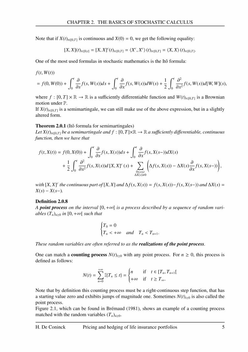
Definition 2.0.8A point process on the interval [0,+∞[ is a process described by a sequence of random vari-ables (Tn)n≥0 in [0,+∞[ such thatT0 = 0
Tn < +∞ and Tn < Tn+1.
These random variables are often referred to as the realizations of the point process.
One can match a counting process N(t)t≥0 with any point process. For n ≥ 0, this process isdefined as follows:
N(t) =
+∞∑n=0
ITn ≤ t =
n if t ∈ [Tn,Tn+1[+∞ if t ≥ T∞.
Note that by definition this counting process must be a right-continuous step function, that hasa starting value zero and exhibits jumps of magnitude one. Sometimes N(t)t≥0 is also called thepoint process.Figure 2.1, which can be found in Bremaud (1981), shows an example of a counting processmatched with the random variables (Tn)n≥0.
H. De Coninck Pricing and hedging of life insurance portfolios 5
CHAPTER 2. THE BASICS OF STOCHASTIC CALCULUS
Figure 2.1: A point process and its counting process, taken from Bremaud (1981).
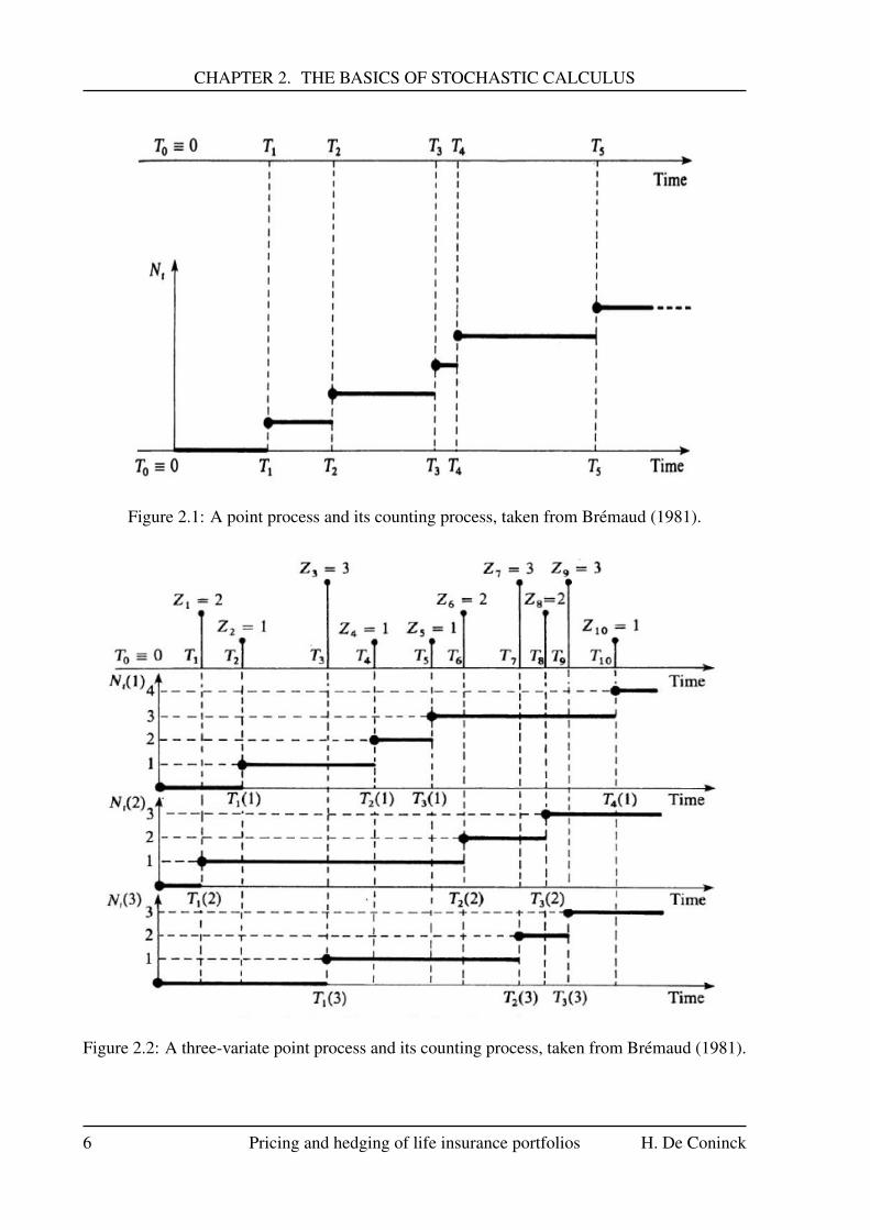
Figure 2.2: A three-variate point process and its counting process, taken from Bremaud (1981).
6 Pricing and hedging of life insurance portfolios H. De Coninck

CHAPTER 2. THE BASICS OF STOCHASTIC CALCULUS
Definition 2.0.9A k-variate point process on a probability space (Ω,F ,P) is described by two sequences ofrandom variables (Tn,Zn)n≥0 such that:
• (Tn)n≥0 is a point process as in Definition 2.0.8,
• (Zn)n≥0 is a sequence that takes up values in the set 1, . . . , k.
For 1 ≤ x ≤ k and t ≥ 0, the corresponding counting process N(t, x)t≥0 is given by
N(t, x) =
+∞∑n=0
ITn ≤ tIZn = x.
Figure 2.2, which can be found in Bremaud (1981), shows a three-variate point process with itscorresponding counting process.
Definition 2.0.10An E-marked point process is a process described by a sequence of random variables (Tn,Zn)n≥0,with (Tn)n≥0 being a time-related random variable and (Zn)n≥0 being a magnitude-related ran-dom variable with values in the set E. This space E is called the mark space.If E = 1, . . . , k, we just have a k-variate point process (recall Definition 2.0.9).
The corresponding counting process is again
N(t, x) =
+∞∑n=0
ITn ≤ tIZn = x,
where now, x is an element in E.
Proposition 2.0.3A point process is P-non explosive if T∞ = lim
n→+∞Tn = +∞, which is equivalent with, for every
t ≥ 0, N(t) < +∞ P-almost surely.
Proposition 2.0.3 can be extended for k-variate point processes. We note that if the expectedvalue of the counting process is bounded, it is also integrable.
Definition 2.0.11A random variable X has a Poisson distribution with parameter λ if for all x in N (zero in-cluded) we have that
PX = x =e−λλx
x!.
If a random variable X is Poisson distributed with parameter λ, we write this as X ∼ P(λ).
Definition 2.0.12If a counting process N(t)t∈[0,T ] fulfills the following conditions:
1. for every t ∈ [0,T ] we have that N(t) is F (t)-adapted,
2. N(t)t∈[0,T ] has independent increments,
H. De Coninck Pricing and hedging of life insurance portfolios 7

CHAPTER 2. THE BASICS OF STOCHASTIC CALCULUS
3. N(t)t∈[0,T ] has stationary2 increments,
then N(t)t∈[0,T ] is called a Poisson process.
Proposition 2.0.4If N(t)t∈[0,T ] is a Poisson process, then there exists a λ ≥ 0 such that, for all t ∈ [0,T ], N(t) isPoisson distributed with parameter λt.This λ is called the intensity associated with the Poisson process N(t)t∈[0,T ].
Poisson processes have a couple of interesting properties. One that is often used, is that (N(t) −λt)t∈[0,T ], which is called the compensated Poisson process, is a martingale. Another propertyis given below.
Proposition 2.0.5If N(t)t∈[0,T ] is a Poisson process, then we have the next equalities for all t ∈ [0,T ]:
[N,N](t) = N(t) and 〈N,N〉 (t) = λt.
We also have that [N − λ,N − λ](t) = N(t). Note that the first equality in Proposition 2.0.5 isalso valid when N(t)t∈[0,T ] is just a counting process.
Definition 2.0.13Two random variables X and Y with finite variances are called orthogonal if E[XY] = 0.
In light of the previous definition we say that a random variable is orthogonal to a set if it isorthogonal to all random variables in this set.
Definition 2.0.14Two square-integrable (local) martingales are called orthogonal if their product is again a(local) martingale.
The definition of orthogonality of two martingales M1(t)t∈[0,T ] and M2(t)t∈[0,T ] is equivalent tothe following condition:
[M1,M2] = 0.
An important theorem that will be used frequently is the Galtchouk-Kunita-Watanabe decom-position. The theorem can by found in Cont and Tankov (2004). When referring to this theoremwe will use the abbreviation GKW instead of writing Galtchouk-Kunita-Watanabe.
Theorem 2.0.2 (Galtchouk-Kunita-Watanabe decomposition)Let M(t)t∈[0,T ] be a square-integrable martingale with respect to the equivalent martingale meas-ureQ. Any random variable H with finite variance depending on the history of M(t)t∈[0,T ] can berepresented as the sum of a stochastic integral with respect to M(t)t∈[0,T ] and a random variableNH, such that the martingale NH(t)t∈[0,T ] =
(EQ
[NH
∣∣∣F (t)])
t∈[0,T ]is orthogonal with respect to
M(t)t∈[0,T ].In other words, there exists a square-integrable, predictable process ϕ such that with probabilityone
H = EQ [H] +
∫ T
0ϕ(s)dM(s) + NH.
2We call increments stationary if the distribution of the increments is dependent on the length of the increments.Thus, if s ≤ t, k ≤ l and t − s = l − k then X(t) − X(s) should equal X(l) − X(k) in distribution.
8 Pricing and hedging of life insurance portfolios H. De Coninck

CHAPTER 2. THE BASICS OF STOCHASTIC CALCULUS
In particular, for any square-integrable, predictable process γ(t)t∈[0,T ],(NH(t)
∫ t
0γ(s)dM(s)
)t∈[0,T ]
is again a martingale.
Note that with “history” we mean all past values that the process has taken up since the startuntil the current moment, completed with all null sets.
We also state the next proposition, which will be frequently used.
Proposition 2.0.6Let X(t)t∈[0,T ] be a cadlag, square-integrable martingale and let ψ(t)t∈[0,T ] be a bounded, pre-
dictable process. Then∫ t
0ψ(s)dX(s) is also a square-integrable martingale.
Its local analogue is given by the next proposition.
Proposition 2.0.7Let X(t)t∈[0,T ] be a local martingale and ψ(t)t∈[0,T ] a locally bounded, predictable process. Then∫ t
0ψ(s)dX(s) is a local martingale.
Another important part of this thesis relies on Levy processes. We will give some importantdefinitions and features. For more details about these processes and their properties see Contand Tankov (2004), Applebaum (2004), Kuchler and Sørensen (1997) and Di Nunno et al.(2009).
Definition 2.0.15Let X be a random variable with distribution FX and u ∈ R. The moment generating functionof X is the function
φX(u) = E[euX
]=
∫ +∞
−∞
euxdFX(x).
In most literature mgf is used as the abbreviation for moment generating function. We will alsouse this notation.The mgf is of importance since taking the nth derivative with respect to u and then setting uzero, provides you with the nth moment. In particular, it is easy to find the mean and variance ifyou know the mgf.
Definition 2.0.16Let X be a random variable with distribution FX and u ∈ R, then
φX(iu) = E[eiuX
]=
∫ +∞
−∞
eiuxdFX(x)
is called the characteristic function of X.
One should note that the i in the previous definition is the irrational number i.
If a variable is Poisson distributed, then we have the following expression for the mgf (seeDefinitions 2.0.11 and 2.0.15). For the characteristic function an analogue expression can befound by using Definition 2.0.16.
φX(u) = E[euX
]H. De Coninck Pricing and hedging of life insurance portfolios 9
CHAPTER 2. THE BASICS OF STOCHASTIC CALCULUS
=
+∞∑x=0
eux fX(x) Poisson is a discrete distribution
=
+∞∑x=0
eux e−λλx
x!
= e−λ+∞∑x=0
(euλ)x
x!
= e−λeλeuseries expansion of e
= exp λ (eu − 1) .
Definition 2.0.17Let X(t)t∈[0,T ] be a stochastic process. If the following conditions are satisfied, we say thatX(t)t∈[0,T ] is a Levy process:
1. X(0) = 0 almost surely,
2. X(t)t∈[0,T ] has independent increments,
3. X(t)t∈[0,T ] has stationary increments,
4. X(t)t∈[0,T ] is stochastically continuous: (∀ε > 0) (∀s ≥ 0)(limt→sP |X(t) − X(s)| > ε = 0
).
A well known example of a Levy process is the Brownian motion. This is clear from its defini-tion, see for example Shreve (2004b).
Definition 2.0.18Let X(t)t∈[0,T ] be a Levy process and u ∈ R, then the characteristic function of X(t)t∈[0,T ] isdefined by
φX(t)(iu) = E[eiuX(t)
].
An analogue definition can be given for the mgf of X(t)t∈[0,T ].
The mgf and the characteristic function are related to one another:
φX(t)(u) = E[euX(t)
]by Definition 2.0.18
= E[e−i2uX(t)
]= φX(t)(i(−iu)).
By the previous relationship and because you can calculate the nth moment from the mgf, itis easy to see that by taking the nth derivative with respect to u of the characteristic function,dividing by in and then choosing u = 0, you also get the nth moment.
Definition 2.0.19For a Levy process X(t)t∈[0,T ] and u ∈ R we define the cumulant transform k as follows:
k(u) = ln E[exp uX(1)
]= ln φX(1)(u).
Before giving two of the most important theorems in connection with Levy processes: the Levy-Ito decomposition (Theorem 2.0.3) and the Levy-Khintchine representation (Theorem 2.0.4),we introduce some important measures and properties.
10 Pricing and hedging of life insurance portfolios H. De Coninck
CHAPTER 2. THE BASICS OF STOCHASTIC CALCULUS
Definition 2.0.20Let (A,A) be a measurable space. A random measure ν on (A,A) is a collection of randomvariables ν(B)B∈A such that:
1. ν(∅) = 0,
2. (σ-additive)
for every disjoint sequence of sets (Bn)n∈N inA, we have that ν
⋃n∈N
Bn
=∑n∈N
ν(Bn),
3. (independent scattered property)the measures ν(B1), . . . , ν(Bn) are independent for every disjoint family of sets (Bi)i=1,...,ninA.
Definition 2.0.21If ν is a random measure on a measurable space (A,A), then we say that ν is a Poisson randommeasure if for every B ∈ A with ν(B) < +∞, ν(B) has a Poisson distribution.
Lets consider a Levy process X(t)t∈[0,T ]. Its jumps are denoted by (∆X(t))t∈[0,T ]. We can thenassociate a Poisson random measure which counts the number of jumps that have given size.For A ∈ B
(Rd \ 0
)we get JX(t, A) =
∑0≤s≤t
I∆X(s) ∈ A, where B(Rd \ 0
)is the Borel set of
Rd \ 0.We can now define νX(A) as E [JX(1, A)], which is called the intensity of the Poisson randommeasure JX. The compensated Poisson random measure is then defined as JX(t, A) − tνX(A).
Definition 2.0.22Let A be a set, B(A) its Borel σ-algebra and ν a random measure on [0,+∞[×A. For everyB ∈ B(A) define the process ν(t, B)t∈[0,T ] = ν([0, t[×B)t∈[0,T ]. If there exists an element C ∈ B(A)such that ν(t,C)t∈[0,T ] is a martingale under the condition that the disjunction of the closure ofB and C is empty, or thus B ∩C = ∅, then ν is called a martingale-valued measure.
Proposition 2.0.8The compensated Poisson random measure JX(t, A) − tνX(A) for a Levy process X(t)t∈[0,T ] and aset A is a martingale-valued measure, or thus tνX is the compensator of JX.
The Levy-Ito decomposition allows one to “split” up the Levy process into different compon-ents: a time-related component, a Brownian motion part and the integral terms, which aredependent on the associated Poisson random measure.
Theorem 2.0.3 (Levy-Ito decomposition)Consider a Levy process X(t)t∈[0,T ]. There exists a vector γ in Rd, a d-dimensional Brownian mo-tion W(t)t∈[0,T ] with covariance matrix Σ, an independent Poisson random measure JX, definedon [0,+∞[×Rd \ 0, and its intensity νX such that for all t ∈ [0,T ] we have that
X(t) = γt + W(t) +
∫|x|<1
x (JX(t, dx) − tνX(dx)) +
∫|x|≥1
xJX(t, dx).
The intensity in this theorem is also called the Levy measure.The elements γ, νX and Σ characterize the Levy process so therefore (γ, νX,Σ) is called thecharacteristic triplet of X(t)t∈[0,T ].
H. De Coninck Pricing and hedging of life insurance portfolios 11
CHAPTER 2. THE BASICS OF STOCHASTIC CALCULUS
While the above theorem gives a decomposition of the Levy process itself, the Levy-Khintchinerepresentation gives a way to split up the characteristic function of the process.
Theorem 2.0.4 (Levy-Khintchine representation)Let X(t)t∈[0,T ] be a Levy process on Rd with characteristic triplet (γ, νX,Σ) and u ∈ Rd. Thecorresponding characteristic function is given by
φX(t)(iu) = exp(
iγtru −12
utrΣu +
∫Rd
(eiutr x − 1 − iutr xI|x| ≤ 1
)νX(dx)
)t.
Proposition 2.0.9A Levy process is a semimartingale.
Definition 2.0.23If a one-dimensional stochastic process X(t)t∈[0,T ] has a stochastic integral representation of thefollowing form:
X(t) = x +
∫ t
0α(s)ds +
∫ t
0β(s)dW(s) +
∫ t
0
∫R\0
γ(s, y)(J(ds, dy) − ν(dy)ds),
where α(t)t∈[0,T ], β(t)t∈[0,T ] and γ(t, y)t∈[0,T ] are predictable processes such that for all t ∈ [0,T ]and y ∈ R\0∫ t
0
(|α(s)| + β2(s) +
∫R\0
γ2(s, y)ν(dy))
ds < +∞,P-almost surely,
then we call X(t)t∈[0,T ] an Ito-Levy process.
Just as for semimartingales, we can find an adjusted form of the Ito formula for Ito-Levy pro-cess.
Theorem 2.0.5 (Ito formula for Ito-Levy process)Let X(t)t∈[0,T ] be an Ito-Levy process and f : [0,T ] × R → R a sufficiently differentiable,continuous function, then we have that
f (t, X(t))
= f (0, X(0)) +
∫ t
0
∂
∂sf (s, X(s))ds +
∫ t
0α(s)
∂
∂xf (s, X(s))ds +
∫ t
0β(s)
∂
∂xf (s, X(s))dX(s)
+12
∫ t
0β2(s)
∂2
∂x2 f (s, X(s))ds
+
∫ t
0
∫R\0
(f (s, X(s) + γ(s, y)) − f (s, X(s)) −
∂
∂xf (s, X(s))γ(s, y)
)ν(dy)ds
+
∫ t
0
∫R\0
( f (s, X(s−) + γ(s, y)) − f (s, X(s−))) (J(ds, dy) − ν(dy)ds) .
The differential form of the previous theorem is given by
d f (t, X(t))
=∂
∂tf (t, X(t))dt + α(t)
∂
∂xf (t, X(t))dt + β(t)
∂
∂xf (t, X(t))dX(t) +
12β2(t)
∂2
∂x2 f (t, X(t))dt
12 Pricing and hedging of life insurance portfolios H. De Coninck
CHAPTER 2. THE BASICS OF STOCHASTIC CALCULUS
+
∫R\0
(f (t, X(t) + γ(t, y)) − f (t, X(t)) −
∂
∂xf (t, X(t))γ(t, y)
)νX(dy)dt
+
∫R\0
( f (t, X(t−) + γ(t, y)) − f (t, X(t−))) (JX(dt, dy) − νX(dy)dt) .
Definition 2.0.24A subordinator is a one-dimensional, almost surely non decreasing Levy process.
Subordinators form a special class of Levy processes and are often used since they have goodproperties, such as tractability. Within the class of subordinators, you can find different sub-classes, depending on their properties. A more known subclass is the one formed by the α-stablesubordinators.In chapter 7 we will go deeper into this type of processes.
Proposition 2.0.10A process X(t)t∈[0,T ] is a subordinator if and only if its characteristic triplet is given by (γ, νX, 0),with:
1. νX(] −∞, 0]) = 0,
2.∫ 1
0xνX(dx) < +∞,
3. γ ≥ 0.
Proposition 2.0.11Every subordinator is of finite variation.
Proposition 2.0.11 gives an important feature of subordinators. Due to the finite variation prop-erty, the Levy-Ito decomposition from Theorem 2.0.3 and Levy-Khintchine representation fromTheorem 2.0.4 can be reduced. The next theorem gives the formulations.
Theorem 2.0.6 (Levy-Ito and Levy-Khintchine in the finite variation case)Let X(t)t∈[0,T ] be a Levy process with characteristic triplet (γ, νX, 0) and finite variation. Letu ∈ Rd. Then we get
X(t) = bt +
∫Rd
xJX(t, dx)
and
φX(t)(iu) = exp
ibtrut + t∫Rd
(eiutr x − 1
)νX(dx)
,
where b = γ −
∫|x|<1
xνX(dx) is the drift.
Last, the theorem of Fubini, which gives the conditions for swapping integrals in a doubleintegration, is introduced.
Theorem 2.0.7 (Fubini)Consider a measure space (X×Y,X⊗Y, p×q) with (X×Y) the product space of the sets X andY, (X ⊗ Y) the product σ-algebra of the minimal σ-algebras X and Y and (p × q) the product
H. De Coninck Pricing and hedging of life insurance portfolios 13

CHAPTER 2. THE BASICS OF STOCHASTIC CALCULUS
measure of the measures p and q on the spaces (X,X) and (Y,Y) respectively.Let f : X × Y → R be a function that is either integrable or non negative, then we have∫
X
(∫Y
f (x, y)dq(y))
dp(x) =
∫X×Y
f (x, y)d(p × q)(x, y) =
∫Y
(∫X
f (x, y)dp(x))
dq(y).
We note that there exists several variants of Fubini’s theorem. One of them can be used to swapsummation with an integral given that the considered function is positive, or thus if, for all xand n ≥ 0, fn(x) ≥ 0 we have that∫ ∑
n
fn(x)dx =∑
n
∫fn(x)dx.
For further basics on stochastic calculus we refer to Shreve (2004a), Shreve (2004b), Cont andTankov (2004) and Bjork (2009).
14 Pricing and hedging of life insurance portfolios H. De Coninck
Chapter 3
The risk-minimizing theory
3.1 The basicsWe first note that throughout the first part of this thesis, the following definitions are used unlessstated otherwise. Most of it can be found in Dahl et al. (2011).
Our goal is to trade assets in the general setting, introduced in chapter 2, in such a way thatthe risk we are exposed to, is minimal. This boils down to finding a trading strategy that min-imizes the risk.Consider a setting that contains d + 1 assets with X(t)t∈[0,T ] the d-dimensional discounted priceprocess of the first d assets and Y(t)t∈[0,T ] the discounted price process of the last asset. Weassume that all necessary integrability conditions are satisfied. Assume further that we have asavings account B and a payment process A(t)t∈[0,T ] of the hedger.
Definition 3.1.1In agreement with proposition 2.0.1, the corresponding discounted payment process A∗(t)t∈[0,T ]
is given by
A∗(t) = A(0) +
∫ t
0B−1(s)dA(s).
Instead of working under the original P-measure, we assume that there is an equivalent martin-gale measure Q such that (X(t),Y(t))t∈[0,T ] is a (d + 1)-dimensional martingale.
Definition 3.1.2A strategy ϕ is a sufficiently integrable process ϕ(t)t∈[0,T ] = (ξ(t), ϑ(t), η(t))t∈[0,T ], where ξ(t)t∈[0,T ]
is a d-dimensional, F-predictable process that gives the number of the first d assets held,ϑ(t)tt∈[0,T ] is a one-dimensional, F-predictable process that gives the number of the last assetheld and η(t)t∈[0,T ] is a one-dimensional, F-adapted process giving the discounted deposit in thesavings account.
Definition 3.1.3The discounted value process V∗(t, ϕ)t∈[0,T ] associated with the trading strategy ϕ is defined by
V∗(t, ϕ) = ξ(t)X(t) + ϑ(t)Y(t) + η(t).
Definition 3.1.4The intrinsic value process V∗,Q(t)t∈[0,T ] is defined as
(EQ[A∗(T )|F (t)]
)t∈[0,T ]
, with A∗(t)t∈[0,T ] thediscounted payment process given in Definition 3.1.1.
15
CHAPTER 3. THE RISK-MINIMIZING THEORY
Definition 3.1.5A strategy ϕ is called x-admissible if the discounted value process has an end value x, in otherwords V∗(T, ϕ) = x.
Definition 3.1.6The cost process C(t, ϕ)t∈[0,T ] is defined by
C(t, ϕ) = V∗(t, ϕ) −∫ t
0ξ(s)dX(s) −
∫ t
0ϑ(s)dY(s) + A∗(t).
Definition 3.1.7The risk process R(t, ϕ)t∈[0,T ] is defined by
R(t, ϕ) = EQ[(C(T, ϕ) −C(t, ϕ))2
∣∣∣F (t)].
The theory of risk-minimization now states that a strategy ϕ is risk-minimizing if it minimizesthe risk process. This means that we have to find the strategy ϕ so that R(t, ϕ) is minimal for allt ∈ [0,T ].
In the remaining of this chapter we will briefly look at the discrete- and the continuous-timetrading case. Afterwards we will take a closer look at the mixed case, where we have bothdiscrete- and continuous-time trading.
3.2 The discrete-time trading caseThis section is mainly based on Follmer and Schweizer (1989).We consider a general setting but assume that all of our d + 1 assets can only be traded at fixedtimes in [0,T ]. We will denote these fixed trading times with 0 = t0 < t1 < . . . < tn−1 < tn = T .We now wish to find the optimal trading strategy ϕ(ti)i∈0,...,n = (ξ(ti), ϑ(ti), η(ti))i∈0,...,n, wherewe assume that ϕ is piecewise constant on each interval and F-measurable. We could just useone notation ϕ = (ξ, η) for all d + 1 assets, but we will not do so, in view of further comparison(see section 3.5). Note that for i = n, ξ(tn) and ϑ(tn) are zero since we stop our trading strategyat time T = tn. The theory of risk-minimization tells us that we can find the optimal strategy ϕby minimizing the risk process. In the discrete case the risk process is given by
R(ti, ϕ) = EQ[(C(ti+1, ϕ) −C(ti, ϕ))2
∣∣∣F (ti)],
with i = 0, . . . , n − 1.For simplicity we also assume that the covariance of the increments of X and Y terms are zero.
We will not make use of the discounted payment process from section 3.1. Instead we work witha payoff H such that the discounted value process V∗(ti, ϕ)i=0,...,n and cost process C(ti, ϕ)i=0,...,n
in the discrete setting reduce to:V∗(0, ϕ) = η(0)V∗(ti, ϕ) = ξ(ti−1)X(ti) + ϑ(ti−1)Y(ti) + η(ti), i = 1, . . . , n − 1V∗(tn, ϕ) = V∗(T, ϕ) = H,
16 Pricing and hedging of life insurance portfolios H. De Coninck
CHAPTER 3. THE RISK-MINIMIZING THEORY
andC(0, ϕ) = V∗(0, ϕ) = η(0)
C(ti, ϕ) = V∗(ti, ϕ) −i∑
j=1
ξ(t j−1) (X(t j) − X(t j−1))︸ ︷︷ ︸∆X(t j)
−
i∑j=1
ϑ(t j−1) (Y(t j) − Y(t j−1))︸ ︷︷ ︸∆Y(t j)
, i = 1, . . . , n.
We want (ξ(ti), ϑ(ti), η(ti))i=0,...,n to minimize the conditional risk, thus
minϕR(ti, ϕ) = min
ϕ
EQ
[(C(ti+1, ϕ) −C(ti, ϕ))2
∣∣∣F (ti)]
= minϕ
EQ
[(V∗(ti+1, ϕ) −
i+1∑j=1
(ξ(t j−1)∆X(t j) + ϑ(t j−1)∆Y(t j)
)− V∗(ti, ϕ) +
i∑j=1
(ξ(t j−1)∆X(t j) + ϑ(t j−1)∆Y(t j)
) )2∣∣∣∣∣∣F (ti)
]= min
ϕ
EQ
[(V∗(ti+1, ϕ) − V∗(ti, ϕ) − ξ(ti)∆X(ti+1) − ϑ(ti)∆Y(ti+1))2
∣∣∣F (ti)].
The idea is to choose V∗(ti, ϕ) (because we can calculate η(ti) using the solutions for V∗(ti, ϕ),ξ(ti−1) and ϑ(ti−1)), ξ(ti) and ϑ(ti) such that we achieve this minimum. In order to do so, we haveto calculate the first order conditions. Thus by taking the derivatives with respect to V∗(ti, ϕ),ξ(ti) and ϑ(ti) and solving them, we can solve the minimization problem. We first start with thederivation with respect to ξ(ti):
∂
∂ξ(ti)EQ
[(V∗(ti+1, ϕ) − V∗(ti, ϕ) − ξ(ti)∆X(ti+1) − ϑ(ti)∆Y(ti+1))2
∣∣∣F (ti)]
= 0
⇔ EQ[2 (V∗(ti+1, ϕ) − V∗(ti, ϕ) − ξ(ti)∆X(ti+1) − ϑ(ti)∆Y(ti+1)) (−∆X(ti+1))
∣∣∣F (ti)]
= 0
⇔ EQ[∆X(ti+1)
(V∗(ti+1, ϕ) − V∗(ti, ϕ)︸ ︷︷ ︸
F (ti)-measurable
− ξ(ti)︸︷︷︸F (ti)-measurable
∆X(ti+1) − ϑ(ti)︸︷︷︸F (ti)-measurable
∆Y(ti+1))∣∣∣F (ti)
]= 0
⇔ EQ[∆X(ti+1)V∗(ti+1, ϕ)|F (ti)
]− V∗(ti, ϕ)EQ
[∆X(ti+1)|F (ti)
]− ξ(ti)EQ
[(∆X(ti+1))2
∣∣∣F (ti)]
− ϑ(ti)EQ [∆X(ti+1)∆Y(ti+1)|F (ti)] = 0.
Since X(t)t∈[0,T ] is a Q-martingale, its expectation conditional on F (ti) is just X(ti). Thereforewe have that EQ[∆X(ti+1)|F (ti)] = 0:
EQ[∆X(ti+1)V∗(ti+1, ϕ)|F (ti)
]− V∗(ti, ϕ) EQ
[∆X(ti+1)|F (ti)
]︸ ︷︷ ︸0
−ξ(ti)EQ[(∆X(ti+1))2
∣∣∣F (ti)]
− ϑ(ti)EQ [∆X(ti+1)∆Y(ti+1)|F (ti)] = 0
⇔ ξ(ti)(EQ
[(∆X(ti+1))2
∣∣∣F (ti)]−
(EQ [∆X(ti+1)|F (ti)]
)2︸ ︷︷ ︸0
)= EQ
[∆X(ti+1)V∗(ti+1, ϕ)|F (ti)
]− EQ [∆X(ti+1)|F (ti)] EQ
[V∗(ti+1, ϕ)|F (ti)
]︸ ︷︷ ︸0
− ϑ(ti)(EQ [∆X(ti+1)∆Y(ti+1)|F (ti)] − EQ [∆X(ti+1)|F (ti)] EQ [∆Y(ti+1)|F (ti)]︸ ︷︷ ︸
0
)
H. De Coninck Pricing and hedging of life insurance portfolios 17
CHAPTER 3. THE RISK-MINIMIZING THEORY
⇔ ξ(ti) var (∆X(ti+1)|F (ti)) = cov (V∗(ti+1, ϕ),∆X(ti+1)|F (ti)) − ϑ(ti) cov (∆X(ti+1),∆Y(ti+1)|F (ti))︸ ︷︷ ︸0 due to the assumption
⇔ ξ(ti) =cov (V∗(ti+1, ϕ),∆X(ti+1)|F (ti))
var (∆X(ti+1)|F (ti)).
By interchanging the role of ξ and ϑ and of X and Y we have
ϑ(ti) =cov (V∗(ti+1, ϕ),∆Y(ti+1)|F (ti))
var (∆Y(ti+1)|F (ti))=
EQ[V∗(ti+1, ϕ)∆Y(ti+1)|F (ti)
]EQ
[(∆Y(ti1))2
∣∣∣F (ti)] .
Before calculating the formula for η, we consider the partial derivative with respect to V∗(ti, ϕ)in
EQ[(V∗(ti+1, ϕ) − V∗(ti, ϕ) − ξ(ti)∆X(ti+1) − ϑ(ti)∆Y(ti+1))2
∣∣∣F (ti)].
Setting this equal to zero we get
V∗(ti, ϕ) = EQ[V∗(ti+1, ϕ)
∣∣∣F (ti)]− ξ(ti) EQ
[∆X(ti+1)
∣∣∣F (ti)]︸ ︷︷ ︸
0 since X(t)t∈[0,T ] is a Q-martingale
−ϑ(ti) EQ[∆Y(ti+1)
∣∣∣F (ti)]︸ ︷︷ ︸
0 since Y(t)t∈[0,T ] is a Q-martingale
⇔ C(ti, ϕ) +
i∑j=1
ξ(t j−1)∆X(t j) +
i∑j=1
ϑ(t j−1)∆Y(t j)
= EQC(ti+1, ϕ) +
i+1∑j=1
ξ(t j−1)∆X(t j) +
i+1∑j=1
ϑ(t j−1)∆Y(t j)
∣∣∣∣∣∣F (ti)
= EQ
[C(ti+1, ϕ)
∣∣∣F (ti)]
+
i∑j=1
ξ(t j−1)∆X(t j) +
i∑j=1
ϑ(t j−1)∆Y(t j)
+ EQ[
ξ(ti)︸︷︷︸F (ti)-measurable
∆X(ti+1)∣∣∣F (ti)
]− EQ
[ϑ(ti)︸︷︷︸
F (ti)-measurable
∆Y(ti+1)∣∣∣F (ti)
]⇔ C(ti, ϕ) = EQ
[C(ti+1, ϕ)
∣∣∣F (ti)]
+ ξ(ti) EQ [∆X(ti+1)|F (ti)]︸ ︷︷ ︸0 since X(t)t∈[0,T ] is a Q-martingale
+ϑ(ti) EQ [∆Y(ti+1)|F (ti)]︸ ︷︷ ︸0 since Y(t)t∈[0,T ] is a Q-martingale
= EQ[C(ti+1, ϕ)
∣∣∣F (ti)].
The first equation shows that the discounted value process V∗(ti, ϕ)i=0,...,n is a martingale underQ, while the last equation shows that the cost process C(ti, ϕ)i=0,...,n is a Q-martingale.
We can now compute the discounted deposit.
η(ti) = V∗(ti, ϕ) − ξ(ti−1)X(ti) − ϑ(ti−1)Y(ti)= EQ
[V∗(T, ϕ)|F (ti)
]− ξ(ti−1)X(ti) − ϑ(ti−1)Y(ti). since V∗(ti, ϕ)i=1,...,n is a Q-martingale
Since V∗(T, ϕ) is given, we can easily calculate V∗(ti, ϕ) for i ∈ 0, . . . , n − 1. This allows us todetermine η(0), ξ(ti) and ϑ(ti). Based on the optimal values for ξ(ti−1) and ϑ(ti−1), we can thenfind η(ti) with i ∈ 1, . . . , n. We thus have solved the discrete-time trading case.
18 Pricing and hedging of life insurance portfolios H. De Coninck
CHAPTER 3. THE RISK-MINIMIZING THEORY
Conclusion
The optimal strategy ϕ = (ξ, ϑ, η) is given by
ξ(ti) =EQ
[V∗(ti+1, ϕ)∆X(ti+1)|F (ti)
]EQ
[(∆X(ti+1))2
∣∣∣F (ti)] ,
ϑ(ti) =EQ
[V∗(ti+1, ϕ)∆Y(ti+1)|F (ti)
]EQ
[(∆Y(ti+1))2
∣∣∣F (ti)] ,
with i = 0, . . . , n − 1,
η(ti) = EQ[V∗(T, ϕ)|F (ti)
]− ξ(ti−1)X(ti) − ϑ(ti−1)Y(ti),
with i = 0, . . . , n.
3.3 The continuous-time trading caseThis section has been inspired by Dahl et al. (2011). We consider our general setting and assumethat all of the d + 1 assets are continuously tradeable. We also demand that ϕ is a 0-admissiblestrategy, since we make use of a payment process which implicitly captivates the payoff H.
Note that just as in the discrete case (see section 3.2) we can rewrite (ξ, ϑ) as ξ because weassume all assets to be liquid. Nevertheless we shall not do this in view of further comparison.
Recall Definition 3.1.4 for the intrinsic value process in section 3.1. We can rewrite this defini-tion by using the GKW decomposition (see Theorem 2.0.2) as follows:
A∗(T ) = EQ[A∗(T )] +
∫ T
0ξA∗(s)dX(s) +
∫ T
0ϑA∗(s)dY(s) + NA∗(T ).
Note that ξA∗(t)t∈[0,T ] and ϑA∗(t)t∈[0,T ] are predictable processes and that NA∗(t)t∈[0,T ] is a Q-martingale which is orthogonal to (X(t),Y(t))t∈[0,T ] and has NA∗(0) = 0.
So the intrinsic value process V∗,Q(t) becomes
V∗,Q(t) = EQ[EQ[A∗(T )]
∣∣∣F (t)]
+ EQ[ ∫ T
0ξA∗(s)dX(s)︸ ︷︷ ︸martingale
∣∣∣∣∣∣F (t)]
+ EQ[ ∫ T
0ϑA∗(s)dY(s)︸ ︷︷ ︸martingale
∣∣∣∣∣∣F (t)]
+ EQ[NA∗(T )
∣∣∣F (t)]
by Proposition 2.0.6
= EQ[A∗(T )]︸ ︷︷ ︸V∗,Q(0)
+
∫ t
0ξA∗(s)dX(s) +
∫ t
0ϑA∗(s)dY(s) + EQ
[NA∗(T )
∣∣∣F (t)]︸ ︷︷ ︸
NA∗ (t)
= V∗,Q(0) +
∫ t
0ξA∗(s)dX(s) +
∫ t
0ϑA∗(s)dY(s) + NA∗(t). (3.1)
H. De Coninck Pricing and hedging of life insurance portfolios 19
CHAPTER 3. THE RISK-MINIMIZING THEORY
In this setting we can find a unique strategy ϕ that fulfills the 0-admissibility and minimizesthe risk process. We will give the form of this strategy (see also Møller (2001)), but first weconsider next lemma, taken from Follmer and Sondermann (1986).
Remember that in the discrete case (see section 3.2) we showed that the cost process C(ti, ϕ)i=0,...,n
is a Q-martingale. In the continuous case we can derive the same property for the cost processC(t, ϕ)t∈[0,T ] given that ϕ is admissible and risk-minimizing.
Lemma 3.3.1If ϕ is a 0-admissible, risk-minimizing strategy then C(t, ϕ)t∈[0,T ] will be a Q-martingale.
Proof. Consider a 0-admissible strategy ϕ = (ξ, ϑ, η) and fix a time t0 with 0 ≤ t0 ≤ T . Defineη(t) as follows:
η(t) if t < t0
C(t, ϕ) +
∫ t
0ξ(s)dX(s) +
∫ t
0ϑ(s)dY(s) − ξ(t)X(t) − ϑ(t)Y(t) if t0 ≤ t ≤ T,
where C(t, ϕ) is the right-continuous version of C(t, ϕ) = EQ[C(T, ϕ)
∣∣∣F (t)]
such that its pro-cess is a Q-martingale. The 0-admissibility is needed since we want C(T, ϕ) to equal A∗(T ) −∫ T
0ξ(s)dX(s) −
∫ T
0ϑ(s)dY(s).
This way ϕ = (ξ, ϑ, η) is an admissible continuation of ϕ at time t0. The remaining cost nowbecomes
C(T, ϕ) − C(t0, ϕ) = EQ[C(T, ϕ)
∣∣∣F (T )]− C(t0, ϕ)
= C(T, ϕ) − C(t0, ϕ)= (C(T, ϕ) −C(t0, ϕ)) − (C(t0, ϕ) −C(t0, ϕ)).
Or thusC(T, ϕ) −C(t0, ϕ) = (C(T, ϕ) − C(t0, ϕ)) − (C(t0, ϕ) − C(t0, ϕ)). (3.2)
The associated risk is then determined by
EQ[(C(T, ϕ) −C(t0, ϕ))2
∣∣∣∣∣F (t0)]
= EQ[(
(C(T, ϕ) − C(t0, ϕ)) − (C(t0, ϕ) − C(t0, ϕ)))2
∣∣∣∣∣F (t0)]
by equation (3.2)
= EQ[(
C(T, ϕ) − C(t0, ϕ))2
∣∣∣∣∣F (t0)]− 2EQ
[ (C(T, ϕ) − C(t0, ϕ)
) (C(t0, ϕ) − C(t0, ϕ)
)︸ ︷︷ ︸F (t0)-measurable
∣∣∣∣∣F (t0)]
+ EQ[ (
C(t0, ϕ) − C(t0, ϕ))2︸ ︷︷ ︸
F (t0)-measurable
∣∣∣∣∣F (t0)]
= EQ[(
C(T, ϕ) − C(t0, ϕ))2
∣∣∣∣∣F (t0)]− 2
(C(t0, ϕ) − C(t0, ϕ)
)EQ
[C(T, ϕ) − C(t0, ϕ)
∣∣∣F (t0)]
+(C(t0, ϕ) − C(t0, ϕ)
)2.
20 Pricing and hedging of life insurance portfolios H. De Coninck
CHAPTER 3. THE RISK-MINIMIZING THEORY
Noting that since C(t, ϕ)t∈[0,T ] is a martingale under Q, we have that
EQ[C(T, ϕ) − C(t0, ϕ)
∣∣∣F (t0)]
= EQ[C(T, ϕ)
∣∣∣F (t0)]− C(t0, ϕ) = 0
and thus we get
EQ[(C(T, ϕ) −C(t0, ϕ))2
∣∣∣F (t0)]
= EQ[(
C(T, ϕ) − C(t0, ϕ))2
∣∣∣∣∣F (t0)]
+(C(t0, ϕ) − C(t0, ϕ)
)2.
In order for ϕ to be risk-minimizing we need the left hand side to be minimal, thus
EQ[(C(T, ϕ) −C(t0, ϕ))2
∣∣∣F (t0)]
has to be equal to EQ[(
C(T, ϕ) − C(t0, ϕ))2
∣∣∣∣∣F (t0)]. We accom-
plish this by choosing C(t0, ϕ) = C(t0, ϕ) = EQ[C(T, ϕ)|F (t0)].
Because we chose t0 ∈ [0,T ] arbitrary, this implies that C(t, ϕ)t∈[0,T ] is a Q-martingale.
Theorem 3.3.1There exists a unique, 0-admissible, risk-minimizing strategy ϕ = (ξ, ϑ, η) for the discountedpayment process A∗(t)t∈[0,T ].Moreover, for t ∈ [0,T ], it is given by
(ξ(t), ϑ(t), η(t)) = (ξA∗(t), ϑA∗(t),V∗,Q(t) − ξA∗(t)X(t) − ϑA∗(t)Y(t) − A∗(t)).
The minimal obtainable risk for t ∈ [0,T ] is given by
R(t, ϕ) = EQ[(
NA∗(T ) − NA∗(t))2
∣∣∣∣∣F (t)].
Proof. Take a random t ∈ [0,T ]. We have two formulas for the intrinsic value process V∗,Q(t),see section 3.1 and equation (3.1):
V∗,Q(t) = EQ[A∗(T )|F (t)] (3.3)
and
V∗,Q(t) = V∗,Q(0) +
∫ t
0ξA∗(s)dX(s) +
∫ t
0ϑA∗(s)dY(s) + NA∗(t). (3.4)
For t = T we find
A∗(T ) = EQ[A∗(T )|F (T )]= V∗,Q(T ) by equation (3.3)
= V∗,Q(0) +
∫ T
0ξA∗(s)dX(s) +
∫ T
0ϑA∗(s)dY(s) + NA∗(T ) by equation (3.4) with t = T
= V∗,Q(t) −∫ t
0ξA∗(s)dX(s) −
∫ t
0ϑA∗(s)dY(s) − NA∗(t) +
∫ T
0ξA∗(s)dX(s)
+
∫ T
0ϑA∗(s)dY(s) + NA∗(T ) by equation (3.4)
= V∗,Q(t) +
∫ T
tξA∗(s)dX(s) +
∫ T
tϑA∗(s)dY(s) +
(NA∗(T ) − NA∗(t)
). (3.5)
H. De Coninck Pricing and hedging of life insurance portfolios 21
CHAPTER 3. THE RISK-MINIMIZING THEORY
The difference in cost is then given by
C(T, ϕ) −C(t, ϕ)
= V∗(T, ϕ)︸ ︷︷ ︸0 since 0-admissible
−
∫ T
0ξ(s)dX(s) −
∫ T
0ϑ(s)dY(s) + A∗(T ) − V∗(t, ϕ) +
∫ t
0ξ(s)dX(s)
+
∫ t
0ϑ(s)dY(s) − A∗(t)
= −
∫ T
tξ(s)dX(s) −
∫ T
tϑ(s)dY(s) + V∗,Q(t) +
∫ T
tξA∗(s)dX(s) +
∫ T
tϑA∗(s)dY(s)
+(NA∗(T ) − NA∗(t)
)− V∗(t, ϕ) − A∗(t) by equation (3.5)
=(V∗,Q(t) − V∗(t, ϕ) − A∗(t)
)+
∫ T
t
(ξA∗(s) − ξ(s)
)dX(s) +
∫ T
t
(ϑA∗(s) − ϑ(s)
)dY(s)
+(NA∗(T ) − NA∗(t)
). (3.6)
Substituting equation (3.6) in the risk process
R(t, ϕ) = EQ[(C(T, ϕ) −C(t, ϕ))2
∣∣∣F (t)]
leads to
R(t, ϕ) = EQ[ (
V∗,Q(t) − V∗(t, ϕ) − A∗(t))2︸ ︷︷ ︸
F (t)-measurable
∣∣∣∣∣F (t)]
+ EQ(∫ T
t
(ξA∗(s) − ξ(s)
)dX(s)
)2 ∣∣∣∣∣∣F (t)
+ EQ
(∫ T
t
(ϑA∗(s) − ϑ(s)
)dY(s)
)2 ∣∣∣∣∣∣F (t)
+ EQ[(
NA∗(T ) − NA∗(t))2
∣∣∣∣∣F (t)]
+ 2EQ[ (
V∗,Q(t) − V∗(t, ϕ) − A∗(t))︸ ︷︷ ︸
F (t)-measurable
(∫ T
t
(ξA∗(s) − ξ(s)
)dX(s)
) ∣∣∣∣∣∣F (t)]
+ 2EQ[ (
V∗,Q(t) − V∗(t, ϕ) − A∗(t))︸ ︷︷ ︸
F (t)-measurable
(∫ T
t
(ϑA∗(s) − ϑ(s)
)dY(s)
) ∣∣∣∣∣∣F (t)]
+ 2EQ[ (
V∗,Q(t) − V∗(t, ϕ) − A∗(t))︸ ︷︷ ︸
F (t)-measurable
(NA∗(T ) − NA∗(t)
) ∣∣∣∣∣F (t)]
+ 2EQ[(∫ T
t
(ξA∗(s) − ξ(s)
)dX(s)
) (∫ T
t
(ϑA∗(s) − ϑ(s)
)dY(s)
) ∣∣∣∣∣∣F (t)]
+ 2EQ[(∫ T
t
(ξA∗(s) − ξ(s)
)dX(s)
) (NA∗(T ) − NA∗(t)
) ∣∣∣∣∣∣F (t)]
+ 2EQ[(∫ T
t
(ϑA∗(s) − ϑ(s)
)dY(s)
) (NA∗(T ) − NA∗(t)
) ∣∣∣∣∣∣F (t)].
Using the F-measurability, we can drop the expectation in the first term. Using the F-measurabilityand Proposition 2.0.6, the fifth and sixth term disappear. Using the F-measurability and the mar-tingale property on the seventh term, we see that it also disappears. The two last terms disappear
22 Pricing and hedging of life insurance portfolios H. De Coninck
CHAPTER 3. THE RISK-MINIMIZING THEORY
because of the orthogonality (see Theorem 2.0.2). Last, we rewrite the second and third termand so we get
R(t, ϕ) =(V∗,Q(t) − V∗(t, ϕ) − A∗(t)
)2+ EQ
[∫ T
t
(ξA∗(s) − ξ(s)
)2d[X, X](s)
∣∣∣∣∣∣F (t)]
+ EQ[∫ T
t
(ϑA∗(s) − ϑ(s)
)2d[Y,Y](s)
∣∣∣∣∣∣F (t)]
+ EQ[(
NA∗(T ) − NA∗(t))2
∣∣∣∣∣F (t)]
+ 2EQ[∫ T
t
(ξA∗(s) − ξ(s)
) (ϑA∗(s) − ϑ(s)
)d[X,Y](s)
∣∣∣∣∣∣F (t)]. (3.7)
The risk process R(t, ϕ) will be minimal, if we choose (ξ, ϑ) such that the three terms containingξ and ϑ vanish. This is satisfied for (ξ, ϑ) equal to
(ξA∗ , ϑA∗
). Next we choose η such that the
first term disappears
V∗,Q(t) − V∗(t, ϕ) − A∗(t) = 0
⇔ V∗(t, ϕ) = V∗,Q(t) − A∗(t)
⇔ ξ(t)X(t) + ϑ(t)Y(t) + η(t) = V∗,Q(t) − A∗(t) by Definition 3.1.3
⇔ η(t) = V∗,Q(t) − A∗(t) − ξ(t)︸︷︷︸ξA∗ (t)
X(t) − ϑ(t)︸︷︷︸ϑA∗ (t)
Y(t)
= V∗,Q(t) − A∗(t) − ξA∗(t)X(t) − ϑA∗(t)Y(t).
So, we have proven that there exists a risk-minimizing strategy ϕ, with (ξ(t), ϑ(t))t∈[0,T ] =(ξA∗(t), ϑA∗(t)
)t∈[0,T ]
η(t)t∈[0,T ] =(V∗,Q(t) − A∗(t) − ξA∗(t)X(t) − ϑA∗(t)Y(t)
)t∈[0,T ]
.
Note that we also have the 0-admissibility since
V∗(T, ϕ) = ξ(T )X(T ) + ϑ(T )Y(T ) + η(T ) by Definition 3.1.3
= ξA∗(T )X(T ) + ϑA∗(T )Y(T ) + V∗,Q(T ) − A∗(T ) − ξA∗(T )X(T ) − ϑA∗(T )Y(T )= 0. by equation (3.3)
We now proof the uniqueness of this strategy. Consider a random, risk-minimizing strategy ϕ.Because it is risk-minimizing R (t, ϕ) must be minimal for all t ∈ [0,T ], in particular R (0, ϕ)must be minimal which implies that
(ξ, ϑ
)=
(ξA∗ , ϑA∗
)(consider equation (3.7) with ϕ = ϕ and
t = 0).Lemma 3.3.1 states that C (t, ϕ)t∈[0,T ] is a martingale under Q, thus (C (T, ϕ) −C (t, ϕ))t∈[0,T ] is aQ-martingale as well. Using equation (3.6), we see that the martingale property is preserved ifV∗,Q(t) − V∗ (t, ϕ) − A∗(t) equals zero or if η = V∗,Q − A∗ − ξA∗X − ϑA∗Y .So we see that the 0-admissible, risk-minimizing strategy ϕ has the same form as the 0-admissible,risk-minimizing strategy ϕ we found in the previous part of the proof. In other words, we havethe uniqueness of the strategy.
H. De Coninck Pricing and hedging of life insurance portfolios 23
CHAPTER 3. THE RISK-MINIMIZING THEORY
Conclusion
The 0-admissible, unique, optimal strategy ϕ = (ξ, ϑ, η), with t ∈ [0,T ] is given by
ξ(t) = ξA∗(t),
ϑ(t) = ϑA∗(t),
η(t) = V∗,Q(t) − ξA∗(t)X(t) − ϑA∗(t)Y(t) − A∗(t),
where ξA∗ and ϑA∗ are predictable processes in the GKW decomposition of A∗.
3.4 The mixed continuous-discrete-time trading caseWe consider our general setting and assume that our first d assets are liquid, so we can tradethem continuously while the last asset is illiquid. Denote the trading times of this asset by0 = t0 < t1 < . . . < tn−1 < tn = T . Since we will again make use of a payment process, weassume that we have 0-admissibility. We therefore have the following market: (B∗, X,Y) withB∗ = 1 the discounted savings account.We will look for a trading strategy ϕ = (ξ, ϑ, η) where now (ξ, ϑ) is F-predictable and ϑ is piece-wise constant on the intervals ]ti, ti+1] for i = 0, . . . , n − 1 and η is F-adapted. We also assumethat the necessary integrability conditions are satisfied.Note that in this way we can only trade the last asset on fixed times, but that we can observe itsprice process continuously!
We will use a slightly different definition for a strategy than we used previously (see section3.1, Definition 3.1.2). It is given in Dahl et al. (2011). We also used Dahl et al. (2011) as astarting point for this section.
Definition 3.4.1A strategy ϕ = (ξ, ϑ, η) with ϑ piecewise constant on the intervals ]ti, ti+1] for i = 0, . . . , n − 1 issaid to be mixed continuous- and discrete-time risk-minimizing if ϕ = (ξ, ϑ, η) minimizes therisk process R(ti, ϕ) = R(ti, ξ, ϑ, η) for i = 0, . . . , n − 1 and if (ξ, η) minimizes R(t, ξ, ϑ, η) witht ∈ [0,T ] and for all strategies with ϑ = ϑ.
Previous definition states that the optimal strategy is the one minimizing the risk process at thediscrete trading times as well as minimizing the risk process in all remaining points given theoptimal ϑ.
In the previous section (section 3.3) we used the GKW decomposition (see Theorem 2.0.2)to derive the optimal trading strategy. As a consequence of the GKW decomposition we havethat NA∗(t)t∈[0,T ] is orthogonal to the discounted price processes (X(t),Y(t))t∈[0,T ]. Unfortunatelywe don’t necessarily have information about the orthogonality of X(t)t∈[0,T ] and Y(t)t∈[0,T ]. Thiscan be solved by applying the GKW decomposition to the discounted price process Y(t)t∈[0,T ]
with respect to the Q-measure.
Y(t) = EQ[Y(t)] +
∫ t
0ξY(s)dX(s) + NY(t) (3.8)
24 Pricing and hedging of life insurance portfolios H. De Coninck
CHAPTER 3. THE RISK-MINIMIZING THEORY
⇔ dY(t) = ξY(t)dX(t) + dNY(t). (3.9)
We now have decomposed the discounted price process Y(t)t∈[0,T ] into a part related to the dis-counted price process X(t)t∈[0,T ] and a part orthogonal to this process, namely the part NY(t).Note that since (X(t),Y(t))t∈[0,T ] is orthogonal to NA∗(t)t∈[0,T ] and Y(t)t∈[0,T ] can be decomposedinto parts
(X(t),NY(t)
)t∈[0,T ]
we have that(X(t),NY(t)
)t∈[0,T ]
is orthogonal to NA∗(t)t∈[0,T ].
In the previous section (see section 3.3, equation (3.4)) we had the following formula:
V∗,Q(t) = V∗,Q(0) +
∫ t
0ξA∗(s)dX(s) +
∫ t
0ϑA∗(s)dY(s) + NA∗(t)
= V∗,Q(0) +
∫ t
0ξA∗(s)dX(s) +
∫ t
0ϑA∗(s)
(ξY(s)dX(s) + dNY(s)
)+ NA∗(t) by equation (3.9)
= V∗,Q(0) +
∫ t
0
(ξA∗(s) + ϑA∗(s)ξY(s)
)dX(s) +
∫ t
0ϑA∗(s)dNY(s) + NA∗(t). (3.10)
The cost process C(t, ϕ) can be rewritten, again by using equation (3.9):
C(t, ϕ) = V∗(t, ϕ) −∫ t
0ξ(s)dX(s) −
∫ t
0ϑ(s)dY(s) + A∗(t)
= V∗(t, ϕ) −∫ t
0ξ(s)dX(s) −
∫ t
0ϑ(s)
(ξY(s)dX(s) + dNY(s)
)+ A∗(t)
= V∗(t, ϕ) −∫ t
0
(ξ(s) + ϑ(s)ξY(s)
)dX(s) −
∫ t
0ϑ(s)dNY(s) + A∗(t). (3.11)
For t = T the cost process reduces, since we assume 0-admissibility, to
C(T, ϕ) = −
∫ T
0
(ξ(s) + ϑ(s)ξY(s)
)dX(s) −
∫ T
0ϑ(s)dNY(s) + A∗(T ). (3.12)
We now derive a formula for the discounted payment process in T as follows:
A∗(T ) = EQ[A∗(T )|F (T )]= V∗,Q(T ) by equation (3.3) with t = T
= V∗,Q(0) +
∫ T
0
(ξA∗(s) + ϑA∗(s)ξY(s)
)dX(s) +
∫ T
0ϑA∗(s)dNY(s) + NA∗(T ). (3.13)
by equation (3.10) with t = T
Subtracting equation (3.10) from equation (3.13) we get
A∗(T ) = V∗,Q(t) +
∫ T
t
(ξA∗(s) + ϑA∗(s)ξY(s)
)dX(s) +
∫ T
tϑA∗(s)dNY(s) +
(NA∗(T ) − NA∗(t)
).
(3.14)
We can now look at the future costs. By subtracting equation (3.11) from equation (3.12) wefind
C(T, ϕ) −C(t, ϕ)
H. De Coninck Pricing and hedging of life insurance portfolios 25
CHAPTER 3. THE RISK-MINIMIZING THEORY
= A∗(T ) − A∗(t) − V∗(t, ϕ) −∫ T
t
(ξ(s) + ϑ(s)ξY(s)
)dX(s) +
∫ T
tϑ(s)dNY(s)
= V∗,Q(t) +
∫ T
t
(ξA∗(s) + ϑA∗(s)ξY(s)
)dX(s) +
∫ T
tϑA∗(s)dNY(s) +
(NA∗(T ) − NA∗(t)
)− A∗(t) − V∗(t, ϕ) −
∫ T
t
(ξ(s) + ϑ(s)ξY(s)
)dX(s) +
∫ T
tϑ(s)dNY(s) by equation (3.14)
= V∗,Q(t) − V∗(t, ϕ) − A∗(t) +
∫ T
t
[(ξA∗(s) + ϑA∗(s)ξY(s)
)−
(ξ(s) + ϑ(s)ξY(s)
)]dX(s)
+
∫ T
t
(ϑA∗(s) − ϑ(s)
)dNY(s) +
(NA∗(T ) − NA∗(t)
). (3.15)
We can now substitute expression (3.15) in the risk process R(t, ϕ)
R(t, ϕ) = EQ[(C(T, ϕ) −C(t, ϕ))2
∣∣∣∣∣F (t)]
which leads to
R(t, ϕ) = EQ[ (
V∗,Q(t) − V∗(t, ϕ) − A∗(t))2︸ ︷︷ ︸
F (t)-measurable
∣∣∣∣∣F (t)]
+ EQ[(
NA∗(T ) − NA∗(t))2
∣∣∣∣∣F (t)]
+ EQ(∫ T
t
[(ξA∗(s) + ϑA∗(s)ξY(s)
)−
(ξ(s) + ϑ(s)ξY(s)
)]dX(s)
)2 ∣∣∣∣∣∣F (t)
+ EQ
(∫ T
t
(ϑA∗(s) − ϑ(s)
)dNY(s)
)2 ∣∣∣∣∣∣F (t)
+ 2EQ
[ (V∗,Q(t) − V∗(t, ϕ) − A∗(t)
)︸ ︷︷ ︸F (t)-measurable
×
(∫ T
t
[(ξA∗(s) + ϑA∗(s)ξY(s)
)−
(ξ(s) + ϑ(s)ξY(s)
)]dX(s)
) ∣∣∣∣∣∣F (t)]
+ 2EQ[ (
V∗,Q(t) − V∗(t, ϕ) − A∗(t))︸ ︷︷ ︸
F (t)-measurable
(∫ T
t
(ϑA∗(s) − ϑ(s)
)dNY(s)
) ∣∣∣∣∣∣F (t)]
+ 2EQ[ (
V∗,Q(t) − V∗(t, ϕ) − A∗(t))︸ ︷︷ ︸
F (t)-measurable
(NA∗(T ) − NA∗(t)
) ∣∣∣∣∣F (t)]
+ 2EQ[ (∫ T
t
[(ξA∗(s) + ϑA∗(s)ξY(s)
)−
(ξ(s) + ϑ(s)ξY(s)
)]dX(s)
)×
(∫ T
t
(ϑA∗(s) − ϑ(s)
)dNY(s)
) ∣∣∣∣∣∣F (t)]
+ 2EQ[ (∫ T
t
[(ξA∗(s) + ϑA∗(s)ξY(s)
)−
(ξ(s) + ϑ(s)ξY(s)
)]dX(s)
)×
(NA∗(T ) − NA∗(t)
) ∣∣∣∣∣∣F (t)]
26 Pricing and hedging of life insurance portfolios H. De Coninck
CHAPTER 3. THE RISK-MINIMIZING THEORY
+ 2EQ[(∫ T
t
(ϑA∗(s) − ϑ(s)
)dNY(s)
) (NA∗(T ) − NA∗(t)
) ∣∣∣∣∣∣F (t)].
Using the F-measurability, we can leave out the expectation in the first term. By applying the F-measurability and Proposition 2.0.6 we have that the fifth and sixth term disappear. The seventhterm vanishes because of the F-measurability and the martingale property. The last three termsare zero by the orthogonality (see Theorem 2.0.2). So finally we get
R(t, ϕ) =(V∗,Q(t) − V∗(t, ϕ) − A∗(t)
)2+ EQ
[(NA∗(T ) − NA∗(t)
)2∣∣∣∣∣F (t)
]+ EQ
(∫ T
t
[(ξA∗(s) + ϑA∗(s)ξY(s)
)−
(ξ(s) + ϑ(s)ξY(s)
)]dX(s)
)2 ∣∣∣∣∣∣F (t)
+ EQ
(∫ T
t
(ϑA∗(s) − ϑ(s)
)dNY(s)
)2 ∣∣∣∣∣∣F (t)
. (3.16)
If we would be in the continuous case, we could choose ξ, ϑ and η freely so that they wouldminimize the risk process. However, since we do not have continuity for all assets, we cannotapply this technique. The fact is, we must have a ϑ that is piecewise constant on the intervals]ti, ti+1].Once we have found the optimal, piecewise constant ϑ we can derive the optimal ξ by demand-ing that the integrand of the third term is equal to zero or(
ξA∗(t) + ϑA∗(t)ξY(t))−
(ξ(t) + ϑ(t)ξY(t)
)= 0
⇔ ξ(t) = ξA∗(t) + ϑA∗(t)ξY(t) − ϑ(t)ξY(t)
= ξA∗(t) +(ϑA∗(t) − ϑ(t)
)ξY(t).
In order for η to be optimal we need the first term to be equal to zero, so
V∗,Q(t) − V∗(t, ϕ) − A∗(t) = 0
⇔ V∗(t, ϕ) = V∗,Q(t) − A∗(t)
⇔ ξ(t)X(t) + ϑ(t)Y(t) + η(t) = V∗,Q(t) − A∗(t) by Definition 3.1.3
⇔ η(t) = V∗,Q(t) − A∗(t) − ξ(t)︸︷︷︸ξA∗ (t)+(ϑA∗ (t)−ϑ(t))ξY (t)
X(t) − ϑ(t)Y(t).
Theorem 3.4.1The unique mixed continuous- and discrete-time trading risk-minimizing strategy ϕ = (ξ, ϑ, η)associated with the discounted payment process A∗(t)t∈[0,T ], for t ∈]ti, ti+1] with i = 0, . . . , n − 1is given by
ϑ(t) = ϑ(ti) =
EQ[∫ ti+1
tiϑA∗(s)dNY(s)∆NY(ti+1)
∣∣∣∣∣∣F (ti)]
EQ[(∆NY(ti+1))2
∣∣∣F (ti)] ,
ξ(t) = ξA∗(t) +(ϑA∗(t) − ϑ(t)
)ξY(t),
η(t) = V∗,Q(t) − A∗(t) − ξ(t)X(t) − ϑ(t)Y(t).
H. De Coninck Pricing and hedging of life insurance portfolios 27

CHAPTER 3. THE RISK-MINIMIZING THEORY
Proof. From the previous exposition we already have the last two equations. Only the proof ofthe first statement remains. Hereto we explicitly make use of the illiquidity of the (d +1)th asset.First we reconsider the discounted value process (see equation (3.10)). We have that ϑ(t) = ϑ(ti)for t ∈]ti, ti+1] and i = 0, . . . , n − 1 and thus
V∗,Q(ti) = V∗,Q(0) +
∫ ti
0
(ξA∗(s) + ϑA∗(s)ξY(s)
)dX(s) +
∫ ti
0ϑA∗(s)dNY(s) + NA∗(ti)
= V∗,Q(0) +
∫ ti
0
(ξA∗(s) + ϑA∗(s)ξY(s)
)dX(s) +
i∑j=1
∫ t j
t j−1
ϑA∗(s)dNY(s)
+
i∑j=1
(NA∗(t j) − NA∗(t j−1)
)︸ ︷︷ ︸∆NA∗ (t j)
= V∗,Q(0) +
∫ ti
0
(ξA∗(s) + ϑA∗(s)ξY(s)
)dX(s) +
i∑j=1
(∫ t j
t j−1
ϑA∗(s)dNY(s) + ∆NA∗(t j)).
(3.17)
We also reconsider the risk process (see equation (3.16))
R(ti, ϕ) =(V∗,Q(ti) − V∗(ti, ϕ) − A∗(ti)
)2+ EQ
[(NA∗(T ) − NA∗(ti)
)2∣∣∣∣∣F (ti)
]+ EQ
(∫ T
ti
[(ξA∗(s) + ϑA∗(s)ξY(s)
)−
(ξ(s) + ϑ(s)ξY(s)
)]dX(s)
)2 ∣∣∣∣∣∣F (ti)
+ EQ
(∫ T
ti
(ϑA∗(s) − ϑ(s)
)dNY(s)
)2 ∣∣∣∣∣∣F (ti)
.Only the last term is completely ϑ-dependent. So by definition of a mixed continuous- anddiscrete-time trading risk-minimizing strategy we need to minimize R(ti, ϕ), or more specificwe have to find the ϑ that minimizes the last term, thus
EQ(∫ T
ti
(ϑA∗(s) − ϑ(s)
)dNY(s)
)2 ∣∣∣∣∣∣F (ti)
= EQ
n−1∑
j=i
∫ t j+1
t j
(ϑA∗(s) − ϑ(s)dNY(s)
)2 ∣∣∣∣∣∣F (ti)
=
n−1∑j=i
EQ(∫ t j+1
t j
(ϑA∗(s) − ϑ(s)
)dNY(s)
)2 ∣∣∣∣∣∣F (ti)
+ 2n−1∑j,k=ij<k
EQ[(∫ t j+1
t j
(ϑA∗(s) − ϑ(s)
)dNY(s)
) (∫ tk+1
tk
(ϑA∗(s) − ϑ(s)
)dNY(s)
) ∣∣∣∣∣∣F (ti)].
We can now use the tower property to resolve the double product. We note that F (t j+1) ⊆ F (tk),therefore we condition immediately on F (tk), which gives us
EQ[(∫ t j+1
t j
(ϑA∗(s) − ϑ(s)
)dNY(s)
) (∫ tk+1
tk
(ϑA∗(s) − ϑ(s)
)dNY(s)
) ∣∣∣∣∣∣F (ti)]
28 Pricing and hedging of life insurance portfolios H. De Coninck
CHAPTER 3. THE RISK-MINIMIZING THEORY
= EQ[EQ
[ (∫ t j+1
t j
(ϑA∗(s) − ϑ(s)
)dNY(s)
)︸ ︷︷ ︸
F (tk)-measurable
(∫ tk+1
tk
(ϑA∗(s) − ϑ(s)
)dNY(s)
) ∣∣∣∣∣∣F (tk)]∣∣∣∣∣∣F (ti)
]
= EQ[ ∫ t j+1
t j
(ϑA∗(s) − ϑ(s)
)dNY(s) EQ
[ ∫ tk+1
tk
(ϑA∗(s) − ϑ(s)
)dNY(s)
∣∣∣∣∣∣F (tk)]
︸ ︷︷ ︸0 since martingale
∣∣∣∣∣∣F (ti)]
= 0.
by Proposition 2.0.6
And thus we find
EQ(∫ T
ti
(ϑA∗(s) − ϑ(s)
)dNY(s)
)2 ∣∣∣∣∣∣F (ti)
=
n−1∑j=i
EQ(∫ t j+1
t j
(ϑA∗(s) − ϑ(s)
)dNY(s)
)2 ∣∣∣∣∣∣F (ti) .
We know that ϑ(s) is constant and equal to ϑ(t j) on each interval ]t j, t j+1] thus we get
EQ(∫ T
ti
(ϑA∗(s) − ϑ(s)
)dNY(s)
)2 ∣∣∣∣∣∣F (ti)
=
n−1∑j=i
EQ(∫ t j+1
t j
(ϑA∗(s) − ϑ(s)
)dNY(s)
)2 ∣∣∣∣∣∣F (ti)
=
n−1∑j=i
EQ[( ∫ t j+1
t j
ϑA∗(s)dNY(s) − ϑ(t j)(NY(t j+1) − NY(t j)
)︸ ︷︷ ︸∆NY (t j+1)
)2∣∣∣∣∣∣F (ti)]
=
n−1∑j=i
EQ(∫ t j+1
t j
ϑA∗(s)dNY(s) − ϑ(t j)∆NY(t j+1))2 ∣∣∣∣∣∣F (ti)
.So minimizing the last term in R(ti, ϕ) is equivalent to minimizing the sum above which in turnis equivalent to minimizing each term in it. Thus for j = i, . . . , n − 1 we have to minimize
EQ(∫ t j+1
t j
ϑA∗(s)dNY(s) − ϑ(t j)∆NY(t j+1))2 ∣∣∣∣∣∣F (ti)
.Note that ϑA∗(t)t∈[0,t] is F-predictable and that ϑ(t j) is F (t j)-measurable. Again by using thetower property we have
EQ(∫ t j+1
t j
ϑA∗(s)dNY(s) − ϑ(t j)∆NY(t j+1))2 ∣∣∣∣∣∣F (ti)
= EQ
EQ (∫ t j+1
t j
ϑA∗(s)dNY(s) − ϑ(t j)∆NY(t j+1))2 ∣∣∣∣∣∣F (t j)
∣∣∣∣∣∣F (ti) .
We find the minimizing ϑ(t j) by taking the derivative of the inner term above with respect toϑ(t j) and setting this equal to zero.
∂
∂ϑ(t j)
EQ(∫ t j+1
t j
ϑA∗(s)dNY(s) − ϑ(t j)∆NY(t j+1))2 ∣∣∣∣∣∣F (t j)
= 0
H. De Coninck Pricing and hedging of life insurance portfolios 29
CHAPTER 3. THE RISK-MINIMIZING THEORY
⇔ EQ ∂
∂ϑ(t j)
(∫ t j+1
t j
ϑA∗(s)dNY(s) − ϑ(t j)∆NY(t j+1))2 ∣∣∣∣∣∣F (t j)
= 0
⇔ EQ[2(∫ t j+1
t j
ϑA∗(s)dNY(s) − ϑ(t j)∆NY(t j+1)) (−∆NY(t j+1)
) ∣∣∣∣∣∣F (t j)]
= 0
⇔ EQ[∆NY(t j+1)
∫ t j+1
t j
ϑA∗(s)dNY(s)
∣∣∣∣∣∣F (t j)]− EQ
∆NY(t j+1) ϑ(t j)︸︷︷︸F (t j)-measurable
∆NY(t j+1)
∣∣∣∣∣∣F (t j)
= 0
⇔ ϑ(t j)EQ[(
∆NY(t j+1))2
∣∣∣∣∣F (t j)]
= EQ[∆NY(t j+1)
∫ t j+1
t j
ϑA∗(s)dNY(s)
∣∣∣∣∣∣F (t j)]
⇔ ϑ(t j) =
EQ[∆NY(t j+1)
∫ t j+1
t jϑA∗(s)dNY(s)
∣∣∣∣∣∣F (t j)]
EQ[(
∆NY(t j+1))2
∣∣∣∣∣F (t j)] .
Conclusion
The 0-admissible, unique, optimal strategy ϕ = (ξ, ϑ, η), with t ∈]ti, ti+1] and i = 0, . . . , n−1is given by
ϑ(t) = ϑ(ti) =
EQ[∫ ti+1
tiϑA∗(s)dNY(s)∆NY(ti+1)
∣∣∣∣∣∣F (ti)]
EQ[(∆NY(ti+1))2
∣∣∣F (ti)] ,
ξ(t) = ξA∗(t) +(ϑA∗(t) − ϑ(t)
)ξY(t),
η(t) = V∗,Q(t) − A∗(t) − ξ(t)X(t) − ϑ(t)Y(t),
where ξA∗ and ϑA∗ are predictable processes in the GKW decomposition of A∗.
3.5 ComparisonIn the previous sections we have derived formulas for the discrete case, the continuous case andthe mixed continuous-discrete case. We now will compare the three solutions, therefore we listall strategies with respect to their setting. But first we note that we consider V∗(T, ϕ) + A∗(T ) =
A∗(T ) = V∗,Q(T ) ≡ H in the continuous and mixed case, while V∗(T, ϕ) ≡ H in the discretesetting.
Discrete-time trading caseWe do not consider a payment process, but assume H-admissibility.
ξ(ti) =EQ
[V∗(ti+1, ϕ)∆X(ti+1)
∣∣∣F (ti)]
EQ[(∆X(ti+1))2
∣∣∣F (ti)] with i = 0, . . . , n − 1
30 Pricing and hedging of life insurance portfolios H. De Coninck
CHAPTER 3. THE RISK-MINIMIZING THEORY
ϑ(ti) =EQ
[V∗(ti+1, ϕ)∆Y(ti+1)
∣∣∣F (ti)]
EQ[(∆Y(ti+1))2
∣∣∣F (ti)] with i = 0, . . . , n − 1
η(ti) = EQ [H|F (ti)] − ξ(ti−1)X(ti) − ϑ(ti−1)Y(ti) with i = 0, . . . , n
Continuous-time trading caseWe consider a payment process and assume 0-admissibility.
ξ(t) = ξA∗(t)
ϑ(t) = ϑA∗(t)
η(t) = V∗,Q(t) − ξA∗(t)X(t) − ϑA∗(t)Y(t) − A∗(t)
Mixed continuous-discrete-time trading caseWe consider a payment process and assume 0-admissibility.
ϑ(t) = ϑ(ti) =
EQ[∫ ti+1
tiϑA∗(s)dNY(s)∆NY(ti+1)
∣∣∣∣∣∣F (ti)]
EQ[(∆NY(ti+1))2
∣∣∣F (ti)]
ξ(t) = ξA∗(t) +(ϑA∗(t) − ϑ(t)
)ξY(t)
η(t) = V∗,Q(t) − A∗(t) − ξ(t)X(t) − ϑ(t)Y(t)
with t ∈]ti, ti+1] and i = 0, . . . , n − 1
We see that the mixed continuous-discrete case has elements from both the continuous case andthe discrete case. The formula for η in the mixed case is the same as in the continuous case withthat difference that the formulas for (ξ, ϑ) are different in both settings.The expression for ξ in the mixed case equals the original strategy ξA∗ plus an extra correctionterm because we don’t have full continuity. The form of ϑ shows less resemblance with thecontinuous strategy ϑA∗ , and more with the one coming from the discrete case. We show this asfollows.Consider
ϑ(ti) =
EQ[V∗(ti+1, ϕ)∆Y(ti+1)
∣∣∣F (ti)]
EQ[(∆Y(ti+1))2
∣∣∣F (ti)] .
We choose the price process Y(t)t∈[0,T ] to be equal to NY(t)t∈[0,T ] and we note that the value ofthe discounted process at time T should equal the discounted value process at a random timein [0,T ] plus all discounted, future values. More particular, the proof of the second equality isgiven in appendix B. We now find
ϑ(ti) =
EQ[V∗(ti+1, ϕ)∆Y(ti+1)
∣∣∣F (ti)]
EQ[(∆Y(ti+1))2
∣∣∣F (ti)]
H. De Coninck Pricing and hedging of life insurance portfolios 31
CHAPTER 3. THE RISK-MINIMIZING THEORY
=EQ
[(V∗(T, ϕ) −
∑n−1j=i+1 ϑ(t j)∆NY(t j+1)
)∆NY(ti+1)
∣∣∣F (ti)]
EQ[(∆NY(ti+1))2
∣∣∣F (ti)]
=EQ
[(A∗(T ) −
∑n−1j=i+1 ϑ(t j)∆NY(t j+1)
)∆NY(ti+1)
∣∣∣F (ti)]
EQ[(∆NY(ti+1))2
∣∣∣F (ti)]
=
EQ[V∗,Q(t)∆NY(ti+1)
∣∣∣∣∣F (ti)]
EQ[(∆NY(ti+1))2
∣∣∣∣∣F (ti)] +
EQ[∫ T
t
(ξA∗(s) + ϑA∗(s)ξY(s)
)dX(s)∆NY(ti+1)
∣∣∣∣∣F (ti)]
EQ[(∆NY(ti+1))2
∣∣∣∣∣F (ti)]
+
EQ[∫ T
tϑA∗(s)dNY(s)∆NY(ti+1)
∣∣∣∣∣F (ti)]
EQ[(∆NY(ti+1))2
∣∣∣∣∣F (ti)] +
E[(
NA∗(T ) − NA∗(t))∆NY(ti+1)
∣∣∣F (ti)]
EQ[(∆NY(ti+1))2
∣∣∣∣∣F (ti)]
−
EQ[∑n−1
j=i+1 ϑ(t j)∆NY(t j+1)∆NY(ti+1)∣∣∣∣∣F (ti)
]EQ
[(∆NY(ti+1))2
∣∣∣∣∣F (ti)] . by equation (3.14)
As a consequence of the GKW decomposition (see Theorem 2.0.2) and more specific becauseof the orthogonality between NY and (X,NA∗) the second and fourth term vanish.Equation (3.14) is valid for arbitrary t ∈ [0,T ]. So we can specifically take a t = ti such thatV∗,Q(ti) = V∗,Q(t) is F (ti)-measurable. Next we apply the martingale property of NY and thusthe first term also disappears. We obtain
ϑ(ti) =
EQ[∫ T
tiϑA∗(s)dNY(s)∆NY(ti+1)
∣∣∣∣∣F (ti)]
EQ[(∆NY(ti+1))2
∣∣∣∣∣F (ti)] −
EQ[∑n−1
j=i+1 ϑ(t j)∆NY(t j+1)∆NY(ti+1)∣∣∣∣∣F (ti)
]EQ
[(∆NY(ti+1))2
∣∣∣∣∣F (ti)]
=
EQ[∫ ti+1
tiϑA∗(s)dNY(s)∆NY(ti+1)
∣∣∣∣∣F (ti)]
EQ[(∆NY(ti+1))2
∣∣∣∣∣F (ti)] +
EQ[∫ T
ti+1ϑA∗(s)dNY(s)∆NY(ti+1)
∣∣∣∣∣F (ti)]
EQ[(∆NY(ti+1))2
∣∣∣∣∣F (ti)]
−
EQ[∑n−1
j=i+1 ϑ(t j)∆NY(t j+1)∆NY(ti+1)∣∣∣∣∣F (ti)
]EQ
[(∆NY(ti+1))2
∣∣∣∣∣F (ti)] .
We now apply the tower property and use Proposition 2.0.6 to find
ϑ(ti) =
EQ[∫ ti+1
tiϑA∗(s)dNY(s)∆NY(ti+1)
∣∣∣∣∣F (ti)]
EQ[(∆NY(ti+1))2
∣∣∣∣∣F (ti)]
+
EQ[EQ
[ ∫ T
ti+1ϑA∗(s)dNY(s)
F (ti+1)-measurable︷ ︸︸ ︷∆NY(ti+1)
∣∣∣∣∣F (ti+1)]∣∣∣∣∣F (ti)
]EQ
[(∆NY(ti+1))2
∣∣∣F (ti)]
32 Pricing and hedging of life insurance portfolios H. De Coninck
CHAPTER 3. THE RISK-MINIMIZING THEORY
−
EQ[EQ
[∑n−1j=i+1 ϑ(t j)∆NY(t j+1)
F (ti+1)-measurable︷ ︸︸ ︷∆NY(ti+1)
∣∣∣∣∣F (ti+1)]∣∣∣∣∣F (ti)
]EQ
[(∆NY(ti+1))2
∣∣∣∣∣F (ti)]
=
EQ[∫ ti+1
tiϑA∗(s)dNY(s)∆NY(ti+1)
∣∣∣∣∣F (ti)]
EQ[(∆NY(ti+1))2
∣∣∣∣∣F (ti)]
+
EQ[∆NY(ti+1)
0 since martingale︷ ︸︸ ︷EQ
[ ∫ T
ti+1
ϑA∗(s)dNY(s)∣∣∣∣∣F (ti+1)
] ∣∣∣∣∣F (ti)]
EQ[(∆NY(ti+1))2
∣∣∣F (ti)]
−
EQ[∆NY(ti+1)
0 since martingale︷ ︸︸ ︷EQ
[ n−1∑j=i+1
ϑ(t j)∆NY(t j+1)∣∣∣∣∣F (ti+1)
] ∣∣∣∣∣F (ti)]
EQ[(∆NY(ti+1))2
∣∣∣∣∣F (ti)] by Proposition 2.0.6
=
EQ[∫ ti+1
tiϑA∗(s)dNY(s)∆NY(ti+1)
∣∣∣∣∣F (ti)]
EQ[(∆NY(ti+1))2
∣∣∣∣∣F (ti)] .
This expression is exactly the same as in the mixed continuous-discrete-time trading case.
3.6 Reconsideration of the GKW decompositionThe goal of this section is to derive a version of the GKW decomposition for the intrinsic valueprocess that corresponds with the mixed continuous-discrete-time trading case (see section 3.4).
Theorem 3.6.1Consider the market (B∗, X,Y) and the continuous time GKW for the intrinsic value processV∗,Q(t). Assume that X can be traded continuously, but Y can only be traded at discrete times0 = t0 < t1 < . . . < tn−1 < tn = T. The corresponding mixed continuous-discrete time version ofthe GKW for i = 1, . . . , n is given by
V∗,Q(ti) = V∗,Q(0) +
∫ ti
0ξA∗(s)dX(s) +
i∑j=1
(ϑA∗(t j−1)∆Y(t j) + ∆NA∗(t j)
),
with, for t ∈]t j−1, t j],
ϑA∗(t j−1) = ϑA∗(t) = ϑ(t j−1) =
EQ[∫ t j
t j−1ϑA∗(s)dNY(s)∆NY(t j)
∣∣∣∣∣∣F (t j−1)]
EQ[(
∆NY(t j))2
∣∣∣∣∣F (t j−1)] , (3.18)
H. De Coninck Pricing and hedging of life insurance portfolios 33
CHAPTER 3. THE RISK-MINIMIZING THEORY
ξA∗(t) = ξA∗(t) + ξY(t)(ϑA∗(t) − ϑA∗(t j−1)
), (3.19)
∆NA∗(t j) =
∫ t j
t j−1
ϑA∗(s)dNY(s) − ϑA∗(t j−1)∆NY(t j) + ∆NA∗(t j). (3.20)
Proof. We reconsider the discrete version for V∗,Q(ti) with i = 0, . . . , n.
V∗,Q(ti) = V∗,Q(0) +
∫ ti
0
(ξA∗(s) + ϑA∗(s)ξY(s)
)dX(s) +
i∑j=1
(∫ t j
t j−1
ϑA∗(s)dNY(s) + ∆NA∗(t j))
by equation (3.17)
= V∗,Q(0) +
∫ ti
0
(ξA∗(s) + ϑA∗(s)ξY(s)
)dX(s) +
i∑j=1
(ϑA∗(t j−1)∆NY(t j)
)−
i∑j=1
(ϑA∗(t j−1)∆NY(t j)
)+
i∑j=1
(∫ t j
t j−1
ϑA∗(s)dNY(s) + ∆NA∗(t j))
= V∗,Q(0) +
∫ ti
0
(ξA∗(s) + ϑA∗(s)ξY(s)
)dX(s) +
i∑j=1
(ϑA∗(t j−1)∆NY(t j)
)+
i∑j=1
( ∫ t j
t j−1
ϑA∗(s)dNY(s) + ∆NA∗(t j) − ϑA∗(t j−1)∆NY(t j)︸ ︷︷ ︸∆NA∗ (t j)
).
Because the last asset is only traded at fixed times we can rewrite expression (3.9) as follows:
dY(t) = ξY(t)dX(t) + dNY(t)
⇔ ∆Y(t j) =
∫ t j
t j−1
ξY(s)dX(s) + ∆NY(t j)
⇔ ∆NY(t j) = ∆Y(t j) −∫ t j
t j−1
ξY(s)dX(s).
Thus
V∗,Q(ti) = V∗,Q(0) +
∫ ti
0
(ξA∗(s) + ϑA∗(s)ξY(s)
)dX(s) +
i∑j=1
∆NA∗(t j)
+
i∑j=1
ϑA∗(t j−1)(∆Y(t j) −
∫ t j
t j−1
ξY(s)dX(s))
= V∗,Q(0) +
∫ ti
0
(ξA∗(s) + ϑA∗(s)ξY(s)
)dX(s)
+
i∑j=1
(ϑA∗(t j−1)∆Y(t j) + ∆NA∗(t j) − ϑA∗(t j−1)
∫ t j
t j−1
ξY(s)dX(s))
= V∗,Q(0) +
∫ ti
0
(ξA∗(s) + ϑA∗(s)ξY(s)
)dX(s) −
i∑j=1
∫ t j
t j−1
ϑA∗(t j−1)ξY(s)dX(s)
34 Pricing and hedging of life insurance portfolios H. De Coninck
CHAPTER 3. THE RISK-MINIMIZING THEORY
+
i∑j=1
(ϑA∗(t j−1)∆Y(t j) + ∆NA∗(t j)
)= V∗,Q(0) +
∫ ti
0
(ξA∗(s) + ϑA∗(s)ξY(s)
)dX(s) −
∫ ti
0ϑA∗(s)ξY(s)dX(s)
+
i∑j=1
(ϑA∗(t j−1)∆Y(t j) + ∆NA∗(t j)
)since ϑA∗ (s) = ϑA∗ (t j−1) if s ∈]t j−1, t j]
= V∗,Q(0) +
∫ ti
0
(ξA∗(s) + ϑA∗(s)ξY(s) − ϑA∗(s)ξY(s)
)dX(s)
+
i∑j=1
(ϑA∗(t j−1)∆Y(t j) + ∆NA∗(t j)
)= V∗,Q(0) +
∫ ti
0
(ξA∗(s) + ξY(s)
(ϑA∗(s) − ϑA∗(s)
))︸ ︷︷ ︸ξA∗ (s)
dX(s)
+
i∑j=1
(ϑA∗(t j−1)∆Y(t j) + ∆NA∗(t j)
)= V∗,Q(0) +
∫ ti
0ξA∗(s)dX(s) +
i∑j=1
(ϑA∗(t j−1)∆Y(t j) + ∆NA∗(t j)
),
with ϑA∗(t j−1) = ϑA∗(t) = ϑ(t j−1), which is given by Theorem 3.4.1. This proves the expressionfor the intrinsic value process. It remains to show that the discrete-time process NA∗ is a mar-tingale orthogonal with respect to (X,Y).From the previous part of the proof we see that ∆NA∗(t j) is a combination of the functions NY
and NA∗ . In section 3.4 we noticed that X and(NY ,NA∗
)are orthogonal thus X must be ortho-
gonal to ∆NA∗ . From section 3.3 we have that Y is orthogonal with NA∗ , which implies that ∆Yand ∆NA∗ are orthogonal so we just need to prove that ∆Y and the first two parts in expression(3.20) of ∆NA∗ are orthogonal. Note that these first two parts are a function of NY .To prove this we use the GKW decomposition for dY(t) in its discrete form:
∆Y(t j) =
∫ t j
t j−1
ξY(s)dX(s) + ∆NY(t j).
Since X and NA∗ are orthogonal, we also have that∫
ξYdX and NA∗ are orthogonal as an in-
direct consequence of the GKW decomposition (see Theorem 2.0.2). Therefore we specifically
have that∫
ξYdX and NY are orthogonal and thus is∫
ξYdX orthogonal to the first two parts
of ∆NA∗ .To prove the orthogonality between ∆NY and the first two parts of ∆NA∗ we compute the fol-lowing by plugging in the expression (3.18) for ϑA∗(t j−1).
EQ[(∫ t j
t j−1
ϑA∗(s)dNY(s) − ϑA∗(t j−1)∆NY(t j))∆NY(t j)
∣∣∣∣∣∣F (t j−1)]
H. De Coninck Pricing and hedging of life insurance portfolios 35
CHAPTER 3. THE RISK-MINIMIZING THEORY
= EQ
∫ t j
t j−1
ϑA∗(s)dNY(s) −EQ
[∫ t j
t j−1ϑA∗(s)dNY(s)∆NY(t j)
∣∣∣∣∣∣F (t j−1)]
EQ[(
∆NY(t j))2
∣∣∣∣∣F (t j−1)]
︸ ︷︷ ︸F (t j−1)-measurable
∆NY(t j)
∆NY(t j)
∣∣∣∣∣∣F (t j−1)
= EQ
[∫ t j
t j−1
ϑA∗(s)dNY(s)∆NY(t j)
∣∣∣∣∣∣F (t j−1)]
−
EQ[∫ t j
t j−1ϑA∗(s)dNY(s)∆NY(t j)
∣∣∣∣∣∣F (t j−1)]
EQ[(
∆NY(t j))2
∣∣∣∣∣F (t j−1)] EQ
[(∆NY(t j)
)2∣∣∣∣∣F (t j−1)
]
= EQ[∫ t j
t j−1
ϑA∗(s)dNY(s)∆NY(t j)
∣∣∣∣∣∣F (t j−1)]− EQ
[∫ t j
t j−1
ϑA∗(s)dNY(s)∆NY(t j)
∣∣∣∣∣∣F (t j−1)]
= 0.
In other words(∫ t j
t j−1
ϑA∗(s)dNY(s) − ϑA∗(t j−1)∆NY(t j))∆NY(t j) is a Q-martingale, so ∆NY and
the first two parts of ∆NA∗ are orthogonal.Combining all findings, we get that ∆Y and NA∗ are orthogonal.
36 Pricing and hedging of life insurance portfolios H. De Coninck
Chapter 4
An affine stochastic mortality model
4.1 The settingIn this chapter we will introduce a stochastic mortality model that was described by Dahl et al.(2008) and Dahl et al. (2011). We will take a closer look at the intrinsic value process in thissetting. We will also consider a survivor swap and how this financial instrument is valued, butwe start by describing the model, the financial market and the insurance portfolio.
We consider the filtration F and assume that it is generated by(WR,Q,Wµ,Q,N
), where WR,Q
is a one-dimensional Brownian motion under Q that drives the interest rate R(t)t∈[0,T ], Wµ,Q is atwo-dimensional Brownian motion under Q that drives the mortality intensity µ(t, x)t∈[0,T ] andwhere N is a two-dimensional counting process.Each of these processes can be associated with a sub-filtration of F: WR,Q generates the sub-filtration G, Wµ,Q generates the sub-filtration I and N generates H.We also assume that WR,Q, Wµ,Q
1 , Wµ,Q2 and N are independent. The T is the considered maturity.
In contrast to the previous chapter (chapter 3) we will now work in a financial market whereonly two assets can be traded: a savings account and a zero-coupon bond. Both assets are as-sumed liquid so that we can trade them freely.The savings account has a price process B(t)t∈[0,T ] and the interest rate R(t)t∈[0,T ] is modelledusing the Vasicek interest rate model, so
dR(t) = (α − βR(t))dt + σdWR,Q(t). (4.1)
The dynamics of B(t)t∈[0,T ] are then given by
dB(t) = R(t)B(t)dt, B(0) = 1. (4.2)
For the zero-coupon bond we have a price process P(t,T )t∈[0,T ] which we can find by using thediscounting process D(t)t∈[0,T ] with D(t) = e−
∫ t0 R(s)ds as follows:
D(t)P(t,T ) = EQ [D(T )|F (t)]
P(t,T ) =
EQ[e−
∫ T0 R(s)ds
∣∣∣∣∣F (t)]
e−∫ t
0 R(s)ds︸ ︷︷ ︸F (t)-measurable
= EQ[e−
∫ Tt R(s)ds
∣∣∣∣∣F (t)]. (4.3)
37

CHAPTER 4. AN AFFINE STOCHASTIC MORTALITY MODEL
The Vasicek model has the convenient property of an affine term structure. We first give thedefinition.
Definition 4.1.1An interest rate model R(t)t∈[0,T ] has an affine term structure if the family of bond price pro-cesses P(t,T ) | 0 ≤ t ≤ T can be written as eA(t,T )−C(t,T )R(t) with A(t,T ) and C(t,T ) deterministicfunctions.
The previous means that there exists deterministic functions A(t,T ) and C(t,T ) such that
P(t,T ) = eA(t,T )−C(t,T )R(t). (4.4)
We now determine the expressions for A(t,T ) and B(t,T ). The affine theory states that an in-terest rate model has an affine term structure if its drift m(t) and volatility s(t) have the followingform: m(t) = a(t)R(t) + b(t)
s(t) =√
c(t)R(t) + d(t).
From equation (4.1) we derive the following equalities: a(t) = −β, b(t) = α, c(t) = 0 andd(t) = σ2 so as said before, R(t) has an affine term structure. The forms of A(t,T ) and C(t,T )can then be determined by solving next equations1
Ct(t,T ) + a(t)C(t,T ) −12
c(t)C2(t,T ) = −1
C(T,T ) = 0
At(t,T ) = b(t)C(t,T ) −12
d(t)C2(t,T )
A(T,T ) = 0,
which in our setting translates toCt(t,T ) − βC(t,T ) = −1C(T,T ) = 0
At(t,T ) = αC(t,T ) −12σ2C2(t,T )
A(T,T ) = 0.
We first find the solution for C(t,T ) by using the corresponding integrating factor e−βt:
−1 = Ct(t,T ) − βC(t,T )
−e−βt = e−βt (Ct(t,T ) − βC(t,T ))
−e−βt =(e−βtC(t,T )
)t
−
∫ T
te−βsds =
∫ T
td(e−βsC(s,T )
)e−βT − e−βt
β= e−βT C(T,T )︸ ︷︷ ︸
0 by limit condition
−e−βtC(t,T )
1The lower index t denotes the partial derivative with respect to t.
38 Pricing and hedging of life insurance portfolios H. De Coninck

CHAPTER 4. AN AFFINE STOCHASTIC MORTALITY MODEL
C(t,T ) =1 − e−βT+βt
β=
1 − e−β(T−t)
β.
We can now calculate A(t,T ).
At(t,T ) = αC(t,T ) −12σ2C2(t,T )
dA(t,T )dt
= α1 − e−β(T−t)
β−
12σ2
(1 − e−β(T−t)
)2
β2∫ T
tdA(s,T ) =
α
β
∫ T
t
(1 − e−β(T−s)
)ds −
σ2
2β2
∫ T
t
(1 − e−β(T−s)
)2ds
A(T,T )︸ ︷︷ ︸0 by limit condition
−A(t,T ) =α
β
((T − t) −
1 − e−β(T−t)
β
)−σ2
2β2
∫ T
t
(1 − 2e−β(T−s) + e−2β(T−s)
)ds
A(t,T ) =α
β
(− (T − t) +
1 − e−β(T−t)
β︸ ︷︷ ︸C(t,T )
)
+σ2
2β2
((T − t) − 2
1 − e−β(T−t)
β︸ ︷︷ ︸C(t,T )
+1 − e−2β(T−t)
2β
)
= (C(t,T ) − T + t)(α
β−σ2
2β2
)+σ2
2β2
(1 − e−2β(T−t)
2β−
1 − e−β(T−t)
β
)=
C(t,T ) − T + tβ2
(αβ −
σ2
2
)+σ2
2β2
(−1 + 2e−β(T−t) − e−2β(T−t)
2β
)=
(αβ −
σ2
2
)C(t,T ) − T + t
β2 +σ2
4β
(−1 + 2e−β(T−t) − e−2β(T−t)
β2
)︸ ︷︷ ︸
−C2(t,T )
=
(αβ −
σ2
2
)C(t,T ) − T + t
β2 −σ2
4βC2(t,T ).
By using the Ito formula we can now find the dynamics of P(t,T )t∈[0,T ].
dP(t,T ) = d(eA(t,T )−C(t,T )R(t)
)= P(t,T )d (A(t,T ) −C(t,T )R(t))
+12
P(t,T )(d (A(t,T ) −C(t,T )R(t))
)(d (A(t,T ) −C(t,T )R(t))
).
Based on our findings in the previous part we have
dA(t,T ) = At(t,T )dt = αC(t,T )dt −σ2
2C2(t,T )dt (4.5)
and
d (C(t,T )R(t)) = R(t)dC(t,T ) + C(t,T )dR(t) + dC(t,T )dR(t)︸ ︷︷ ︸0 since product of dt-terms
H. De Coninck Pricing and hedging of life insurance portfolios 39
CHAPTER 4. AN AFFINE STOCHASTIC MORTALITY MODEL
= R(t) (βC(t,T ) − 1) dt + C(t,T )((α − βR(t))dt + σdWR,Q(t)
)by equation (4.1) and the expression for C(t,T )
= βR(t)C(t,T )dt − R(t)dt + αC(t,T )dt − βR(t)C(t,T )dt + σC(t,T )dWR,Q(t)= αC(t,T )dt − R(t)dt + σC(t,T )dWR,Q(t). (4.6)
So finally we have
dP(t,T ) = P(t,T )(αC(t,T )dt −
σ2
2C2(t,T )dt − αC(t,T )dt + R(t)dt − σC(t,T )dWR,Q(t)
)+
12
P(t,T )(αC(t,T )dt −
σ2
2C2(t,T )dt − αC(t,T )dt + R(t)dt − σC(t,T )dWR,Q(t)
)2
by equations (4.5) and (4.6)
= P(t,T )(−σ2
2C2(t,T )dt + R(t)dt − σC(t,T )dWR,Q(t)
)+
12
P(t,T )(−σ2
2C2(t,T )dt + R(t)dt − σC(t,T )dWR,Q(t)
)2
= P(t,T )(−σ2
2C2(t,T )dt + R(t)dt − σC(t,T )dWR,Q(t) +
σ2
2C2(t,T )dt
)= P(t,T )
(R(t)dt − σC(t,T )dWR,Q(t)
)= R(t)P(t,T )dt − σC(t,T )P(t,T )dWR,Q(t). (4.7)
The portfolio consists of two parts. One representing the insurance portfolio and one con-sidering the population. We stated that the two-dimensional Brownian motion Wµ,Q(t)t∈[0,T ] =(Wµ,Q
1 (t),Wµ,Q2 (t)
)t∈[0,T ]
is the driving force behind the portfolio. We let Wµ,Q1 (t)t∈[0,T ] drive the
insurance portfolio and Wµ,Q2 (t)t∈[0,T ] the population.
In order to define the mortality intensity, we first introduce the two-dimensional mortality im-provement process ζ(t, x)t∈[0,T ] = (ζ1(t, x), ζ2(t, x))t∈[0,T ], with x ≥ 0. Its dynamics under Q isgiven by
dζ1(t, x) = (α1(t, x) − β1(t, x)ζ1(t, x))dt +√ζ1(t, x)σ1(t, x)dWµ,Q(t), (4.8)
dζ2(t, x) = (α2(t, x) − β2(t, x)ζ2(t, x))dt +√ζ2(t, x)σ2(t, x)dWµ,Q(t). (4.9)
Note that σ1(t, x)t∈[0,T ] and σ2(t, x)t∈[0,T ] are two-dimensional processes influencing the correla-tion between the processes.We also need an initial mortality intensity at age x+t, denoted by
(µ0
1(x + t), µ02(x + t)
). There are
different ways of choosing the initial mortality intensity. One frequently used is the Gompertz-Makeham model which says that µ0(x + t) = a + bcx+t, where a is called the Makeham termwhich is age-independent and bcx+t is the Gompertz term which is age-dependent.
Define the mortality intensity µ(t, x)t∈[0,T ] = (µ1(t, x), µ2(t, x))t∈[0,T ] as follows:
µ1(t, x) = µ01(x + t)ζ1(t, x), (4.10)
µ2(t, x) = µ02(x + t)ζ2(t, x). (4.11)
40 Pricing and hedging of life insurance portfolios H. De Coninck
CHAPTER 4. AN AFFINE STOCHASTIC MORTALITY MODEL
The dynamics of the mortality intensity can then be calculated by applying Ito’s formula. Fromequation (4.10) we obtain
dµ1(t, x)
= ζ1(t, x)dµ01(x + t) + µ0
1(x + t)dζ1(t, x) + dµ01(x + t)dζ1(t, x)︸ ︷︷ ︸
0 since product of dt- and dWµ,Q(t)-terms
=µ1(t, x)µ0
1(x + t)dµ0
1(x + t) + µ01(x + t)
((α1(t, x) − β1(t, x)ζ1(t, x))dt +
√ζ1(t, x)σ1(t, x)dWµ,Q(t)
)by equation (4.8) and (4.10)
=
ddtµ
01(x + t)
µ01(x + t)
µ1(t, x)dt + µ01(x + t)α1(t, x)dt − µ0
1(x + t)β1(t, x)ζ1(t, x)dt
+ µ01(x + t)
√ζ1(t, x)σ1(t, x)dWµ,Q(t)
=
ddtµ
01(x + t)
µ01(x + t)
µ1(t, x)dt + µ01(x + t)α1(t, x)dt − β1(t, x)µ1(t, x)dt
+
õ0
1(x + t)µ1(t, x)σ1(t, x)dWµ,Q(t) by equation (4.10)
=
(µ0
1(x + t)α1(t, x)︸ ︷︷ ︸αµ1(t,x)
−
β1(t, x) −ddtµ
01(x + t)
µ01(x + t)
︸ ︷︷ ︸βµ1(t,x)
µ1(t, x))dt
+õ1(t, x)
õ0
1(x + t)σ1(t, x)︸ ︷︷ ︸σµ1(t,x)
dWµ,Q(t)
=(αµ1(t, x) − βµ1(t, x)µ1(t, x)
)dt +
√µ1(t, x)σµ
1(t, x)dWµ,Q(t). (4.12)
In an analogous way, starting from equation (4.11) we find
dµ2(t, x) =(αµ2(t, x) − βµ2(t, x)µ2(t, x)
)dt +
√µ2(t, x)σµ
2(t, x)dWµ,Q(t). (4.13)
Note that the dynamics of the mortality intensity resembles the dynamics of the interest underthe CIR model2.
Consider n1 the number of lives in the insurance portfolio and n2 the number of lives in thepopulation and assume that they all have age x at starting time zero. We also assume that theportfolios consist of different lives and that the lifetimes within each portfolio are independentand identically distributed given the mortality intensity.We now will look at the survival probability under Q in each portfolio and at the forward mor-tality intensity. See Dahl (2004) for more information about the latter.
Definition 4.1.2The survival probability S Q(x, t,T )t∈[0,T ] =
(S Q1 (x, t,T ), S Q2 (x, t,T )
)t∈[0,T ]
for the portfolios under
2CIR is the abbreviation of Cox-Ingersoll-Ross, who first came up with this type of model. The advantage ofthis model is that it preserves the mean-reversing property of the Vasicek model, but due to the square root youeliminate negative outcomes when 2α > σ2.
H. De Coninck Pricing and hedging of life insurance portfolios 41
CHAPTER 4. AN AFFINE STOCHASTIC MORTALITY MODEL
Q is given by(EQ
[exp
−
∫ T
tµ1(s, x)ds
∣∣∣∣∣∣F (t)], EQ
[exp
−
∫ T
tµ2(s, x)ds
∣∣∣∣∣∣F (t)])
t∈[0,T ]
.
Definition 4.1.3The intensity mortality model has an affine mortality structure for cohort3 x if for x fixed,the survival probability S (x, t,T ) is of the form eD(x,t,T )−E(x,t,T )µ(t,x), with D(x, t,T ) and E(x, t,T )deterministic functions.If the previous is true for all x ≥ 0 then the intensity model simply has an affine mortalitystructure.
Checking previous definition is usually very time-intensive, but Dahl (2004) found a practicalway to determine whether a mortality intensity allows affinity. The affine mortality theorystates that if for all x the mean m(t, x) and the drift term s(t, x) of the mortality intensity havespecific forms, it has an affine mortality structure. These forms are analogue to the ones con-sidered in the affine structure term:m(t, x) = e(t, x)µ(t, x) + f (t, x)
s(t, x) =√
g(t, x)µ(t, x) + h(t, x).
Remembering equations (4.12) and (4.13) we have that e(t, x) = −βµ(t, x), f (t, x) = αµ(t, x),g(t, x) = (σµ(t, x))2 and h(t, x) = 0, so S Q(x, t,T ) has an affine mortality structure, which meansthat there are deterministic functions D(x, t,T ) and E(x, t,T ) such that(
S Q1 (x, t,T ), S Q2 (x, t,T ))
t∈[0,T ]
=(eD1(x,t,T )−E1(x,t,T )µ1(t,x), eD2(x,t,T )−E2(x,t,T )µ1(t,x)
)t∈[0,T ]
. (4.14)
The expressions for D(x, t,T ) and E(x, t,T ) can then be found by solving the system of equa-tions:
Et(x, t,T ) + e(t, x)E(x, t,T ) −12
g(t, x)E2(x, t,T ) = −1
E(x,T,T ) = 0
Dt(x, t,T ) = f (t, x)E(x, t,T ) −12
h(t, x)E2(x, t,T )
D(x,T,T ) = 0,
which takes up the formEt(x, t,T ) − βµ(t, x)E(x, t,T ) −
12
(σµ(t, x))2 E2(x, t,T ) = −1
E(x,T,T ) = 0Dt(x, t,T ) = αµ(t, x)E(x, t,T )D(x,T,T ) = 0.
The exact forms of D(x, t,T ) and E(x, t,T ) will not be given here (they can be calculated alongthe same line as in the derivation of A(t,T ) and C(t,T ) in the affine theory). We recall that theyare deterministic functions, which is of importance later on.
3A cohort is a group in which the members either share a certain experience over a certain period of time, orhave one or more similar properties. In this case the group members all have the same age x, so they form a cohortbased on this fact.
42 Pricing and hedging of life insurance portfolios H. De Coninck
CHAPTER 4. AN AFFINE STOCHASTIC MORTALITY MODEL
Definition 4.1.4The forward mortality intensity f µ,Q(x, t,T )t∈[0,T ] =
(f µ,Q1 (x, t,T ), f µ,Q2 (x, t,T )
)t∈[0,T ]
correspond-
ing to the survival probability S Q(x, t,T ) under Q is defined by(−∂
∂Tln
(S Q1 (x, t,T )
),−
∂
∂Tln
(S Q1 (x, t,T )
))t∈[0,T ]
.
Because we know what form S Q(x, t,T )t∈[0,T ] takes on, we can take a closer look at the previousdefinition and find an expression for the forward mortality intensity.
f µ,Q1 (x, t,T ) = −∂
∂T
(ln
(S Q1 (x, t,T )
))= −
∂
∂T(D1(x, t,T ) − E1(x, t,T )µ1(t, x))
= −∂D1(x, t,T )
∂T+ µ1(t, x)
∂E1(x, t,T )∂T
and equivalently
f µ,Q2 (x, t,T ) = −∂D2(x, t,T )
∂T+ µ2(t, x)
∂E2(x, t,T )∂T
.
Thus we have(f µ,Q1 (x, t,T ), f µ,Q2 (x, t,T )
)t∈[0,t]
=
(−∂D1(x, t,T )
∂T+ µ1(t, x)
∂E1(x, t,T )∂T
,−∂D2(x, t,T )
∂T+ µ2(t, x)
∂E2(x, t,T )∂T
)t∈[0,T ]
. (4.15)
Remember that n1 and n2 were defined as the lives in each portfolio with starting age x. Theremaining lifetimes are random variables: T1,1, . . . ,T1,n1 ,T2,1, . . . ,T2,n2 . The Q-probability tosurvive time t conditional on the mortality intensity until time t for person j in portfolio i (withi ∈ 1, 2) is given by
QTi, j > t|I(t)
= exp
−
∫ t
0µi(s, x)ds
,
where we keep in mind that I is the sub-filtration generated by Wµ,Q.
The counting process N(t, x)t∈[0,T ] counts the number of deaths in the portfolio at time t. More
specific we have (N1(t, x),N2(t, x))t∈[0,T ] =
n1∑j=1
IT1, j ≤ t,n2∑j=1
IT2, j ≤ t
t∈[0,T ]
.
Let λ(t, x)t∈[0,T ] = (λ1(t, x), λ2(t, x))t∈[0,T ] be the compensator of N under Q. We will refer to λ asthe corresponding stochastic intensity process, which, knowing that H is generated by N and Iby Wµ,Q, is defined by
λ1(t, x)dt = EQ[dN1(t, x)|H(t−) ∨ I(t)
]= (n1 − N1(t−, x))µ1(t, x)dt, (4.16)
λ2(t, x)dt = EQ[dN2(t, x)|H(t−) ∨ I(t)
]= (n2 − N2(t−, x))µ2(t, x)dt. (4.17)
Finally we introduce a Q-martingale MQ(t, x)t∈[0,T ] = (M1(t, x),M2(t, x))t∈[0,T ] as follows:
dMQ1 (t, x) = dN1(t, x) − λ1(t, x)dt, (4.18)
dMQ2 (t, x) = dN2(t, x) − λ2(t, x)dt. (4.19)
Note that MQ(t, x)t∈[0,T ] is indeed a martingale under Q since λ(t, x)t∈[0,T ] is defined as the partthat is necessary to make N(t, x)t∈[0,t] a Q-martingale.
H. De Coninck Pricing and hedging of life insurance portfolios 43
CHAPTER 4. AN AFFINE STOCHASTIC MORTALITY MODEL
4.2 The insurance contractIn a general insurance contract we have that the insurance company receives premiums and paysa benefit to the insured whenever a contract gives rise to a payment. The goal of such contractsis to take away (a) certain risk(s) from the insured and let it be managed by the insurance com-pany. In order for the company to except the risk, the insured has to pay risk premiums. When(a) risk(s) occur, the company will intervene such that the insured itself does not have to dealwith the consequences. In reality multiple conditions will be set in the contract, but we will nottake this into account.These days there are a lot of insurance types. One important aspect in insurance is the so calledlife insurance. This type of insurance allows for (a) payment(s) which are(is) dependent on lifeor death of the insured.
We will introduce a general life insurance contract that was described in Dahl et al. (2008):
• a single start premium πs at time zero,
• a continuous flow of premiums πc until retirement at time T (given the policy holdersurvives until this time, otherwise the premiums are paid until death),
• a single payment ar at retirement on T (given the policy holder survives until this time),
• a single payment at death ad (given the policy holder dies before retirement is reached),
• a life annuity payment4 ap.
The first two aspects of the life insurance contract concern the risk premiums the policy holderhas to pay to the insurance company. These form an income for the company. The last threeaspects represent the liabilities the insurance company has towards the policy holder, in otherwords these are their costs.Note that in reality the income and costs of an insurance company include more than just thepremiums and liabilities respectively (think of reinvestment of the premiums, salary of employ-ees and so on). Nevertheless we will assume that these aspects can be neglected.
We have that n1 is the number of policy holders in the insurance portfolio, N1(t, x) is the numberof deaths until time t in the insurance portfolio and we let T be the end of the insurance period.We also assume that πc, ad and ap are piecewise continuous functions. Given the previous wecan now set up the dynamics of the corresponding payment process A(t)t∈[0,T ], namely
dA(t) = −n1πs(0)dIt ≥ 0 − (n1 − N1(t, x))πc(t)I0 ≤ t < T dt + (n1 − N1(T , x))ar(T )dIt ≥ T
+ (n1 − N1(t, x))ap(t)IT ≤ t ≤ T dt + ad(t)I0 ≤ t < T dN1(t, x). (4.20)
The discounted payment process A∗(t)t∈[0,T ], based on Proposition 2.0.1, is defined by the fol-lowing dynamics (see Definition 3.1.1 and note that D = B−1):
dA∗(t) = D(t)dA(t),4A life annuity payment is a periodical payment paid during the survival time after a certain event. In this case
the event is the retirement of the policy holder. Payments can be weakly, monthly, yearly, et cetera.
44 Pricing and hedging of life insurance portfolios H. De Coninck
CHAPTER 4. AN AFFINE STOCHASTIC MORTALITY MODEL
with D(t)t∈[0,T ] the discounting process. We now look at the intrinsic value process V∗,Q(t)t∈[0,T ].
V∗,Q(t) = EQ[∫ T
0−dA∗(s)
∣∣∣∣∣∣F (t)]
= EQ[∫ T
0−D(s)dA(s)
∣∣∣∣∣∣F (t)]
= EQ[ ∫ t
0−D(s)dA(s)︸ ︷︷ ︸
F (t)-measurable
∣∣∣∣∣∣F (t)]
+ EQ[∫ T
tD(s)dA(s)
∣∣∣∣∣∣F (t)]
=
∫ t
0−D(s)dA(s) + EQ
[∫ T
tD(s)dA(s)
∣∣∣∣∣∣F (t)]
=
∫ t
0−dA∗(s) + EQ
[∫ T
texp
−
∫ s
0R(u)du
dA(s)
∣∣∣∣∣∣F (t)]
︸ ︷︷ ︸V∗,Q(t)
= A∗(t) + V∗,Q(t). (4.21)
Note that the integral starts from 0− instead of 0. This is because we consider the cash flow,which already has a non zero value at time zero namely the single premium πs(0).The second term V∗,Q(t) is called the discounted market reserve and one can see that it is givenby the conditional expectation of the future payments.
Dahl et al. (2011) provide an other form of the discounted market reserve V∗,Q based on anexpression from Dahl et al. (2008).
Proposition 4.2.1The discounted market reserve V∗,Q(t) is given by V∗,Q(t) = (n1 − N1(t, x))V∗,Qp (t), with V∗,Qp (t)the individual discounted market reserve.If P∗(t,T ) is the discounted zero-coupon price process, with maturity T , then we have
V∗,Qp (t) = P∗(t, T )S Q1 (x, t, T )ar(T )It < T +∫ T
tP∗(t, s)S Q1 (x, t, s)
×(ad(s) f µ,Q1 (x, t, s)I0 ≤ s < T − πc(s)I0 ≤ s < T + ap(s)IT ≤ s ≤ T
)ds.
Proof. We first recall the definitions for P(y, z) and S 1(x, y, z) (see equation (4.3) and Definition4.1.2):
P(y, z) = EQ[exp
−
∫ z
yR(s)ds
∣∣∣∣∣∣F (y)]
and S Q1 (x, y, z) = EQ[exp
−
∫ z
yµ1(s, x)ds
∣∣∣∣∣∣F (y)].
From equation (4.21) we find the expression for V∗,Q(t):
V∗,Q(t) = EQ[∫ T
texp
−
∫ s
0R(u)du
dA(s)
∣∣∣∣∣∣F (t)]
= EQ[ ∫ T
texp
−
∫ s
0R(u)du
H. De Coninck Pricing and hedging of life insurance portfolios 45
CHAPTER 4. AN AFFINE STOCHASTIC MORTALITY MODEL
×
(− n1π
s(0)dIs ≥ 0 − (n1 − N1(s, x))πc(s)I0 ≤ s < T ds
+ (n1 − N1(T , x))ar(T )dIs ≥ T + (n1 − N1(s, x))ap(s)IT ≤ s ≤ T ds
+ ad(s)I0 ≤ s < T dN1(s, x))∣∣∣∣∣∣F (t)
]by equation (4.20)
= − EQ[∫ T
texp
−
∫ s
0R(u)du
n1π
s(0)dIs ≥ 0
∣∣∣∣∣∣F (t)]
︸ ︷︷ ︸A
− EQ[∫ T
texp
−
∫ s
0R(u)du
(n1 − N1(s, x))πc(s)I0 ≤ s < T ds
∣∣∣∣∣∣F (t)]
︸ ︷︷ ︸B
+ EQ[∫ T
texp
−
∫ s
0R(u)du
(n1 − N1(T , x))ar(T )dIs ≥ T
∣∣∣∣∣∣F (t)]
︸ ︷︷ ︸C
+ EQ[∫ T
texp
−
∫ s
0R(u)du
(n1 − N1(s, x))ap(s)IT ≤ s ≤ T ds
∣∣∣∣∣∣F (t)]
︸ ︷︷ ︸D
+ EQ[∫ T
texp
−
∫ s
0R(u)du
ad(s)I0 ≤ s < T dN1(s, x)
∣∣∣∣∣∣F (t)]
︸ ︷︷ ︸E
.
We will handle each term separately. First we have
A = EQ[∫ T
texp
−
∫ s
0R(u)du
n1π
s(0)dIs ≥ 0
∣∣∣∣∣∣F (t)]
= n1πs(0)EQ
[∫ T
texp
−
∫ s
0R(u)du
δ(s)ds
∣∣∣∣∣∣F (t)]
derivative Heaviside function equals Dirac delta function
= n1πs(0)EQ
[∫ T
texp
−
∫ s
0R(u)du
· 0 · ds
∣∣∣∣∣∣F (t)]
Dirac delta function is 0 for s , 0
= 0, (4.22)
B = EQ[∫ T
texp
−
∫ s
0R(u)du
(n1 − N1(s, x))πc(s)I0 ≤ s < T ds
∣∣∣∣∣∣F (t)]
=
∫ T
tEQ
[exp
−
∫ s
0R(u)du
(n1 − N1(s, x))πc(s)I0 ≤ s < T
∣∣∣∣∣∣F (t)]
ds
=
∫ T
tEQ
[n1 − N1(s, x)
∣∣∣F (t)]
EQ[exp
−
∫ s
0R(u)du
πc(s)I0 ≤ s < T
∣∣∣∣∣∣F (t)]
ds
number of survivors and financial market independent
=
∫ T
tEQ
[EQ [n1 − N1(s, x)|F (t) ∨ I(T )]
∣∣∣F (t)]
× EQ[
exp−
∫ t
0R(u)du
︸ ︷︷ ︸
F (t)-measurable
exp−
∫ s
tR(u)du
πc(s)I0 ≤ s < T
∣∣∣∣∣∣F (t)]ds. by tower property
46 Pricing and hedging of life insurance portfolios H. De Coninck
CHAPTER 4. AN AFFINE STOCHASTIC MORTALITY MODEL
The term n1 − N1(s, x) forms the number of survivors at time s ∈ [t,T ]. This depends on thenumber of deaths that have occurred until time s. It is given that the mortality is driven by Wµ,Q
and that it generates the sub-filtration I. Since we know I and we have all information embeddedin F (t), we know that the amount of survivors at time s ∈ [t,T ] is determined by the survivorsat time t times the mortality trend from time t till time s ∈ [t,T ]. Or thus
B =
∫ T
tEQ
[(n1 − N1(t, x))︸ ︷︷ ︸F (t)-measurable
exp−
∫ s
tµ1(u, x)du
∣∣∣∣∣∣F (t)]
× exp−
∫ t
0R(u)du
πc(s)I0 ≤ s < T EQ
[exp
−
∫ s
tR(u)du
∣∣∣∣∣∣F (t)]
ds
πc(s) and I0 ≤ s < T deterministic
=
∫ T
t(n1 − N1(t, x))EQ
[exp
−
∫ s
tµ1(u, x)du
∣∣∣∣∣∣F (t)]
× exp−
∫ t
0R(u)du
πc(s)I0 ≤ s < T P(t, s)ds
=
∫ T
t(n1 − N1(t, x))S Q1 (x, t, s) exp
−
∫ t
0R(u)du
πc(s)I0 ≤ s < T P(t, s)ds
=
∫ T
t(n1 − N1(t, x))S Q1 (x, t, s)P∗(t, s)πc(s)I0 ≤ s < T ds
= (n1 − N1(t, x))∫ T
tP∗(t, s)S Q1 (x, t, s)πc(s)I0 ≤ s < T ds, (4.23)
C = EQ[∫ T
texp
−
∫ s
0R(u)du
(n1 − N1(T , x))ar(T )dIs ≥ T
∣∣∣∣∣∣F (t)]
= ar(T )EQ[∫ T
texp
−
∫ s
0R(u)du
(n1 − N1(T , x))δ(s − T )ds
∣∣∣∣∣∣F (t)]
ar(T ) deterministic and derivative Heaviside function equals Dirac delta function
= ar(T )∫ T
tEQ
[exp
−
∫ s
0R(u)du
(n1 − N1(T , x))δ(s − T )
∣∣∣∣∣∣F (t)]
ds
= ar(T )∫ T
tδ(s − T )EQ
[n1 − N1(T , x)
∣∣∣F (t)]
EQ[exp
−
∫ s
0R(u)du
∣∣∣∣∣∣F (t)]
ds
number of survivors and financial market independent, δ(s − T ) deterministic
= ar(T )∫ T
t(n1 − N1(t, x))S Q1 (x, t, T )δ(s − T )EQ
[exp
−
∫ s
0R(u)du
∣∣∣∣∣∣F (t)]
ds
analogue as in equation (4.23)
= ar(T )(n1 − N1(t, x))S Q1 (x, t, T )∫ T
tδ(s − T )EQ
[exp
−
∫ s
0R(u)du
∣∣∣∣∣∣F (t)]
ds
= ar(T )(n1 − N1(t, x))S Q1 (x, t, T )EQexp
−∫ T
0R(u)du
∣∣∣∣∣∣F (t)
It < T
Dirac delta function equals 1 for s = T , which is only possible if s = T ∈ [t,T ]
H. De Coninck Pricing and hedging of life insurance portfolios 47
CHAPTER 4. AN AFFINE STOCHASTIC MORTALITY MODEL
= ar(T )(n1 − N1(t, x))S Q1 (x, t, T )It < T EQ[
exp−
∫ t
0R(u)du
︸ ︷︷ ︸
F (t)-measurable
exp
−∫ T
tR(u)du
∣∣∣∣∣∣F (t)
]
= ar(T )(n1 − N1(t, x))S Q1 (x, t, T )It < T exp−
∫ t
0R(u)du
EQ
exp
−∫ T
tR(u)du
∣∣∣∣∣∣F (t)
= ar(T )(n1 − N1(t, x))S Q1 (x, t, T )It < T exp
−
∫ t
0R(u)du
P(t, T )
= ar(T )(n1 − N1(t, x))P∗(t, T )S Q1 (x, t, T )It < T , (4.24)
D = EQ[∫ T
texp
−
∫ s
0R(u)du
(n1 − N1(s, x))ap(s)IT ≤ s ≤ T ds
∣∣∣∣∣∣F (t)]
=
∫ T
tEQ
[exp
−
∫ s
0R(u)du
(n1 − N1(s, x))ap(s)IT ≤ s ≤ T
∣∣∣∣∣∣F (t)]
ds
=
∫ T
tEQ
[n1 − N1(s, x)
∣∣∣F (t)]
EQ[exp
−
∫ s
0R(u)du
ap(s)IT ≤ s ≤ T
∣∣∣∣∣∣F (t)]
ds
number of survivors and financial markets independent
=
∫ T
t(n1 − N1(t, x))S Q1 (x, t, s)ap(s)IT ≤ s ≤ T EQ
[exp
−
∫ s
0R(u)du
∣∣∣∣∣∣F (t)]
ds
analogue as in equation (4.23) and, ap(s) and IT ≤ s ≤ T deterministic
= (n1 − N1(t, x))∫ T
tS Q1 (x, t, s)ap(s)IT ≤ s ≤ T EQ
[exp
−
∫ s
0R(u)du
∣∣∣∣∣∣F (t)]
ds
= (n1 − N1(t, x))∫ T
tS Q1 (x, t, s)ap(s)IT ≤ s ≤ T P∗(t, s)ds analogue as in equation (4.24)
= (n1 − N1(t, x))∫ T
tP∗(t, s)S Q1 (x, t, s)ap(s)IT ≤ s ≤ T ds, (4.25)
E = EQ[∫ T
texp
−
∫ s
0R(u)du
ad(s)I0 ≤ s < T dN1(s, x)
∣∣∣∣∣∣F (t)]
= EQ[ ∫ T
texp
−
∫ t
0R(u)du
︸ ︷︷ ︸
F (t)-measurable
exp−
∫ s
tR(u)du
ad(s)I0 ≤ s < T dN1(s, x)
∣∣∣∣∣∣F (t)]
= exp−
∫ t
0R(u)du
EQ
[∫ T
texp
−
∫ s
tR(u)du
ad(s)I0 ≤ s < T
(dMQ1 (s, x) + λ1(s, x)ds
)]by equation (4.18)
= exp−
∫ t
0R(u)du
(EQ
[∫ T
texp
−
∫ s
tR(u)du
ad(s)I0 ≤ s < T dMQ1 (s, x)
∣∣∣∣∣∣F (t)]
+ EQ[∫ T
texp
−
∫ s
tR(u)du
ad(s)I0 ≤ s < T λ1(s, x)ds
∣∣∣∣∣∣F (t)] )
= exp−
∫ t
0R(u)du
(0 + EQ
[∫ T
texp
−
∫ s
tR(u)du
ad(s)I0 ≤ s < T λ1(s, x)ds
∣∣∣∣∣∣F (t)])
48 Pricing and hedging of life insurance portfolios H. De Coninck
CHAPTER 4. AN AFFINE STOCHASTIC MORTALITY MODEL
by Proposition 2.0.6
= exp−
∫ t
0R(u)du
× EQ
[∫ T
texp
−
∫ s
tR(u)du
ad(s)I0 ≤ s < T (n1 − N1(s−, x)µ1(s, x)) ds
∣∣∣∣∣∣F (t)]
by equation (4.16)
= exp−
∫ t
0R(u)du
×
∫ T
tEQ
[exp
−
∫ s
tR(u)du
ad(s)I0 ≤ s < T (n1 − N1(s−, x)) µ1(s, x)
∣∣∣∣∣∣F (t)]
ds
= exp−
∫ t
0R(u)du
∫ T
tEQ
[(n1 − N1(s−, x)) µ1(s, x)
∣∣∣F (t)]
× EQ[exp
−
∫ s
tR(u)du
ad(s)I0 ≤ s < T
∣∣∣∣∣∣F (t)]
ds
number of survivors and financial markets independent
= exp−
∫ t
0R(u)du
∫ T
tad(s)I0 ≤ s < T EQ
[(n1 − N1(s−, x)) µ1(s, x)
∣∣∣F (t)]
× EQ[exp
−
∫ s
tR(u)du
∣∣∣∣∣∣F (t)]
ds ad(s) and I0 ≤ s < T deterministic
= exp−
∫ t
0R(u)du
∫ T
tP(t, s)ad(s)I0 ≤ s < T EQ
[(n1 − N1(s−, x)) µ1(s, x)
∣∣∣F (t)]
ds
=
∫ T
tP∗(t, s)ad(s)I0 ≤ s < T EQ
[EQ
[(n1 − N1(s−, x)) µ1(s, x)|F (t) ∨ I(T )
] ∣∣∣F (t)]
ds
by tower property
=
∫ T
tP∗(t, s)ad(s)I0 ≤ s < T EQ
[(n1 − N1(t, x))︸ ︷︷ ︸F (t)-measurable
µ1(s, x) exp−
∫ s
tµ1(u, x)du
∣∣∣∣∣∣F (t)]ds
=
∫ T
t(n1 − N1(t, x)) P∗(t, s)ad(s)I0 ≤ s < T EQ
[µ1(s, x) exp
−
∫ s
tµ1(u, x)du
∣∣∣∣∣∣F (t)]
ds
= (n1 − N1(t, x))∫ T
tP∗(t, s)ad(s)I0 ≤ s < T
−∂S Q1 (x, t, s)∂s
ds.
Remember that
f µ,Q1 (x, t, s) = −∂
∂s
(ln
(S Q1 (x, t, s)
))= −
1
S Q1 (x, t, s)
∂
∂s
(S Q1 (x, t, s)
)or
f µ,Q1 (x, t, s)S Q1 (x, t, s) = −∂
∂s
(S Q1 (x, t, s)
)and thus we get
E = (n1 − N1(t, x))∫ T
tP∗(t, s)S Q1 (x, t, s)ad(s)I0 ≤ s < T f µ,Q1 (x, t, s)ds. (4.26)
H. De Coninck Pricing and hedging of life insurance portfolios 49
CHAPTER 4. AN AFFINE STOCHASTIC MORTALITY MODEL
Putting all this together we obtain
V∗,Q(t) = −A − B + C + D + E
= −0 − (n1 − N1(t, x))∫ T
tP∗(t, s)S Q1 (x, t, s)πc(s)I0 ≤ s < T ds
+ ar(T )(n1 − N1(t, x))P∗(t, T )S Q1 (x, t, T )It < T
+ (n1 − N1(t, x))∫ T
tP∗(t, s)S Q1 (x, t, s)ap(s)IT ≤ s ≤ T ds
+ (n1 − N1(t, x))∫ T
tP∗(t, s)S Q1 (x, t, s)ad(s)I0 ≤ s < T f µ,Q1 (x, t, s)ds
by equations (4.22), (4.23), (4.24), (4.25) and (4.26)
= (n1 − N1(t, x))(P∗(t, T )S Q1 (x, t, T )ar(T )It < T
+
∫ T
tP∗(t, s)S Q1 (x, t, s)
(− πc(s)I0 ≤ s < T
+ ap(s)IT ≤ s ≤ T + ad(s) f µ,Q1 (x, t, s)I0 ≤ s < T )ds
)= (n1 − N1(t, x))V∗,Qp (t). (4.27)
The previous proposition looks at the intrinsic value process from an individual policy holderperspective. An other way of looking at it, is through a stochastic representation of the insurancecontract. This view is interesting since it splits up the different types of risk that an insurancecompany has to deal with. Gatzert and Wesker (2014) consider three different aspects of risk.
Definition 4.2.1We say a risk is systematic if it is market or market segment specific such that it cannot bediversified away. In order to protect against systematic risk, one can use techniques of assetallocation and hedging.We speak of systematic mortality risk when our market is influenced by the underlying popula-tion mortality, which can show unexpected changes.
Definition 4.2.2A risk is called unsystematic when it is attached to the investment itself and not to the marketor a segment of the market, so that it can be diversified away.In life insurance there is unsystematic mortality risk since the time of death of every policyholder is a random variable, which is dependent on their personal life style and other personalelements.
Definition 4.2.3Investors in financial markets have to deal with interest rate risk. This is a risk that existbecause the underlying interest rate(s) can change in unexpected ways. This type of risk isusually manageable by both diversifying and hedging.
We can now consider next theorem, which can also be found in Dahl et al. (2008).
50 Pricing and hedging of life insurance portfolios H. De Coninck
CHAPTER 4. AN AFFINE STOCHASTIC MORTALITY MODEL
Theorem 4.2.1Let A∗(t)t∈[0,T ] be the discounted payment process for the insurance portfolio introduced in thissection. The intrinsic value process V∗,Q(t)t∈[0,T ] is given by
V∗,Q(0) +
∫ t
0νV∗,Q(s)dMQ1 (s, x) +
∫ t
0ηV∗,Q(s)dWR,Q(s) +
∫ t
0ρV∗,Q(s)dWµ,Q(s)
with, for j ∈ 1, 2,
νV∗,Q(t) = B−1(t)ad(t)I0 ≤ t < T − V∗,Qp (t),
ηV∗,Q(t) = −σ (n1 − N1(t−, x))(P∗(t, T )S Q1 (x, t, T )C(t, T )ar(T )It < T
+
∫ T
tP∗(t, s)S Q1 (x, t, s)C(t, s)
×([
ad(s) f µ,Q1 (x, t, s) − πc(s)]I0 ≤ s ≤ T + ap(s)IT ≤ s ≤ T
)ds
),
ρV∗,Qj (t) = −σ
µ1, j(t, x)
√µ1(t, x) (n1 − N1(t−, x))
(P∗(t, T )S Q1 (x, t, T )E1(x, t, T )ar(T )It < T
+
∫ T
tP∗(t, s)S Q1 (x, t, s)E1(x, t, s)
×
ad(s)
f µ,Q1 (x, t, s) −∂∂s E1(x, t, s)E1(x, t, s)
− πc(s)
I0 ≤ s ≤ T + ap(s)IT ≤ s ≤ T
ds.
The first integral relates to the unsystematic mortality risk, the second one with the interest raterisk and the last term describes the systematic mortality risk.
Proof. We have that V∗,Q(t) = A∗ + V∗,Q(t), where by Proposition 4.2.1 we have that
V∗,Q(t) = (n1 − N1(t, x))V∗,Qp (t),
with
V∗,Qp (t) = P∗(t, T )S Q1 (x, t, T )ar(T )It < T +∫ T
tP∗(t, s)S Q1 (x, t, s)
×(ad(s) f µ,Q1 (x, t, s)I0 ≤ s < T − πc(s)I0 ≤ s < T + ap(s)IT ≤ s ≤ T
)ds.
We will now calculate the differential of V∗,Q(t), but we first note that by Definition 3.1.4V∗,Q(t)t∈[0,T ] is a martingale which implies it has no dt-term in its dynamics. Therefore wewill not write down the dt-components explicitly. We have
dV∗,Q(t) = dA∗(t) + dV∗,Q(t).
By Definition 3.1.1 we get for the process A∗(t)t∈[0,T ]
dA∗(t) = B−1(t)dA(t)
= B−1(t)(...dt + ad(t)I0 ≤ t < T dN1(t, x)
)by equation (4.20)
H. De Coninck Pricing and hedging of life insurance portfolios 51
CHAPTER 4. AN AFFINE STOCHASTIC MORTALITY MODEL
= B−1(t)(...dt + ad(t)I0 ≤ t < T
(dMQ1 (t, x) + λ1(t, x)dt
))by equation (4.18)
= ...dt + ad(t)B−1(t)I0 ≤ t < T dMQ1 (t, x). (4.28)
We now consider dV∗,Q(t),
dV∗,Q(t) = d((n1 − N1(t, x))V∗,Qp (t)
)= V∗,Qp (t)d(n1 − N1(t, x))︸ ︷︷ ︸
A
+ (n1 − N1(t, x))dV∗,Qp (t)︸ ︷︷ ︸B
+ d(n1 − N1(t, x))dV∗,Qp (t)︸ ︷︷ ︸C
.
We look at each term separately. Starting with the first, we find
A = V∗,Qp (t)d(n1 − N1(t, x))
= V∗,Qp (t) (0 − dN1(t, x))
= −V∗,Qp (t)(dMQ1 (t, x) + λ1(t, x)dt
)by equation (4.18)
= ...dt − V∗,Qp (t)dMQ1 (t, x). (4.29)
B = (n1 − N1(t, x))dV∗,Qp (t)
= (n1 − N1(t, x))d(P∗(t, T )S Q1 (x, t, T )ar(T )It < T +
∫ T
tP∗(t, s)S Q1 (x, t, s)
×(ad(s) f µ,Q1 (x, t, s)I0 ≤ s < T − πc(s)I0 ≤ s < T + ap(s)IT ≤ s ≤ T
)ds
)= (n1 − N1(t, x))
(d(P∗(t, T )S Q1 (x, t, T )ar(T )It < T
)︸ ︷︷ ︸B1
+ d( ∫ T
tP∗(t, s)S Q1 (x, t, s)︸ ︷︷ ︸
B2
×
(ad(s) f µ,Q1 (x, t, s)I0 ≤ s < T − πc(s)I0 ≤ s < T + ap(s)IT ≤ s ≤ T
)ds
)︸ ︷︷ ︸
B2
).
For ease we split up B in two terms B1 and B2. For B1 we have
B1 = d(P∗(t, T )S Q1 (x, t, T )ar(T )It < T
)= ...dt + S Q1 (x, t, T )ar(T )It < T dP∗(t, T ) + P∗(t, T )ar(T )It < T dS Q1 (x, t, T ). (4.30)
We first consider the stochastic differential equations for dP∗(t, T ) and dS Q1 (x, t, T ), where wekeep in mind that the dt-terms are of no importance.Since P is the price process of the zero-coupon bond, its discounted price process P∗ is a mar-tingale under Q.
dP∗(t, T ) = d(D(t)P(t, T ))= D(t)dP(t, T ) + P(t, T )dD(t) + dD(t)dP(t, T )
= −σD(t)C(t, T )P(t, T )dWR,Q(t) by equation (4.7) (4.31)
and by equation (4.14) we get
dS Q1 (x, t, T ) = d(eD1(x,t,T )−E1(x,t,T )µ1(t,x)
)52 Pricing and hedging of life insurance portfolios H. De Coninck
CHAPTER 4. AN AFFINE STOCHASTIC MORTALITY MODEL
= S Q1 (x, t, T )d(D1(x, t, T ) − E1(x, t, T )µ1(t, x)
)+
12
(S Q1 (x, t, T )
)2
× d(D1(x, t, T ) − E1(x, t, T )µ1(t, x)
)d(D1(x, t, T ) − E1(x, t, T )µ1(t, x)
)= S Q1 (x, t, T )
(. . . dt − E1(x, t, T )dµ1(t, x) − 0
)+
12
(S Q1 (x, t, T )
)2 (0 + E2
1(x, t, T )dµ1(t, x)dµ1(t, x))
= . . . dt − S Q1 (x, t, T )E1(x, t, T )√µ1(t, x)σµ
1(t, x)dWµ,Q(t). by equation (4.12) (4.32)
If we implement the expression (4.31) and (4.32) into (4.30), we find
B1 = ...dt − σar(T )It < T C(t, T )S Q1 (x, t, T )P∗(t, T )dWR,Q(t)
−√µ1(t, x)σµ
1(t, x)ar(T )It < T E1(x, t, T )S Q1 (x, t, T )P∗(t, T )dWµ,Q(t). (4.33)
For the derivation of B2 we notice that it is dependent on t, µ1 and R, evaluated at (t, µ1(t, x),R(t)),so we have
B2 = d( ∫ T
tP∗(t, s)S Q1 (x, t, s)
×
(ad(s) f µ,Q1 (x, t, s)I0 ≤ s < T − πc(s)I0 ≤ s < T + ap(s)IT ≤ s ≤ T
)ds
)= dV∗,Qp,int(t, µ1(t, x),R(t))
= . . . dt +∂
∂tV∗,Qp,int(t, µ1(t, x),R(t))dt +
∂
∂µ1V∗,Qp,int(t, µ1(t, x),R(t))dµ1(t, x)
+∂
∂RV∗,Qp,int(t, µ1(t, x),R(t))dR(t)
= ...dt +
∫ T
t
[P∗(t, s)
∂
∂µ1S Q1 (x, t, s)
×(ad(s) f µ,Q1 (x, t, s)I0 ≤ s < T − πc(s)I0 ≤ s < T + ap(s)IT ≤ s ≤ T
)+ P∗(t, s)S Q1 (x, t, s)
(ad(s)
∂
∂µ1f µ,Q1 (x, t, s)I0 ≤ s < T − 0
) ]ds
×(...dt +
√µ1(t, x)σµ
1(t, x)dWµ,Q(t))
+
∫ T
t
∂
∂RP∗(t, s)S Q1 (x, t, s)
×(ad(s) f µ,Q1 (x, t, s)I0 ≤ s < T − πc(s)I0 ≤ s < T + ap(s)IT ≤ s ≤ T
)ds
×(...dt + σdWR,Q(t)
). by equations (4.12) and (4.1) (4.34)
We now calculate the necessary partial derivatives:
∂
∂µ1S Q1 (x, t, s) =
∂
∂µ1eD1(x,t,s)−E1(x,t,s)µ1(t,x)
by equation (4.14)
= −E1(x, t, s)S Q1 (x, t, s), (4.35)
∂
∂µ1f µ,Q1 (x, t, s) =
∂
∂µ1
(−∂D1(x, t, s)
∂s+ µ1(t, x)
∂E1(x, t, s)∂s
)by equation (4.15)
H. De Coninck Pricing and hedging of life insurance portfolios 53
CHAPTER 4. AN AFFINE STOCHASTIC MORTALITY MODEL
=∂E1(x, t, s)
∂s, (4.36)
∂
∂RP∗(t, s) =
∂
∂R(D(t)P(t, s))
= D(t)∂
∂ReA(t,s)−C(t,s)R(t)
by equation (4.4)
= −C(t, s)D(t)P(t, s)= −C(t, s)P∗(t, s). (4.37)
We can then substitute equations (4.35), (4.36) and (4.37) in equation (4.34), which gives us
B2 = ...dt −∫ T
t
[E1(x, t, s)S Q1 (x, t, s)P∗(t, s)
×(ad(s) f µ,Q1 (x, t, s)I0 ≤ s < T − πc(s)I0 ≤ s < T + ap(s)IT ≤ s ≤ T
)− P∗(t, s)S Q1 (x, t, s)
(ad(s)
∂E1(x, t, s)∂s
I0 ≤ s < T )]
ds( √
µ1(t, x)σµ1(t, x)dWµ,Q(t)
)−
∫ T
tC(t, s)P∗(t, s)S Q1 (x, t, s)
×
(ad(s) f µ,Q1 (x, t, s)I0 ≤ s < T − πc(s)I0 ≤ s < T + ap(s)IT ≤ s ≤ T
)dsσdWR,Q(t)
= ...dt − σ∫ T
tP∗(t, s)S Q1 (x, t, s)C(t, s)
×(ad(s) f µ,Q1 (x, t, s)I0 ≤ s < T − πc(s)I0 ≤ s < T + ap(s)IT ≤ s ≤ T
)dsdWR,Q(t)
−√µ1(t, x)σµ
1(t, x)∫ T
tP∗(t, s)S Q1 (x, t, s)E1(x, t, s)
×
(ad(s) f µ,Q1 (x, t, s)I0 ≤ s < T − πc(s)I0 ≤ s < T + ap(s)IT ≤ s ≤ T
− ad(s)∂∂s E1(x, t, s)E1(x, t, s)
I0 ≤ s < T )dsdWµ,Q(t)
= ...dt − σ∫ T
tP∗(t, s)S Q1 (x, t, s)C(t, s)
×(ad(s) f µ,Q1 (x, t, s)I0 ≤ s < T − πc(s)I0 ≤ s < T + ap(s)IT ≤ s ≤ T
)dsdWR,Q(t)
−√µ1(t, x)σµ
1(t, x)∫ T
tP∗(t, s)S Q1 (x, t, s)E1(x, t, s)
×
(ad(s)
f µ,Q1 (x, t, s) −∂∂s E1(x, t, s)E1(x, t, s)
I0 ≤ s < T − πc(s)I0 ≤ s < T
+ ap(s)IT ≤ s ≤ T )dsdWµ,Q(t). (4.38)
Using the expressions (4.33) and (4.38), we find for B the following expression:
B = (n1 − N1(t, x)) (B1 + B2)
54 Pricing and hedging of life insurance portfolios H. De Coninck
CHAPTER 4. AN AFFINE STOCHASTIC MORTALITY MODEL
= (n1 − N1(t, x))[...dt − σP∗(t, T )S Q1 (x, t, T )C(t, T )ar(T )It < T dWR,Q(t)
− σµ1(t, x)
√µ1(t, x)P∗(t, T )S Q1 (x, t, T )E1(x, t, T )ar(T )It < T dWµ,Q(t)
− σ
∫ T
tP∗(t, s)S Q1 (x, t, s)C(t, s)
×(ad(s) f µ,Q1 (x, t, s)I0 ≤ s < T − πc(s)I0 ≤ s < T + ap(s)IT ≤ s ≤ T
)dsdWR,Q(t)
− σµ1(t, x)
õ1(t, x)
∫ T
tP∗(t, s)S Q1 (x, t, s)E1(x, t, s)
×
(ad(s)
f µ,Q1 (x, t, s) −∂∂s E1(x, t, s)E1(x, t, s)
I0 ≤ s < T − πc(s)I0 ≤ s < T
+ ap(s)IT ≤ s ≤ T )dsdWµ,Q(t)
]= (n1 − N1(t, x))
[...dt − σ
(P∗(t, T )S Q1 (x, t, T )C(t, T )ar(T )I(t < T ) (4.39)
+
∫ T
tP∗(t, s)S Q1 (x, t, s)C(t, s)
×(ad(s) f µ,Q1 (x, t, s)I0 ≤ s < T − πc(s)I0 ≤ s < T + ap(s)IT ≤ s ≤ T
)ds
)dWR,Q(t)
− σµ1(t, x)
õ1(t, x)
(P∗(t, T )S Q1 (x, t, T )E1(x, t, T )ar(T )It < T
+
∫ T
tP∗(t, s)S Q1 (x, t, s)E1(x, t, s)
×
( ad(s)
f µ1,Q1 (x, t, s) −
∂∂s E1(x, t, s)E1(x, t, s)
− πc(s)
I0 ≤ s < T
+ ap(s)IT ≤ s ≤ T )ds
)dWµ,Q(t)
)]. (4.40)
Since N1(t, x) consists of the sum of Heaviside functions, which have a derivative in function ofdt and since dV p,Q(t) contains dt-, dWµ,Q(t)- and dWR,Q(t)-terms, we know that
C = d (n1 − N1(t, x)) dV∗,Qp (t) = 0. (4.41)
And thus we find the next formula for dV∗,Q by adding up the equations (4.29), (4.39) and(4.41):
dV∗,Q(t)= A + B + C
= ...dt − V∗,Qp (t)dMQ1 (t, x)
− (n1 − N1(t, x))[σ
(P∗(t, T )S Q1 (x, t, T )C(t, T )ar(T )I(t < T ) +
∫ T
tP∗(t, s)S Q1 (x, t, s)C(t, s)
×([
ad(s) f µ,Q1 (x, t, s) − πc(s)]I0 ≤ s < T + ap(s)IT ≤ s ≤ T
)ds
)dWR,Q(t)
H. De Coninck Pricing and hedging of life insurance portfolios 55
CHAPTER 4. AN AFFINE STOCHASTIC MORTALITY MODEL
+ σµ1(t, x)
õ1(t, x)
(P∗(t, T )S Q1 (x, t, T )E1(x, t, T )ar(T )It < T
+
∫ T
tP∗(t, s)S Q1 (x, t, s)E1(x, t, s)
×
( ad(s)
f µ,Q1 (x, t, s) −∂∂s E1(x, t, s)E1(x, t, s)
− πc(s)
I0 ≤ s < T
+ ap(s)IT ≤ s ≤ T )ds
)dWµ,Q(t)
]. (4.42)
Ultimately, this gives us
dV∗,Q(t)= dA∗(t) + dV∗,Q(t)= ...dt + ad(t)B−1(t)I0 ≤ t < T dMQ1 (t, x) − V∗,Qp (t)dMQ1 (t, x)
− (n1 − N1(t, x))[σ
(P∗(t, T )S Q1 (x, t, T )C(t, T )ar(T )I(t < T ) +
∫ T
tP∗(t, s)S Q1 (x, t, s)C(t, s)
×([
ad(s) f µ,Q1 (x, t, s) − πc(s)]I0 ≤ s < T + ap(s)IT ≤ s ≤ T
)ds
)dWR,Q(t)
+ σµ1(t, x)
õ1(t, x)
(P∗(t, T )S Q1 (x, t, T )E1(x, t, T )ar(T )It < T
+
∫ T
tP∗(t, s)S Q1 (x, t, s)E1(x, t, s)
×
( ad(s)
f µ,Q1 (x, t, s) −∂∂s E1(x, t, s)E1(x, t, s)
− πc(s)
I0 ≤ s < T
+ ap(s)IT ≤ s ≤ T )ds
)dWµ,Q(t)
]by equations (4.28) and (4.42)
=(B−1(t)ad(t)I0 ≤ t < T − V∗,Qp (t)
)dMQ1 (t, x)
− (n1 − N1(t, x))σ[P∗(t, T )S Q1 (x, t, T )C(t, T )ar(T )I(t < T ) +
∫ T
tP∗(t, s)S Q1 (x, t, s)C(t, s)
×([
ad(s) f µ,Q1 (x, t, s) − πc(s)]I0 ≤ s < T + ap(s)IT ≤ s ≤ T
)ds
]dWR,Q(t)
− (n1 − N1(t, x))σµ1(t, x)
õ1(t, x)
[P∗(t, T )S Q1 (x, t, T )E1(x, t, T )ar(T )It < T
+
∫ T
tP∗(t, s)S Q1 (x, t, s)E1(x, t, s)
×
ad(s)
f µ,Q1 (x, t, s) −∂∂s E1(x, t, s)E1(x, t, s)
− πc(s)
I0 ≤ s < T + ap(s)IT ≤ s ≤ T
ds]dWµ,Q(t).
since V∗,Q is martingale, the dt-term equals 0 (4.43)
56 Pricing and hedging of life insurance portfolios H. De Coninck
CHAPTER 4. AN AFFINE STOCHASTIC MORTALITY MODEL
Integrating the previous expression over the interval [0, t] gives us
V∗,Q(t)
= V∗,Q(0) +
∫ t
0
(B−1(u)ad(u)I0 ≤ u < T − V∗,Qp (u)
)dMQ1 (u, x)
− σ
∫ t
0(n1 − N1(u−, x))
×
[P∗(u, T )S Q1 (x, u, T )C(u, T )ar(T )I(u < T ) +
∫ T
uP∗(u, s)S Q1 (x, u, s)C(t, s)
×( [
ad(s) f µ,Q1 (x, u, s) − πc(s)]I0 ≤ s < T + ap(s)IT ≤ s ≤ T
)ds
]dWR,Q(u)
−
∫ t
0(n1 − N1(u−, x))σµ
1(u, x)õ1(u, x)
×
[P∗(u, T )S Q1 (x, u, T )E1(x, u, T )ar(T )Iu < T +
∫ T
uP∗(u, s)S Q1 (x, u, s)E1(x, u, s)
×
( ad(s)
f µ,Q1 (x, u, s) −∂∂s E1(x, u, s)E1(x, u, s)
− πc(s)
I0 ≤ s < T + ap(s)IT ≤ s ≤ T )ds
]dWµ,Q(u)
= V∗,Q(0) +
∫ t
0νV∗,Q(u)dMQ1 (u, x) +
∫ t
0ηV∗,Q(u)dWR,Q(u) +
∫ t
0ρV∗,Q(u)dWµ,Q(u). (4.44)
4.3 The survivor swap
There is a wide range of financial instruments used in life insurance. One of these are survivorswaps. Survivor swaps introduce future cash flows based on a survivor index, which is a tablethat gives estimated survivor probabilities.The cash flows are generated by exchanging a fixed expected number of survivors with the ac-tual number of survivors in a certain portfolio during a fixed period. This means that the sellerand the buyer of the swap have to agree on a given survival probability at time zero.Sometimes one speaks of a mortality swap instead of a survivor swap.
Call µ0(t, x)t∈[0,T ] the fixed mortality intensity, then the probability of a person with age x attime zero, surviving until time t is given by
t px = exp−
∫ t
0µ0(s, x)ds
. (4.45)
Proposition 4.3.1For t < s we have that
spx = t px s−t px+t.
Proof. The proof of this is given in appendix C.
H. De Coninck Pricing and hedging of life insurance portfolios 57
CHAPTER 4. AN AFFINE STOCHASTIC MORTALITY MODEL
Recall from section 4.1 that we have two portfolios: an insurance portfolio and one for thepopulation. Thus the payment process of the survivor swap must consist of two elements. Wehave Aswap(t, x)t∈[0,T ] =
(Aswap
1 (t, x), Aswap2 (t, x)
)t∈[0,T ]
. The dynamics are given by
dAswap1 (t, x) = (n1 − N1(t, x))dt − n1 t pxdt, (4.46)
dAswap2 (t, x) = (n2 − N2(t, x))dt − n2 t pxdt. (4.47)
The first part is random since it depends on the stochastic number of deaths, the second term isfixed.
One can distinct two types of survivor swaps. The definition is taken from Dahl et al. (2011).
Definition 4.3.1When the owner of a survivor swap receives the fixed payments and pays the variable amountsthat are related to the stochastic number of deaths, we say the swap is a receiver swap. Ifthe owner pays the fixed payments and receives the variable amounts that are related to thestochastic number of deaths, we have a payer swap.
Let A∗,swap(t, x)t∈[0,T ] =(A∗,swap
1 (t, x), A∗,swap2 (t, x)
)t∈[0,T ]
and recall Proposition 2.0.1. We then
have that dA∗,swap(t, x) = D(t)dAswap(t, x) and Z∗,Q(t, x)t∈[0,T ] =(Z∗,Q1 (t, x),Z∗,Q2 (t, x)
)t∈[0,T ]
iscalled the intrinsic value process of the survivor swap with payment process Aswap(t, x)t∈[0,T ]
under Q. More specific we have
Z∗,Q1 (t, x) = EQ[∫ T
0dA∗,swap
1 (s, x)
∣∣∣∣∣∣F (t)]
= EQ[∫ T
0D(s)dAswap
1 (s, x)
∣∣∣∣∣∣F (t)]
= EQ[∫ T
0D(s)dAswap
1 (s, x)
∣∣∣∣∣∣F (t)]
= EQ[ ∫ t
0D(s)dAswap
1 (s, x)︸ ︷︷ ︸F (t)-measurable
+
∫ T
tD(s)dAswap
1 (s, x)
∣∣∣∣∣∣F (t)]
=
∫ t
0D(s)dAswap
1 (s, x) + EQ[ ∫ T
texp
−
∫ s
0R(u)du
dAswap
1 (s, x)
∣∣∣∣∣∣F (t)]
=
∫ t
0dA∗,swap
1 (s, x) + EQ[ ∫ T
texp
−
∫ t
0R(u)du
︸ ︷︷ ︸
F (t)-measurable
exp−
∫ s
tR(u)du
dAswap
1 (s, x)
∣∣∣∣∣∣F (t)]
= A∗,swap1 (t, x) + exp
−
∫ t
0R(u)du
EQ
[ ∫ T
texp
−
∫ s
tR(u)du
dAswap
1 (s, x)
∣∣∣∣∣∣F (t)]
︸ ︷︷ ︸Z∗,Q1 (t,x)
= A∗,swap1 (t, x) + Z∗,Q1 (t, x). (4.48)
The same expression can be found for Z∗,Q2 (t, x):
Z∗,Q2 (t, x) = A∗,swap2 (t, x) + Z∗,Q2 (t, x). (4.49)
58 Pricing and hedging of life insurance portfolios H. De Coninck
CHAPTER 4. AN AFFINE STOCHASTIC MORTALITY MODEL
We call Z∗,Q(t, x) the discounted market value of the future payments. Similar to Proposition4.2.1 we can derive a formula for it.
Proposition 4.3.2The discounted market value Z∗,Q(t, x) is given by
Z∗,Qi (t, x) = (n1 − Ni(t, x))∫ T
tP∗(t, s)S Qi (x, t, s)ds − ni t px
∫ T
tP∗(t, s)s−t px+tds,
with i ∈ 1, 2 and P∗(t, s) the discounted price process of the zero-coupon bond.
Proof. From equations (4.46) and (4.48) we get
Z∗,Q1 (t, x) = exp−
∫ t
0R(u)du
EQ
[ ∫ T
texp
−
∫ s
tR(u)du
dAswap
1 (s, x)
∣∣∣∣∣∣F (t)]
= exp−
∫ t
0R(u)du
EQ
[ ∫ T
texp
−
∫ s
tR(u)du
((n1 − N1(s, x))ds − n1spxds
) ∣∣∣∣∣∣F (t)]
= exp−
∫ t
0R(u)du
(∫ T
tEQ
[(n1 − N1(s, x)) exp
−
∫ s
tR(u)du
∣∣∣∣∣∣F (t)]
ds
−
∫ T
tEQ
[n1spx exp
−
∫ s
tR(u)du
∣∣∣∣∣∣F (t)]
ds).
Because the interest rate is independent from the mortality intensity and the counting processwe can split up the expectations. Also note that n1 spx is deterministic.
Z∗,Q1 (t, x) = exp−
∫ t
0R(u)du
(∫ T
tEQ
[(n1 − N1(s, x))
∣∣∣F (t)]
EQ[exp
−
∫ s
tR(u)du
∣∣∣∣∣∣F (t)]
ds
− n1
∫ T
tspxEQ
[exp
−
∫ s
tR(u)du
∣∣∣∣∣∣F (t)]
ds)
= exp−
∫ t
0R(u)du
(∫ T
tP(t, s)EQ
[(n1 − N1(s, x))
∣∣∣F (t)]
ds − n1
∫ T
tP(t, s)spxds
)by equation (4.3)
=
∫ T
tP∗(t, s)EQ
[(n1 − N1(s, x))
∣∣∣F (t)]
ds − n1 t px
∫ T
tP∗(t, s)s−t px+tds
by Proposition 4.3.1
= (n1 − N1(t, x))∫ T
tP∗(t, s)S Q1 (x, t, s)ds − n1 t px
∫ T
tP∗(t, s)s−t px+tds.
by the same reasoning as in equation (4.23)
The analogue for Z∗,Q2 (t, x) is obtained by substituting the index 2 for 1.
We can now derive the analogue of Theorem 4.2.1.
H. De Coninck Pricing and hedging of life insurance portfolios 59
CHAPTER 4. AN AFFINE STOCHASTIC MORTALITY MODEL
Theorem 4.3.1Let A∗,swap(t, x)t∈[0,T ] be the discounted payment process for the survivor swap and t px the fixedsurvival probability. The intrinsic value process, with i ∈ 1, 2, is given by
dZ∗,Qi (t, x) = νZ∗,Qi (t)dMQi (t, x) + ηZ∗,Q
i (t)dWR,Q(t) + ρZ∗,Qi (t)dWµ,Q(t)
with, for j ∈ 1, 2,
νZ∗,Qi (t) = −
∫ T
tP∗(t, s)S Qi (x, t, s)ds,
ηZ∗,Qi (t) = −σ(ni − Ni(t−, x))
∫ T
tP∗(t, s)S Qi (x, t, s)C(t, s)ds + σni t px
∫ T
tP∗(t, s)C(t, s)s−t px+tds,
ρZ∗,Qi, j (t) = −σ
µi, j(t, x)
√µi(t, x)(ni − Ni(t−, x))
∫ T
tP∗(t, s)S Qi (x, t, s)Ei(x, t, s)ds.
The first term relates to the unsystematic mortality risk, the second to the interest rate risk andthe last to the systematic mortality risk.
Proof. The proof is analogous to the one of Theorem 4.2.1.
4.4 The risk-minimization theory applied to survivor swapsWe wish to derive the optimal strategy for survivor swaps in two different settings. One inwhich we assume that the swap is only traded at time zero and secondly, a setting in which wetrade the swap at times zero and T . This means that the swap is illiquid. We also assume thatthe savings account and the zero-coupon bond are continuously tradeable. Thus we are dealingwith a mixed continuous-discrete-time trading case (see section 3.4).The market is then (B, P,Z1,Z2), where Z1(t, x)t∈[0,T ] is the price process of the survivor swap onthe insurance portfolio and Z2(t, x)t∈[0,T ] is the price process of the swap on the population. Wecan split this up into two sub-markets: (B, P,Z1), which is the insurance market and (B, P,Z2),which is the population market.
First consider (B, P,Z1). From Theorem 4.3.1 we know that
dZ∗,Q1 (t, x) = νZ∗,Q1 (t)dMQ1 (t, x) + ηZ∗,Q
1 (t)dWR,Q(t) + ρZ∗,Q1 (t)dWµ,Q(t). (4.50)
We now wish to determine the risk-minimizing strategy in this market setting. In order to do so,we first define two new martingale processes Y∗,Q1,1 (t)t∈[0,T ] and Y∗,Q1,2 (t)t∈[0,T ] that are orthogonal tothe assets (the zero-coupon bond and the survivor swap on the insurance portfolio).
Let χZ∗,Q1, j (t)t∈[0,T ] =
(IρZ∗,Q
1, j (t) , 0)
t∈[0,T ]with j ∈ 1, 2 and then, for t ∈ [0,T ] define κZ∗,Q
1, j (t) as
νZ∗,Q1 (t)λ1(t, x)
ρZ∗,Q1, j (t)
, if ρZ∗,Q1, j (t) , 0. We can now define the martingale processes:
dY∗,Q1,1 (t) = χZ∗,Q1,1 (t)
(dMQ1 (t, x) − κZ∗,Q
1,1 (t)dWµ,Q1 (t)
), (4.51)
60 Pricing and hedging of life insurance portfolios H. De Coninck
CHAPTER 4. AN AFFINE STOCHASTIC MORTALITY MODEL
dY∗,Q1,2 (t) = χZ∗,Q1,2 (t)
(dMQ1 (t, x) − κZ∗,Q
1,2 (t)dWµ,Q2 (t)
). (4.52)
We also choose the starting value of Y∗,Q1 (0) zero.
We show orthogonality with respect to Z∗,Q1 (t, x). The proof of the orthogonality with respect toP(t,T ) is similar.
d(Z∗,Q1 (t, x)Y∗,Q1 (t)
)= Z∗,Q1 (t, x)dY∗,Q1 (t) + Y∗,Q1 (t)dZ∗,Q1 (t, x) + dZ∗,Q1 (t, x)dY∗,Q1 (t)
= Z∗,Q1 (t, x)χZ∗,Q1 (t)
(dMQ1 (t, x) − κZ∗,Q
1 (t)dWµ,Q(t))
+ Y∗,Q1 (t)(νZ∗,Q
1 (t)dMQ1 (t, x) + ηZ∗,Q1 (t)dWR,Q(t) + ρZ∗,Q
1 (t)dWµ,Q(t))
+(νZ∗,Q
1 (t)dMQ1 (t, x) + ηZ∗,Q1 (t)dWR,Q(t) + ρZ∗,Q
1 (t)dWµ,Q(t))
×(χZ∗,Q
1 (t)(dMQ1 (t, x) − κZ∗,Q
1 (t)dWµ,Q(t))).
by equations (4.50) and (4.51/4.52)
We will now consider two different cases. Assume that ρZ∗,Q1 (t) = (0, 0), then χZ∗,Q
1, j (t) is alsozero. The first and last term vanish and we get
d(Z∗,Q1 (t, x)Y∗,Q1 (t)
)= Y∗,Q1 (t)
(νZ∗,Q
1 (t)dMQ1 (t, x) + ηZ∗,Q1 (t)dWR,Q(t)
).
Since we have no dt-terms in the above expression, we know that Z∗,Q1 Y∗,Q1 is a martingale underQ and therefore they are orthogonal.We first note that MQ1 (t, x)t∈[0,T ] is orthogonal with respect to WR,Q and Wµ,Q and that WR,Q andWµ,Q are orthogonal. If then, ρZ∗,Q
1, j (t) , 0 so χZ∗,Q1, j (t) = 1, we arrive at
d(Z∗,Q1 (t, x)Y∗,Q1 (t)
)= Z∗,Q1 (t, x)
(dMQ1 (t, x) − κZ∗,Q
1 (t)dWµ,Q(t))
+ Y∗,Q1 (t)(νZ∗,Q
1 (t)dMQ1 (t, x) + ηZ∗,Q1 (t)dWR,Q(t) + ρZ∗,Q
1 (t)dWµ,Q(t))
+ νZ∗,Q1 (t)dMQ1 (t, x)dMQ1 (t, x) − ρZ∗,Q
1 (t)κZ∗,Q1 (t)dWµ,Q(t)dWµ,Q(t).
The last term generates a dt-term since Wµ,Q is a Brownian motion (keep in mind the definitionof κZ∗,Q
1 ).
d(Z∗,Q1 (t, x)Y∗,Q1 (t)
)= Z∗,Q1 (t, x)
(dMQ1 (t, x) − κZ∗,Q
1 (t)dWµ,Q(t))
+ Y∗,Q1 (t)(νZ∗,Q
1 (t)dMQ1 (t, x) + ηZ∗,Q1 (t)dWR,Q(t) + ρZ∗,Q
1 (t)dWµ,Q(t))
+ νZ∗,Q1 (t)dMQ1 (t, x)dMQ1 (t, x) − νZ∗,Q
1 (t)λ1(t, x)dt
= Z∗,Q1 (t, x)(dMQ1 (t, x) − κZ∗,Q
1 (t)dWµ,Q(t))
+ Y∗,Q1 (t)(νZ∗,Q
1 (t)dMQ1 (t, x) + ηZ∗,Q1 (t)dWR,Q(t) + ρZ∗,Q
1 (t)dWµ,Q(t))
+ νZ∗,Q1 (t)
(dMQ1 (t, x)dMQ1 (t, x) − λ1(t, x)dt
)︸ ︷︷ ︸dMQ1 (t,x)
. by Proposition 2.0.5
The equation above does not contain a dt-part and thus Z∗,Q1 (t, x)Y∗,Q1 (t) is a martingale under Q,which shows the orthogonality.
H. De Coninck Pricing and hedging of life insurance portfolios 61
CHAPTER 4. AN AFFINE STOCHASTIC MORTALITY MODEL
With all the previous expressions we can now consider a modified version of the GKW de-composition in the setting just described. This theorem is taken from Dahl et al. (2008).
Theorem 4.4.1Consider the market (B, P,Z1) and assume that ρZ∗,Q
1 (t) , (0, 0). The corresponding GKW de-composition is then given by
V∗,Q(t) = V∗,Q(0) +
∫ t
0ξ∗,Q1 (s)dP∗(s,T ) +
∫ t
0ϑ∗,Q1 (s)dZ∗,Q1 (s, x) + N∗,Q1 (t)
with
V∗,Q(0) = n1
(V∗,Qp (0) − πs(0)
),
ξ∗,Q1 (t) = −ηV∗,Q(t) − ϑ∗,Q1 (t)ηZ∗,Q
1 (t)σP∗(t,T )C(t,T )
,
ϑ∗,Q1 (t) =
νV∗,Q(t) +ρV∗,Q
1 (t)
κ∗,Q1,1 (t)
+ρV∗,Q
2 (t)
κ∗,Q1,2 (t)
νZ∗,Q1 (t) +
ρZ∗,Q1,1 (t)
κ∗,Q1,1 (t)
+ρZ∗,Q
1,2 (t)
κ∗,Q1,2 (t)
,
N∗,Q1 (t) =
∫ t
0
(νV∗,Q(s) − ϑ∗,Q1 (s)νZ∗,Q
1 (s))
dMQ1 (s, x) +
2∑j=1
∫ t
0
(ρV∗,Q
j (s) − ϑ∗,Q1 (s)ρZ∗,Q1, j (s)
)dWµ,Q
j (s).
Proof. From Theorem 4.2.1 we have
dV∗,Q(t) = νV∗,Q(t)dMQ1 (t, x) + ηV∗,Q(t)dWR,Q(t) + ρV∗,Q(t)dWµ,Q(t).
On the other hand, from section 3.3 (the differential form of equation (3.1)) we get:
dV∗,Q(t) = ξ∗,Q1 (t)dP∗(t,T ) + ϑ∗,Q1 (t)dZ∗,Q1 (x, t) + dN∗,Q1 (t).
Both expressions must be the same, thus you must be able to go from one expression to the other.We also note that since N∗,Q1 is orthogonal to (P∗,Z∗,Q1 ) and Y∗,Q1 is orthogonal to (P∗,Z∗,Q1 ) we canwrite dN∗,Q1 (t) = ϕ∗,Q1 (t)dY∗,Q1 (t). Here ϕ∗,Q1 is a two-dimensional, predictable process. Notingthat V∗,Q is a Q-martingale (dt-term is zero) and that given ρZ∗,Q
1 (t) , (0, 0), χZ∗,Q1 (t) = (1, 1), we
obtain
dV∗,Q(t) = ξ∗,Q1 (t)(−σP∗(t,T )C(t,T )dWR,Q(t)
)+ ϑ∗,Q1 (t)
(νZ∗,Q
1 (t)dMQ1 (t, x) + ηZ∗,Q1 (t)dWR,Q(t) + ρZ∗,Q
1 (t)dWµ,Q(t))
+ ϕ∗,Q1 (t)dY∗,Q1 (t)
by equations (4.7) and (4.50)
= −σξ∗,Q1 (t)P∗(t,T )C(t,T )dWR,Q(t)
+ ϑ∗,Q1 (t)(νZ∗,Q
1 (t)dMQ1 (t, x) + ηZ∗,Q1 (t)dWR,Q(t) + ρZ∗,Q
1 (t)dWµ,Q(t))
+ ϕ∗,Q1 (t)χZ∗,Q1 (t)
(dMQ1 (t, x) − κZ∗,Q
1 dWµ,Q(t))
by equations (4.51/4.52)
=
ϑ∗,Q1 (t)νZ∗,Q1 (t) +
2∑j=1
ϕ∗,Q1, j (t)
dMQ1 (t, x)
62 Pricing and hedging of life insurance portfolios H. De Coninck

CHAPTER 4. AN AFFINE STOCHASTIC MORTALITY MODEL
+(ϑ∗,Q1 (t)ηZ∗,Q
1 (t) − σξ∗,Q1 (t)P∗(t,T )C(t,T ))
dWR,Q(t)
+
2∑j=1
(ϑ∗,Q1 (t)ρZ∗,Q
1, j (t) − ϕ∗,Q1, j κZ∗,Q1, j
)dWµ,Q
j (t).
This gives rise to four equations that we have to solve for ξ∗,Q1 , ϑ∗,Q1 , ϕ∗,Q1,1 and ϕ∗,Q1,2 :
νV∗,Q(t) = ϑ∗,Q1 (t)νZ∗,Q1 (t) + ϕ∗,Q1,1 (t) + ϕ∗,Q1,2 (t), (4.53)
ηV∗,Q(t) = ϑ∗,Q1 (t)ηZ∗,Q1 (t) − σξ∗,Q1 (t)P∗(t,T )C(t,T ), (4.54)
ρV∗,Q1 (t) = ϑ∗,Q1 (t)ρZ∗,Q
1,1 (t) − ϕ∗,Q1,1 (t)κZ∗,Q1,1 (t), (4.55)
ρV∗,Q2 (t) = ϑ∗,Q1 (t)ρZ∗,Q
1,2 (t) − ϕ∗,Q1,2 (t)κZ∗,Q1,2 (t). (4.56)
We solve equation (4.54) for ξ∗,Q1 (t):
ηV∗,Q(t) = ϑ∗,Q1 (t)ηZ∗,Q1 (t) − σξ∗,Q1 (t)P∗(t,T )C(t,T )
⇔ ξ∗,Q1 (t) = −ηV∗,Q(t) − ϑ∗,Q1 (t)ηZ∗,Q
1 (t)σP∗(t,T )C(t,T )
.
Similarly we solve equation (4.55) for ϕ∗,Q1,1 and (4.56) for ϕ∗,Q1,2 . We find
ϕ∗,Q1,1 (t) =ρZ∗,Q
1,1 (t)ϑ∗,Q1 (t) − ρV∗,Q1 (t)
κZ∗,Q1,1 (t)
and
ϕ∗,Q1,2 (t) =ρZ∗,Q
1,2 (t)ϑ∗,Q1 (t) − ρV∗,Q2 (t)
κZ∗,Q1,2 (t)
.
Substituting the latter expressions in equation (4.53) and solving for ϑ∗,Q1 , we get
νV∗,Q(t) = ϑ∗,Q1 (t)νZ∗,Q1 (t) + ϕ∗,Q1,1 (t) + ϕ∗,Q1,2 (t)
⇔ νV∗,Q(t) = ϑ∗,Q1 (t)νZ∗,Q1 (t) +
ρZ∗,Q1,1 (t)ϑ∗,Q1 (t) − ρV∗,Q
1 (t)
κZ∗,Q1,1 (t)
+ρZ∗,Q
1,2 (t)ϑ∗,Q1 (t) − ρV∗,Q2 (t)
κZ∗,Q1,2 (t)
⇔ νV∗,Q(t) = ϑ∗,Q1 (t)
νZ∗,Q1 (t) +
ρZ∗,Q1,1 (t)
κZ∗,Q1,1 (t)
+ρZ∗,Q
1,2 (t)
κZ∗,Q1,2 (t)
− ρV∗,Q1 (t)
κZ∗,Q1,1 (t)
−ρV∗,Q
2 (t)
κZ∗,Q1,2 (t)
⇔ ϑ∗,Q1 (t) =
νV∗,Q(t) +ρV∗,Q
1 (t)
κZ∗,Q1,1 (t)
+ρV∗,Q
2 (t)
κZ∗,Q1,2 (t)
νZ∗,Q1 (t) +
ρZ∗,Q1,1 (t)
κZ∗,Q1,1 (t)
+ρZ∗,Q
1,2 (t)
κZ∗,Q1,2 (t)
.
Note that the four equations can also be written in matrix form:νZ∗,Q
1 (t) 0 1 1ηZ∗,Q
1 (t) −σP∗(t,T )C(t,T ) 0 0ρZ∗,Q
1,1 (t) 0 −κZ∗,Q1,1 0
ρZ∗,Q1,2 (t) 0 0 −κZ∗,Q
1,2
︸ ︷︷ ︸A
ϑ∗,Q1 (t)ξ∗,Q1 (t)ϕ∗,Q1,1 (t)ϕ∗,Q1,2 (t)
︸ ︷︷ ︸x
=
νV∗,Q(t)ηV∗,Q(t)ρV∗,Q
1 (t)ρV∗,Q
2 (t)
︸ ︷︷ ︸b
.
H. De Coninck Pricing and hedging of life insurance portfolios 63

CHAPTER 4. AN AFFINE STOCHASTIC MORTALITY MODEL
In appendix D we show how to derive the solutions by using Cramer’s method.
We now determine the formula for dN∗,Q1 (t):
dN∗,Q1 (t) = ϕ∗,Q1 (t)dY∗,Q1 (t)
=
2∑j=1
ϕ∗,Q1, j (t)(dMQ1 (t, x) − κZ∗,Q
1, j (t)dWµ,Qj (t)
)by equations (4.51/4.52)
=
2∑j=1
ρZ∗,Q1, j (t)ϑ∗,Q1 (t) − ρV∗,Q
j (t)
κZ∗,Q1, j (t)
(dMQ1 (t, x) − κZ∗,Q
1, j (t)dWµ,Qj (t)
)use the expression for ϕ∗,Q(t)
=
2∑j=1
ρZ∗,Q1, j (t)ϑ∗,Q1 (t) − ρV∗,Q
j (t)
κZ∗,Q1, j (t)
dMQ1 (t, x) −2∑
j=1
(ρZ∗,Q
1, j (t)ϑ∗,Q1 (t) − ρV∗,Qj (t)
)dWµ,Q
j (t).
From the calculations for ϑ∗,Q1 (t) we see that
2∑j=1
ρZ∗,Q1, j (t)ϑ∗,Q1 (t) − ρV∗,Q
j (t)
κZ∗,Q1, j (t)
= νV∗,Q(t) − ϑ∗,Q1 (t)νZ∗,Q1 (t)
so we have
dN∗,Q1 (t) =(νV∗,Q(t) − ϑ∗,Q1 (t)νZ∗,Q
1 (t))
dMQ1 (t, x) +
2∑j=1
(ρV∗,Q
j (t) − ρZ∗,Q1, j (t)ϑ∗,Q1 (t)
)dWµ,Q
j (t)
⇔ N∗,Q1 (t) =
∫ t
0
(νV∗,Q(s) − ϑ∗,Q1 (s)νZ∗,Q
1 (s))
dMQ1 (s, x)
+
2∑j=1
∫ t
0
(ρV∗,Q
j (s) − ρZ∗,Q1, j (s)ϑ∗,Q1 (s)
)dWµ,Q
j (s).
from equation (3.1) follows that N∗,Q(0) = 0
We have derived the formulas for ξ∗,Q1 (t), ϑ∗,Q1 (t) and N∗,Q1 (t). It is left to find the expressionV∗,Q(0). Therefore we use equation (4.21), Proposition 4.2.1 and equation (4.20):
V∗,Q(0) = A∗(0) + V∗,Q(0)
= A∗(0) + (n1 − N1(0, x))V∗,Qp (0)
=
∫ 0
0−exp
−
∫ s
0R(u)du
dA(s) + n1V∗,Qp (0)
= −n1πs(0) + n1V∗,Qp (0)
= n1
(V∗,Qp (0) − πs(0)
).
Now consider the second sub-market (B, P,Z2). A complete analogue risk-minimizing strategycan be found. We first recall from Theorem 4.3.1 that
dZ∗,Q2 (t, x) = νZ∗,Q2 (t)dMQ2 (t, x) + ηZ∗,Q
2 (t)dWR,Q(t) + ρZ∗,Q2 (t)dWµ,Q(t). (4.57)
64 Pricing and hedging of life insurance portfolios H. De Coninck
CHAPTER 4. AN AFFINE STOCHASTIC MORTALITY MODEL
We again introduce the processes χZ∗,Q2, j (t)t∈[0,T ] =
(IρZ∗,Q
2, j (t) , 0)
t∈[0,T ]with j ∈ 1, 2 and next,
for t ∈ [0,T ] define κZ∗,Q2, j (t) =
νZ∗,Q2 (t)λ2(t, x)
ρZ∗,Q2, j (t)
if ρZ∗,Q2, j (t) is different from zero.
Next we define three orthogonal (with respect to the zero-coupon bond and the survivor swapon the population), zero-mean martingale processes Y∗,Q2,1 (t)t∈[0,T ], Y∗,Q2,2 (t)t∈[0,T ] and Y∗,Q2,3 (t)t∈[0,T ]:
dY∗,Q2,1 (t) = χZ∗,Q2,1 (t)
(dMQ2 (t, x) − κZ∗,Q
2,1 (t)dWµ,Q1 (t)
), (4.58)
dY∗,Q2,2 (t) = χZ∗,Q2,2 (t)
(dMQ2 (t, x) − κZ∗,Q
2,2 (t)dWµ,Q2 (t)
), (4.59)
dY∗,Q2,3 (t) = dMQ1 (t, x). (4.60)
The modified version of the GKW decomposition in this setting is given in the following the-orem, which can be found in Dahl et al. (2008).
Theorem 4.4.2Consider the market (B, P,Z2) and assume that ρZ∗,Q
2 (t) , (0, 0). The corresponding GKW de-composition is then given by
V∗,Q(t) = V∗,Q(0) +
∫ t
0ξ∗,Q2 (s)dP∗(s,T ) +
∫ t
0ϑ∗,Q2 (s)dZ∗,Q2 (x, s) + N∗,Q2 (t)
with
V∗,Q(0) = n1
(V∗,Qp (0) − πs(0)
),
ξ∗,Q2 (t) = −ηV∗,Q(t) − ϑ∗,Q2 (t)ηZ∗,Q
2 (t)σP∗(t,T )C(t,T )
,
ϑ∗,Q2 (t) =
ρV∗,Q1 (t)
κZ∗ ,Q2,1 (t)
+ρV∗,Q
2 (t)
κZ∗,Q2,2 (t)
νZ∗,Q2 (t) +
ρZ∗,Q2,1 (t)
κZ∗,Q2,1 (t)
+ρZ∗,Q
2,2 (t)
κZ∗,Q2,2 (t)
,
N∗,Q2 (t) =
∫ t
0νV∗,Q(s)dMQ1 (s, x) −
∫ t
0ϑ∗,Q2 (s)νZ∗,Q
2 (s)dMQ2 (s, x)
+
2∑j=1
∫ t
0
(ρV∗,Q
j (s) − ϑ∗,Q2 (s)ρZ∗,Q2, j (s)
)dWµ,Q
j (s).
Proof. The proof follows by a same reasoning as in the proof of Theorem 4.4.1.
The optimal number of survivor swaps to hold in (B, P,Z1,Z2) when you can only trade them attime zero, can now be found by Theorem 3.6.1. We have
ϑ∗,Q1 (0) =
EQ[∫ T
0ϑ∗,Q1 (s)dNZ∗,Q1 (s)∆NZ∗,Q1 (T )
∣∣∣∣∣∣F (0)]
EQ[(
∆NZ∗,Q1 (T ))2
∣∣∣∣∣F (0)]
ϑ∗,Q2 (0) =
EQ[∫ T
0ϑ∗,Q2 (s)dNZ∗,Q2 (s)∆NZ∗,Q2 (T )
∣∣∣∣∣∣F (0)]
EQ[(
∆NZ∗,Q2 (T ))2
∣∣∣∣∣F (0)] .
H. De Coninck Pricing and hedging of life insurance portfolios 65
CHAPTER 4. AN AFFINE STOCHASTIC MORTALITY MODEL
The optimal number of survivor swaps in the second setting, when you can trade the swaps attime zero and at retirement T , is given by
ϑ∗,Q1 (0) =
EQ[∫ T
0ϑ∗,Q1 (s)dNZ∗,Q1 (s)∆NZ∗,Q1 (T )
∣∣∣∣∣∣F (0)]
EQ[(
∆NZ∗,Q1 (T ))2
∣∣∣∣∣F (0)]
ϑ∗,Q2 (0) =
EQ[∫ T
0ϑ∗,Q2 (s)dNZ∗,Q2 (s)∆NZ∗,Q2 (T )
∣∣∣∣∣∣F (0)]
EQ[(
∆NZ∗,Q2 (T ))2
∣∣∣∣∣F (0)]
ϑ∗,Q1 (T ) =
EQ[∫ T
Tϑ∗,Q1 (s)dNZ∗,Q1 (s)∆NZ∗,Q1 (T )
∣∣∣∣∣∣F (T )]
EQ[(
∆NZ∗,Q1 (T ))2
∣∣∣∣∣F (T )]
ϑ∗,Q2 (T ) =
EQ[∫ T
Tϑ∗,Q2 (s)dNZ∗,Q2 (s)∆NZ∗,Q2 (T )
∣∣∣∣∣∣F (T )]
EQ[(
∆NZ∗,Q2 (T ))2
∣∣∣∣∣F (T )] ,
with NZ∗,Qj the part of Z∗,Qj orthogonal to P∗, determined by the GKW decomposition. FromTheorem 4.3.1 we can find the orthogonal elements (P∗ is driven by the interest rate R(t)t∈[0,T ]),so we have
NZ∗,Qj (t) =
∫ t
0νZ∗,Q
j (s)dMQj (s, x) +
∫ t
0ρZ∗,Q
j (s)dWµ,Q(s).
4.5 Comparison of the riskWe wish to derive the intrinsic risk in both markets (B, P,Z1) and (B, P,Z2) at time zero. In orderto compare the risks in the different sub-markets of the survivor swaps, we will make the nextassumption in the discrete case: ϑA∗(t) is constant and equal to ϑA∗(0) for t ∈ [0,T ].By Definition 3.1.7 of the risk process R(t, ϕ)t∈[0,T ] in section 3.1 we know that
R(0, ϕ) = EQ n∑
j=1
∆NA∗(t j)
2 = EQ
(∫ T
0dNA∗(s)
)2 .By Theorem 3.6.1 we can calculate this risk explicitly. Since we have that
∆NA∗(t j) =
∫ t j
t j−1
ϑA∗(s)dNZ∗,Q(s) − ϑA∗(t j−1)︸ ︷︷ ︸ϑA∗ (0)
∆NZ∗,Q(t j) + ∆NA∗(t j)
⇔
∫ t j
t j−1
dNA∗(s) =
∫ t j
t j−1
(ϑA∗(s) − ϑA∗(0)
)dNZ∗,Q(s) +
∫ t j
t j−1
dNA∗(s),
for j = 1, . . . , i, we get
R(0, ϕ) = EQ(∫ T
0
(ϑA∗(s) − ϑA∗(0)
)dNZ∗,Q(s) +
∫ T
0dNA∗(s)
)266 Pricing and hedging of life insurance portfolios H. De Coninck
CHAPTER 4. AN AFFINE STOCHASTIC MORTALITY MODEL
= EQ(∫ T
0
(ϑA∗(s) − ϑA∗(0)
)dNZ∗,Q(s)
)2+ 2EQ
[∫ T
0
(ϑA∗(s) − ϑA∗(0)
)d[NZ∗,Q ,NA∗
](s)
]︸ ︷︷ ︸
0 since NA∗ and NZ∗,Q are orthogonal (Theorem 3.6.1)
+EQ(∫ T
0dNA∗(s)
)2= EQ
[∫ T
0
(ϑA∗(s) − ϑA∗(0)
)2d[NZ∗,Q ,NZ∗,Q
](s)
]+ EQ
(∫ T
0d[NA∗ ,NA∗
](s)
)2= EQ
(∫ T
0
(ϑA∗(s) − ϑA∗(0)
))2
d⟨NZ∗,Q ,NZ∗,Q
⟩(s)
︸ ︷︷ ︸Rdiscrete(0,ϕ)
+ EQ[∫ T
0d⟨NA∗ ,NA∗
⟩(s)
]︸ ︷︷ ︸
Rcontinuous(0,ϕ)
since⟨NZ∗ ,Q,NZ∗ ,Q
⟩is the compensator of
[NZ∗,Q ,NZ∗,Q
]and
⟨NA∗ ,NA∗
⟩of
[NA∗ ,NA∗
]= Rdiscrete(0, ϕ) + Rcontinuous(0, ϕ). (4.61)
This shows that the intrinsic risk can be split in a part referring to the continuous trading and apart referring to the discrete trading.
As last we have a closer look at the markets (B, P,Z1) and (B, P,Z2). Let ϕ∗1 be the optimalstrategy in the first market and ϕ∗2 the optimal strategy in the second market. From Theorem4.4.1 we have that
N∗,Q1 (t) =
∫ t
0
(νV∗,Q(s) − ϑ∗,Q1 (s)νZ∗,Q
1 (s))
dMQ1 (s, x) +
2∑j=1
∫ t
0
(ρV∗,Q
j (s) − ϑ∗,Q1 (s)ρZ∗,Q1, j (s)
)dWµ,Q
j (s),
(4.62)and from Theorem 4.4.2 we get
N∗,Q2 (t) =
∫ t
0νV∗,Q(s)dM1(s, x) −
∫ t
0ϑ∗,Q2 (s)νZ∗,Q
2 (s)dM2(s, x)
+
i∑j=1
∫ t
0
(ρV∗,Q
j (s) − ϑ∗,Q2 (s)ρZ∗,Q2, j (s)
)dWµ,Q
j (s). (4.63)
We are able to calculate the risk in the market (B, P,Z1) by substituting equation (4.62) in Defin-ition 3.1.7.
R(t, ϕ∗1) = EQ[(
N∗,Q1 (T ) − N∗,Q1 (t))2 ∣∣∣∣F (t)
]= EQ
[( ∫ T
t
(νV∗,Q(s) − ϑ∗,Q1 (s)νZ∗,Q
1 (s))
dMQ1 (s, x)
+
2∑j=1
∫ T
t
(ρV∗,Q
j (s) − ϑ∗,Q1 (s)ρZ∗,Q1, j (s)
)dWµ,Q
j (s))2∣∣∣∣∣∣F (t)
]
= EQ[∫ T
t
(νV∗,Q(s) − ϑ∗,Q1 (s)νZ∗,Q
1 (s))2
d[MQ1 ,M
Q1
](s, x)
∣∣∣∣∣∣F (t)]
+ 2EQ[ ∫ T
t
(νV∗,Q(s) − ϑ∗,Q1 (s)νZ∗,Q
1 (s))
dMQ1 (s, x)
H. De Coninck Pricing and hedging of life insurance portfolios 67
CHAPTER 4. AN AFFINE STOCHASTIC MORTALITY MODEL
×
2∑j=1
∫ T
t
(ρV∗,Q
j (s) − ϑ∗,Q1 (s)ρZ∗,Q1, j (s)
)dWµ,Q
j (s)
∣∣∣∣∣∣F (t)]
+ EQ 2∑
j=1
∫ T
t
(ρV∗,Q
j (s) − ϑ∗,Q1 (s)ρZ∗,Q1, j (s)
)dWµ,Q
j (s)
2 ∣∣∣∣∣∣F (t)
.Note that since
⟨MQ1 ,M
Q1
⟩is the compensator of
[MQ1 ,M
Q1
]= N1 (see Proposition 2.0.5), the
following holds:
EQ[∫ T
t
(νV∗,Q(s) − ϑ∗,Q1 (s)νZ∗,Q
1 (s))2
d[MQ1 ,M
Q1
](s, x)
∣∣∣∣∣∣F (t)]
= EQ[∫ T
t
(νV∗,Q(s) − ϑ∗,Q1 (s)νZ∗,Q
1 (s))2
d⟨MQ1 ,M
Q1
⟩(s, x)
∣∣∣∣∣∣F (t)]
= EQ[∫ T
t
(νV∗,Q(s) − ϑ∗,Q1 (s)νZ∗,Q
1 (s))2λ1(s, x)ds
∣∣∣∣∣∣F (t)].
Further, by equation (4.18) and since N1(t, x) is independent from Wµ,Q(t) we know that thedouble product term equals zero.
R(t, ϕ∗1)
= EQ[∫ T
t
(νV∗,Q(s) − ϑ∗,Q1 (s)νZ∗,Q
1 (s))2λ1(s, x)ds
∣∣∣∣F (t)]
+ EQ[∫ T
t
(ρV∗,Q
1 (s) − ϑ∗,Q1 (s)ρZ∗,Q1,1 (s)
)2d[Wµ,Q
1 ,Wµ,Q1
](s)
∣∣∣∣F (t)]
+ 2EQ[∫ T
t
(ρV∗,Q
1 (s) − ϑ∗,Q1 (s)ρZ∗,Q1,1 (s)
)dWµ,Q
1 (s)∫ T
t
(ρV∗,Q
2 (s) − ϑ∗,Q1 (s)ρZ∗,Q1,2 (s)
)dWµ,Q
2 (s)∣∣∣∣F (t)
]+ EQ
[∫ T
t
(ρV∗,Q
2 (s) − ϑ∗,Q1 (s)ρZ∗,Q1,2 (s)
)2d[Wµ,Q
2 ,Wµ,Q2
](s)
∣∣∣∣F (t)]
= EQ[∫ T
t
(νV∗,Q(s) − ϑ∗,Q1 (s)νZ∗,Q
1 (s))2λ1(s, x)ds
∣∣∣∣F (t)]
+ EQ[∫ T
t
(ρV∗,Q
1 (s) − ϑ∗,Q1 (s)ρZ∗,Q1,1 (s)
)2ds
∣∣∣∣F (t)]
+ EQ[∫ T
t
(ρV∗,Q
2 (s) − ϑ∗,Q1 (s)ρZ∗,Q1,2 (s)
)2ds
∣∣∣∣F (t)]
since Wµ,Q1 and Wµ,Q
2 are independent Brownian motions
= EQ∫ T
t
(νV∗,Q(s) − ϑ∗,Q1 (s)νZ∗,Q
1 (s))2λ1(s, x)ds +
2∑j=1
∫ T
t
(ρV∗,Q
j (s) − ϑ∗,Q1 (s)ρZ∗,Q1, j (s)
)2ds
∣∣∣∣F (t)
.The same can be done for the (B, P,Z2) market, using equation (4.63). We obtain
R(t, ϕ∗2) = EQ[ ∫ T
t
(νV∗,Q(s)
)2λ1(s, x)ds +
∫ T
t
(ϑ∗,Q2 (s)νZ∗,Q
2 (s))2λ2(s, x)ds
+
2∑j=1
∫ T
t
(ρV∗,Q
j (s) − ϑ∗,Q2 (s)ρZ∗,Q2, j (s)
)2ds
∣∣∣∣∣∣F (t)].
68 Pricing and hedging of life insurance portfolios H. De Coninck
Chapter 5
A Heath-Jarrow-Morton stochasticmortality model
5.1 The setting
In chapter 4 we used an intensity approach to model longevity and survivor swaps. We thenapplied the risk-minimizing theory on these survivor swaps to find the most optimal tradingstrategy. In this chapter we will use a different setting. Instead of survivor swaps, we will workwith longevity bonds. The Heath-Jarrow-Morton methodology is used for the modeling of thesebonds. This means the use of forward rates that satisfy a certain stochastic differential equation.Compared to most literature the differentials that we will use, are more general. We will alsodemand that arbitrage is not possible.This chapter is mainly based on Barbarin (2008).
We start from the probability space (Ω,F ,P) and introduce the set K, which contains the in-surance companies in the market. The only assumption on K is that it is finite. Next considerits power set, being the set of all subsets of K, K = P(K) so we can define a new, measurablespace: (K,K).We create a second measurable space (X,X), where X is a subset of [0,+∞[ that contains allages of the policy holders in the market at time zero and where X is the Borel σ-algebra of X:X = B(X).These two spaces can be combined in a product space (E,E) = (X × K,X ⊗K).
We state that the filtration F is generated by (W, (T,Z)), with W(t)t∈[0,T ] a Brownian motionunder the P-measure and (Tn,Zn)n≥1 an E-marked point process. We should note that F doesnot necessarily has to correspond with F . The latter is a set of information, while the first isspecifically generated. The random variable T is used to denote the time of death of the policyholders, while Z takes up values in E as follows: given the death of a policy holder at time Tn,Zn gives the policy holder’s age and the company where he/she is insured.For A ∈ E and t ≥ 0 we have the following counting process:
N(t, A) =
+∞∑n=1
ITn ≤ tIZn ∈ A.
69
CHAPTER 5. A HEATH-JARROW-MORTON STOCHASTIC MORTALITY MODEL
Note that the above process counts the number of deaths until time t, associated with the subsetA.
Since the initial number of policy holders can only decrease over time we have that, for everyt ≥ 0,
N(t, A) ≤ n0(A) < +∞
and thus the counting process is bounded for t. By Proposition 2.0.3 we know that it is P-nonexplosive and integrable.Let λ(t, A)t∈[0,T ] be the compensator of N and define a P-martingale M(t, A)t∈[0,T ] as follows:
M(t, A) = N(t, A) − λ(t, A).
We assume that the counting process N(t, A)t∈[0,T ] admits a kernel intensity. This means that wecan find a measure-valued process ν(t, dy)t∈[0,T ] such that, for every A ∈ E and t ≥ 0,
λ(t, A) =
∫ t
0
∫Aν(s, dy)ds.
More specific, we will assume that for every company k with k ∈ K and for a given age x withx ∈ X the kernel intensity ν(t, dy)t∈[0,T ] can be written as
ν(t, (x, k)) = (n0((x, k)) − N(t, (x, k))) µ(t, x + t),
with µ(t, x + t) the mortality rate for an individual with age x + t at time t. There are multipleways to model the mortality rate, but we will not state a particular model here. Instead we referto the mortality model used in the previous chapter (chapter 4).
The financial market consists of a money market, a market for zero-coupon bonds and a marketfor longevity bonds. As in the previous sections we call B(t)t∈[0,T ] the price process of the moneymarket and P(t,T )t∈[0,T ] the price process of a zero-coupon bond with maturity T . The dynam-ics of both the money market and the zero-coupon bond are defined through the instantaneousforward rate:
dB(t) = fn(t, t)B(t)dt, (5.1)
and
P(t,T ) = exp−
∫ T
tfn(t, s)ds
. (5.2)
Note that the payoff of the zero-coupon bond is then given by
P(T,T ) = exp−
∫ T
Tfn(t, s)ds
= e0 = 1,
which is exactly what we needed.Equation (5.2) leads to the next definition for the instantaneous forward rate.
Definition 5.1.1The instantaneous forward rate fn(t, s), with t ≤ s, in the Heath-Jarrow-Morton methodologyis defined as
fn(t, s) = −∂
∂xln(P(t, x))
∣∣∣∣∣∣x=s
.
70 Pricing and hedging of life insurance portfolios H. De Coninck
CHAPTER 5. A HEATH-JARROW-MORTON STOCHASTIC MORTALITY MODEL
In this setting we assume that the instantaneous forward rate can also be found by solving thenext stochastic differential equation:
fn(t, s) = fn(0, s) +
∫ t
0an(x, s)dx +
∫ t
0sn(x, s)dW(x) +
∫ t
0
∫Eζn(x, s, y)N(dx, dy), (5.3)
with an a one-dimensional F-predictable process, sn a d-dimensional F-predictable process andζn a one-dimensional F-predictable process with values in E.
Proposition 5.1.1If equation (5.3) holds, then the price of a zero-coupon bond with maturity T satisfies
dP(t,T )
= P(t−,T )((
fn(t, t) − αn(t,T ) +12σtr
n (t,T )σn(t,T ))
dt − σn(t,T )dW(t) +
∫Eψn(t,T, y)N(dt, dy)
),
with
αn(t,T ) =
∫ T
tan(t, s)ds,
σn(t,T ) =
∫ T
tsn(t, s)ds,
ζn(t,T, y) =
∫ T
tζn(t, s, y)ds
ψn(t,T, y) = e−ζ(t,T,y) − 1.
We implicitly assume that all the necessary integrability conditions are fulfilled.
Proof. From Definition 5.1.1 we know that P(t,T ) = exp−
∫ T
tfn(t, s)ds
. For ease let
Fn(t,T ) be∫ T
tfn(t, s)ds and use equation (5.3) to substitute fn(t, s) in this expression.
Fn(t,T ) =
∫ T
tfn(t, s)ds
=
∫ T
tfn(0, s)ds +
∫ T
t
(∫ t
0an(x, s)dx
)ds +
∫ T
t
(∫ t
0sn(x, s)dW(x)
)ds
+
∫ T
t
(∫ t
0
∫Eζn(x, s, y)N(dx, dy)
)ds by equation (5.3)
=
∫ T
tfn(0, s)ds +
∫ t
0
(∫ T
tan(x, s)ds
)dx +
∫ t
0
(∫ T
tsn(x, s)ds
)dW(x)
+
∫ t
0
∫E
(∫ T
tζn(x, s, y)ds
)N(dx, dy) by Theorem 2.0.7
=
∫ T
0fn(0, s)ds −
∫ t
0fn(0, s)ds +
∫ t
0
(∫ T
xan(x, s)ds
)︸ ︷︷ ︸
αn(x,T )
dx −∫ t
0
(∫ t
xan(x, s)ds
)dx
H. De Coninck Pricing and hedging of life insurance portfolios 71

CHAPTER 5. A HEATH-JARROW-MORTON STOCHASTIC MORTALITY MODEL
+
∫ t
0
(∫ T
xsn(x, s)ds
)︸ ︷︷ ︸
σn(x,T )
dW(x) −∫ t
0
(∫ t
xsn(x, s)ds
)dW(x)
+
∫ t
0
∫E
(∫ T
xζn(x, s, y)ds
)︸ ︷︷ ︸
ζn(x,T,y)
N(dx, dy) −∫ t
0
∫E
(∫ t
xζn(x, s, y)ds
)N(dx, dy)
=
∫ T
0fn(0, s)ds +
∫ t
0αn(x,T )dx +
∫ t
0σn(x,T )dW(x) +
∫ t
0
∫Eζn(x,T, y)N(dx, dy)
−
∫ t
0fn(0, s)ds −
∫ t
0
(∫ t
xan(x, s)ds
)dx −
∫ t
0
(∫ t
xsn(x, s)ds
)dW(x)
−
∫ t
0
∫E
(∫ t
xζn(x, s, y)ds
)N(dx, dy). (5.4)
Consider now∫ t
0fn(s, s)ds and use equation (5.3).
∫ t
0fn(s, s)ds =
∫ t
0fn(0, s)ds +
∫ t
0
(∫ s
0an(x, s)dx
)ds +
∫ t
0
(∫ s
0sn(x, s)dW(x)
)ds
+
∫ t
0
(∫ s
0
∫Eζn(x, s, y)N(dx, dy)
)ds by equation (5.3)
=
∫ t
0fn(0, s)ds +
∫ t
0
(∫ t
xan(x, s)ds
)dx +
∫ t
0
(∫ t
xsn(x, s)ds
)dW(x)
+
∫ t
0
∫E
(∫ t
xζn(x, s, y)ds
)N(dx, dy). by Theorem 2.0.7 (5.5)
We can now substitute equation (5.5) in equation (5.4), which gives us
Fn(t,T ) =
∫ T
0fn(0, s)ds +
∫ t
0αn(x,T )dx +
∫ t
0σn(x,T )dW(x) +
∫ t
0
∫Eζn(x,T, y)N(dx, dy)
−
∫ t
0fn(s, s)ds. (5.6)
We have that P(t,T ) = e−Fn(t,T ) and we wish to find the differential dP(t,T ). In order to doso, we first rewrite the latter such that we can use the Ito formula for Ito-Levy processes (seeDefinition 2.0.23, Theorem 2.0.5 and further).
Fn(t,T )
=
∫ T
0fn(0, s)ds +
∫ t
0αn(x,T )dx +
∫ t
0σn(x,T )dW(x) +
∫ t
0
∫Eζn(x,T, y)(N(dx, dy) − ν(dy)ds)︸ ︷︷ ︸
X(t)
−
∫ t
0fn(s, s)ds +
∫ t
0
∫Eζn(s,T, y)ν(dy)ds,
such that we get
f (t, X(t)) ≡ P(t,T ) = e−Fn(t,T )
72 Pricing and hedging of life insurance portfolios H. De Coninck
CHAPTER 5. A HEATH-JARROW-MORTON STOCHASTIC MORTALITY MODEL
= exp−X(t) +
∫ t
0fn(s, s)ds −
∫ t
0
∫Eζn(s,T, y)ν(dy)ds
.
Now applying Theorem 2.0.5 to this equation, keeping in mind equation (5.6), gives us
dP(t,T ) = P(t−,T )(
fn(t, t)dt −∫
Eζn(t,T, y)ν(dy)dt
)− αn(t,T )P(t−,T )dt − σn(t,T )P(t−,T )dW(t) +
12σtr
n (t,T )σn(t,T )P(t−,T )dt
+
∫E
[exp
−X(t) +
∫ t
0fn(s, s)ds −
∫ t
0
∫Eζn(s,T, y)ν(dy)ds − ζn(t,T, y)
− P(t−,T ) + ζn(t,T, y)P(t−,T )
]ν(dy)dt
+
∫E
[exp
−X(t−) +
∫ t
0fn(s, s)ds −
∫ t
0
∫Eζn(s,T, y)ν(dy)ds − ζn(t,T, y)
− P(t−,T )
](N(dt, dy) − ν(dy)dt)
= P(t−,T )
×
(fn(t, t)dt −
∫Eζn(t,T, y)ν(dy)dt − αn(t,T )dt − σn(t,T )dW(t) +
12σtr
n (t,T )σn(t,T )dt
+
∫E
(e−ζn(t,T,y) − 1
)ν(dy)dt +
∫Eζn(t,T, y)ν(dy)dt +
∫E
(e−ζn(t,T,y) − 1
)× (N(dt, dy) − ν(dy)dt)
)= P(t−,T )
(fn(t, t)dt − αn(t,T )dt +
12σtr
n (t,T )σn(t,T )dt − σn(t,T )dW(t)
+
∫E
(e−ζn(t,T,y) − 1
)︸ ︷︷ ︸ψn(t,T,y)
N(dt, dy))
= P(t−,T )(
fn(t, t)dt − αn(t,T )dt +12σtr
n (t,T )σn(t,T )dt − σn(t,T )dW(t)
+
∫Eψn(t,T, y)N(dt, dy)
).
5.2 The insurance contractUnlike section 4.2, we consider a less general form of the insurance contract. We look atevery insurance company separately, but we do assume that the form of the discounted paymentprocess, which we denote by A∗(t), is the same for every company. We will also classify everypolicy holder under the corresponding age group Bm ∈ X, with m ∈ 1, . . . ,M.The annuities paid are assumed to be continuous and deterministic, so we represent them by a
H. De Coninck Pricing and hedging of life insurance portfolios 73
CHAPTER 5. A HEATH-JARROW-MORTON STOCHASTIC MORTALITY MODEL
deterministic function dependent on the time: a(t).If k ∈ K stands for the kth company and if we have a maturity T , we get the following expressionfor the discounted payment process A∗(t)t∈[0,T ]:
A∗(t) =
∫ t
0a(s)
n0(Bm × k) − N(s, Bm × k)B(s)
ds. (5.7)
The dynamics of this process are then simply given by
dA∗(t) = a(t)n0(Bm × k) − N(t, Bm × k)
B(t)dt. (5.8)
First we will introduce an equivalent measure Q to P and state the relation between the P-Brownian motion W(t)t∈[0,T ] and its Q-equivalent WQ(t)t∈[0,T ], and between the P-martingaleM(t, A)t∈[0,T ] and its corresponding Q-martingale MQ(t, A)t∈[0,T ], with A ∈ E.See Aase (1988) for more details.
Lemma 5.2.1Any equivalent probability measure Q to P on (Ω,F ) has a density η(t) =
dQdP
∣∣∣∣∣F (t)
, with t ∈
[0,T ], that satisfies
dη(t) = η(t−)(−βW(t)dW(t) +
∫E
(βN(t, y) − 1
)M(dt, dy)
)and
η(0) = 1,
with βW(t)t∈[0,T ] a d-dimensional, F-predictable process and βN(t, y)t∈[0,T ] a one-dimensional, F-predictable process that takes up values in E and satisfies βN(t, y) > 1 for every t ∈ [0,T ] andy ∈ E, such that EQ
[η(T )
]= 1.
Now define, for every t ∈ [0,T ] and for every A ∈ E:
WQ(t) = W(t) +
∫ t
0βW(s)ds
and
MQ(t, A) = M(t, A) −∫ t
0
∫A
(βN(s, y) − 1
)ν(s, dy)ds
= N(t, A) − λ(t, A) −∫ t
0
∫A
(βN(s, y) − 1
)ν(s, dy)ds
= N(t, A) −∫ t
0
∫Aν(s, dy)ds −
∫ t
0
∫AβN(s, y)ν(s, dy)ds +
∫ t
0
∫Aν(s, dy)ds
= N(t, A) −∫ t
0
∫AβN(s, y)ν(s, dy)ds
= N(t, A) − λQ(t, A).
Then WQ(t)t∈[0,T ] is a Brownian motion under Q and MQ(t, A)t∈[0,T ] is a Q-local martingale.
74 Pricing and hedging of life insurance portfolios H. De Coninck
CHAPTER 5. A HEATH-JARROW-MORTON STOCHASTIC MORTALITY MODEL
The intrinsic value process under this equivalent measure is then given by
V∗,Q(t) = EQ[A∗(T )|F (t)]
= EQ[∫ T
0a(s)
n0(Bm × k) − N(s, Bm × k)B(s)
ds
∣∣∣∣∣∣F (t)]
by equation (5.7)
= EQ[ ∫ t
0a(s)
n0(Bm × k) − N(s, Bm × k)B(s)
ds︸ ︷︷ ︸F (t)-measurable
+
∫ T
ta(s)
n0(Bm × k) − N(s, Bm × k)B(s)
ds
∣∣∣∣∣∣F (t)]
=
∫ t
0a(s)
n0(Bm × k) − N(s, Bm × k)B(s)
ds + EQ[∫ T
ta(s)
n0(Bm × k) − N(s, Bm × k)B(s)
ds
∣∣∣∣∣∣F (t)]
= A∗(t) + EQ[∫ T
ta(s)
n0(Bm × k) − N(s, Bm × k)B(s)
ds
∣∣∣∣∣∣F (t)]
︸ ︷︷ ︸V∗,Q(t)
by equation (5.7)
= A∗(t) + V∗,Q(t). (5.9)
Note the resemblance with equation (4.21) from the previous chapter.
5.3 The longevity bondA longevity bond is a financial instrument that you hold over a period of time, which is calledthe maturity and at the end you receive a cash amount that depends on a survivor index.There are several ways to determine the survivor index. In this setting we will assume that theindex is just the ratio of the number of survivors with starting age x until time t with respect tothe total population with starting age x.Instead of defining just one index we can consider M disjoint subsets of X (being M non overlap-ping age groups), which we denote Bm, with m ∈ 1, . . . ,M such that for every m ∈ 1, . . . ,M,Bm ∈ X. This gives rise to M different survivor indices as follows:
I(t, Bm) =n0(Bm × K) − N(t, Bm × K)
n0(Bm × K). (5.10)
In analogue with section 5.1, n0(Bm ×K) is the initial number of policy holders in the age groupBm of the whole population.Note that for all m ∈ 1, . . . ,M, I(0, Bm) = 1.
We can consider M different longevity bonds: one type for every age group Bm with m ∈
1, . . . ,M. This implies that the price process of a longevity bond is not only dependent on thetime t and the maturity T , but also on the age group Bm: P(t,T, Bm)t∈[0,T ]. As in section 5.1 wedefine the price by using forward rates:
P(t,T, Bm) = I(t, Bm) exp−
∫ T
tfl(t, s, Bm)ds
. (5.11)
Note that the payoff for the longevity bond is then given by
P(T,T, Bm) = I(T, Bm) exp−
∫ T
Tfl(t, s, Bm)ds
= I(T, Bm)e0 = I(T, Bm),
H. De Coninck Pricing and hedging of life insurance portfolios 75
CHAPTER 5. A HEATH-JARROW-MORTON STOCHASTIC MORTALITY MODEL
which agrees with the idea behind the longevity bond. We also notice that when consideringtwo longevity bonds in the same age group Bm but with a different maturity we get the followingratio:
P(t, S , Bm)P(t,T, Bm)
=
I(t, Bm) exp−
∫ S
tfl(t, s, Bm)ds
I(t, Bm) exp
−
∫ T
tfl(t, s, Bm)ds
= exp−
∫ S
Tfl(t, s, Bm)ds
.
Equation (5.11) implies the following definition for the longevity forward rate.
Definition 5.3.1The longevity forward rate fl(t, s, Bm), with t ≤ s, in the Heath-Jarrow-Morton methodology isdefined as follows:
fl(t, s, Bm) = −∂
∂xln (P(t, x, Bm))
∣∣∣∣∣∣x=s
.
The corresponding differential equation is
fl(t, s, Bm) = fl(0, s, Bm)+∫ t
0al(x, s, Bm)dx+
∫ t
0sl(x, s, Bm)dW(x)+
∫ t
0
∫Eζl(x, s, Bm, y)N(dx, dy),
(5.12)with al a one-dimensional, F-predictable process, sl a d-dimensional, F-predictable process andζl a one-dimensional, F-predictable process that takes up values in E.
Proposition 5.3.1If equation (5.12) holds, then the price of a longevity bond with maturity T satisfies
dP(t,T, Bm)
= P(t−,T, Bm)( (
fl(t, t, Bm) − αl(t,T, Bm) +12σtr
l (t,T, Bm)σl(t,T, Bm))
dt − σl(t,T, Bm)dW(t)
+
∫Eψl(t,T, Bm, y)N(dt, dy)
),
with
αl(t,T, Bm) =
∫ T
tal(t, s, Bm)ds,
σl(t,T, Bm) =
∫ T
tsl(t, s, Bm)ds,
ζl(t,T, Bm, y) =
∫ T
tζl(t, s, Bm, y)ds,
ψl(t,T, Bm, y) = e−ζl(t,T,Bm,y) − 1 − Iy ∈ Bm × Ke−ζl(t,T,Bm,y)
n0(Bm × K) − N(t−, Bm × K).
We implicitly assume that all necessary integrability conditions are fulfilled.
76 Pricing and hedging of life insurance portfolios H. De Coninck

CHAPTER 5. A HEATH-JARROW-MORTON STOCHASTIC MORTALITY MODEL
Proof. From equation (5.11) we have that
P(t,T, Bm) = I(t, Bm) exp−
∫ T
tfl(t, s, Bm)ds
and we let Fl(t,T, Bm) be equal to∫ T
tfl(t, s, Bm)ds. We then have
dP(t,T, Bm) = I(t−, Bm) de−Fl(t,T,Bm)︸ ︷︷ ︸analogue to Proposition 5.1.1
+e−Fl(t−,T,Bm)dI(t, Bm) + dI(t, Bm)de−Fl(t,T,Bm).
Therefore only the calculation of dI(t, Bm) remains. We have that
dI(t, Bm) = d(n0(Bm × K) − N(t, Bm × K)
n0(Bm × K)
)= −
N(dt, Bm × K)n0(Bm × K)
which then results in
dP(t,T, Bm)
= P(t−,T, Bm)( (
fl(t, t, Bm) +12σtr
l (t,T, Bm)σl(t,T, Bm) − αl(t,T, Bm))
dt − σl(t,T, Bm)dW(t)
+
∫E
(e−ζl(t,T,Bm,y) − 1
)N(dt, dy)
)− e−Fl(t−,T,Bm) N(dt, dy)
n0(Bm × K)
− e−Fl(t−,T,Bm)( (
fl(t, t, Bm) +12σtr
l (t,T, Bm)σl(t,T, Bm) − αl(t,T, Bm))
dt − σl(t,T, Bm)dW(t)
+
∫E
(e−ζl(t,T,Bm,y) − 1
)N(dt, dy)
)N(dt, Bm × K)
n0(Bm × K)
= P(t−,T, Bm)( (
fl(t, t, Bm) +12σtr
l (t,T, Bm)σl(t,T, Bm) − αl(t,T, Bm))
dt − σl(t,T, Bm)dW(t)
+
∫E
(e−ζl(t,T,Bm,y) − 1
)N(dt, dy)
)−
P(t−,T, Bm)N(dt, Bm × K)n0(Bm × K) − N(t−, Bm × K)
− P(t−,T, Bm)∫
E
(e−ζl(t,T,Bm,y) − 1
)N(dt, dy)
N(dt, Bm × K)n0(Bm × K) − N(t−, Bm × K)
by equation (5.10)
= P(t−,T, Bm)[ (
fl(t, t, Bm) +12σtr
l (t,T, Bm)σl(t,T, Bm) − αl(t,T, Bm))
dt − σl(t,T, Bm)dW(t)
+
∫E
(e−ζl(t,T,Bm,y) − 1
)N(dt, dy) −
1n0(Bm × K) − N(t−, Bm × K)
×
(∫Bm×K
(e−ζl(t,T,Bm,y) − 1
)N(dt, dy) + N(dt, Bm × K)
) ]by Proposition 2.0.5
H. De Coninck Pricing and hedging of life insurance portfolios 77
CHAPTER 5. A HEATH-JARROW-MORTON STOCHASTIC MORTALITY MODEL
= P(t−,T, Bm)[ (
fl(t, t, Bm) +12σtr
l (t,T, Bm)σl(t,T, Bm) − αl(t,T, Bm))
dt − σl(t,T, Bm)dW(t)
+
∫E
(e−ζl(t,T,Bm,y) − 1 −
e−ζl(t,T,Bm,y)Iy ∈ Bm × Kn0(Bm × K) − N(t−, Bm × K)
)N(dt, dy)
]= P(t−,T, Bm)
( (fl(t, t, Bm) +
12σtr
l (t,T, Bm)σl(t,T, Bm) − αl(t,T, Bm))
dt − σl(t,T, Bm)dW(t)
+
∫Eψl(t,T, Bm, y)N(dt, dy).
We will now elaborate the no arbitrage condition in this specific environment. This will be doneby first listing the different ways of achieving arbitrage. Secondly we will consider an equival-ent measure Q to P in the space (Ω,F ), see Lemma 5.2.1. Finally we will show how the noarbitrage condition translates to specific properties in the considered setting.
Given the setting, we can distinct four ways of achieving arbitrage:
• arbitrage between the different zero-coupon bonds,
• arbitrage between the different zero-coupon longevity bonds with the same survivor in-dex,
• arbitrage between the different zero-coupon longevity bonds with different survivor in-dices,
• arbitrage between the zero-coupon bonds and the zero-coupon longevity bonds.
We now take a closer look at the no arbitrage condition. The equalities that must hold due tothis constraint are given in Theorem 5.3.2, but first we give the first fundamental theorem ofasset pricing, see for example Shreve (2004b).
Theorem 5.3.1If a market model has a risk-neutral probability measure, then it does not admit arbitrage.
One should note that the inverse also holds: if there is no arbitrage, there is at least one risk-neutral probability measure. Both Cont and Tankov (2004) and Bjork (2009) provide moredetails.
Theorem 5.3.2If there exists an F-predictable process βW(t)t∈[0,T ] and an F-predictable process βN(t, y)t∈[0,T ]
with values in E such that β(t, y) > 1 and such that for every T and each Bm with m ∈ 1, . . . ,Mwe simultaneously have that
αn(t,T ) =12σtr
n (t,T )σn(t,T ) + σn(t,T )βW(t) +
∫Eψn(t,T, y)βN(t, y)ν(t, dy),
αl(t,T, Bm) =12σtr
l (t,T, Bm)σl(t,T, Bm) + σl(t,T, Bm)βW(t) +
∫Eψl(t,T, Bm, y)βN(t, y)ν(t, dy)
+
∫Bm×K
βN(t, y)ν(t, dy)
n0(Bm × K) − N(t−, Bm × K),
then there is no arbitrage.
78 Pricing and hedging of life insurance portfolios H. De Coninck

CHAPTER 5. A HEATH-JARROW-MORTON STOCHASTIC MORTALITY MODEL
Proof. From Theorem 5.3.1 we know that there is no arbitrage if there exists a risk-neutralprobability measure, or thus the discounted portfolio process has to be a martingale under thismeasure.Considering this context we need
P(t,T )B(t)
andP(t,T, Bm)
B(t)to be local Q-martingales for every
T > 0 and Bm, with m ∈ 1, . . . ,M, which implies that their differential form has a dt-termequal to zero.By using the product rule we get
d(
P(t,T )B(t)
)=
1B(t)
dP(t,T ) + P(t−,T )d(
1B(t)
)+ d
(1
B(t)
)dP(t,T ). (5.13)
Recall Proposition 5.1.1:
dP(t,T )
= P(t−,T )((
fn(t, t) − αn(t,T ) +12σtr
n (t,T )σn(t,T ))
dt − σn(t,T )dW(t) +
∫Eψn(t,T, y)N(dt, dy)
).
(5.14)
By using Ito’s formula and equation (5.1) we obtain
d(
1B(t)
)= −
1B2(t)
dB(t) +12
2B3(t)
d[B, B](t)
= −1
B2(t)B(t) fn(t, t)dt
= −fn(t, t)B(t)
dt. (5.15)
Hence the third term in equation (5.13) is zero.
So implementing equations (5.14) and (5.15) in (5.13) gives us
d(
P(t,T )B(t)
)=
P(t−,T )B(t)
((fn(t, t) − αn(t,T ) +
12σtr
n (t,T )σn(t,T ))
dt − σn(t,T )dW(t) +
∫Eψn(t,T, y)N(dt, dy)
)−
P(t−,T )B(t)
fn(t, t)dt
=P(t−,T )
B(t)
((−αn(t,T ) +
12σtr
n (t,T )σn(t,T ))
dt − σn(t,T )dW(t) +
∫Eψn(t,T, y)N(dt, dy)
)=
P(t−,T )B(t)
( (−αn(t,T ) +
12σtr
n (t,T )σn(t,T ))
dt − σn(t,T )(dWQ(t) − βW(t)dt
)+
∫Eψn(t,T, y)
(MQ(dt, dy) + βN(t, y)ν(t, dy)dt
) )by Lemma 5.2.1
=P(t−,T )
B(t)
( (−αn(t,T ) +
12σtr
n (t,T )σn(t,T ) + σn(t,T )βW(t) +
∫Eψn(t,T, y)βN(t, y)ν(t, dy)
)dt
H. De Coninck Pricing and hedging of life insurance portfolios 79

CHAPTER 5. A HEATH-JARROW-MORTON STOCHASTIC MORTALITY MODEL
− σn(t,T )dWQ(t) +
∫Eψn(t,T, y)MQ(dt, dy)
).
So for the discounted price process of the zero-coupon bond to be a local martingale we need
αn(t,T ) =12σtr
n (t,T )σn(t,T ) + σn(t,T )βW(t) +
∫Eψ(t,T, y)βN(t, y)ν(t, dy).
This gives the first condition, for the second constraint we just do the same, where again thethird term is equal to zero,
d(
P(t,T, Bm)B(t)
)=
1B(t)
dP(t,T, Bm) + P(t−,T, Bm)d(
1B(t)
)+ d
(1
B(t)
)dP(t,T, Bm)︸ ︷︷ ︸
0
. (5.16)
From Proposition 5.3.1 we get
dP(t,T, Bm)
= P(t−,T, Bm)( (
fl(t, t, Bm) − αl(t,T, Bm) +12σtr
l (t,T, Bm)σl(t,T, Bm))
dt − σl(t,T, Bm)dW(t)
+
∫Eψl(t,T, Bm, y)N(dt, dy)
). (5.17)
Substituting equations (5.15) and (5.17) in (5.16) gives us
d(
P(t,T, Bm)B(t)
)=
P(t−,T, Bm)B(t)
( (fl(t, t, Bm) − αl(t,T, Bm) +
12σtr
l (t,T, Bm)σl(t,T, Bm))
dt − σl(t,T, Bm)dW(t)
+
∫Eψl(t,T, Bm, y)N(dt, dy)
)−
P(t−,T, Bm)B(t)
fn(t, t)dt
=P(t−,T, Bm)
B(t)
( (fl(t, t, Bm) − fn(t, t) − αl(t,T, Bm) +
12σtr
l (t,T, Bm)σl(t,T, Bm))
dt
− σl(t,T, Bm)dW(t) +
∫Eψl(t,T, Bm, y)N(dt, dy)
)=
P(t−,T, Bm)B(t)
( (fl(t, t, Bm) − fn(t, t) − αl(t,T, Bm) +
12σtr
l (t,T, Bm)σl(t,T, Bm))
dt
− σl(t,T, Bm)(dWQ(t) − βW(t)dt
)+
∫Eψl(t,T, Bm, y)
(MQ(dt, dy) + βN(t, y)ν(t, dy)dt
) )by Lemma 5.2.1
=P(t−,T, Bm)
B(t)
((fl(t, t, Bm) − fn(t, t) − αl(t,T, Bm) +
12σtr
l (t,T, Bm)σl(t,T, Bm)
+ σl(t,T, Bm)βW(t) +
∫Eψl(t,T, Bm, y)βN(t, y)ν(t, dy)
)dt − σl(t,T, Bm)dWQ(t)
80 Pricing and hedging of life insurance portfolios H. De Coninck
CHAPTER 5. A HEATH-JARROW-MORTON STOCHASTIC MORTALITY MODEL
+
∫Eψl(t,T, Bm, y)MQ(dt, dy)
).
The discounted price process of the longevity bond is a local martingale if
αl(t,T, Bm) = fl(t, t, Bm) − fn(t, t) +12σtr
l (t,T, Bm)σl(t,T, Bm) + σl(t,T, Bm)βW(t)
+
∫Eψl(t,T, Bm, y)βN(t, y)ν(t, dy). (5.18)
If in the above expression we let T → t and we keep Proposition 5.3.1 in mind, we find
fl(t, t, Bm) − fn(t, t) +
∫Eψl(t, t, Bm, y)βN(t, y)ν(t, dy) = 0
⇔ fl(t, t, Bm) − fn(t, t) =
∫E
Iy ∈ Bm × Kn0(Bm × K) − N(t−, Bm × K)
βN(t, y)ν(t, dy). (5.19)
Using equation (5.19) in (5.18), we obtain
αl(t,T, Bm) =12σtr
l (t,T, Bm)σl(t,T, Bm) + σl(t,T, Bm)βW(t) +
∫Eψl(t,T, Bm, y)βN(t, y)ν(t, dy)
+
∫E
Iy ∈ Bm × Kn0(Bm × K) − N(t−, Bm × K)
βN(t, y)ν(t, dy)
=12σtr
l (t,T, Bm)σl(t,T, Bm) + σl(t,T, Bm)βW(t) +
∫Eψl(t,T, Bm, y)βN(t, y)ν(t, dy)
+
∫Bm×K
βN(t, y)ν(t, dy)n0(Bm × K) − N(t−, Bm × K)
.
The difference fl(t, t, Bm)− fn(t, t) is the spread of the longevity forward rate over the instantan-eous forward rate for T → t. Note that you can see the spread as the average of the Q-mortalityintensity for the individuals in an age group Bm, with m ∈ 1, . . . ,M, at time t:
fl(t, t, Bm) − fn(t, t) =
∫Bm×K
βN(t, y)ν(t, dy)n0(Bm × K) − N(t−, Bm × K)
=
∫Bm×K
νQ(t, dy)n0(Bm × K) − N(t−, Bm × K)
=νQ(t, Bm × K)
n0(Bm × K) − N(t−, Bm × K).
From now on in this chapter, we will implicitly assume that the no arbitrage conditions hold.One of the implications is that the price processes of both types of bonds (see Propositions 5.1.1and 5.3.1) can be rewritten using the expressions in Theorem 5.3.2. We will also work underthe equivalent Q-measure.
Theorem 5.3.3Under the no arbitrage condition, the price process under Q of a zero-coupon bond with ma-turity T is given by
dP(t,T ) = P(t−,T )(
fn(t, t)dt − σn(t,T )dWQ(t) −∫
Eψn(t,T, y)MQ(dt, dy)
).
H. De Coninck Pricing and hedging of life insurance portfolios 81
CHAPTER 5. A HEATH-JARROW-MORTON STOCHASTIC MORTALITY MODEL
The price process under Q for a zero-coupon longevity bond with maturity T in the age groupBm under the no arbitrage condition can be found by
dP(t,T, Bm) = P(t−,T, Bm)(
fl(t, t, Bm)dt − σl(t,T, Bm)dWQ(t) +
∫Eψl(t,T, Bm, y)MQ(dt, dy)
).
Proof. We will give the proof for the zero-coupon bond, the part for the longevity bond iscompletely analogous, starting from Proposition 5.3.1.From Proposition 5.1.1 we have
dP(t,T ) = P(t−,T )( (
fn(t, t) − αn(t,T ) +12σtr
n (t,T )σn(t,T ))
dt
− σn(t,T )dW(t) +
∫Eψn(t,T, y)N(dt, dy)
)= P(t−,T )
((fn(t, t) −
12σtr
n (t,T )σn(t,T ) − σn(t,T )βW(t) −∫
Eψn(t,T, y)βN(t, y)ν(t, dy)
+12σtr
n (t,T )σn(t,T ))dt − σn(t,T )dW(t) +
∫Eψn(t,T, y)N(dt, dy)
)by Theorem 5.3.2
= P(t−,T )((
fn(t, t) − σn(t,T )βW(t) −∫
Eψn(t,T, y)βN(t, y)ν(t, dy)
)dt
− σn(t,T )(dWQ(t) − βW(t)dt
)+
∫Eψn(t,T, y)
(MQ(dt, dy) + βN(t, y)ν(t, dy)dt
) )by Lemma 5.2.1
= P(t−,T )(
fn(t, t)dt − σn(t,T )dWQ(t) +
∫Eψn(t,T, y)MQ(dt, dy)
).
Since the expressions in Theorem 5.3.3 are only valid under the no arbitrage conditions, they arecalled the equilibrium premiums. We note that they can be split up in three major parts. Thefirst part is related to the risk involving the money market. The second term relates to the riskthat stems from the Brownian motion WQ(t)t∈[0,T ], while the last part reflects the risk attached tothe mortality.In Theorem 5.3.3 we gave the dynamics of the price processes. For the longevity bond we willgive a formula for the price on time t, when we have a maturity T and the associated survivorindex is I(T, Bm) in an alternative way. We do this to show that Heath-Jarrow-Morton modelscan be linked with intensity models, such as the one described in chapter 4.For ease we assume that the discounted price process is a Q-martingale in the next theorem.
Theorem 5.3.4We assume that the no arbitrage conditions hold, then on time t the price under Q of a longevitybond with maturity T associated with the survivor index B(T, Bm) is given by
P(t,T, Bm) = I(t, Bm)EQ[exp
−
∫ T
t( fn(s, s) + κ(s, Bm)) ds
∣∣∣∣∣∣F (t)],
with κ(s, Bm) =
∫Bm×K
e−ζl(s,T,Bm,y)βN(s, y)ν(s, dy)
n0(Bm × K) − N(s−, Bm × K).
82 Pricing and hedging of life insurance portfolios H. De Coninck

CHAPTER 5. A HEATH-JARROW-MORTON STOCHASTIC MORTALITY MODEL
Proof. If in the proof of Proposition 5.3.1 you apply Theorem 2.0.5, one should find the nextexpression:
d(e−Fl(t,T,Bm)
)= e−Fl(t−,T,Bm)
( (fl(t, t, Bm) − αl(t,T, Bm) +
12σtr
l (t,T, Bm)σl(t,T, Bm))
dt
− σl(t,T, Bm)dW(t) +
∫E
(e−ζ(t,T,Bm,y) − 1
)N(dt, dy)
)= e−Fl(t−,T,Bm)
((fl(t, t, Bm) −
∫Eψl(t,T, Bm, y)βN(t, y)ν(t, dy)
−
∫Bm×K
βN(t, y)ν(t, dy)
n0(Bm × K) − N(t−, Bm × K)+
∫E
(e−ζ(t,T,Bm,y) − 1
)βN(t, y)ν(t, dy)
)dt
− σl(t,T, Bm)dWQ(t) +
∫E
(e−ζ(t,T,Bm,y) − 1
)MQ(dt, dy)
)by Theorem 5.3.2 and Lemma 5.2.1
= e−Fl(t−,T,Bm)((
fn(t, t)dt −∫
Eψl(t,T, Bm, y)βN(t, y)ν(t, dy)
+
∫E
(e−ζ(t,T,Bm,y) − 1
)βN(t, y)ν(t, dy)
)dt − σl(t,T, Bm)dWQ(t)
+
∫E
(e−ζ(t,T,Bm,y) − 1
)MQ(dt, dy)
)by equation (5.19)
= e−Fl(t−,T,Bm)((
fn(t, t) +
∫Bm×K
e−ζ(t,T,Bm,y)βN(t, y)ν(t, dy)
n0(Bm × K) − N(t−, Bm × K)︸ ︷︷ ︸κ(t,Bm)
)dt
− σl(t,T, Bm)dWQ(t) +
∫E
(e−ζ(t,T,Bm,y) − 1
)MQ(dt, dy)
)by Proposition 5.3.1
= e−Fl(t−,T,Bm)(
( fn(t, t) + κ(t, Bm)) dt − σl(t,T, Bm)dWQ(t)
+
∫E
(e−ζ(t,T,Bm,y) − 1
)MQ(dt, dy)
).
Since we have a dt-term different from zero,(e−Fl(t,T,Bm)
)t∈[0,T ]
is not a Q-martingale. In or-
der to create a martingale involving e−Fl(t,T,Bm), we have to multiply it with the corresponding
integrating factor exp−
∫ t
0fn(s, s)ds −
∫ t
0κ(s, Bm)ds
. Therefore we have
e−Fl(t,T,Bm) exp−
∫ t
0fn(s, s)ds −
∫ t
0κ(s, Bm)ds
=
e−Fl(t,T,Bm)e−∫ t
0 κ(s,Bm)ds
B(t)
= EQe−Fl(T,T,Bm)e−
∫ T0 κ(s,Bm)ds
B(T )
∣∣∣∣∣∣F (t)
H. De Coninck Pricing and hedging of life insurance portfolios 83
CHAPTER 5. A HEATH-JARROW-MORTON STOCHASTIC MORTALITY MODEL
= EQe0e−
∫ T0 κ(s,Bm)ds
B(T )
∣∣∣∣∣∣F (t)
= EQ
e−∫ T
0 κ(s,Bm)ds
B(T )
∣∣∣∣∣∣F (t)
. (5.20)
Since P(t,T, Bm) = I(t, Bm)e−Fl(t,T,Bm) we can further rewrite the expression in (5.20).
P(t,T, Bm)e−∫ t
0 κ(s,Bm)ds
B(t)I(t, Bm)= EQ
e−∫ T
0 κ(s,Bm)ds
B(T )
∣∣∣∣∣∣F (t)
⇔ P(t,T, Bm) = I(t, Bm)EQ
[exp
−
∫ T
t( fn(s, s) + κ(s, Bm))ds
∣∣∣∣∣∣F (t)].
Despite the similarities between the expression in Theorem 5.3.4 and the ones derived in chapter4 for the survivor swaps, there are some differences between the intensity models and the Heath-Jarrow-Morton methodology. In intensity models one does not allow dependence on the actualmortality, which means ζ = 0. On top of that, the random times of death in intensity modelsare usually conditionally independent on a stricter filtration than when working with mortalitymodels. The last difference can be resolved, but in general, the Heath-Jarrow-Morton model ismore realistic.
5.4 The risk-minimizing theory applied to longevity bondsIn this section we consider a portfolio where we trade longevity bonds in the financial marketdescribed in section 5.3. In particular we have d1 zero-coupon bonds, each with a price processP(t,Ti), with i ∈ 1, . . . , d1 and Ti the maturity for the ith bond. There are d2 zero-couponlongevity bonds that have a price process P(t,T j, Bm j), with j ∈ 1, . . . , d2, T j the maturityof the jth longevity bond and Bm j the age group, where m j is an element in 1, . . . ,M. Thediscounted processes are denoted by P∗(t,Ti) and P∗(t,T j, Bm j) and we have that d = d1 + d2.In theory, insurers should be able to reduce their risk to zero. In reality this is not possible dueto basic risks coming from the trading in longevity bonds. The basic risks an insurer has to dealwith in the given setting, are:
• risk due to the difference between the traded longevity bond’s maturity and the maturityof the insurance contracts,
• risk coming from the fact that the age groups of the survivor indices, on which the longev-ity bonds are defined, do not match the age of the policy holders,
• risk that stems from the fact that the policy holders of an insurance company are just afraction of the total population, which is used to define the survivor indices.
The basic risks listed above form the systematic risk the insurer has to deal with. Beside sys-tematic risk, we also have to take into account unsystematic and interest rate risk. See theDefinitions 4.2.1, 4.2.2 and 4.2.3.
84 Pricing and hedging of life insurance portfolios H. De Coninck
CHAPTER 5. A HEATH-JARROW-MORTON STOCHASTIC MORTALITY MODEL
Let k be an element in K. For the kth insurance company we define the price processPk(t,T, Bm)t∈[0,T ] of a security defined on a fraction of the survival index as follows:
Pk(t,T, Bm) = EQ[n0(Bm × k) − N(T, Bm × k)
n0(Bm × k)exp
−
∫ T
tfn(s, s)ds
∣∣∣∣∣∣F (t)]. (5.21)
Without any assumptions we cannot say much about the relation between Pk(t,T, Bm) andP(t,T, Bm), so we state that the next condition must hold during this chapter:∫
Bm×kβN(t, y)ν(t, dy)
n0(Bm × k) − N(t−, Bm × k)=
∫Bm×K
βN(t, y)ν(t, dy)
n0(Bm × K) − N(t−, Bm × K).
The above condition says that the ratio of the mortality intensity with respect to the total numberof survivors on time t within company k and age group Bm equals the ratio of the mortalityintensity with respect to the total number of survivors on time t for all insurance companies andage group Bm.We also define an additional survivor index Ik(t, Bm):
Ik(t, Bm) =n0(Bm × k) − N(t, Bm × k)
n0(Bm × k). (5.22)
Analogously to sections 5.1 and 5.3 we can define Pk(t,T, Bm) through the forward rate fl,k(t, s, Bm)as
Pk(t,T, Bm) = Ik(t, Bm) exp−
∫ T
tfl,k(t, s, Bm)ds
. (5.23)
We can now give the corresponding definition.
Definition 5.4.1The forward rate for k ∈ K in the Heath-Jarrow-Morton model is defined by
fl,k(t, s, Bm) = −∂
∂xln(Pk(t, x, Bm))
∣∣∣∣∣∣x=s
.
The differential equation that gives fl,k(t, s, Bm), is
fl,k(t, s, Bm) = fl,k(0, s, Bm) +
∫ t
0al,k(x, s, Bm)dx +
∫ t
0sl,k(x, s, Bm)dW(x)
+
∫ t
0
∫Eζl,k(x, s, Bm, y)N(dx, dy), (5.24)
with al,k a one-dimensional, F-predictable process, sl,k a d-dimensional, F-predictable processand ζl,k a one-dimensional, F-predictable process with values in E.
We can now give the relation between Pk(t,T, Bm) and P(t,T, Bm).
Proposition 5.4.1The following equality holds under the conditions given in this section:
Pk(t,T, Bm) =Ik(t, Bm)I(t, Bm)
P(t,T, Bm).
H. De Coninck Pricing and hedging of life insurance portfolios 85

CHAPTER 5. A HEATH-JARROW-MORTON STOCHASTIC MORTALITY MODEL
Proof. From equation (5.23) we have
Pk(t,T, Bm) = Ik(t, Bm) exp−
∫ T
tfl,k(t, s, Bm)ds
= Ik(t, Bm) exp
−
∫ T
tfl,k(t, s, Bm)ds +
∫ T
tfl(t, s, Bm)ds︸ ︷︷ ︸
−∫ T
t fl,∆k(t,s,Bm)ds
−
∫ T
tfl(t, s, Bm)ds
= Ik(t, Bm) exp−
∫ T
tfl,∆k(t, s, Bm)ds
exp
−
∫ T
tfl(t, s, Bm)ds
. (5.25)
In the proof of Theorem 5.3.2 we found
fl(t, t, Bm) − fn(t, t) =
∫Bm×K
βN(t, y)ν(t, dy)
n0(Bm × K) − N(t−, Bm × K). (5.26)
The analogue, for k ∈ K, is
fl,k(t, t, Bm) − fn(t, t) =
∫Bm×k
βN(t, y)ν(t, dy)
n0(Bm × k) − N(t−, Bm × k). (5.27)
Under the constraint we have set previously we need equation (5.26) to equal equation (5.27).This is only the case if fl(t, t, Bm) − fn(t, t) = fl,k(t, t, Bm) − fn(t, t), or thus if fl,k(t, t, Bm) −fl(t, t, Bm) = fl,∆k(t, t, Bm) = 0 for every t ∈ [0,T ].If t < s we have
fl,∆k(t, s, Bm) = fl,k(t, s, Bm) − fl(t, s, Bm)
= fl,k(0, s, Bm) +
∫ t
0al,k(x, s, Bm)dx +
∫ t
0sl,k(x, s, Bm)dW(x)
+
∫ t
0
∫Eζl,k(x, s, Bm, y)N(dx, dy) − fl(0, s, Bm) −
∫ t
0al(x, s, Bm)dx
−
∫ t
0sl(x, s, Bm)dW(x) −
∫ t
0
∫Eζl(x, s, Bm, y)N(dx, dy)− fl,k(s, s, Bm) + fl(s, s, Bm)︸ ︷︷ ︸
0
by equations (5.12) and (5.24)
= fl,k(0, s, Bm) +
∫ t
0al,k(x, s, Bm)dx +
∫ t
0sl,k(x, s, Bm)dW(x)
+
∫ t
0
∫Eζl,k(x, s, Bm, y)N(dx, dy) − fl(0, s, Bm) −
∫ t
0al(x, s, Bm)dx
−
∫ t
0sl(x, s, Bm)dW(x) −
∫ t
0
∫Eζl(x, s, Bm, y)N(dx, dy)
− fl,k(0, s, Bm) −∫ s
0al,k(x, s, Bm)dx −
∫ s
0sl,k(x, s, Bm)dW(x)
−
∫ s
0
∫Eζl,k(x, s, Bm, y)N(dx, dy) + fl(0, s, Bm)
+
∫ s
0al(x, s, Bm)dx +
∫ s
0sl(x, s, Bm)dW(x) +
∫ s
0
∫Eζl(x, s, Bm, y)N(dx, dy)
86 Pricing and hedging of life insurance portfolios H. De Coninck
CHAPTER 5. A HEATH-JARROW-MORTON STOCHASTIC MORTALITY MODEL
by equations (5.12) and (5.24)
= −
∫ s
tal,k(x, s, Bm)dx −
∫ s
tsl,k(x, s, Bm)dW(x) −
∫ s
t
∫Eζl,k(x, s, Bm, y)N(dx, dy)
+
∫ s
tal(x, s, Bm)dx +
∫ s
tsl(x, s, Bm, y)dW(x) +
∫ s
t
∫Eζl(x, s, Bm, y)N(dx, dy).
If t = s− all integrals become zero. For t < s−, we can use the linearity of integrals and thenapply induction. So for all t ≤ s we have that fl,∆k(t, s, Bm) = 0.
With this, we can rewrite equation (5.25).
Pk(t,T, Bm) = Ik(t, Bm) exp−
∫ T
tfl,∆k(t, s, Bm)ds
exp
−
∫ T
tfl(t, s, Bm)ds
= Ik(t, Bm) exp
−
∫ T
tfl(t, s, Bm)ds
=
Ik(t, Bm)I(t, Bm)
P(t,T, Bm). by equation (5.11)
Proposition 5.4.1 states that the price process Pk(t,T, Bm) is equal to the price process of theassociated longevity bond times the proportion of the survivors.
We now wish to derive the optimal strategy ϕ to hold in this market. We will work our wayup to this by first proving expressions for the discounted value process V∗(t, ϕ)t∈[0,T ] and thediscounted intrinsic value process V∗,Q(t)t∈[0,T ]. Finally we can apply Theorem 3.3.1 to obtainthe optimal trading strategy.
Theorem 5.4.1The discounted value process V∗(t, ϕ)t∈[0,T ] of the risk-minimizing portfolio is given by
V∗(t, ϕ) =n0(Bm × k)
B(t)Ik(t, Bm)I(t, Bm)
∫ T
ta(s)P(t, s, Bm)ds.
Proof. From Definition 3.1.3, with ϑ = 0, and section 3.3 we know that: V∗(t, ϕ) = ξA∗(t)X(t) +
ηA∗(t).Note that X(t)t∈[0,T ] is the discounted price process of the assets in the market, which in thiscontext is just the d1 discounted price processes P∗(t,Ti) for the zero-coupon bonds and the d2
discounted price processes P∗(t, B j, Bm j) for the longevity bonds.From Theorem 3.3.1, with ϑ = 0, we also have that ηA∗(t) = V∗,Q(t) − ξA∗(t)X(t) − A∗(t).Thus combining both we find
V∗(t, ϕ) = V∗,Q(t) − A∗(t)
= V∗,Q(t) by equation (5.9)
= EQ[∫ T
ta(s)
n0(Bm × k) − N(s, Bm × k)B(s)
ds
∣∣∣∣∣∣F (t)]
by equation (5.9)
=n0(Bm × k)
B(t)
∫ T
ta(s)EQ
[B(t)B(s)
n0(Bm × k) − N(s, Bm × k)n0(Bm × k)
∣∣∣∣∣∣F (t)]
ds
H. De Coninck Pricing and hedging of life insurance portfolios 87
CHAPTER 5. A HEATH-JARROW-MORTON STOCHASTIC MORTALITY MODEL
=n0(Bm × k)
B(t)
∫ T
ta(s)Pk(t, s, Bm)ds by equations (5.1) and (5.21)
=n0(Bm × k)
B(t)
∫ T
ta(s)
Ik(t, Bm)I(t, Bm)
P(t, s, Bm)ds by Proposition 5.4.1
=n0(Bm × k)
B(t)Ik(t, Bm)I(t, Bm)
∫ T
ta(s)P(t, s, Bm)ds.
Theorem 5.4.2The intrinsic value process V∗,Q(t)t∈[0,T ] can be written as
V∗,Q(t) =n0(Bm × k)
B(0)
∫ T
0a(s)P(0, s, Bm)ds − n0(Bm × k)
∫ t
0
Ik(s, Bm)I(s, Bm)
σk(s,T, Bm)dWQ(s)
+ n0(Bm × k)∫ t
0
∫E
Ik(s−, Bm)I(s−, Bm)
ψk(s,T, Bm, y)MQ(ds, dy),
with
σk(s,T, Bm) =
∫ T
s
a(u)P(s, u, Bm)B(s)
σl,k(s, u, Bm)du,
ψk(s,T, Bm, y) =
∫ T
s
a(u)P(s−, u, Bm)B(s−)
ψl,k(s, u, Bm, y)du.
Proof. From Definition 3.1.4 we get
V∗,Q(t) = EQ[A∗(T )|F (t)]
= EQ[∫ T
0a(s)
n0(Bm × k) − N(s, Bm × k)B(s)
ds
∣∣∣∣∣∣F (t)]
by equation (5.7)
= n0(Bm × k)EQ[∫ T
0
a(s)B(s)
n0(Bm × k) − N(s, Bm × k)n0(Bm × k)
ds
∣∣∣∣∣∣F (t)]
= n0(Bm × k)EQ[ ∫ t
0
a(s)B(s)
n0(Bm × k) − N(s, Bm × k)n0(Bm × k)
ds︸ ︷︷ ︸F (t)-measurable
+
∫ T
t
a(s)B(s)
n0(Bm × k) − N(s, Bm × k)n0(Bm × k)
ds
∣∣∣∣∣∣F (t)]
= n0(Bm × k)∫ t
0
a(s)B(s)
n0(Bm × k) − N(s, Bm × k)n0(Bm × k)
ds
+ n0(Bm × k)∫ T
t
a(s)B(t)
EQ[
B(t)B(s)
n0(Bm × k) − N(s, Bm × k)n0(Bm × k)
∣∣∣∣∣∣F (t)]
ds
= n0(Bm × k)∫ t
0
a(s)B(s)
n0(Bm × k) − N(s, Bm × k)n0(Bm × k)
ds + n0(Bm × k)∫ T
t
a(s)B(t)
Pk(t, s, Bm)ds.
by equations (5.1) and (5.21) (5.28)
88 Pricing and hedging of life insurance portfolios H. De Coninck
CHAPTER 5. A HEATH-JARROW-MORTON STOCHASTIC MORTALITY MODEL
We want to find an expression for∫ T
t
a(s)B(t)
Pk(t, s, Bm)ds. In the proof of Theorem 5.3.2 we can
find that
d(
P(t, s, Bm)B(t)
)=
P(t−, s, Bm)B(t)
(−σl(t, s, Bm)dWQ(t) +
∫Eψl(t, s, Bm, y)MQ(dt, dy)
)so similar to the previous equation we also have
d(
Pk(t, s, Bm)B(t)
)=
Pk(t−, s, Bm)B(t)
(−σl,k(t, s, Bm)dWQ(t) +
∫Eψl,k(t, s, Bm, y)MQ(dt, dy)
).
Integrating the expression above over the interval [0, t] now gives
Pk(t, s, Bm)B(t)
=Pk(0, s, Bm)
B(0)−
∫ t
0
Pk(u, s, Bm)B(u)
σl,k(u, s, Bm)dWQ(u)
+
∫ t
0
Pk(u−, s, Bm)B(u−)
∫Eψl,k(u, s, Bm, y)MQ(du, dy). (5.29)
Next we multiply equation (5.29) by a(s) and integrate over [t,T ] to arrive at∫ T
t
a(s)Pk(t, s, Bm)B(t)
ds
=
∫ T
t
a(s)Pk(0, s, Bm)B(0)
ds −∫ T
ta(s)
∫ t
0
Pk(u, s, Bm)B(u)
σl,k(u, s, Bm)dWQ(u)ds
+
∫ T
ta(s)
∫ t
0
Pk(u−, s, Bm)B(u−)
∫Eψl,k(u, s, Bm, y)MQ(du, dy)ds
=
∫ T
0
a(s)Pk(0, s, Bm)B(0)
ds −∫ t
0
a(s)Pk(0, s, Bm)B(0)
ds
−
∫ t
0
∫ T
u
a(s)Pk(u, s, Bm)B(u)
σl,k(u, s, Bm)dsdWQ(u)
+
∫ t
0
∫ t
u
a(s)Pk(u, s, Bm)B(u)
σl,k(u, s, Bm)dsdWQ(u)
+
∫ t
0
∫ T
u
a(s)Pk(u−, s, Bm)B(u−)
∫Eψl,k(u, s, Bm, y)dsMQ(du, dy)
−
∫ t
0
∫ t
u
a(s)Pk(u−, s, Bm)B(u−)
∫Eψl,k(u, s, Bm, y)dsMQ(du, dy) by Theorem 2.0.7
=
∫ T
0
a(s)Pk(0, s, Bm)B(0)
ds −∫ t
0
∫ T
u
a(s)Pk(u, s, Bm)B(u)
σl,k(u, s, Bm)dsdWQ(u)
+
∫ t
0
∫ T
u
a(s)Pk(u−, s, Bm)B(u)
∫Eψl,k(u, s, Bm, y)dsMQ(du, dy)
−
∫ t
0
a(s)Pk(0, s, Bm)B(0)
ds +
∫ t
0a(s)
∫ s
0
Pk(u, s, Bm)B(u)
σl,k(u, s, Bm)dWQ(u)ds
−
∫ t
0a(s)
∫ s
0
Pk(u−, s, Bm)B(u−)
∫Eψl,k(u, s, Bm, y)MQ(du, dy)ds by Theorem 2.0.7
H. De Coninck Pricing and hedging of life insurance portfolios 89
CHAPTER 5. A HEATH-JARROW-MORTON STOCHASTIC MORTALITY MODEL
=
∫ T
0
a(s)Pk(0, s, Bm)B(0)
ds −∫ t
0
∫ T
u
a(s)Pk(u, s, Bm)B(u)
σl,k(u, s, Bm)dsdWQ(u)
+
∫ t
0
∫ T
u
a(s)Pk(u−, s, Bm)B(u−)
∫Eψl,k(u, s, Bm, y)dsMQ(du, dy)
−
∫ t
0a(s)
Pk(s, s, Bm)B(s)
ds by equation (5.29)
=
∫ T
0
a(s)Pk(0, s, Bm)B(0)
ds −∫ t
0
∫ T
u
a(s)Pk(u, s, Bm)B(u)
σl,k(u, s, Bm)dsdWQ(u)
+
∫ t
0
∫ T
u
a(s)Pk(u−, s, Bm)B(u−)
∫Eψl,k(u, s, Bm, y)dsMQ(du, dy)
−
∫ t
0
a(s)B(s)
n0(Bm × k) − N(s, Bm × k)n0(Bm × k)
ds by equation (5.21). (5.30)
We can now rewrite equation (5.28), by using equation (5.30).
V∗,Q(t) = n0(Bm × k)∫ t
0
a(s)B(s)
n0(Bm × k) − N(s, Bm × k)n0(Bm × k)
ds
+ n0(Bm × k)( ∫ T
0
a(s)Pk(0, s, Bm)B(0)
ds −∫ t
0
∫ T
u
a(s)Pk(u, s, Bm)B(u)
σl,k(u, s, Bm)dsdWQ(u)
+
∫ t
0
∫ T
u
a(s)Pk(u−, s, Bm)B(u−)
∫Eψl,k(u, s, Bm, y)dsMQ(du, dy)
)− n0(Bm × k)
∫ t
0
a(s)B(s)
n0(Bm × k) − N(s, Bm × k)n0(Bm × k)
ds
= n0(Bm × k)( ∫ T
0
a(s)Pk(0, s, Bm)B(0)
ds −∫ t
0
∫ T
u
a(s)Pk(u, s, Bm)B(u)
σl,k(u, s, Bm)dsdWQ(u)
+
∫ t
0
∫ T
u
a(s)Pk(u−, s, Bm)B(u−)
∫Eψl,k(u, s, Bm, y)dsMQ(du, dy)
)= n0(Bm × k)
( ∫ T
0
a(s)B(0)
Ik(0, Bm)I(0, Bm)
P(0, s, Bm)ds
−
∫ t
0
∫ T
u
a(s)B(u)
P(u, s, Bm)σl,k(u, s, Bm)ds︸ ︷︷ ︸σk(u,T,Bm)
Ik(u, Bm)I(u, Bm)
dWQ(u)
+
∫ t
0
∫E
∫ T
u
a(s)B(u−)
P(u−, s, Bm)ψl,k(u, s, Bm, y)ds︸ ︷︷ ︸ψk(u,T,Bm,y)
Ik(u−, Bm)I(u−, Bm)
MQ(du, dy))
by Proposition 5.4.1
= n0(Bm × k)∫ T
0
a(s)P(0, s, Bm)B(0)
ds − n0(Bm × k)∫ t
0
Ik(u, Bm)I(u, Bm)
σk(u,T, Bm)dWQ(u)
+ n0(Bm × k)∫ t
0
∫E
Ik(u−, Bm)I(u−, Bm)
ψk(u,T, Bm, y)MQ(du, dy). by equations (5.10) and (5.22)
90 Pricing and hedging of life insurance portfolios H. De Coninck
CHAPTER 5. A HEATH-JARROW-MORTON STOCHASTIC MORTALITY MODEL
Theorem 5.4.3The risk-minimizing strategy ϕ is given by
ϕ = (ξ, η) =(ξA∗ , ηA∗
),
with ξA∗ as in Theorem 3.3.1 and
ηA∗(t) =n0(Bm × k)
B(t)Ik(t, Bm)I(t, Bm)
∫ T
ta(s)P(t, s, Bm)ds −
d1∑i=1
ξA∗i (t)P∗(t,Ti) −
d2∑j=1
ξA∗j (t)P∗(t,T j, Bm j),
where ξA∗(t) =(ξA∗
1 (t), . . . , ξA∗d (t)
).
Proof. Theorem 3.3.1, with ϑ = 0, states that the risk-minimizing strategy ϕ = (ξ, η) is givenby
(ξA∗(t),V∗,Q(t) − ξA∗(t)X(t) − A∗(t)
)t∈[0,T ]
. So we just have to calculate ηA∗(t) explicitly.
Notice that V∗,Q(t) − A∗(t) = V∗(t, ϕ), which was proven in Theorem 5.4.1. Theorem 5.4.1 alsotells us that
V∗(t, ϕ) =n0(Bm × k)
B(t)Ik(t, Bm)I(t, Bm)
∫ T
ta(s)P(t, s, Bm)ds. (5.31)
From the given setting we can derive easily that
X(t) =
d1∑i=1
P∗(t,Ti) +
d2∑j=1
P∗(t,T j, Bm j). (5.32)
So implementing equations (5.31) and (5.32) in V∗(t, ϕ) and ξA∗(t)X(t) respectively, gives us
ηA∗(t) = V∗,Q(t) − ξA∗(t)X(t) − A∗(t)
= V∗(t, ϕ) − ξA∗(t)X(t)
=n0(Bm × k)
B(t)Ik(t, Bm)I(t, Bm)
∫ T
ta(s)P(t, s, Bm)ds −
d1∑i=1
ξA∗i (t)P∗(t,Ti) +
d2∑j=1
ξA∗j P∗(t,T j, Bm j).
5.5 The riskJust as in section 4.5, we can derive a formula for the minimal obtainable risk, which by The-orem 3.3.1, is equal to
R(t, ϕ) = EQ[(
NA∗(T ) − NA∗(t))2 ∣∣∣∣F (t)
], (5.33)
with NA∗ given by Theorem 2.0.2.
We wish to obtain an expression for NA∗ . We will accomplish this by making use of the formu-lation for V∗,Q in Theorem 5.4.2:
dV∗,Q(t) = −n0(Bm × k)Ik(t, Bm)I(t, Bm)
σk(t,T, Bm)dWQ(t)
H. De Coninck Pricing and hedging of life insurance portfolios 91
CHAPTER 5. A HEATH-JARROW-MORTON STOCHASTIC MORTALITY MODEL
+ n0(Bm × k)∫
E
Ik(t−, Bm)I(t−, Bm)
ψk(t,T, Bm, y)MQ(dt, dy). (5.34)
While based on the GKW decomposition (2.0.2) we have that
dV∗,Q(t) =
d1∑i=1
ξA∗i (t)dP∗(t,Ti) +
d2∑j=1
ξA∗j (t)dP∗(t,T j, Bm j) + dNA∗(t). (5.35)
Both expression should be equal so therefore, by integrating over the interval [0, t], we have∫ t
0
d1∑i=1
ξA∗i (s)dP∗(s,Ti) +
∫ t
0
d2∑j=1
ξA∗j (s)dP∗(s,T j, Bm j) +
∫ t
0dNA∗(s)
= −n0(Bm × k)∫ t
0
Ik(s, Bm)I(s, Bm)
σk(s,T, Bm)dWQ(s)
+ n0(Bm × k)∫ t
0
∫E
Ik(s−, Bm)I(s−, Bm)
ψk(s,T, Bm, y)MQ(ds, dy)
by equations (5.34) and (5.35)
⇔ NA∗(t) = −n0(Bm × k)∫ t
0
Ik(s, Bm)I(s, Bm)
σk(s,T, Bm)dWQ(s)
+ n0(Bm × k)∫ t
0
∫E
Ik(s−, Bm)I(s−, Bm)
ψk(s,T, Bm, y)MQ(ds, dy)
−
d1∑i=1
∫ t
0ξA∗
i (s)dP∗(s,Ti) −d2∑j=1
∫ t
0ξA∗
j (s)dP∗(s,T j, Bm j). (5.36)
Now implementing equation (5.36) in (5.33), one arrives at
R(t, ϕ)
= EQ[(
NA∗(T ) − NA∗(t))2 ∣∣∣∣F (t)
]= EQ
[(− n0(Bm × k)
∫ T
t
Ik(s, Bm)I(s, Bm)
σk(s,T, Bm)dWQ(s)
+ n0(Bm × k)∫ T
t
∫E
Ik(s−, Bm)I(s−, Bm)
ψk(s,T, Bm, y)MQ(ds, dy)
−
d1∑i=1
∫ T
tξA∗
i (s)dP∗(s,Ti) −d2∑j=1
∫ T
tξA∗
j (s)dP∗(s,T j, Bm j))2∣∣∣∣∣∣F (t)
]
= EQ(−n0(Bm × k)
∫ T
t
Ik(s, Bm)I(s, Bm)
σk(s,T, Bm)dWQ(s))2 ∣∣∣∣∣∣F (t)
+ EQ
(n0(Bm × k)∫ T
t
∫E
Ik(s−, Bm)I(s−, Bm)
ψk(s,T, Bm, y)MQ(ds, dy))2 ∣∣∣∣∣∣F (t)
+ EQ
− d1∑
i=1
∫ T
tξA∗
i (s)dP∗(s,Ti)
2 ∣∣∣∣∣∣F (t)
+ EQ− d2∑
j=1
∫ T
tξA∗
j (s)dP∗(s,T j, Bm j)
2 ∣∣∣∣∣∣F (t)
92 Pricing and hedging of life insurance portfolios H. De Coninck

CHAPTER 5. A HEATH-JARROW-MORTON STOCHASTIC MORTALITY MODEL
+ 2EQ[ (−n0(Bm × k)
∫ T
t
Ik(s, Bm)I(s, Bm)
σk(s,T, Bm)dWQ(s))
×
(n0(Bm × k)
∫ T
t
∫E
Ik(s−, Bm)I(s−, Bm)
ψk(s,T, Bm, y)MQ(ds, dy)) ∣∣∣∣∣∣F (t)
]+ 2EQ
(−n0(Bm × k)∫ T
t
Ik(s, Bm)I(s, Bm)
σk(s,T, Bm)dWQ(s)) − d1∑
i=1
∫ T
tξA∗
i (s)dP∗(s,Ti)
∣∣∣∣∣∣F (t)
+ 2EQ
(−n0(Bm × k)∫ T
t
Ik(s, Bm)I(s, Bm)
σk(s,T, Bm)dWQ(s)) − d2∑
j=1
∫ T
tξA∗
j (s)dP∗(s,T j, Bm j)
∣∣∣∣∣∣F (t)
+ 2EQ
[ (n0(Bm × k)
∫ T
t
∫E
Ik(s−, Bm)I(s−, Bm)
ψk(s,T, Bm, y)MQ(ds, dy))
×
− d1∑i=1
∫ T
tξA∗
i (s)dP∗(s,Ti)
∣∣∣∣∣∣F (t)]
+ 2EQ[ (
n0(Bm × k)∫ T
t
∫E
Ik(s−, Bm)I(s−, Bm)
ψk(s,T, Bm, y)MQ(ds, dy))
×
− d2∑j=1
∫ T
tξA∗
j (s)dP∗(s,T j, Bm j)
∣∣∣∣∣∣F (t)
]
+ 2EQ− d1∑
i=1
∫ T
tξA∗
i (s)dP∗(s,Ti)
− d2∑
j=1
∫ T
tξA∗
j (s)dP∗(s,T j, Bm j)
∣∣∣∣∣∣F (t)
.The discounted price processes of the zero-coupon bonds (both regular as longevity) dependsolely on t, so every term that includes at least one of these processes, equals zero. If we alsoassume that W and N are independent, then so are WQ and MQ. Thus their double productvanishes as well, leaving us with
R(t, ϕ) = EQn2
0(Bm × k)∫ T
t
(Ik(s, Bm)I(s, Bm)
σk(s,T, Bm))2
d[WQ,WQ](s)
∣∣∣∣∣∣F (t)
+ EQn2
0(Bm × k)∫ T
t
∫E
(Ik(s−, Bm)I(s−, Bm)
ψk(s,T, Bm, y))2
d[MQ,MQ](s)
∣∣∣∣∣∣F (t)
= EQn2
0(Bm × k)∫ T
t
(Ik(s, Bm)I(s, Bm)
σk(s,T, Bm))2
ds
∣∣∣∣∣∣F (t)
+ EQn2
0(Bm × k)∫ T
t
∫E
(Ik(s−, Bm)I(s−, Bm)
ψk(s,T, Bm, y))2
λQ(ds, dy)
∣∣∣∣∣∣F (t) .
since⟨MQ,MQ
⟩is the compensator of
[MQ,MQ
]
H. De Coninck Pricing and hedging of life insurance portfolios 93
Chapter 6
Pricing theories
The idea is now to find the price for an insurance product. Because longevity is a systematicrisk we cannot deal with it by just using hedging strategies, therefore prices should include alongevity loading. The question now is how to find a correct/fair price.Many different methods have been developed to answer this question. Depending on the as-sumptions you need to derive the price, some methods are of a more theoretical value, whileothers have a more practical point of view. We will highlight two methods.
6.1 The pricing measureThe pricing measure theory is often mentioned and used in theoretical writings. See for ex-ample Cont and Tankov (2004), Bjork (2009), Shreve (2004a) and Shreve (2004b) or Joshi(2008). We will give a brief introduction of this theory and use it in section 7.2.
The pricing measure theory considers a space (Ω,F ). You can find a “natural” probabilitymeasure P on this space, which is basically the occurrence measure.In order to find the price, the pricing measure theory states that the price must be determinedby a pricing rule that fulfills the no arbitrage condition. Sometimes this requirement is alsoreferred to as the law of one price. This pricing rule is found by defining a new probabilitymeasure. Instead of working under P, you want to use an equivalent measure such that underthis measure the price of the product equals the discounted (conditional) expected value of theproduct. This reflects the no arbitrage condition. Consequently the discounted values must bemartingales under this equivalent measure so we call this the equivalent martingale measure,the pricing measure or the risk-neutral measure. The measure is mostly denoted by Q.
If we have a market that does not admit arbitrage, then according Theorem 5.3.1 there shouldbe at least one equivalent martingale measure Q. The question now is, how to find this measure.We should first look for equivalent measures of P. These can be found through the Radon-Nikodym derivative.
Theorem 6.1.1For two equivalent measures P and Q on (Ω,F ), there exists an almost surely positive Z =
dQdP
such that for every A ∈ F you have that QA =
∫A
ZdP and E[dQdP
]= 1. We call Z the Radon-
94
CHAPTER 6. PRICING THEORIES
Nikodym derivative.
The Radon-Nikodym derivative process Z(t)t∈[0,T ] is defined as(E
[dQdP
∣∣∣∣∣F (t)])
t∈[0,T ].
Note that defining Z throughdQdP
is the same as saying that for all B ∈ F (t),QB = E [Z(t)IB].See for example Cont and Tankov (2004).
Proposition 6.1.1The Radon-Nikodym derivative process Z(t)t∈[0,T ] is a P-martingale.
Proposition 6.1.2Let X(t)t∈[0,T ] be a stochastic process, P andQ two equivalent measures and Z the correspondingRadon-Nikodym derivative, with Z(t)t∈[0,T ] the Radon-Nikodym derivative process. Then wehave that
EQ[X(t)] = E[(XZ)(t)]
and
E[X(t)] = EQ[X(t)Z(t)
].
For Brownian motions the risk-neutral measure Q can be found by Girsanov’s theorem. Formore details about this theorem see Shreve (2004b) or Bjork (2009).When working with Levy processes we can rely on Sato (1999) to give the pricing measure. Wewill give a combined proof of Theorem 6.1.2 and Theorem 6.1.3. The lemmas necessary to doso, will be given first. Their proofs are omitted, instead we refer to Sato (1999).
Lemma 6.1.1Let X(t)t∈[0,T ] be a Levy process on Rd with probability measure P and characteristic triplet(γ, νX,Σ). Consider a positive, finite and measurable function θ(x) on Rd such that∫
Rd
(eθ(x)
2 − 1)2νX(dx) < +∞
and take y ∈ Rd. Then we have that
limε−→>
0
∑(s,∆X(s))∈]0,t]×|x|>ε
θ(∆X(s)) − t∫|x|>ε
(eθ(x) − 1
)νX(dx)
exists P-almost surely, uniformly in t ∈ [0,T ], on any bounded interval. We can define the jumppart of X(t)t∈[0,T ] under P as follows:
XνX (t) = limε−→>
0
∑(s,∆X(s))∈]0,t]×|x|>ε
∆X(s) − t∫ε<|x|<1
xνX(dx)
.Then the process U(t)t∈[0,T ] defined as
ytr (X − XνX ) (t) −12
ytrΣyt − γtryt + limε−→>
0
∑(s,∆X(s))∈]0,t]×|x|>ε
θ(∆X(s)) − t∫|x|>ε
(eθ(x) − 1
)νX(dx)
H. De Coninck Pricing and hedging of life insurance portfolios 95
CHAPTER 6. PRICING THEORIES
is a Levy process on R with characteristic triplet (γU , νU ,ΣU), where γU equals −12
ytrΣy −∫R
(ex − 1 − xI0 < x ≤ 1)(νX
θ
)(dx), νU is given by
νX
θon R\0 and ΣU is ytrΣy. We also have
that E[eU(t)
]= 1 for every t ∈ [0,T ].
Lemma 6.1.2Consider the same setting as in Lemma 6.1.1 and define
ΣQ = Σ,
νQX (dx) = eθ(x)νX(dx),
γQ = γ +
∫|x|<1
x(eθ(x) − 1
)νX(dx) + Σy.
Then the Q-Levy process X(t)t∈[0,T ] generated by the characteristic triplet(γQ, νQX ,Σ
Q)
satisfies
QB = E[eU(t)IB
],
for every B ∈ F (t) and t ∈ [0,T ].
Lemma 6.1.3Let X(t)t∈[0,T ] be a P-Levy process on Rd with characteristic triplet (γ, νX,Σ) and a Levy processunder Q with characteristic triplet
(γQ, νQX ,Σ
Q). Assume that P and Q are equivalent measures.
We then have that νX and νQX are equivalent measures and θ(x) defined throughdνQXdνX
= eθ(x)
fulfills, for every ε > 0:
νX(x | |θ(x)| > ε) < +∞,
νQX (x | |θ(x)| > ε) < +∞.
Lemma 6.1.4Consider the same setting as Lemma 6.1.3, then we have that∫
Rd
(eθ(x)
2 − 1)2νX(dx) < +∞.
Lemma 6.1.5Let X(t)t∈[0,T ] be a Levy process under P with characteristic triplet (γ, 0,Σ) and a Levy processunder Q with characteristic triplet
(γQ, 0,ΣQ
). Assume that P and Q are equivalent, then
ΣQ = Σ,
γQ − γ ∈Σx | x ∈ Rd
.
Finally we can give the theorems from Sato (1999).
Theorem 6.1.2 (First Theorem of Sato)Let X(t)t∈[0,T ] be a P-Levy process on Rd with characteristic triplet (γ, νX,Σ) and a Q-Levyprocess on Rd with characteristic triplet
(γQ, νQX ,Σ
Q). Then we have the following equivalence:
96 Pricing and hedging of life insurance portfolios H. De Coninck
CHAPTER 6. PRICING THEORIES
1. P and Q are equivalent measures,
2. the triplets fulfill
Σ = ΣQ,
νX and νQX are equivalent measures,
γQ − γ −
∫|x|<1
x(νQX − νX
)(dx) ∈
Σx | x ∈ Rd
,∫
Rd
(eθ(x)
2 − 1)2νX(dx) < +∞, with eθ(x) =
dνQXdνX
.
Theorem 6.1.3 (Second Theorem of Sato)Let X(t)t∈[0,t] be a Levy process on Rd with characteristic triplet (γ, νX,Σ) and
(γQ, νQX ,Σ
Q)
underP and Q respectively.Assume that the equivalence conditions given in Theorem 6.1.2 are fulfilled and that we can finda y ∈ Rd such that
γQ − γ −
∫|x|<1
x(νQX − νX
)(dx) = Σy.
We can then P-almost surely define a new process U(t)t∈[0,T ] by introducing the jump part ofX(t)t∈[0,T ] under P. This is given by
XνX (t) = limε−→>
0
∑(s,∆X(s))∈]0,t]×|x|>ε
∆X(s) − t∫ε<|x|<1
xνX(dx)
,such that
U(t) = ytr (X − XνX ) (t)−12
ytrΣyt−γtryt+ limε−→>
0
∑(s,∆X(s))∈]0,t]×|x|>ε
θ(∆X(s)) − t∫|x|>ε
(eθ(x) − 1
)νX(dx)
.The limit converges P-almost surely, uniformly in t ∈ [0,T ] on any bounded interval. On top ofthat we then have, for every t ∈ [0,T ],
E[eU(t)
]= 1 = EQ
[e−U(t)
],
dQdP
∣∣∣∣∣∣F (t)
= eU(t) P-almost surely,
U(t)t∈[0,t] is again a Levy process under P but on R and has characteristic triplet (γU , νU ,ΣU), with
γU = −12
ytrΣy −∫R
(ex − 1 − xI0 < |x| ≤ 1)(νX
θ
)(dx),
νU =νX
θon R\0,
ΣU = ytrΣy.
Proof. Assume that the second equivalence condition in Theorem 6.1.2 is satisfied. By Lem-mas 6.1.1 and 6.1.2 we have that, for every B ∈ F (t) and t ∈ [0,T ], QB = E
[eU(t)IB
], with
eU(t) ≥ 0 and E[eU(t)
]= 1 for all t ∈ [0,T ]. So therefore if, in Theorem 6.1.2, the second
H. De Coninck Pricing and hedging of life insurance portfolios 97
CHAPTER 6. PRICING THEORIES
condition holds then also the first condition must hold.Also note that all conditions in Theorem 6.1.3 except one are fulfilled, but we can use Proposi-tion 6.1.2, with Z = eU , and find
EQ[e−U(t)
]= EQ
[(eU(t)
)−1IΩ
]= E[IΩ] = 1.
Thus we have proven that condition 2 implies condition 1 in Theorem 6.1.2 and we have provenTheorem 6.1.3 if we can show for Theorem 6.1.2 that condition 1 also implies condition 2.
Assume that the first condition of Theorem 6.1.2 holds. By Lemmas 6.1.3 and 6.1.4 we have
that∫Rd
(eθ(x)
2 − 1)2νX(dx) < +∞ and that νX and νQX are equivalent measures.
Now consider the continuous part of X(t)t∈[0,T ] under P and Q respectively: (X − XνX ) (t)t∈[0,T ]
and(X − Xν
QX
)(t)t∈[0,T ]. Since both processes are continuous their corresponding Levy measures
must equal zero, so the characteristic triplets are given by (γ, 0,Σ) and(γQ, 0,ΣQ
). We will now
derive the characteristic triplet of (X − XνX ) (t)t∈[0,T ] under Q.By Theorem 2.0.3 we know that X(t)t∈[0,T ] has characteristic triplet
(γQ, νQX ,Σ
Q), while XνX (t)t∈[0,T ]
is defined in Theorem 6.1.3. So, taking into account that X − XνX is continuous, we find that
(X − XνX ) (t)
= γQt + WQ(t) +
∫|x|<1
x(JQX (t, dx) − tνQX (dx)
)+
∫|x|≥1
xJQX (t, dx) + t∫|x|<1
xνX(dx)
− limε−→>
0
∑(s,∆X(s))∈]0,t]×|x|>ε
∆X(s)
= γQt + WQ(t) +
∫|x|<1
xJQX (t, dx) +
∫|x|≥1
xJQX (t, dx) − t∫|x|<1
x(νQX − νX
)(dx)
− limε−→>
0
∑(s,∆X(s))∈]0,t]×|x|>ε
∆X(s)
=
(γQ −
∫|x|<1
x(νQX − νX
)(dx)
)t + WQ(t).
Therefore the characteristic triplet of (X − XνX ) (t)t∈[0,T ] under Q is given by(γQ −
∫|x|<1
x(νQX − νX
)(dx), 0,ΣQ
). While under P it is given by (γ, 0,Σ). Lemma 6.1.5 now
tells us that ΣQ equals Σ and that γQ −∫|x|<1
x(νQX − νX
)(dx) − γ is an element of
Σx | x ∈ Rd
.
This concludes the proof.
The above theorems give us a way to derive the martingale measure Q. However, there is noindication that the measure is unique. If we can find multiple y ∈ Rd that fulfill the conditionsin Theorems 6.1.2 and 6.1.3, then we can also find multiple pricing measures Q. This meansthat you can find different probabilities for the price of one product without violating the noarbitrage condition! In order to make it more intuitive we give a brief example, which can alsobe found in Joshi (2008).
Imagine a stock which has a price of S 0 = 100 today. Tomorrow’s price can either be higher,
98 Pricing and hedging of life insurance portfolios H. De Coninck
CHAPTER 6. PRICING THEORIES
lower or equal to today’s price. Assume that the possible prices for tomorrow are 110, 100 or90. An equivalent martingale measure can be found by determining the chance of a price raisepu and the probability of a price drop pd. We also have that the price of tomorrow S 1 satisfiesthe following:
E [S 1] = 110pu + 100(1 − pu − pd) + 90pd = S 0.
Since S 0 = 100, we notice that pu should equal pd in order to have an equivalent martingalemeasure, but this means that we have infinitely many possible solutions (every rational numberin [0, 1/2] is a solution) and thus infinitely measures.
We know that a risk-neutral measure is not necessarily unique, but now the question ariseswhen do we have a unique measure?This is answered by the second fundamental theorem of asset pricing.
Theorem 6.1.4Consider a market described through (Ω,F ,P). The equivalent martingale measure is uniqueif and only if the market is complete.
The pricing measure theory is relatively easy to work with and is often used in theory, but weshould note that in practice it is not always the best method. This is due to the problem ofuniqueness of the measure. Not every martingale measure is unique and by Theorem 6.1.4we know that uniqueness is only valid when we have completeness. Unfortunately a marketin reality is rather incomplete. To resolve this obstacle, other methods have been developedto determine prices in incomplete markets although we should remember that the risk-neutralpricing theory has led to many interesting insights.
6.2 The indifference pricing theory
As said in the previous section other methods are used for pricing. One of them is the indif-ference pricing method. More information can be found in Carmona (2009) and in Cont andTankov (2004).
While the pricing measure theory starts from the market environment, the indifference pricinguses the investor’s personal preferences. As an investor you have two options: invest in risk andin return receive a premium for this or invest in the money market, which is risk free and receivethe risk free rate. Note that this risk free rate will be lower compared to the rate at which therisk premium is calculated since investing in risk is more “dangerous” than saving money. Youcould also make a combination of both options by investing a part in risk and placing the rest inthe money market. The idea of indifference pricing is that the price of the investment should besuch that the investor is indifferent between both options.The difficulty lies in determining and formulating an investor’s personal preferences. First ofall the formulation should allow (a) parameter(s) that reflect the personality. Secondly, it is im-portant that it coincides with universal realities. These realities are concepts that every investoragrees on. The most important ones are:
• the more the better,
H. De Coninck Pricing and hedging of life insurance portfolios 99
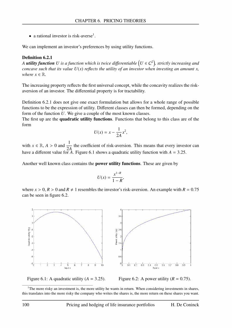
CHAPTER 6. PRICING THEORIES
• a rational investor is risk-averse1.
We can implement an investor’s preferences by using utility functions.
Definition 6.2.1A utility function U is a function which is twice differentiable
(U ∈ C2
), strictly increasing and
concave such that its value U(x) reflects the utility of an investor when investing an amount x,where x ∈ R.
The increasing property reflects the first universal concept, while the concavity realizes the risk-aversion of an investor. The differential property is for tractability.
Definition 6.2.1 does not give one exact formulation but allows for a whole range of possiblefunctions to be the expression of utility. Different classes can then be formed, depending on theform of the function U. We give a couple of the most known classes.The first up are the quadratic utility functions. Functions that belong to this class are of theform
U(x) = x −1
2Ax2,
with x ∈ R, A > 0 and1
2Athe coefficient of risk-aversion. This means that every investor can
have a different value for A. Figure 6.1 shows a quadratic utility function with A = 3.25.
Another well known class contains the power utility functions. These are given by
U(x) =x1−R
1 − R,
where x > 0, R > 0 and R , 1 resembles the investor’s risk-aversion. An example with R = 0.75can be seen in figure 6.2.
Figure 6.1: A quadratic utility (A = 3.25). Figure 6.2: A power utility (R = 0.75).
1The more risky an investment is, the more utility he wants in return. When considering investments in shares,this translates into the more risky the company who writes the shares is, the more return on these shares you want.
100 Pricing and hedging of life insurance portfolios H. De Coninck
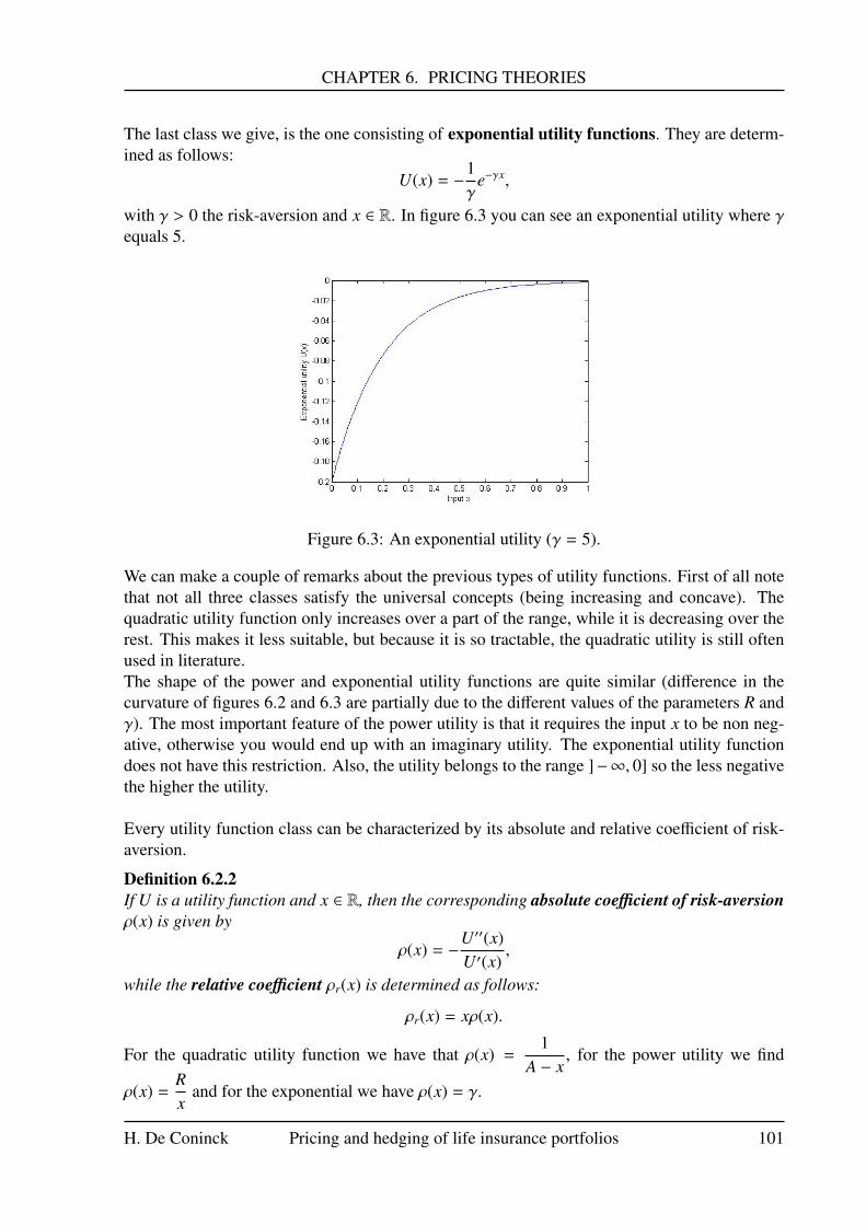
CHAPTER 6. PRICING THEORIES
The last class we give, is the one consisting of exponential utility functions. They are determ-ined as follows:
U(x) = −1γ
e−γx,
with γ > 0 the risk-aversion and x ∈ R. In figure 6.3 you can see an exponential utility where γequals 5.
Figure 6.3: An exponential utility (γ = 5).
We can make a couple of remarks about the previous types of utility functions. First of all notethat not all three classes satisfy the universal concepts (being increasing and concave). Thequadratic utility function only increases over a part of the range, while it is decreasing over therest. This makes it less suitable, but because it is so tractable, the quadratic utility is still oftenused in literature.The shape of the power and exponential utility functions are quite similar (difference in thecurvature of figures 6.2 and 6.3 are partially due to the different values of the parameters R andγ). The most important feature of the power utility is that it requires the input x to be non neg-ative, otherwise you would end up with an imaginary utility. The exponential utility functiondoes not have this restriction. Also, the utility belongs to the range ]−∞, 0] so the less negativethe higher the utility.
Every utility function class can be characterized by its absolute and relative coefficient of risk-aversion.
Definition 6.2.2If U is a utility function and x ∈ R, then the corresponding absolute coefficient of risk-aversionρ(x) is given by
ρ(x) = −U′′(x)U′(x)
,
while the relative coefficient ρr(x) is determined as follows:
ρr(x) = xρ(x).
For the quadratic utility function we have that ρ(x) =1
A − x, for the power utility we find
ρ(x) =Rx
and for the exponential we have ρ(x) = γ.
H. De Coninck Pricing and hedging of life insurance portfolios 101

CHAPTER 6. PRICING THEORIES
This shows that the exponential utility function has a constant absolute coefficient of risk-aversion, namely the risk-aversion itself.
As said before, the price is determined by demanding that it makes the choice of investingor not investing indifferent. This is done by setting the value of not investing equal to the max-imum of the expected utility function in case of investment.More mathematically, if w is the initial wealth of an investor, V(w) is the value of his wealthat time T without making any risky investments and w(T ) is the wealth an investor can receiveby investing in risk (taking into account he will have to pay a price for investing), then theindifference price of this investment is determined by the following equation:
V(w) = supw(T )E[U(w(T ))] . (6.1)
102 Pricing and hedging of life insurance portfolios H. De Coninck
Chapter 7
A mortality intensity model
7.1 The settingWe based this chapter on the paper of Hainaut and Devolder (2008). The idea is to first deriveall characteristics of the process of the mortality intensity, which will be introduced later on.
We consider n insured lives with age x. The remaining lifetimes are denoted by T1, . . . ,Tn,which are random variables. We assume that they are identically distributed. Consider againthe space (Ω,F ,P) and let Hi be the smallest σ-algebras in F such that Ti is a stopping time,for i ∈ 1, . . . , n.
We also define a counting process N(t)t∈[0,T ] =
n∑i=1
ITi ≤ t
t∈[0,T ]
. This process is Markov and
counts the number of deaths that have occurred until time t. The number of deaths dependson the mortality rate µ(t, x)t∈[0,T ]. We assume that the mortality rate is positive and that thereexists a σ-algebra G ⊆ F such that µ(t, x)t∈[0,T ] is G-predictable. Last, we also assume that∫ t
0µ(s, x)ds < +∞ almost surely. We then have that F = H1 ∨ · · · ∨ Hn ∨ G.
The conditional probability of the ith insured, surviving till time t, is denoted by
PTi > t|G(T ) = exp−
∫ t
0µ(s, x)ds
.
Let λ(t)t∈[0,T ] be the compensator of the counting process N(t)t∈[0,T ]. We will also refer toλ(t)t∈[0,T ] as the stochastic mortality intensity process. Just as in chapter 5, section 5.1 weassume that there exists a kernel intensity νN(t, dy)t∈[0,T ] such that
λ(t) =
∫ +∞
0νN(t, dy).
We also let λ satisfy the following equality:
λ(t)dt = E[dN(t)|F (t)] = (n − N(t−))µ(t, x)dt. (7.1)
Note that this is still along the same line as in chapter 5, section 5.1, as well as being similarto the stochastic intensity defined in section 4.1, equations (4.16) and (4.17), so both processesshould satisfy the same properties. Two of the more important ones concern the martingale
103
CHAPTER 7. A MORTALITY INTENSITY MODEL
property and the alternative expression for the expected number of survivors conditional on F .We give them below.Since λ(t)t∈[0,T ] is defined as the compensator of N(t)t∈[0,T ] we know that M(t)t∈[0,T ] = (N −λ)(t)t∈[0,T ] is a P-martingale. See the resemblance with equations (4.18) and (4.19).Consider s < t, the expected number of survivors at time t given F (s) is defined by E[(n −N(t))|F (s)]. Whether or or not an insured survives, depends on the insureds that are still aliveat time s (which you know since F (s) is given) and the mortality trend on [s, t]. The last isdetermined by µ(t, x)t∈[0,T ] so we find
E[(n − N(t))|F (s)] = E[E [(n − N(t))|F (s) ∨ G(T )]
∣∣∣F (s)]
by tower property
=
[(n − N(s))︸ ︷︷ ︸F (s)-measurable
exp−
∫ t
sµ(y, x)dy
∣∣∣∣∣∣F (s)]
= (n − N(s))E[exp
−
∫ t
sµ(y, x)dy
∣∣∣∣∣∣F (s)]
= (n − N(s))E[exp
−
∫ t
sµ(y, x)dy
∣∣∣∣∣∣G(s)]. µ(t, x)t∈[0,T ] depends on G
This is in analogy with the similar expression found in the proof of Proposition 4.2.1 (see thecalculation of B). We now assume that there exists a deterministic function µ(t, x)t∈[0,T ] and apredictable process X(t)t∈[0,T ] (since µ is predictable), solely dependent on G, that has mean-reverting dynamics
dX(t) = δ(β − X(t))dt + σdL(t), (7.2)
where δ, β and σ are constants and L(t)t∈[0,T ] is a Levy process, such that
µ(x, t) = µ(x, t) + X(t). (7.3)
We then have
E[(n − N(t))|F (s)] = (n − N(s))E[exp
−
∫ t
sµ(y, x)dy
∣∣∣∣∣∣G(s)]
= (n − N(s))E[exp
−
∫ t
s(µ(y, x) + X(y))dy
∣∣∣∣∣∣G(s)]
by equation (7.3)
= (n − N(s))E[exp
−
∫ t
sµ(y, x)dy
exp
−
∫ t
sX(y)dy
∣∣∣∣∣∣G(s)]
= (n − N(s)) exp−
∫ t
sµ(y, x)dy
E
[exp
−
∫ t
sX(y)dy
∣∣∣∣∣∣G(s)].
since µ(y, x) deterministic
Consider the first integral and let x ≡ x + s, then we have that the integral goes from s − s = 0till t − s:
E[(n − N(t))|F (s)] = (n − N(s)) exp−
∫ t−s
0µ(y, x + s)dy
︸ ︷︷ ︸
t−spx+s
E[exp
−
∫ t
sX(y)dy
∣∣∣∣∣∣G(s)]
104 Pricing and hedging of life insurance portfolios H. De Coninck
CHAPTER 7. A MORTALITY INTENSITY MODEL
= (n − N(s))t−spx+sE[exp
−
∫ t
sX(y)dy
∣∣∣∣∣∣G(s)]. (7.4)
Remember equation (4.45) from chapter 4, section 4.3. In this case we have the probability thata person of starting age x, at time s survives till time t.
Since µ(t, x)t∈[0,T ] is a mortality rate, it makes sense that it is increasing. Thus L(t)t∈[0,T ] shouldalso be increasing therefore we take L(t)t∈[0,T ] a subordinator. From Proposition 2.0.10 we knowthat in particular the variance σ (remember the definition of a subordinator, Definition 2.0.24,which says that it is a one-dimensional process) equals zero. From Proposition 2.0.11 we knowthat the Levy-Ito decomposition and the Levy-Khintchine representation are given by Theorem2.0.6.Besides taking L(t)t∈[0,T ] a subordinator, we also assume that there is no drift (b = 0) in thissetting. We then find
L(t) =
∫|x|<1
xJL(t, dx) +
∫|x|≥1
xJL(t, dx) by Theorem 2.0.6 and the previous assumptions
=
∫ +∞
−∞
xJL(t, dx). (7.5)
Here JL is the Poisson random measure for X(t)t∈[0,T ] and we denote the compensator of JL as νL.From Proposition 2.0.8 we know that (JL− tνL) is a martingale-valued measure. This, combined
with equation (7.5), tells us that t∫ +∞
−∞
xνL(dx) is the compensator of L(t)t∈[0,T ].
In the next part of this section we will derive a couple of properties for the process X(t)t∈[0,T ],which we introduced in equation (7.3). Before doing so, we first derive the solutions to theformer integrals, since they will be often needed. For s ≤ t we have∫ t
seδxdx =
eδt − eδs
δ(7.6)
and ∫ t
se−δ(t−x)dx =
1δ
∫ 0
−δ(t−s)eudu =
1 − e−δ(t−s)
δ. (7.7)
We start by proving an alternative expression for X(t)t∈[0,T ].
Lemma 7.1.1Take s and t in [0,T], with s < t. Then we have that
X(t) =(1 − e−δ(t−s)
)β + e−δ(t−s)X(s) + σ
∫ t
se−δ(t−x)dL(x)
is a solution to the stochastic differential equation (7.2).
Proof. Consider f (t, X(t)) = eδtX(t). We can then make use of the integrating factor and equa-tion (7.2) to arrive at
d f (t, X(t)) = d(eδtX(t)
)= eδt(dX(t) + δX(t)dt) = eδt(δβdt + σdL(t)).
H. De Coninck Pricing and hedging of life insurance portfolios 105

CHAPTER 7. A MORTALITY INTENSITY MODEL
Integrating the latter over the interval [s, t] and applying the equality (7.6) we obtain
eδtX(t) − eδsX(s) = β(eδt − eδs
)+ σ
∫ t
seδxdL(x)
⇔ X(t) = β(1 − eδ(s−t)
)+ eδ(s−t)X(s) + σ
∫ t
seδ(x−t)dL(x)
⇔ X(t) = β(1 − e−δ(t−s)
)+ e−δ(t−s)X(s) + σ
∫ t
se−δ(t−x)dL(x).
We can now use Lemma 7.1.1 to calculate the conditional characteristic function of X(t)t∈[0,T ],which is analogue to Definition 2.0.18. For s < t, we get
φX(t)(iu|F (s)) = E[expiuX(t)|F (s)
]= E
[exp
iu
( (1 − e−δ(t−s)
)β + e−δ(t−s)X(s)︸ ︷︷ ︸
F (s)-measurable
+σ
∫ t
se−δ(t−x)dL(x)
)∣∣∣∣∣∣F (s)]
= expiu
(β(1 − e−δ(t−s)
)+ e−δ(t−s)X(s)
)E
[exp
iuσ
∫ t
se−δ(t−x)dL(x)
∣∣∣∣∣∣F (s)].
(7.8)
We can do the same for∫ t
sX(y)dy. We replace X(y) with the expression proven in Lemma 7.1.1
and keep in mind equation (7.7), before calculating the conditional characteristic function.∫ t
sX(y)dy =
∫ t
s
((1 − e−δ(y−s)
)β + e−δ(y−s)X(s) + σ
∫ y
se−δ(y−x)dL(x)
)dy
= β(t − s) − β∫ t
se−δ(y−s)dy + X(s)
∫ t
se−δ(y−s)dy + σ
∫ t
s
∫ y
se−δ(y−x)dL(x)dy
= β(t − s) − β∫ t
se−δ(y−s)dy + X(s)
∫ t
se−δ(y−s)dy + σ
∫ t
s
∫ t
xe−δ(y−x)dydL(x)
by Theorem 2.0.7
= β(t − s) +(1 − e−δ(t−s)
) X(s) − βδ
+σ
δ
∫ t
s
(1 − e−δ(t−x)
)dL(x). (7.9)
The conditional characteristic function, with s < t, is then found as follows:
φ∫ ts X(y)dy(iu|F (s))
= E[exp
iu
∫ t
sX(y)dy
∣∣∣∣∣∣F (s)]
= E[
exp
iu(β(t − s) +
(1 − e−δ(t−s)
) (X(s) − β)δ︸ ︷︷ ︸
F (s)-measurable
+σ
δ
∫ t
s
(1 − e−δ(t−x)
)dL(x)
)∣∣∣∣∣∣F (s)]
by equation (7.9)
106 Pricing and hedging of life insurance portfolios H. De Coninck
CHAPTER 7. A MORTALITY INTENSITY MODEL
= exp
iu(β(t − s) +
(1 − e−δ(t−s)
) (X(s) − β)δ
)E
[exp
iuσδ
∫ t
s
(1 − e−δ(t−x)
)dL(x)
∣∣∣∣∣∣F (s)].
(7.10)
Proposition 7.1.1Let L(t)t∈[0,T ] be a subordinator and k the corresponding cumulant transform. Consider acomplex-valued, left-continuous function f : [0,+∞[→ C such that there is a number M > 0for which |Re( f )| ≤ M, then, for ξ ∈ R, we have
E[exp
∫ t
0f (x)dL(ξx)
]= exp
∫ t
0ξk( f (x))dx
.
As said in chapter 2, you can consider different classes within the Levy processes and in partic-ular we will have a look at the class of α-stable subordinators.
Definition 7.1.1A subordinator L(t)t∈[0,T ] is called an α-stable subordinator, with α ∈ [0, 1[ if for all a > 0 and
all t ∈ [0,T ] you have thatL(at)
a1α
equals L(t) in distribution.
One of the advantages of the α-stable subordinator is that it has a relatively easy Levy measureto work with:
νL(x) =c
xα+1 Ix > 0,
where c is a positive constant.
Instead of working with the original Levy measure, you can choose to transform it. As longas you use a transformation that respects the integrability conditions, the new measure is againa Levy measure. For the measure of the α-stable subordinator, the tempered one is found bymultiplying it with a decreasing exponential function. Here we will use the following exponen-tial: e−ωx, with ω a positive constant. We then find the tempered Levy measure for the α-stablesubordinator:
νL(x) =ce−ωx
xα+1 Ix > 0. (7.11)
We now want to derive a formula for the cumulant transform of L(t)t∈[0,T ], remember Defini-tion 2.0.19. Since in chapter 2 we showed the relation between the mgf and the characteristicfunction, we can find, for u ∈ R, that
φL(t)(u) = φL(t)(i(−iu))
= exp
t∫R
(ei(−iu)x − 1
)νL(dx)
by Theorem 2.0.6 with b = 0
= exp
t∫ +∞
0(eux − 1) νL(dx)
. νL is non zero on [0,+∞[ (7.12)
So now we have that the cumulant transform is given by
k(u) = ln φL(1)(u)
H. De Coninck Pricing and hedging of life insurance portfolios 107

CHAPTER 7. A MORTALITY INTENSITY MODEL
=
∫ +∞
0(eux − 1) νL(dx) by equation (7.12) (7.13)
=
∫ +∞
0(eux − 1)
ce−ωx
xα+1 dx by equation 7.11
= c∫ +∞
0
e−(ω−u)x
xα+1 dx − c∫ +∞
0
e−ωx
xα+1 dx.
We consider two cases: α , 0 and α = 0. Take α , 0. In the first integral let z = (ω − u)x, or
thus x =z
ω − uand dx =
dzω − u
. For the second integral we take z = ωx such that x =zω
and
dx =dzω
. Note that in both substitutions the integrand boundaries do not change. We obtain
k(u) = c∫ +∞
0e−z
( zω − u
)−α−1 dzω − u
− c∫ +∞
0e−z
( zω
)−α−1 dzω
=c
ω − u(ω − u)α+1
∫ +∞
0e−zz−α−1dz︸ ︷︷ ︸Γ(−α)
−cωωα+1
∫ +∞
0e−zz−α−1dz︸ ︷︷ ︸Γ(−α)
= cΓ(−α) ((ω − u)α − ωα) . (7.14)
For α = 0 we don’t split up the integral. Instead we rewrite it so we can make use of thefollowing series expansion:
eux − 1x
=1x
+∞∑n=0
(ux)n
n!− 1
=
+∞∑n=1
unxn−1
n!. (7.15)
We then find, for positive u,
k(u) = c∫ +∞
0e−ωx eux − 1
xdx
= c∫ +∞
0e−ωx
+∞∑n=1
unxn−1
n!dx by equation (7.15)
= c+∞∑n=1
un
n!
∫ +∞
0e−ωxxn−1dx︸ ︷︷ ︸
e−ωx ∑n−1k=0
(−1)n−1−k (n−1)!xk
k!(−ω)n−k
see remark following Theorem 2.0.7
= ce−ωx+∞∑n=1
un
n
n−1∑k=0
(−1)n−1−kxk
k!(−ω)n−k
∣∣∣∣∣∣+∞0
.
Note that e−ωx is the inverse of eωx, so therefore e−ωx must drop as fast as eωx grows. It isgeneraly known that the exponential eωx grows faster than the polynomial xk and this for allk ∈ N. Consequently e−ωx approaches zero faster than xk approaches infinity. For this we reasonwe see that the only term that remains in the second summation, is the one in the lowerboundx = 0 for k = 0:
k(u) = −c+∞∑n=1
(−1)n−1(−uω
)n
n
108 Pricing and hedging of life insurance portfolios H. De Coninck

CHAPTER 7. A MORTALITY INTENSITY MODEL
= −c ln(1 −
uω
), (7.16)
where the last equality only holds if −1 <uω< 1.
Apply Proposition 7.1.1 to equation (7.8), with f (x) = iuσe−δ(t−x) and ξ = 1. This gives us
φX(t)(iu|F (s)) = expiu
(β(1 − e−δ(t−s)
)+ e−δ(t−s)X(s)
)exp
∫ t
sk(iuσe−δ(t−x)
)dx
.
Assume that α , 0. We can then make use of equation (7.14) in the previous equation and find
φX(t)(iu|F (s))
= expiu
(β(1 − e−δ(t−s)
)+ e−δ(t−s)X(s)
)exp
∫ t
scΓ(−α)
((ω − iuσe−δ(t−x)
)α− ωα
)dx
,
(7.17)
while for α = 0 we use equation (7.16) to obtain
φX(t)(iu|F (s)) = expiu
(β(1 − e−δ(t−s)
)+ e−δ(t−s)X(s)
)exp
∫ t
s−c ln
(1 −
iuσe−δ(t−x)
ω
)dx
.
(7.18)
The previous derived expressions can be used to calculate the first and second moment (seechapter 2), which ultimately will give us the mean and variance. For α , 0 we use equation(7.17). Since φX(t)(iu|F (t)) takes on an exponential form we find
E [X(t)|F (s)]
=1i∂
∂uφX(t)(iu|F (s))
∣∣∣∣∣u=0
=1iφX(t)(iu|F (s))
×
(i(β(1 − e−δ(t−s)
)+ e−δ(t−s)X(s)
)−
∫ t
sicΓ(−α)α
(ω − iuσe−δ(t−y)
)α−1σe−δ(t−y)dy
) ∣∣∣∣∣∣u=0
= β(1 − e−δ(t−s)
)+ e−δ(t−s)X(s) − cασωα−1Γ(−α)
∫ t
se−δ(t−x)dx
= β(1 − e−δ(t−s)
)+ e−δ(t−s)X(s) − cΓ(−α)αωα−1σ
δ
(1 − e−δ(t−s)
).
by equation (7.7) (7.19)
If on the other hand α = 0, we get from equation (7.18) and (7.7)
E [X(t)|F (s)]
=1i∂
∂uφX(t)(iu|F (s))
∣∣∣∣∣u=0
=1iφX(t)(iu|F (t))
×
i (β (1 − e−δ(t−s)
)+ e−δ(t−s)X(s)
)+ c
∫ t
s
1
1 − iuσe−δ(t−y)
ω
iσe−δ(t−y)
ωdy
∣∣∣∣∣∣u=0
H. De Coninck Pricing and hedging of life insurance portfolios 109
CHAPTER 7. A MORTALITY INTENSITY MODEL
= β(1 − e−δ(t−s)
)+ e−δ(t−s)X(s) +
cωσ
∫ t
se−δ(t−x)dx
= β(1 − e−δ(t−s)
)+ e−δ(t−s)X(s) +
cω
σ
δ
(1 − e−δ(t−s)
). (7.20)
In order to find an expression for the variance in both cases, we first need to calculate the secondmoment. For α , 0, making use of the previous calculations, we find
E[X2(t)|F (s)
]=
1i2
∂2
∂u2φX(t)(iu|F (s))∣∣∣∣∣u=0
= −∂
∂u
[φX(t)(iu|F (s))
×
(i(β(1 − e−δ(t−s)
)+ e−δ(t−s)X(s)
)−
∫ t
sicΓ(−α)α
(ω − iuσe−δ(t−x)
)α−1σe−δ(t−x)dx
) ]∣∣∣∣∣∣u=0
=
[−∂
∂uφX(t)(iu|F (s))
×
(i(β(1 − e−δ(t−s)
)+ e−δ(t−s)X(s)
)−
∫ t
sicΓ(−α)α
(ω − iuσe−δ(t−x)
)α−1σe−δ(t−x)dx
)− φX(t)(iu|F (s))
×∂
∂u
(i(β(1 − e−δ(t−s)
)+ e−δ(t−s)X(s)
)−
∫ t
sicΓ(−α)α
(ω − iuσe−δ(t−x)
)α−1σe−δ(t−x)dx
) ]∣∣∣∣∣∣u=0
=
[− φX(t)(iu|F (s))
×
(i(β(1 − e−δ(t−s)
)+ e−δ(t−s)X(s)
)−
∫ t
sicΓ(−α)α
(ω − iuσe−δ(t−x)
)α−1σe−δ(t−x)dx
)2
+ φX(t)(iu|F (s))∫ t
scΓ(−α)α(α − 1)
(ω − iuσe−δ(t−x)
)α−2σ2e−2δ(t−x)dx
]∣∣∣∣∣∣u=0
=
((β(1 − e−δ(t−s)
)+ e−δ(t−s)X(s)
)− cΓ(−α)αωα−1σ
δ
(1 − e−δ(t−s)
))2
+ cΓ(−α)α(α − 1)ωα−2σ2∫ t
se−2δ(t−x)dx
=
((β(1 − e−δ(t−s)
)+ e−δ(t−s)X(s)
)− cΓ(−α)αωα−1σ
δ
(1 − e−δ(t−s)
))2
+ cΓ(−α)α(α − 1)ωα−2σ2
2δ
(1 − e−2δ(t−s)
).
by equation (7.7) with 2δ instead of δ (7.21)
Noting that the first term after the equality equals the squared expectation and recalling equation(7.19) we arrive at
E[X2(t)|F (s)
]= E2 [X(t)|F (s)] + cΓ(−α)α(α − 1)ωα−2σ
2
2δ
(1 − e−2δ(t−s)
)⇔ E
[X2(t)|F (s)
]− E2 [X(t)|F (s)] = cΓ(−α)α(α − 1)ωα−2σ
2
2δ
(1 − e−2δ(t−s)
)110 Pricing and hedging of life insurance portfolios H. De Coninck

CHAPTER 7. A MORTALITY INTENSITY MODEL
var(X(t)|F (s)) = cΓ(−α)α(α − 1)ωα−2σ2
2δ
(1 − e−2δ(t−s)
), (7.22)
while for α = 0 we get in an analogous way, recalling equation (7.19),
E[X2(t)|F (s)
]=
1i2
∂2
∂u2φX(t)(iu|F (s))|u=0
= −∂
∂u
[φX(t)(iu|F (s))
i (β (1 − e−δ(t−s)
)+ e−δ(t−s)X(s)
)+ c
∫ t
s
1
1 − iuσe−δ(t−x)
ω
iσe−δ(t−x)
ωdx
]∣∣∣∣∣∣u=0
=
[−∂
∂uφX(t)(iu|F (s))
i (β (1 − e−δ(t−s)
)+ e−δ(t−s)X(s)
)+ c
∫ t
s
1
1 − iuσe−δ(t−x)
ω
iσe−δ(t−x)
ωdx
− φX(t)(iu|F (s))
∂
∂u
i (β (1 − e−δ(t−s)
)+ e−δ(t−s)X(s)
)+ c
∫ t
s
1
1 − iuσe−δ(t−x)
ω
iσe−δ(t−x)
ωdx
]∣∣∣∣∣∣u=0
=
[− φX(t)(iu|F (s))
i (β (1 − e−δ(t−s)
)+ e−δ(t−s)X(s)
)+ c
∫ t
s
1
1 − iuσe−δ(t−x)
ω
iσe−δ(t−x)
ωdx
2
− φX(t)(iu|F (s))c∫ t
s
1(1 − iuσe−δ(t−x)
ω
)2
iσe−δ(t−x)
ω
iσe−δ(t−x)
ωdx
]∣∣∣∣∣∣u=0
=
((β(1 − e−δ(t−s)
)+ e−δ(t−s)X(s)
)+
cω
σ
δ
(1 − e−δ(t−s)
))2+
cω2σ
2∫ t
se−2δ(t−x)dx
=
((β(1 − e−δ(t−s)
)+ e−δ(t−s)X(s)
)+
cω
σ
δ
(1 − e−δ(t−s)
))2+
cω2
σ2
2δ
(1 − e−2δ(t−s)
).
by equation (7.7) with 2δ instead of δ
And thus we obtain
E[X2(t)|F (s)
]= E2 [X(t)|F (s)] +
cω2
σ2
2δ
(1 − e−2δ(t−s)
)⇔ E
[X2(t)|F (s)
]− E2 [X(t)|F (s)] =
cω2
σ2
2δ
(1 − e−2δ(t−s)
)var(X(t)|F (s)) =
cω2
σ2
2δ
(1 − e−2δ(t−s)
). (7.23)
The calculated expectations and variances can then be used to derive the long term behaviour ofthe process X(t)t∈[0,T ]. We do this by taking the limit for t going to +∞. When α , 0, we havethe following equation for the expectation:
limt→+∞
E[X(t)|F (s)] = limt→+∞
[β(1 − e−δ(t−s)
)+ e−δ(t−s)X(s) − cΓ(−α)αωα−1σ
δ
(1 − e−δ(t−s)
)]by equation (7.19)
= β − cΓ(−α)αωα−1σ
δ, (7.24)
while for α = 0 we get
limt→+∞
E[X(t)|F (s)] = limt→+∞
[β(1 − e−δ(t−s)
)+ e−δ(t−s)X(s) +
cω
σ
δ
(1 − e−δ(t−s)
)]by equation (7.20)
H. De Coninck Pricing and hedging of life insurance portfolios 111
CHAPTER 7. A MORTALITY INTENSITY MODEL
= β +cω
σ
δ. (7.25)
For the variance, when α , 0, we find
limt→+∞
var(X(t)|F (s)) = limt→+∞
[cΓ(−α)α(α − 1)ωα−2σ
2
2δ
(1 − e−2δ(t−s)
)]by equation (7.22)
= cΓ(−α)α(α − 1)ωα−2σ2
2δ. (7.26)
For α = 0 we have
limt→+∞
var(X(t)|F (s)) = limt→+∞
[cω2
σ2
2δ
(1 − e−2δ(t−s)
)]by equation (7.23)
=cω2
σ2
2δ. (7.27)
Note that all derivations are based on equation (7.8) for X(t)t∈[0,T ]. We could do the same usingequation (7.9), but as it turns out, the moments cannot be calculated analytically because theydepend on the Levy process L(t)t∈[0,T ]. We just give the final formulation without writing downall the steps, because we will need this expression later on.For certain processes, such as the Gamma process or the Inversian Gaussian process explicitformulas can be found. See for example Applebaum (2004) or Cont and Tankov (2004) formore information.
E[exp
−
∫ T
tX(s)ds
∣∣∣∣∣∣F (t)]
= exp−
(β(T − t) +
X(t) − βδ
(1 − e−δ(T−t)
))exp
∫ T
tk(−σ
δ
(1 − e−δ(T−s)
))ds
. (7.28)
7.2 The longevity risk price through the pricing measureWe assume that there is a pricing measure Q. Since we work with Levy measures we can useTheorems 6.1.1 and 6.1.3 to derive the Radon-Nikodym derivative and more specifically, theRadon-Nikodym derivative process:
Z(t) = E[dQdP
∣∣∣∣∣∣F (t)]
= eU(t). (7.29)
From Theorem 6.1.2 and Theorem 6.1.3 we also have that there exists an x ∈ R such that
θ(x) = ln
dνQLdνL
= ln
d(
ce−ωQ x
xα+1 Ix > 0)
dνL
by equation (7.11)
= ln
d(
ce(ω−ωQ)xe−ωx
xα+1 Ix > 0)
dνL
112 Pricing and hedging of life insurance portfolios H. De Coninck

CHAPTER 7. A MORTALITY INTENSITY MODEL
= ln
d(νLe(ω−ωQ)x
)dνL
by equation (7.11)
=(ω − ωQ
)x. (7.30)
Therefore, using Theorem 6.1.3 and the previous findings, we can obtain the formula for U.
U(t)
= y(L − LνL)(t) −12
ytrΣyt − γtryt + limε−→>
0
∑(s,∆L(s))∈]0,t]×|x|>ε
θ(∆L(s)) − t∫|x|>ε
(eθ(x) − 1
)νL(dx)
= lim
ε−→>
0
∑(s,∆L(s))∈]0,t]×|x|>ε
θ(∆L(s)) − t∫|x|>ε
(eθ(x) − 1
)νL(dx)
since Σ = 0 = γ, y = 0
= limε−→>
0
∑(s,∆L(s))∈]0,t]×|x|>ε
(ω − ωQ
)∆L(s) − t
∫|x|>ε
(e(ω−ωQ)x − 1
)νL(dx)
by equation (7.30)
=(ω − ωQ
)limε−→>
0
∑(s,∆L(s))∈]0,t]×|x|>ε
∆L(s) − t limε−→>
0
∫|x|>ε
(e(ω−ωQ)x − 1
)νL(dx)
=(ω − ωQ
)L(t) − t
∫|x|>0
(e(ω−ωQ)x − 1
)νL(dx). (7.31)
Implementing equation (7.31) in formula (7.29) gives us
Z(t) = eU(t) = exp(ω − ωQ
)L(t) − t
∫|x|>0
(e(ω−ωQ)x − 1
)νL(dx)
= exp
(ω − ωQ
)L(t) − t
∫ +∞
0
(e(ω−ωQ)x − 1
)νL(dx)
. (7.32)
Recall from section 7.1 the derivation of formula (7.4), which is the expected number of sur-vivors given all information until time t. We can repeat that reasoning but under the measure Qinstead of P.
EQ [(n − N(t))|F (t)] = (n − N(s))EQ[exp
−
∫ t
sµ(y, x)dy
∣∣∣∣∣∣G(s)]
= (n − N(s)) exp∫ t
sµ(y, x)dy
︸ ︷︷ ︸
t−spx+s
EQ[exp
−
∫ t
sX(y)dy
∣∣∣∣∣∣G(s)]
by equation (7.3)
= (n − N(s))t−spx+sEQ
[exp
−
∫ t
sX(y)dy
∣∣∣∣∣∣G(s)]. (7.33)
How can we now use the equivalent martingale measure Q for pricing?
Let r be the constant interest rate. Consider an insurance policy where you agree to pay anamount K at time T if the insured is still alive at this time. Assume the insured is alive attime t (when he has an age of x + t), then the price of the insurance contract at time t depends
H. De Coninck Pricing and hedging of life insurance portfolios 113
CHAPTER 7. A MORTALITY INTENSITY MODEL
on the capital K, the time of payout T , the interest rate r which we use for discounting, andthe probability of the insured surviving till the time of delivery T . More precisely we needto discount the payoff K from T till time t using the discount rate r. We also need to takeinto account the probability of the insured being alive. Equation (7.33) gives the expressionfor a group of n insureds at start time zero, so for one individual the survival probability is
just t−spx+sEQ
[exp
−
∫ t
sX(y)dy
∣∣∣∣∣∣G(s)]. Therefore we have that the price P of the insurance
contract is given by
P = Ke−r(T−t)T−t px+tE
Q
[exp
−
∫ T
tX(y)dy
∣∣∣∣∣∣G(t)].
7.3 The longevity risk price through indifference pricingAssume that an investor, which in this setting is just an insurer, has a wealth w(t) at time t. Wewill work out this part by applying an exponential utility function:
U(w(t)) = −1γ
e−γw(t). (7.34)
Remember that for this type of utilities ρ = γ (see section 6.2). We also consider a risk freeinterest rate r. The first option the investor has at time t, is to invest his/her wealth in the moneymarket where he/she will get an interest rate equal to r. The dynamics of ones money are thusgiven by
dw(t) = rw(t)dt. (7.35)
The insurer’s wealth at time T is then given by w(T ) = w(t)er(T−t).
According to the theory in section 6.2, we need to calculate the expected utility of the investor’swealth at time T , given all information till time t.
E [U(w(T ))|F (t)] = E[−
1γ
e−γw(T )
∣∣∣∣∣∣F (t)]
by equation (7.34)
= −1γ
E[
exp−γw(t)er(T−t)
︸ ︷︷ ︸F (t)-measurable
∣∣∣∣F (t)]
= −1γ
exp−γw(t)er(T−t)
. (7.36)
The insurer also has an alternative, instead of investing in the money market he/she could acceptthe risks of a number of n insureds. At time T one then has to pay an amount H(X,N), dependenton how many of the insureds are still alive and on the process X(t)t∈[0,T ]. In return the insurerreceives a total premium P, which is the sum of all the individual premiums each insured haspaid. Therefore the initial wealth at time t equals w(t) + P, instead of w(t), while the expectedwealth at time T given F (t) is as follows:
E[U(w(T ) − H(X(T ),N(T )))|F (t)] = E[−
1γ
e−γ(w(T )−H(X(T ),N(T )))
∣∣∣∣∣∣F (t)]
by equation (7.34)
114 Pricing and hedging of life insurance portfolios H. De Coninck

CHAPTER 7. A MORTALITY INTENSITY MODEL
= −1γ
E[exp
−γ
((w(t) + P)er(T−t) − H(X(T ),N(T ))
) ∣∣∣∣F (t)]
= −1γ
E[
exp−γ
((w(t) + P)er(T−t)
)︸ ︷︷ ︸F (t)-measurable
eγH(X(T ),N(T ))∣∣∣∣F (t)
]= −
1γ
exp−γ
((w(t) + P)er(T−t)
)E
[eγH(X(T ),N(T ))
∣∣∣F (t)].
(7.37)
While in the first case the expected utility is relatively easy to calculate, for the alternative thisis not always the case. In order to resolve this, you can try to build a partial differential equationthat has E[U(w(T ) − H(X(T ),N(T )))|F (t)] as a solution.
Proposition 7.3.1Assume that V(t,w(t) + P, X(t),N(t))t∈[0,T ] is sufficiently differentiable and that all necessaryintegrability conditions are fulfilled. We then have that V(t,w(t) + P, X(t),N(t)) = E[U(w(T ) −H(X(T ),N(T )))|F (t)] is a solution of
∂V∂t
+ r(w(t) + P)∂V∂wP
+ δ(β − X(t))∂V∂x
+
∫ +∞
0(V(t,w(t) + P, X(t−) + σy,N(t−)) − V(t,w(t) + P, X(t−),N(t−))) νL(dy)
+ (V(t,w(t) + P, X(t−),N(t−) + 1) − V(t,w(t) + P, X(t−),N(t−))) (n − N(t−))µ(t, x) = 0,
where V(t,w(t) + P, X(t),N(t))t∈[0,T ] can be seen as a function V in the variables t, wP, x and nwhich we evaluate at the point (t,w(t) + P, X(t),N(t)).
Proof. By equation (7.37) and the fact that N is a Markov process (see section 6.2) we have that
V(t,w(t) + P, X(t),N(t)) = E[U(w(T ) − H(X(T ),N(T )))|F (t)]
= −1γ
exp−γ(w(t) + P)er(T−t)
E
[eγH(X(T ),N(T ))
∣∣∣F (t)]
⇔ expγ(w(t) + P)er(T−t)
V(t,w(t) + P, X(t),N(t)) = −
1γ
E[eγH(X(T ),N(T ))
∣∣∣F (t)].
Since, for s < t, we have that
E[exp
γ(w(t) + P)er(T−t)
V(t,w(t) + P, X(t),N(t))
∣∣∣∣F (s)]
= −1γ
E[E
[eγH(X(T ),N(T ))
∣∣∣F (t)] ∣∣∣∣F (s)
]= −
1γ
E[eγH(X(T ),N(T ))
∣∣∣F (s)]
= expγ(w(s) + P)er(T−s)
V(s,w(s) + P, X(s),N(s)) (7.38)
so(exp
γ(w(t) + P)er(T−t)
V(t,w(t) + P, X(t),N(t))
)t∈[0,T ]
is a P-martingale. Note that implicitlywe have assumed that H(X(T ),N(T )) is independent of t. Therefore using Ito’s formula, weshould have a dt-term equal to zero.
d(exp
γ(w(t) + P)er(T−t)
V(t,w(t) + P, X(t),N(t))
)H. De Coninck Pricing and hedging of life insurance portfolios 115
CHAPTER 7. A MORTALITY INTENSITY MODEL
= expγ(w(t) + P)er(T−t)
dV(t,w(t) + P, X(t),N(t))
+ V(t,w(t) + P, X(t),N(t))d expγ(w(t) + P)er(T−t)
+ d exp
γ(w(t) + P)er(T−t)
dV(t,w(t) + P, X(t),N(t))︸ ︷︷ ︸
0 since first term contains only dt-terms
= expγ(w(t) + P)er(T−t)
dV(t,w(t) + P, X(t),N(t))
+ V(t,w(t) + P, X(t),N(t)) expγ(w(t) + P)er(T−t)
(γer(T−t)r(w(t) + P)dt − rγ(w(t) + P)er(T−t)dt
)= exp
γ(w(t) + P)er(T−t)
dV(t,w(t) + P, X(t),N(t)).
The latter shows that equating the dt-part of expγ(w(t) + P)er(T−t)
V(t,w(t) + P, X(t),N(t)) to
zero is equivalent with equating the dt-term of V(t,w(t) + P, X(t),N(t)) to zero. In order tocalculate dV(t,w(t) + P, X(t),N(t)) we want to make use of Theorem 2.0.5. We first show thatw + P, X and N are all Ito-Levy processes.
We have that w + P is an Ito-Levy process since
d(w(t) + P) = r(w(t) + P)dt,
with α(t) = r(w(t) + P) and β(t) = 0 = γ(t, y); for X we have that
dX(t) = δ(β − X(t))dt + σ
∫ +∞
0yJL(dt, dy) by equation (7.2)
=
(δ(β − X(t)) +
∫ +∞
0σyνL(dy)
)dt +
∫ +∞
0σy (JL(dt, dy) − νL(dy)dt) ,
where α(t) = δ(β − X(t)) +
∫ +∞
0σyνL(dy), β(t) = 0 and γ(t, y) = σy; and for N we have that
dN(t) =
∫ +∞
0JN(dt, dy)
=
∫ +∞
0νN(t, dy)dt +
∫ +∞
0(JN(dt, dy) − νN(t, dy)dt) .
We note that here the compensator νN(t, dy)dt of JN(dt, dy) is time-dependent and more specificwe have that νN(t, dy) = λ(t) f (dy), with λ(t)t∈[0,T ] the intensity process and f the correspondingdensity of the jump sizes (here the jump sizes equal zero or one). It then follows that
dN(t) = λ(t)∫ +∞
0f (dy)︸ ︷︷ ︸
1
dt +
∫ +∞
0(JN(dt, dy) − νN(t, dy)dt)
= λ(t)dt +
∫ +∞
0(JN(dt, dy) − νN(t, dy)dt) ,
with α(t) = λ(t), β = 0 and γ(t, y) = 1. By applying Theorem 2.0.5 we then arrive at
dV(t,w(t) + P, X(t),N(t))
116 Pricing and hedging of life insurance portfolios H. De Coninck

CHAPTER 7. A MORTALITY INTENSITY MODEL
=∂V∂t
dt + r(w(t) + P)∂V∂wP
dt + δ(β − X(t))∂V∂x
dt +
∫ +∞
0σyνL(dy)
∂V∂x
dt + λ(t)∂V∂n
dt
+
∫ +∞
0
(V(t,w(t) + P, X(t−) + σy,N(t−)) − V(t,w(t) + P, X(t−),N(t−)) − σy
∂V∂x
)νL(dy)dt
+
∫ +∞
0(V(t,w(t) + P, X(t−) + σy,N(t−)) − V(t,w(t) + P, X(t−),N(t−))) (JL(dt, dy) − νL(dy)dt)
+
∫ +∞
0
(V(t,w(t) + P, X(t−),N(t−) + 1) − V(t,w(t) + P, X(t−),N(t−)) −
∂V∂n
)νN(t, dy)dt
+
∫ +∞
0(V(t,w(t) + P, X(t−),N(t−) + 1) − V(t,w(t) + P, X(t−),N(t−))) (JN(dt, dy) − νN(t, dy)dt)
=∂V∂t
dt + r(w(t) + P)∂VwP
dt + δ(β − X(t))∂V∂x
dt
+
∫ +∞
0(V(t,w(t) + P, X(t−) + σy,N(t−)) − V(t,w(t) + P, X(t−),N(t−))) νL(dy)dt
+
∫ +∞
0(V(t,w(t) + P, X(t−) + σy,N(t−)) − V(t,w(t) + P, X(t−),N(t−))) (JL(dt, dy) − νL(dy)dt)
+ (V(t,w(t) + P, X(t−),N(t−) + 1) − V(t,w(t) + P, X(t−),N(t−))) λ(t)dt
+
∫ +∞
0(V(t,w(t) + P, X(t−),N(t−) + 1) − V(t,w(t) + P, X(t−),N(t−))) (JN(dt, dy) − νN(t, dy)dt) .
Recalling Proposition 2.0.8, we can now set the dt-part in the latter equal to zero:
∂V∂t
+ r(w(t) + P)∂V∂wP
+ δ(β − x(t))∂V∂x
+
∫ +∞
0(V(t,w(t) + P, X(t−) + σy,N(t−)) − V(t,w(t) + P, X(t−),N(t−))νL(dy)
+ (V(t,w(t) + P, X(t−),N(t−) + 1) − V(t,w(t) + P, X(t−),N(t−)))λ(t) = 0
⇔∂V∂t
+ r(w(t) + P)∂V∂wP
+ δ(β − x(t))∂V∂x
+
∫ +∞
0(V(t,w(t) + P, X(t−) + σy,N(t−)) − V(t,w(t) + P, X(t−),N(t−))νL(dy)
+ (V(t,w(t) + P, X(t−),N(t−) + 1) − V(t,w(t) + P, X(t−),N(t−)))(n − N(t−))µ(t, x) = 0.by equation (7.1)
According to section 6.2, formula (6.1), we then have that the price is found by solving
E[U(w(T ))|F (t)] = E[U(w(T ) − H(X(T ),N(T ))|F (t)]
⇔ −1γ
exp−γw(t)er(t−t)
= −
1γ
exp−γ(w(t) + P)er(T−t)
E
[eγH(X(T ),N(T ))
∣∣∣F (t)]
⇔ expγPer(T−t)
= E
[eγH(X(T ),N(T ))
∣∣∣F (t)]
⇔ P =1γ
e−r(T−t) ln(E
[eγH(X(T ),N(T ))
∣∣∣F (t)]).
H. De Coninck Pricing and hedging of life insurance portfolios 117

CHAPTER 7. A MORTALITY INTENSITY MODEL
The above equation holds in general. The idea is to derive an expression for the logarithmicpart by assuming a specific setting. Consider again an insurance contract where you have topay an amount K to an insured provided that the insured is still alive at time T , knowing he/shehas survived until time t and has reached an age x + t. The risk free rate is again r. ThenH(X(T ),N(T )) = (1 − N(T ))K, such that
E[U(w(T ) − H(X(T ),N(T ))|F (t)] = −1γ
exp−γ(w(t) + P)er(T−t)
E
[eγH(X(T ),N(T ))
]= −
1γ
exp−γ(w(t) + P)er(T−t)
E
[eγ(1−N(T ))K
∣∣∣F (t)]. (7.39)
We can also determine the insurer’s expected utility at time t, which equals V(t,w(t)+P, X(t), 0).
Proposition 7.3.2The insurer’s expected utility at time t is given by
V(t,w(t) + P, X(t), 0)
= −1γ
exp−γer(T−t)(w(t) + P)
(1 − T−t px+tE
[exp
−
∫ T
tX(s)ds
∣∣∣∣∣∣G(t)] (
1 − eγK)),
where again V can be seen as a function in the variables t, wP, x and n evaluated at (t,w(t) +
P, X(t), 0).
Proof. In order to prove the expected utility given just above, we need to show that this expres-sion is a solution of the partial differential equation determined in Proposition 7.3.1. First of all,this means calculating a couple of derivatives.
∂
(T−t px+tE
[exp
−
∫ T
tX(s)ds
∣∣∣∣∣∣G(t)])
∂t
=∂T−t px+t
∂tE
[exp
−
∫ T
tX(s)ds
∣∣∣∣∣∣G(t)]
+ T−t px+t
∂E[exp
−
∫ T
tX(s)ds
∣∣∣∣∣∣G(t)]
∂t
= T−t px+tµ(t, x)E[exp
−
∫ T
tX(s)ds
∣∣∣∣∣∣G(t)]
+ T−t px+tE[exp
−
∫ T
tX(s)ds
∣∣∣∣∣∣G(t)]
×
(β +
X(t) − βδ
e−δ(T−t)δ − k(−σ
δ
(1 − e−δ(T−t)
)))by equations (7.4) and (7.28), using the chain rule
= T−t px+tE[exp
−
∫ T
tX(s)ds
∣∣∣∣∣∣G(t)] (β + (X(t) − β)e−δ(T−t) − k
(−σ
δ
(1 − e−δ(T−t)
))+ µ(t, x)
),
(7.40)
∂
(T−t px+tE
[exp
−
∫ T
tX(s)ds
∣∣∣∣∣∣G(t)])
∂x
118 Pricing and hedging of life insurance portfolios H. De Coninck

CHAPTER 7. A MORTALITY INTENSITY MODEL
=∂T−t px+t
∂xE
[exp
−
∫ T
tX(s)ds
∣∣∣∣∣∣G(t)]
+ T−t px+t
∂E[exp
−
∫ T
tX(s)ds
∣∣∣∣∣∣G(t)]
∂x
= 0 − T−t px+tE[exp
−
∫ T
tX(s)ds
∣∣∣∣∣∣G(t)]
1δ
(1 − e−δ(T−t)
)by equations (7.4) and (7.28), using the chain rule
= −T−t px+tE[exp
−
∫ T
tX(s)ds
∣∣∣∣∣∣G(t)]
1 − e−δ(T−t)
δ.
(7.41)
Equation (7.40) and equation (7.41) can now be used to calculate the derivatives of V(t,w(t) +
P, X(t), 0) with respect to t, w(t) + P and X(t).
∂V∂t
=
∂
(− 1γ
exp−γer(T−t)(w(t) + P)
(1 − T−t px+tE
[exp
−
∫ T
tX(s)ds
∣∣∣∣∣∣G(t)] (
1 − eγK)))
∂t
=∂(− 1γ
exp−γer(T−t)(w(t) + P)
)∂t
(1 − T−t px+tE
[exp
−
∫ T
tX(s)ds
∣∣∣∣∣∣G(t)] (
1 − eγK))
−1γ
exp−γer(T−t)(w(t) + P)
∂(1 − T−t px+tE
[exp
−
∫ T
tX(s)ds
∣∣∣∣∣∣G(t)] (
1 − eγK))
∂t
= −1γ
exp−γer(T−t)(w(t) + P)
rγ(w(t) + P)er(T−t)
×
(1 − T−t px+tE
[exp
−
∫ T
tX(s)ds
∣∣∣∣∣∣G(t)] (
1 − eγK))
+1γ
exp−γer(T−t)(w(t) + P)
(1 − eγK
) ∂(
T−t px+tE[exp
−
∫ T
tX(s)ds
∣∣∣∣∣∣G(t)])
∂t
= rγer(T−t)(w(t) + P)V(t,w(t) + P, X(t), 0) +1γ
exp−γer(T−t)(w(t) + P)
(1 − eγK
)T−t px+t
× E[exp
−
∫ T
tX(s)ds
∣∣∣∣∣∣G(t)] (β + (X(t) − β)e−δ(T−t) − k
(−σ
δ
(1 − e−δ(T−t)
))+ µ(t, x)
),
by equation (7.40) (7.42)
∂V∂wP
=
∂
(− 1γ
exp−γer(T−t)(w(t) + P)
(1 − T−t px+tE
[exp
−
∫ T
tX(s)ds
∣∣∣∣∣∣G(t)] (
1 − eγK)))
∂wP
=∂(− 1γ
exp−γer(T−t)(w(t) + P)
)∂wP
(1 − T−t px+tE
[exp
−
∫ T
tX(s)ds
∣∣∣∣∣∣G(t)] (
1 − eγK))
−1γ
exp−γer(T−t)(w(t) + P)
∂(1 − T−t px+tE
[exp
−
∫ T
tX(s)ds
∣∣∣∣∣∣G(t)] (
1 − eγK))
∂wP
H. De Coninck Pricing and hedging of life insurance portfolios 119
CHAPTER 7. A MORTALITY INTENSITY MODEL
=1γ
exp−γer(T−t)(w(t) + P)
γer(T−t)
(1 − T−t px+tE
[exp
−
∫ T
tX(s)ds
∣∣∣∣∣∣G(t)] (
1 − eγK))
+ 0
= −γer(T−t)V(t,w(t) + P, X(t), 0), (7.43)
∂V∂x
=
∂
(− 1γ
exp−γer(T−t)(w(t) + P)
(1 − T−t px+tE
[exp
−
∫ T
tX(s)ds
∣∣∣∣∣∣G(t)] (
1 − eγK)))
∂x
=∂(− 1γ
exp−γer(T−t)(w(t) + P)
)∂x
(1 − T−t px+tE
[exp
−
∫ T
tX(s)ds
∣∣∣∣∣∣G(t)] (
1 − eγK))
−1γ
exp−γer(T−t)(w(t) + P)
∂(1 − T−t px+tE
[exp
−
∫ T
tX(s)ds
∣∣∣∣∣∣G(t)] (
1 − eγK))
∂x
= 0 +1γ
exp−γer(T−t)(w(t) + P)
(1 − eγK
) ∂(
T−t px+tE[exp
−
∫ T
tX(s)ds
∣∣∣∣∣∣G(t)])
∂x
= −1γ
exp−γer(T−t)(w(t) + P)
(1 − eγK
)T−t px+tE
[exp
−
∫ T
tX(s)ds
∣∣∣∣∣∣G(t)]
1 − e−δ(T−t)
δ.
by equation (7.41) (7.44)
Besides the previous derivatives, we also need∫ +∞
0(V(t,w(t) + P, X(t−) + σz, 0) − V(t,w(t) + P, X(t−), 0)) νL(dz)
=
∫ +∞
0
(−
1γ
exp−γer(T−t)(w(t) + P)
×
(1 − T−t px+tE
[exp
−
∫ T
t(X(s−) + σz)ds
∣∣∣∣∣∣G(t)] (
1 − eγK))
+1γ
exp−γer(T−t)(w(t) + P)
(1 − T−t px+tE
[exp
−
∫ T
tX(s−)ds
∣∣∣∣∣∣G(t)] (
1 − eγK)) )
νL(dz)
=
∫ +∞
0−
1γ
exp−γer(T−t)(w(t) + P)
×
(1 − T−t px+t exp
−
(β(T − t) +
X(t) + σz − βδ
(1 − e−δ(T−t)
))× exp
∫ T
tk(−σ
δ
(1 − e−δ(T−s)
))ds
(1 − eγK
)− 1 + T−t px+t exp
−
(β(T − t) +
X(t) − βδ
(1 − e−δ(T−t)
))× exp
∫ T
tk(−σ
δ
(1 − e−δ(T−s)
))ds
(1 − eγK
) )νL(dz)
by equation (7.28)
= −1γ
exp−γer(T−t)(w(t) + P)
∫ +∞
0T−t px+t exp
−
(β(T − t) +
X(t) − βδ
(1 − e−δ(T−t)
))120 Pricing and hedging of life insurance portfolios H. De Coninck

CHAPTER 7. A MORTALITY INTENSITY MODEL
× exp∫ T
tk(−σ
δ
(1 − e−δ(T−s)
))ds
(1 − eγK
) (1 − exp
−σzδ
(1 − e−δ(T−t)
))νL(dz)
=1γ
exp−γer(T−t)(w(t) + P)
T−t px+tE
[exp
−
∫ T
tX(s)ds
∣∣∣∣∣∣G(t)] (
1 − eγK)
×
∫ +∞
0
(exp
−σzδ
(1 − e−δ(T−t)
)− 1
)νL(dz)
by equation (7.28)
=1γ
exp−γer(T−t)(w(t) + P)
T−t px+tE
[exp
−
∫ T
tX(s)ds
∣∣∣∣∣∣G(t)] (
1 − eγK)
k(−σ
δ
(1 − e−δ(T−t)
))by equation (7.13) (7.45)
and, with N(t) = 0 and n = 1,
(V(t,w(t) + P, X(t−), 1) − V(t,w(t) + P, X(t−), 0))µ(x, t)
= −1γ
exp−γer(T−t)(w(t) + P)
+
1γ
exp−γer(T−t)(w(t) + P)
(1 − T−t px+tE
[exp
−
∫ T
tX(s)ds
∣∣∣∣∣∣G(t)] (
1 − eγK))
by equation (7.39) and the fact that N(t) = 0
= −1γ
exp−γer(T−t)(w(t) + P)
T−t px+tE
[exp
−
∫ T
tX(s)ds
∣∣∣∣∣∣G(t)] (
1 − eγK). (7.46)
We can now finally put everything together in Proposition 7.3.1.
∂V∂t
+ r(w(t) + P)∂V∂wP
+ δ(β − X(t))∂V∂x
+
∫ +∞
0(V(t,w(t) + P, X(t−) + σz, 0) − V(t,w(t) + P, X(t−), 0))νL(dz)
+ (V(t,w(t) + P, X(t−), 1) − V(t,w(t) + P, X(t−), 0))µ(x, t)
= rγ(w(t) + P)er(T−t)V(t,w(t) + P, X(t), 0)
+β
γ
(1 − e−δ(T−t)
)e−γer(T−t)(w(t)+P)
(1 − eγK
)T−t px+tE
[e−
∫ Tt X(s)ds
∣∣∣∣G(t)]
−k(−σδ
(1 − e−δ(T−t)
))γ
e−γer(T−t)(w(t)+P)(1 − eγK
)T−t px+tE
[e−
∫ Tt X(s)ds
∣∣∣∣G(t)]
+µ(t, x)γ
e−γer(T−t)(w(t)+P)(1 − eγK
)T−t px+tE
[e−
∫ Tt X(s)ds
∣∣∣∣G(t)]
− r(w(t) + P)γer(T−t)V(t,w(t) + P, X(t), 0)
−β
γe−γer(T−t)(w(t)+P)
(1 − eγK
)T−t px+tE
[e−
∫ Tt X(s)ds
∣∣∣∣G(t)] (
1 − e−δ(T−t))
+X(t)γ
e−γer(T−t)(w(t)+P)(1 − eγK
)T−t px+tE
[e−
∫ Tt X(s)ds
∣∣∣∣G(t)]
+k(−σδ
(1 − e−δ(T−t)
))γ
e−γer(T−t)(w(t)+P)(1 − eγK
)T−t px+tE
[e−
∫ T
tX(s)ds
∣∣∣∣G(t)]
H. De Coninck Pricing and hedging of life insurance portfolios 121

CHAPTER 7. A MORTALITY INTENSITY MODEL
−µ(t, x)γ
e−γer(T−t)(w(t)+P)(1 − eγK
)T−t px+tE
[e−
∫ Tt X(s)ds
∣∣∣∣G(t)]
−X(t)γ
e−γer(T−t)(w(t)+P)(1 − eγK
)T−t px+tE
[e−
∫ Tt X(s)ds
∣∣∣∣G(t)]
by equations (7.42), (7.43), (7.44), (7.45) and (7.46)
= 0.
We have proved that the formula for the insurer’s expected utility given in this propositionfulfills Proposition 7.3.1, therefore we may conclude that the expression is indeed correct. Thisends the proof.
Finally, we give the price determined by using the indifference pricing method.
−1γ
exp−γer(T−t)w(t)
= −
1γ
exp−γer(T−t)(w(t) + P)
×
(1 − T−t px+tE
[exp
−
∫ T
tX(s)ds
∣∣∣∣∣∣G(t)] (
1 − eγK))
by equation (7.36) and Proposition 7.3.2
⇔ 1 = exp−γer(T−t)P
(1 − T−t px+tE
[exp
−
∫ T
tX(s)ds
∣∣∣∣∣∣G(t)] (
1 − eγK))
⇔ expγer(T−t)P
= 1 − T−t px+tE
[exp
−
∫ T
tX(s)ds
∣∣∣∣∣∣G(t)] (
1 − eγK)
⇔ P =1γ
e−r(T−t) ln(1 − T−t px+tE
[exp
−
∫ T
tX(s)ds
∣∣∣∣∣∣G(t)] (
1 − eγK)).
7.4 ComparisonIn sections 7.3 and 7.4 we determined the price for an insurance contract which pays an insureda capital K if he/she is alive at time T , given that he/she has already reached age x + t. Weassumed a constant interest rate r.
Price under the pricing measure
P = Ke−r(T−t)T−t px+tE
Q
[exp
−
∫ T
tX(y)dy
∣∣∣∣∣∣G(t)]
Price through indifference pricing
P =1γ
e−r(T−t) ln(1 − T−t px+tE
[exp
−
∫ T
tX(s)ds
∣∣∣∣∣∣G(t)] (
1 − eγK))
First we note that both prices share a couple of similarities. They both posses a discount factorequal to e−r(T−t), both are independent of the investor’s initial wealth and both prices are in someway reliant on K. However, for the pricing measure you just need K itself, while for indifference
122 Pricing and hedging of life insurance portfolios H. De Coninck

CHAPTER 7. A MORTALITY INTENSITY MODEL
pricing you need 1 − eγK which also includes the risk-aversion of the insurer.Both expressions make use of the probability T−t px+t times a conditional expectation. In the firstequation however, the expectation is given under Q while in the second it is given under the realworld measure P. On top of that, expression two is much more complicated to derive than thefirst one. On the contrary, the first price can only be used practically if you have a completemarket. The second one is therefore more useful since it can be used in incomplete markets aswell.A downside to the last formula is that you have to give a realistic expression for the utility andyou need to be able to determine the insurer’s risk-aversion coefficient γ in order to derive acorrect price.
H. De Coninck Pricing and hedging of life insurance portfolios 123
Chapter 8
Conclusion
This thesis has covered two important aspects involving life insurance: the hedging and thepricing. This chapter has as goal to discuss the formulas; giving advantages and disadvantages.
Before the actual body of the thesis, we first gave an introduction to the matter in chapter 1,followed by chapter 2. This chapter gave some basics about stochastic calculus. The idea herewas to highlight the more important aspects for understanding this thesis.The first part covered the hedging. We began with section 3.1 giving some of the basics thatare necessary to apply and understand the risk-minimizing theory, which again is needed to de-termine the hedging strategy. Risk-minimizing theory is often used, because the strategies aredetermined by demanding that your investment risk is minimal. Also, the theory is very intuit-ive, making use of the most intrinsic things of investing, such as costs and values of the madeinvestments. However, there is no guarantee that this theory gives you an investment strategythat is achievable, either in costs or in the investments itself. For those who are interested inmore details about the downsides, we advise to have a look at Chen (2008).Derivations have been made for both the discrete and continuous-time trading case in sections3.2 and 3.3 respectively. Elements that are important in using this theory, are processes that arecharacteristic for the investment strategy: a cost process, a value process, a payment processand price processes. Even though derivations have been made, we should note that in practicean investment is never just discrete or perfectly continuous.For example, you may have invested in a couple of assets. Some assets may not be tradeable allthe time, since it is stated that they can only be traded on fixed times, such as on (a) previousspecified day(s). So the continuous-time theory cannot be applied here. The other assets can betraded continuously during the day time. Therefore it is not discrete either. The situation is amixture of both extremes.This is why in section 3.4 the mixed continuous-discrete-time trading case has been treated.The idea is that you split up your investments in those that are continuous and in those that arenot. This eventually results in a hedging strategy that shows similarities with the other tradingcases. The details of the resemblances can be found in section 3.5. In order to be able to applythe risk-minimizing theory, one has to give a model for the financial market and the insurancecontracts. As a consequence, if the modelling of one of those elements is poorly done or not inline with reality, the theory won’t be able to give practical results.In chapter 4 we described an affine stochastic mortality model (which belongs to the classof intensity models) and applied the risk-minimizing theory, while in the next chapter the
124
CHAPTER 8. CONCLUSION
Heath-Jarrow-Morton model was introduced. Characteristic to the first model is the use oftwo Brownian motions, one for the mortality and one for the interest rate, and the use of acounting process. The interest rate is then modelled by the Vasicek model, because this modelhas some useful properties. Next a model for the mortality was stated and it was chosen suchthat it allows for properties similar to the ones of the interest rate model. In section 4.2 we gavethe outlines of a general insurance contract such that the payment process could be determined.In the rest of this section we deduced different formulas for the value of this type of insurancepolicy. In section 4.3 we introduced survivor swaps. These are common financial productsused by insurance companies. Analogously as in the previous section we have derived someexpressions for the value of these swaps, which are then used in section 4.4 when we appliedthe risk-minimizing theory to the survivor swaps. We concluded this chapter with section 4.5 inwhich we derived the risk in the described setting.In chapter 5 we considered a different way of modelling. Instead of intensity models, we usedthe Heath-Jarrow-Morton methodology which relies on forward rates and uses stochastic dif-ferential equations. Another difference with the previous chapter is the use of longevity bondsas hedging products. Despite the different approach both methods need a counting process,a mortality rate and a description of the insurance contract in order to determine the corres-ponding payment process. In comparison with section 4.2, we describe the considered paymentprocess in section 5.2. We also derived an expression for its value. The longevity bonds areintroduced in section 5.3, where we also calculated their market prices. Next, we applied therisk-minimizing theory and we derived formulas for the portfolio value. Again, chapter 5 con-cludes with a section (section 5.5), where we calculated the minimal obtainable risk under therisk-minimizing theory.One should note that the model used in chapter 5 is more general than the one in chapter 4; iteven encompasses this model. Also, because of the lesser restrictions, it resembles the realitybetter. The downside of having less assumptions, is that calculations may become more diffi-cult or even impossible to solve analytically. This however can be solved by working out thesolutions numerically.
The second part of the thesis consists of pricing life insurance contracts. We have chosentwo particular manners to derive prices: the pricing measure theory and the indifference pri-cing. The methods are explained in chapter 6, sections 6.1 and 6.2 respectively. The advantageof the pricing measure is that is relatively easy to use, but as mentioned in section 6.1 it isonly useful in complete markets. This means that, however the pricing measure is important intheoretical applications since it can give certain insights, it is better not used in practice. Theindifference pricing on the other hand can be used in incomplete markets. Another difference isthe way the theories are developed. While the pricing measure has the market as point of view,the indifference pricing is based on personal preferences and is therefore more economical thanmathematical. This also has a downside. One has to able to put someone’s personal preferences,and more specific, their risk-aversion in a mathematical formula. Many different functions thattry to captivate this, have risen throughout the years. Another problem of the indifference the-ory, is that it assumes people to be rational. In reality this is the case, but only up to a certainlevel due to the fact that people can be biased through the way choices are presented. There-fore indifference pricing, based on utility functions such as defined in this thesis, is not alwaysconsistent with the market reality. Alternative theories of choice have been developed, such asthe prospect theory. See for example Kahneman and Tversky (1979). Such alternative decision
H. De Coninck Pricing and hedging of life insurance portfolios 125

CHAPTER 8. CONCLUSION
theories can then be used as a base for other pricing methods, such as premium principles, asworked out in Kaluszka and Krzeszowiec (2012).Chapter 7 starts by describing a mortality intensity model, using again a counting process anda mortality rate, where now Levy processes are used instead of Brownian motions. This isdone because Levy processes allow for jumps, which Brownian motions don’t, and by choosingyour processes thoughtful one can still achieve tractability. First all kind of characteristics fora Levy-driven process are derived in section 7.1. This is then used in section 7.2 to determinethe price of a simplified insurance contract, using the pricing measure. The same is then donein the following section, but by applying the indifference pricing method. Compared to section7.2, the calculations in section 7.3 are much more involved. The chapter is then ended with ashort comparison between the two previously derived prices.
126 Pricing and hedging of life insurance portfolios H. De Coninck
Appendix A
Nederlandstalig samenvatting
Deze thesis is opgebouwd rond twee belangrijke aspecten binnen het verzekeringswezen: dehedging en het prijzen van verzekeringsproducten. Hierbij hebben we ervoor geopteerd om debeschouwde theorieen specifiek toe te passen op levensverzekeringen. Het idee van deze Neder-landstalige samenvatting is vooral om de belangrijkste elementen uit deze thesis naar voor tebrengen, zonder verder in te gaan op de details. Voor wie graag meer wil weten, raden we aande tekst door te nemen, alsook de referenties er op na te slaan.
Het eerste deel van de thesis beslaat de hedging van levensverzekeringsproducten. De meestgebruikte techniek in het bepalen van de hedgingstrategie, is de risico-minimaliserende the-orie. Hierbij wordt de strategie, meestal genoteerd met ϕ, bepaald door het bijhorende risi-coproces te minimaliseren. Deze methode is zeer intuıtief en voor de hand liggend.Het is nu mogelijk om formules af te leiden voor de risico-minimaliserende strategie. Wemerken echter op dat deze wel afhankelijk zijn van de beschouwde situatie, zijnde, werkenwe in een discrete investeringssetting, een continue investeringssetting of een gemengde inves-teringssetting. Andere belangrijke elementen zijn de verdisconteerde prijsprocessen X en Y vande investeringen, het (eventueel) bijhorende, verdisconteerde betaalproces A∗ en de intrinsieke,verdisconteerde waardeproces van de totale investering V∗,Q. Merk ook op dat we het bestaanvan een risiconeutrale maat veronderstellen. Daar de gemengde investeringssetting het meestrealistisch is, geven we hiervoor de formules. Het aantal te investeren in de discrete invester-ingssetting wordt gegeven door ϑ, het aantal in de continue investeringssetting is ξ en het deeldat in cash wordt aangehouden is dan η.
ϑ(t) = ϑ(ti) =
EQ[∫ ti+1
tiϑA∗(s)dNY(s)∆NY(ti+1)
∣∣∣∣∣∣F (ti)]
EQ[(∆NY(ti+1))2
∣∣∣F (ti)] ,
ξ(t) = ξA∗(t) +(ϑA∗(t) − ϑ(t)
)ξY(t),
η(t) = V∗,Q(t) − A∗(t) − ξ(t)X(t) − ϑ(t)Y(t),
waarbij t ∈]ti, ti+1], i = 0, . . . , n − 1 en 0 ≤ ti ≤ T . Het proces NY wordt bepaald via de GKWdecompositie (zie stelling 2.0.2).Vervolgens beschouwen we twee mortaliteitsmodellen (een stochastisch mortalitetismodel geıntro-duceerd door Dahl et al. (2011) en het Heath-Jarrow-Mortonmodel uit Barbarin (2008)). In elkvan die modellen wordt een levensverzekering beschouwd in combinatie met een financieel
127
APPENDIX A. NEDERLANDSTALIG SAMENVATTING
instrument; de survivor swap en de longevity bond respectievelijk. De modellen en verzekerin-gen werden besproken in de hoofdstukken 4 en 5. Aan het eind van elk hoofdstuk wordt dan derisico-minimaliserende theorie toegepast. Voor het stochastisch mortaliteitsmodel worden tweeportefeuilles beschouwd: een verzekeringsportefeuille en een portefeuille volgens de populatie.Uiteindelijk vinden we voor de eerste dat de verdisconteerde, intrinsieke waarde wordt gegevendoor (P∗ is het verdisconteerde prijsproces van de zero-coupon bond, Z∗,Q is de verdisconteerde,intrinsieke waarde van de swap)
V∗,Q(t) = V∗,Q(0) +
∫ t
0ξ∗,Q1 (s)dP∗(s,T ) +
∫ t
0ϑ∗,Q1 (s)dZ∗,Q1 (x, s) + N∗,Q1 (t)
met
V∗,Q(0) = n1
(V∗,Qp (0) − πs(0)
),
ξ∗,Q1 (t) = −ηV∗,Q(t) − ϑ∗,Q1 (t)ηZ∗,Q
1 (t)σP∗(t,T )C(t,T )
,
ϑ∗,Q1 (t) =
νV∗,Q(t) +ρV∗,Q
1 (t)
κ∗,Q1,1 (t)
+ρV∗,Q
2 (t)
κ∗,Q1,2 (t)
νZ∗,Q1 (t) +
ρZ∗,Q1,1 (t)
κ∗,Q1,1 (t)
+ρZ∗,Q
1,2 (t)
κ∗,Q1,2 (t)
,
N∗,Q1 (t) =
∫ t
0
(νV∗,Q(s) − ϑ∗,Q1 (s)νZ∗,Q
1 (s))
dMQ1 (x, s) +
2∑j=1
∫ t
0
(ρV∗,Q
j (s) − ϑ∗,Q1 (s)ρZ∗,Q1, j (s)
)dWµ,Q
j (s).
Terwijl voor de populatie geldt dat
V∗,Q(t) = V∗,Q(0) +
∫ t
0ξ∗,Q2 (s)dP∗(s,T ) +
∫ t
0ϑ∗,Q2 (s)dZ∗,Q2 (x, s) + N∗,Q2 (t)
met
V∗,Q(0) = n1
(V∗,Qp (0) − πs(0)
),
ξ∗,Q2 (t) = −ηV∗,Q(t) − ϑ∗,Q2 (t)ηZ∗,Q
2 (t)σP∗(t,T )C(t,T )
,
ϑ∗,Q2 (t) =
ρV∗,Q1 (t)
κZ∗ ,Q2,1 (t)
+ρV∗,Q
2 (t)
κZ∗,Q2,2 (t)
νZ∗,Q2 (t) +
ρZ∗,Q2,1 (t)
κZ∗,Q2,1 (t)
+ρZ∗,Q
2,2 (t)
κZ∗,Q2,2 (t)
,
N∗,Q2 (t) =
∫ t
0νV∗,Q(s)dMQ1 (x, s) −
∫ t
0ϑ∗,Q2 (s)νZ∗,Q
2 (s)dMQ2 (x, s)
+
2∑j=1
∫ t
0
(ρV∗,Q
j (s) − ϑ∗,Q2 (s)ρZ∗,Q2, j (s)
)dWµ,Q
j (s).
In het Heath-Jarrow-Mortonmodel vinden we
ϕ = (ξ, η) =(ξA∗ , ηA∗
),
128 Pricing and hedging of life insurance portfolios H. De Coninck
APPENDIX A. NEDERLANDSTALIG SAMENVATTING
met ξA∗ zoals in Stelling 3.3.1 en
ηA∗(t) =n0(Bm × k)
B(t)Ik(t, Bm)I(t, Bm)
∫ T
ta(s)P(t, s, Bm)ds −
d1∑i=1
ξA∗i (t)P∗(t,Ti) −
d2∑j=1
ξA∗j (t)P∗(t,T j, Bm j),
where ξA∗(t) =(ξA∗
1 (t), . . . , ξA∗d (t)
). De I is een overleversindex, de P∗ stelt het verdisconteerde
prijsproces voor.
Het tweede deel van de thesis gaat over het prijzen van levensverzekeringscontracten. In hetbijzonder werden twee methodes uitgelicht: de prijsmaattheorie en de onverschilligheidsthe-orie. In dit deel van de tekst wordt voornamelijk gewerkt met Levyprocessen en dan in hetbijzonder met α-stabiele subordinatoren. Voor de prijsmaattheorie is dit belangrijk, aangezienwe dan gebruik kunnen maken van de stellingen van Sato (zie stellingen 6.1.2 en 6.1.3) bij debepaling van de Radon-Nikodymafgeleide. Als X een Levyproces is met karakteristiek triplet(γ, νX,Σ) en
(γQ, νQX ,Σ
Q)
onder P and Q, dan is
dQdP
∣∣∣∣∣∣F (t)
= eU(t) P-bijna zeker,
met
U(t) = ytr (X − XνX ) (t)−12
ytrΣyt−γtryt+ limε−→>
0
∑(s,∆X(s))∈]0,t]×|x|>ε
θ(∆X(s)) − t∫|x|>ε
(eθ(x) − 1
)νX(dx)
.Voor de onverschilligheidstheorie is dit van minder belang, daar de prijs wordt bepaald door hetoplossen van volgende gelijkheid:
V(w) = supw(T )E[U(w(T ))] ,
met w het kapitaal van de investeerder en U een voldoende correct gekozen nutsfunctie.Deze twee theorieen werden in hoofdstuk 7 op een mortaliteitsmodel, beschreven door Hainauten Devolder (2008), toegepast. Bovendien beschouwen we hier ook een eenvoudige verzeker-ingssetting. De eerste methode geeft dan een prijs
P = Ke−r(T−t)T−t px+tE
Q
[exp
−
∫ T
tX(y)dy
∣∣∣∣∣∣G(t)],
terwijl de andere methode aanleiding geeft tot
P =1γ
e−r(T−t) ln(1 − T−t px+tE
[exp
−
∫ T
tX(s)ds
∣∣∣∣∣∣G(t)] (
1 − eγK)).
Hierbij is K het uit te betalen bedrag, γ de risicoaversie en X een proces dat mede de mortaliteitbepaalt.
H. De Coninck Pricing and hedging of life insurance portfolios 129
Appendix B
Proof second equality page 31-32
We wish to proof that
EQ[V(ti+1, ϕ)∆NY(ti+1)
∣∣∣F (ti)]
= EQV(T, ϕ) −
n−1∑j=i+1
ϑ(t j)∆NY(t j+1)
∆NY(ti+1)
∣∣∣∣∣∣F (ti)
.Proof.
EQV(T, ϕ) −
n−1∑j=i+1
ϑ(t j)∆NY(t j+1)
∆NY(ti+1)
∣∣∣∣∣∣F (ti)
= EQ
[V(T, ϕ)∆NY(ti+1)|F (ti)
]−
n−1∑j=i+1
EQ[ϑ(t j)∆NY(t j+1)∆NY(ti+1)
∣∣∣F (ti)]
= EQ[EQ
[V(T, ϕ) ∆NY(ti+1)︸ ︷︷ ︸
F (ti+1)-measurable
∣∣∣∣∣F (ti+1)]∣∣∣F (ti)
]
−
n−1∑j=i+1
EQ[EQ
[ϑ(t j)∆NY(ti+1)︸ ︷︷ ︸F (t j)-measurable
∆NY(t j+1)∣∣∣∣∣F (t j)
]∣∣∣F (ti)]
by the tower property
= EQ[
EQ[V(T, ϕ)|F (ti+1)]︸ ︷︷ ︸V(ti+1,ϕ) since V is a Q-martingale
∆NY(ti+1)∣∣∣∣∣F (ti)
]
−
n−1∑j=i+1
EQ[ϑ(t j) EQ
[∆NY(t j+1)
∣∣∣∣∣F (t j)]
︸ ︷︷ ︸0 since NY is a Q-martingale
∆NY(ti+1)∣∣∣∣∣F (ti)
]
= EQ[V(ti+1, ϕ)∆NY(ti+1)
∣∣∣F (ti)].
130

Appendix C
Proof of Proposition 4.3.1
Proof. From equation (4.45) and by taking x ≡ x + t, so that y goes from t − t = 0 to s − t, wehave that
spx = exp−
∫ s
0µ0(y, x)dy
= exp
−
∫ t
0µ0(y, x)dy −
∫ s
tµ0(y, x)dy
= exp
−
∫ t
0µ0(y, x)dy
exp
−
∫ s−t
0µ0(y, x + t)dy
= t px s−t px+t.
131
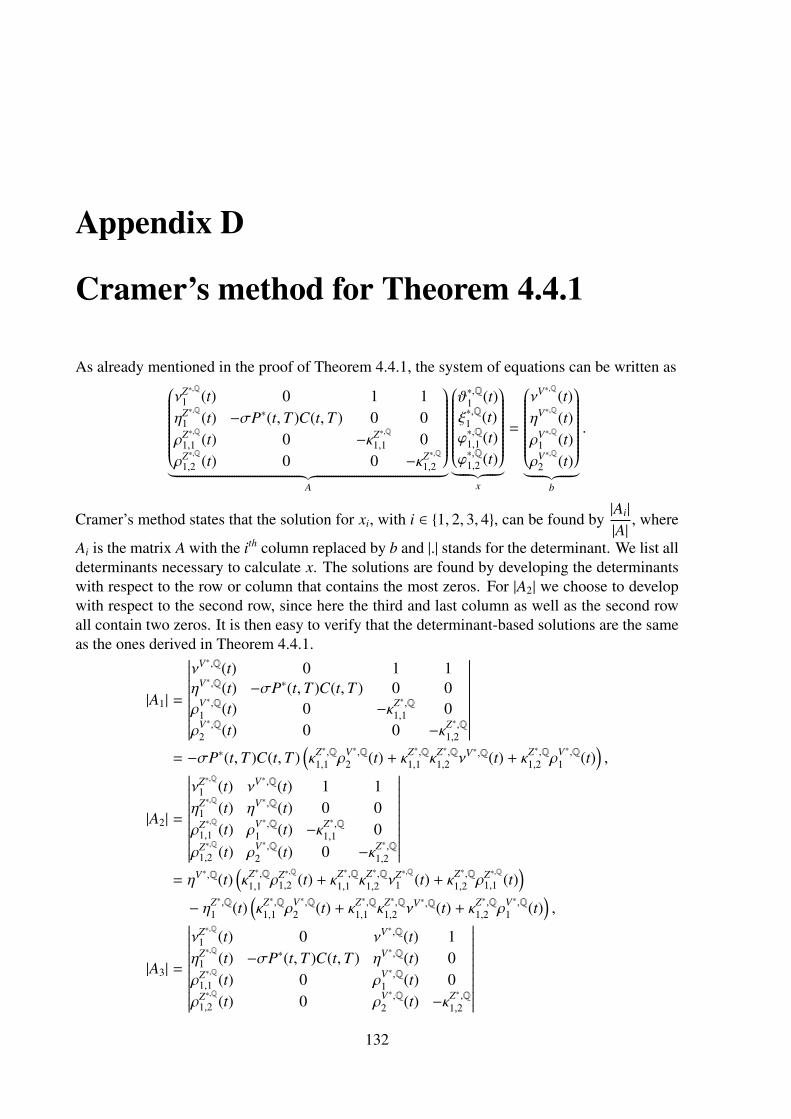
Appendix D
Cramer’s method for Theorem 4.4.1
As already mentioned in the proof of Theorem 4.4.1, the system of equations can be written asνZ∗,Q
1 (t) 0 1 1ηZ∗,Q
1 (t) −σP∗(t,T )C(t,T ) 0 0ρZ∗,Q
1,1 (t) 0 −κZ∗,Q1,1 0
ρZ∗,Q1,2 (t) 0 0 −κZ∗,Q
1,2
︸ ︷︷ ︸A
ϑ∗,Q1 (t)ξ∗,Q1 (t)ϕ∗,Q1,1 (t)ϕ∗,Q1,2 (t)
︸ ︷︷ ︸x
=
νV∗,Q(t)ηV∗,Q(t)ρV∗,Q
1 (t)ρV∗,Q
2 (t)
︸ ︷︷ ︸b
.
Cramer’s method states that the solution for xi, with i ∈ 1, 2, 3, 4, can be found by|Ai|
|A|, where
Ai is the matrix A with the ith column replaced by b and |.| stands for the determinant. We list alldeterminants necessary to calculate x. The solutions are found by developing the determinantswith respect to the row or column that contains the most zeros. For |A2| we choose to developwith respect to the second row, since here the third and last column as well as the second rowall contain two zeros. It is then easy to verify that the determinant-based solutions are the sameas the ones derived in Theorem 4.4.1.
|A1| =
∣∣∣∣∣∣∣∣∣∣∣∣νV∗,Q(t) 0 1 1ηV∗,Q(t) −σP∗(t,T )C(t,T ) 0 0ρV∗,Q
1 (t) 0 −κZ∗,Q1,1 0
ρV∗,Q2 (t) 0 0 −κZ∗,Q
1,2
∣∣∣∣∣∣∣∣∣∣∣∣= −σP∗(t,T )C(t,T )
(κZ∗,Q
1,1 ρV∗,Q2 (t) + κZ∗,Q
1,1 κZ∗,Q1,2 νV∗,Q(t) + κZ∗,Q
1,2 ρV∗,Q1 (t)
),
|A2| =
∣∣∣∣∣∣∣∣∣∣∣∣∣νZ∗,Q
1 (t) νV∗,Q(t) 1 1ηZ∗,Q
1 (t) ηV∗,Q(t) 0 0ρZ∗,Q
1,1 (t) ρV∗,Q1 (t) −κZ∗,Q
1,1 0ρZ∗,Q
1,2 (t) ρV∗,Q2 (t) 0 −κZ∗,Q
1,2
∣∣∣∣∣∣∣∣∣∣∣∣∣= ηV∗,Q(t)
(κZ∗,Q
1,1 ρZ∗,Q1,2 (t) + κZ∗,Q
1,1 κZ∗,Q1,2 νZ∗,Q
1 (t) + κZ∗,Q1,2 ρZ∗,Q
1,1 (t))
− ηZ∗,Q1 (t)
(κZ∗,Q
1,1 ρV∗,Q2 (t) + κZ∗,Q
1,1 κZ∗,Q1,2 νV∗,Q(t) + κZ∗,Q
1,2 ρV∗,Q1 (t)
),
|A3| =
∣∣∣∣∣∣∣∣∣∣∣∣∣νZ∗,Q
1 (t) 0 νV∗,Q(t) 1ηZ∗,Q
1 (t) −σP∗(t,T )C(t,T ) ηV∗,Q(t) 0ρZ∗,Q
1,1 (t) 0 ρV∗,Q1 (t) 0
ρZ∗,Q1,2 (t) 0 ρV∗,Q
2 (t) −κZ∗,Q1,2
∣∣∣∣∣∣∣∣∣∣∣∣∣132
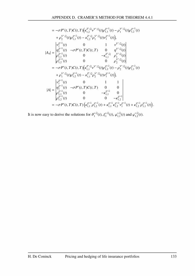
APPENDIX D. CRAMER’S METHOD FOR THEOREM 4.4.1
= −σP∗(t,T )C(t,T )(κZ∗,Q
1,2 νV∗,Q(t)ρZ∗,Q1,1 (t) − ρV∗,Q
1 (t)ρZ∗,Q1,2 (t)
+ ρV∗,Q2 (t)ρZ∗,Q
1,1 (t) − κZ∗,Q1,2 ρV∗,Q
1 (t)νZ∗,Q1 (t)
),
|A4| =
∣∣∣∣∣∣∣∣∣∣∣∣∣νZ∗,Q
1 (t) 0 1 νV∗,Q(t)ηZ∗,Q
1 (t) −σP∗(t,T )C(t,T ) 0 ηV∗,Q(t)ρZ∗,Q
1,1 (t) 0 −κZ∗,Q1,1 ρV∗,Q
1 (t)ρZ∗,Q
1,2 (t) 0 0 ρV∗,Q2 (t)
∣∣∣∣∣∣∣∣∣∣∣∣∣= −σP∗(t,T )C(t,T )
(κZ∗,Q
1,1 νV∗,Q(t)ρZ∗,Q1,2 (t) − ρV∗,Q
2 (t)ρZ∗,Q1,1 (t)
+ ρV∗,Q1 (t)ρZ∗,Q
1,2 (t) − κZ∗,Q1,1 ρV∗,Q
2 (t)νZ∗,Q1 (t)
),
|A| =
∣∣∣∣∣∣∣∣∣∣∣∣∣νZ∗,Q
1 (t) 0 1 1ηZ∗,Q
1 (t) −σP∗(t,T )C(t,T ) 0 0ρZ∗,Q
1,1 (t) 0 −κZ∗,Q1,1 0
ρZ∗,Q1,2 (t) 0 0 −κZ∗,Q
1,2
∣∣∣∣∣∣∣∣∣∣∣∣∣= −σP∗(t,T )C(t,T )
(κZ∗,Q
1,1 ρZ∗,Q1,2 (t) + κZ∗,Q
1,1 κZ∗,Q1,2 ν
Z∗,Q1 (t) + κZ∗,Q
1,2 ρZ∗,Q1,1 (t)
).
It is now easy to derive the solutions for ϑ∗,Q1 (t), ξ∗,Q1 (t), ϕ∗,Q1,1 (t) and ϕ∗,Q1,2 (t).
H. De Coninck Pricing and hedging of life insurance portfolios 133
Bibliography
K. K. Aase. Contingent claims valuation when the security price is a combination of an Itoprocess and a random point process. Stochastic processes and their applications, 28(2):185–220, 1988.
D. Applebaum. Levy processes and stochastic calculus. Cambridge University Press, 2004.
J. Barbarin. Heath-Jarrow-Morton modelling of longevity bonds and the risk-minimization oflife insurance portfolios. Insurance: Mathematics and Economics, 43(1):41–55, 2008.
T. Bjork. Arbitrage theory in continuous time. Oxford University Press, 3rd edition, 2009.
P. Bremaud. Point processes and queues, martingale dynamics. Springer, 1981.
R. Carmona. Indifference pricing: theory and applications. Princeton University Press, 2009.
A. Chen. Loss analysis of a life insurance company applying discrete-time risk-minimizinghedging strategies. Insurance: Mathematics and Economics, 42(3):1035–1049, 2008.
R. Cont and P. Tankov. Financial modelling with jump processes. CRC Press LLC, 2004.
M. Dahl. Stochastic mortality in life insurance: market reserve and mortality-linked insurancecontracts. Insurance: Mathematics and Economics, 35:113–136, 2004.
M. Dahl, M. Melchior, and T. Møller. On systematic mortality risk and risk-minimization withsurvivor swaps. Scandinavian Actuarial Journal, 2008(2-3):114–146, 2008.
M. Dahl, S. Glar, and T. Møller. Mixed dynamic and static risk-minimization with an applicationto survivor swaps. European Actuarial Journal, 1(2):233–260, 2011.
G. Di Nunno, B. Øksendal, and F. Proske. Malliavin calculus for Levy processes with applica-tions to finance. Springer, 2009.
H. Follmer and M. Schweizer. Hedging by sequential regression: an introduction to the math-ematics of option trading. ASTIN Bulletin, 19(1):29–42, 1989.
H. Follmer and D. Sondermann. Hedging of non-redundant contingent claims. Contributionsto Mathematical Economics: in honor of Gerard Debreu, pages 205–223, 1986.
N. Gatzert and H. Wesker. Mortality risk and its effect on shortfall and risk management in lifeinsurance. Journal of Risk and Insurance, 81(1):57–90, 2014.
134
BIBLIOGRAPHY
D. Hainaut and P. Devolder. Mortality modelling with Levy processes. Insurance: Mathematicsand Economics, 42(1):409–418, 2008.
J. Jacod and A. N. Shiryaev. Limit theorems for stochastic processes. Springer, 2nd edition,2003.
M.S. Joshi. The concepts and practice of mathematical finance. Cambridge University Press,2nd edition, 2008.
Y. Kahane. The theory of insurance risk premiums, a re-examination in the light of recentdevelopments in capital market theory. ASTIN Bulletin, 10(2):223–239, 1979.
D. Kahneman and A. Tversky. Prospect theory: an analysis of decision under risk. Economet-rica, 42(2):263–291, 1979.
M. Kaluszka and M. Krzeszowiec. Pricing insurance contracts under cumulative prospect the-ory. Insurance: Mathematics and Economics, 50:159–166, 2012.
U. Kuchler and M. Sørensen. Exponential families of stochastic processes. Springer, 1997.
T. Møller. Risk-minimizing hedging strategies for insurance payment processes. Finance andStochastics, 5:419–446, 2001.
P. E. Protter. Stochastic Integration and Differential Equations. Springer, 2nd edition, 2004.
K. Sato. Levy processes and infinitely divisible distributions. Cambridge University Press,1999.
S. E. Shreve. Stochastic calculus for finance I: the binomial asset pricing model. Springer,2004a.
S. E. Shreve. Stochastic calculus for finance II: continuous-time models. Springer, 2004b.
A. Tsanakas and E. Desli. Measurement and pricing of risk in insurance markets. Risk Analysis,25(6):1653–1668, 2005.
H. De Coninck Pricing and hedging of life insurance portfolios 135