GFM-Based Methods for Speaker Identification

This article has been accepted for inclusion in a future issue of this journal. Content is final as presented, with the exception of pagination.

IEEE TRANSACTIONS ON SYSTEMS, MAN, AND CYBERNETICS—PART B: CYBERNETICS 1

GFM-Based Methods for Speaker IdentificationSaurabh Bhardwaj, Smriti Srivastava, Member, IEEE, Madasu Hanmandlu, Senior Member, IEEE, and

J. R. P. Gupta, Senior Member, IEEE

Abstract—This paper presents three novel methods for speakeridentification of which two methods utilize both the continuousdensity hidden Markov model (HMM) and the generalized fuzzymodel (GFM), which has the advantages of both Mamdani andTakagi–Sugeno models. In the first method, the HMM is utilizedfor the extraction of shape-based batch feature vector that isfitted with the GFM to identify the speaker. On the other hand,the second method makes use of the Gaussian mixture model(GMM) and the GFM for the identification of speakers. Finally,the third method has been inspired by the way humans cash inon the mutual acquaintances while identifying a speaker. To seethe validity of the proposed models [HMM–GFM, GMM–GFM,and HMM–GFM (fusion)] in a real-life scenario, they are testedon VoxForge speech corpus and on the subset of the 2003 NationalInstitute of Standards and Technology evaluation data set. Thesemodels are also evaluated on the corrupted VoxForge speechcorpus by mixing with different types of noisy signals at differentvalues of signal-to-noise ratios, and their performance is foundsuperior to that of the well-known models.

Index Terms—Gaussian mixture model (GMM), generalizedfuzzy model (GFM), hidden Markov model (HMM), shape-basedbatching (SBB).

I. INTRODUCTION

THERE are a number of situations in which correct recog-nition of persons is required. The use of biometric-based

(physiological and/or behavioral characteristics of a person)recognition is the most “natural” way of recognizing a person.This is also very safe as these characteristics cannot be stolenor forgotten. Speaker recognition can be categorized into twospecific tasks: identification and verification. Speaker identifi-cation deals with which one of the known voices best matchesthe input voice sample, whereas speaker verification dealswith accepting or rejecting the identity claim of a speaker. Asobserved in [1], identification is also a very critical componentin negative recognition applications. The purpose of negativerecognition is to prevent a single person from using multipleidentities.

This paper describes the text-independent speaker identifica-tion system. Unlike iris patterns, fingerprints, DNA structures,

Manuscript received December 30, 2011; revised June 1, 2012 andSeptember 17, 2012; accepted September 27, 2012. This paper was recom-mended by Associate Editor C.-T. Lin.

S. Bhardwaj and S. Srivastava are with the Netaji Subhas Institute ofTechnology, University of Delhi, New Delhi 110 078, India.

M. Hanmandlu is with the Indian Institute of Technology Delhi, New Delhi110016, India.

J. R. P. Gupta is with the Department of Instrumentation and ControlEngineering, University of Delhi, Delhi 110 007, India.

Color versions of one or more of the figures in this paper are available onlineat http://ieeexplore.ieee.org.

Digital Object Identifier 10.1109/TSMCB.2012.2223461

and face recognition, speech is a behavioral biometric usedfor speaker identification. One of the benefits of using speechover other biometrics is that it contains both the physiologicaland behavioral characteristics of humans. It serves as a cue fordetermining the identity of a speaker. In contrast to other bio-metric signals, speech can be used remotely as it can be easilytransmitted over telephonic lines. A speech utterance from anunknown speaker is examined with the help of speech modelsof the known speakers. Hence, the speaker identification systemmakes a one-to-many comparisons to establish the identity ofan individual. The unknown speaker is identified when theknown model of a speaker matches the input utterances. Theapplications of speaker identification include access control,telephone shopping, transaction authorization, voice dialing,and remote access to computers. The statistical classifiers forthe identification of speakers are vector quantization (VQ)[2], the Gaussian mixture model (GMM) [3], and the hiddenMarkov model (HMM) [4]. The GMM-based approaches as-sume that the feature vectors follow the Gaussian distributioncharacterized by the mean and variance. The reason behind thewide use of GMM is explained in [5].

With the incorporation of the continuous density HMM(CDHMM), the state concept enters into the GMM. In thespeaker identification, the vocal tract at any time is in one ofa finite number of articulatory states. It produces a short signalhaving a finite number of prototypical spectra in every state.Thus, the power spectra of the speech signal are determinedsolely by the current state of the model, whereas the variation inthe spectral composition of the signal is determined by the statetransition law of the underlying Markov chain, which reflectsthe dynamic aspects of the speech, such as speaking style. Thedynamic nature of the speech signal necessitates the use of theHMM [6].

Initially, an ergodic discrete five-state HMM was used fortext-independent speaker recognition in [7], which was furtherextended in [8] using an eight-state ergodic autoregressive (AR)HMM. In this model, states were the linear combination of ARsources. Matsui and Furui [4] demonstrate the effectivenessof HMM-based speaker recognition methods over VQ-basedmethods. They also make a comparison between the HMMand the discrete HMM (DHMM) and find that the HMM is farsuperior to the DHHM. One important observation is that therecognition rate is dependent on the total number of mixtures,irrespective of the number of states. The recognition rate isfurther improved by using a combination of a Cochler filterand the HMM in [9]. Not much work is reported on thespeaker identification using fuzzy logic techniques, althoughthey are shown to be effective [10]. Fuzzy set theory wasfound suitable for classifying the vowels in [11]. For the

1083-4419/$31.00 © 2012 IEEE


2 IEEE TRANSACTIONS ON SYSTEMS, MAN, AND CYBERNETICS—PART B: CYBERNETICS

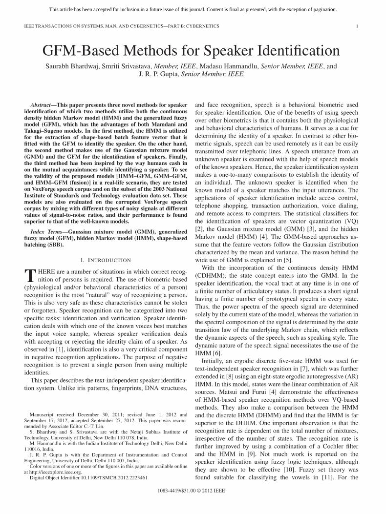
Fig. 1. Extraction of MFCCs.

text-independent speaker recognition, it is difficult to im-plement a single classifier that exhibits sufficiently highperformance in practical applications. Therefore, the fusionof multiple information sources is an option in speakeridentification [12].

Improved results are possible with a combination of a fewclassifiers [13], [14] such as the combination of statistical andsoft-computing paradigms. This is attempted in this paper byway of amalgamating the statistical tool HMM with the soft-computing tool general fuzzy model (GFM).

The task of speaker recognition is a subset of pattern recog-nition. In this paper, we capitalize the strong pattern recognitionability of the HMM in the shape-based batching (SBB) and thestrong generalization capability of the GFM in the identificationof speakers.

This paper is organized as follows. Section II describes theextraction of features for the speaker recognition, i.e., a briefintroduction to the HMM and the CDHMM. Section III reviewsthe concepts of the GFM. Section IV describes the proposedapproaches for the speaker identification. The experimentalresults are presented in Section V, and conclusions are givenin Section VI.

II. MODULES FOR SPEAKER RECOGNITION

All speaker recognition systems contain two main modules:feature extraction and feature matching. Feature extraction isthe process that extracts information from a voice signal of aspeaker. Feature matching is the procedure used to identify theunknown speaker by comparing his features with those of theknown speakers.

A. Feature Extraction

The best features to represent the speech signal for a speakerrecognition task are based on spectral analysis, and to mentionthe well-known features, we may cite linear predictive codingand Mel-frequency cepstral coefficients (MFCC). The proce-dure for extracting the MFCC coefficients is given in Fig. 1.

As part of the frame blocking, the continuous speech isblocked into frames of N samples, with adjacent frames beingseparated by M samples. Next, a Hamming window is used topartition each frame, and then a fast Fourier transform (FFT)

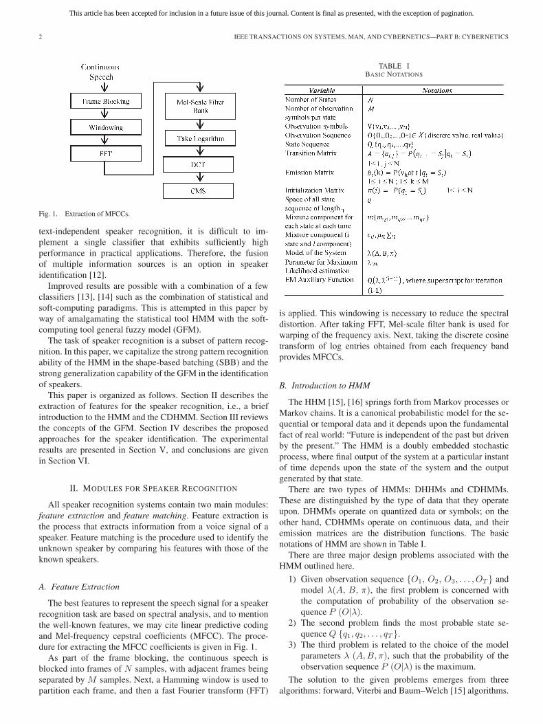
TABLE IBASIC NOTATIONS

is applied. This windowing is necessary to reduce the spectraldistortion. After taking FFT, Mel-scale filter bank is used forwarping of the frequency axis. Next, taking the discrete cosinetransform of log entries obtained from each frequency bandprovides MFCCs.

B. Introduction to HMM

The HHM [15], [16] springs forth from Markov processes orMarkov chains. It is a canonical probabilistic model for the se-quential or temporal data and it depends upon the fundamentalfact of real world: “Future is independent of the past but drivenby the present.” The HMM is a doubly embedded stochasticprocess, where final output of the system at a particular instantof time depends upon the state of the system and the outputgenerated by that state.

There are two types of HMMs: DHHMs and CDHMMs.These are distinguished by the type of data that they operateupon. DHMMs operate on quantized data or symbols; on theother hand, CDHMMs operate on continuous data, and theiremission matrices are the distribution functions. The basicnotations of HMM are shown in Table I.

There are three major design problems associated with theHMM outlined here.

1) Given observation sequence {O1, O2, O3, . . . , OT } andmodel λ(A, B, π), the first problem is concerned withthe computation of probability of the observation se-quence P (O|λ).

2) The second problem finds the most probable state se-quence Q {q1, q2, . . . , qT }.

3) The third problem is related to the choice of the modelparameters λ (A,B, π), such that the probability of theobservation sequence P (O|λ) is the maximum.

The solution to the given problems emerges from threealgorithms: forward, Viterbi and Baum–Welch [15] algorithms.


BHARDWAJ et al.: GFM-BASED METHODS FOR SPEAKER IDENTIFICATION 3

1) CDHMM: Let O = {O1, O2, . . . , OT } be the observa-tion sequence and Q {q1, q2, . . . , qT } be the hidden statesequence. We now brief the expectation–maximization (EM)algorithm for finding the maximum-likelihood estimate of theparameters of an HMM given a set of observed feature vectors.The Q function is generally defined as

Q(λ, λ(i−1)) = Σq∈� logP (O, Q|λ)P (O, Q|λ(i−1)). (1)

The expectation step (E-step) and the maximization (M-step) ofthe EM algorithm are as follows:

E Step:

ΣQ∈�Σm∈M logP (O, Qm|λ)P (O, Qm|λi−1). (2)

M Step:

λ(i) = argmaxλ

[Q(λ, λ(i−1))

]+ constraint. (3)

The final result is that, when i → ∞, λ(i−1) → λML.The optimized equations for the parameters of the mixture

density are [16] as follows:

μil =ΣT

t=1OtP (qt = i,mqt = l|O, λ(i−1))

ΣTt=1P (qt = i,mqtt

= l|O, λ(i−1))(4)

Σil=ΣT

t=1(Ot−μil)(Ot−μil)TP (qt=i,mqtt

=l|O, λ(i−1))

ΣTt=1P (qt = i,mqtt

= l|O, λ(i−1))(5)

cil =ΣT

t=1P (qt = i,mqtt= l|O, λ(i−1))

ΣTt=1Σ

Ml=1P (qt = i,mqtt

= l|O, λ(i−1)). (6)

III. GFM

There are three types of Fuzzy models: the Mamdani–Larsen(ML) model [17], [18], the Takagi–Sugeno (TS) model [19],and the GFM proposed in [20]. It may be seen that the IF partsof all the three rules are the same, except their consequent parts.The rules for ML and TS models are as follows.Rk (ML):

IFx1 isAk1 ∧ x2 isAk

2 . . . ∧ xD isAkD THENy isBk(bk, vk)

(7)Rk (TS):

IFx1 isAk1 ∧ x2 isAk

2 . . . ∧ xD isAkD THENy is fk(x) (8)

where

fk(x) = bk0 + bk1x1+ · · ·+ bkDxD

From (7) and (8), we find that each ML rule maps the fuzzy setsin the input space Ak to a fuzzy set Bk in the output space,whereas the TS model relates the fuzzy sets in the input spaceto the functional relationship in the output space.

The GFM combines the properties of both ML and TSmodels. It has the output fuzzy set in the form Bk(fk(x), vk)with a varying centroid fk(x) [in contrast to ML that has a static

centroid (bk)], and an index of “fuzziness,” quantified by vk(incontrast to TS that is a singleton), as follows:

Rk(GFM) : IFx1 isAk1 ∧ x2 . . . . . . ∧ xD isAk

D

THEN y isBk

(fk(x), vk

). (9)

The firing strength of the kth rule, which is taken as the fuzzyconjunction (denoted by ∧) of the membership functions of arule’s IF part, is

μk(x) = μk1(x1) ∧ μk

2(x2), . . . , μkD(xD) (10)

where μkd(xd) is the membership function of the fuzzy set Ak

d .The defuzzified outputs using the weighted average method forthe above three methods can be found as

yo =ΣKk=1

μk(x).vkΣK

k′=1μk′(x).vk′

.bk (11)

yo =ΣKk=1

μk(x)

ΣKk′=1μ

k′(x).fk(x) (12)

yo =ΣKk=1

μk(x).vkΣK

k′=1μk′(x).vk′

.fk(x). (13)

IV. PROPOSED METHODS

We now present three methods for the identification of speak-ers. A notable point is that all three methods have the GFM asa common thread. These methods are applied on the VoxForgedatabase of 40 speakers, although it has 100 speakers, for easeof illustration.

A. Log-Likelihood-Based HMM–GFM Method

In the automatic speaker recognition, a speaker is treatedas a black box generating the feature vectors. After extractingthe MFCC of test speech data (training data), the featurescorresponding to all speakers in the database are appended toform one array, which is subsequently modeled by the HMMmodel. Note that the random speech source [21] has hiddenstates that represent the characteristic vocal-tract configura-tions. The random source produces spectral feature vectorsfrom the associated vocal-tract configuration according to amultidimensional Gaussian probability density function (pdf).The pdf of state j as a function of the D-dimensional featurevector x is expressed as

Pj(x)=1

(2π)D2 |Σj |

12

× exp

{−12(x− μj)

T (Σj)−1(x− μj)

}

(14)where μj is the state mean vector, and Σj is the state covari-ance matrix. The mean vector represents the expected spectralfeature vector of the state, and the covariance matrix representsthe correlations and variability of spectral features within thestate.

We will furnish the arguments in favor of SBBs. Generally,different distance functions such as Euclidean distance, Man-hattan distance, and cosine distance are employed for clustering



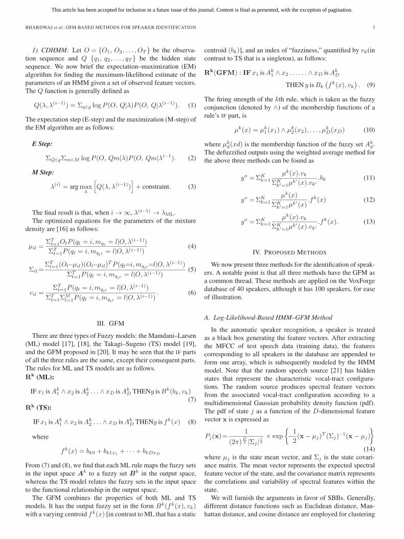
Fig. 2. Clustering results with the segmental k-means

TABLE IICORRELATION COEFFICIENTS

the data, but these distance functions are not always effectiveto capture the correlations among the objects. In fact, strongcorrelations may still exist among a set of objects even ifthe distances from each other, as measured by the distancefunctions, are far apart. Fig. 2 shows four objects with tenattributes among a set of 300 objects, which is allotted indifferent clusters when the k-means clustering is applied topartition them into six clusters. As shown from the figure, theseobjects have the same shape. The strong correlation among fourdata elements is shown with the help of correlation matrix inTable II. The GFM finds it much easier to analyze the signalsbased on their shape; therefore, taking the clue from here, wehave extended the basic concept of SBB introduced in [22]–[24]for clustering the speech data. It is possible to find the shape ofthe data sets from their log likelihoods (LLs), although it is notalways easy. Moreover, in some data sets, it is impossible todetermine the threshold for allocating a batch to a data set.

Although the states are hidden, some physical significanceis often attached to the states of the model in many practicalapplications. Any data representing a particular state is foundto possess the similar shape as against the data representinganother state. Therefore, in the SBB, the shape is consideredas a function of the state rather than the LL.

As part of HMM modeling and in conjunction with SBB, westart with the initialization of HMM parameters. After this, thenext step is to find the optimal state sequence with the help of“Viterbi algorithm” by considering the entire input data set asthe D-dimensional observation vector sequence. Having boththe observation sequence and the corresponding state sequence,we note that the data vectors associated with the same statehave an identical shape, whereas the data vectors associatedwith different states have no similarity in their shapes. Once theoptimal value of the hidden state sequence is deduced, the nextstep is to group the data into batches according to their state.Since each batch has an almost identical shape, it is difficult to

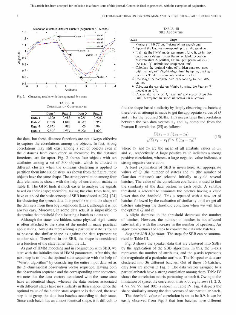
TABLE IIISBB ALGORITHM

find the shape-based similarity by simply observing the batches;therefore, an attempt is made to get the appropriate values of Qand m for the required SBBs. This necessitates the correlationbetween the two data vectors x1 and x2 computed from thePearson R correlation [25] as follows:

Σ(x1 − x̄1)(x2 − x̄2)√Σ(x1 − x̄1)2 × Σ(x2 − x̄2)2

(15)

where x1 and x2 are the mean of all attribute values in x1

and x2, respectively. A large positive value indicates a strongpositive correlation, whereas a large negative value indicates astrong negative correlation.

A brief explanation of SBB is given here. An appropriatevalues of Q (the number of states) and m (the number ofGaussian mixtures) are selected initially to yield severalbatches. The value of the correlation coefficient is used to findthe similarity of the data vectors in each batch. A suitablethreshold is selected to eliminate the batches having a valuelower than the threshold. This is repeated with a new set ofbatches followed by the evaluation of similarity until we get allbatches satisfying the threshold condition when we will havethe optimal Q and m.

A slight decrease in the threshold decreases the numberof batches. However, the number of batches is not affectedsubstantially with the increase in the number of speakers. Analgorithm outlines the steps to convert the data into batches.

Steps for SBB Algorithm: The steps for SBB can be summa-rized in Table III.

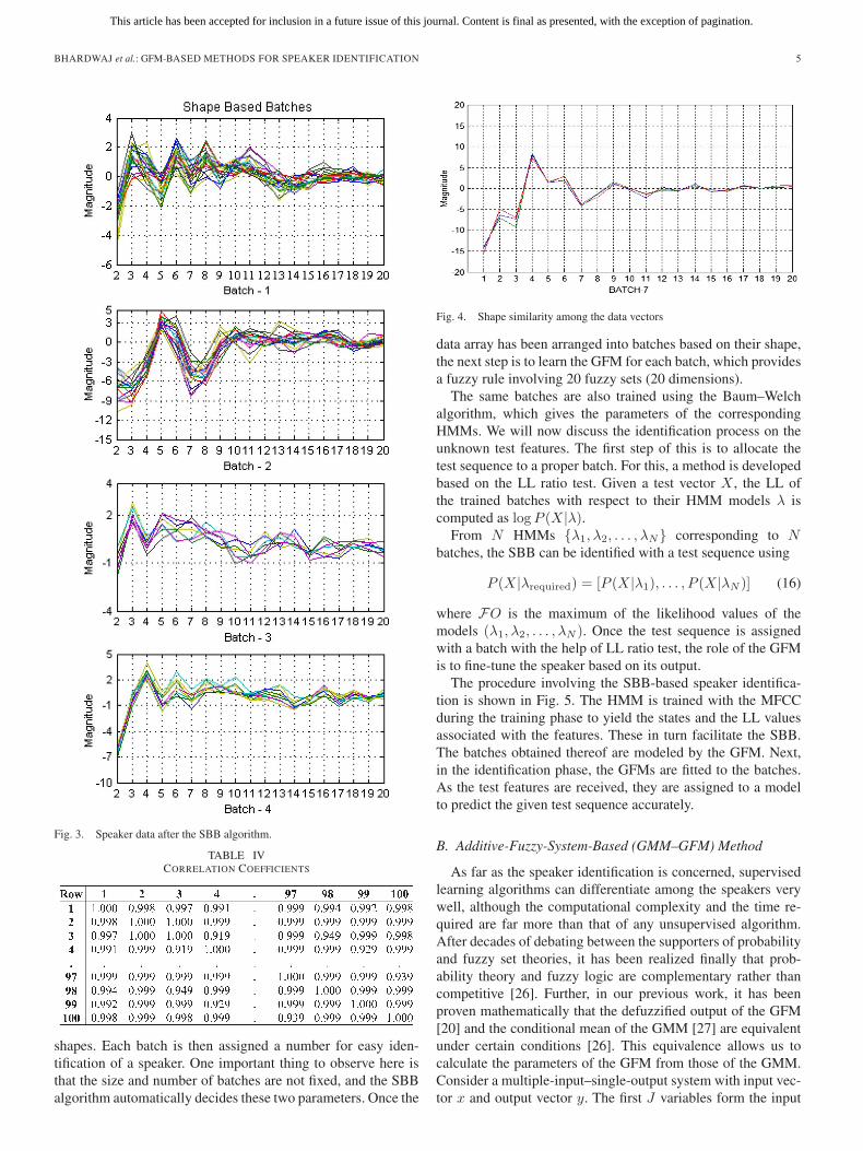
Fig. 3 shows the speaker data that are clustered into SBBsby the application of the SBB algorithm. In this, the x-axisrepresents the number of attributes, and the y-axis representsthe magnitude of a particular attribute. The 40-speaker data areclustered into 36 different batches. Out of these 36 batches,only four are shown in Fig. 3. The data vectors assigned to aparticular batch have a strong correlation among them. Table IVshows the correlation matrix pertaining to batch 6. Owing to thelimitation of space, the correlation matrix of eight rows (1, 2, 3,4, 97, 98, 99, and 100) is shown in Table IV. Fig. 4 depicts theshape similarity among the data vectors of one particular batch.

The threshold value of correlation is set to be 0.9. It can beeasily observed from Fig. 3 that four batches have different



Fig. 3. Speaker data after the SBB algorithm.

TABLE IVCORRELATION COEFFICIENTS

shapes. Each batch is then assigned a number for easy iden-tification of a speaker. One important thing to observe here isthat the size and number of batches are not fixed, and the SBBalgorithm automatically decides these two parameters. Once the

Fig. 4. Shape similarity among the data vectors

data array has been arranged into batches based on their shape,the next step is to learn the GFM for each batch, which providesa fuzzy rule involving 20 fuzzy sets (20 dimensions).

The same batches are also trained using the Baum–Welchalgorithm, which gives the parameters of the correspondingHMMs. We will now discuss the identification process on theunknown test features. The first step of this is to allocate thetest sequence to a proper batch. For this, a method is developedbased on the LL ratio test. Given a test vector X , the LL ofthe trained batches with respect to their HMM models λ iscomputed as logP (X|λ).

From N HMMs {λ1, λ2, . . . , λN} corresponding to Nbatches, the SBB can be identified with a test sequence using

P (X|λrequired) = [P (X|λ1), . . . , P (X|λN )] (16)

where FO is the maximum of the likelihood values of themodels (λ1, λ2, . . . , λN ). Once the test sequence is assignedwith a batch with the help of LL ratio test, the role of the GFMis to fine-tune the speaker based on its output.

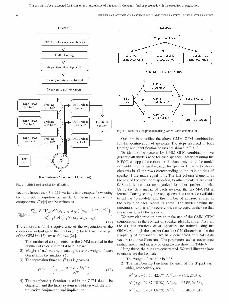
The procedure involving the SBB-based speaker identifica-tion is shown in Fig. 5. The HMM is trained with the MFCCduring the training phase to yield the states and the LL valuesassociated with the features. These in turn facilitate the SBB.The batches obtained thereof are modeled by the GFM. Next,in the identification phase, the GFMs are fitted to the batches.As the test features are received, they are assigned to a modelto predict the given test sequence accurately.

B. Additive-Fuzzy-System-Based (GMM–GFM) Method

As far as the speaker identification is concerned, supervisedlearning algorithms can differentiate among the speakers verywell, although the computational complexity and the time re-quired are far more than that of any unsupervised algorithm.After decades of debating between the supporters of probabilityand fuzzy set theories, it has been realized finally that prob-ability theory and fuzzy logic are complementary rather thancompetitive [26]. Further, in our previous work, it has beenproven mathematically that the defuzzified output of the GFM[20] and the conditional mean of the GMM [27] are equivalentunder certain conditions [26]. This equivalence allows us tocalculate the parameters of the GFM from those of the GMM.Consider a multiple-input–single-output system with input vec-tor x and output vector y. The first J variables form the input



Fig. 5. SBB-based speaker identification.

vector, whereas the (J + 1)th variable is the output. Now, usingthe joint pdf of input–output as the Gaussian mixture with ccomponents, E[y|x] can be written as

E[y|x]=ΣC

c=1PcΠJj=1N

J (xj , μcj , σcjj)(μcy − [x−μcx]′σxy

c

σyyc

)ΣC

c′=1Pc′ΠJj=1N

J(xj , μc′j , σc′jj).

(17)The conditions for the equivalence of the expectation of theconditional output given the input in (17) due to t and the outputof the GFM in (13), are as follows [26].

1) The number of components c in the GMM is equal to thenumber of rules k in the GFM rule base.

2) Weight of each rule vk is analogous to the weight of eachGaussian in the mixture Pc.

3) The regression function fk(x) is given as

fk(x) =

(μcy −

[x− μcx]′σxyc

σyyc

). (18)

4) The membership functions used in the GFM should beGaussian, and the fuzzy system is additive with the mul-tiplicative conjunction and implication.

Fig. 6. Identification procedure using GMM–GFM combination.

Our aim is to utilize the above GMM–GFM combinationfor the identification of speakers. The steps involved in bothtraining and identification phases are shown in Fig. 6.

To identify the speaker by GMM–GFM combination, wegenerate 40 models (one for each speaker). After obtaining theMFCC, we append a column in the data array to aid the modelin identifying the speaker, e.g., for speaker 1, the last columnelements in all the rows corresponding to the training data ofspeaker 1 are made equal to 1. The last column elements inthe rest of the rows corresponding to other speakers are made0. Similarly, the data are organized for other speaker models.Using the data matrix of each speaker, the GMM–GFM islearned. During testing, the test speech data are made availableto all the 40 models, and the number of nonzero entries inthe output of each model is noted. The model having themaximum number of nonzero entries is selected as the one thatis associated with the speaker.

We now elaborate on how to make use of the GMM–GFMcombination in the context of speaker identification. First, allthe 40 data matrices of 40 speakers are trained using theGMM. Although the speaker data are of 20 dimensions, for thesimplicity of explanation, we have considered only 6-D datavectors and three Gaussians. The parameters such as covariancematrix, mean, and inverse covariance are shown in Table V.

Using these, the rules are constructed. We will illustrate howto enumerate the first rule.

1) The weight of this rule is 0.23.2) The membership functions for each of the IF part vari-

ables, respectively, are

N1(x1;−14.40, 42.47), N2(x2;−8.31, 23.63),

N3(x3;−02.87, 10.23), N4(x4;−02.58, 04.53),

N5(x5;−02.04, 05.79), N6(x6;−01.46, 01.31).



TABLE VPARAMETERS OF GMM–GFM

3) Function f1(x) is given by

0.99−

⎡⎢⎢⎢⎢⎢⎣

⎡⎢⎢⎢⎢⎢⎣

x1

x2

x3

x4

x5

x6

⎤⎥⎥⎥⎥⎥⎦−

⎡⎢⎢⎢⎢⎢⎣

−14.408.312.872.582.041.46

⎤⎥⎥⎥⎥⎥⎦

⎤⎥⎥⎥⎥⎥⎦

⎡⎢⎢⎢⎢⎢⎣

2.68−3.944.08−3.853.23−2.20

⎤⎥⎥⎥⎥⎥⎦

67.54.

The premise and the consequent parts of the rule are givenby (19). By following the above procedure, rules R2 and R3are calculated. To check the identity of the test features of anunknown speaker, the outputs of all the speaker models areevaluated, and the model with the highest output gives the useridentity.

C. LL-Based HMM–GFM (Fusion) Method

As in [21], the attributes are categorized as high-level cues,such as word usage and idiosyncrasies in pronunciation, andlow-level cues, such as soft or loud, clear or rough, and slow orfast attributes. The latter type is considered here. This methodis patterned after the way the humans identify a speaker. To un-derstand this method, consider the following case: Two friends

Fig. 7. Identification results for different initial conditions.

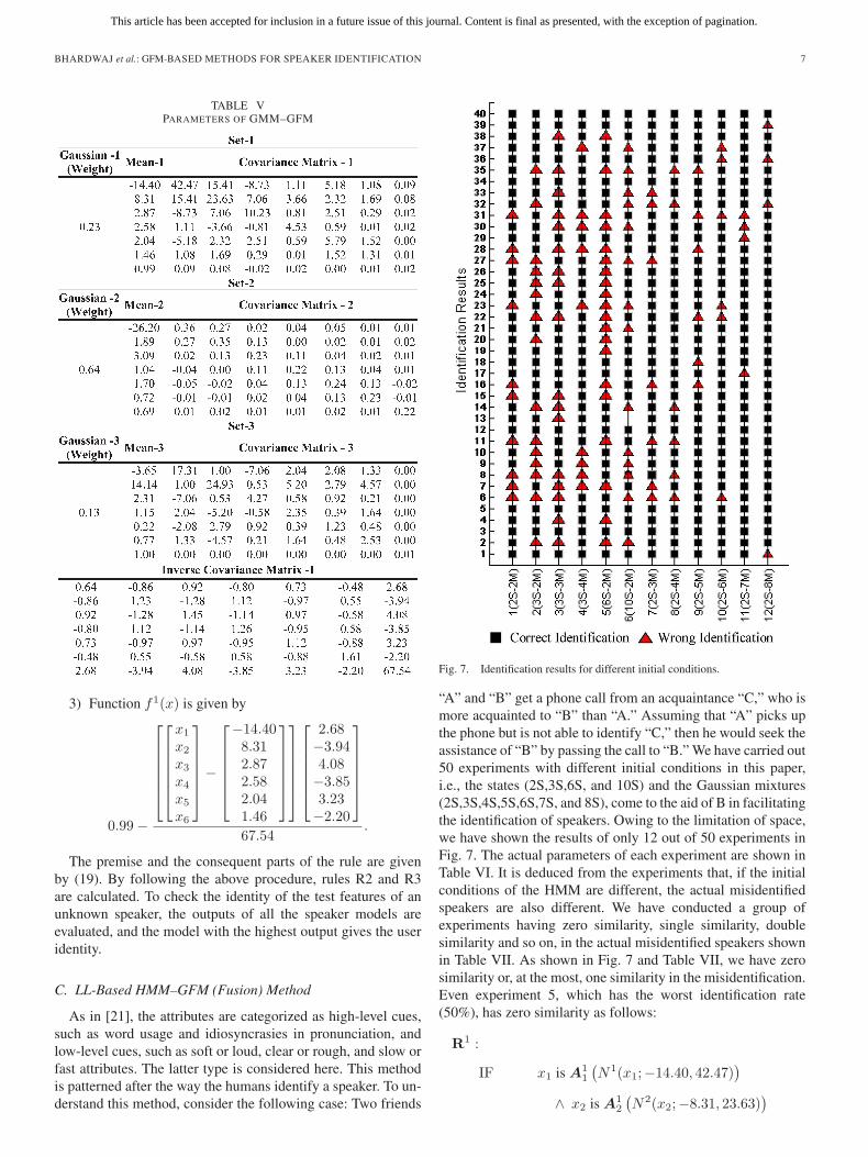
“A” and “B” get a phone call from an acquaintance “C,” who ismore acquainted to “B” than “A.” Assuming that “A” picks upthe phone but is not able to identify “C,” then he would seek theassistance of “B” by passing the call to “B.” We have carried out50 experiments with different initial conditions in this paper,i.e., the states (2S,3S,6S, and 10S) and the Gaussian mixtures(2S,3S,4S,5S,6S,7S, and 8S), come to the aid of B in facilitatingthe identification of speakers. Owing to the limitation of space,we have shown the results of only 12 out of 50 experiments inFig. 7. The actual parameters of each experiment are shown inTable VI. It is deduced from the experiments that, if the initialconditions of the HMM are different, the actual misidentifiedspeakers are also different. We have conducted a group ofexperiments having zero similarity, single similarity, doublesimilarity and so on, in the actual misidentified speakers shownin Table VII. As shown in Fig. 7 and Table VII, we have zerosimilarity or, at the most, one similarity in the misidentification.Even experiment 5, which has the worst identification rate(50%), has zero similarity as follows:

R1 :

IF x1 is A11

(N1(x1;−14.40, 42.47)

)∧ x2 is A1

2

(N2(x2;−8.31, 23.63)

)



TABLE VIEXPERIMENTS WITH DIFFERENT INITIAL CONDITIONS

TABLE VIIMISIDENTIFICATION SIMILARITY IN DIFFERENT EXPERIMENTS

∧ x3 is A13

(N3(x3;−02.87, 10.23)

)∧ x4 is A1

4

(N4(x4; 02.58, 04.53)

)∧ x5 is A1

5

(N5(x5;−02.04, 05.79)

)∧ x6 is A1

6

(N6(x6; 01.46, 01.31)

)THEN B1

(f1(x) = 9.92 exp(−3)− 0.039x1

+ 0.05x2 + 0.06x3 − 0.05x4

+ 0.04x5 − 0.03x6. (19)

From the above experimental results, a fusion method involvingboth HMM and GFM for the identification of speakers is pro-posed. Two sets of speaker models are considered to identify thespeakers. Each set consists of N HMM models correspondingto each speaker. The models of each set differ in their initialvalues, viz., the number of states and the number of Gaussiansused in the GMM. As explained earlier, speakers displayinga large variation in their speech signals under different initialconditions lead to misidentification.

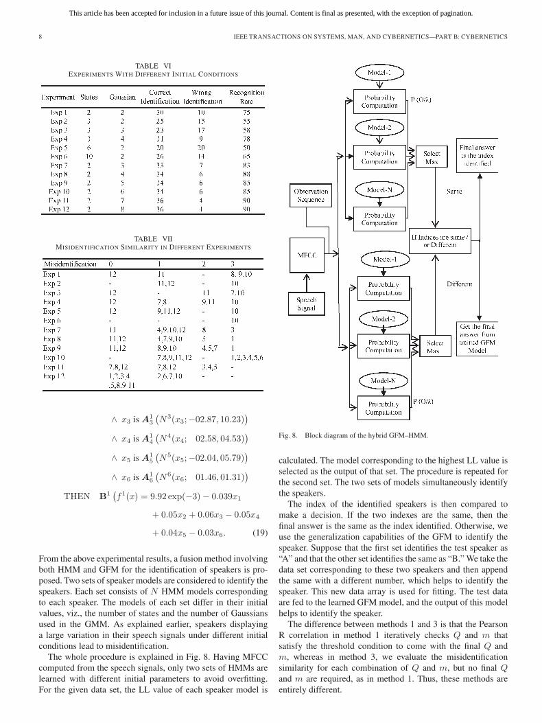
The whole procedure is explained in Fig. 8. Having MFCCcomputed from the speech signals, only two sets of HMMs arelearned with different initial parameters to avoid overfitting.For the given data set, the LL value of each speaker model is

Fig. 8. Block diagram of the hybrid GFM–HMM.

calculated. The model corresponding to the highest LL value isselected as the output of that set. The procedure is repeated forthe second set. The two sets of models simultaneously identifythe speakers.

The index of the identified speakers is then compared tomake a decision. If the two indexes are the same, then thefinal answer is the same as the index identified. Otherwise, weuse the generalization capabilities of the GFM to identify thespeaker. Suppose that the first set identifies the test speaker as“A” and that the other set identifies the same as “B.” We take thedata set corresponding to these two speakers and then appendthe same with a different number, which helps to identify thespeaker. This new data array is used for fitting. The test dataare fed to the learned GFM model, and the output of this modelhelps to identify the speaker.

The difference between methods 1 and 3 is that the PearsonR correlation in method 1 iteratively checks Q and m thatsatisfy the threshold condition to come with the final Q andm, whereas in method 3, we evaluate the misidentificationsimilarity for each combination of Q and m, but no final Qand m are required, as in method 1. Thus, these methods areentirely different.



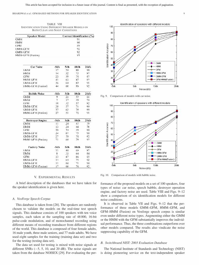
TABLE VIIIIDENTIFICATION USING DIFFERENT SPEAKER MODELS ON

BOTH CLEAN AND NOISY CONDITIONS

V. EXPERIMENTAL RESULTS

A brief description of the databases that we have taken forthe speaker identification is given here.

A. VoxForge Speech Corpus

This database is taken from [28]. The speakers are randomlychosen to validate the models on the real-time test speechsignals. This database consists of 100 speakers with ten voicesamples, each taken at the sampling rate of 48 000, 16-bitpulse-code modulation, and of monochannel recording usingdifferent means of recording transducer from different regionsof the world. This database is composed of four female adults,16 male youth, three male seniors, and 77 male adults. We haveused eight samples for the training (training data set) and twofor the testing (testing data set).

The data set used for testing is mixed with noise signals atdifferent SNRs (−5, 5, 10, and 20 dB). The noise signals aretaken from the database NOISEX [29]. For evaluating the per-

Fig. 9. Comparison of models with car noise.

Fig. 10. Comparison of models with babble noise.

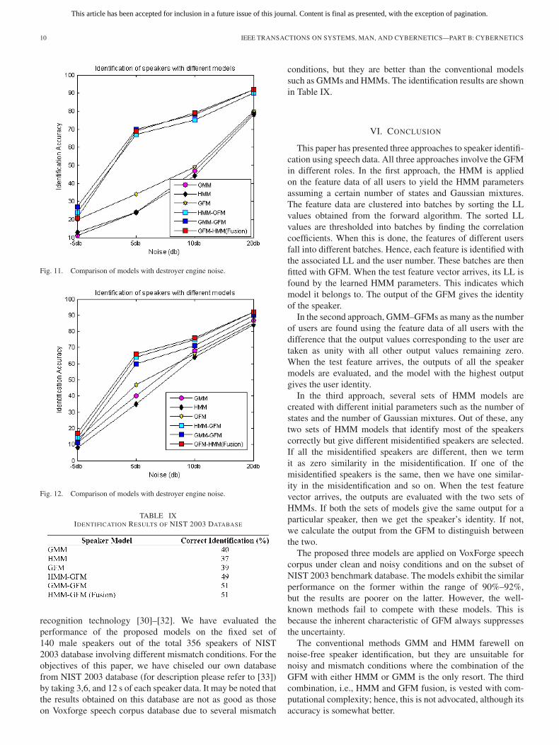
formance of the proposed models on a set of 100 speakers, fourtypes of noise: car noise, speech babble, destroyer operationengine, and factory noise are used. Table VIII and Figs. 9–12show a comparison of six identification models for differentnoise conditions.

It is observed in Table VII and Figs. 9–12 that the per-formance of three models GMM–GFM, HMM–GFM, andGFM–HMM (Fusion) on Voxforge speech corpus is similareven under different noise types. Augmenting either the GMMor the HMM with the GFM substantially improves the individ-ual performance. Thus, the three combinations outperform overother models compared. The results also vindicate the noisesuppressing capability of the GFM.

B. Switchboard NIST: 2003 Evaluation Database

The National Institute of Standards and Technology (NIST)is doing pioneering service on the text-independent speaker



Fig. 11. Comparison of models with destroyer engine noise.

Fig. 12. Comparison of models with destroyer engine noise.

TABLE IXIDENTIFICATION RESULTS OF NIST 2003 DATABASE

recognition technology [30]–[32]. We have evaluated theperformance of the proposed models on the fixed set of140 male speakers out of the total 356 speakers of NIST2003 database involving different mismatch conditions. For theobjectives of this paper, we have chiseled our own databasefrom NIST 2003 database (for description please refer to [33])by taking 3,6, and 12 s of each speaker data. It may be noted thatthe results obtained on this database are not as good as thoseon Voxforge speech corpus database due to several mismatch

conditions, but they are better than the conventional modelssuch as GMMs and HMMs. The identification results are shownin Table IX.

VI. CONCLUSION

This paper has presented three approaches to speaker identifi-cation using speech data. All three approaches involve the GFMin different roles. In the first approach, the HMM is appliedon the feature data of all users to yield the HMM parametersassuming a certain number of states and Gaussian mixtures.The feature data are clustered into batches by sorting the LLvalues obtained from the forward algorithm. The sorted LLvalues are thresholded into batches by finding the correlationcoefficients. When this is done, the features of different usersfall into different batches. Hence, each feature is identified withthe associated LL and the user number. These batches are thenfitted with GFM. When the test feature vector arrives, its LL isfound by the learned HMM parameters. This indicates whichmodel it belongs to. The output of the GFM gives the identityof the speaker.

In the second approach, GMM–GFMs as many as the numberof users are found using the feature data of all users with thedifference that the output values corresponding to the user aretaken as unity with all other output values remaining zero.When the test feature arrives, the outputs of all the speakermodels are evaluated, and the model with the highest outputgives the user identity.

In the third approach, several sets of HMM models arecreated with different initial parameters such as the number ofstates and the number of Gaussian mixtures. Out of these, anytwo sets of HMM models that identify most of the speakerscorrectly but give different misidentified speakers are selected.If all the misidentified speakers are different, then we termit as zero similarity in the misidentification. If one of themisidentified speakers is the same, then we have one similar-ity in the misidentification and so on. When the test featurevector arrives, the outputs are evaluated with the two sets ofHMMs. If both the sets of models give the same output for aparticular speaker, then we get the speaker’s identity. If not,we calculate the output from the GFM to distinguish betweenthe two.

The proposed three models are applied on VoxForge speechcorpus under clean and noisy conditions and on the subset ofNIST 2003 benchmark database. The models exhibit the similarperformance on the former within the range of 90%–92%,but the results are poorer on the latter. However, the well-known methods fail to compete with these models. This isbecause the inherent characteristic of GFM always suppressesthe uncertainty.

The conventional methods GMM and HMM farewell onnoise-free speaker identification, but they are unsuitable fornoisy and mismatch conditions where the combination of theGFM with either HMM or GMM is the only resort. The thirdcombination, i.e., HMM and GFM fusion, is vested with com-putational complexity; hence, this is not advocated, although itsaccuracy is somewhat better.



REFERENCES

[1] A. Jain, A. Ross, and S. Prabhakar, “An introduction to biometric recogni-tion,” IEEE Trans. Circuits Syst. Video Technol., vol. 14, no. 1, pp. 4–20,Jan. 2004.

[2] F. Soong, A. Rosenberg, L. Rabiner, and B. Juang, “A vector quantizationapproach to speaker recognition,” in Proc. IEEE ICASSP, 1985, vol. 10,pp. 387–390.

[3] D. Reynolds and R. Rose, “Robust text-independent speaker identifica-tion using Gaussian mixture speaker models,” IEEE Trans. Speech AudioProcess., vol. 3, no. 1, pp. 72–83, Jan. 1995.

[4] T. Matsui and S. Furui, “Comparison of text-independent speakerrecognition methods using vq-distortion and discrete/continuousHMMS,” in Proc. ICASSP, 1992, vol. 2, pp. 157–160.

[5] R. Togneri and D. Pullella, “An overview of speaker identification: Ac-curacy and robustness issues,” IEEE Circuits Syst. Mag., vol. 11, no. 2,pp. 23–61, Second Quarter, 2011.

[6] M. Deshpande and R. Holambe, “Text-independent speaker identificationusing hidden Markov models,” in Proc. 1st ICETET , 2008, pp. 641–644.

[7] A. Poritz, “Linear predictive hidden Markov models and the speech sig-nal,” in Proc. IEEE ICASSP, 1982, vol. 7, pp. 1291–1294.

[8] N. Tisby, “On the application of mixture ar hidden Markov models to textindependent speaker recognition,” IEEE Trans. Signal Process., vol. 39,no. 3, pp. 563–570, Mar. 1991.

[9] M. Inman, D. Danforth, S. Hangai, and K. Sato, “Speaker iden-tification using hidden Markov models,” in Proc. 4th IEEE ICSP, 1998,pp. 609–612.

[10] Z. Yuan, C. Yu, and Y. Fang, “Text independent speaker identification us-ing fuzzy mathematical algorithm,” in Proc. IEEE ICASSP, 1993, vol. 2,pp. 403–406.

[11] S. Pal and D. Majumder, “Fuzzy sets and decision making approachesin vowel and speaker recognition,” IEEE Trans. Syst., Man, Cybern,vol. SMC-7, no. 8, pp. 625–629, Aug. 1977.

[12] D. Mashao and M. Skosan, “Combining classifier decisions for robustspeaker identification,” Pattern Recognit., vol. 39, no. 1, pp. 147–155,Jan. 2006.

[13] H. Altinçay and M. Demirekler, “Speaker identification by combiningmultiple classifiers using dempster–shafer theory of evidence,” SpeechCommun., vol. 41, no. 4, pp. 531–547, Nov. 2003.

[14] S. Nakagawa, W. Zhang, and M. Takahashi, “Text-independent/text-prompted speaker recognition by combining speaker-specific gmm withspeaker adapted syllable-based hmm,” IEICE Trans. Inf. Syst., vol. 89,no. 3, pp. 1058–1065, Mar. 2006.

[15] L. Rabiner, “A tutorial on hidden Markov models and selected applica-tions in speech recognition,” Proc. IEEE, vol. 77, no. 2, pp. 257–286,Feb. 1989.

[16] J. Bilmes, “A gentle tutorial of the em algorithm and its application toparameter estimation for Gaussian mixture and hidden Markov models,”Int. Comput. Sci. Inst., vol. 4, no. 510, p. 126, 1998.

[17] E. Mamdani, “Application of fuzzy logic to approximate reasoningusing linguistic synthesis,” IEEE Trans. Comput., vol. C-26, no. 12,pp. 1182–1191, Dec. 1977.

[18] P. Martin Larsen, “Industrial applications of fuzzy logic control,” Int. J.Man-Mach. Stud., vol. 12, no. 1, pp. 3–10, Jan. 1980.

[19] T. Takagi and M. Sugeno, “Fuzzy identification of systems and its ap-plications to modeling and control,” IEEE Trans. Syst., Man Cybern.,vol. SMC-15, no. 1, pp. 116–132, Jan./Feb. 1985.

[20] M. Azeem, M. Hanmandlu, and N. Ahmad, “Generalization of adaptiveneuro-fuzzy inference systems,” IEEE Trans. Neural Netw., vol. 11, no. 6,pp. 1332–1346, Nov. 2000.

[21] D. Reynolds, “Automatic speaker recognition using Gaussian mixturespeaker models,” Lincoln Lab. J., vol. 8, no. 2, pp. 173–192, 1995.

[22] S. Srivastava, S. Bhardwaj, A. Madhvan, and J. Gupta, “A novel shapebased batching and prediction approach for time series using HMMS andFISS,” in Proc. 10th IEEE Int. Conf. ISDA, 2010, pp. 929–934.

[23] S. Bhardwaj, S. Srivastava, J. Gupta, and A. Srivastava, “Chaotic timeseries prediction using combination of hidden Markov model and neuralnets,” in Proc. Int. Conf. IEEE CISIM, 2010, pp. 585–589.

[24] S. Bhardwaj, S. Srivastava, J. Gupta, and A. Madhvan, “A novel shapebased batching and prediction approach for sunspot data using HMMSand ANNs,” in Proc. IICPE, 2011, pp. 1–5.

[25] U. Shardanand and P. Maes, “Social information filtering: Algorithmsfor automating word of mouth,” in Proc. SIGCHI Conf. Human factorsComput. Syst., 1995, pp. 210–217.

[26] M. Gan, M. Hanmandlu, and A. Tan, “From a Gaussian mixture model toadditive fuzzy systems,” IEEE Trans. Fuzzy Syst., vol. 13, no. 3, pp. 303–316, Jun. 2005.

[27] B. Everitt and D. Hand, “Finite mixture distributions,” in Monographson Applied Probability and Statistics. London, U.K.: Chapman & Hall,1981.

[28] [Online]. Available: http://www.voxforge.org/home/downloads/speech/English?pn=1

[29] A. Varga and H. Steeneken, “Assessment for automatic speech recogni-tion: Ii. noisex-92: A database and an experiment to study the effect ofadditive noise on speech recognition systems,” Speech Commun., vol. 12,no. 3, pp. 247–251, Jul. 1993.

[30] M. Przybocki, A. Martin, and A. Le, “NIST speaker recognition evalua-tions utilizing the mixer corpora 2004, 2005, 2006,” IEEE Trans. Audio,Speech, Lang. Process., vol. 15, no. 7, pp. 1951–1959, Sep. 2007.

[31] [Online]. Available: http://www.itl.nist.gov/iad/mig/tests/sre/2010/NIST_SRE10_evalplan.r6.pdf

[32] [Online]. Available: http://www.itl.nist.gov/iad/mig/tests/lre/2009/LRE09_EvalPlan_v6.pdf

[33] [Online]. Available: http://www.itl.nist.gov/iad/mig/tests/spk/2003/

Saurabh Bhardwaj was born in Meerut, India, onJanuary 20, 1978. He received the B.E. degree inelectronics and instrumentation engineering fromVeer Bahadur Singh Purvanchal University, Jaunpur,India, in 2001 and the M.Tech. degree in instrumen-tation from Panjab University, Chandigarh, India,in 2008.

He is currently working as a Teaching Cum Re-search Fellow with Netaji Subhas Institute of Tech-nology, University of Delhi, New Delhi, India. Hiscurrent research interests include machine learning,

speaker recognition, and application of fuzzy logic in pattern recognition.

Smriti Srivastava (M’10) received the B.E. degreein electrical engineering and the M.Tech. degreein heavy electrical equipment from Maulana AzadCollege of Technology [now Maulana Azad NationalInstitute of Technology (MANIT)], Bhopal, India, in1987 and 1991, respectively, and the Ph.D. degreein intelligent control from the Indian Institute ofTechnology, New Delhi, India, in 2005.

From 1988 to 1991, she was a faculty memberwith MANIT, and since August 1991, she has beenwith the Department of Instrumentation and Control

Engineering, Netaji Subhas Institute of Technology, University of Delhi, NewDelhi, India, where she is currently a Professor. She is the author of a numberof publications in journals and conferences in the area of neural networks,fuzzy logic, and control systems. She has given a number of invited talks andtutorials mostly in the area of fuzzy logic, process control, and neural networks.Her current research interests include neural networks, fuzzy logic, and hybridmethods in modeling, identification, and control of nonlinear systems.

http://www.voxforge.org/ home /downloads /speech/ English?pn= 1

http://www.voxforge.org/ home /downloads /speech/ English?pn= 1

http://www.itl.nist.gov/iad/mig/tests/sre/ 2010/ NIST_SRE10_evalplan.r6.pdf

http://www.itl.nist.gov/iad/mig/tests/sre/ 2010/ NIST_SRE10_evalplan.r6.pdf

http://www.itl.nist.gov/iad/mig/tests/lre/ 2009/ LRE09_EvalPlan_v6.pdf

http://www.itl.nist.gov/iad/mig/tests/lre/ 2009/ LRE09_EvalPlan_v6.pdf

http://www.itl.nist.gov/iad/mig/tests/spk/ 2003/



Madasu Hanmandlu (SM’06) received the B.E. de-gree in electrical engineering from Osmania Univer-sity, Hyderabad, India, in 1973; the M.Tech. degreein power systems from Jawaharlal Nehru Technolog-ical University, Hyderabad, India, in 1976; and thePh.D. degree in control systems from the Indian In-stitute of Technology (IIT) Delhi, New Delhi, India,in 1981.

From 1980 to 1982, he was a Senior ScientificOfficer with the Applied Systems Research Program,Department of Electrical Engineering, IIT Delhi. In

1982, he joined the Department of Electrical Engineering, IIT Delhi, as aLecturer and became an Assistant Professor in 1990 and then an AssociateProfessor in 1995. Since 1997, he has been a Professor with the Departmentof Electrical Engineering, IIT Delhi. From April to November 1988, he waswith the Machine Vision Group, City University London, London, U.K., andfrom March to June 1993, he was with the Robotics Research Group, OxfordUniversity, Oxford, U.K., as part of the Indo–U.K. research collaboration. FromMarch 2001 to March 2003, he was a Visiting Professor with the Faculty ofEngineering, Multimedia University, Kuala Lumpur, Malaysia. He was engagedin the areas of power systems, control, robotics, and computer vision beforeshifting to fuzzy theory. His current research interests include fuzzy modelingfor dynamic systems and applications of fuzzy logic to image processing,document processing, medical imaging, multimodal biometrics, surveillance,and intelligent control.

J. R. P. Gupta (SM’10) was born in Patna, India, onJuly 22, 1948. He received the B.Sc. (Engg.) degreein electrical engineering from Muzaffarpur Instituteof Technology (MIT), Muzaffarpur, India, in 1972and the Ph.D. degree from the University of Bihar,Patna, in 1983.

He was an Assistant Professor with MIT for morethan a decade. He then switch over to RegionalInstitute of Technology Jamshedpur, where he servedfor about seven years. In 1994, he joined NetajiSubhas Institute of Technology, New Delhi, India,

as a Professor of instrumentation and control engineering. He is currently aProfessor and a Department Head with the Department of Instrumentationand Control Engineering, University of Delhi, New Delhi. He has guidedeight Ph.D. and many Master’s theses. He is the author of more than 100publications in reputed journals and conferences. His research interests includepower electronics, control systems, and biomedical instrumentation.

Dr. Gupta was a recipient of the Institution of Electrical and Telecommuni-cation Engineers India Best Paper Award.

Documents

GFM-Based Methods for Speaker Identification