WISSENSCHAFTSZENTRUM BERLIN FÜR SOZIALFORSCHUNG SOCIAL SCIENCE RESEARCH CENTER BERLIN

ISSN Nr. 0722 – 6748

Research Area Markets and Politics

Research Unit Market Processes and Governance

Schwerpunkt Märkte und Politik

Abteilung Marktprozesse und Steuerung

Benny Geys * Jan Vermeir **

Taxation and Presidential Approval: Separate Effects from Tax Burden and Tax Structure Turbulence

* WZB

** Vrije Universiteit Brussel

SP II 2007 – 09

October 2007

ii

Zitierweise/Citation: Benny Geys and Jan Vermeir, Taxation and Presidential Approval: Separate Effects from Tax Burden and Tax Structure Turbulence, Discussion Paper SP II 2007 – 09, Wissenschaftszentrum Berlin, 2007. Wissenschaftszentrum Berlin für Sozialforschung gGmbH, Reichpietschufer 50, 10785 Berlin, Germany, Tel. (030) 2 54 91 – 0 Internet: www.wz-berlin.de

iii

ABSTRACT

Taxation and Presidential Approval: Separate Effects from Tax Burden and Tax Structure Turbulence

by Benny Geys and Jan Vermeir

Previous research has established that taxation may entail significant electoral costs to politicians. This literature, however, focuses exclusively on the effect of the tax burden. In this paper, we test the hypothesis that both the level of the tax burden and the change in the tax structure affect the US president’s approval ratings (over the period 1959-2006). Our results support this proposi-tion. Specifically, we find a negative impact from the levels of the tax burden and the deficit as well as from changes in the tax structure on presidential approval ratings. Keywords: Tax policy, tax structure turbulence, presidential approval ratings, popularity

function

ZUSAMMENFASSUNG

Besteuerung und Popularität von Politikern: Gibt es unterscheidbare Wirkungen aufgrund der Steuerlast und aufgrund von Veränderungen der Steuerstruktur?

Bisherige Untersuchungen haben gezeigt, dass Besteuerung mit erheblichen Kosten für Politiker bei Wahlen einhergeht. Die entsprechende Literatur fokussiert allerdings ausschließlich den Effekt der Steuerbelastung. Im vor-liegenden Artikel testen wir die Hypothese, dass sowohl das Niveau der Steuer-belastung als auch Veränderungen der Steuerstruktur den Grad der Zustim-mung für den US-Präsidenten beeinflussen (im Zeitraum 1959-2006). Die empirischen Ergebnisse stützen diese Behauptung. Es wird gezeigt, dass neben dem Defizit sowohl das Niveau der Steuerbelastung als auch Änderun-gen in der Steuerstruktur negative Auswirkungen auf den Zustimmungsgrad für den Präsidenten haben.

1

1. Introduction

Taxation – and, more generally, revenue generation – by the government is necessary

for the provision of public goods. Still, although we like to benefit from publicly

provided goods, none of us enjoys paying the taxes to finance them. Politicians are

also likely to have an ambiguous relation with taxation. They might well support

extra revenues as it helps them to achieve their aims (be those providing public goods

or rent-seeking), but generally shun the political costs inherently associated with these

revenues. The existence of such political costs of taxation has been analysed through

vote and popularity functions (VP-functions). This literature generally supports the

idea that increases in tax revenues have a negative effect on a politician’s popularity

and re-election odds (e.g. Niskanen, 1979; Besley and Case, 1995).

While identifying taxation as an important determinant of election outcomes and

approval ratings, the literature on VP-functions disregards the possible effects of tax

structure reforms. Nonetheless, in his seminal work on the politics of taxation, Rose

(1985) argues that the popularity and re-election odds of incumbents are maximised,

ceteris paribus, under a stable and unchanging tax system (see also Rose and Karran,

1987). The underlying argument is that tax changes have non-negligible fixed costs,

irrespective of whether taxes are increased or lowered. These costs arise because the

political rewards from those who benefit from tax structure changes are likely to be

lower than the electoral punishment by those who lose in the reform. Indeed,

individuals generally dislike losses more than they appreciate gains (cfr. the grievance

asymmetry, Mueller, 1970). Also, when tax reform takes place the electorate’s

2

attention is drawn to the least popular side of the government, i.e. the (high) tax

burden (Peters, 1991).

Ashworth and Heyndels (2002) provide indirect evidence for Rose’s (1985)

hypothesis that a change in the tax structure has – in itself and irrespective of the

direction of the change – a political cost for the incumbent. They show that OECD

governments have a tendency not to change tax structures in the year prior to

elections. This points to a belief among politicians that changing the tax structure

lowers their popularity, which – when elections are imminent – could cost them their

position. In the present paper, we provide a more direct test of Rose’s (1985)

hypothesis and assess whether politicians’ apparent reluctance to change the tax

structure prior to elections is justified. Specifically, we test the hypothesis that both

the level of the tax burden and the change in the tax structure affect the incumbent US

president’s approval ratings using a time series of quarterly data covering the period

1959-2006. The prediction is that changes in the tax structure have a political cost

even if total tax revenues are unaffected (indicating a fixed cost of tax reform). Our

results are consistent with this hypothesis. Hence, politicians’ reluctance to change

tax structures before elections appears warranted.

The outline of the paper is as follows. In section 2, we discuss the literature on the

electoral effects of taxation and bring forward the argument, based on Rose (1985)

and Rose and Karran (1987), that there may well be a cost to changes in the tax

structure, irrespective of a change in the tax burden associated with this reform. In

section 3, we describe the evolution of the federal tax burden and structure in the

United States over the period 1959-2006, using data provided by the Bureau of

3

Economic Analysis. In section 4, we use this information to extend previous work on

the electoral cost of taxation by regarding both the burden of taxation and changes in

the structure of tax revenues in a popularity function for the US presidents since 1959.

Section 5 concludes.

2. The electoral cost of taxation

2.1. A review of the literature

The relation between taxation and incumbent popularity has been the subject of an

extensive empirical literature. Three groups of studies can be distinguished

depending on the indicator of tax policy used: (a) total tax revenues, (b) revenues

from specific taxes and (c) tax rates, tax liability and new taxes. Starting with studies

regarding the political cost of total tax revenues, two early analyses by Pomper (1968)

and Turrett (1971) cannot uncover a consistent relation between taxation and US

governor’s election results. Hansen (1999) corroborates this result using

gubernatorial popularity ratings. In contrast, Peltzman (1992), Sobel (1998), Lowry et

al. (1998) and Kelleher and Wolak (2005) do find some evidence of an electoral cost

of taxation on US governors. Empirical analyses at higher levels of government are

equally ambiguous. Niskanen (1975; 1979), for example, shows that an increase in

federal tax revenues significantly depresses the vote for the US presidential candidate

of the incumbent party (see also Peltzman, 1992; Cuzán and Bundrick, 1999) while

Pissarides (1980) and Geys and Vermeir (2007) confirm this using data on the

popularity of the British government and German Chancellor respectively. Hibbs

4

(2000), however, does not find a significant impact of fiscal variables on US

presidential elections. In two more recent studies, Lowry et al. (1998) and Sobel

(1998) argue that this ambiguity of results may be driven by the fact that the cost of

taxation depends on the incumbent party. Republicans are punished for increasing tax

revenues and rewarded for lowering them, while the opposite is true for Democrats.1

Recognising the heterogeneity of real-world tax systems and differences in the

visibility of various taxes, several scholars investigate revenues from specific taxes

rather than total tax revenues. Hibbs and Madsen (1981), for example, show that

decreases in direct income taxation and increases in transfers have a positive influence

on government popularity (see also Happy, 1992; Cusack, 1999; and, for contrasting

findings, Peltzman, 1992). More generally, Paldam and Schneider (1980) underscore

that Danish voters’ response to tax policy differs over various taxes and over time (see

also Landon and Ryan, 1997; Stults and Winters, 2005; Johnston et al., 2005).

Finally, some authors study the electoral effects of tax policy in a more direct way by

relying on changes in tax liability for certain income groups, tax rate adjustments or

introductions of new taxes.2 Case (1994) and Besley and Case (1995), for example,

find that an increase in the liability for high-income earners significantly increases the

probability of a governor not being re-elected. Eismeier (1979) and Gibson (1994)

illustrate that the enactment of a new tax has a significant negative impact on

incumbents (see, however, Kone and Winters, 1993). Related, Eismeier (1979), Kone

and Winters (1993), Niemi et al. (1995) and MacDonald and Sigelman (1999) also

1 The significance of these effects depends crucially on the presence of unified or divided

government. Republican governors only lose votes when they control both branches of the government. In case of divided government at the state level, no significant effect is found.

5

demonstrate that (more numerous) changes in income and sales tax rates in the US

affect the incumbent’s popularity rating or vote share.

2.2. Cost of tax structure changes

As mentioned, several authors have looked at the electoral impact of specific taxes

rather than the aggregate tax burden. While this implies that tax structure matters,

empirical work has thus far failed to explicitly distinguish between the electoral cost

of an increase in the (overall) tax burden and that arising from a change in the tax

structure. This, however, may be overly restrictive. Indeed, as Rose (1985) and Rose

and Karran (1987) argue, tax reform may have important fixed costs irrespective of

whether taxes are increased or lowered. The possibility of such effects has, however,

been disregarded in previous empirical work. Hence, in this paper we look at the

effect of tax structure changes, controlling for the effect of the total tax burden.

Indeed, once controlling for the effect of the tax burden, the effect from changes in the

tax structure are indicative of the fixed cost of changing the tax legislation.

Why would tax structure changes affect voters’ decisions, over and above the effect of

the tax burden? Firstly, electoral costs of revenue-neutral changes in tax policies may

derive from the attention that is drawn to the tax system. That is, tax changes direct

media attention to the tax burden voters are facing (Peters, 1991). As a consequence,

changes to the tax system may, even if revenue-neutral, be politically unrewarding as

the public is made more aware of the (possibly high) financial cost of public goods

provision by the government.

2 Ashworth and Heyndels (2000) investigate the electoral impact of tax policy decisions indirectly by

analysing politicians’ stated preferences on tax reform, using a survey of Flemish local politicians.

6

Secondly, Rose and Karran (1987, 14) observe that “politicians will have to pay the

costs of defending their proposals to decrease taxes against those who will be hurt by

the neutralising increase, and those gaining from tax cuts may not provide

compensating electoral benefits”. This argument is in line with the observation that

people generally dislike losses more than they like gains. In the empirical literature

on elections, for example, this concept has been called the grievance asymmetry

(Mueller, 1970; Nannestad and Paldam, 1994) and evidence supporting its existence

has been found in various settings (e.g. Mueller, 1970; Bloom and Price, 1975;

Nannestad and Paldam, 1997). In cognitive psychology, the same characteristic of

human behaviour is generally referred to as loss aversion (for a discussion and

empirical findings, see Tversky and Kahneman, 1991; McCaffery and Baron, 2004).

This loss aversion also drives the specific shape of the value function in ‘prospect

theory’ as proposed by Kahneman and Tversky (1979). Indeed, an important property

of their value function is that it is steeper for losses than for gains: an individual’s

valuation of losses is larger than his valuation of gains of corresponding magnitude.

With respect to our setting, loss aversion (or grievance asymmetry) implies that even

revenue-neutral tax reforms (i.e. reforms in which tax structure changes create

winners and losers, while leaving the overall tax burden unaffected) could have

significant political costs.

In a recent analysis of political budget cycles, Ashworth and Heyndels (2002) provide

indirect evidence for the hypothesis that tax structure turbulence has – in itself and

irrespective of the direction of the change of the overall tax burden – a political cost

for the incumbent. Specifically, they consider the year-to-year turbulence in tax

7

structures using OECD data from the period 1965-1995. The results show that OECD

governments have a tendency not to change tax structures in the year prior to

elections.3 This points to a belief among politicians that changing the tax structure

impairs their popularity (which could cost them re-election) and provides indirect

evidence that such behaviour may have political costs. In the present paper, we

provide a more direct test of the hypothesis that a change in the tax structure has – in

itself and irrespective of the direction of the change – a political cost for the

incumbent, thus assessing whether politicians’ apparent reluctance to change the tax

structure prior to elections is warranted.4

3. Evolution of the US tax burden and tax structure

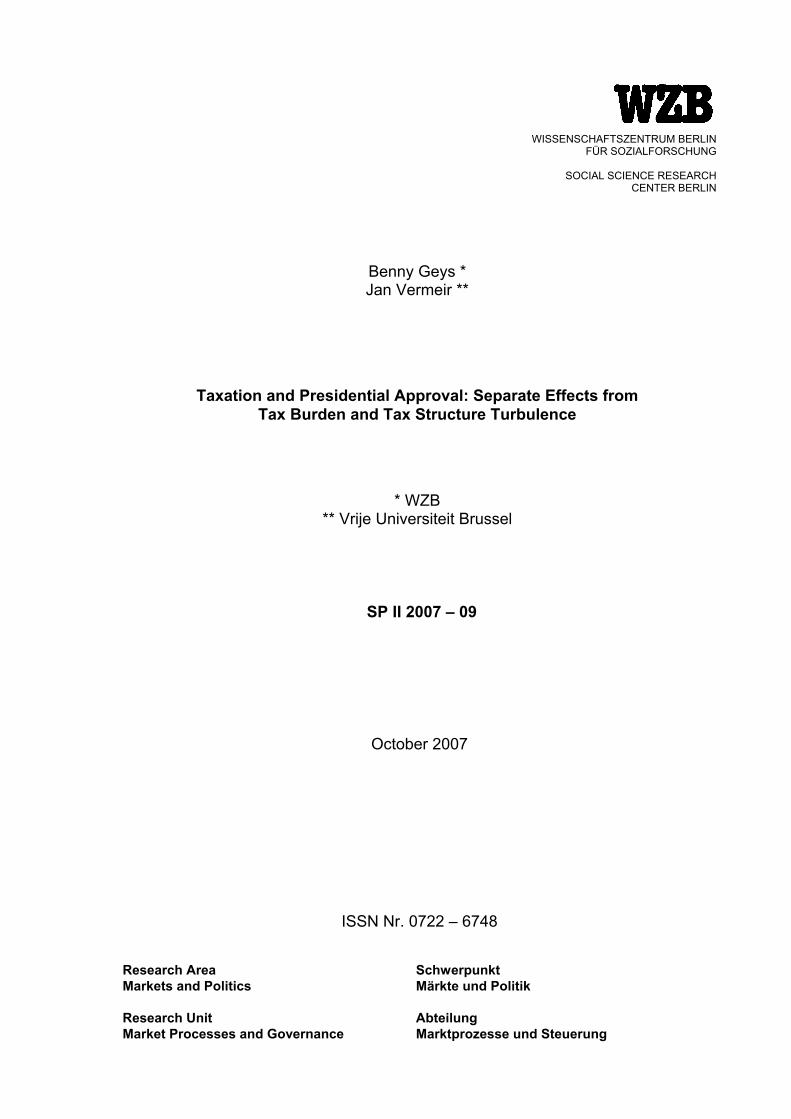
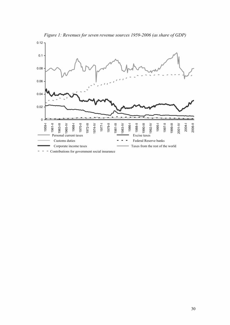
In Figure 1, we present quarterly data on US federal government revenues (as a share

of GDP). The data are seasonally adjusted using the US Census X-12 seasonal

adjustment procedure and run from 1959:1 up to 2006:3. They are from the National

Income and Product Accounts Tables (NIPA) provided by the Bureau of Economic

Analysis.5 We use NIPA data because these exist on a quarterly basis (as opposed to

OECD revenue data) and thus allow us to analyse the impact of tax variables on

quarterly presidential approval ratings. The seven lines in the figure display revenues

3 Relatedly, it has been shown that the introduction of new taxes is significantly less likely in election

years (Mikesell, 1978; Berry, 1988; Berry and Berry, 1992; 1994 and Ashworth et al., 2006). 4 One might here draw a parallel with the theory of irreversible investment under uncertainty (cfr.

Dixit, 1989; Dixit and Pindyck, 1994; Belke and Goecke, 1999; Rose, 2000) to explain inertia in government behaviour (and thus limited tax structure turbulence) prior to elections. That is, governments can be seen as investors in fiscal policy (which cannot be reversed without incurring additional costs). The outcome of their fiscal projects is a priori uncertain. Some of these projects are profitable in terms of popularity while others are not. Given this uncertainty, there is an incentive for the government to wait with changes in the tax structure (i.e. investing) until the uncertainty has resolved (i.e. after the election) (cfr. Dixit, 1989). Hence, there is an “option value” to waiting. We are grateful to an anonymous referee for pointing this out to us.

5 The data (NIPA Tables, Table 3.2.) are available from the year 1947, but in their current form they start in 1959.

8

from the seven main revenue categories distinguished in the NIPA-tables: personal

current taxes, excise taxes, customs duties, taxes on Federal Reserve banks, corporate

income taxes, taxes from the rest of the world (barely visible in Figure 1 due to their

small revenues as a share of GDP) and contributions for government social insurance.

These seven categories together make up more than 94% of total revenues in each

quarter over the period 1959-2006.

__________________

Figure 1

about here

__________________

Figure 1 shows that revenues from personal current taxes have been the major source

of tax revenues over most of the period, hovering around 8% of GDP. Revenues from

corporate income taxes and excise taxation have been growing at (much) slower pace

than GDP over the period, thus generating the downward sloping curve in Figure 1 for

these two revenue sources. Social insurance contributions as a share of GDP have on

the other hand been steadily increasing – though their growth has levelled of since the

early 1990’s. The three remaining sources of tax revenues have generated only

marginal contributions to total tax revenues and have remained relatively stable in

relation to GDP over the period. Overall, these various evolutions imply that

significant shifts have taken place in the US federal tax structure.

Following Hettich and Winer (1984, 1988) the tax structure can be thought of as the

shares of various taxes in total tax revenues. For example, in a situation with n taxes,

the tax structure can be represented as (R1,t, …, Rn,t), where Ri,t is the share of taxi in

9

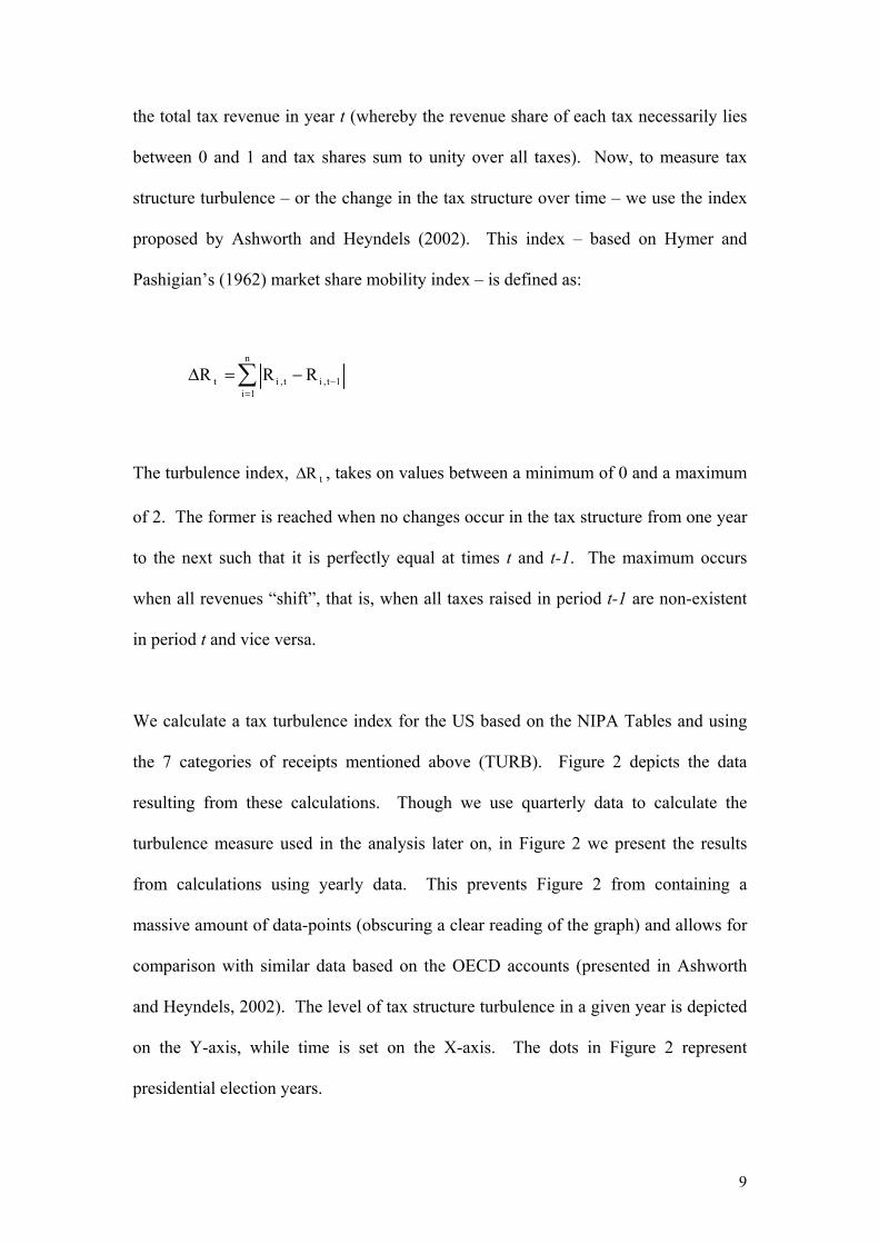
the total tax revenue in year t (whereby the revenue share of each tax necessarily lies

between 0 and 1 and tax shares sum to unity over all taxes). Now, to measure tax

structure turbulence – or the change in the tax structure over time – we use the index

proposed by Ashworth and Heyndels (2002). This index – based on Hymer and

Pashigian’s (1962) market share mobility index – is defined as:

∑=

−−=∆n

1i1t,it,it RRR

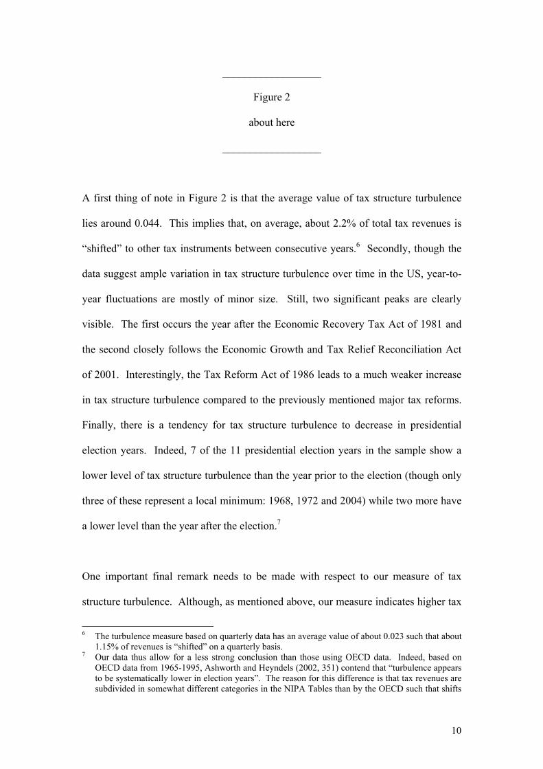
The turbulence index, tR∆ , takes on values between a minimum of 0 and a maximum

of 2. The former is reached when no changes occur in the tax structure from one year

to the next such that it is perfectly equal at times t and t-1. The maximum occurs

when all revenues “shift”, that is, when all taxes raised in period t-1 are non-existent

in period t and vice versa.

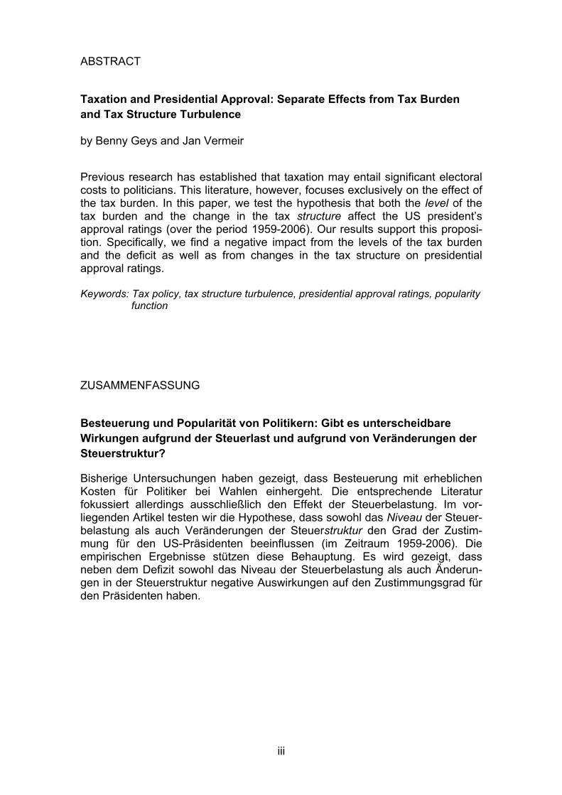
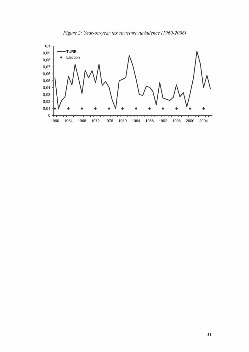
We calculate a tax turbulence index for the US based on the NIPA Tables and using

the 7 categories of receipts mentioned above (TURB). Figure 2 depicts the data

resulting from these calculations. Though we use quarterly data to calculate the

turbulence measure used in the analysis later on, in Figure 2 we present the results

from calculations using yearly data. This prevents Figure 2 from containing a

massive amount of data-points (obscuring a clear reading of the graph) and allows for

comparison with similar data based on the OECD accounts (presented in Ashworth

and Heyndels, 2002). The level of tax structure turbulence in a given year is depicted

on the Y-axis, while time is set on the X-axis. The dots in Figure 2 represent

presidential election years.

10

__________________

Figure 2

about here

__________________

A first thing of note in Figure 2 is that the average value of tax structure turbulence

lies around 0.044. This implies that, on average, about 2.2% of total tax revenues is

“shifted” to other tax instruments between consecutive years.6 Secondly, though the

data suggest ample variation in tax structure turbulence over time in the US, year-to-

year fluctuations are mostly of minor size. Still, two significant peaks are clearly

visible. The first occurs the year after the Economic Recovery Tax Act of 1981 and

the second closely follows the Economic Growth and Tax Relief Reconciliation Act

of 2001. Interestingly, the Tax Reform Act of 1986 leads to a much weaker increase

in tax structure turbulence compared to the previously mentioned major tax reforms.

Finally, there is a tendency for tax structure turbulence to decrease in presidential

election years. Indeed, 7 of the 11 presidential election years in the sample show a

lower level of tax structure turbulence than the year prior to the election (though only

three of these represent a local minimum: 1968, 1972 and 2004) while two more have

a lower level than the year after the election.7

One important final remark needs to be made with respect to our measure of tax

structure turbulence. Although, as mentioned above, our measure indicates higher tax

6 The turbulence measure based on quarterly data has an average value of about 0.023 such that about

1.15% of revenues is “shifted” on a quarterly basis. 7 Our data thus allow for a less strong conclusion than those using OECD data. Indeed, based on

OECD data from 1965-1995, Ashworth and Heyndels (2002, 351) contend that “turbulence appears to be systematically lower in election years”. The reason for this difference is that tax revenues are subdivided in somewhat different categories in the NIPA Tables than by the OECD such that shifts

11

structure turbulence in years with significant changes in the federal tax law (and thus

picks up the effect of significant policy changes), it is also likely to be influenced by

changes in economic conditions that affect government revenues levels and structures

(e.g. growth, inflation and so on). However, under the assumption that voters

understand the effect of economic variables on fiscal outcomes “they should penalize

incumbents only for that part of any tax change which is unanticipated, given

economic changes” (Besley and Case, 1995, 40). In that case, effects from economic

factors should be separated from those of discretionary tax policy changes.

Obviously, however, this assumption with respect to voters’ understanding of

economic conditions – and their effects on fiscal outcomes – may not be too credible.

We return to this issue in the following section.

4. Empirical Analysis

4.1. Empirical specification

To test whether there is a fixed cost to changing tax policies – irrespective of whether

the total tax burden is increased or decreased – we estimate a presidential popularity

function for the US over the period 1959:1-2006:3 including both the level of the tax

burden and the change in the tax structure. Specifically, our basic specification is:

Pt = a + bi Pt-i + b3 Xt + b4 DEFt + b5 REVt + b6 TURBt + et with i = 1, 2

between categories in the OECD data may not constitute a shift in the NIPA data, and vice versa. As mentioned, we prefer the use of the NIPA data as these allow for an analysis of quarterly data.

12

Where P represents US Presidential Popularity, X is a vector of control variables

(explained below), DEF refers to the US Federal Government budget deficit (as a %

of GDP), REV equals the total tax burden (as a % of GDP) and TURB is our measure

of tax structure turbulence.

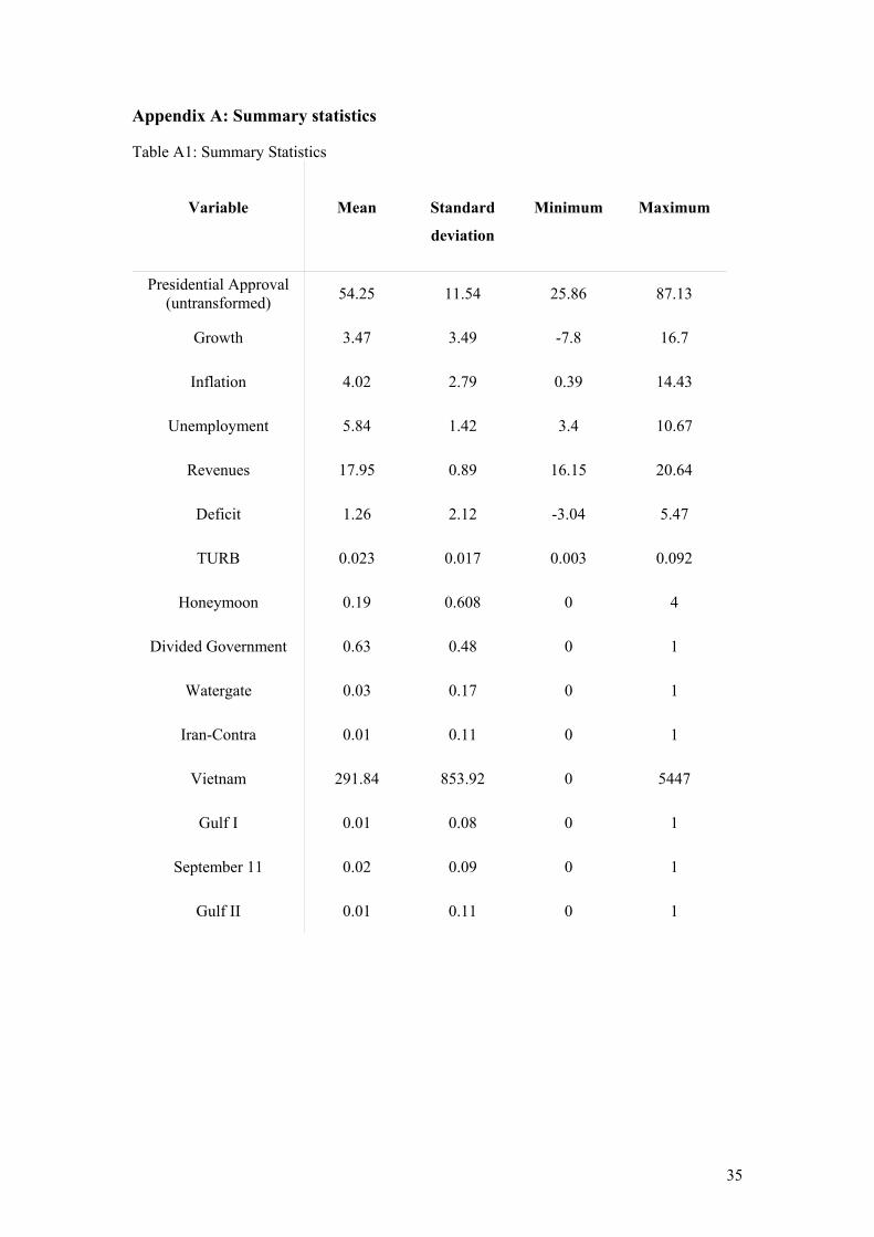
In line with Baum and Kernell (2001), the dependent variable of our model (Pt)

represents a logistic transformation of the US president’s popularity level in quarter t:

ln(APPt /(100 – APPt)), whereby APP is defined as the average Gallup approval rating

in that quarter (summary statistics for all variables are provided in Appendix A). We

apply this transformation as popularity is bounded between 0 and 100 (and

transforming the popularity ratings prevents estimated coefficients to lie outside this

allowable interval).

As explanatory variables, our model first of all includes lags of the dependent variable

Pt-i (with i = 1, 2). The number of lags (i.e. two) used in the final model is thereby

chosen such as to avoid problems of autocorrelation (cfr. Veiga and Veiga, 2004).

This occurs when two lags of the dependent variable are introduced.8 Xt is a vector

comprising a number of standard control variables (more extensively discussed later

on). Central to the analysis, however, are three fiscal variables. DEFt represents the

budget deficit, measured by the difference between current expenditures and current

revenues of the US federal government, as a percentage of GDP, in the current

quarter. This is included to test the hypothesis that voters are averse to budget deficits

(Niskanen, 1979; Peltzman, 1992; Kelleher and Wolak, 2005). As such, we expect b4

< 0. REVt is a measure for the total tax burden. It is operationalised as the sum of

8 When including only one lag of the dependent variable, the null hypothesis of no autocorrelation is

significantly rejected for all specifications.

13

current tax receipts and contributions for government social insurance, as a percentage

of GDP. In line with findings in previous empirical work, we expect a higher tax

burden to lower the president’s approval ratings such that b5 < 0. Finally, TURBt

measures the effect of tax structure turbulence on presidential approval ratings.

Following the arguments of Rose (1985) and Rose and Karran (1987), we expect this

index to have a negative effect on popularity, b6 < 0.9

Our vector of control variables, Xt, contains both economic and political controls. As

economic variables, we incorporate the real growth rate of GDP, the inflation rate and

the unemployment rate in the current quarter. While the former is expected to lead to

higher approval ratings, the latter two are expected to lower the president’s popularity.

As political variables, we first include a set of administration dummy variables (as is

customary in the literature). These assess the existence of any president-specific

effects on popularity ratings. Our second political variable assesses the existence of a

“honeymoon” effect. This relates to the period of goodwill that a president faces in

the first quarters of his presidency (Mueller, 1970). We measure this by including a

variable that is 3 in the second quarter of each administration, 2 in the third quarter, 1

in the fourth quarter and 0 in all other quarters (Smyth and Dua, 1989; Fox and

Phillips, 2003). Thirdly, we include a dichotomous variable that is 1 in case of

divided government, 0 otherwise. In quarters with divided government, it is less clear

which party should be held responsible for policy, which might benefit the president’s

9 An anonymous referee indicated that popularity may affect contemporaneous economic and fiscal

variables (i.c. growth, inflation, unemployment, deficit, revenues), leading to a reverse causality problem. However, although the president may react to low popularity ratings by initiating given policy measures, this is likely to take some time in leading to observable results in economic outcomes. Hence, the contemporaneous (causal) effect of popularity on economic and fiscal variables is likely to be weak and unproblematic for the interpretation of our results.

14

popularity (Nicholson et al., 2002). This argument is in line with the “clarity of

responsibility” hypothesis suggested by Powell and Whitten (1993).

Then, we account for the effects of wars fought by the US army. We control for the

effects of the Vietnam War through a variable measuring the number of US military

casualties in the period 1964-1975. Earlier studies show that Vietnam represented a

political cost for the US president (Gronke and Newman, 2003). Though war-

casualties are bad for presidential popularity, short wars may actually improve his

position as voters might adhere to the “united we stand, divided we fall” adagio and

be more supportive towards their president. This “rally around the flag” effect then

creates a boost to approval ratings (Mueller, 1970). The effect of the first Gulf war is

analysed through a dichotomous variable equal to 1 in the quarters 1990:3-1991:1 and

0 otherwise (Nickelsburg and Norpoth, 2000). The second Gulf war is controlled for

with a dummy that is 1 in the first two quarters of 2003 (official combat was declared

over by President George W. Bush on May 1st).10 We also control for the rally effect

after 9/11. This rally has been remarkably long and slowly decaying compared to

previous rallies (Gaines, 2002; Hetherington and Nelson, 2003). Therefore, instead of

including a dichotomous variable, we allow for the 9/11 effect by creating a variable

that is zero in the quarters prior to 2003:3, and 1/i starting from that quarter (with i =

1, 2, 3, …). In addition, we allow for the effects of scandals involving the president.

A dummy to control for the Watergate scandal is 1 in the quarters 1973:2-1974:2, and

10 We also analysed the effect of the number of US killed and wounded in action in the current Iraq

campaign. These data were retrieved from www.icasualties.org and are based on official statistics from the US Department of Defense. Interestingly, however, the number of casualties and wounded soldiers does not appear to have a statistically significant detrimental effect on President Bush’ popularity over the period studied (not reported). Most likely, this effect is already taken up in the 9/11 effect. Indeed, removing the slowly decaying 9/11 variable from the estimations leads to a strongly negative impact of Iraq war casualties on approval ratings.

15

zero otherwise. The effect of the Iran-Contra affair is captured with a dummy equal

to 1 in the quarters 1986:4-1987:1, and zero otherwise.11

Finally, (unreported) preliminary analyses showed that both approval ratings and tax

structure turbulence witness significant seasonal trends when regressing these

variables on three dummies for the different quarters of the year. Hence, it is

important to include such dummy variables also in our final regression equations.

Failing to do this could lead to spurious regression results (whereby seasonal trends in

popularity are mistakenly judged to derive from tax structure turbulence). Hence,

dummy variables equal to 1 in quarters 1, 2 and 3 (and 0 otherwise) were included in

the final regression model.

4.2. Results

As mentioned, we test the model using data on US presidential approval ratings from

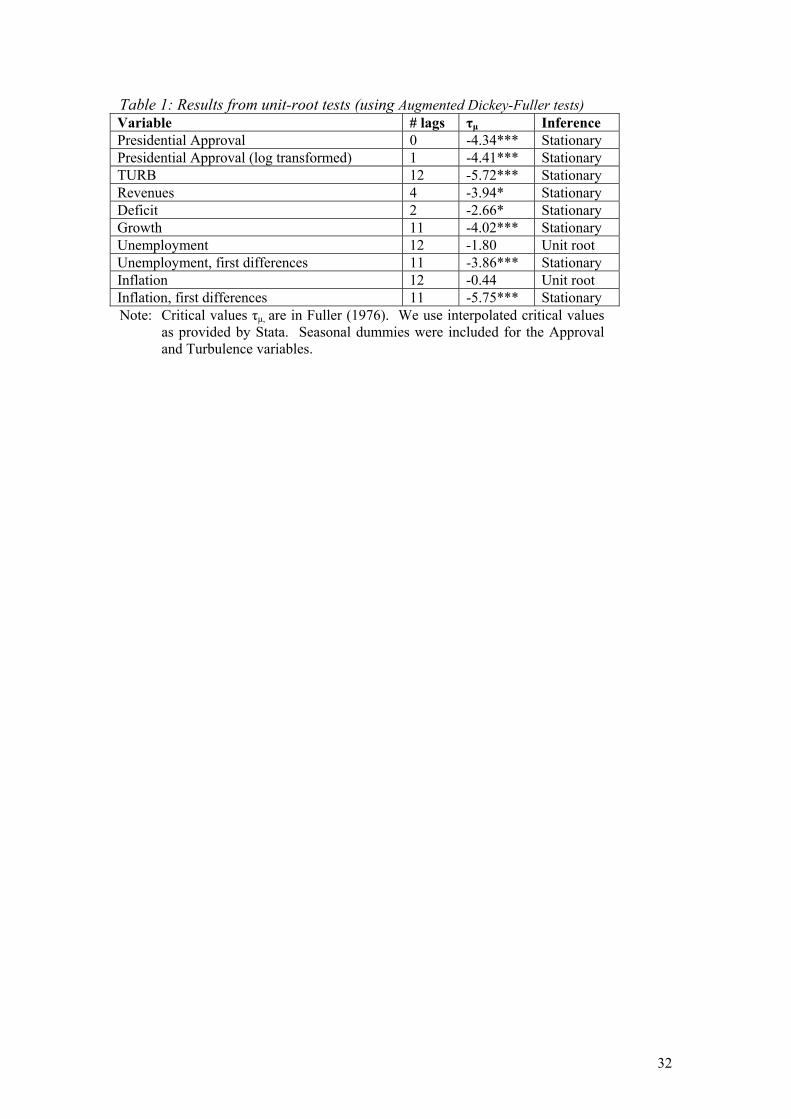
1959:3-2006:3.12 Still, before we turn to the estimation results, it is important to note

that unit root tests were performed to assess the stationarity of our variables. Failing

to test for this could lead to spurious inferences in time series analyses (Harris, 1995).

The results of the unit root tests (given in Table 1) indicate that all variables are

stationary, with the exception of unemployment and inflation. As first differences of

11 Interestingly, a dummy variable controlling for the (failed) impeachment procedure against

President Clinton following the Monica Lewinsky affair fails to reach statistical significance and is not retained in the final regression model. This corroborates Zaller’s (1998) finding that this affair did not harm Clinton’s popularity.

12 Two outliers were removed before estimation (i.e. second and third quarter of 1975). In these quarters tax structure turbulence was well above 0.10 whereas the average is only 0.023. We do not have an explanation for these outliers. We also drop the first observations of each administration, as we lack lags of the dependent variable for these quarters.

16

these variables are stationary, we include them in first-differenced form in our

regression model.13

__________________

Table 1

about here

__________________

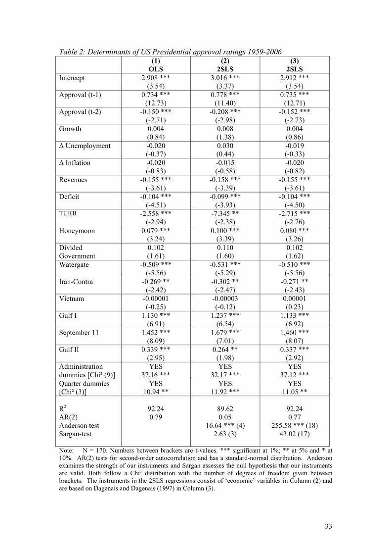
We present two sets of results. In Table 2, we assume that TURB accurately captures

tax structure turbulence. Hence, for the time being, we ignore the fact that part of the

movement in TURB might derive from changes in economic outcomes and their

effect on tax revenues (cfr. supra). We will explore this assumption further later on

(see Table 3). Column (1) in Table 2 presents results using simple OLS estimation,

presented mainly for reasons of comparison. In the remainder of the table, we instead

use 2SLS results to account for the fact that tax structure turbulence is likely to be

endogenous (see Ashworth and Heyndels, 2002). Given the difficulty to find

appropriate instruments, we thereby follow two different strategies. Column (2)

exploits a set of ‘economic’ instruments which have previously been shown to

influence tax structure turbulence in OECD countries (Ashworth and Heyndels,

2002): viz. a dummy variable indicating whether the quarter is in an election year or

not and the absolute value of the growth rate, the inflation rate and the unemployment

13 We perform augmented Dickey-Fuller regressions where the number of lagged first differences was

decided by a sequential general to specific rule (Hall, 1994; Maddala and Kim, 2004). This amounts to starting with a large number of lags (kmax) and to iteratively test the significance of the largest lag until one finds a significant one. Specifically, we follow Schwert (1989) to determine the starting lag length and set kmax = the integer part of [12 (T/100)1/4], with T representing the number of observations. Consequently, we use 13 lags as the point of departure (as T=183). When testing for a unit root in the turbulence and approval variables, we included quarterly dummies to control for seasonal effects (Enders, 2004). This was not necessary for the other economic and fiscal variables as these are seasonally adjusted data. Note also that a HEGY test for seasonal unit roots rejects the null hypothesis of unit root at zero, semi-annual and annual frequency for the approval and turbulence variables (Hylleberg et al., 1990) (results available upon request).

17

rate. Column (3) employs a set of ‘econometric’ instruments built based on third (and

higher) moments, as espoused by Dagenais and Dagenais (1997) and Lewbel (1997).14

These are by construction highly correlated with the turbulence measure, but are

uncorrelated with the dependent variable – making them intrinsically useful

instruments (though, unlike the ‘economic’ instruments, arguably harder to interpret

substantively). In each case, we provide the Anderson canonical correlation test and

the Sargan test for overidentifying restrictions to attest the appropriateness of the

instruments (see bottom rows of Table 2).

__________________

Table 2

about here

__________________

Before discussing the central – fiscal – variables of the model, we should note that all

three economic control variables perform poorly. None of them has a significant

effect on approval ratings. Growth and the change in unemployment are highly

correlated. When leaving out either of them, the effect of the other has the expected

sign and (at least approaches) statistical significance at conventional levels. The

political variables also confirm our expectations (and the results of the prior

literature). Particularly, we find clear evidence of president-specific effects, a highly

significant positive honeymoon effect, lower popularity ratings following the

14 These instruments involve demeaning the model’s explanatory variables. Denoting these demeaned

variables as x, the instruments used are a constant, z1 = x*x and z4 = x*x*x – 3x[E(x’x/N)*Ik] with * designating the Hadamard element by element matrix multiplication operator (see Dagenais and Dagenais, 1997, 197-198). This choice was dictated by the Monte Carlo simulations of Dagenais and Dagenais (1997) and involve the same terms as suggested by Lewbel (1997). Note that in the construction of these instruments, we exclude the lagged dependent variables as they are likely to be predetermined but not completely exogenous (and, as such, their internal correlation with the dependent variable may cause problems).

18

Watergate and Iran-Contra affairs and higher ratings in war-time as well as after 9/11

(in line with a “rally around the flag” effect; Mueller, 1970).

Turning our attention to the fiscal variables, the results provide support for the

negative impact of budget deficits on presidential popularity. This corroborates the

results of – among others – Niskanen (1979), Peltzman (1992) and Kelleher and

Wolak (2005) and indicates a desire for sound financial management and an aversion

to fiscal deficits in the electorate. Total government revenues as a share of GDP also

have the expected negative effect on US presidential popularity. This is in line with

the findings of Niskanen (1975; 1979), Peltzman (1992) and Cuzán and Bundrick

(1999). We should note at this point that a Wald test shows the coefficients for

revenues and deficit to be statistically distinct (Chi²(1) > 3.80 in all cases, p<0.10).

This result points out that voters dislike taxes slightly more than deferred taxation

(through deficit financing). That is, voters appear not to fully recognize that, given

the current value of future spending, “a deficit-financed cut in current taxes leads to

higher future taxes that have the same present value as the initial cut” (Barro, 1989,

38). Hence, against the basic tenet of the Ricardian Equivalence Theorem (which

states that a rearrangement of the timing of taxes has no first-order effect on aggregate

demand, and thereby on economic growth), shifting taxes into the future through

deficit financing has a small direct positive effect on government popularity.

Importantly, tax structure turbulence has the anticipated negative effect on

presidential popularity and this effect is statistically significant in the OLS regression

and when using the various sets of instruments. This finding thus is robust over all

specifications. This supports the contention that shifts in the tax structure impose a

19

political cost for the incumbent, even when these changes are revenue-neutral (cfr.

Rose, 1985; Rose and Karran, 1987). As a corollary to this finding, we can conclude

that politicians’ reduction of tax structure turbulence in election years (see Ashworth

and Heyndels, 2002) represents a rational response to these costs.15

Now we know that there is an independent effect of tax structure turbulence, we might

be interested in assessing the size of the estimated effects of our fiscal variables. The

coefficients in Table 2 are, however, not readily interpretable since the dependent

variable has been transformed (see above). Still, we can calculate the marginal effects

on the untransformed dependent variable as: (100 β exp(βx))/(1+exp(βx))², where β is

the coefficient in Table 2. As x we take the sample mean of the explanatory variable.

Using the results in column (3), we find that an increase in revenues (as a percentage

of GDP) with one percentage point lowers presidential approval with approximately

0.85 %. An increase in the deficit with one percentage point lowers approval with

2.57 %. Finally, an increase in tax structure turbulence with one standard deviation

(0.017) decreases approval with around 1.18 % (using the results in Column (3)).

These effects are clearly non-negligible.16

15 As the tax structure turbulence index has seven distinct components, it is interesting to see whether

all components have the same impact on popularity. Including the revenues from the different types of taxation directly into the VP-function, we find that the strongest negative effects of taxation on popularity derive from social security contributions and excise tax revenues. Given that the major component of the excise program is motor fuel, this suggests that the US public is very sensitive to taxes on its mobility and wage income. Income and corporate taxation also significantly depress presidential popularity. Interestingly, tax revenues from the ‘rest of the world’ have a small positive effect (which is only significant at the 15% significance level).

16 The model estimated thus far is essentially a short-term model. To estimate possible long-term effects, we included both the difference (to assess short-term effects) and lags (to assess long-term effects) of our economic and fiscal variables. These additional results (available upon request) indicate that the long- and short-term effects of growth and inflation are roughly similar in size (with growth having a positive and mostly significant effect and inflation an insignificant one). Unemployment appears to have a positive short-term effect and a negative long-term effect (though both are statistically insignificant). Both revenues and the deficit have significant negative long-term effects (while short-term effects are insignificant). Finally, the effect of tax structure turbulence is negative in both short- and long-term perspective, though statistical significance is generally stronger for the short-term coefficient. Hence, tax structure turbulence affects

20

Up to this point, we have (implicitly) assumed that our tax structure turbulence

variable accurately reflects policy initiatives. However, as mentioned before,

although TURB indicates higher tax structure turbulence in years with significant

changes in the federal tax law (and thus picks up the effect of important policy

changes - see section 3), it is likely to be also influenced by changes in economic

conditions that affect government revenues (e.g. growth, inflation and so on). The

same obviously might also hold for the other two other fiscal variables in the model.

The results in Table 2 do not allow a clear conclusion as to whether the observed

effect of tax structure turbulence (nor of the revenues and deficit) on presidential

popularity is due to the effect of discretionary policy decisions or effects from the

economy. Consequently, one might argue that these ‘economic’ effects should be

separated from those of discretionary tax policy changes. While this argument has

some theoretical merit, we feel that it is empirically less satisfactory for two reasons.

Firstly, it entails the assumption that voters understand the effect of economic

variables on fiscal outcomes and (are able to) perform regression-based evaluations of

politicians to distinguish between both effects. This appears, at best, implausible (for

a similar argument, see Besley and Case, 1995, 40). Moreover, voters may simply

want to punish unfavourable fiscal outcomes independent of their cause (be it the

economy or tax reform).

Nevertheless, following Besley and Case (1995), we test whether voters do in reality

make a difference between variations in fiscal outcomes caused by discretionary

policy decisions from those generated by the economy (a related idea is exploited in

presidential popularity, but mainly appears to do so in the short-term (which supports the contention that it is to be avoided when elections are imminent). We are grateful to a referee for suggesting

21

Bordignon et al., 2003; Allers and Elhorst, 2005). Specifically, we estimate three

auxiliary regressions with our three fiscal variables as the respective dependent

variables and GDP growth, inflation and unemployment as explanatory variables.17

Importantly, the predicted values of these auxiliary regressions are the fiscal outcomes

as they are anticipated given the economic conditions in that quarter (Besley and

Case, 1995). The error terms, however, indicate the effect of discretionary policy

changes on the three fiscal variables. These effects may be termed ‘unanticipated’ –

reflecting that they are not expected given changes in economic conditions. By

including both the predicted values and the errors from these auxiliary regressions in a

model explaining US presidential popularity, we would expect that only the latter lead

to electoral punishment. The reason is that (rational) voters should not punish

incumbents for changes in fiscal outcomes caused by economic forces (as such effects

would be ‘anticipated’), but should reserve punishment for effects caused by

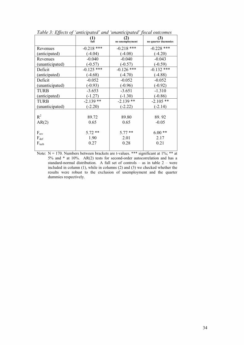
discretionary changes in tax policies. The results are presented in Table 3 (as the

results for the control variables mirror those in Table 2, we suppress their results here

for space reasons). Column (1) presents results for the baseline model (using all

control variables as presented in Table 2), while columns (2) and (3) report on

robustness checks in which we excluded unemployment (given its correlation with

GDP growth) and the quarterly dummies, respectively, from the model.

____________________

Table 3

about here

this extension to our model.

17 In the regression for tax structure turbulence, we use the absolute value of the changes in the three explanatory variables (as variations in any direction are likely to have the same effect on tax structure turbulence, where this is clearly not the case for fiscal revenue and deficit levels). Also, in all first stage regressions, we include a lagged dependent variable to correct for first-order autocorrelation and quarterly dummies to account for seasonal effects.

22

____________________

The findings in Table 3 look somewhat counter-intuitive at first sight. Indeed, we

find that presidential popularity is significantly negatively affected by anticipated

increases in total tax revenues and deficits, but not by unanticipated increases. On the

other hand, approval is significantly negatively affected by unanticipated changes in

tax structure turbulence, but not by anticipated changes. Taking these results at face

value would imply that voters respond to changes in tax revenues and deficit caused

by the economy only (which are changes they should ‘anticipate’) whereas they only

react to tax structure turbulence if it is generated by discretionary policy changes.

Still, F-tests – reported at the bottom of Table 3 – indicate that the difference between

‘anticipated’ and ‘unanticipated’ effects is statistically significant only for revenues

(at the 95% confidence level). Hence, to the limited extent that voters do distinguish

between these two sources of variation, it does not appear to lead to consistent

reactions (since they appear to react to ‘anticipated’ revenues and deficits, but to

‘unanticipated’ turbulence). Interestingly, while Besley and Case (1995, 40) find that

voters react to ‘unanticipated’ changes in income tax liabilities (in line with rational

behavior), they nonetheless remain sceptical as to the “plausibility of assuming that

voters are doing regression-based evaluations of incumbents in their heads”. So are

we. Hence, the overall inference to be drawn from these results appears to be that

voters do not effectively distinguish between variations in fiscal outcomes caused by

the economy or the incumbent’s discretionary policy decisions.

23

5. Conclusion

The literature on VP-functions shows that taxation has an important effect on the

popularity and re-election odds of politicians. However, these earlier studies on the

electoral cost of taxation have concentrated on the effect of changes in overall tax

burden and disregarded potential effects from changes in the tax structure. Still, as

argued by Rose (1985) and Rose and Karran (1987), an incumbent’s popularity is

likely to be maximised, ceteris paribus, under a stable and unchanging tax system.

The argument builds on the notion that tax changes have (fixed) costs irrespective of

whether taxes are increased or lowered. Following this line of argument, in the

present paper we have tested the impact of both the total tax burden and tax structure

changes on US presidential popularity.

Our data consist of quarterly approval ratings for the incumbent US president over the

period 1959-2004. As a measure for the change in the tax system, we use a tax

structure turbulence index similar to the one used by Ashworth and Heyndels (2002).

The results indicate that fiscal policy has an important influence on presidential

approval ratings. Specifically, we find that approval ratings suffer from both

increases in the tax burden and the deficit. In line with the theoretical predictions by

Rose (1985) and Rose and Karran (1987), tax structure turbulence has a negative

effect on presidential approval. Hence, politicians act rationally in trying to avoid this

cost of taxation by minimizing tax structure turbulence when elections are imminent

(as found by Ashworth and Heyndels, 2002).

24

References

Allers, M.A. & Elhorst J.P. (2005), Tax mimicking and yardstick competition among

local governments in the Netherlands. International Tax and Public Finance,

12(4), 493-513.

Ashworth, J. & Heyndels, B. (2000). Politicians’ opinions on tax reform. Public

Choice, 103, 117-138.

Ashworth, J. & Heyndels, B. (2002). Tax structure turbulence in OECD countries.

Public Choice, 111, 347-376.

Ashworth, J., Geys, B., & Heyndels, B. (2006). Determinants of tax innovation: The

case of environmental taxes in Flemish municipalities. European Journal of

Political Economy, 22(1), 223-247.

Barro, R.J. (1989). The Ricardian approach to budget deficits. Journal of Economic

Perspectives, 3(2), 37-54.

Baum, M.A. & Kernell, S. (2001). Economic class and popular support for Franklin

Roosevelt in war and peace. Public Opinion Quarterly, 65, 198-229.

Belke, A. & Goecke, M. (1999). A Simple Model of Hysteresis in Employment under

Exchange Rate Uncertainty. Scottish Journal of Political Economy, 46, 260-286.

Berry, F.S. (1988). Tax policy innovation in the American states. (Ann Arbor,

Michigan: UMI Dissertation Services).

Berry, F.S. & Berry, W.D. (1992). Tax innovation in the States: Capitalizing on

political opportunity. American Journal of Political Science, 36(3), 715-742.

Berry, F.S. & Berry, W.D. (1994). The politics of tax increases in the States.

American Journal of Political Science, 38(3), 855-859.

Besley, T. & Case, A. (1995). Incumbent behavior: Vote-seeking, tax-setting and

yardstick competition. American Economic Review, 85, 25-45.

Bloom, H.S. & Price, H.D. (1975). Voter response to short-run economic conditions:

The asymmetric effect of prosperity and recession. American Political Science

Review 69(4), 1240-1254.

25

Bordignon, M., Cerniglia, F. & Revelli, F. (2003). In search of yardstick competition:

a spatial analysis of Italian municipality property tax setting. Journal of Urban

Economics, 54, 199-217.

Case, A. (1994). Taxes and the electoral cycle: How sensitive are governors to

coming elections? Business Review, March/April, 17-26.

Cusack, T.R. (1999). The shaping of popular satisfaction with government and regime

performance in Germany. British Journal of Political Science, 29, 641-72.

Cuzán, A.G. & Bundrick, C.M. (1999). Fiscal policy as a forecasting factor in

Presidential elections. American Politics Quarterly, 27(3), 338-353.

Dagenais, M.G. & Dagenais, D.L., (1997). Higher moment estimators for linear

regression modes with errors in variables. Journal of Econometrics, 76, 193-221.

Dixit, A. (1989). Entry and Exit Decisions under Uncertainty. Journal of Political

Economy, 97, 620-638.

Dixit, A. & Pindyck, R. (1994). Investment under uncertainty. (Princeton: Princeton

University Press.)

Eismeier, T.J. (1979). Budgets and ballots: The political consequences of fiscal

choice. (In D. Rae & T. Eismeier (Eds.), Public Policy and Public Choice (pp. 121-

149). Beverly Hills: Sage.)

Enders, W. (2004). Applied econometric time series (2nd edition). (Hoboken, NJ: John

Wiley and Sons Ltd.)

Fox, G. & Phillips, E.N. (2003). Interrelationship between presidential approval,

presidential votes and macroeconomic performance, 1948-2000. Journal of

Macroeconomics, 25, 411-424.

Fuller, W.A. (1976). Introduction to statistical time-series. (New York: John Wiley

and Sons.)

Gaines, B.J. (2002). Where’s the rally? Approval and trust of the president, cabinet,

congress, and government since September 11. PS: Political Science and Politics,

35(3), 531-536.

26

Geys, B. & Vermeir, J. (2007). The political cost of taxation: New evidence from

German popularity ratings. Paper presented at the annual meeting of the Verein für

Sozialpolitik, September 2007, München.

Gibson, J.G. (1994). Voter reaction to tax change: the case of the poll tax. Applied

Economics, 26, 877-884.

Gronke, P. & Newman, B. (2003). FDR to Clinton, Mueller to ?: A field essay on

presidential approval. Political Research Quarterly, 56(4), 501-512.

Hall, A. (1994). Testing for a unit root in time series with pretest data-based model

selection. Journal of Business and Economic Statistics, 12, 461-470.

Hansen, S.B. (1999). Life is not fair: Governors’ job performance ratings and state

economies. Political Research Quarterly, 52, 167-188.

Happy, J.R. (1992). The effect of economic and fiscal performance on incumbency

voting: The Canadian case. British Journal of Political Science, 22, 117-130.

Harris, R.I.D. (1995). Using cointegration analysis in econometric modelling.

(Harlow: Pearson Education.)

Hausman, J. (1978). Specification tests in econometrics. Econometrica, 46(6), 1251-

1271.

Hetherington, M.J. & Nelson, M. (2003). Anatomy of a rally effect: George W. Bush

and the war on terrorism. PS: Political Science and Politics, 36(1), 37-42.

Hettich, W. & Winer, S.L. (1984). A positive model of tax structure. Journal of

Public Economics, 24, 67-87.

Hettich, W. & Winer, S.L. (1988). Economic and political foundations of tax

structure. American Economic Review, 78, 701-712.

Hibbs, D.A., Jr. (2000). Bread and peace voting in U.S. presidential elections. Public

Choice, 104, 149-180.

Hibbs, D.A., Jr. & Madsen, H.J. (1981). The impact of economic performance on

electoral support in Sweden, 1967-1978. Scandinavian Political Studies, 4, 33-50.

Hylleberg, S., Engle, R., Granger, C. & Yoo, B. (1990). Seasonal integration and

cointegration. Journal of Econometrics, 44, 215-238.

27

Hymer, S. & Pashigian, P. (1962). Turnover of firms as a measure of market

behaviour. Review of Economics and Statistics, 44, 82-87.

Johnston, P., Lynch, F. & Walker, J.G. (2005). Income taxes and elections in Britain,

1950-2001. Electoral Studies, 24(3), 393-408.

Kahneman, D. & Tversky, A. (1979). Prospect theory: An analysis of decision under

risk. Econometrica, 47(2), 263-291.

Kelleher, C.A. & Wolak, J. (2005, April). Citizen confidence in State government

institutions. (Paper presented at the MPSA National Conference, Chicago).

Kone, S.L. & Winters, R.F. (1993). Taxes and voting: Electoral retribution in the

American states. Journal of Politics, 55, 22-40.

Landon, S. & Ryan, D.L. (1997). The political costs of taxes and government

spending. Canadian Journal of Economics, 30, 85-111.

Lewbel, A. (1997). Constructing instruments for regressions with measurement error

when no additional data are available, with an application to patents and R&D.

Econometrica, 65, 1201-1213.

Lowry, R.C., Alt, J.E. & Ferree, K.E. (1998). Fiscal policy outcomes and electoral

accountability in American states. American Political Science Review, 92, 759-

774.

MacDonald, J.A. & Sigelman, L. (1999). Public assessments of gubernatorial

performance. A comparative state analysis. American Politics Quarterly, 27, 201-

215.

Maddala, G.S. & Kim, I.M. (2004). Unit roots, cointegration and structural change.

(Cambridge: Cambridge University Press.)

McCaffery, E.J. & Baron, J. (2004), Thinking about Tax, Center for the Study of Law

and Politics working paper nr. 33, California Institute of Technology.

Mikesell, J.L. (1978). Election periods and state tax policy cycles. Public Choice, 33,

99-105.

Mueller, J. (1970). Presidential popularity from Truman to Johnson. American

Political Science Review, 64, 18-34.

28

Nannestad, P. & Paldam, M. (1994). The VP-function: A survey of the literature on

vote and popularity functions after 25 years. Public Choice, 79, 213-245.

Nannestad, P. & Paldam, M. (1997). The grievance asymmetry revisited: A micro

study of economic voting in Denmark, 1986-92. European Journal of Political

Economy 13, 81-99.

Nickelsburg, M. & Norpoth, H. (2000). Commander-in-chief or chief economist? The

president in the eye of the public. Electoral Studies, 19, 313-332.

Nicholson, S.P., Segura, G.M. & Woods, N.D. (2002). Presidential approval and the

mixed blessing of divided government. Journal of Politics, 64(4), 701-720.

Niemi, R.G., Stanley, H.W. & Vogel, R.J. (1995). State economies and state taxes: Do

voters hold governors accountable? American Journal of Political Science, 39,

936-957.

Niskanen, W.A. (1975). Bureaucrats and politicians. 1975. Journal of Law and

Economics, 18, 617-643.

Niskanen, W.A. (1979). Economic and fiscal effects on the popular vote for the

president. (In D. Rae & T. Eismeier (Eds.), Public Policy and Public Choice (pp.

93-120). Beverly Hills: Sage.)

Paldam, M. & Schneider, F. (1980). The macro-economic aspects of government and

opposition popularity in Denmark 1957-78. Nationalokonomisk Tidsskrift, 2, 149-

170.

Peltzman, S. (1992). Voters as fiscal conservatives. Quarterly Journal of Economics,

107, 327-361.

Peters, B.G. (1991). The politics of taxation. (Cambridge: Basil Blackwell.)

Pissarides, C.A. (1980). British government popularity and economic performance.

The Economic Journal, 90, 569-581.

Pomper, G.M. (1968). Elections in America: Control and influence in American

politics. (New York: Dodd, Mead & Company.)

Powell, G.B. & Whitten, G.D. (1993). A cross-national analysis of economic voting:

Taking account of the political context. American Journal of Political Science, 37,

391-414.

29

Rose, R. (1985). Maximizing tax revenue while minimizing political costs. Journal of

Public Policy, 5, 289-320.

Rose, C. (2000). The I-R Hump: Irreversible Investment under Uncertainty. Oxford

Economic Papers, 52, 626-636.

Rose, R. & Karran, T. (1987). Taxation by political inertia. (London: Allen & Unwin)

Schwert, G.W. (1989). Test for unit roots: A Monte Carlo investigation. Journal of

Business and Economics Statistics, 7, 147-159.

Smyth, D.J. & Dua, P. (1989). The public’s indifference map between inflation and

unemployment: Empirical evidence for the Nixon, Ford, Carter and Reagan

presidencies. Public Choice, 60, 71-85.

Sobel, R.S. (1998). The political costs of tax increases and expenditure reductions:

Evidence from state legislative turnover. Public Choice, 96, 61-79.

Stults, B.G. & Winters, R.F. (2005). The political economy of taxes and the vote.

Unpublished Manuscript.

Turett, S. (1971). The vulnerability of American governors, 1900-1969. Midwest

Journal of Political Science, 15, 108-132.

Tversky, A. & Kahneman, D. (1991). Loss aversion in risk-less choice: A reference-

dependent model. Quarterly Journal of Economics 106(4), 1039-1061.

Veiga, F.J. & Veiga, L.G. (2004). The determinants of vote intentions in Portugal.

Public Choice, 118, 341-364.

Zaller, J. (1998). Monica Lewinsky's contribution to political science. PS: Political

Science and Politics, 31, 182-189.

30

Figure 1: Revenues for seven revenue sources 1959-2006 (as share of GDP)

0

0.02

0.04

0.06

0.08

0.1

0.12 1

959-

I

196

1-II

196

3-III

196

5-IV

196

8-I

197

0-II

197

2-III

197

4-IV

197

7-I

197

9-II

198

1-III

198

3-IV

198

6-I

198

8-II

199

0-III

199

2-IV

199

5-I

199

7-II

199

9-III

200

1-IV

200

4-I

200

6-II

Personal current taxes Excise taxes Customs duties Federal Reserve banks Corporate income taxes Taxes from the rest of the worldContributions for government social insurance

31

Figure 2: Year-on-year tax structure turbulence (1960-2006)

0

0,01

0,02

0,03

0,04

0,05

0,06

0,07

0,08

0,09

0,1

1960 1964 1968 1972 1976 1980 1984 1988 1992 1996 2000 2004

TURBElection

32

Table 1: Results from unit-root tests (using Augmented Dickey-Fuller tests) Variable # lags τµ Inference Presidential Approval 0 -4.34*** Stationary Presidential Approval (log transformed) 1 -4.41*** Stationary TURB 12 -5.72*** Stationary Revenues 4 -3.94* Stationary Deficit 2 -2.66* Stationary Growth 11 -4.02*** Stationary Unemployment 12 -1.80 Unit root Unemployment, first differences 11 -3.86*** Stationary Inflation 12 -0.44 Unit root Inflation, first differences 11 -5.75*** Stationary Note: Critical values τµ, are in Fuller (1976). We use interpolated critical values

as provided by Stata. Seasonal dummies were included for the Approval and Turbulence variables.

33

Table 2: Determinants of US Presidential approval ratings 1959-2006 (1)

OLS (2)

2SLS (3)

2SLS Intercept 2.908 ***

(3.54) 3.016 ***

(3.37) 2.912 ***

(3.54) Approval (t-1) 0.734 ***

(12.73) 0.778 ***

(11.40) 0.735 ***

(12.71) Approval (t-2)

-0.150 *** (-2.71)

-0.208 *** (-2.98)

-0.152 *** (-2.73)

Growth 0.004 (0.84)

0.008 (1.38)

0.004 (0.86)

∆ Unemployment -0.020 (-0.37)

0.030 (0.44)

-0.019 (-0.33)

∆ Inflation -0.020 (-0.83)

-0.015 (-0.58)

-0.020 (-0.82)

Revenues -0.155 *** (-3.61)

-0.158 *** (-3.39)

-0.155 *** (-3.61)

Deficit -0.104 *** (-4.51)

-0.099 *** (-3.93)

-0.104 *** (-4.50)

TURB -2.558 *** (-2.94)

-7.345 ** (-2.38)

-2.715 *** (-2.76)

Honeymoon 0.079 *** (3.24)

0.100 *** (3.39)

0.080 *** (3.26)

Divided Government

0.102 (1.61)

0.110 (1.60)

0.102 (1.62)

Watergate -0.509 *** (-5.56)

-0.531 *** (-5.29)

-0.510 *** (-5.56)

Iran-Contra -0.269 ** (-2.42)

-0.302 ** (-2.47)

-0.271 ** (-2.43)

Vietnam -0.00001 (-0.25)

-0.00003 (-0.12)

0.00001 (0.23)

Gulf I 1.130 *** (6.91)

1.237 *** (6.54)

1.133 *** (6.92)

September 11 1.452 *** (8.09)

1.679 *** (7.01)

1.460 *** (8.07)

Gulf II 0.339 *** (2.95)

0.264 ** (1.98)

0.337 *** (2.92)

Administration dummies [Chi² (9)]

YES 37.16 ***

YES 32.17 ***

YES 37.12 ***

Quarter dummies [Chi² (3)]

YES 10.94 **

YES 11.92 ***

YES 11.05 **

R2

AR(2) Anderson test Sargan-test

92.24 0.79

89.62 0.05

16.64 *** (4) 2.63 (3)

92.24 0.77

255.58 *** (18) 43.02 (17)

Note: N = 170. Numbers between brackets are t-values. *** significant at 1%; ** at 5% and * at 10%. AR(2) tests for second-order autocorrelation and has a standard-normal distribution. Anderson examines the strength of our instruments and Sargan assesses the null hypothesis that our instruments are valid. Both follow a Chi² distribution with the number of degrees of freedom given between brackets. The instruments in the 2SLS regressions consist of ‘economic’ variables in Column (2) and are based on Dagenais and Dagenais (1997) in Column (3).

34

Table 3: Effects of ‘anticipated’ and ‘unanticipated’ fiscal outcomes (1)

full (2)

no unemployment (3)

no quarter duzmmies Revenues (anticipated)

-0.218 *** (-4.04)

-0.218 *** (-4.08)

-0.228 *** (-4.20)

Revenues (unanticipated)

-0.040 (-0.57)

-0.040 (-0.57)

-0.043 (-0.59)

Deficit (anticipated)

-0.125 *** (-4.68)

-0.126 *** (-4.70)

-0.132 *** (-4.88)

Deficit (unanticipated)

-0.052 (-0.93)

-0.052 (-0.96)

-0.052 (-0.92)

TURB (anticipated)

-3.653 (-1.27)

-3.651 (-1.30)

-1.310 (-0.86)

TURB (unanticipated)

-2.139 ** (-2.20)

-2.139 ** (-2.22)

-2.105 ** (-2.14)

R2

AR(2) Frev Fdef Fturb

89.72 0.65

5.72 **

1.90 0.27

89.80 0.65

5.77 **

2.01 0.28

89. 92 -0.05

6.00 **

2.17 0.21

Note: N = 170. Numbers between brackets are t-values. *** significant at 1%; ** at 5% and * at 10%. AR(2) tests for second-order autocorrelation and has a standard-normal distribution. A full set of controls – as in table 2 – were included in column (1), while in columns (2) and (3) we checked whether the results were robust to the exclusion of unemployment and the quarter dummies respectively.

35

Appendix A: Summary statistics Table A1: Summary Statistics

Variable

Mean

Standard

deviation

Minimum

Maximum

Presidential Approval (untransformed) 54.25 11.54 25.86 87.13

Growth 3.47 3.49 -7.8 16.7

Inflation 4.02 2.79 0.39 14.43

Unemployment 5.84 1.42 3.4 10.67

Revenues 17.95 0.89 16.15 20.64

Deficit 1.26 2.12 -3.04 5.47

TURB 0.023 0.017 0.003 0.092

Honeymoon 0.19 0.608 0 4

Divided Government 0.63 0.48 0 1

Watergate 0.03 0.17 0 1

Iran-Contra 0.01 0.11 0 1

Vietnam 291.84 853.92 0 5447

Gulf I 0.01 0.08 0 1

September 11 0.02 0.09 0 1

Gulf II 0.01 0.11 0 1

36

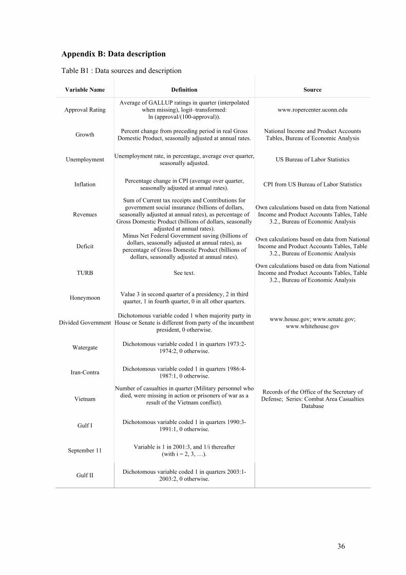
Appendix B: Data description Table B1 : Data sources and description

Variable Name

Definition

Source

Approval Rating Average of GALLUP ratings in quarter (interpolated

when missing), logit–transformed: ln (approval/(100-approval)).

www.ropercenter.uconn.edu

Growth Percent change from preceding period in real Gross Domestic Product, seasonally adjusted at annual rates.

National Income and Product Accounts Tables, Bureau of Economic Analysis

Unemployment Unemployment rate, in percentage, average over quarter, seasonally adjusted. US Bureau of Labor Statistics

Inflation Percentage change in CPI (average over quarter, seasonally adjusted at annual rates). CPI from US Bureau of Labor Statistics

Revenues

Sum of Current tax receipts and Contributions for government social insurance (billions of dollars,

seasonally adjusted at annual rates), as percentage of Gross Domestic Product (billions of dollars, seasonally

adjusted at annual rates).

Own calculations based on data from National Income and Product Accounts Tables, Table

3.2., Bureau of Economic Analysis

Deficit

Minus Net Federal Government saving (billions of dollars, seasonally adjusted at annual rates), as

percentage of Gross Domestic Product (billions of dollars, seasonally adjusted at annual rates).

Own calculations based on data from National Income and Product Accounts Tables, Table

3.2., Bureau of Economic Analysis

TURB See text. Own calculations based on data from National Income and Product Accounts Tables, Table

3.2., Bureau of Economic Analysis

Honeymoon Value 3 in second quarter of a presidency, 2 in third quarter, 1 in fourth quarter, 0 in all other quarters.

Divided Government Dichotomous variable coded 1 when majority party in

House or Senate is different from party of the incumbent president, 0 otherwise.

www.house.gov; www.senate.gov; www.whitehouse.gov

Watergate Dichotomous variable coded 1 in quarters 1973:2-1974:2, 0 otherwise.

Iran-Contra Dichotomous variable coded 1 in quarters 1986:4-1987:1, 0 otherwise.

Vietnam

Number of casualties in quarter (Military personnel who died, were missing in action or prisoners of war as a

result of the Vietnam conflict).

Records of the Office of the Secretary of Defense; Series: Combat Area Casualties

Database

Gulf I Dichotomous variable coded 1 in quarters 1990:3-1991:1, 0 otherwise.

September 11 Variable is 1 in 2001:3, and 1/i thereafter (with i = 2, 3, …).

Gulf II Dichotomous variable coded 1 in quarters 2003:1-2003:2, 0 otherwise.