1 Getting Started with the NI LabVIEW Digital Filter Design Toolkit

This tutorial provides several step-by-step exercises that introduce you to the NI LabVIEW Digital Filter Design Toolkit. These exercises teach you how to use the Digital Filter Design Toolkit within the LabVIEW graphical development environment and how you can design, analyze, and implement digital filters. After completing the tutorial, you will be able to design and analyze several types of digital filters.

This tutorial does not provide a comprehensive discussion of digital filter design. The information in the following exercises is limited to the specifics of the design at hand. Refer to the References section at the end of this document for a list of references that provide information about the theory and design of digital filters. Refer to the LabVIEW Digital Filter Design Toolkit User Manual for information about the digital filter design process and how to use the Digital Filter Design Toolkit VIs to design floating-point and fixed-point digital filters.

This tutorial does not provide an extensive introduction to the LabVIEW graphical development environment. If you are familiar with LabVIEW, you can work through these exercises to learn more about the Digital Filter Design Toolkit. For an overview of LabVIEW, refer to the related tutorial Getting Started with LabVIEW Virtual Instruments. You can access the Getting Started with LabVIEW Virtual Instruments tutorial by clicking the Start Tutorial Now button after you launch the LabVIEW 7.1 Online Evaluation version.

This tutorial only provides an introduction to the Digital Filter Design Toolkit. After you finish this tutorial, you can explore the Digital Filter Design Toolkit VIs and shipping examples. The examples provided with this toolkit offer a starting point for many common digital filter design problems. Use the NI Example Finder by selecting Help»Find Examples in LabVIEW to search for examples that best match the design problem. Then you can use those examples as a starting point for applications you build using the Digital Filter Design Toolkit.

What is the Digital Filter Design Toolkit? This section provides a brief overview of the Digital Filter Design Toolkit and highlights the purpose and features of the toolkit. The Digital Filter Design Toolkit provides software tools for design, analysis, and implementation of linear, shift-invariant (LSI) FIR/IIR digital filters. The toolkit offers the following features:

• Interactive tools that enable you to explore classical designs with immediate feedback

• Programmatic tools that facilitate automated design and enable the integration of advanced filter design tools into custom software

• Comprehensive support for more than 30 filter types backed by over 25 classical and modern design algorithms and 23 filter topologies

• Multirate FIR filters for upconversion, downconversion, and resampling

• A state-of-the-art least pth norm method that enables multiband design of digital filters with arbitrary magnitude (IIR/FIR) and/or phase (IIR)

• Fixed-point design and implementation

− Modeling of quantization effects

− LabVIEW FPGA and ANSI C code generation for fixed-point implementation on an embedded FPGA or DSP

• Design analysis including plots for frequency response, pole-zero, group delay, phase delay, step response, impulse response

• More than 75 shipping examples accessible through the NI Example Finder

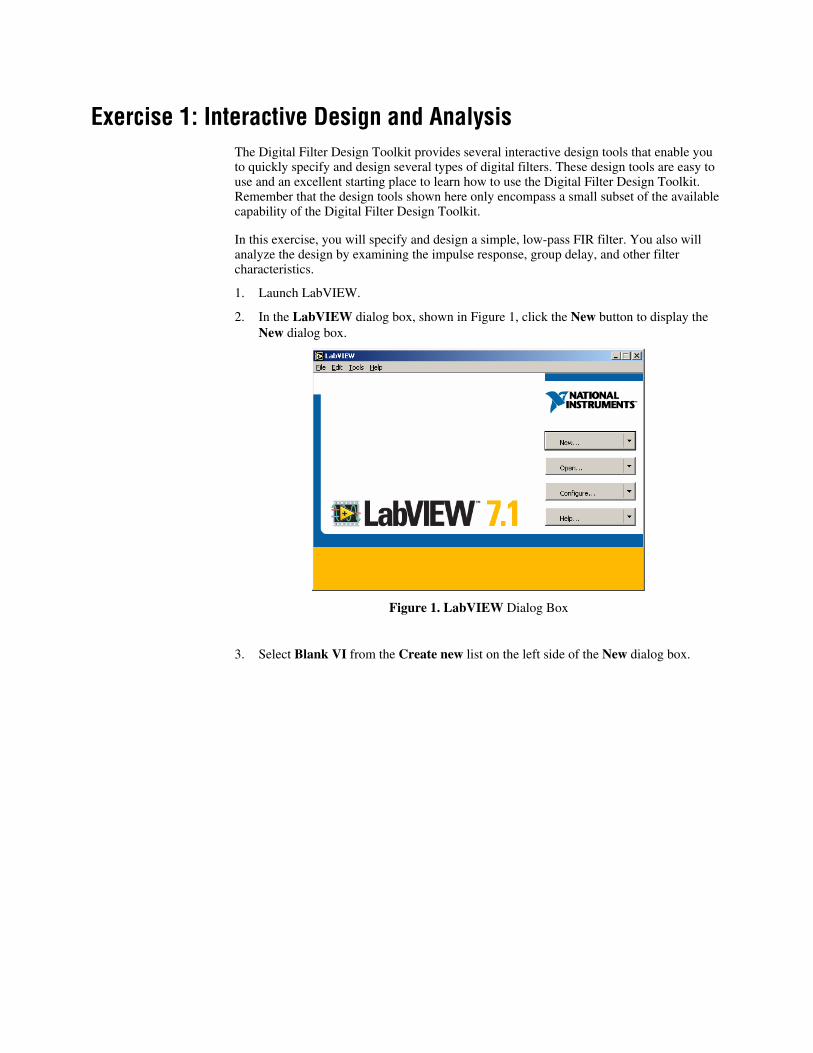
Exercise 1: Interactive Design and Analysis The Digital Filter Design Toolkit provides several interactive design tools that enable you to quickly specify and design several types of digital filters. These design tools are easy to use and an excellent starting place to learn how to use the Digital Filter Design Toolkit. Remember that the design tools shown here only encompass a small subset of the available capability of the Digital Filter Design Toolkit.

In this exercise, you will specify and design a simple, low-pass FIR filter. You also will analyze the design by examining the impulse response, group delay, and other filter characteristics.

1. Launch LabVIEW.

2. In the LabVIEW dialog box, shown in Figure 1, click the New button to display the New dialog box.

Figure 1. LabVIEW Dialog Box

3. Select Blank VI from the Create new list on the left side of the New dialog box.

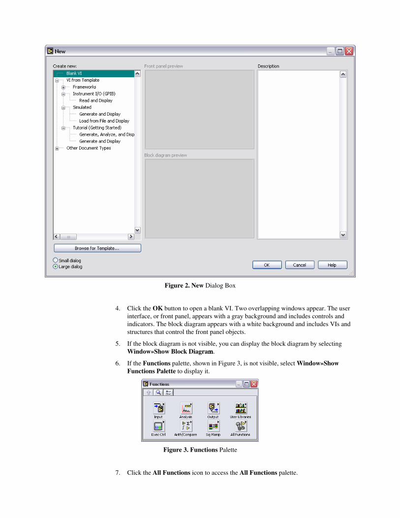
Figure 2. New Dialog Box

4. Click the OK button to open a blank VI. Two overlapping windows appear. The user interface, or front panel, appears with a gray background and includes controls and indicators. The block diagram appears with a white background and includes VIs and structures that control the front panel objects.

5. If the block diagram is not visible, you can display the block diagram by selecting Window»Show Block Diagrammmm.

6. If the Functions palette, shown in Figure 3, is not visible, select Window»Show Functions Palette to display it.

Figure 3. Functions Palette

7. Click the All Functions icon to access the All Functions palette.

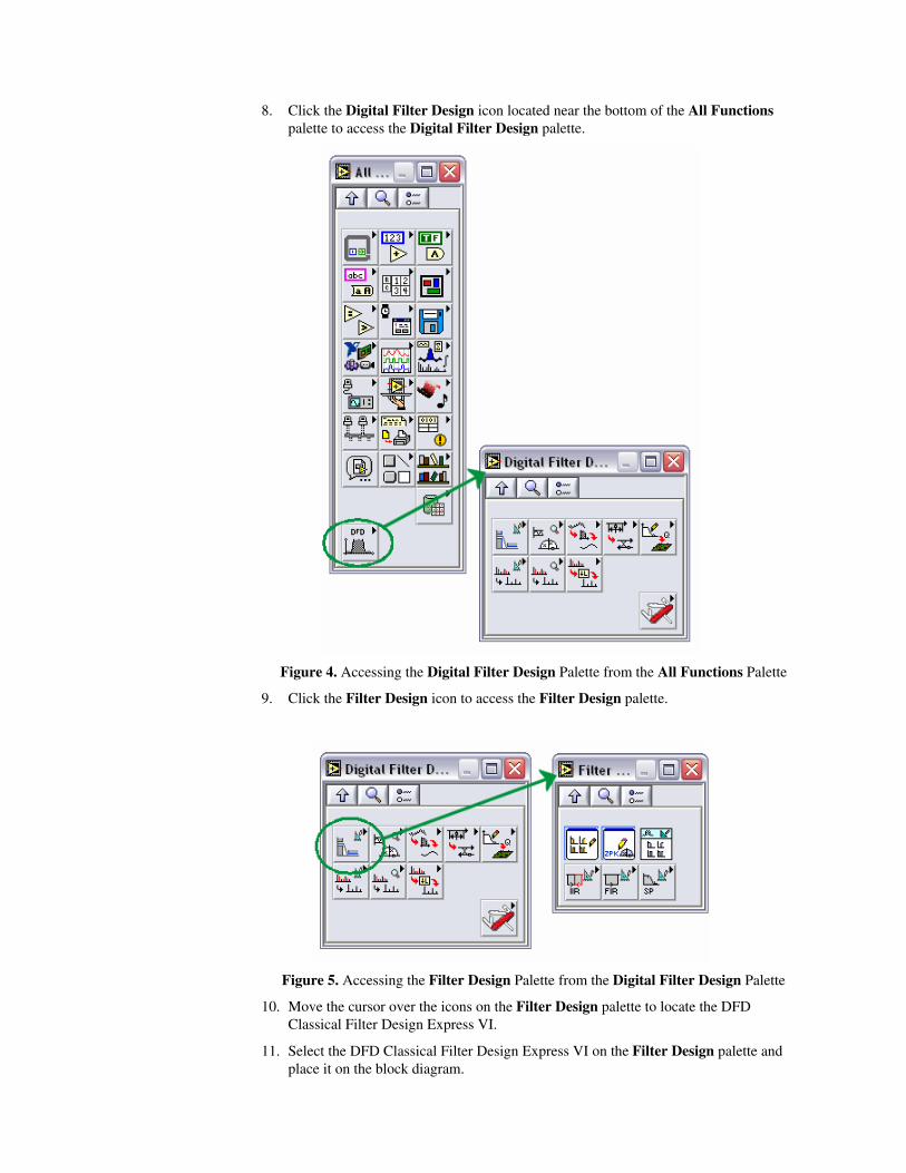
8. Click the Digital Filter Design icon located near the bottom of the All Functions palette to access the Digital Filter Design palette.

Figure 4. Accessing the Digital Filter Design Palette from the All Functions Palette

9. Click the Filter Design icon to access the Filter Design palette.

Figure 5. Accessing the Filter Design Palette from the Digital Filter Design Palette

10. Move the cursor over the icons on the Filter Design palette to locate the DFD Classical Filter Design Express VI.

11. Select the DFD Classical Filter Design Express VI on the Filter Design palette and place it on the block diagram.

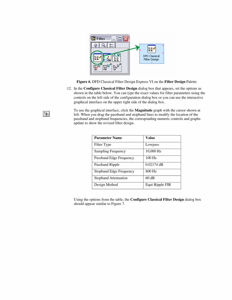
Figure 6. DFD Classical Filter Design Express VI on the Filter Design Palette

12. In the Configure Classical Filter Design dialog box that appears, set the options as shown in the table below. You can type the exact values for filter parameters using the controls on the left side of the configuration dialog box or you can use the interactive graphical interface on the upper right side of the dialog box.

To use the graphical interface, click the Magnitude graph with the cursor shown at left. When you drag the passband and stopband lines to modify the location of the passband and stopband frequencies, the corresponding numeric controls and graphs update to show the revised filter design.

Parameter Name Value

Filter Type Lowpass

Sampling Frequency 10,000 Hz

Passband Edge Frequency 100 Hz

Passband Ripple 0.02174 dB

Stopband Edge Frequency 800 Hz

Stopband Attenuation 60 dB

Design Method Equi-Ripple FIR

Using the options from the table, the Configure Classical Filter Design dialog box should appear similar to Figure 7.

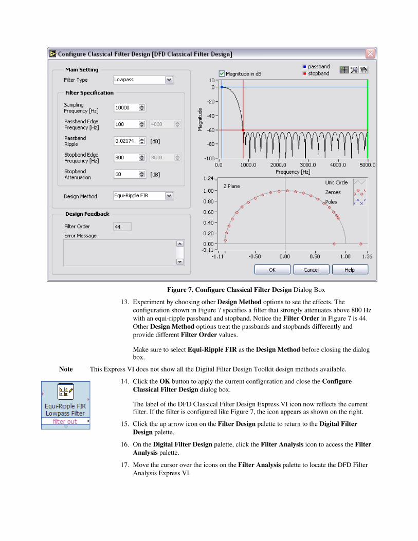
Figure 7. Configure Classical Filter Design Dialog Box

13. Experiment by choosing other Design Method options to see the effects. The configuration shown in Figure 7 specifies a filter that strongly attenuates above 800 Hz with an equi-ripple passband and stopband. Notice the Filter Order in Figure 7 is 44. Other Design Method options treat the passbands and stopbands differently and provide different Filter Order values.

Make sure to select Equi-Ripple FIR as the Design Method before closing the dialog box.

Note This Express VI does not show all the Digital Filter Design Toolkit design methods available.

14. Click the OK button to apply the current configuration and close the Configure Classical Filter Design dialog box.

The label of the DFD Classical Filter Design Express VI icon now reflects the current filter. If the filter is configured like Figure 7, the icon appears as shown on the right.

15. Click the up arrow icon on the Filter Design palette to return to the Digital Filter Design palette.

16. On the Digital Filter Design palette, click the Filter Analysis icon to access the Filter Analysis palette.

17. Move the cursor over the icons on the Filter Analysis palette to locate the DFD Filter Analysis Express VI.

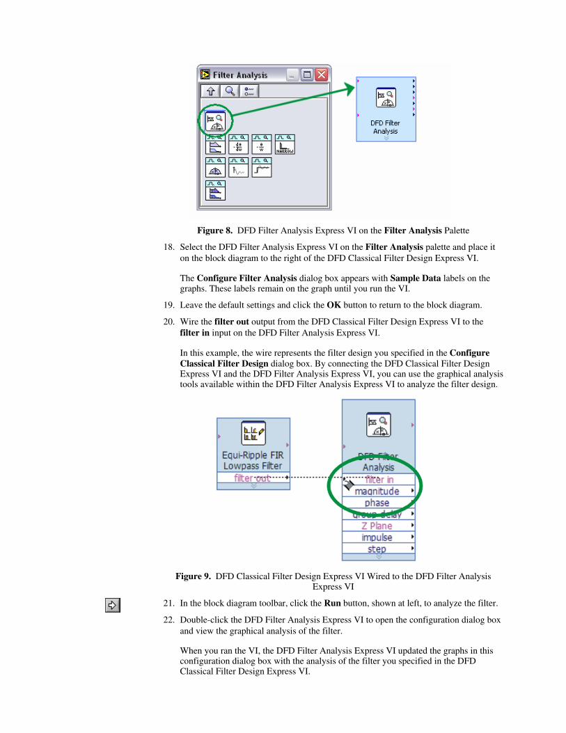
Figure 8. DFD Filter Analysis Express VI on the Filter Analysis Palette

18. Select the DFD Filter Analysis Express VI on the Filter Analysis palette and place it on the block diagram to the right of the DFD Classical Filter Design Express VI.

The Configure Filter Analysis dialog box appears with Sample Data labels on the graphs. These labels remain on the graph until you run the VI.

19. Leave the default settings and click the OK button to return to the block diagram.

20. Wire the filter out output from the DFD Classical Filter Design Express VI to the filter in input on the DFD Filter Analysis Express VI.

In this example, the wire represents the filter design you specified in the Configure Classical Filter Design dialog box. By connecting the DFD Classical Filter Design Express VI and the DFD Filter Analysis Express VI, you can use the graphical analysis tools available within the DFD Filter Analysis Express VI to analyze the filter design.

Figure 9. DFD Classical Filter Design Express VI Wired to the DFD Filter Analysis Express VI

21. In the block diagram toolbar, click the Run button, shown at left, to analyze the filter.

22. Double-click the DFD Filter Analysis Express VI to open the configuration dialog box and view the graphical analysis of the filter.

When you ran the VI, the DFD Filter Analysis Express VI updated the graphs in this configuration dialog box with the analysis of the filter you specified in the DFD Classical Filter Design Express VI.

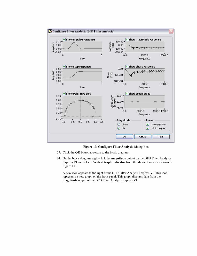
Figure 10. Configure Filter Analysis Dialog Box

23. Click the OK button to return to the block diagram.

24. On the block diagram, right-click the magnitude output on the DFD Filter Analysis Express VI and select Create»Graph Indicator from the shortcut menu as shown in Figure 11.

A new icon appears to the right of the DFD Filter Analysis Express VI. This icon represents a new graph on the front panel. This graph displays data from the magnitude output of the DFD Filter Analysis Express VI.

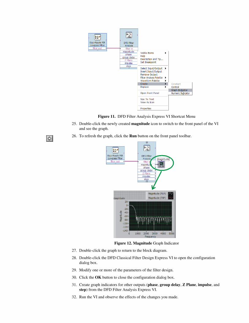
Figure 11. DFD Filter Analysis Express VI Shortcut Menu

25. Double-click the newly created magnitude icon to switch to the front panel of the VI and see the graph.

26. To refresh the graph, click the Run button on the front panel toolbar.

Figure 12. Magnitude Graph Indicator

27. Double-click the graph to return to the block diagram.

28. Double-click the DFD Classical Filter Design Express VI to open the configuration dialog box.

29. Modify one or more of the parameters of the filter design.

30. Click the OK button to close the configuration dialog box.

31. Create graph indicators for other outputs (phase, group delay, Z Plane, impulse, and step) from the DFD Filter Analysis Express VI.

32. Run the VI and observe the effects of the changes you made.

Exercise 2: Example VI Exploration The Digital Filter Design Toolkit installs more than 75 example VIs that cover a variety of digital filter design tools. In this exercise, you will explore some of these examples.

1. If you are continuing from the previous exercise, close any open VIs to return to the LabVIEW dialog box.

2. In the LabVIEW dialog box, click the triangle on the right side of the Open button and select Examples from the pull-down menu to launch the NI Example Finder. The NI Example Finder enables you to browse through LabVIEW example VIs.

By default, the NI Example Finder window lets you browse for example VIs according to task categories. The NI Example Finder displays these categories as folders in the middle of the NI Example Finder.

The NI Example Finder organizes the Digital Filter Design examples into categories that include:

• Case Study

• Conventional Filters

• Fixed-Point Filters

• Getting Started

• Multirate Filters

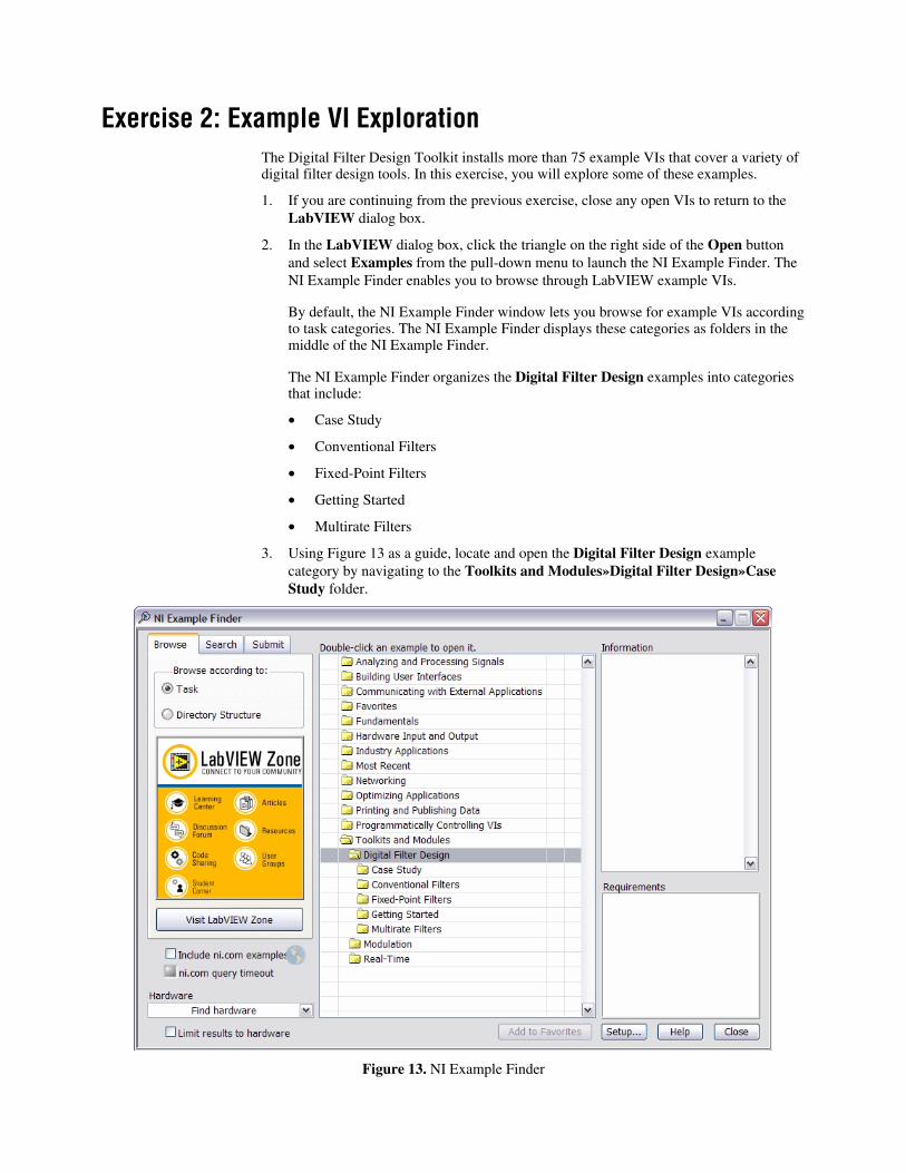
3. Using Figure 13 as a guide, locate and open the Digital Filter Design example category by navigating to the Toolkits and Modules»Digital Filter Design»Case Study folder.

Figure 13. NI Example Finder

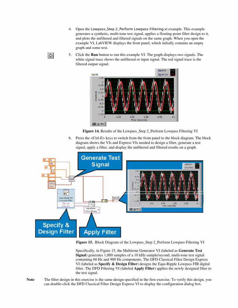
4. Open the Lowpass_Step 2_Perform Lowpass Filtering.vi example. This example generates a synthetic, multi-tone test signal, applies a floating-point filter design to it, and plots the unfiltered and filtered signals on the same graph. When you open the example VI, LabVIEW displays the front panel, which initially contains an empty graph and some text.

5. Click the Run button to run this example VI. The graph displays two signals. The white signal trace shows the unfiltered or input signal. The red signal trace is the filtered output signal.

Figure 14. Results of the Lowpass_Step 2_Perform Lowpass Filtering VI

6. Press the <Ctrl-E> keys to switch from the front panel to the block diagram. The block diagram shows the VIs and Express VIs needed to design a filter, generate a test signal, apply a filter, and display the unfiltered and filtered results on a graph.

Figure 15. Block Diagram of the Lowpass_Step 2_Perform Lowpass Filtering VI

Specifically, in Figure 15, the Multitone Generator VI (labeled as Generate Test Signal) generates 1,000 samples of a 10 kHz sample/second, multi-tone test signal containing 60 Hz and 900 Hz components. The DFD Classical Filter Design Express VI (labeled as Specify & Design Filter) designs the Equi-Ripple Lowpass FIR digital filter. The DFD Filtering VI (labeled Apply Filter) applies the newly designed filter to the test signal.

Note The filter design in this exercise is the same design specified in the first exercise. To verify this design, you can double-click the DFD Classical Filter Design Express VI to display the configuration dialog box.

7. Select Help»Find Examples from the pull-down menu in the toolbar to access the NI Example Finder.

8. Navigate to the Toolkits and Modules»Digital Filter Design»Getting Started folder.

9. Scroll through the list of example VIs and explore.

A References

This appendix lists references that contain more information about the theory and algorithms implemented in the LabVIEW Digital Filter Design Toolkit.

• Chugani, Mahesh L.; Abhay R. Samant; and Michael Cerna. LabVIEW Signal Processing. Upper Saddle River, NJ: Prentice Hall, 1998.

• Diniz, Paulo S. R.; Eduardo A. B. da Silva; and Sergio L Netto. Digital Signal Processing: System Analysis and Design. New York: Cambridge University Press, 2002.

• Hogenauer, E. B. “An economical class of digital filters for decimation and interpolation.” IEEE Transactions on Acoustics, Speech, and Signal Processing, ASSP-29 (2) (1981): 155–162.

• Ifeachor, E. C., and B. W. Jervis. Digital Signal Processing: A Practical Approach. 2d ed. Publishing House of Electronics Industry, 2003.

• Jayasimha, S., and P. V. R. N. Rao. “An iteration scheme for the design of equiripple Mth-band FIR filters.” IEEE Transactions on Signal Processing, vol. 43 (8) (Aug. 1995): 1998-2002.

• Mintzer, F. “On half-band, third-band, and nth-band FIR filters and their design.” IEEE Transactions on Acoustics, Speech, and Signal Processing, ASSP-30 (5) (October 1982): 734–738.

• Neuvo, Y; C-Y Dong; and S.K. Mitra. “Interpolated finite impulse response filters.” IEEE Transactions on Acoustics, Speech, and Signal Processing, ASSP-32 (June 1984): 563–570.

• Oppenheim, A. V., and R. W. Schafer. Discrete-Time Signal Processing. Englewood Cliffs, NJ: Prentice Hall, 1989.

• Orfanidis, S. J. Introduction to Signal Processing. Upper Saddle River, NJ: Prentice Hall, 1998.

• Parks, T. W., and C. S. Burrus. Digital Filter Design. New York: John Wiley & Sons, Inc., 1987.