Getting Started with STELLA v 6 - Sabancı Üniversitesipeople.sabanciuniv.edu/atilgan/StellaSoft/Guide/STELLA_Guide.pdf · Getting Started with STELLA ... The STELLA software is

Getting Started with STELLA® v 6.0

© MM High Performance Systems, Inc.The Systems Thinking Company TM

http://www.hps-inc.com

http://www.hps-inc.com/

© MM High Performance Systems, Inc. All rights reserved. 2

Table of Contents

Welcome

The Basics: A Tutorial for New Users 4

Appendix: Basic Software Operations & Features 36

RenderingIllustration 1: Depositing, Naming & Re-positioning Stocks, Converters 36 and Nameplates

Illustration 2: Hooking-up Flows 37

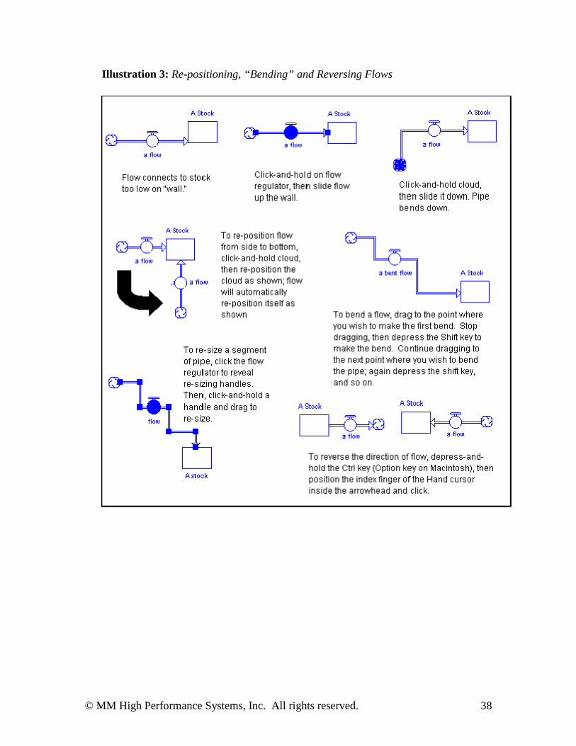
Illustration 3: Re-positioning, “Bending” and Reversing Flows 38

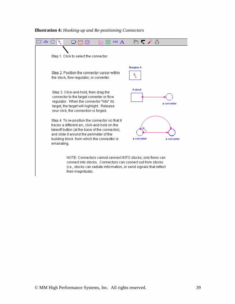
Illustration 4: Hooking-up and Re-positioning Connectors 39

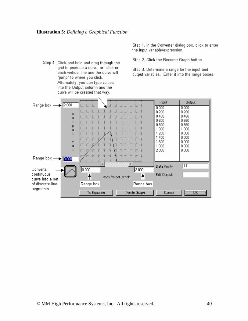
Illustration 5: Defining a Graphical Function 40

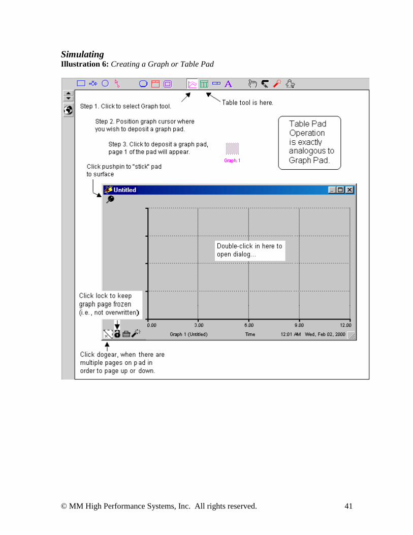
SimulatingIllustration 6: Creating a Graph or Table Pad 41

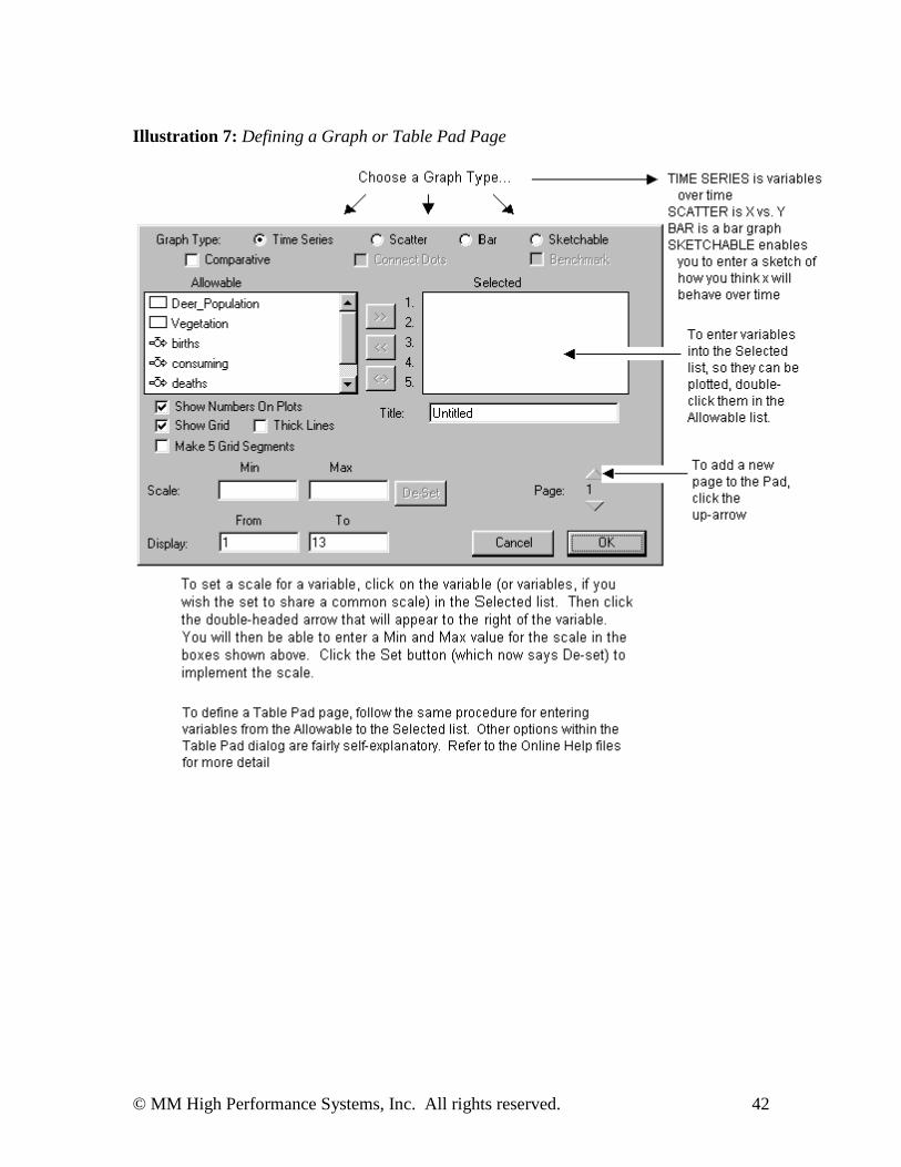
Illustration 7: Defining a Graph or Table Pad Page 42

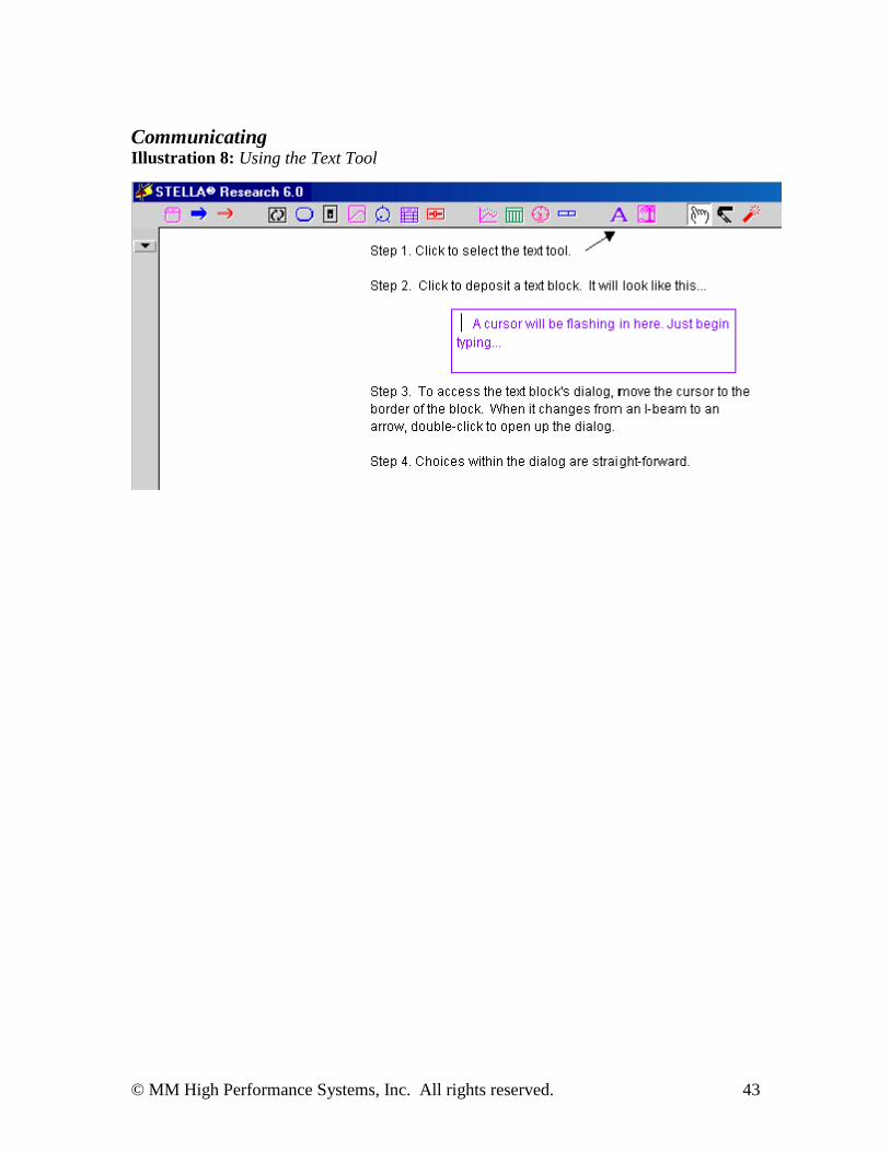
CommunicatingIllustration 8: Using the Text Tool 43


WelcomeWelcome to the STELLA® software “Getting Started” Tutorial! This tutorial provides anexperiential introduction to the basic operations and features of the STELLA software fornew users.

The STELLA Electronic Help Files that accompany the software comprehensivelydescribe software operation and features in much greater detail. The approach here isselective (not all features are illustrated), and context-rich. Through a case studyinvolving deer population, you’ll progress through an organized series of diagrams thatillustrate how to perform the basic operations and use the basic features of the software,associated with (1) rendering a mental model, (2) simulating the model to yielddynamic outputs, (3) analyzing the outputs to understand what’s causing them, and whatyou might do to change them, and (4) communicating your understanding by making theinsights derivable from the model available for “discovery” by others.

This tutorial is designed for users of both the STELLA Basic and Research versions ofthe software. The Research version was used to develop this tutorial. Those owning theBasic version might see some slightly different screen shots than the ones appearing inthe tutorial. Differences between the two versions will be identified as they arise.

The Basics will take you about an hour to complete. The tutorial is divided into sectionsso that if you choose to “take a break” and return later to complete the tutorial, noproblem. Have fun. Be cool (it would be hard not to, after mastering the basics of thissoftware!). Stay systemic.


The Basics: A Tutorial for New Users

The STELLA software is designed to increase the effectiveness of the set of processes bywhich we render, simulate, analyze and communicate our mental models. Mental modelsare those things we all necessarily carry around in our heads that help us to: (1) makemeaning out of what we experience, (2) share and evolve that meaning bycommunicating with others, and (3) evaluate and decide upon appropriate courses ofaction. As you can see, mental models are extremely important things. Learning toconstruct mental models that better reflect the reality they seek to mimic, and learning tosimulate them more reliably, are vital to making your world, and our world, work moreeffectively. The aim of the STELLA software is to accelerate and enrich these learningprocesses.

The context for mastering the basics of the software will be the rendering, simulating,analyzing and communicating of a mental model of deer population dynamics. Since weare seeking to build your basic expertise as quickly as possible, we will keep theillustrative example simple. By the time you complete the tutorial, you should see manyways that you might extend the example to capture more aspects of the deer populationdynamics. Please feel free to do so!

The approach we will take in this tutorial will be to show you a picture and then ask youto perform the software operations, or use the software features, needed to produce thepicture. The operations themselves are illustrated using a progression of screen-shotdiagrams that depict the processes of rendering, simulating, analyzing andcommunicating. The progression of diagrams appears in an Appendix that begins onp 35.

The Context

Population dynamics is a key content area in many social and physical science curricula.From one-celled organisms to human populations, a generic structure can be used as abasis for studying the dynamics of population growth and decline. In this tutorial, wewill examine the dynamics of a deer population in a (very) simple forest ecosystem.

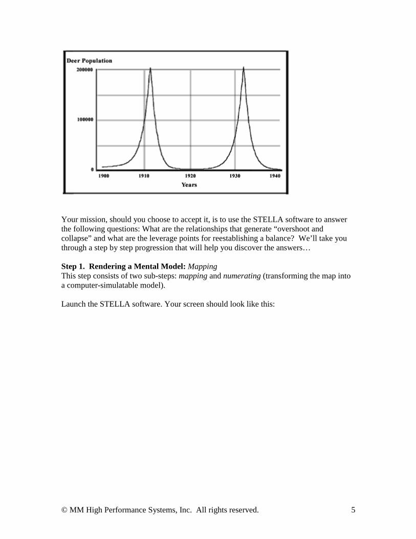
The deer population is regulated by food supply and predator population. In 1900, inresponse to pressures from ranchers and farmers, a $50 bounty was placed on predatorsbecause of attacks on livestock. In the next 40 years, an “overshoot and collapse” patternof growth and decline emerged in the deer population. The deer population grew until itfar exceeded what its food supply could support. Then, starvation on a massive scaleoccurred. This pattern can often occur in the natural world. The following graphillustrates the behavior of the population.


Your mission, should you choose to accept it, is to use the STELLA software to answerthe following questions: What are the relationships that generate “overshoot andcollapse” and what are the leverage points for reestablishing a balance? We’ll take youthrough a step by step progression that will help you discover the answers…

Step 1. Rendering a Mental Model: MappingThis step consists of two sub-steps: mapping and numerating (transforming the map intoa computer-simulatable model).

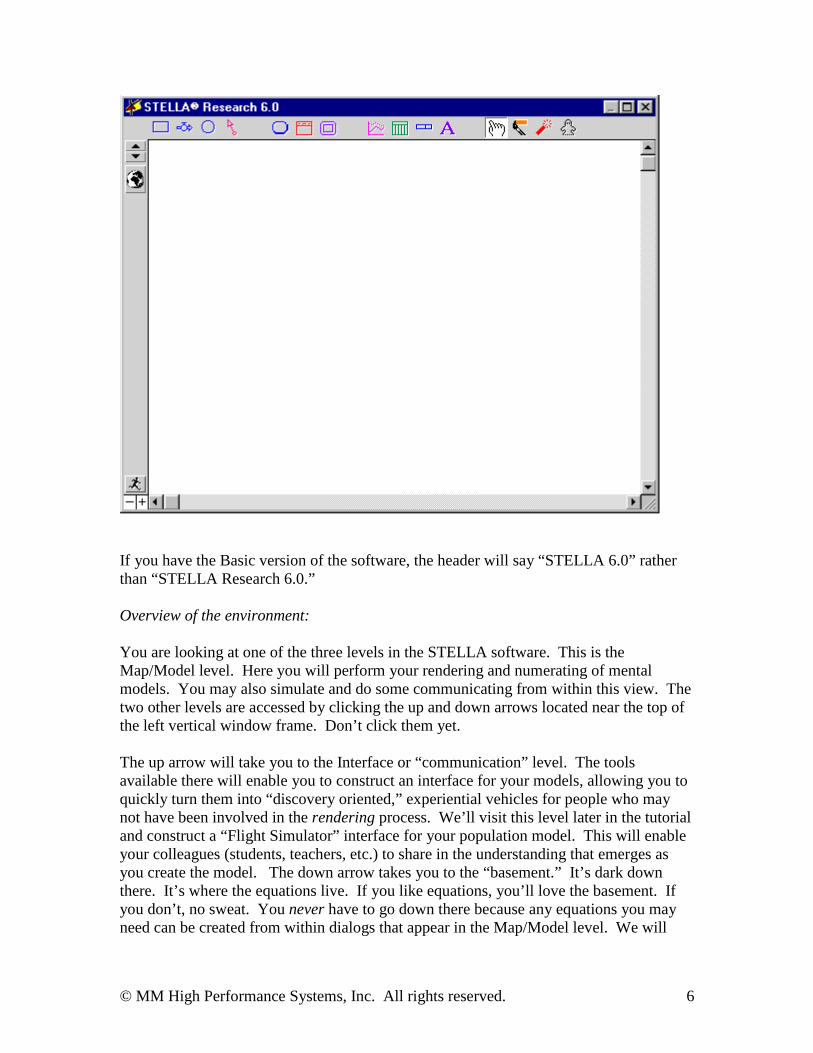
Launch the STELLA software. Your screen should look like this:


If you have the Basic version of the software, the header will say “STELLA 6.0” ratherthan “STELLA Research 6.0.”

Overview of the environment:

You are looking at one of the three levels in the STELLA software. This is theMap/Model level. Here you will perform your rendering and numerating of mentalmodels. You may also simulate and do some communicating from within this view. Thetwo other levels are accessed by clicking the up and down arrows located near the top ofthe left vertical window frame. Don’t click them yet.

The up arrow will take you to the Interface or “communication” level. The toolsavailable there will enable you to construct an interface for your models, allowing you toquickly turn them into “discovery oriented,” experiential vehicles for people who maynot have been involved in the rendering process. We’ll visit this level later in the tutorialand construct a “Flight Simulator” interface for your population model. This will enableyour colleagues (students, teachers, etc.) to share in the understanding that emerges asyou create the model. The down arrow takes you to the “basement.” It’s dark downthere. It’s where the equations live. If you like equations, you’ll love the basement. Ifyou don’t, no sweat. You never have to go down there because any equations you mayneed can be created from within dialogs that appear in the Map/Model level. We will


travel to the basement later in the tutorial. For now, hang with us on the Map/Modellevel.

Producing a first map:

It’s almost always a good idea to render a mental model, or a collective mental model (ifyou’re doing this in a group), in little chunks, one chunk at a time, rather than seeking tomap the whole thing at once. You spit out a little chunk, thinking about what you see asyou go. You then numerate, simulate, and ruminate on the results. Next, you spit outanother little chunk and repeat. Following this iterative, bite-sized approach will keepyou in control of the process. It’s very easy for the process to spin out of control becausethe software makes rendering so easy. In this part of the process, the software is acting asa “word processor for the mind.” Anyone can generate a lot of words with a wordprocessor. Writing a coherent essay, short story, or novel is quite another thingaltogether! The same is true with the STELLA software. Think quality, not quantity.Go slow, not fast. “Write” clear, simple mental models.

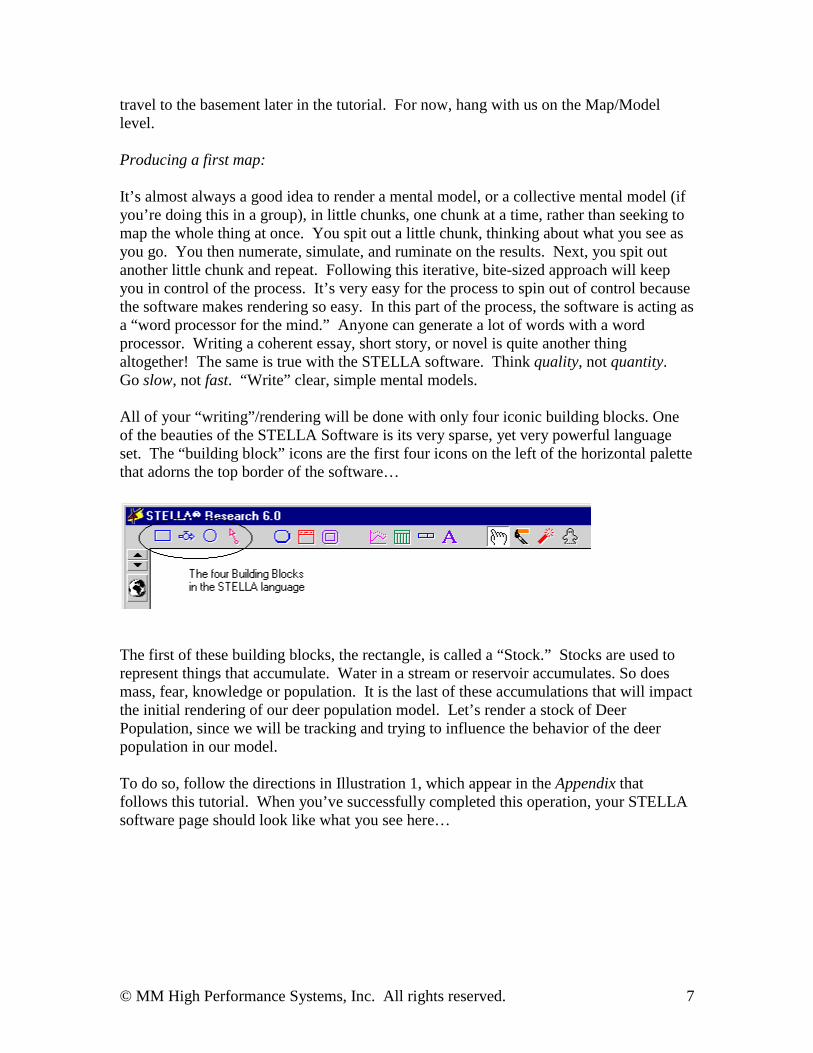
All of your “writing”/rendering will be done with only four iconic building blocks. Oneof the beauties of the STELLA Software is its very sparse, yet very powerful languageset. The “building block” icons are the first four icons on the left of the horizontal palettethat adorns the top border of the software…

The first of these building blocks, the rectangle, is called a “Stock.” Stocks are used torepresent things that accumulate. Water in a stream or reservoir accumulates. So doesmass, fear, knowledge or population. It is the last of these accumulations that will impactthe initial rendering of our deer population model. Let’s render a stock of DeerPopulation, since we will be tracking and trying to influence the behavior of the deerpopulation in our model.

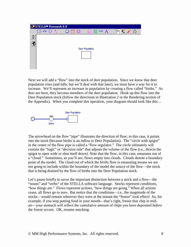
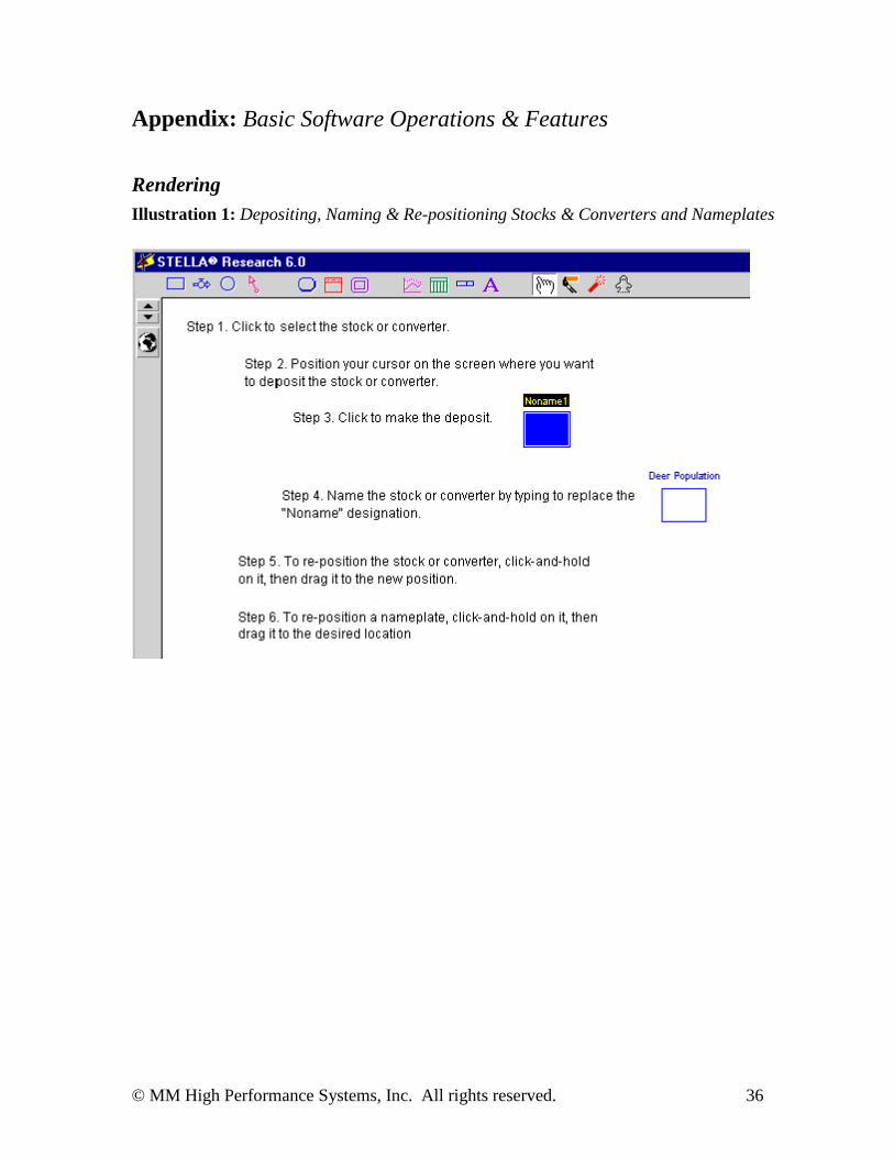
To do so, follow the directions in Illustration 1, which appear in the Appendix thatfollows this tutorial. When you’ve successfully completed this operation, your STELLAsoftware page should look like what you see here…


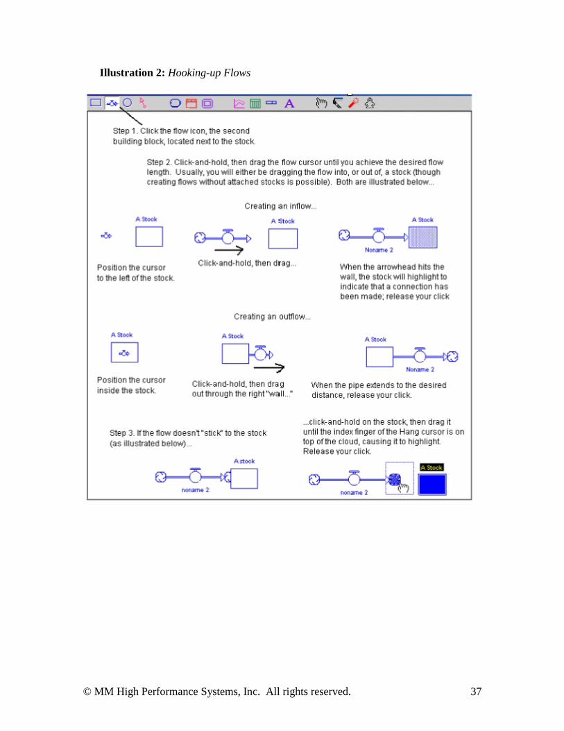
Next we will add a “flow” into the stock of deer population. Since we know that deerpopulation rises (and falls, but we’ll deal with that later), we must have a way for it toincrease. We’ll represent an increase in population by creating a flow called “births.” Asdeer are born, they become members of the deer population. Hook up this flow into theDeer Population stock (follow the directions in Illustration 2 in the Rendering section ofthe Appendix). When you complete this operation, your diagram should look like this…

The arrowhead on the flow “pipe” illustrates the direction of flow; in this case, it pointsinto the stock (because births is an inflow to Deer Population). The “circle with spigot”in the center of the flow pipe is called a “flow regulator.” The circle ultimately willcontain the “logic” or “decision rule” that adjusts the volume of the flow (i.e., directs thespigot to open wide or shut itself down). Note that the flow, in this case, emanates out ofa “cloud.” Sometimes, as you’ll see, flows empty into clouds. Clouds denote a boundarypoint of the model. The cloud out of which the births flow is emanating means we arenot going to include within the boundary of the model the source of the flow—the stockthat is being drained by the flow of births into the Deer Population stock.

Let’s pause briefly to savor the important distinction between a stock and a flow—the“nouns” and “verbs” of the STELLA software language. Stocks represent conditions,“how things are.” Flows represent actions, “how things are going.” When all actionscease, all flows go to zero. But notice that the conditions—i.e., the magnitude of thestocks—would remain wherever they were at the instant the “freeze” took effect! So, forexample, if you stop putting food in your mouth—that’s right, freeze that chip in mid-air—your stomach will reflect the cumulative amount of chips you have deposited beforethe freeze occurs. OK, resume snacking.


Recognizing the distinction between stocks and flows is absolutely critical to accuratelycapturing the dynamic behaviors a system will generate. We don’t have time to provide afull explanation here, but to get a quick glimpse of the differences, consider the basicstructure you just created. Can you see how it could be possible for the flow of births tobe increasing, but the Deer Population to actually be decreasing at the same time [Hint:consider the other side of the spectrum, the natural population control outflow known asdeath. We’ll be adding this flow to the map soon]? Without making the distinctionbetween stocks and flows, we would not be able to understand how the volume of a flowcould move in one direction while the magnitude of a stock moves in the oppositedirection.

By the way, you may notice that in our rendering of this map, we have used first-lettercaps when naming stocks, and all lower case for naming flows. This helps to make thedifference between these two types of variables more distinct, particularly when theyoccur in lists within dialogs, where we might not be able to see the different iconsassociated with each.

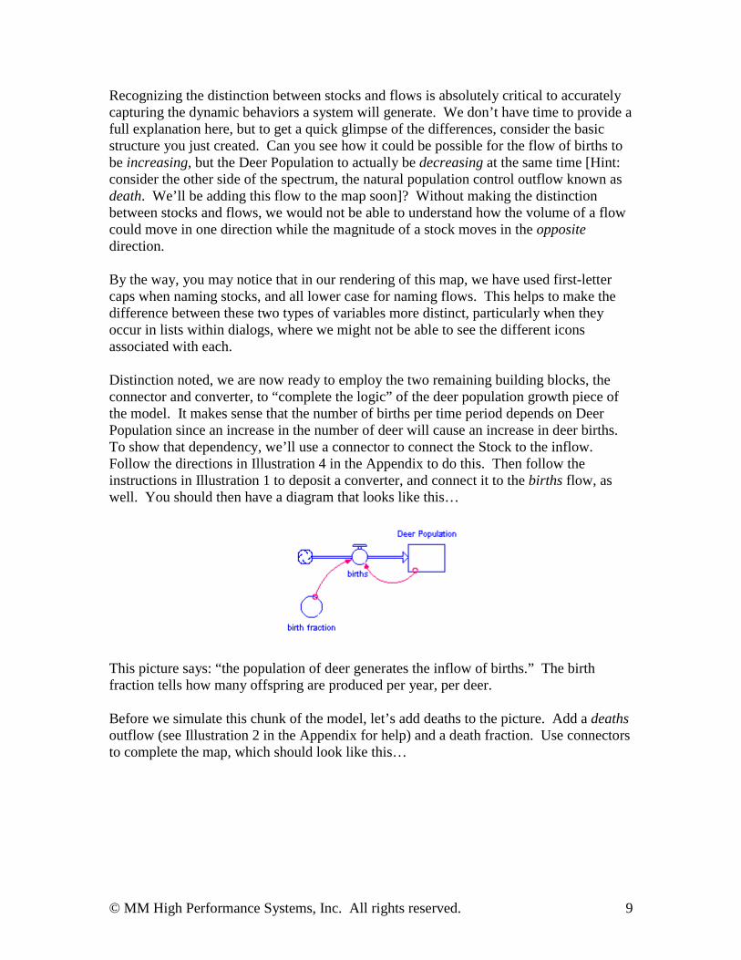
Distinction noted, we are now ready to employ the two remaining building blocks, theconnector and converter, to “complete the logic” of the deer population growth piece ofthe model. It makes sense that the number of births per time period depends on DeerPopulation since an increase in the number of deer will cause an increase in deer births.To show that dependency, we’ll use a connector to connect the Stock to the inflow.Follow the directions in Illustration 4 in the Appendix to do this. Then follow theinstructions in Illustration 1 to deposit a converter, and connect it to the births flow, aswell. You should then have a diagram that looks like this…

This picture says: “the population of deer generates the inflow of births.” The birthfraction tells how many offspring are produced per year, per deer.

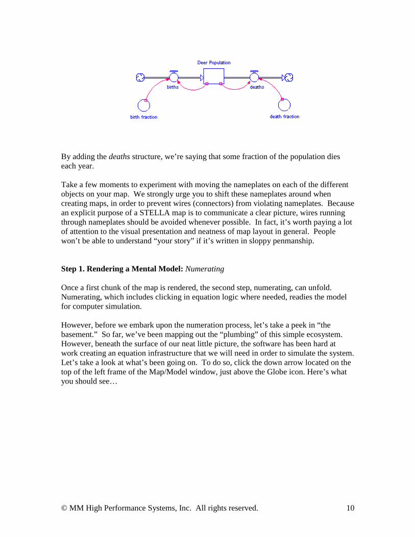
Before we simulate this chunk of the model, let’s add deaths to the picture. Add a deathsoutflow (see Illustration 2 in the Appendix for help) and a death fraction. Use connectorsto complete the map, which should look like this…


By adding the deaths structure, we’re saying that some fraction of the population dieseach year.

Take a few moments to experiment with moving the nameplates on each of the differentobjects on your map. We strongly urge you to shift these nameplates around whencreating maps, in order to prevent wires (connectors) from violating nameplates. Becausean explicit purpose of a STELLA map is to communicate a clear picture, wires runningthrough nameplates should be avoided whenever possible. In fact, it’s worth paying a lotof attention to the visual presentation and neatness of map layout in general. Peoplewon’t be able to understand “your story” if it’s written in sloppy penmanship.

Step 1. Rendering a Mental Model: Numerating

Once a first chunk of the map is rendered, the second step, numerating, can unfold.Numerating, which includes clicking in equation logic where needed, readies the modelfor computer simulation.

However, before we embark upon the numeration process, let’s take a peek in “thebasement.” So far, we’ve been mapping out the “plumbing” of this simple ecosystem.However, beneath the surface of our neat little picture, the software has been hard atwork creating an equation infrastructure that we will need in order to simulate the system.Let’s take a look at what’s been going on. To do so, click the down arrow located on thetop of the left frame of the Map/Model window, just above the Globe icon. Here’s whatyou should see…


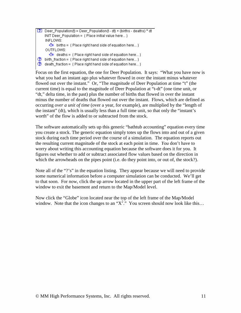
Focus on the first equation, the one for Deer Population. It says: “What you have now iswhat you had an instant ago plus whatever flowed in over the instant minus whateverflowed out over the instant.” Or, “The magnitude of Deer Population at time “t” (thecurrent time) is equal to the magnitude of Deer Population at “t-dt” (one time unit, or“dt,” delta time, in the past) plus the number of births that flowed in over the instantminus the number of deaths that flowed out over the instant. Flows, which are defined asoccurring over a unit of time (over a year, for example), are multiplied by the “length ofthe instant” (dt), which is usually less than a full time unit, so that only the “instant’sworth” of the flow is added to or subtracted from the stock.

The software automatically sets up this generic “bathtub accounting” equation every timeyou create a stock. The generic equation simply totes up the flows into and out of a givenstock during each time period over the course of a simulation. The equation reports outthe resulting current magnitude of the stock at each point in time. You don’t have toworry about writing this accounting equation because the software does it for you. Itfigures out whether to add or subtract associated flow values based on the direction inwhich the arrowheads on the pipes point (i.e. do they point into, or out of, the stock?).

Note all of the “?’s” in the equation listing. They appear because we will need to providesome numerical information before a computer simulation can be conducted. We’ll getto that soon. For now, click the up arrow located in the upper part of the left frame of thewindow to exit the basement and return to the Map/Model level.

Now click the “Globe” icon located near the top of the left frame of the Map/Modelwindow. Note that the icon changes to an “X2.” You screen should now look like this…


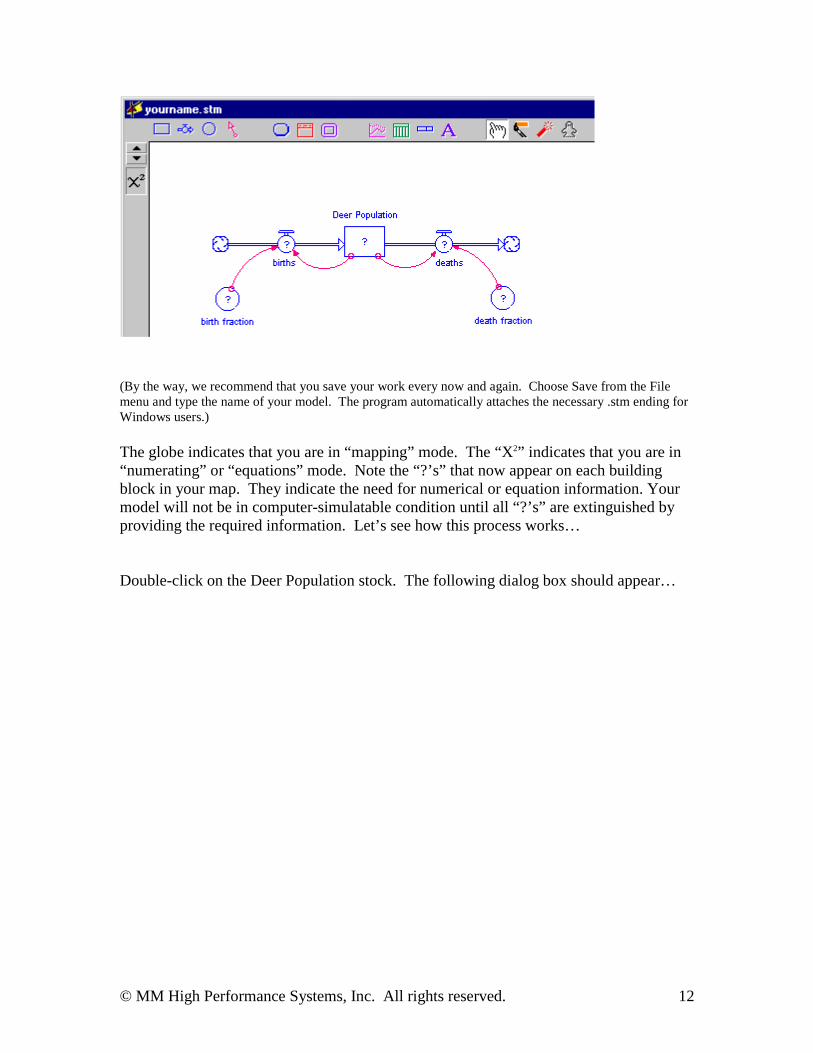
(By the way, we recommend that you save your work every now and again. Choose Save from the Filemenu and type the name of your model. The program automatically attaches the necessary .stm ending forWindows users.)

The globe indicates that you are in “mapping” mode. The “X2” indicates that you are in“numerating” or “equations” mode. Note the “?’s” that now appear on each buildingblock in your map. They indicate the need for numerical or equation information. Yourmodel will not be in computer-simulatable condition until all “?’s” are extinguished byproviding the required information. Let’s see how this process works…

Double-click on the Deer Population stock. The following dialog box should appear…


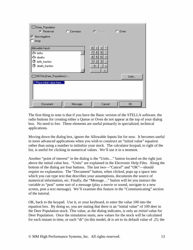
The first thing to note is that if you have the Basic version of the STELLA software, theradio buttons for creating either a Queue or Oven do not appear at the top of your dialogbox. No need to fret. These elements are useful primarily in specialized, technicalapplications.

Moving down the dialog box, ignore the Allowable Inputs list for now. It becomes usefulin more advanced applications when you wish to construct an “initial value” equationrather than using a number to initialize your stock. The calculator keypad, to right of thelist, is useful for clicking in numerical values. We’ll use it in a moment.

Another “point of interest” in the dialog is the “Units…” button located on the right justabove the initial value box. “Units” are explained in the Electronic Help Files. Along thebottom of the dialog are four buttons. The last two—“Cancel” and “OK”—shouldrequire no explanation. The “Document” button, when clicked, pops up a space intowhich you can type text that describes your assumptions, documents the source ofnumerical information, etc. Finally, the “Message…” button will let you instruct thevariable to “post” some sort of a message (play a movie or sound, navigate to a newscreen, post a text message). We’ll examine this feature in the “Communicating” sectionof the tutorial.

OK, back to the keypad. Use it, or your keyboard, to enter the value 100 into theequation box. By doing so, you are stating that there is an “initial value” of 100 deer inthe Deer Population stock. This value, as the dialog indicates, is only an initial value forDeer Population. Once the simulation starts, new values for the stock will be calculatedfor each instant in time, or each “dt” (in this model, dt is set to its default value of .25; the


simulation will make calculations each ¼ of a time period—which is, in this model, amonth). Once the 100 is entered, click OK to exit the dialog.

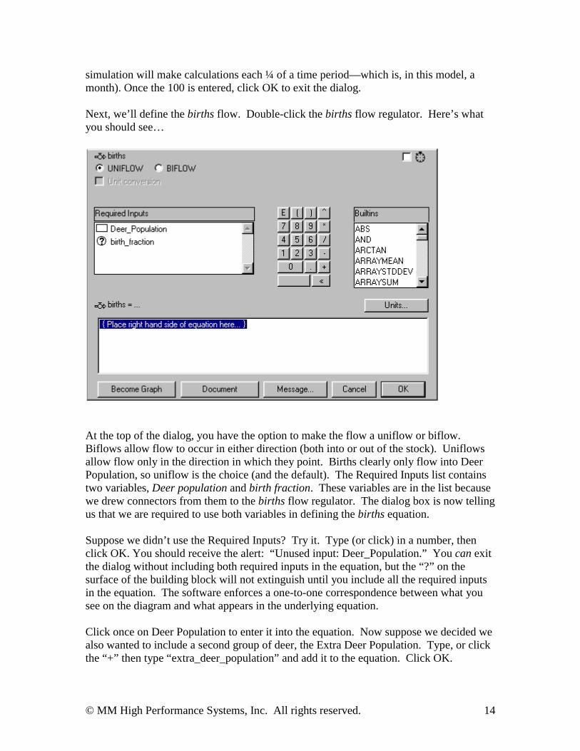
Next, we’ll define the births flow. Double-click the births flow regulator. Here’s whatyou should see…

At the top of the dialog, you have the option to make the flow a uniflow or biflow.Biflows allow flow to occur in either direction (both into or out of the stock). Uniflowsallow flow only in the direction in which they point. Births clearly only flow into DeerPopulation, so uniflow is the choice (and the default). The Required Inputs list containstwo variables, Deer population and birth fraction. These variables are in the list becausewe drew connectors from them to the births flow regulator. The dialog box is now tellingus that we are required to use both variables in defining the births equation.

Suppose we didn’t use the Required Inputs? Try it. Type (or click) in a number, thenclick OK. You should receive the alert: “Unused input: Deer_Population.” You can exitthe dialog without including both required inputs in the equation, but the “?” on thesurface of the building block will not extinguish until you include all the required inputsin the equation. The software enforces a one-to-one correspondence between what yousee on the diagram and what appears in the underlying equation.

Click once on Deer Population to enter it into the equation. Now suppose we decided wealso wanted to include a second group of deer, the Extra Deer Population. Type, or clickthe “+” then type “extra_deer_population” and add it to the equation. Click OK.


You should receive the message: “Not the name of any object on the Diagram.” Thesoftware not only ensures that what you see is what you get, it also ensures that if youdon’t see it, you don’t get it! If you wish to include a variable in an equation, you need toinclude that variable in the map. Delete “+extra_deer_population” from the equation andtype (or click) the “*” and click once on birth fraction. The equation box should nowread as follows:

Deer_Population*birth_fraction

Click OK to exit the dialog. Note that there are no longer “?’s” on either the stock ofDeer Population or the births flow.

Let’s assume that for every 10 deer in the ecosystem, two deer will be born every year.Therefore, the birth fraction in this system is 2/10 or .20. Double-click on the birthfraction converter and type or click in the value of .20. Click OK to exit the dialog.

Fill in the remaining equations and inputs as follows:

deaths: Deer_Population*death_fractiondeath fraction: .02

Your model should now be ready to simulate—there should be no “?” remaining in themap.

Step 2. Simulating

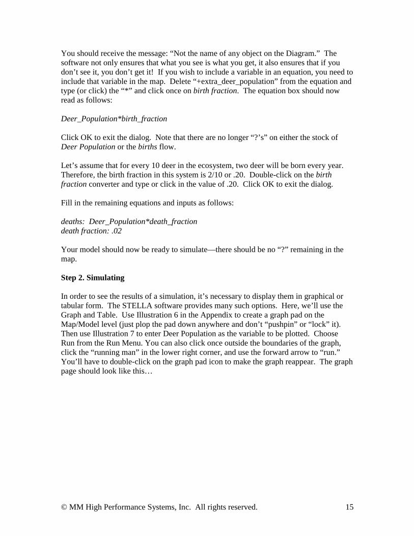
In order to see the results of a simulation, it’s necessary to display them in graphical ortabular form. The STELLA software provides many such options. Here, we’ll use theGraph and Table. Use Illustration 6 in the Appendix to create a graph pad on theMap/Model level (just plop the pad down anywhere and don’t “pushpin” or “lock” it).Then use Illustration 7 to enter Deer Population as the variable to be plotted. ChooseRun from the Run Menu. You can also click once outside the boundaries of the graph,click the “running man” in the lower right corner, and use the forward arrow to “run.”You’ll have to double-click on the graph pad icon to make the graph reappear. The graphpage should look like this…


Actually, your graph won’t look exactly like this. The numerical scale for DeerPopulation has been reformatted to remove the two decimal points from the scale. If youwish to reformat the variable, make sure you have exited the graph dialog, then double-click on “Deer Population” on top of the graph page to pop-up the formatting dialog box,and choose “0.” Also, make sure that you have scaled the Y-axis to begin at 0 and end at1500. See Illustration 7 in the Appendix for help.

You may also use the Paintbrush (located on the tool palette next to the Hand), to coloreither the graph pad page or the variables being displayed. Just click and hold on thePaintbrush, then select a color from the palette that appears. Next, click the page orvariable to color it.

Another nice feature of the Graph Pad page is that by clicking and holding on a point onany curve/line on the page, the associated numerical value of the variable at that point intime will be displayed underneath the variable name. Try it, you’ll like it!

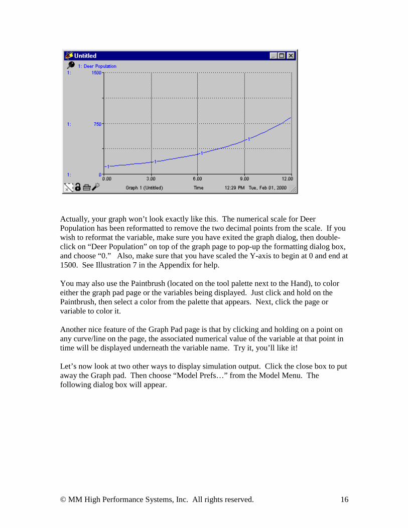
Let’s now look at two other ways to display simulation output. Click the close box to putaway the Graph pad. Then choose “Model Prefs…” from the Model Menu. Thefollowing dialog box will appear.


Note that in the dialog shown here the three building block icons under the word“Animate” have boxes around them. By clicking each icon, you too can make theseboxes appear. Do so now, then OK the dialog box.

Click the forward button on your run controller and observe. OK, so this is not a veryexciting animation…at least not yet. The only action is the stock of deer filling up.Don’t worry, things will get more interesting.

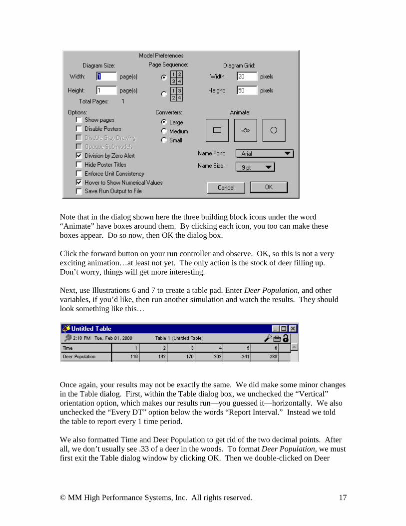
Next, use Illustrations 6 and 7 to create a table pad. Enter Deer Population, and othervariables, if you’d like, then run another simulation and watch the results. They shouldlook something like this…

Once again, your results may not be exactly the same. We did make some minor changesin the Table dialog. First, within the Table dialog box, we unchecked the “Vertical”orientation option, which makes our results run—you guessed it—horizontally. We alsounchecked the “Every DT” option below the words “Report Interval.” Instead we toldthe table to report every 1 time period.

We also formatted Time and Deer Population to get rid of the two decimal points. Afterall, we don’t usually see .33 of a deer in the woods. To format Deer Population, we mustfirst exit the Table dialog window by clicking OK. Then we double-clicked on Deer


Population in the Table and chose a precision of 0. We did the same for Time. Runagain and your results should be identical to those shown on the previous page.

Step 3. Analyzing

So, now that we’ve simulated, what can we learn from our model? What we’ve observedso far does not conform to the “overshoot and collapse” phenomenon that we saw at thebeginning of the exercise. Instead, we see smooth, exponential growth. Why don’t wesee “overshoot and collapse?” Is it possible for this very simple structure to generategrowth and subsequent decline in population? Fortunately, the software providespowerful tools for answering these sorts of questions. In this case, let’s use SensitivityAnalysis to see if our model can generate “overshoot and collapse.”

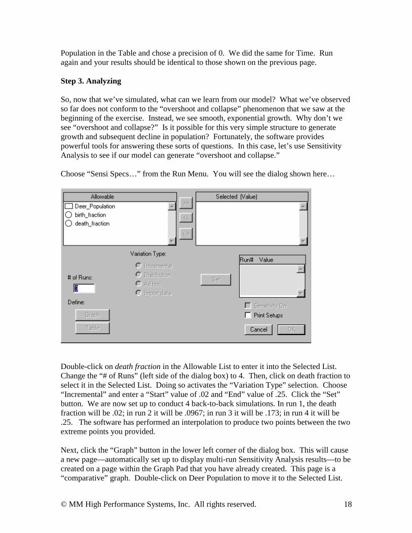
Choose “Sensi Specs…” from the Run Menu. You will see the dialog shown here…

Double-click on death fraction in the Allowable List to enter it into the Selected List.Change the “# of Runs” (left side of the dialog box) to 4. Then, click on death fraction toselect it in the Selected List. Doing so activates the “Variation Type” selection. Choose“Incremental” and enter a “Start” value of .02 and “End” value of .25. Click the “Set”button. We are now set up to conduct 4 back-to-back simulations. In run 1, the deathfraction will be .02; in run 2 it will be .0967; in run 3 it will be .173; in run 4 it will be.25. The software has performed an interpolation to produce two points between the twoextreme points you provided.

Next, click the “Graph” button in the lower left corner of the dialog box. This will causea new page—automatically set up to display multi-run Sensitivity Analysis results—to becreated on a page within the Graph Pad that you have already created. This page is a“comparative” graph. Double-click on Deer Population to move it to the Selected List.


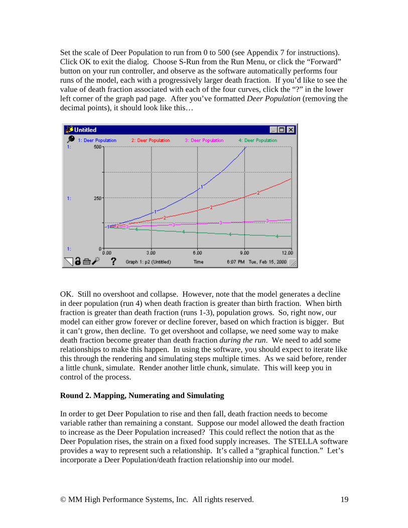
Set the scale of Deer Population to run from 0 to 500 (see Appendix 7 for instructions).Click OK to exit the dialog. Choose S-Run from the Run Menu, or click the “Forward”button on your run controller, and observe as the software automatically performs fourruns of the model, each with a progressively larger death fraction. If you’d like to see thevalue of death fraction associated with each of the four curves, click the “?” in the lowerleft corner of the graph pad page. After you’ve formatted Deer Population (removing thedecimal points), it should look like this…

OK. Still no overshoot and collapse. However, note that the model generates a declinein deer population (run 4) when death fraction is greater than birth fraction. When birthfraction is greater than death fraction (runs 1-3), population grows. So, right now, ourmodel can either grow forever or decline forever, based on which fraction is bigger. Butit can’t grow, then decline. To get overshoot and collapse, we need some way to makedeath fraction become greater than death fraction during the run. We need to add somerelationships to make this happen. In using the software, you should expect to iterate likethis through the rendering and simulating steps multiple times. As we said before, rendera little chunk, simulate. Render another little chunk, simulate. This will keep you incontrol of the process.

Round 2. Mapping, Numerating and Simulating

In order to get Deer Population to rise and then fall, death fraction needs to becomevariable rather than remaining a constant. Suppose our model allowed the death fractionto increase as the Deer Population increased? This could reflect the notion that as theDeer Population rises, the strain on a fixed food supply increases. The STELLA softwareprovides a way to represent such a relationship. It’s called a “graphical function.” Let’sincorporate a Deer Population/death fraction relationship into our model.


Draw a connector from Deer Population to death fraction, as shown below.

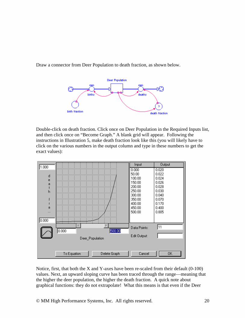
Double-click on death fraction. Click once on Deer Population in the Required Inputs list,and then click once on “Become Graph.” A blank grid will appear. Following theinstructions in Illustration 5, make death fraction look like this (you will likely have toclick on the various numbers in the output column and type in these numbers to get theexact values):

Notice, first, that both the X and Y-axes have been re-scaled from their default (0-100)values. Next, an upward sloping curve has been traced through the range—meaning thatthe higher the deer population, the higher the death fraction. A quick note aboutgraphical functions: they do not extrapolate! What this means is that even if the Deer


Population goes above 500, the death fraction in our illustrative graphical function willremain at .805, the maximum value defined by the graphical function.

Click OK to exit the graphical function dialog. Your map should now be free of “?’s,”and a tiny squiggle should appear in the death fraction converter, indicating that thisvalue is now a graphical function.

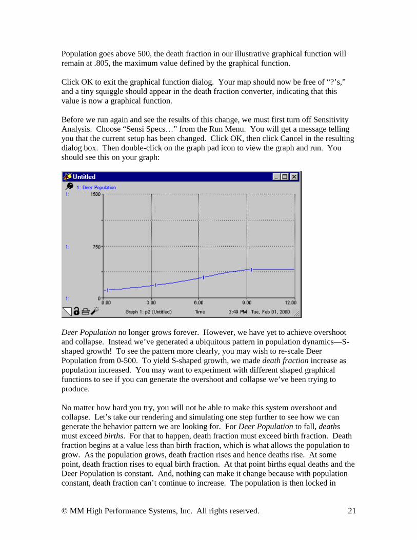
Before we run again and see the results of this change, we must first turn off SensitivityAnalysis. Choose “Sensi Specs…” from the Run Menu. You will get a message tellingyou that the current setup has been changed. Click OK, then click Cancel in the resultingdialog box. Then double-click on the graph pad icon to view the graph and run. Youshould see this on your graph:

Deer Population no longer grows forever. However, we have yet to achieve overshootand collapse. Instead we’ve generated a ubiquitous pattern in population dynamics—S-shaped growth! To see the pattern more clearly, you may wish to re-scale DeerPopulation from 0-500. To yield S-shaped growth, we made death fraction increase aspopulation increased. You may want to experiment with different shaped graphicalfunctions to see if you can generate the overshoot and collapse we’ve been trying toproduce.

No matter how hard you try, you will not be able to make this system overshoot andcollapse. Let’s take our rendering and simulating one step further to see how we cangenerate the behavior pattern we are looking for. For Deer Population to fall, deathsmust exceed births. For that to happen, death fraction must exceed birth fraction. Deathfraction begins at a value less than birth fraction, which is what allows the population togrow. As the population grows, death fraction rises and hence deaths rise. At somepoint, death fraction rises to equal birth fraction. At that point births equal deaths and theDeer Population is constant. And, nothing can make it change because with populationconstant, death fraction can’t continue to increase. The population is then locked in


steady-state. In order for death fraction to rise above birth fraction, it must depend onsomething other than Deer Population. For example, consider making it depend on afood source (vegetation). As population rises, it consumes vegetation more and morerapidly. Eventually, as vegetation runs out, deaths will skyrocket. Let’s add vegetationto the model.

Round 3. Mapping, Numerating and Simulating

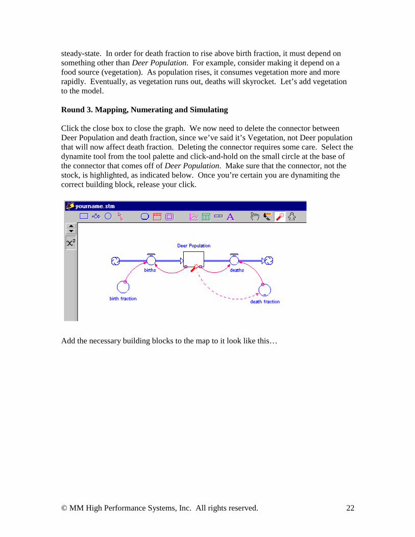
Click the close box to close the graph. We now need to delete the connector betweenDeer Population and death fraction, since we’ve said it’s Vegetation, not Deer populationthat will now affect death fraction. Deleting the connector requires some care. Select thedynamite tool from the tool palette and click-and-hold on the small circle at the base ofthe connector that comes off of Deer Population. Make sure that the connector, not thestock, is highlighted, as indicated below. Once you’re certain you are dynamiting thecorrect building block, release your click.

Add the necessary building blocks to the map to it look like this…


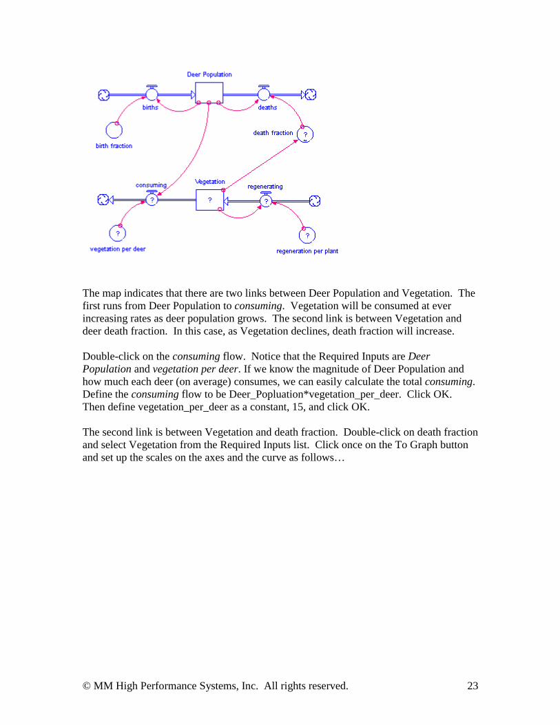
The map indicates that there are two links between Deer Population and Vegetation. Thefirst runs from Deer Population to consuming. Vegetation will be consumed at everincreasing rates as deer population grows. The second link is between Vegetation anddeer death fraction. In this case, as Vegetation declines, death fraction will increase.

Double-click on the consuming flow. Notice that the Required Inputs are DeerPopulation and vegetation per deer. If we know the magnitude of Deer Population andhow much each deer (on average) consumes, we can easily calculate the total consuming.Define the consuming flow to be Deer_Popluation*vegetation_per_deer. Click OK.Then define vegetation_per_deer as a constant, 15, and click OK.

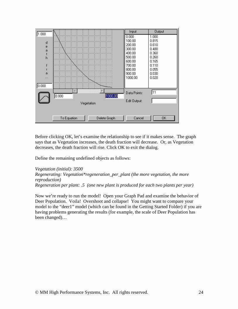
The second link is between Vegetation and death fraction. Double-click on death fractionand select Vegetation from the Required Inputs list. Click once on the To Graph buttonand set up the scales on the axes and the curve as follows…


Before clicking OK, let’s examine the relationship to see if it makes sense. The graphsays that as Vegetation increases, the death fraction will decrease. Or, as Vegetationdecreases, the death fraction will rise. Click OK to exit the dialog.

Define the remaining undefined objects as follows:

Vegetation (initial): 3500Regenerating: Vegetation*regeneration_per_plant (the more vegetation, the morereproduction)Regeneration per plant: .5 (one new plant is produced for each two plants per year)

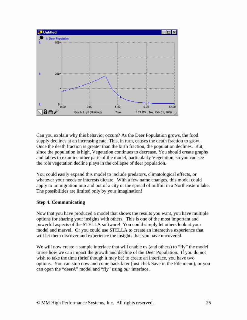
Now we’re ready to run the model! Open your Graph Pad and examine the behavior ofDeer Population. Voila! Overshoot and collapse! You might want to compare yourmodel to the “deer1” model (which can be found in the Getting Started Folder) if you arehaving problems generating the results (for example, the scale of Deer Population hasbeen changed)…


Can you explain why this behavior occurs? As the Deer Population grows, the foodsupply declines at an increasing rate. This, in turn, causes the death fraction to grow.Once the death fraction is greater than the birth fraction, the population declines. But,since the population is high, Vegetation continues to decrease. You should create graphsand tables to examine other parts of the model, particularly Vegetation, so you can seethe role vegetation decline plays in the collapse of deer population.

You could easily expand this model to include predators, climatological effects, orwhatever your needs or interests dictate. With a few name changes, this model couldapply to immigration into and out of a city or the spread of milfoil in a Northeastern lake.The possibilities are limited only by your imagination!

Step 4. Communicating

Now that you have produced a model that shows the results you want, you have multipleoptions for sharing your insights with others. This is one of the most important andpowerful aspects of the STELLA software! You could simply let others look at yourmodel and marvel. Or you could use STELLA to create an interactive experience thatwill let them discover and experience the insights that you have uncovered.

We will now create a sample interface that will enable us (and others) to “fly” the modelto see how we can impact the growth and decline of the Deer Population. If you do notwish to take the time (brief though it may be) to create an interface, you have twooptions. You can stop now and come back later (just click Save in the File menu), or youcan open the “deerA” model and “fly” using our interface.


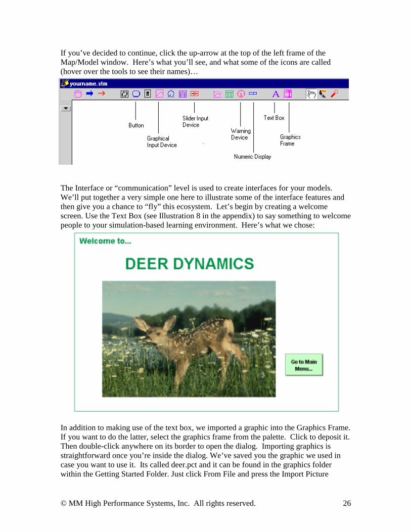
If you’ve decided to continue, click the up-arrow at the top of the left frame of theMap/Model window. Here’s what you’ll see, and what some of the icons are called(hover over the tools to see their names)…

The Interface or “communication” level is used to create interfaces for your models.We’ll put together a very simple one here to illustrate some of the interface features andthen give you a chance to “fly” this ecosystem. Let’s begin by creating a welcomescreen. Use the Text Box (see Illustration 8 in the appendix) to say something to welcomepeople to your simulation-based learning environment. Here’s what we chose:

In addition to making use of the text box, we imported a graphic into the Graphics Frame.If you want to do the latter, select the graphics frame from the palette. Click to deposit it.Then double-click anywhere on its border to open the dialog. Importing graphics isstraightforward once you’re inside the dialog. We’ve saved you the graphic we used incase you want to use it. Its called deer.pct and it can be found in the graphics folderwithin the Getting Started Folder. Just click From File and press the Import Picture


button. Navigate to the deer.pct file (found in your Graphics folder contained within theGetting Started with STELLA folder) and click Open. Then click OK to exit the dialogbox.

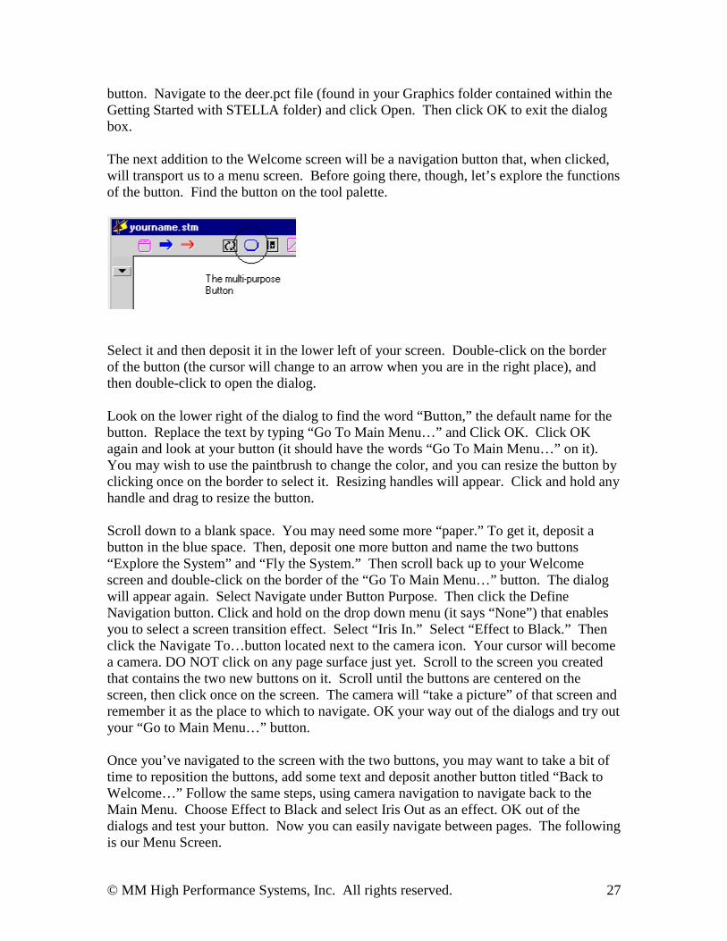
The next addition to the Welcome screen will be a navigation button that, when clicked,will transport us to a menu screen. Before going there, though, let’s explore the functionsof the button. Find the button on the tool palette.

Select it and then deposit it in the lower left of your screen. Double-click on the borderof the button (the cursor will change to an arrow when you are in the right place), andthen double-click to open the dialog.

Look on the lower right of the dialog to find the word “Button,” the default name for thebutton. Replace the text by typing “Go To Main Menu…” and Click OK. Click OKagain and look at your button (it should have the words “Go To Main Menu…” on it).You may wish to use the paintbrush to change the color, and you can resize the button byclicking once on the border to select it. Resizing handles will appear. Click and hold anyhandle and drag to resize the button.

Scroll down to a blank space. You may need some more “paper.” To get it, deposit abutton in the blue space. Then, deposit one more button and name the two buttons“Explore the System” and “Fly the System.” Then scroll back up to your Welcomescreen and double-click on the border of the “Go To Main Menu…” button. The dialogwill appear again. Select Navigate under Button Purpose. Then click the DefineNavigation button. Click and hold on the drop down menu (it says “None”) that enablesyou to select a screen transition effect. Select “Iris In.” Select “Effect to Black.” Thenclick the Navigate To…button located next to the camera icon. Your cursor will becomea camera. DO NOT click on any page surface just yet. Scroll to the screen you createdthat contains the two new buttons on it. Scroll until the buttons are centered on thescreen, then click once on the screen. The camera will “take a picture” of that screen andremember it as the place to which to navigate. OK your way out of the dialogs and try outyour “Go to Main Menu…” button.

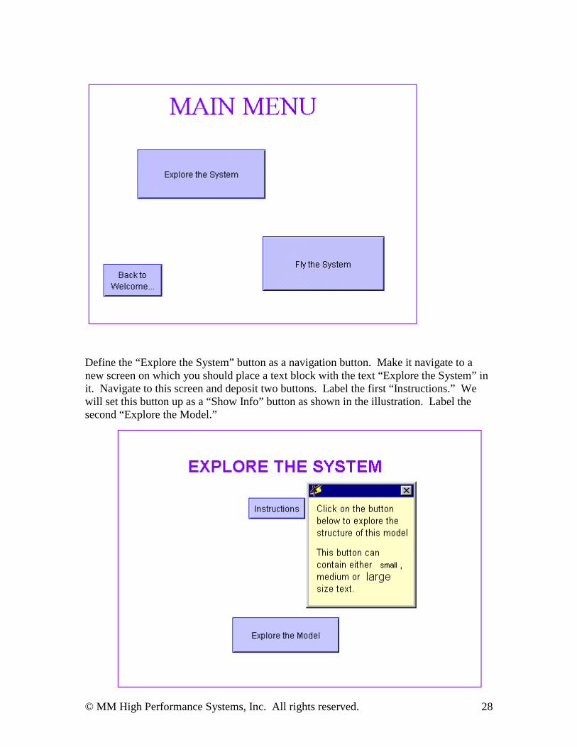
Once you’ve navigated to the screen with the two buttons, you may want to take a bit oftime to reposition the buttons, add some text and deposit another button titled “Back toWelcome…” Follow the same steps, using camera navigation to navigate back to theMain Menu. Choose Effect to Black and select Iris Out as an effect. OK out of thedialogs and test your button. Now you can easily navigate between pages. The followingis our Menu Screen.


Define the “Explore the System” button as a navigation button. Make it navigate to anew screen on which you should place a text block with the text “Explore the System” init. Navigate to this screen and deposit two buttons. Label the first “Instructions.” Wewill set this button up as a “Show Info” button as shown in the illustration. Label thesecond “Explore the Model.”


Double-click to open the Instructions button. Select the Info option and click “ShowInfo.” Then type in the text in the illustration and decide what font size you want (small,medium, or large). OK your way out of the button and click on it. A yellow pop-up textbox will appear. You can move the box by clicking on the blue header and dragging.You can resize the box by clicking on its border and dragging. And you can close thebox by clicking on the close box (“x”) in the upper right corner.

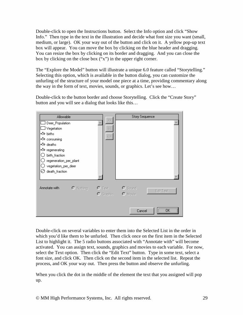
The “Explore the Model” button will illustrate a unique 6.0 feature called “Storytelling.”Selecting this option, which is available in the button dialog, you can customize theunfurling of the structure of your model one piece at a time, providing commentary alongthe way in the form of text, movies, sounds, or graphics. Let’s see how…

Double-click to the button border and choose Storytelling. Click the “Create Story”button and you will see a dialog that looks like this…

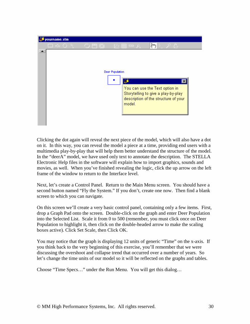
Double-click on several variables to enter them into the Selected List in the order inwhich you’d like them to be unfurled. Then click once on the first item in the SelectedList to highlight it. The 5 radio buttons associated with “Annotate with” will becomeactivated. You can assign text, sounds, graphics and movies to each variable. For now,select the Text option. Then click the “Edit Text” button. Type in some text, select afont size, and click OK. Then click on the second item in the selected list. Repeat theprocess, and OK your way out. Then press the button and observe the unfurling.

When you click the dot in the middle of the element the text that you assigned will popup.


Clicking the dot again will reveal the next piece of the model, which will also have a doton it. In this way, you can reveal the model a piece at a time, providing end users with amultimedia play-by-play that will help them better understand the structure of the model.In the “deerA” model, we have used only text to annotate the description. The STELLAElectronic Help files in the software will explain how to import graphics, sounds andmovies, as well. When you’ve finished revealing the logic, click the up arrow on the leftframe of the window to return to the Interface level.

Next, let’s create a Control Panel. Return to the Main Menu screen. You should have asecond button named “Fly the System.” If you don’t, create one now. Then find a blankscreen to which you can navigate.

On this screen we’ll create a very basic control panel, containing only a few items. First,drop a Graph Pad onto the screen. Double-click on the graph and enter Deer Populationinto the Selected List. Scale it from 0 to 500 (remember, you must click once on DeerPopulation to highlight it, then click on the double-headed arrow to make the scalingboxes active). Click Set Scale, then Click OK.

You may notice that the graph is displaying 12 units of generic “Time” on the x-axis. Ifyou think back to the very beginning of this exercise, you’ll remember that we werediscussing the overshoot and collapse trend that occurred over a number of years. Solet’s change the time units of our model so it will be reflected on the graphs and tables.

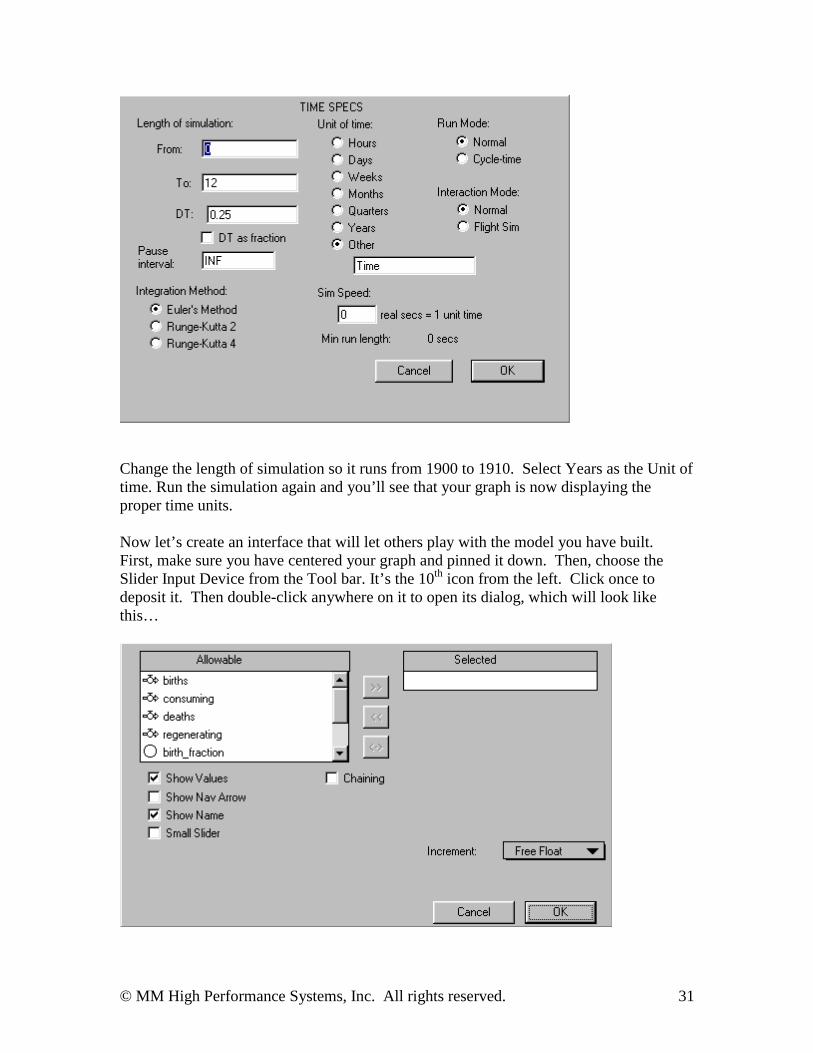
Choose “Time Specs…” under the Run Menu. You will get this dialog…


Change the length of simulation so it runs from 1900 to 1910. Select Years as the Unit oftime. Run the simulation again and you’ll see that your graph is now displaying theproper time units.

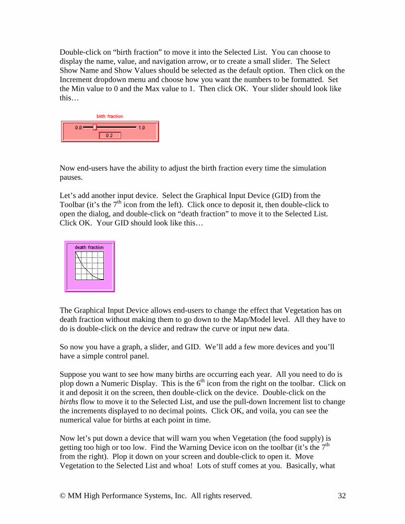
Now let’s create an interface that will let others play with the model you have built.First, make sure you have centered your graph and pinned it down. Then, choose theSlider Input Device from the Tool bar. It’s the 10th icon from the left. Click once todeposit it. Then double-click anywhere on it to open its dialog, which will look likethis…


Double-click on “birth fraction” to move it into the Selected List. You can choose todisplay the name, value, and navigation arrow, or to create a small slider. The SelectShow Name and Show Values should be selected as the default option. Then click on theIncrement dropdown menu and choose how you want the numbers to be formatted. Setthe Min value to 0 and the Max value to 1. Then click OK. Your slider should look likethis…

Now end-users have the ability to adjust the birth fraction every time the simulationpauses.

Let’s add another input device. Select the Graphical Input Device (GID) from theToolbar (it’s the 7th icon from the left). Click once to deposit it, then double-click toopen the dialog, and double-click on “death fraction” to move it to the Selected List.Click OK. Your GID should look like this…

The Graphical Input Device allows end-users to change the effect that Vegetation has ondeath fraction without making them to go down to the Map/Model level. All they have todo is double-click on the device and redraw the curve or input new data.

So now you have a graph, a slider, and GID. We’ll add a few more devices and you’llhave a simple control panel.

Suppose you want to see how many births are occurring each year. All you need to do isplop down a Numeric Display. This is the 6th icon from the right on the toolbar. Click onit and deposit it on the screen, then double-click on the device. Double-click on thebirths flow to move it to the Selected List, and use the pull-down Increment list to changethe increments displayed to no decimal points. Click OK, and voila, you can see thenumerical value for births at each point in time.

Now let’s put down a device that will warn you when Vegetation (the food supply) isgetting too high or too low. Find the Warning Device icon on the toolbar (it’s the 7th

from the right). Plop it down on your screen and double-click to open it. MoveVegetation to the Selected List and whoa! Lots of stuff comes at you. Basically, what


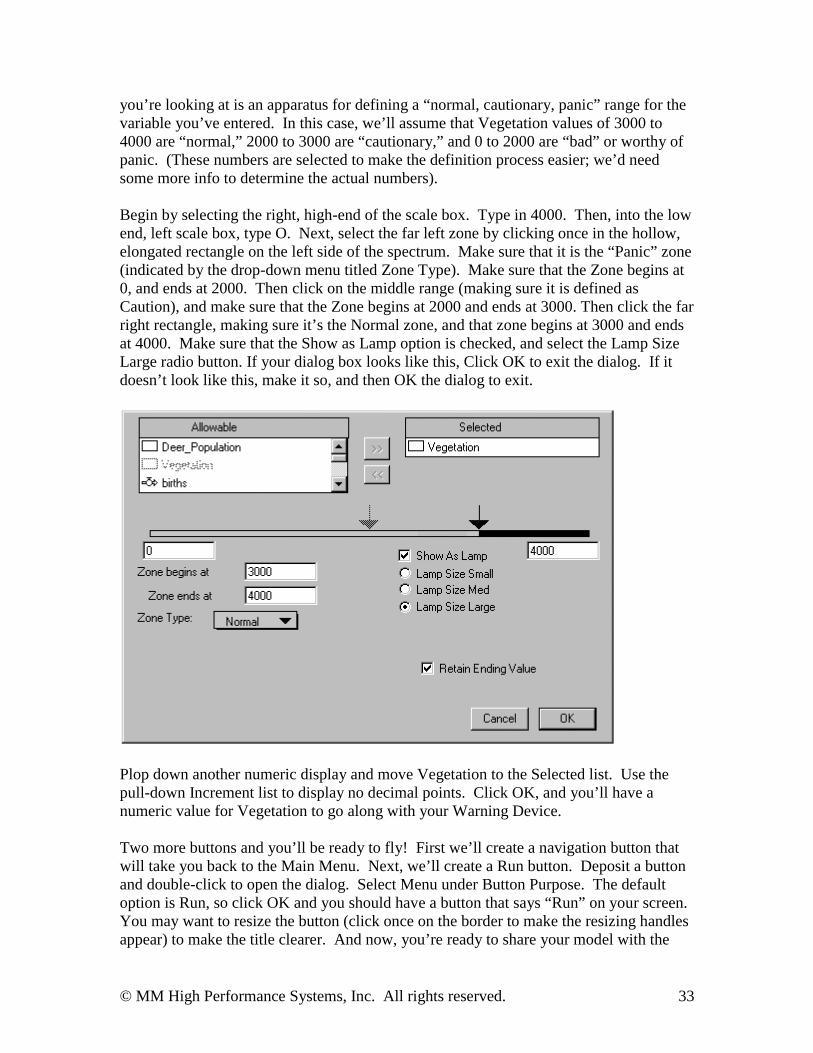
you’re looking at is an apparatus for defining a “normal, cautionary, panic” range for thevariable you’ve entered. In this case, we’ll assume that Vegetation values of 3000 to4000 are “normal,” 2000 to 3000 are “cautionary,” and 0 to 2000 are “bad” or worthy ofpanic. (These numbers are selected to make the definition process easier; we’d needsome more info to determine the actual numbers).

Begin by selecting the right, high-end of the scale box. Type in 4000. Then, into the lowend, left scale box, type O. Next, select the far left zone by clicking once in the hollow,elongated rectangle on the left side of the spectrum. Make sure that it is the “Panic” zone(indicated by the drop-down menu titled Zone Type). Make sure that the Zone begins at0, and ends at 2000. Then click on the middle range (making sure it is defined asCaution), and make sure that the Zone begins at 2000 and ends at 3000. Then click the farright rectangle, making sure it’s the Normal zone, and that zone begins at 3000 and endsat 4000. Make sure that the Show as Lamp option is checked, and select the Lamp SizeLarge radio button. If your dialog box looks like this, Click OK to exit the dialog. If itdoesn’t look like this, make it so, and then OK the dialog to exit.

Plop down another numeric display and move Vegetation to the Selected list. Use thepull-down Increment list to display no decimal points. Click OK, and you’ll have anumeric value for Vegetation to go along with your Warning Device.

Two more buttons and you’ll be ready to fly! First we’ll create a navigation button thatwill take you back to the Main Menu. Next, we’ll create a Run button. Deposit a buttonand double-click to open the dialog. Select Menu under Button Purpose. The defaultoption is Run, so click OK and you should have a button that says “Run” on your screen.You may want to resize the button (click once on the border to make the resizing handlesappear) to make the title clearer. And now, you’re ready to share your model with the


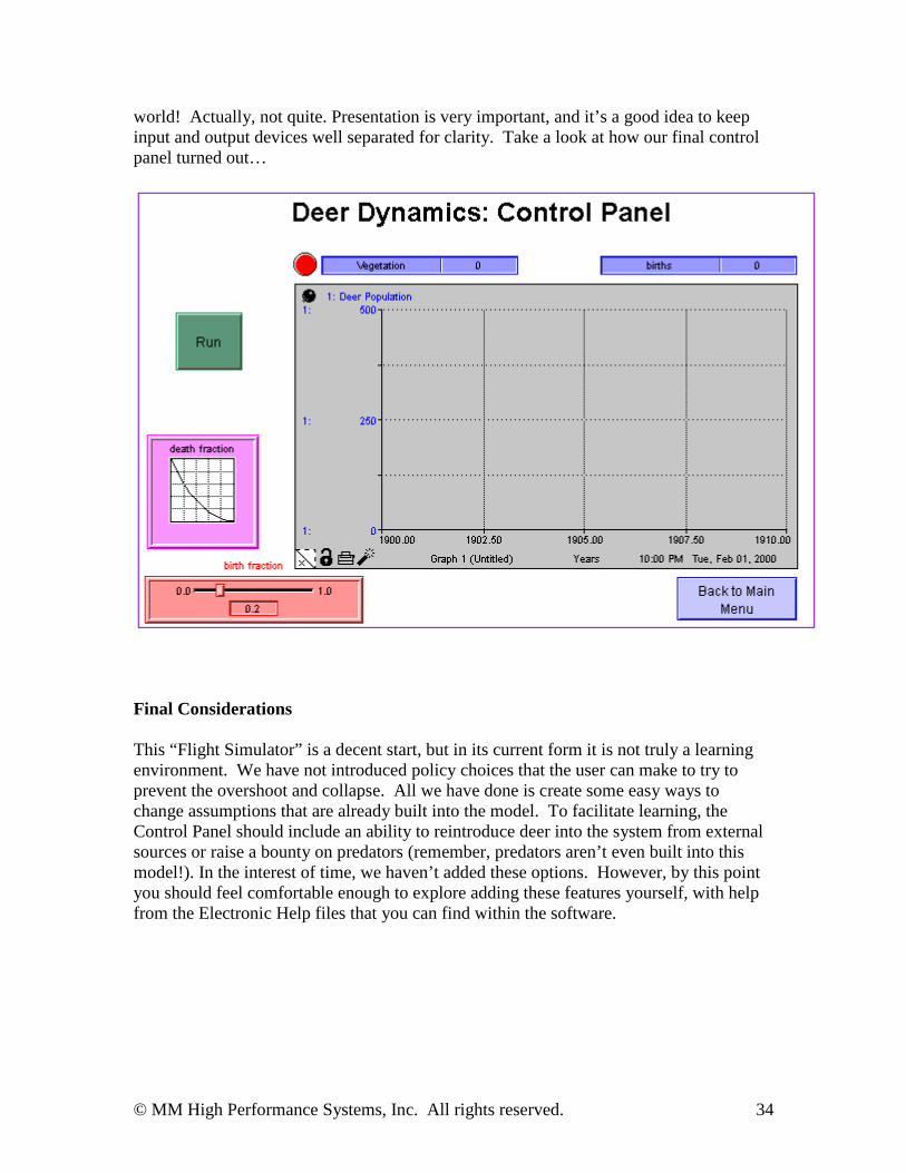
world! Actually, not quite. Presentation is very important, and it’s a good idea to keepinput and output devices well separated for clarity. Take a look at how our final controlpanel turned out…

Final Considerations

This “Flight Simulator” is a decent start, but in its current form it is not truly a learningenvironment. We have not introduced policy choices that the user can make to try toprevent the overshoot and collapse. All we have done is create some easy ways tochange assumptions that are already built into the model. To facilitate learning, theControl Panel should include an ability to reintroduce deer into the system from externalsources or raise a bounty on predators (remember, predators aren’t even built into thismodel!). In the interest of time, we haven’t added these options. However, by this pointyou should feel comfortable enough to explore adding these features yourself, with helpfrom the Electronic Help files that you can find within the software.


This concludes your STELLA “Getting Started” experience. We hope it has given you asense of the incredible power of this highly versatile software tool. If you have anycomments or questions, please contact us via e-mail, fax or phone. We’d love to hearfrom you!

e-mail: [email protected]: 603-643-9636 or 800-332-1202fax: 603-643-9502website: http://www.hps-inc.com

mailto:[email protected]

http://www.hps-inc.com/


Appendix: Basic Software Operations & Features

Rendering

Illustration 1: Depositing, Naming & Re-positioning Stocks & Converters and Nameplates


Illustration 2: Hooking-up Flows


Illustration 3: Re-positioning, “Bending” and Reversing Flows


Illustration 4: Hooking-up and Re-positioning Connectors


Illustration 5: Defining a Graphical Function


SimulatingIllustration 6: Creating a Graph or Table Pad


Illustration 7: Defining a Graph or Table Pad Page


CommunicatingIllustration 8: Using the Text Tool

Documents

Getting Started with STELLA v 6 - Sabancı Üniversitesipeople.sabanciuniv.edu/atilgan/StellaSoft/Guide/STELLA_Guide.pdf · Getting Started with STELLA ... The STELLA software is