Getting Started

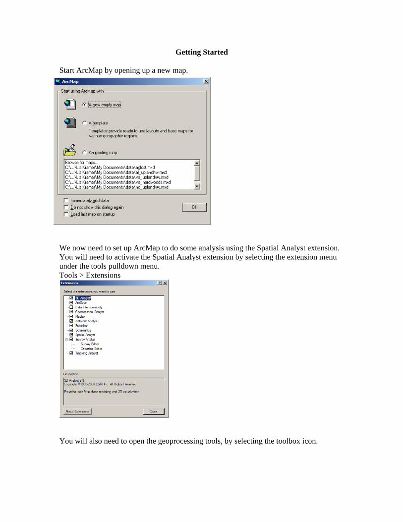
Start ArcMap by opening up a new map.

We now need to set up ArcMap to do some analysis using the Spatial Analyst extension. You will need to activate the Spatial Analyst extension by selecting the extension menu under the tools pulldown menu. Tools > Extensions

You will also need to open the geoprocessing tools, by selecting the toolbox icon.

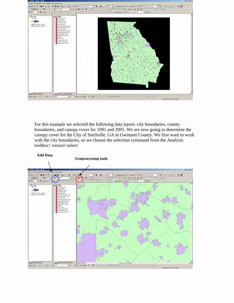
For this example we selected the following data layers: city boundaries, county boundaries, and canopy cover for 1991 and 2005. We are now going to determine the canopy cover for the City of Snellville, GA in Gwinnett County. We first want to work with the city boundaries, so we choose the selection command from the Analysis toolbox> extract>select

Geoprocessing toolsAdd Data

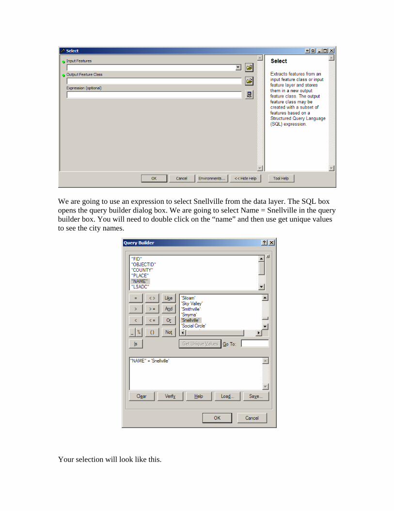
We are going to use an expression to select Snellville from the data layer. The SQL box opens the query builder dialog box. We are going to select Name = Snellville in the query builder box. You will need to double click on the “name” and then use get unique values to see the city names.

Your selection will look like this.

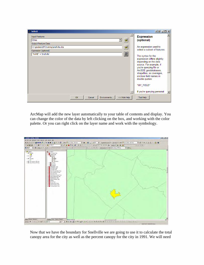
ArcMap will add the new layer automatically to your table of contents and display. You can change the color of the data by left clicking on the box, and working with the color palette. Or you can right click on the layer name and work with the symbology.

Now that we have the boundary for Snellville we are going to use it to calculate the total canopy area for the city as well as the percent canopy for the city in 1991. We will need

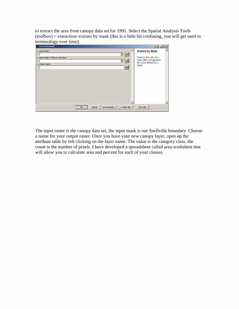
to extract the area from canopy data set for 1991. Select the Spatial Analysis Tools (toolbox) > extraction>extract by mask (this is a little bit confusing, you will get used to terminology over time).

The input raster is the canopy data set, the input mask is our Snellville boundary. Choose a name for your output raster. Once you have your new canopy layer, open up the attribute table by left clicking on the layer name. The value is the category class, the count is the number of pixels. I have developed a spreadsheet called area worksheet that will allow you to calculate area and percent for each of your classes.

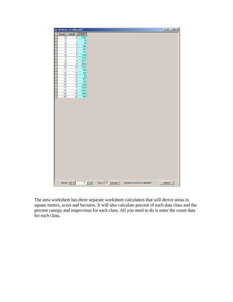
The area worksheet has three separate worksheet calculators that will derive areas in square meters, acres and hectares. It will also calculate percent of each data class and the percent canopy and impervious for each class. All you need to do is enter the count data for each class.

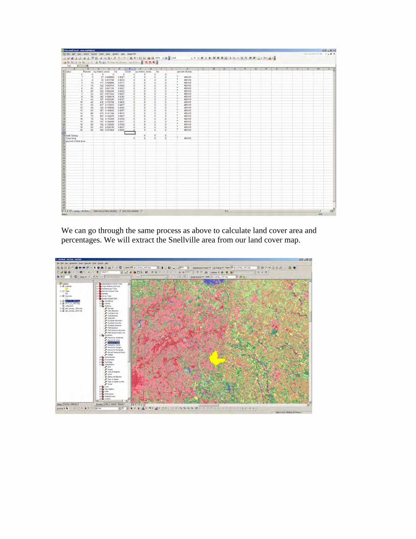
We can go through the same process as above to calculate land cover area and percentages. We will extract the Snellville area from our land cover map.

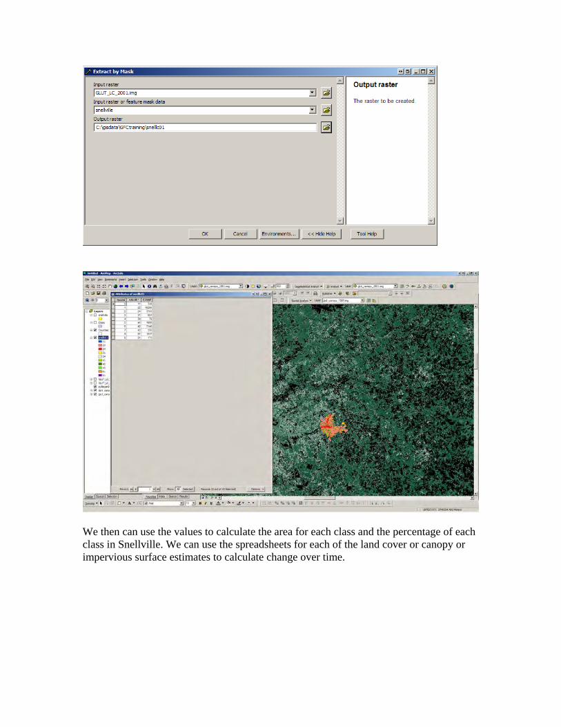
We then can use the values to calculate the area for each class and the percentage of each class in Snellville. We can use the spreadsheets for each of the land cover or canopy or impervious surface estimates to calculate change over time.

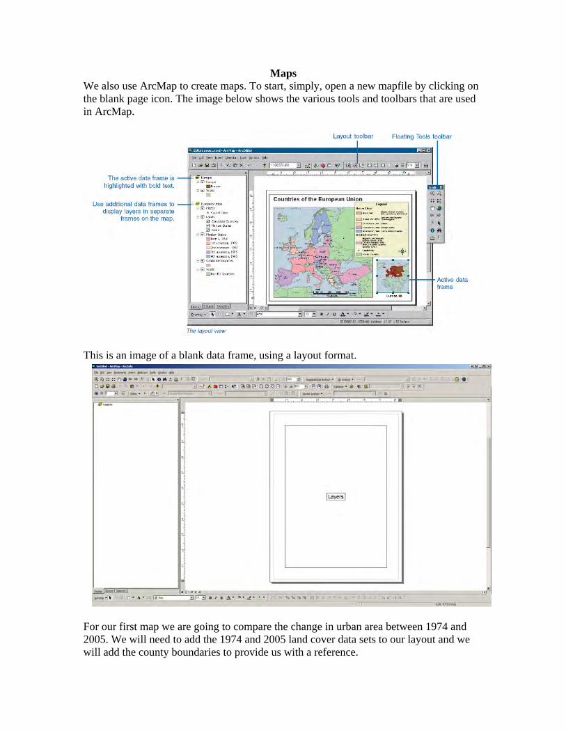
Maps We also use ArcMap to create maps. To start, simply, open a new mapfile by clicking on the blank page icon. The image below shows the various tools and toolbars that are used in ArcMap.

This is an image of a blank data frame, using a layout format.

For our first map we are going to compare the change in urban area between 1974 and 2005. We will need to add the 1974 and 2005 land cover data sets to our layout and we will add the county boundaries to provide us with a reference.

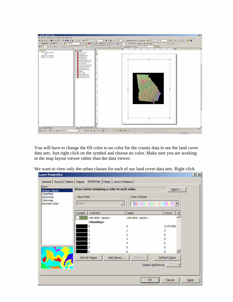
You will have to change the fill color to no color for the county data to see the land cover data sets. Just right click on the symbol and choose no color. Make sure you are working in the map layout viewer rather than the data viewer. We want to view only the urban classes for each of our land cover data sets. Right click

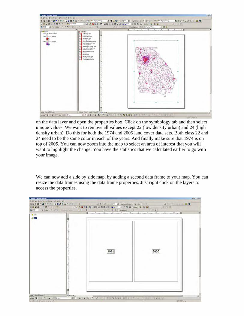
on the data layer and open the properties box. Click on the symbology tab and then select unique values. We want to remove all values except 22 (low density urban) and 24 (high density urban). Do this for both the 1974 and 2005 land cover data sets. Both class 22 and 24 need to be the same color in each of the years. And finally make sure that 1974 is on top of 2005. You can now zoom into the map to select an area of interest that you will want to highlight the change. You have the statistics that we calculated earlier to go with your image. We can now add a side by side map, by adding a second data frame to your map. You can resize the data frames using the data frame properties. Just right click on the layers to access the properties.

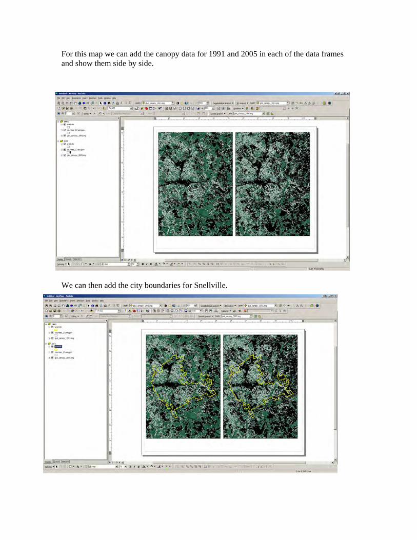
For this map we can add the canopy data for 1991 and 2005 in each of the data frames and show them side by side.

We can then add the city boundaries for Snellville.

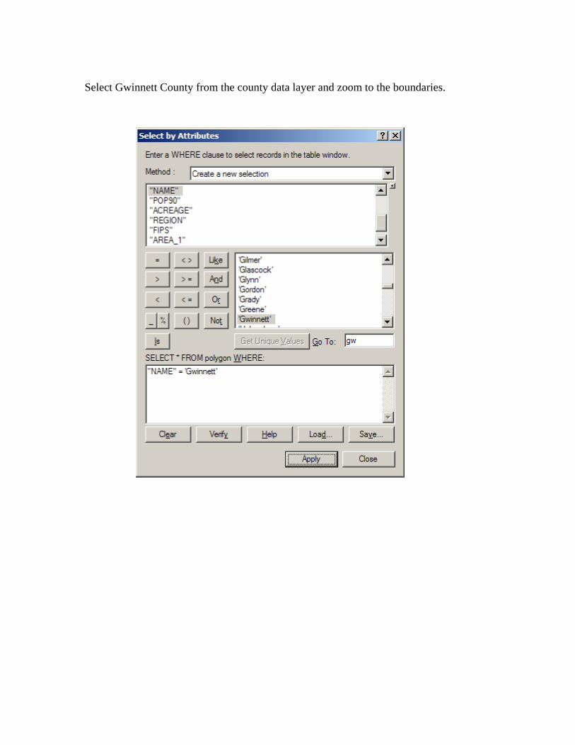
Select Gwinnett County from the county data layer and zoom to the boundaries.

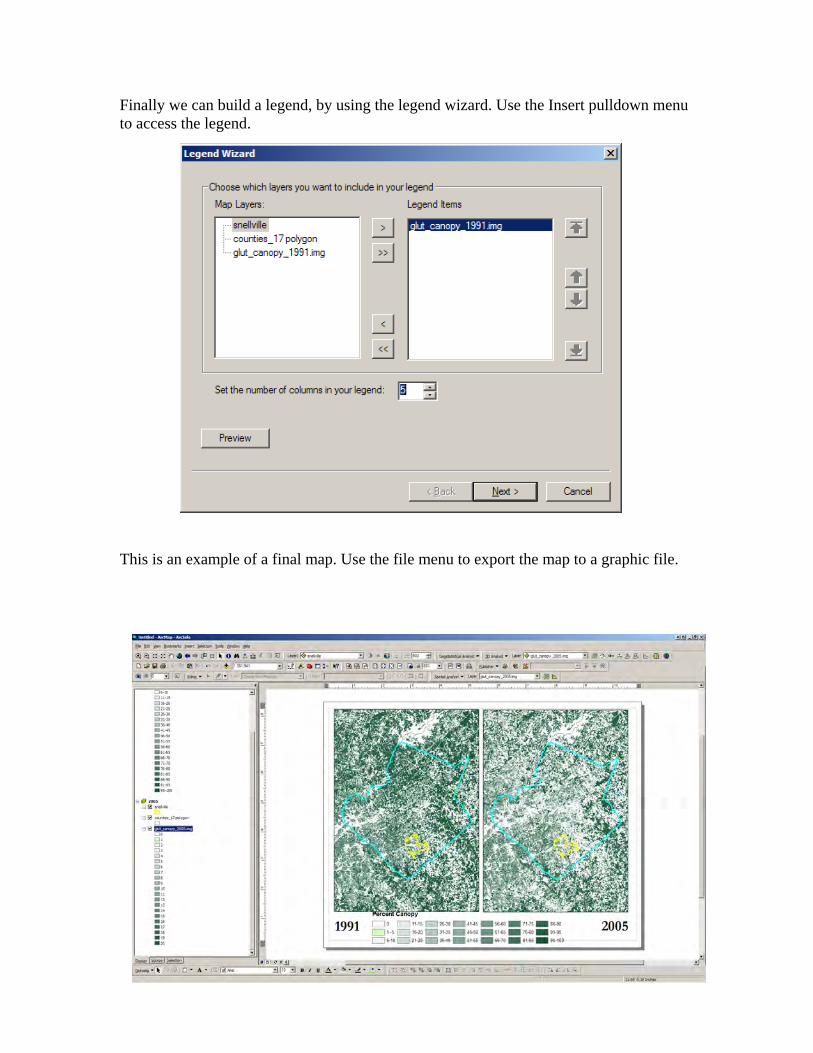
Finally we can build a legend, by using the legend wizard. Use the Insert pulldown menu to access the legend.

This is an example of a final map. Use the file menu to export the map to a graphic file.