Getting Started in Frequencies, Crosstab, Factor and Regression Analysis

(ver. 2.0 beta, draft)

Oscar Torres-ReynaData Consultantotorres@princeton.edu

http://dss.princeton.edu/training/

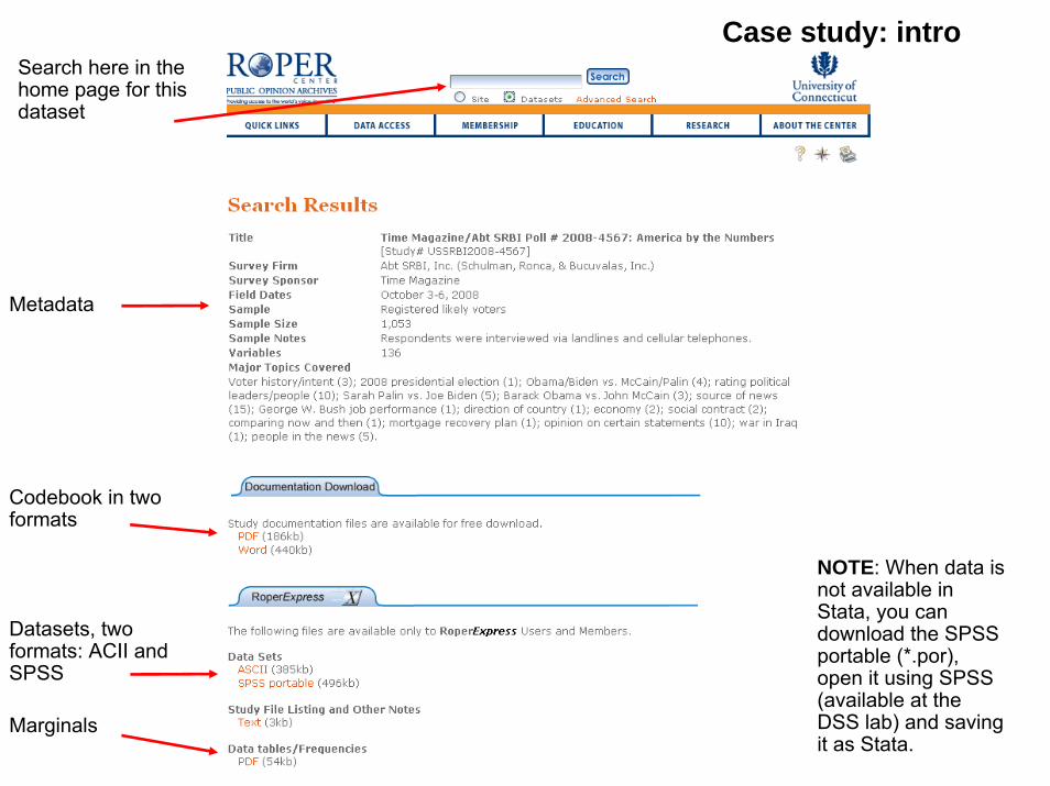
Case study: introSearch here in the home page for this dataset

Codebook in two formats

Datasets, two formats: ACII and SPSS

Marginals

Metadata

NOTE: When data is not available in Stata, you can download the SPSS portable (*.por), open it using SPSS (available at the DSS lab) and saving it as Stata.

Total 1,053 100.00 Female 552.611604 52.48 100.00 Male 500.388396 47.52 47.52 ASK) Freq. Percent Cum. (DO NOT A. Gender

. tab qa [aweight=weight] /*With weights*/

.

Total 1,053 100.00 Female 560 53.18 100.00 Male 493 46.82 46.82 ASK) Freq. Percent Cum. (DO NOT A. Gender

. tab qa /*No weights*/

.

Total 1,053 100.00 (VOL) Undecided/Don't know/no answer 78.61762284 7.47 100.00 (VOL) Other/Neither 20.5570831 1.95 92.53John McCain and Sarah Palin, the Republ 449.487545 42.69 90.58Barack Obama and Joe Biden, the Democra 504.337749 47.90 47.90 Barack Freq. Percent Cum. held today and the candidates were Q5. If the Presidential election were

. tab q5 [aweight=weight] /*With weights*/

.

Total 1,053 100.00 (VOL) Undecided/Don't know/no answer 87 8.26 100.00 (VOL) Other/Neither 21 1.99 91.74John McCain and Sarah Palin, the Republ 464 44.06 89.74Barack Obama and Joe Biden, the Democra 481 45.68 45.68 Barack Freq. Percent Cum. held today and the candidates were Q5. If the Presidential election were

. tab q5 /*No weights*/

Case study: frequenciesDistribution of electoral preferences and gender. According to the codebook ‘q5’ has the electoral question and ‘qa’ gender.

NOTE: At this point, it is strongly recommended to open a log to keep a record of your work and to extract output, type:

log using mywork.log

You could also open a do-file by typingdoedit and copy your commands there.

No weights

Using weights

No weights

Using weights

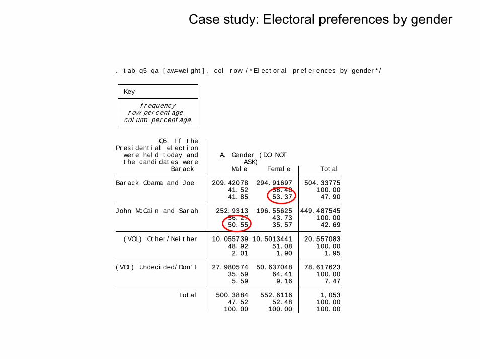
100.00 100.00 100.00 47.52 52.48 100.00 Total 500.3884 552.6116 1,053 5.59 9.16 7.47 35.59 64.41 100.00 (VOL) Undecided/Don't 27.980574 50.637048 78.617623 2.01 1.90 1.95 48.92 51.08 100.00 (VOL) Other/Neither 10.055739 10.5013441 20.557083 50.55 35.57 42.69 56.27 43.73 100.00 John McCain and Sarah 252.9313 196.55625 449.487545 41.85 53.37 47.90 41.52 58.48 100.00 Barack Obama and Joe 209.42078 294.91697 504.33775 Barack Male Female Total the candidates were ASK) were held today and A. Gender (DO NOTPresidential election Q5. If the

column percentage row percentage frequency Key

. tab q5 qa [aw=weight], col row /*Electoral preferences by gender*/

Case study: Electoral preferences by gender

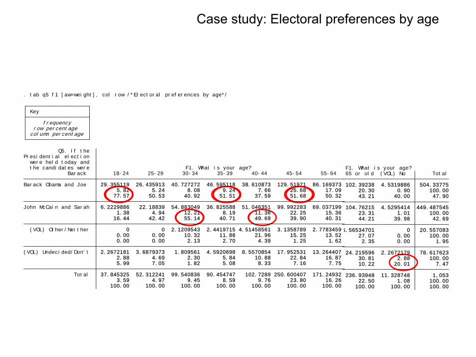
Case study: Electoral preferences by age

100.00 100.00 100.00 100.00 100.00 100.00 100.00 3.59 4.97 9.45 8.59 9.76 23.80 16.26 Total 37.845325 52.312241 99.540836 90.454747 102.7289 250.600407 171.24932 5.99 7.05 1.82 5.08 8.33 7.16 7.75 2.88 4.69 2.30 5.84 10.88 22.84 16.87 (VOL) Undecided/Don't 2.2672181 3.6879373 1.809561 4.5920698 8.5570854 17.952531 13.264407 0.00 0.00 2.13 2.70 4.39 1.25 1.62 0.00 0.00 10.32 11.88 21.96 15.25 13.52 (VOL) Other/Neither 0 0 2.1209543 2.4419715 4.51458561 3.1358789 2.7783459 16.44 42.42 55.14 40.71 49.69 39.90 40.31 1.38 4.94 12.21 8.19 11.36 22.25 15.36 John McCain and Sarah 6.2229886 22.18839 54.883049 36.825588 51.046351 99.992283 69.037199 77.57 50.53 40.92 51.51 37.59 51.68 50.32 5.82 5.24 8.08 9.24 7.66 25.68 17.09 Barack Obama and Joe 29.355119 26.435913 40.727272 46.595118 38.610873 129.51971 86.169373 Barack 18-24 25-29 30-34 35-39 40-44 45-54 55-64 the candidates were F1. What is your age? were held today and Presidential election Q5. If the

column percentage row percentage frequency Key

. tab q5 f1 [aw=weight], col row /*Electoral preferences by age*/

100.00 100.00 100.00 22.50 1.08 100.00 236.93948 11.328748 1,053 10.22 20.01 7.47 30.81 2.88 100.00 24.219596 2.2672179 78.617623 2.35 0.00 1.95 27.07 0.00 100.00 5.56534701 0 20.557083 44.21 39.98 42.69 23.31 1.01 100.00 104.76215 4.5295414 449.487545 43.21 40.00 47.90 20.30 0.90 100.00 102.39238 4.5319886 504.33775 65 or old (VOL) No Total F1. What is your age?

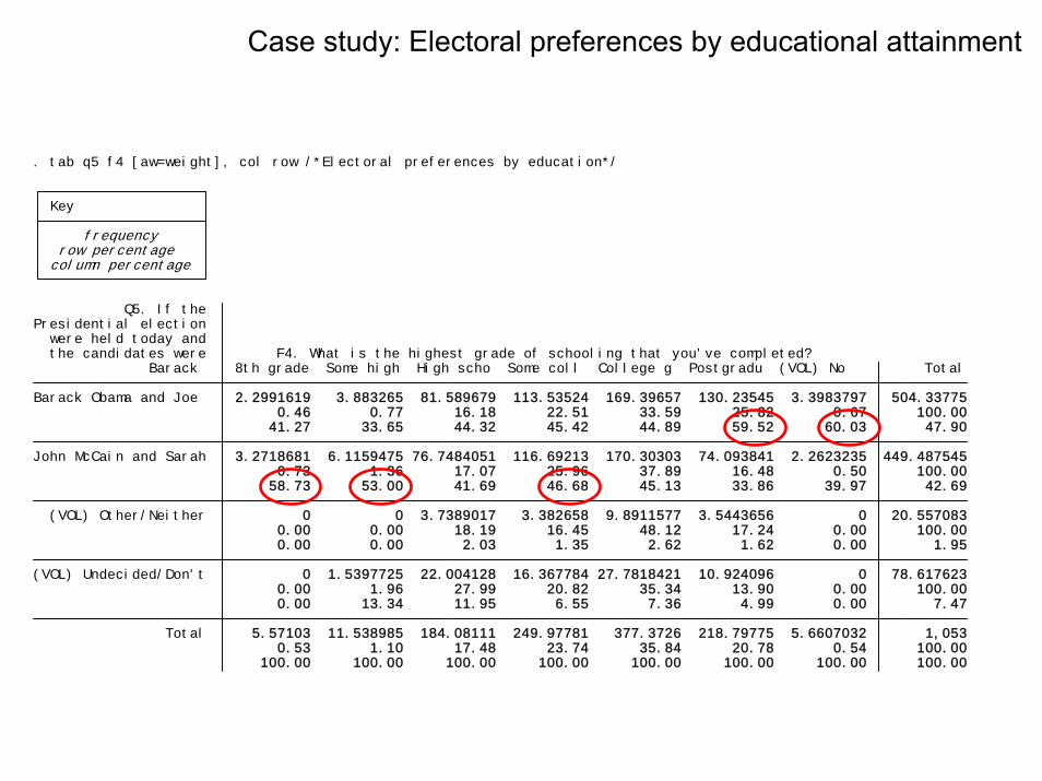
100.00 100.00 100.00 100.00 100.00 100.00 100.00 100.00 0.53 1.10 17.48 23.74 35.84 20.78 0.54 100.00 Total 5.57103 11.538985 184.08111 249.97781 377.3726 218.79775 5.6607032 1,053 0.00 13.34 11.95 6.55 7.36 4.99 0.00 7.47 0.00 1.96 27.99 20.82 35.34 13.90 0.00 100.00 (VOL) Undecided/Don't 0 1.5397725 22.004128 16.367784 27.7818421 10.924096 0 78.617623 0.00 0.00 2.03 1.35 2.62 1.62 0.00 1.95 0.00 0.00 18.19 16.45 48.12 17.24 0.00 100.00 (VOL) Other/Neither 0 0 3.7389017 3.382658 9.8911577 3.5443656 0 20.557083 58.73 53.00 41.69 46.68 45.13 33.86 39.97 42.69 0.73 1.36 17.07 25.96 37.89 16.48 0.50 100.00 John McCain and Sarah 3.2718681 6.1159475 76.7484051 116.69213 170.30303 74.093841 2.2623235 449.487545 41.27 33.65 44.32 45.42 44.89 59.52 60.03 47.90 0.46 0.77 16.18 22.51 33.59 25.82 0.67 100.00 Barack Obama and Joe 2.2991619 3.883265 81.589679 113.53524 169.39657 130.23545 3.3983797 504.33775 Barack 8th grade Some high High scho Some coll College g Postgradu (VOL) No Total the candidates were F4. What is the highest grade of schooling that you've completed? were held today and Presidential election Q5. If the

column percentage row percentage frequency Key

. tab q5 f4 [aw=weight], col row /*Electoral preferences by education*/

Case study: Electoral preferences by educational attainment

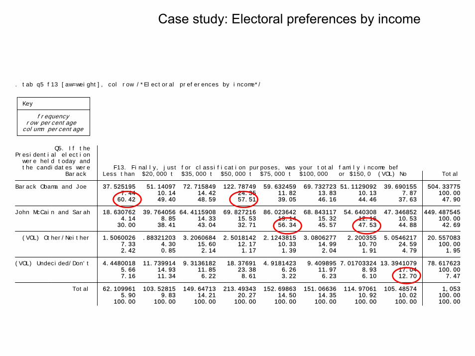
100.00 100.00 100.00 100.00 100.00 100.00 100.00 100.00 100.00 5.90 9.83 14.21 20.27 14.50 14.35 10.92 10.02 100.00 Total 62.109961 103.52815 149.64713 213.49343 152.69863 151.06636 114.97061 105.48574 1,053 7.16 11.34 6.22 8.61 3.22 6.23 6.10 12.70 7.47 5.66 14.93 11.85 23.38 6.26 11.97 8.93 17.04 100.00 (VOL) Undecided/Don't 4.4480018 11.739914 9.3136182 18.37691 4.9181423 9.409895 7.01703324 13.3941079 78.617623 2.42 0.85 2.14 1.17 1.39 2.04 1.91 4.79 1.95 7.33 4.30 15.60 12.17 10.33 14.99 10.70 24.59 100.00 (VOL) Other/Neither 1.5060026 .88321203 3.2060684 2.5018142 2.1243815 3.0806277 2.200355 5.0546217 20.557083 30.00 38.41 43.04 32.71 56.34 45.57 47.53 44.88 42.69 4.14 8.85 14.33 15.53 19.14 15.32 12.16 10.53 100.00 John McCain and Sarah 18.630762 39.764056 64.4115908 69.827216 86.023642 68.843117 54.640308 47.346852 449.487545 60.42 49.40 48.59 57.51 39.05 46.16 44.46 37.63 47.90 7.44 10.14 14.42 24.35 11.82 13.83 10.13 7.87 100.00 Barack Obama and Joe 37.525195 51.14097 72.715849 122.78749 59.632459 69.732723 51.1129092 39.690155 504.33775 Barack Less than $20,000 t $35,000 t $50,000 t $75,000 t $100,000 or $150,0 (VOL) No Total the candidates were F13. Finally, just for classification purposes, was your total family income bef were held today and Presidential election Q5. If the

column percentage row percentage frequency Key

. tab q5 f13 [aw=weight], col row /*Electoral preferences by income*/

Case study: Electoral preferences by income

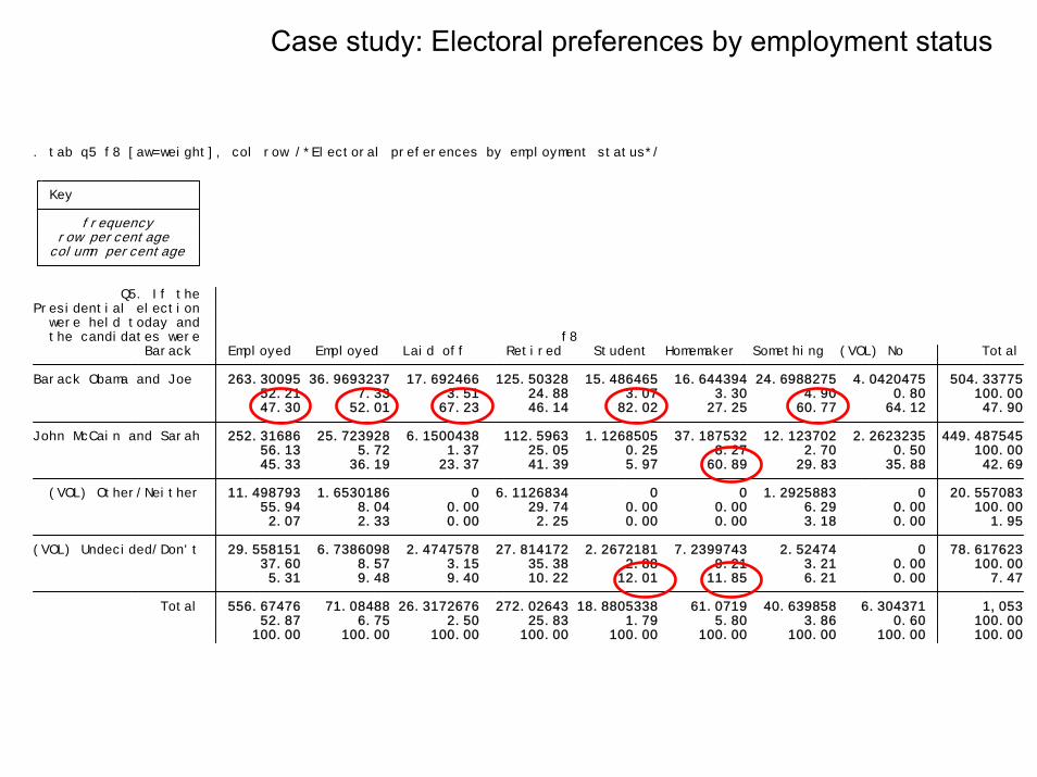
100.00 100.00 100.00 100.00 100.00 100.00 100.00 100.00 100.00 52.87 6.75 2.50 25.83 1.79 5.80 3.86 0.60 100.00 Total 556.67476 71.08488 26.3172676 272.02643 18.8805338 61.0719 40.639858 6.304371 1,053 5.31 9.48 9.40 10.22 12.01 11.85 6.21 0.00 7.47 37.60 8.57 3.15 35.38 2.88 9.21 3.21 0.00 100.00 (VOL) Undecided/Don't 29.558151 6.7386098 2.4747578 27.814172 2.2672181 7.2399743 2.52474 0 78.617623 2.07 2.33 0.00 2.25 0.00 0.00 3.18 0.00 1.95 55.94 8.04 0.00 29.74 0.00 0.00 6.29 0.00 100.00 (VOL) Other/Neither 11.498793 1.6530186 0 6.1126834 0 0 1.2925883 0 20.557083 45.33 36.19 23.37 41.39 5.97 60.89 29.83 35.88 42.69 56.13 5.72 1.37 25.05 0.25 8.27 2.70 0.50 100.00 John McCain and Sarah 252.31686 25.723928 6.1500438 112.5963 1.1268505 37.187532 12.123702 2.2623235 449.487545 47.30 52.01 67.23 46.14 82.02 27.25 60.77 64.12 47.90 52.21 7.33 3.51 24.88 3.07 3.30 4.90 0.80 100.00 Barack Obama and Joe 263.30095 36.9693237 17.692466 125.50328 15.486465 16.644394 24.6988275 4.0420475 504.33775 Barack Employed Employed Laid off Retired Student Homemaker Something (VOL) No Total the candidates were f8 were held today and Presidential election Q5. If the

column percentage row percentage frequency Key

. tab q5 f8 [aw=weight], col row /*Electoral preferences by employment status*/

Case study: Electoral preferences by employment status

Case study: Testing for associations (preparing the data)Before running any test we need to prepare the data by setting to missing any non-valid response (like “don’t know/no answer/not sure”) unless is relevant to the question. It is important to ‘clean’ the variables for the tests to be as accurate as possible. For demographics we will remove non-response items. Here are a series of commands per variable (columns) to prepare some variables for you to run on your own.

Description Age Education Income Employment Gender

creating a new variable gen age=f1 gen educ=f4 gen income=f13 gen employ=f8 gen gender=qa

exploring the new variable tab age tab educ tab income tab employ tab gender

checking for labels from original variable labelbook f1 labelbook f4 labelbook f13 labelbook f8 labelbook qa

assigning labels to new variable label value age f1 label value educ f4 label value income f13 label value employ f8 label value

gender qa

exploring the new variable tab age tab educ tab income tab employ tab gender

setting no response to missing

replace age=. if age>8 replace educ=. if educ==8 replace income=. if

income==8 replace employ=. if employ==8

adding variable labels label variable age "Age"

label variable educ "Educational attainment"

label variable income "Family income"

label variable employ "Employment status"

exploring the new variable tab age tab educ tab income tab employ

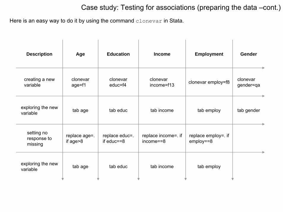
Case study: Testing for associations (preparing the data –cont.)

Here is an easy way to do it by using the command clonevar in Stata.

Description Age Education Income Employment Gender

creating a new variable

clonevarage=f1

clonevareduc=f4

clonevarincome=f13 clonevar employ=f8 clonevar

gender=qa

exploring the new variable tab age tab educ tab income tab employ tab gender

setting no response to missing

replace age=. if age>8

replace educ=. if educ==8

replace income=. if income==8

replace employ=. if employ==8

exploring the new variable tab age tab educ tab income tab employ

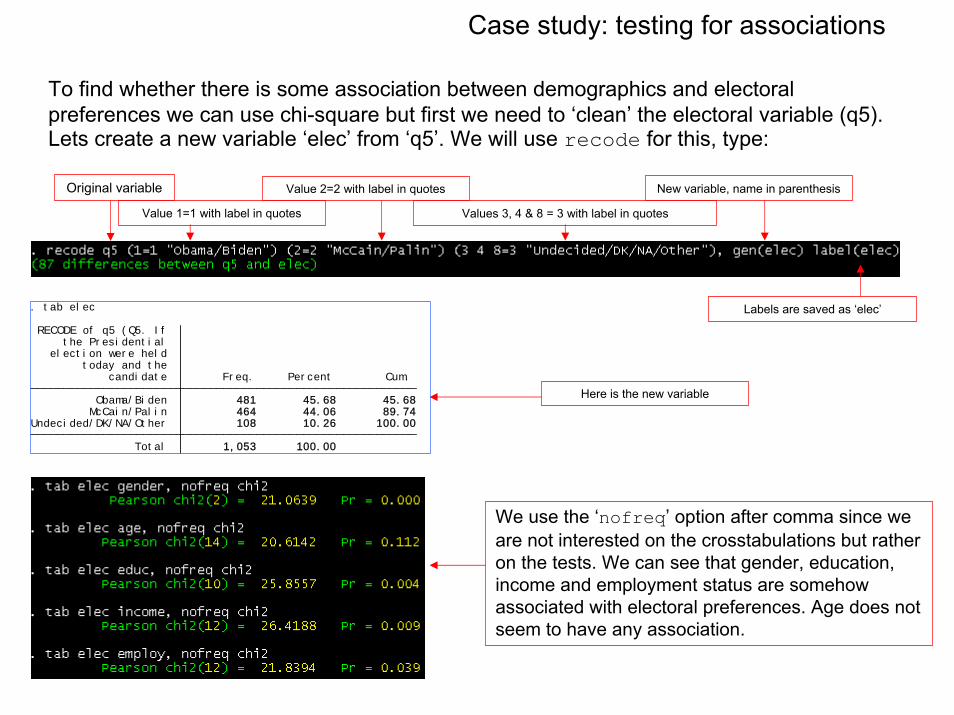
Case study: testing for associations

To find whether there is some association between demographics and electoral preferences we can use chi-square but first we need to ‘clean’ the electoral variable (q5).Lets create a new variable ‘elec’ from ‘q5’. We will use recode for this, type:

Original variable

Value 1=1 with label in quotes

Value 2=2 with label in quotes

Values 3, 4 & 8 = 3 with label in quotes

New variable, name in parenthesis

Labels are saved as ‘elec’

Here is the new variable

We use the ‘nofreq’ option after comma since we are not interested on the crosstabulations but rather on the tests. We can see that gender, education, income and employment status are somehow associated with electoral preferences. Age does not seem to have any association.

Total 1,053 100.00 Undecided/DK/NA/Other 108 10.26 100.00 McCain/Palin 464 44.06 89.74 Obama/Biden 481 45.68 45.68 candidate Freq. Percent Cum. today and the election were held the Presidential RECODE of q5 (Q5. If

. tab elec

Case study: descriptive statistics

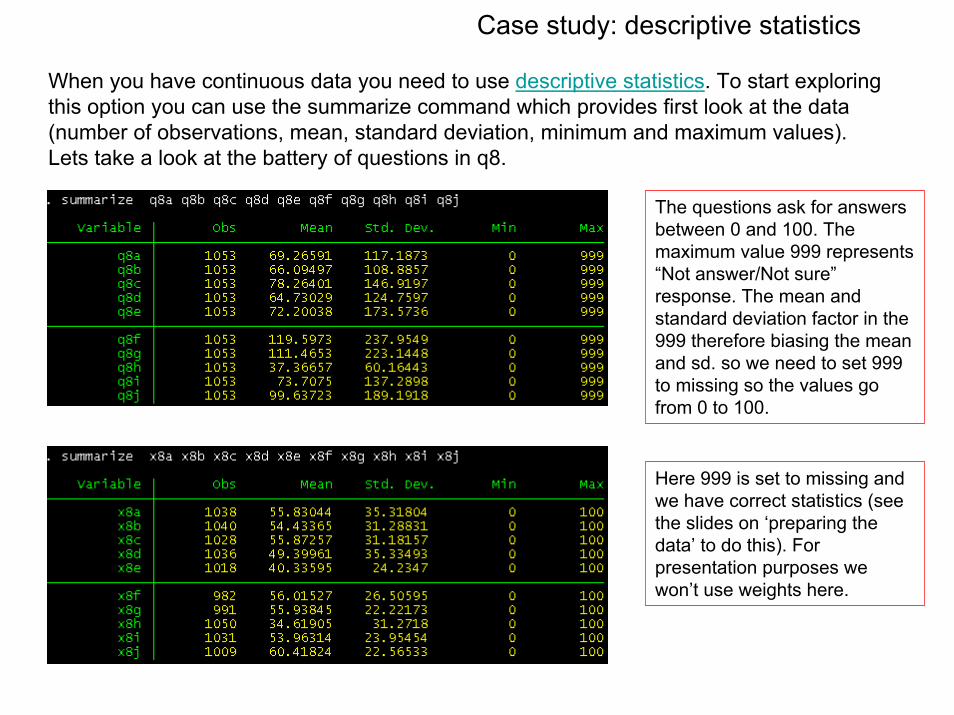
When you have continuous data you need to use descriptive statistics. To start exploring this option you can use the summarize command which provides first look at the data (number of observations, mean, standard deviation, minimum and maximum values). Lets take a look at the battery of questions in q8.

The questions ask for answers between 0 and 100. The maximum value 999 represents “Not answer/Not sure”response. The mean and standard deviation factor in the 999 therefore biasing the mean and sd. so we need to set 999 to missing so the values go from 0 to 100.

Here 999 is set to missing and we have correct statistics (see the slides on ‘preparing the data’ to do this). For presentation purposes we won’t use weights here.

Case study: descriptive statistics

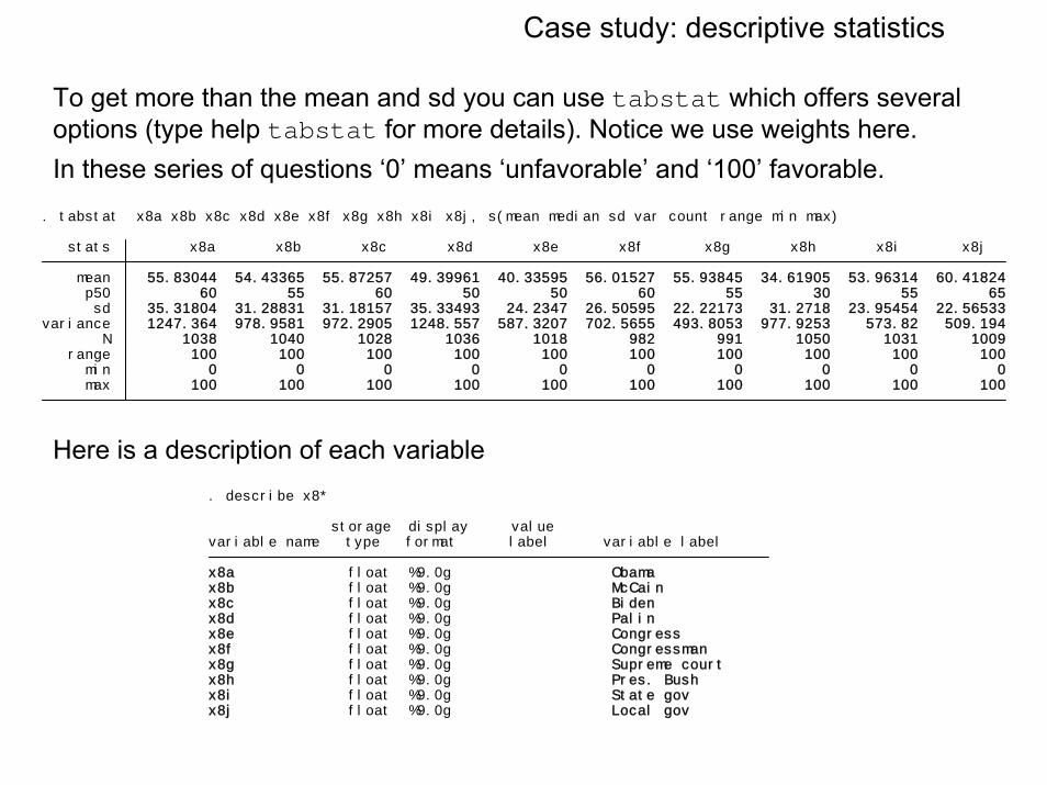
To get more than the mean and sd you can use tabstat which offers several options (type help tabstat for more details). Notice we use weights here.In these series of questions ‘0’ means ‘unfavorable’ and ‘100’ favorable.

Here is a description of each variable

max 100 100 100 100 100 100 100 100 100 100 min 0 0 0 0 0 0 0 0 0 0 range 100 100 100 100 100 100 100 100 100 100 N 1038 1040 1028 1036 1018 982 991 1050 1031 1009variance 1247.364 978.9581 972.2905 1248.557 587.3207 702.5655 493.8053 977.9253 573.82 509.194 sd 35.31804 31.28831 31.18157 35.33493 24.2347 26.50595 22.22173 31.2718 23.95454 22.56533 p50 60 55 60 50 50 60 55 30 55 65 mean 55.83044 54.43365 55.87257 49.39961 40.33595 56.01527 55.93845 34.61905 53.96314 60.41824 stats x8a x8b x8c x8d x8e x8f x8g x8h x8i x8j

. tabstat x8a x8b x8c x8d x8e x8f x8g x8h x8i x8j, s(mean median sd var count range min max)

x8j float %9.0g Local govx8i float %9.0g State govx8h float %9.0g Pres. Bushx8g float %9.0g Supreme courtx8f float %9.0g Congressmanx8e float %9.0g Congressx8d float %9.0g Palinx8c float %9.0g Bidenx8b float %9.0g McCainx8a float %9.0g Obama variable name type format label variable label storage display value

. describe x8*

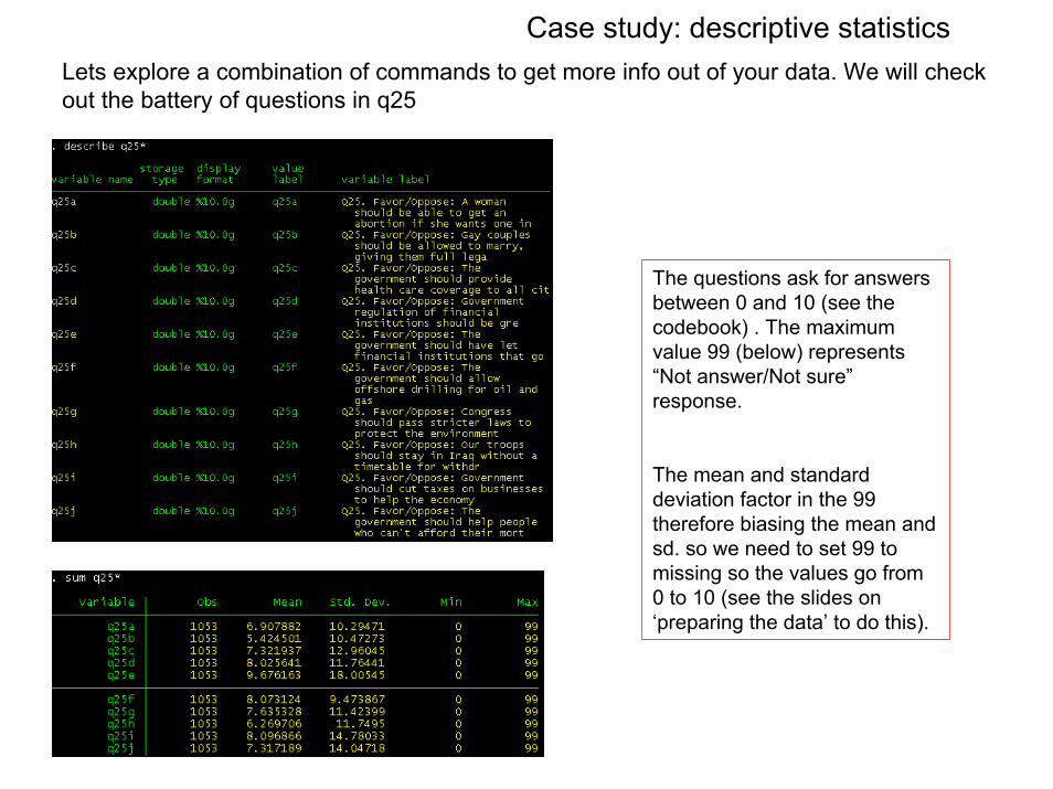
Case study: descriptive statisticsLets explore a combination of commands to get more info out of your data. We will check out the battery of questions in q25

The questions ask for answers between 0 and 10 (see the codebook) . The maximum value 99 (below) represents “Not answer/Not sure”response.

The mean and standard deviation factor in the 99 therefore biasing the mean and sd. so we need to set 99 to missing so the values go from 0 to 10 (see the slides on ‘preparing the data’ to do this).

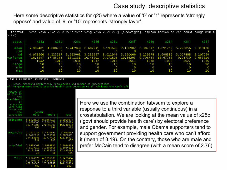
Case study: descriptive statisticsHere some descriptive statistics for q25 where a value of ‘0’ or ’1’ represents ‘strongly oppose’ and value of ‘9’ or ’10’ represents ‘strongly favor’.

Here we use the combination tab/sum to explore a response to a third variable (usually continuous) in a crosstabulation. We are looking at the mean value of x25c (‘govt should provide health care’) by electoral preference and gender. For example, male Obama supporters tend to support government providing health care who can’t afford it (mean of 8.19). On the contrary, those who are male and prefer McCain tend to disagree (with a mean score of 2.76)

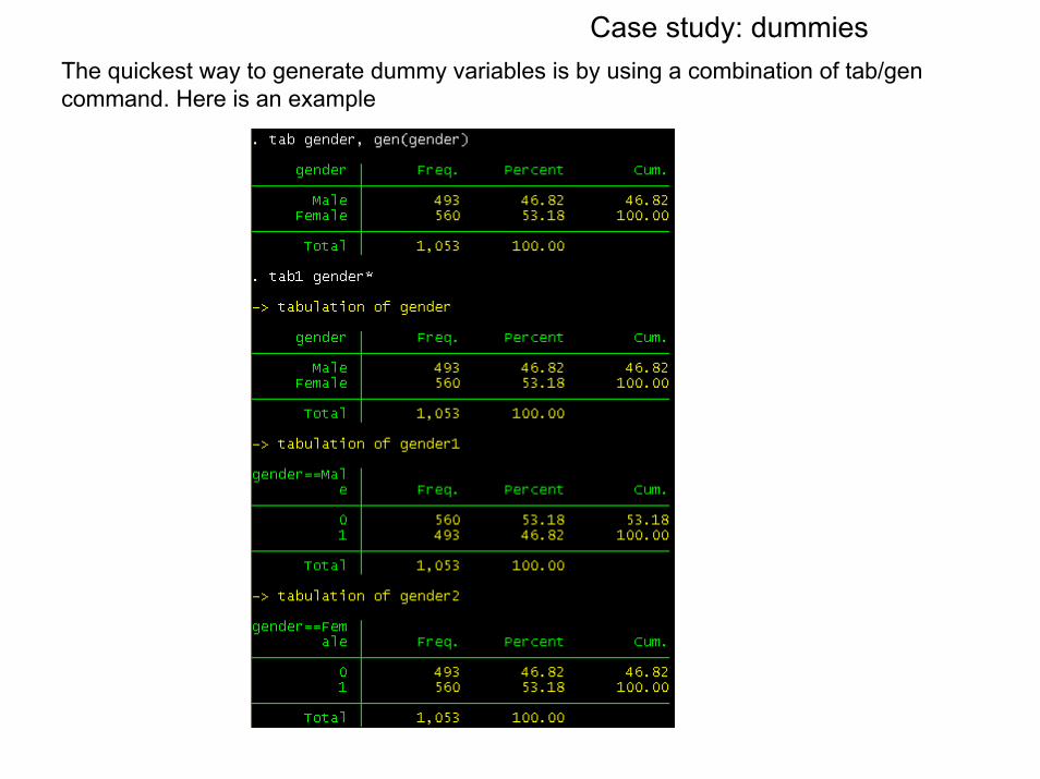
Case study: dummiesThe quickest way to generate dummy variables is by using a combination of tab/gen command. Here is an example

Case study: factor analysisFactor analysis is a data reduction technique. Question 8 has a battery of questions evaluating favorability levels for different candidates/politicians

x8j -0.0425 0.6554 0.5686 x8i -0.0373 0.7252 0.4728 x8h 0.8225 0.2936 0.2373 x8g 0.2197 0.5555 0.6432 x8f -0.1691 0.6717 0.5202 x8e -0.4759 0.5533 0.4674 x8d 0.9180 0.1434 0.1367 x8c -0.8531 0.1799 0.2399 x8b 0.8586 0.2150 0.2165 x8a -0.9046 0.1045 0.1709 Variable Factor1 Factor2 Uniqueness

Factor loadings (pattern matrix) and unique variances

LR test: independent vs. saturated: chi2( 45) = 4884.51 Prob>chi2 = 0.0000 Factor10 0.14031 . 0.0140 1.0000 Factor9 0.15591 0.01559 0.0156 0.9860 Factor8 0.27398 0.11808 0.0274 0.9704 Factor7 0.39262 0.11864 0.0393 0.9430 Factor6 0.53172 0.13910 0.0532 0.9037 Factor5 0.58340 0.05168 0.0583 0.8505 Factor4 0.73671 0.15331 0.0737 0.7922 Factor3 0.85870 0.12199 0.0859 0.7185 Factor2 2.21756 1.35886 0.2218 0.6327 Factor1 4.10910 1.89154 0.4109 0.4109 Factor Eigenvalue Difference Proportion Cumulative

Rotation: (unrotated) Number of params = 19 Method: principal-component factors Retained factors = 2Factor analysis/correlation Number of obs = 897

(obs=897). factor x8a x8b x8c x8d x8e x8f x8g x8h x8i x8j, pcf

Principal-components factoringVariables

Total variance accounted by each factor. The sum of all eigenvalues = total number of variables. When negative, the sum of eigenvalues = total number of factors (variables) with positive eigenvalues.Kaiser criterion suggests to retain those factors with eigenvalues equal or higher than 1.

Difference between one eigenvalue and the next.

Since the sum of eigenvalues= total number of variables. Proportion indicate the relative weight of each factor in the total variance. For example, 4.109/10=0.4109. The first factor explains 41% of the total variance

Cumulative shows the amount of variance explained by n+(n-1) factors. For example, factor 1 and factor 2 account for 63% of the total variance.

Factor loadings are the weights and correlations between each variable and the factor. The higher the load the more relevant in defining the factor’s conceptual meaning. A negative value indicates an inverse impact on the factor. Here, two factors are retained because both have eigenvalues over 1. It seems that ‘x8b’, ‘x8d’ and ‘x8h’ define factor1, and ‘x8f’, and ‘x8i’ define factor2.

Uniqueness is the variance that is ‘unique’to the variable and not shared with other variables. It is equal to 1 – communality (variance that is shared with other variables). For example, 64% of the variance in ‘x8g’ is not share with other variables in the overall factor model. On the contrary ‘x8a’ has low variance not accounted by other variables (17%). Notice that the greater ‘uniqueness’ the lower the relevance of the variable in the factor model.

Case study: factor analysis

Factor analysis is a data reduction technique. Question 8 has a battery of questions evaluating favorability levels for different candidates/politicians

Factor2 0.1177 0.9930 Factor1 0.9930 -0.1177 Factor1 Factor2

Factor rotation matrix

x8j 0.0350 0.6559 0.5686 x8i 0.0483 0.7245 0.4728 x8h 0.8513 0.1947 0.2373 x8g 0.2836 0.5257 0.6432 x8f -0.0888 0.6869 0.5202 x8e -0.4075 0.6055 0.4674 x8d 0.9285 0.0343 0.1367 x8c -0.8260 0.2790 0.2399 x8b 0.8780 0.1124 0.2165 x8a -0.8860 0.2103 0.1709 Variable Factor1 Factor2 Uniqueness

Rotated factor loadings (pattern matrix) and unique variances

LR test: independent vs. saturated: chi2( 45) = 4884.51 Prob>chi2 = 0.0000 Factor2 2.24377 . 0.2244 0.6327 Factor1 4.08288 1.83911 0.4083 0.4083 Factor Variance Difference Proportion Cumulative

Rotation: orthogonal varimax (Kaiser off) Number of params = 19 Method: principal-component factors Retained factors = 2Factor analysis/correlation Number of obs = 897

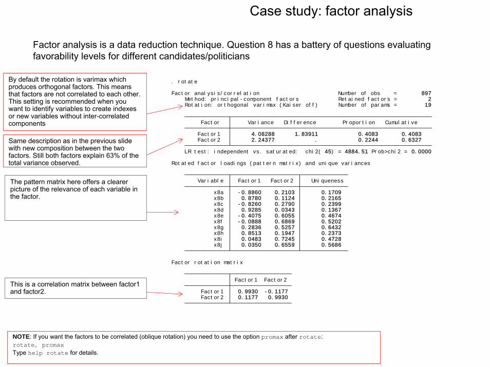
. rotateBy default the rotation is varimax which produces orthogonal factors. This means that factors are not correlated to each other. This setting is recommended when you want to identify variables to create indexes or new variables without inter-correlated components

Same description as in the previous slide with new composition between the two factors. Still both factors explain 63% of the total variance observed.

The pattern matrix here offers a clearer picture of the relevance of each variable in the factor.

This is a correlation matrix between factor1 and factor2.

NOTE: If you want the factors to be correlated (oblique rotation) you need to use the option promax after rotate:rotate, promaxType help rotate for details.

x8j 0.02453 0.29473 x8i 0.02947 0.32580 x8h 0.21436 0.10790 x8g 0.08259 0.24245 x8f -0.00521 0.30564 x8e -0.08565 0.26140 x8d 0.22947 0.03792 x8c -0.19662 0.10498 x8b 0.21892 0.07169 x8a -0.21306 0.07271 Variable Factor1 Factor2

Scoring coefficients (method = regression; based on varimax rotated factors)

(regression scoring assumed). predict x8f1 x8f2

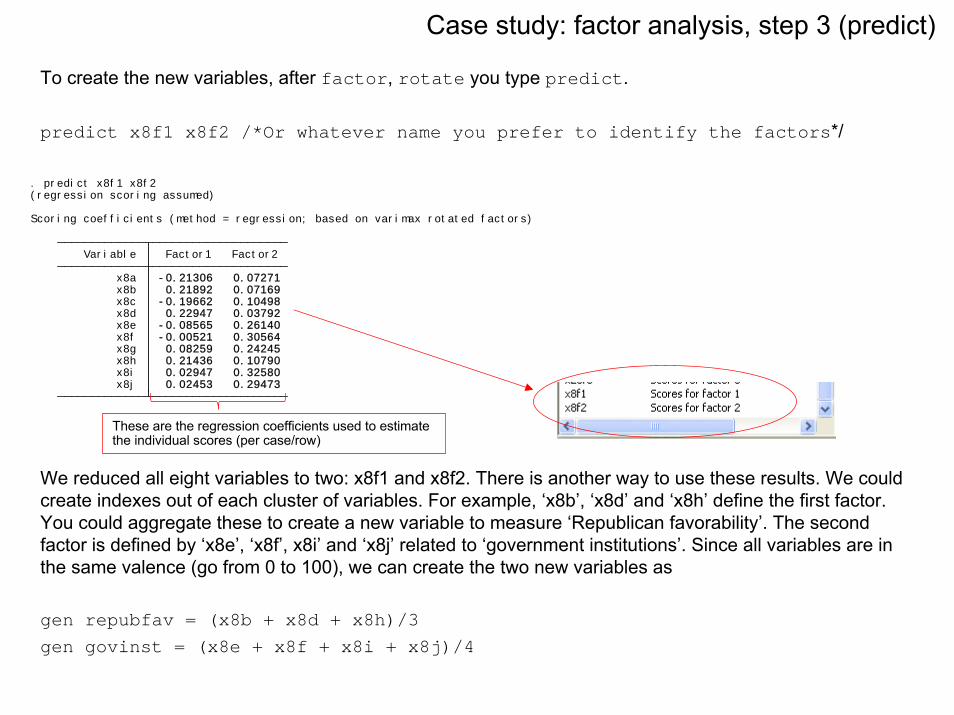
To create the new variables, after factor, rotate you type predict.

predict x8f1 x8f2 /*Or whatever name you prefer to identify the factors*/

Case study: factor analysis, step 3 (predict)

We reduced all eight variables to two: x8f1 and x8f2. There is another way to use these results. We could create indexes out of each cluster of variables. For example, ‘x8b’, ‘x8d’ and ‘x8h’ define the first factor. You could aggregate these to create a new variable to measure ‘Republican favorability’. The second factor is defined by ‘x8e’, ‘x8f’, x8i’ and ‘x8j’ related to ‘government institutions’. Since all variables are in the same valence (go from 0 to 100), we can create the two new variables as

gen repubfav = (x8b + x8d + x8h)/3gen govinst = (x8e + x8f + x8i + x8j)/4

These are the regression coefficients used to estimate the individual scores (per case/row)

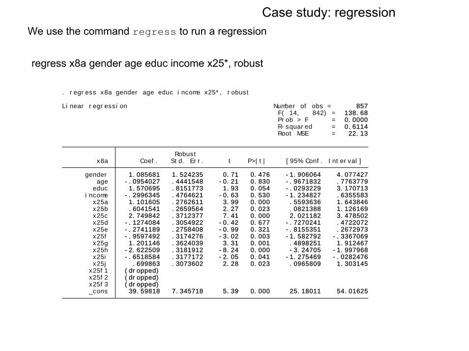
Case study: regressionWe use the command regress to run a regression

regress x8a gender age educ income x25*, robust

_cons 39.59818 7.345718 5.39 0.000 25.18011 54.01625 x25f3 (dropped) x25f2 (dropped) x25f1 (dropped) x25j .699863 .3073602 2.28 0.023 .0965809 1.303145 x25i -.6518584 .3177172 -2.05 0.041 -1.275469 -.0282476 x25h -2.622509 .3181912 -8.24 0.000 -3.24705 -1.997968 x25g 1.201146 .3624039 3.31 0.001 .4898251 1.912467 x25f -.9597492 .3174276 -3.02 0.003 -1.582792 -.3367069 x25e -.2741189 .2758408 -0.99 0.321 -.8155351 .2672973 x25d -.1274084 .3054922 -0.42 0.677 -.7270241 .4722072 x25c 2.749842 .3712377 7.41 0.000 2.021182 3.478502 x25b .6041541 .2659564 2.27 0.023 .0821388 1.126169 x25a 1.101605 .2762611 3.99 0.000 .5593636 1.643846 income -.2996345 .4764621 -0.63 0.530 -1.234827 .6355583 educ 1.570695 .8151773 1.93 0.054 -.0293229 3.170713 age -.0954027 .4441548 -0.21 0.830 -.9671832 .7763779 gender 1.085681 1.524235 0.71 0.476 -1.906064 4.077427 x8a Coef. Std. Err. t P>|t| [95% Conf. Interval] Robust

Root MSE = 22.13 R-squared = 0.6114 Prob > F = 0.0000 F( 14, 842) = 138.68Linear regression Number of obs = 857

. regress x8a gender age educ income x25*, robust

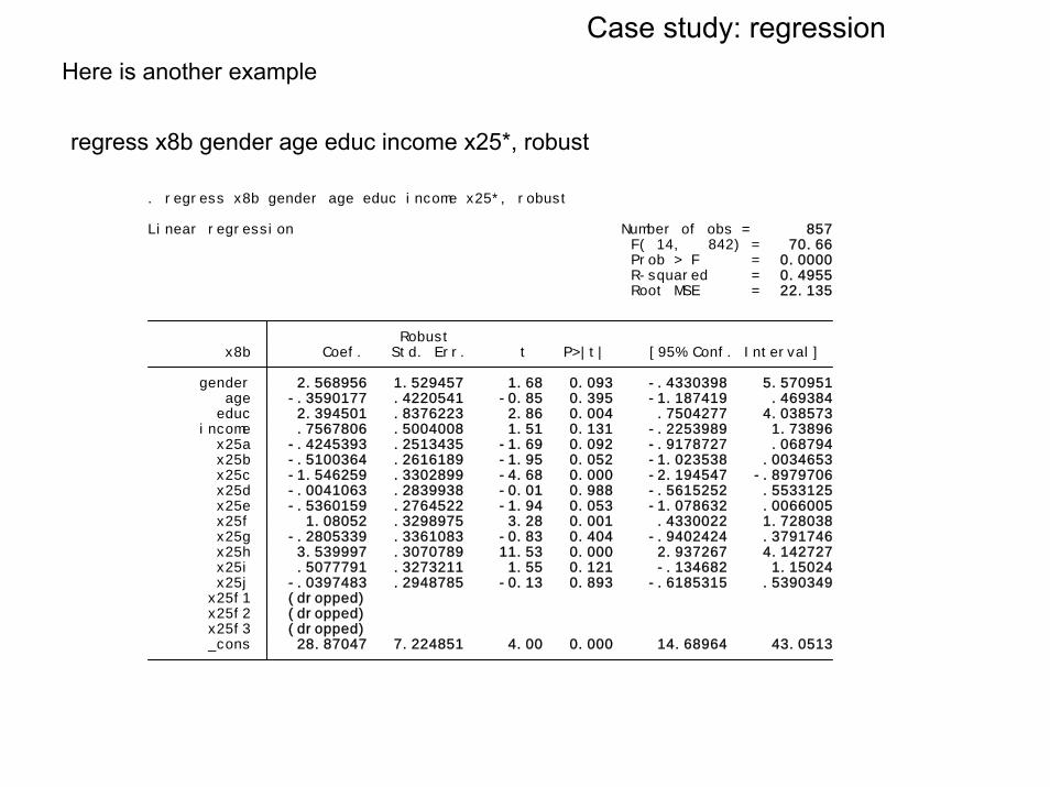
Case study: regressionHere is another example

regress x8b gender age educ income x25*, robust

_cons 28.87047 7.224851 4.00 0.000 14.68964 43.0513 x25f3 (dropped) x25f2 (dropped) x25f1 (dropped) x25j -.0397483 .2948785 -0.13 0.893 -.6185315 .5390349 x25i .5077791 .3273211 1.55 0.121 -.134682 1.15024 x25h 3.539997 .3070789 11.53 0.000 2.937267 4.142727 x25g -.2805339 .3361083 -0.83 0.404 -.9402424 .3791746 x25f 1.08052 .3298975 3.28 0.001 .4330022 1.728038 x25e -.5360159 .2764522 -1.94 0.053 -1.078632 .0066005 x25d -.0041063 .2839938 -0.01 0.988 -.5615252 .5533125 x25c -1.546259 .3302899 -4.68 0.000 -2.194547 -.8979706 x25b -.5100364 .2616189 -1.95 0.052 -1.023538 .0034653 x25a -.4245393 .2513435 -1.69 0.092 -.9178727 .068794 income .7567806 .5004008 1.51 0.131 -.2253989 1.73896 educ 2.394501 .8376223 2.86 0.004 .7504277 4.038573 age -.3590177 .4220541 -0.85 0.395 -1.187419 .469384 gender 2.568956 1.529457 1.68 0.093 -.4330398 5.570951 x8b Coef. Std. Err. t P>|t| [95% Conf. Interval] Robust

Root MSE = 22.135 R-squared = 0.4955 Prob > F = 0.0000 F( 14, 842) = 70.66Linear regression Number of obs = 857

. regress x8b gender age educ income x25*, robust

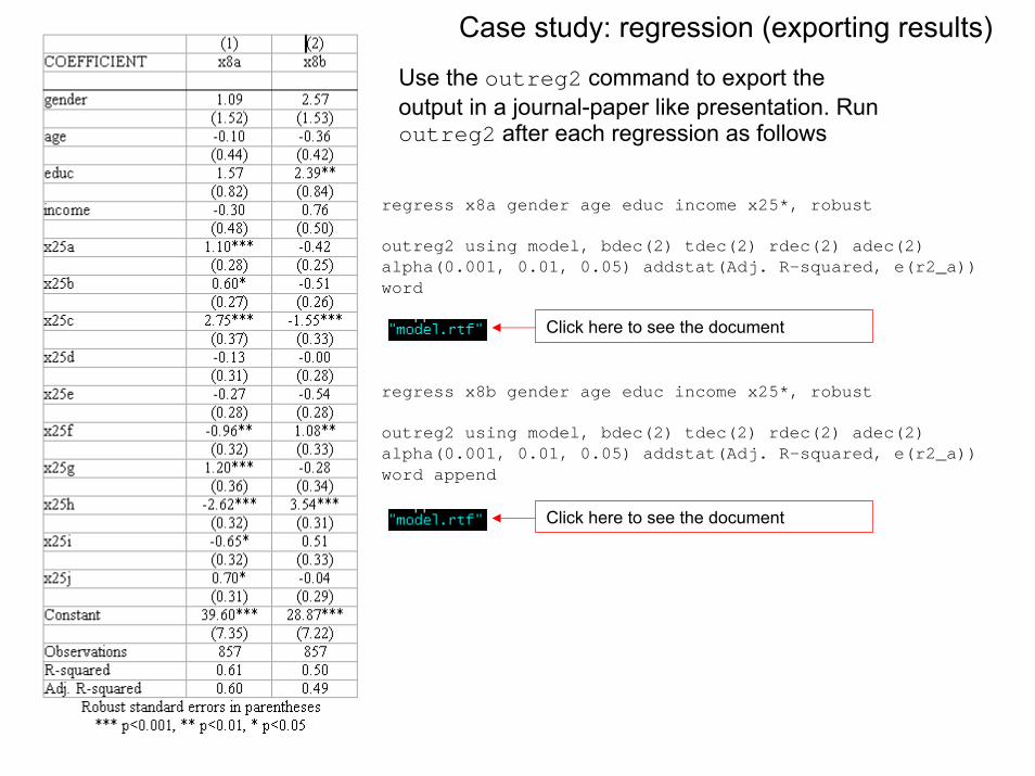
regress x8a gender age educ income x25*, robust

outreg2 using model, bdec(2) tdec(2) rdec(2) adec(2) alpha(0.001, 0.01, 0.05) addstat(Adj. R-squared, e(r2_a)) word

regress x8b gender age educ income x25*, robust

outreg2 using model, bdec(2) tdec(2) rdec(2) adec(2) alpha(0.001, 0.01, 0.05) addstat(Adj. R-squared, e(r2_a)) word append

Case study: regression (exporting results)

Use the outreg2 command to export the output in a journal-paper like presentation. Run outreg2 after each regression as follows

Click here to see the document

Click here to see the document

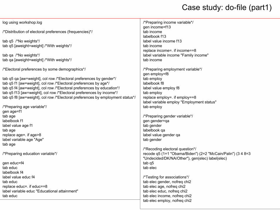
log using workshop.log

/*Distribution of electoral preferences (frequencies)*/

tab q5 /*No weights*/tab q5 [aweight=weight] /*With weights*/

tab qa /*No weights*/tab qa [aweight=weight] /*With weights*/

/*Electoral preferences by some demographics*/

tab q5 qa [aw=weight], col row /*Electoral preferences by gender*/tab q5 f1 [aw=weight], col row /*Electoral preferences by age*/tab q5 f4 [aw=weight], col row /*Electoral preferences by education*/tab q5 f13 [aw=weight], col row /*Electoral preferences by income*/tab q5 f8 [aw=weight], col row /*Electoral preferences by employment status*/

/*Preparing age variable*/gen age=f1tab agelabelbook f1label value age f1tab agereplace age=. if age>8label variable age "Age"tab age

/*Preparing education variable*/

gen educ=f4tab educlabelbook f4label value educ f4tab educreplace educ=. if educ==8label variable educ "Educational attainment"tab educ

/*Preparing income variable*/gen income=f13tab incomelabelbook f13label value income f13tab incomereplace income=. if income==8label variable income "Family income"tab income

/*Preparing employment variable*/gen employ=f8tab employlabelbook f8label value employ f8tab employreplace employ=. if employ==8label variable employ "Employment status"tab employ

/*Preparing gender variable*/gen gender=qatab genderlabelbook qalabel value gender qatab gender

/*Recoding electoral question*/recode q5 (1=1 "Obama/Biden") (2=2 "McCain/Palin") (3 4 8=3 "Undecided/DK/NA/Other"), gen(elec) label(elec)tab q5tab elec

/*Testing for associations*/tab elec gender, nofreq chi2tab elec age, nofreq chi2tab elec educ, nofreq chi2tab elec income, nofreq chi2tab elec employ, nofreq chi2

Case study: do-file (part1)

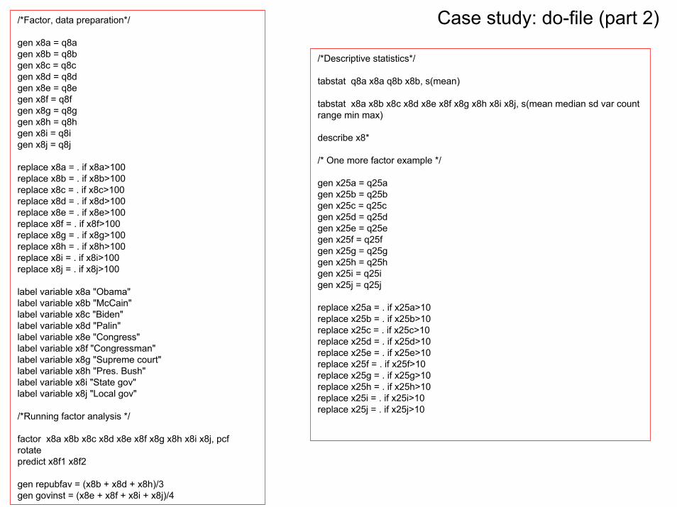
Case study: do-file (part 2)/*Factor, data preparation*/

gen x8a = q8agen x8b = q8bgen x8c = q8cgen x8d = q8dgen x8e = q8egen x8f = q8fgen x8g = q8ggen x8h = q8hgen x8i = q8igen x8j = q8j

replace x8a = . if x8a>100replace x8b = . if x8b>100replace x8c = . if x8c>100replace x8d = . if x8d>100replace x8e = . if x8e>100replace x8f = . if x8f>100replace x8g = . if x8g>100replace x8h = . if x8h>100replace x8i = . if x8i>100replace x8j = . if x8j>100

label variable x8a "Obama"label variable x8b "McCain"label variable x8c "Biden"label variable x8d "Palin"label variable x8e "Congress"label variable x8f "Congressman"label variable x8g "Supreme court"label variable x8h "Pres. Bush"label variable x8i "State gov"label variable x8j "Local gov"

/*Running factor analysis */

factor x8a x8b x8c x8d x8e x8f x8g x8h x8i x8j, pcfrotatepredict x8f1 x8f2

gen repubfav = (x8b + x8d + x8h)/3gen govinst = (x8e + x8f + x8i + x8j)/4

/*Descriptive statistics*/

tabstat q8a x8a q8b x8b, s(mean)

tabstat x8a x8b x8c x8d x8e x8f x8g x8h x8i x8j, s(mean median sd var count range min max)

describe x8*

/* One more factor example */

gen x25a = q25agen x25b = q25bgen x25c = q25cgen x25d = q25dgen x25e = q25egen x25f = q25fgen x25g = q25ggen x25h = q25hgen x25i = q25igen x25j = q25j

replace x25a = . if x25a>10replace x25b = . if x25b>10replace x25c = . if x25c>10replace x25d = . if x25d>10replace x25e = . if x25e>10replace x25f = . if x25f>10replace x25g = . if x25g>10replace x25h = . if x25h>10replace x25i = . if x25i>10replace x25j = . if x25j>10

Case study: do-file (part 3)

label variable x25a "A woman should be able to get an abortion if she wants one in the first three months of pregnancy, no matter what the reason"label variable x25b "Gay couples should be allowed to marry, giving them full legal rights of married couples"label variable x25c "The government should provide health care coverage to all citizens who can’t afford it, even if it means higher taxes"label variable x25d "Government regulation of financial institutions should be greatly increased"label variable x25e "The government should have let financial institutions that got into trouble over bad mortgage debt go out of business rather than trying to rescue them"label variable x25f "The government should allow offshore drilling for oil and gas in the waters off the U.S. coast "label variable x25g "Congress should pass stricter laws to protect the environment and reduce global warming, even if the economic costs are high"label variable x25h "Our troops should stay in Iraq without a timetable for withdrawal until the Iraqi government is stable"label variable x25i "Government should cut taxes on businesses to help the economy"label variable x25j "The government should help people who can’t afford their mortgage payments by suspending foreclosures until the economy has improved"

factor x25a x25b x25c x25d x25e x25f x25g x25h x25i x25j, pcfrotatepredict x25f1 x25f2 x25f3

/*Regression*/

regress x8a gender age educ income x25*, robustregress x8b gender age educ income x25*, robust

Exploring data: annotated output

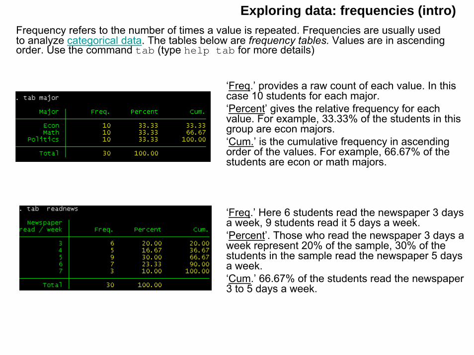
Exploring data: frequencies (intro)Frequency refers to the number of times a value is repeated. Frequencies are usually used to analyze categorical data. The tables below are frequency tables. Values are in ascending order. Use the command tab (type help tab for more details)

‘Freq.’ provides a raw count of each value. In this case 10 students for each major.‘Percent’ gives the relative frequency for each value. For example, 33.33% of the students in this group are econ majors.‘Cum.’ is the cumulative frequency in ascending order of the values. For example, 66.67% of the students are econ or math majors.

‘Freq.’ Here 6 students read the newspaper 3 days a week, 9 students read it 5 days a week.‘Percent’. Those who read the newspaper 3 days a week represent 20% of the sample, 30% of the students in the sample read the newspaper 5 days a week.‘Cum.’ 66.67% of the students read the newspaper 3 to 5 days a week.

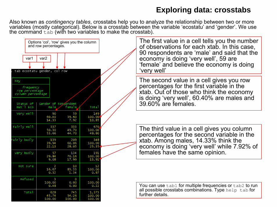
Exploring data: crosstabsAlso known as contingency tables, crosstabs help you to analyze the relationship between two or more variables (mostly categorical). Below is a crosstab between the variable ‘ecostatu’ and ‘gender’. We use the command tab (with two variables to make the crosstab).

The first value in a cell tells you the number of observations for each xtab. In this case, 90 respondents are ‘male’ and said that the economy is doing ‘very well’, 59 are ‘female’ and believe the economy is doing ‘very well’The second value in a cell gives you row percentages for the first variable in the xtab. Out of those who think the economy is doing ‘very well’, 60.40% are males and 39.60% are females.

The third value in a cell gives you column percentages for the second variable in the xtab. Among males, 14.33% think the economy is doing ‘very well’ while 7.92% of females have the same opinion.

var1 var2

Options ‘col’, ‘row’ gives you the column and row percentages.

You can use tab1 for multiple frequencies or tab2 to run all possible crosstabs combinations. Type help tab for further details.

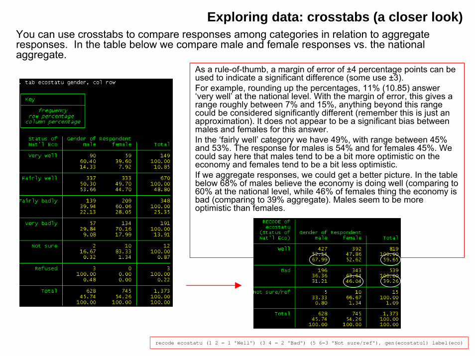
Exploring data: crosstabs (a closer look)You can use crosstabs to compare responses among categories in relation to aggregate responses. In the table below we compare male and female responses vs. the national aggregate.

As a rule-of-thumb, a margin of error of ±4 percentage points can be used to indicate a significant difference (some use ±3). For example, rounding up the percentages, 11% (10.85) answer ‘very well’ at the national level. With the margin of error, this gives a range roughly between 7% and 15%, anything beyond this range could be considered significantly different (remember this is just an approximation). It does not appear to be a significant bias between males and females for this answer.In the ‘fairly well’ category we have 49%, with range between 45% and 53%. The response for males is 54% and for females 45%. We could say here that males tend to be a bit more optimistic on the economy and females tend to be a bit less optimistic. If we aggregate responses, we could get a better picture. In the table below 68% of males believe the economy is doing well (comparing to 60% at the national level, while 46% of females thing the economy is bad (comparing to 39% aggregate). Males seem to be more optimistic than females.

recode ecostatu (1 2 = 1 "Well") (3 4 = 2 "Bad") (5 6=3 "Not sure/ref"), gen(ecostatu1) label(eco)

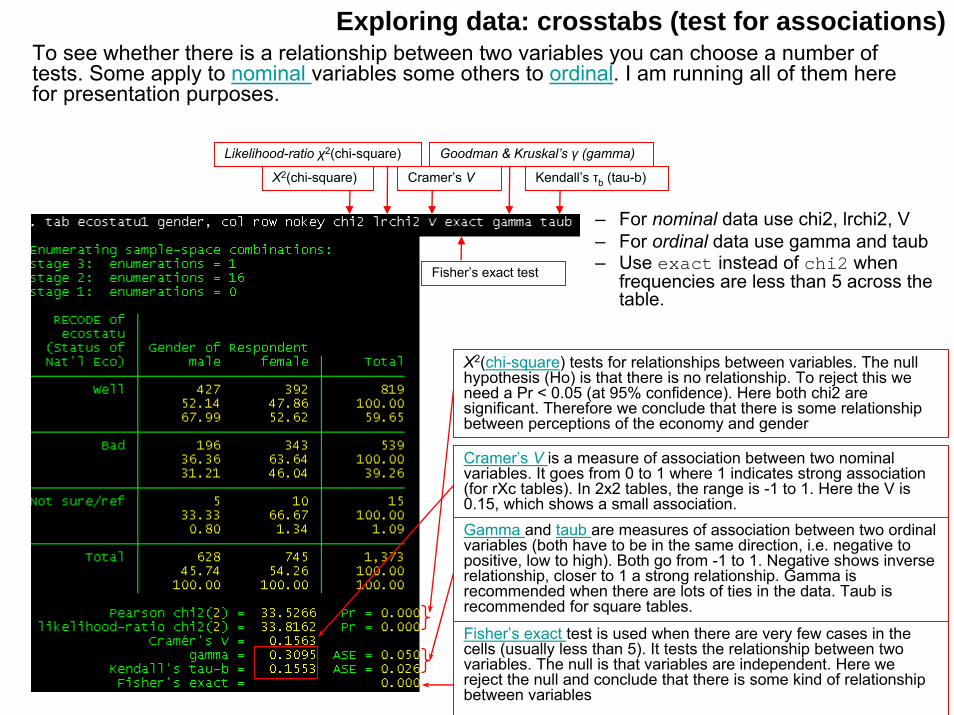
Exploring data: crosstabs (test for associations)To see whether there is a relationship between two variables you can choose a number of tests. Some apply to nominal variables some others to ordinal. I am running all of them here for presentation purposes.

– For nominal data use chi2, lrchi2, V– For ordinal data use gamma and taub– Use exact instead of chi2 when

frequencies are less than 5 across the table.

X2(chi-square)

Likelihood-ratio χ2(chi-square)

Cramer’s V

Fisher’s exact test

Goodman & Kruskal’s γ (gamma)

Kendall’s τb (tau-b)

X2(chi-square) tests for relationships between variables. The null hypothesis (Ho) is that there is no relationship. To reject this we need a Pr < 0.05 (at 95% confidence). Here both chi2 are significant. Therefore we conclude that there is some relationship between perceptions of the economy and gender

Cramer’s V is a measure of association between two nominal variables. It goes from 0 to 1 where 1 indicates strong association (for rXc tables). In 2x2 tables, the range is -1 to 1. Here the V is 0.15, which shows a small association.Gamma and taub are measures of association between two ordinal variables (both have to be in the same direction, i.e. negative to positive, low to high). Both go from -1 to 1. Negative shows inverse relationship, closer to 1 a strong relationship. Gamma is recommended when there are lots of ties in the data. Taub is recommended for square tables.

Fisher’s exact test is used when there are very few cases in the cells (usually less than 5). It tests the relationship between two variables. The null is that variables are independent. Here we reject the null and conclude that there is some kind of relationship between variables

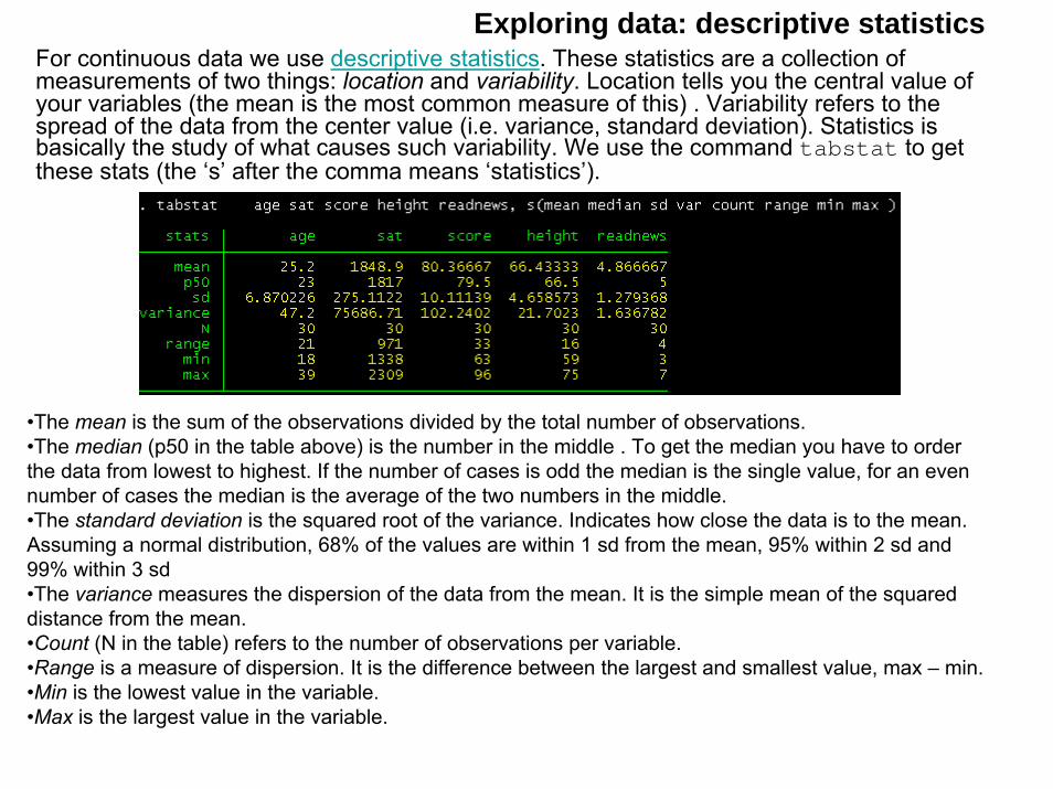
Exploring data: descriptive statisticsFor continuous data we use descriptive statistics. These statistics are a collection of measurements of two things: location and variability. Location tells you the central value of your variables (the mean is the most common measure of this) . Variability refers to the spread of the data from the center value (i.e. variance, standard deviation). Statistics is basically the study of what causes such variability. We use the command tabstat to get these stats (the ‘s’ after the comma means ‘statistics’).

•The mean is the sum of the observations divided by the total number of observations. •The median (p50 in the table above) is the number in the middle . To get the median you have to order the data from lowest to highest. If the number of cases is odd the median is the single value, for an even number of cases the median is the average of the two numbers in the middle.•The standard deviation is the squared root of the variance. Indicates how close the data is to the mean. Assuming a normal distribution, 68% of the values are within 1 sd from the mean, 95% within 2 sd and 99% within 3 sd•The variance measures the dispersion of the data from the mean. It is the simple mean of the squared distance from the mean.•Count (N in the table) refers to the number of observations per variable.•Range is a measure of dispersion. It is the difference between the largest and smallest value, max – min.•Min is the lowest value in the variable.•Max is the largest value in the variable.

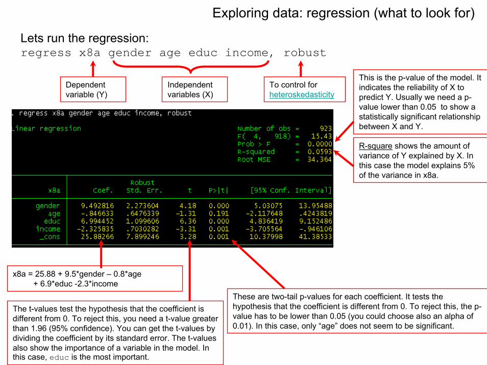
Exploring data: regression (what to look for)

This is the p-value of the model. It indicates the reliability of X to predict Y. Usually we need a p-value lower than 0.05 to show a statistically significant relationship between X and Y.

R-square shows the amount of variance of Y explained by X. In this case the model explains 5% of the variance in x8a.

Lets run the regression:regress x8a gender age educ income, robust

These are two-tail p-values for each coefficient. It tests the hypothesis that the coefficient is different from 0. To reject this, the p-value has to be lower than 0.05 (you could choose also an alpha of 0.01). In this case, only “age” does not seem to be significant.

The t-values test the hypothesis that the coefficient is different from 0. To reject this, you need a t-value greater than 1.96 (95% confidence). You can get the t-values by dividing the coefficient by its standard error. The t-values also show the importance of a variable in the model. In this case, educ is the most important.

x8a = 25.88 + 9.5*gender – 0.8*age + 6.9*educ -2.3*income

Dependent variable (Y)

Independent variables (X)

To control for heteroskedasticity

Once you define your final model, you can export your regression results using either your log file or the option outreg2. For the log you just open it using any word processor and copy-and-paste the regression table into excel or word. The command outreg2 gives you the type of presentation you see in scholar’s papers. Let’s say the final regression is regress csat percent percent2 highAfter running the regression type the following if you want to export the results to excel*outreg2 using results, bdec(2) tdec(2) rdec(2) adec(2) alpha(0.001, 0.01, 0.05) addstat(Adj. R-squared, e(r2_a)) excelOr this if you want to export to wordoutreg2 using results, bdec(2) tdec(2) rdec(2) adec(2) alpha(0.001, 0.01, 0.05) addstat(Adj. R-squared, e(r2_a)) wordYou will see this in Stata’s output window

Exploring data: regression, publishing regression output (outreg2)

For excel

For word Click here to see the output, a excel/word window will open

Name of the file for the output

Set # of decimals for coefficients

Set # of decimals for auxiliary statistics

Set # of decimals for the R2

Set # of decimals for added statistics (addstat option)

Click on seeoutto browse the results

Levels of significance

Include some additional statistic, in this case adj. R-sqr. You can select any statistics on the return lists (e-class, r-class or s-class). After running the regression type ereturn list for a list of available statistics.

Type help outreg2 for more details. If you do not see outreg2, you may have to install it by typing ssc install outreg2. If this does not work type findit outreg2, select from the list and click “install”.

Note: If you get the following error message (when you use the option append or replace it means that you need to close the excel/word window.

*See the following document for some additional info/tips http://www.fiu.edu/~tardanic/brianne.pdf

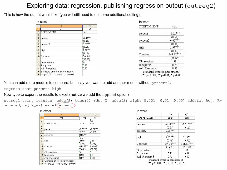
This is how the output would like (you will still need to do some additional editing):

Exploring data: regression, publishing regression output (outreg2)

In excel In word

You can add more models to compare. Lets say you want to add another model without percent2:regress csat percent high

Now type to export the results to excel (notice we add the append option)outreg2 using results, bdec(2) tdec(2) rdec(2) adec(2) alpha(0.001, 0.01, 0.05) addstat(Adj. R-squared, e(r2_a)) excel append

In excel In word