Embed Size (px)
Citation preview

Ansoft High Frequency Structure Simulator
Getting Started: A Dielectric Resonator Antenna Problem
�
This Getting Started guide is for the Beta release of HFSS 9.0. A different guide will accompany the Final �release.
February 2003

NoticeThe information contained in this document is subject to change without notice.Ansoft makes no warranty of any kind with regard to this material, including, but not limited to, the implied warranties of merchantability and fitness for a particular purpose. Ansoft shall not be liable for errors contained herein or for incidental or consequential damages in connection with the fur-nishing, performance, or use of this material.This document contains proprietary information which is protected by copyright. All rights are reserved.
Ansoft Corporation�Four Station Square�Suite 200�Pittsburgh, PA 15219�(412) 261 - 3200
Microsoft® Windows® is a registered trademark of Microsoft Corporation.UNIX® is a registered trademark of UNIX Systems Laboratories, Inc.
© Copyright 2003 Ansoft Corporation
ii
Printing HistoryNew editions of this manual will incorporate all material updated since the previous edition. The manual printing date, which indicates the manual’s current edition, changes when a new edition is printed. Minor corrections and updates which are incorporated at reprint do not cause the date to change.Update packages may be issued between editions and contain additional and/or replacement pages to be merged into the manual by the user. Note that pages which are rearranged due to changes on a previous page are not considered to be revised.
Edition Date Software Revision
1.0 February 2003 9.0
iii
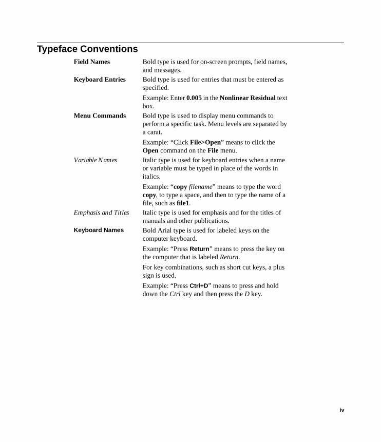
Typeface ConventionsField Names Bold type is used for on-screen prompts, field names,
and messages.Keyboard Entries Bold type is used for entries that must be entered as
specified. Example: Enter 0.005 in the Nonlinear Residual text box.
Menu Commands Bold type is used to display menu commands to perform a specific task. Menu levels are separated by a carat.Example: “Click File>Open” means to click the Open command on the File menu.
Variable Names Italic type is used for keyboard entries when a name or variable must be typed in place of the words in italics. Example: “copy filename” means to type the word copy, to type a space, and then to type the name of a file, such as file1.
Emphasis and Titles Italic type is used for emphasis and for the titles of manuals and other publications.
Keyboard Names Bold Arial type is used for labeled keys on the computer keyboard.Example: “Press Return” means to press the key on the computer that is labeled Return.For key combinations, such as short cut keys, a plus sign is used. Example: “Press Ctrl+D” means to press and hold down the Ctrl key and then press the D key.
iv

Table of Contents
1. Introduction . . . . . . . . . . . . . . . . . . . . . . . . . . . . . . . . . . . . . . . . . . . . . . . 1-1The Sample Problem . . . . . . . . . . . . . . . . . . . . . . . . . . . . . . . . . . . . . . . . . . . . . . . . . . . . . 1-2Results for Analysis . . . . . . . . . . . . . . . . . . . . . . . . . . . . . . . . . . . . . . . . . . . . . . . . . . . . . 1-3
2. Creating the New Project . . . . . . . . . . . . . . . . . . . . . . . . . . . . . . . . . . . . 2-1Overview of the Interface . . . . . . . . . . . . . . . . . . . . . . . . . . . . . . . . . . . . . . . . . . . . . . . . . 2-2Create the New Project . . . . . . . . . . . . . . . . . . . . . . . . . . . . . . . . . . . . . . . . . . . . . . . . . . . 2-4
Add the New Project . . . . . . . . . . . . . . . . . . . . . . . . . . . . . . . . . . . . . . . . . . . . . . . . . . 2-4Insert an HFSS Design . . . . . . . . . . . . . . . . . . . . . . . . . . . . . . . . . . . . . . . . . . . . . . . . 2-4Add Project Notes . . . . . . . . . . . . . . . . . . . . . . . . . . . . . . . . . . . . . . . . . . . . . . . . . . . . 2-5Save the Project . . . . . . . . . . . . . . . . . . . . . . . . . . . . . . . . . . . . . . . . . . . . . . . . . . . . . 2-5
3. Creating the Model . . . . . . . . . . . . . . . . . . . . . . . . . . . . . . . . . . . . . . . . . 3-1Select the Solution Type . . . . . . . . . . . . . . . . . . . . . . . . . . . . . . . . . . . . . . . . . . . . . . . . . . 3-2Set Up the Drawing Region . . . . . . . . . . . . . . . . . . . . . . . . . . . . . . . . . . . . . . . . . . . . . . . 3-3
Overview of the 3D Modeler Window . . . . . . . . . . . . . . . . . . . . . . . . . . . . . . . . . . . . 3-3Coordinate System Settings . . . . . . . . . . . . . . . . . . . . . . . . . . . . . . . . . . . . . . . . . . . . 3-4Units Settings . . . . . . . . . . . . . . . . . . . . . . . . . . . . . . . . . . . . . . . . . . . . . . . . . . . . . . . 3-4Grid Settings . . . . . . . . . . . . . . . . . . . . . . . . . . . . . . . . . . . . . . . . . . . . . . . . . . . . . . . . 3-4
Create the Geometry . . . . . . . . . . . . . . . . . . . . . . . . . . . . . . . . . . . . . . . . . . . . . . . . . . . . . 3-5Draw the Cavity . . . . . . . . . . . . . . . . . . . . . . . . . . . . . . . . . . . . . . . . . . . . . . . . . . . . . 3-5
Draw the Sphere . . . . . . . . . . . . . . . . . . . . . . . . . . . . . . . . . . . . . . . . . . . . . . . . . . . . . . . . . 3-5Rename the Sphere . . . . . . . . . . . . . . . . . . . . . . . . . . . . . . . . . . . . . . . . . . . . . . . . . . . . . . . 3-6Split the Cavity . . . . . . . . . . . . . . . . . . . . . . . . . . . . . . . . . . . . . . . . . . . . . . . . . . . . . . . . . . 3-6Modify the Cavity’s Attributes. . . . . . . . . . . . . . . . . . . . . . . . . . . . . . . . . . . . . . . . . . . . . . 3-7
Assign a Color to the Cavity . . . . . . . . . . . . . . . . . . . . . . . . . . . . . . . . . . . . . . . . . . . . 3-7
Contents-1

Getting Started: A Dielectric Resonator Antenna Problem
Assign a Transparency to the Cavity. . . . . . . . . . . . . . . . . . . . . . . . . . . . . . . . . . . . . . 3-8Verify Lighting Attributes are Disabled . . . . . . . . . . . . . . . . . . . . . . . . . . . . . . . . . . . 3-8Verify the Cavity’s Material . . . . . . . . . . . . . . . . . . . . . . . . . . . . . . . . . . . . . . . . . . . . 3-8
Draw the DRA . . . . . . . . . . . . . . . . . . . . . . . . . . . . . . . . . . . . . . . . . . . . . . . . . . . . . . 3-9Draw the Sphere . . . . . . . . . . . . . . . . . . . . . . . . . . . . . . . . . . . . . . . . . . . . . . . . . . . . . . . . . 3-9Rename the Sphere . . . . . . . . . . . . . . . . . . . . . . . . . . . . . . . . . . . . . . . . . . . . . . . . . . . . . . . 3-10Split the DRA . . . . . . . . . . . . . . . . . . . . . . . . . . . . . . . . . . . . . . . . . . . . . . . . . . . . . . . . . . . 3-10Modify DRA’s Attributes. . . . . . . . . . . . . . . . . . . . . . . . . . . . . . . . . . . . . . . . . . . . . . . . . . 3-11
Assign a Color to the DRA . . . . . . . . . . . . . . . . . . . . . . . . . . . . . . . . . . . . . . . . . . . . . 3-11Assign a Transparency to the DRA. . . . . . . . . . . . . . . . . . . . . . . . . . . . . . . . . . . . . . . 3-11Create and Assign a New Material to the DRA . . . . . . . . . . . . . . . . . . . . . . . . . . . . . 3-12
Create the Annular Feed Ring . . . . . . . . . . . . . . . . . . . . . . . . . . . . . . . . . . . . . . . . . . 3-14Draw Circle1 . . . . . . . . . . . . . . . . . . . . . . . . . . . . . . . . . . . . . . . . . . . . . . . . . . . . . . . . . . . 3-14Draw Circle2 . . . . . . . . . . . . . . . . . . . . . . . . . . . . . . . . . . . . . . . . . . . . . . . . . . . . . . . . . . . 3-15Subtract Circle1 from Circle2 . . . . . . . . . . . . . . . . . . . . . . . . . . . . . . . . . . . . . . . . . . . . . . 3-15Rename Circle2 . . . . . . . . . . . . . . . . . . . . . . . . . . . . . . . . . . . . . . . . . . . . . . . . . . . . . . . . . 3-17Modify the Annular Feed Ring’s Attributes. . . . . . . . . . . . . . . . . . . . . . . . . . . . . . . . . . . . 3-17
Assign a Color to the Annular Feed Ring . . . . . . . . . . . . . . . . . . . . . . . . . . . . . . . . . . 3-17Verify Annular Feed Ring’s Transparency . . . . . . . . . . . . . . . . . . . . . . . . . . . . . . . . . 3-17
Draw the Feed Gap . . . . . . . . . . . . . . . . . . . . . . . . . . . . . . . . . . . . . . . . . . . . . . . . . . . 3-18Draw the Rectangle . . . . . . . . . . . . . . . . . . . . . . . . . . . . . . . . . . . . . . . . . . . . . . . . . . . . . . 3-18Intersect the Rectangle and the Annular Feed Ring . . . . . . . . . . . . . . . . . . . . . . . . . . . . . . 3-19
Rename the Rectangle . . . . . . . . . . . . . . . . . . . . . . . . . . . . . . . . . . . . . . . . . . . . . . . . . 3-20Modify the Feed Gap’s Attributes . . . . . . . . . . . . . . . . . . . . . . . . . . . . . . . . . . . . . . . . . . . 3-20
Assign a Color to the Feed Gap . . . . . . . . . . . . . . . . . . . . . . . . . . . . . . . . . . . . . . . . . 3-20Assign a Transparency to the Feed Gap . . . . . . . . . . . . . . . . . . . . . . . . . . . . . . . . . . . 3-20
Draw the Air Volume . . . . . . . . . . . . . . . . . . . . . . . . . . . . . . . . . . . . . . . . . . . . . . . . . 3-21Draw the Polyhedron . . . . . . . . . . . . . . . . . . . . . . . . . . . . . . . . . . . . . . . . . . . . . . . . . . . . . 3-21Rename the Polyhedron . . . . . . . . . . . . . . . . . . . . . . . . . . . . . . . . . . . . . . . . . . . . . . . . . . . 3-22Modify the Air Volume’s Attributes . . . . . . . . . . . . . . . . . . . . . . . . . . . . . . . . . . . . . . . . . 3-22
Assign a Color to the Air Volume. . . . . . . . . . . . . . . . . . . . . . . . . . . . . . . . . . . . . . . . 3-22Assign a Transparency to the Air Volume . . . . . . . . . . . . . . . . . . . . . . . . . . . . . . . . . 3-22Verify Air Volume’s Material. . . . . . . . . . . . . . . . . . . . . . . . . . . . . . . . . . . . . . . . . . . 3-22
Split the Model for Symmetry . . . . . . . . . . . . . . . . . . . . . . . . . . . . . . . . . . . . . . . . . . 3-23
4. Setting Up the Problem . . . . . . . . . . . . . . . . . . . . . . . . . . . . . . . . . . . . . . 4-1Set Up Boundaries and Excitations . . . . . . . . . . . . . . . . . . . . . . . . . . . . . . . . . . . . . . . . . 4-2
Boundary Conditions . . . . . . . . . . . . . . . . . . . . . . . . . . . . . . . . . . . . . . . . . . . . . . . . . 4-2Excitation Conditions . . . . . . . . . . . . . . . . . . . . . . . . . . . . . . . . . . . . . . . . . . . . . . . . . 4-2Assigning Boundaries . . . . . . . . . . . . . . . . . . . . . . . . . . . . . . . . . . . . . . . . . . . . . . . . . 4-3
Assign a Radiation Boundary to the Air Volume. . . . . . . . . . . . . . . . . . . . . . . . . . . . . . . . 4-3Assign a Perfect E Boundary to the Air Volume . . . . . . . . . . . . . . . . . . . . . . . . . . . . . . . . 4-4Assign a Perfect H Boundary to the Annular Feed Ring . . . . . . . . . . . . . . . . . . . . . . . . . . 4-7
Contents-2

Getting Started: A Dielectric Resonator Antenna Problem
Assign a Symmetry Boundary to the Model . . . . . . . . . . . . . . . . . . . . . . . . . . . . . . . . . . . 4-8Assigning Excitations . . . . . . . . . . . . . . . . . . . . . . . . . . . . . . . . . . . . . . . . . . . . . . . . . 4-10
Assign a Lumped Port Across the Gap. . . . . . . . . . . . . . . . . . . . . . . . . . . . . . . . . . . . . . . . 4-10Modify the Impedance Multiplier . . . . . . . . . . . . . . . . . . . . . . . . . . . . . . . . . . . . . . . . . . . 4-12
Verify All Boundary and Excitation Assignments . . . . . . . . . . . . . . . . . . . . . . . . . . . 4-13
5. Generating A Solution . . . . . . . . . . . . . . . . . . . . . . . . . . . . . . . . . . . . . . . 5-1Specify Solution Options . . . . . . . . . . . . . . . . . . . . . . . . . . . . . . . . . . . . . . . . . . . . . . . . . 5-2
Add a Solution Setup . . . . . . . . . . . . . . . . . . . . . . . . . . . . . . . . . . . . . . . . . . . . . . . . . 5-2Add a Frequency Sweep to the Solution Setup . . . . . . . . . . . . . . . . . . . . . . . . . . . . . . . . . 5-5
Define Mesh Operations . . . . . . . . . . . . . . . . . . . . . . . . . . . . . . . . . . . . . . . . . . . . . . . 5-6Validate the Project Setup . . . . . . . . . . . . . . . . . . . . . . . . . . . . . . . . . . . . . . . . . . . . . . . . . 5-8Generate the Solution . . . . . . . . . . . . . . . . . . . . . . . . . . . . . . . . . . . . . . . . . . . . . . . . . . . . 5-9
View the Solution Data . . . . . . . . . . . . . . . . . . . . . . . . . . . . . . . . . . . . . . . . . . . . . . . . 5-10View the Profile Data . . . . . . . . . . . . . . . . . . . . . . . . . . . . . . . . . . . . . . . . . . . . . . . . . . . . . 5-10View Convergence Data. . . . . . . . . . . . . . . . . . . . . . . . . . . . . . . . . . . . . . . . . . . . . . . . . . . 5-11View Matrix Data . . . . . . . . . . . . . . . . . . . . . . . . . . . . . . . . . . . . . . . . . . . . . . . . . . . . . . . . 5-12
6. Analyzing the Solution . . . . . . . . . . . . . . . . . . . . . . . . . . . . . . . . . . . . . . 6-1Create Modal S-Parameters Reports . . . . . . . . . . . . . . . . . . . . . . . . . . . . . . . . . . . . . . . . . 6-2
Create an S-Parameters Report of S11 . . . . . . . . . . . . . . . . . . . . . . . . . . . . . . . . . . . . 6-2Create an S-Parameters Report of Z11 . . . . . . . . . . . . . . . . . . . . . . . . . . . . . . . . . . . . 6-5
Create Field Overlay Plots . . . . . . . . . . . . . . . . . . . . . . . . . . . . . . . . . . . . . . . . . . . . . . . . 6-8Create a Mag E Field Overlay Plot . . . . . . . . . . . . . . . . . . . . . . . . . . . . . . . . . . . . . . . 6-8
Modify the Mag E Plot’s Attributes . . . . . . . . . . . . . . . . . . . . . . . . . . . . . . . . . . . . . . . . . . 6-10Create a Phase Animation of the Mag E Plot . . . . . . . . . . . . . . . . . . . . . . . . . . . . . . . . . . . 6-12
Contents-3

Getting Started: A Dielectric Resonator Antenna Problem
Contents-4

Introduction
HFSS is an interactive software package for calculating the electromagnetic behavior of a �structure. The software also includes post-processing commands for analyzing the electromagnetic behavior of a structure in more detail. Using HFSS, you can compute:• Basic electromagnetic field quantities and, for open boundary problems, radiated near and far
fields.• Characteristic port impedances and propagation constants.• Generalized S-parameters and S-parameters renormalized to specific port impedances.• The eigenmodes, or resonances, of a structure.You are expected to draw the structure, specify material characteristics for each object, and identify ports, sources, or special surface characteristics. The system then generates the necessary field solutions. HFSS version 9 is currently available on PCs running Windows NT 4.0, 2000 Professional, and XP Professional.
Introduction 1-1
Getting Started: A Dielectric Resonator Antenna Problem
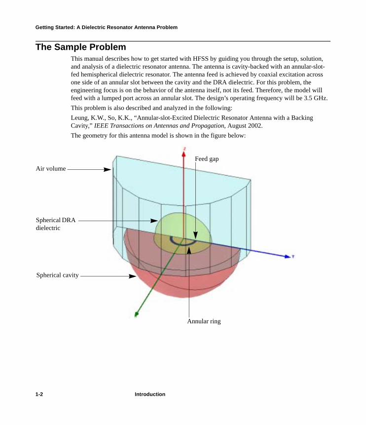
The Sample Problem This manual describes how to get started with HFSS by guiding you through the setup, solution, and analysis of a dielectric resonator antenna. The antenna is cavity-backed with an annular-slot-fed hemispherical dielectric resonator. The antenna feed is achieved by coaxial excitation across one side of an annular slot between the cavity and the DRA dielectric. For this problem, the �engineering focus is on the behavior of the antenna itself, not its feed. Therefore, the model will feed with a lumped port across an annular slot. The design’s operating frequency will be 3.5 GHz. This problem is also described and analyzed in the following:Leung, K.W., So, K.K., “Annular-slot-Excited Dielectric Resonator Antenna with a Backing �Cavity,” IEEE Transactions on Antennas and Propagation, August 2002. The geometry for this antenna model is shown in the figure below:
Air volume
Spherical DRA dielectric
Spherical cavity
Annular ring
Feed gap
1-2 Introduction

Getting Started: A Dielectric Resonator Antenna Problem
Results for AnalysisAfter setting up the antenna problem and generating a solution, you will: • Create Modal S-parameter reports. • Create a field overlay plot of the magnitude of E for the antenna cavity’s face.• Create an animation of the mag-E field overlay plot.
Time It should take you approximately 3 hours to work through this manual.
Introduction 1-3

Getting Started: A Dielectric Resonator Antenna Problem
1-4 Introduction

Creating the New Project
This guide assumes that HFSS has already been installed as described in the Installation Guide.
Your goals in this chapter are as follows:• Create a new project.• Add an HFSS design to the project.
Note If you have not installed the software or you are not yet set up to run the software, STOP! Follow the instructions in the Installation Guide.
Time It should take you approximately 15 minutes to work through this chapter.
Creating the New Project 2-1
Getting Started: A Dielectric Resonator Antenna Problem
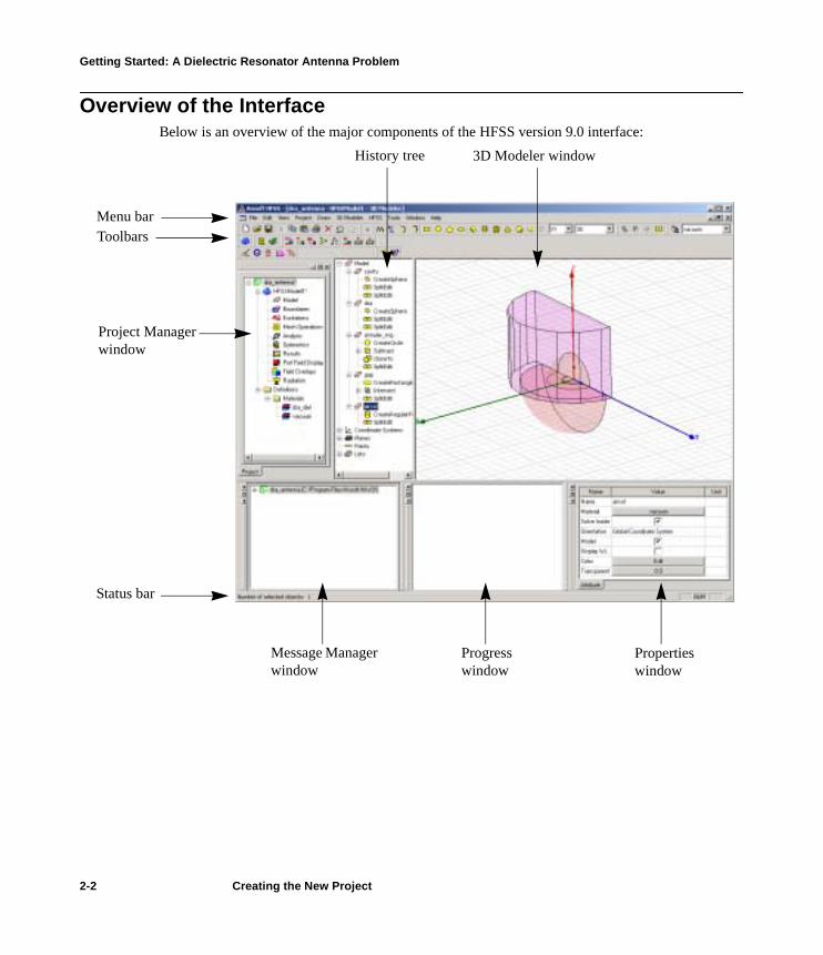
Overview of the InterfaceBelow is an overview of the major components of the HFSS version 9.0 interface:
Menu barToolbars
Status bar
History tree
Project Manager window
Message Manager window
Progress window
Properties window
3D Modeler window
2-2 Creating the New Project
Getting Started: A Dielectric Resonator Antenna Problem
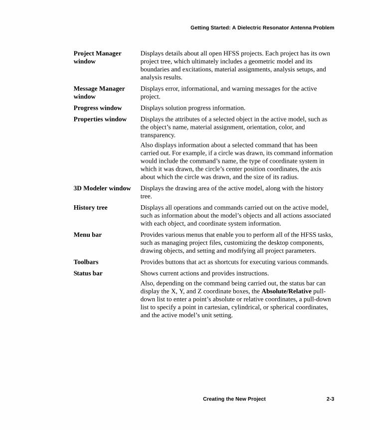
Project Manager window
Displays details about all open HFSS projects. Each project has its own project tree, which ultimately includes a geometric model and its boundaries and excitations, material assignments, analysis setups, and analysis results.
Message Manager window
Displays error, informational, and warning messages for the active project.
Progress window Displays solution progress information.
Properties window Displays the attributes of a selected object in the active model, such as the object’s name, material assignment, orientation, color, and transparency. Also displays information about a selected command that has been carried out. For example, if a circle was drawn, its command information would include the command’s name, the type of coordinate system in which it was drawn, the circle’s center position coordinates, the axis about which the circle was drawn, and the size of its radius.
3D Modeler window Displays the drawing area of the active model, along with the history tree.
History tree Displays all operations and commands carried out on the active model, such as information about the model’s objects and all actions associated with each object, and coordinate system information.
Menu bar Provides various menus that enable you to perform all of the HFSS tasks, such as managing project files, customizing the desktop components, drawing objects, and setting and modifying all project parameters.
Toolbars Provides buttons that act as shortcuts for executing various commands.
Status bar Shows current actions and provides instructions. Also, depending on the command being carried out, the status bar can display the X, Y, and Z coordinate boxes, the Absolute/Relative pull-down list to enter a point’s absolute or relative coordinates, a pull-down list to specify a point in cartesian, cylindrical, or spherical coordinates, and the active model’s unit setting.
Creating the New Project 2-3

Getting Started: A Dielectric Resonator Antenna Problem
Create the New Project The first step in using HFSS to solve a problem, is to create a project in which the data associated with the problem can be saved.
Add the New ProjectTo add a new project HFSS:• Click File>New.A new project is listed in the project tree in the Project Manager window. It is named projectn by default, where n is the order in which the project was added to the current session. Project �definitions, such as boundaries and material assignments, are stored under the project name in the project tree.
Insert an HFSS DesignThe next step for this antenna problem is to insert an HFSS design into the new project. To insert an HFSS design into the project, do one of the following:• Click Project > Insert HFSS Design.• Right-click on the project name in the Project Manager window, and then click �
Insert >Insert HFSS Design on the shortcut menu.A 3D Modeler window appears on the desktop and an HFSS Design icon is added to the project tree, as shown below:
2-4 Creating the New Project

Getting Started: A Dielectric Resonator Antenna Problem
Add Project NotesNext, enter notes about your project, such as its creation date and a description of the device being modeled. This is useful for keeping a running log on the project.To add notes to the project:1. On the Edit menu, click Edit Notes.
The Design Notes window appears.2. Click in the window and type your notes, such as a description of the model and the version of
HFSS in which it is being created. 3. Click OK to save the notes with the current project.To edit existing project notes, double-click on Notes in the project tree. The Design Notes window appears, in which you can edit the project’s notes.
Save the Project Next, save and name the new project.
It is important to save your project frequently because HFSS does not automatically save models. Saving frequently helps prevent the loss of your work if a problem occurs. To save the new project:1. On the File menu, click Save As. 2. Use the Save As window to find the directory where you want to save the file.3. Type the name dra_antenna in the File name text box.4. In the Save as type list, click .hfss as the correct file extension for the file type.
When you create an HFSS project, it is given a .hfss file extension by default and placed in the Project directory. Any files related to that project are stored in that directory.
5. Click Save.HFSS saves the project to the location you specified.
Now, you are ready to draw the objects for the antenna problem.
Note For further information on any topic in HFSS, such as coordinate systems and grids or 3D Modeler commands or windows, you can view the context-sensitive help:• Click the Help button in a pop-up window.• Press Shift+F1. The cursor changes to a ?. Click on the item on which you need
help.Use the commands from the Help menu.
Creating the New Project 2-5

Getting Started: A Dielectric Resonator Antenna Problem
2-6 Creating the New Project
Creating the Model
This chapter shows you how to create the geometry for the antenna problem described earlier. Your goals are as follows:• Select the solution type.• Set up the drawing region. • Create the objects that make up the antenna model, which includes:
a. Drawing the objects.b. Assigning color and transparency to the objects.c. Assigning materials to the objects.
You are now ready to start drawing the geometry.
Time It should take you approximately 1 hour to work through this chapter.
Creating the Model 3-1
Getting Started: A Dielectric Resonator Antenna Problem
Select the Solution TypeBefore you draw the antenna model, first you must specify a solution type. As you set up your model, available options will depend on the design’s solution type. To specify the solution type: 1. Click HFSS>Solution Type.
The Solution Type window appears. 2. This antenna project is a mode-based problem; therefore, select the Driven Modal solution
type. The possible solution types are described below.
3. Click OK to apply the Driven Modal solution type to your design.
Driven Modal For calculating the mode-based S-parameters of passive, high-frequency structures such as microstrips, waveguides, and transmission lines, which are “driven” by a source.
Driven Terminal For calculating the terminal-based S-parameters of passive, high-frequency structures with multi-conductor transmission line ports, which are “driven” by a source.Results in a terminal-based description in terms of voltages and currents.
Eigenmode For calculating the eigenmodes, or resonances, of a structure. The Eigenmode solver finds the resonant frequencies of the structure and the fields at those resonant frequencies.
3-2 Creating the Model
Getting Started: A Dielectric Resonator Antenna Problem
Set Up the Drawing RegionThe next step is to set up the drawing region. For this antenna problem, you will decide the �coordinate system, and specify the units and grid settings.
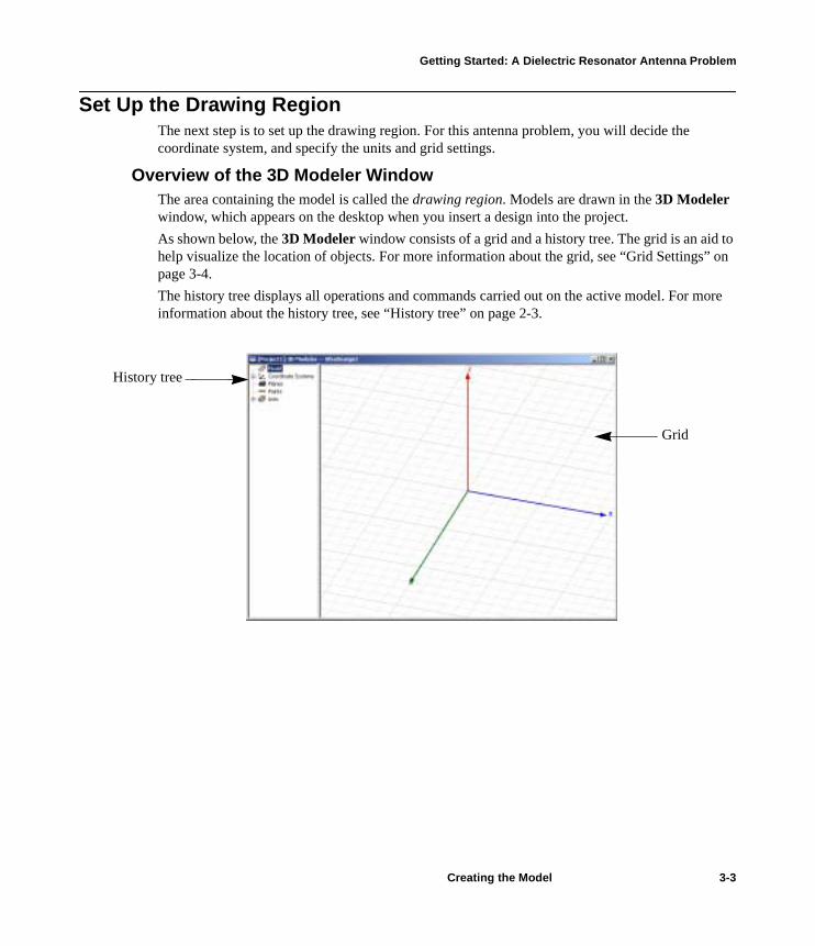
Overview of the 3D Modeler WindowThe area containing the model is called the drawing region. Models are drawn in the 3D Modeler window, which appears on the desktop when you insert a design into the project. As shown below, the 3D Modeler window consists of a grid and a history tree. The grid is an aid to help visualize the location of objects. For more information about the grid, see “Grid Settings” on page 3-4.The history tree displays all operations and commands carried out on the active model. For more information about the history tree, see “History tree” on page 2-3.
History tree
Grid
Creating the Model 3-3

Getting Started: A Dielectric Resonator Antenna Problem
Coordinate System Settings For this antenna problem, you will use the fixed, default global coordinate system (CS) as the �working CS. This is the current CS with which objects being drawn are associated.HFSS has three types of coordinate systems that let you easily orient new objects: a global �coordinate system, a relative coordinate system, and a face coordinate system. Every CS has an x-axis that lies at a right angle to a y-axis, and a z-axis that is perpendicular to the xy plane. The ori-gin (0,0,0) of every CS is located at the intersection of the x-, y-, and z-axes.
Units SettingsNow, specify the drawing units for your model. For this antenna problem, set the drawing units to millimeters. To set the units: 1. Click 3D Modeler>Units.
The Set Model Units dialog box appears.2. Select mm from the Select units menu. Make sure Rescale to new units is cleared.
If selected, the Rescale to new units option automatically rescales the grid spacing to units entered that are different than the set drawing units.
3. Click OK to accept millimeters as the units for this model.
Grid SettingsThe grid displayed in the 3D Modeler window is a drawing aid that helps to visualize the location of objects. The points on the grid are divided by their local x-, y-, and z-coordinates and grid �spacing is set according to the current project’s drawing units.For this antenna project, it is not necessary to edit any of the grid’s default properties. To edit the grid’s properties, click Grid Settings on the View menu to control the grid’s type �(cartesian or polar), style (dots or lines), density, spacing, or visibility.
Global CS The fixed, default CS for each new project. It cannot be edited or deleted.
Relative CS A user-defined CS. Its origin and orientation can be set relative to the global CS, relative to another relative CS, or relative to a geometric feature. Relative CSs enable you to easily draw objects that are located relative to other objects.
Face CS A user-defined CS. Its origin is specified on a planar object face. Face CSs enable you to easily draw objects that are located relative to an object’s face.
3-4 Creating the Model

Getting Started: A Dielectric Resonator Antenna Problem
Create the GeometryThe geometry for this dielectric resonator antenna (DRA) model consists of the five basic objects listed below with their dimensions:
Draw the Cavity The first object you will draw is the antenna’s cavity, which is created by first drawing a sphere and then splitting it into a hemispherical solid.
Draw the SphereTo draw the sphere: 1. Click Draw>Sphere, or click the Draw sphere button on the toolbar. 2. Select the center point of the sphere by entering the following values in the coordinate boxes:
3. Press the Tab key to move to the next coordinate text box.To delete the selected point and start over, press Esc.The status bar now prompts you to enter a radius for the sphere.
4. Press Enter to accept the centre point.5. Tab into the dX box and enter 25. 6. Press Enter to accept the radius value. 7. The Properties window appears. Click OK.
The sphere appears in the drawing region. 8. Press Ctrl+D to fit the sphere in the drawing region.
Air volume 30 mm radius and a height of 35 mm
Spherical Cavity 25 mm radius
Spherical DRA 12.5 mm radius
Annular ring 5.8 mm outer radius and a width of 1.0 mm.
Feed gap 1 mm thickness
X coordinate 0
Y coordinate 0
Z coordinate 0
Creating the Model 3-5
Getting Started: A Dielectric Resonator Antenna Problem
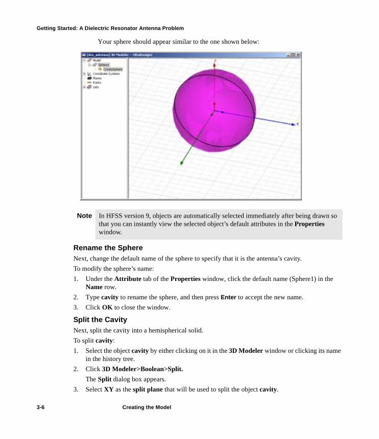
Your sphere should appear similar to the one shown below:
Rename the SphereNext, change the default name of the sphere to specify that it is the antenna’s cavity. To modify the sphere’s name:1. Under the Attribute tab of the Properties window, click the default name (Sphere1) in the
Name row.2. Type cavity to rename the sphere, and then press Enter to accept the new name. 3. Click OK to close the window.
Split the CavityNext, split the cavity into a hemispherical solid.To split cavity:1. Select the object cavity by either clicking on it in the 3D Modeler window or clicking its name
in the history tree.2. Click 3D Modeler>Boolean>Split.
The Split dialog box appears. 3. Select XY as the split plane that will be used to split the object cavity.
Note In HFSS version 9, objects are automatically selected immediately after being drawn so that you can instantly view the selected object’s default attributes in the Properties window.
3-6 Creating the Model
Getting Started: A Dielectric Resonator Antenna Problem
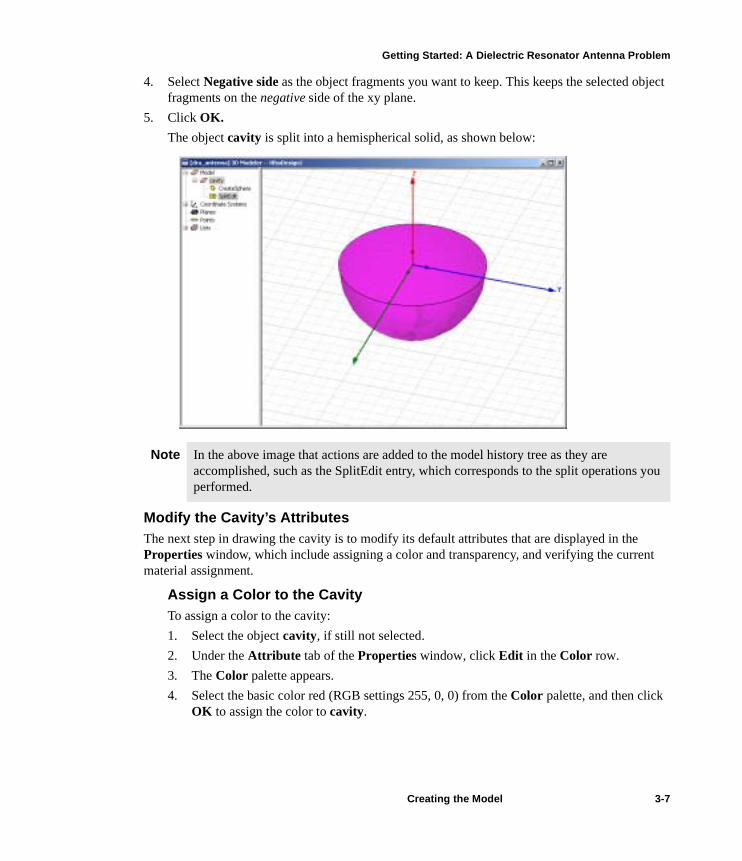
4. Select Negative side as the object fragments you want to keep. This keeps the selected object fragments on the negative side of the xy plane.
5. Click OK.The object cavity is split into a hemispherical solid, as shown below:
Modify the Cavity’s AttributesThe next step in drawing the cavity is to modify its default attributes that are displayed in the �Properties window, which include assigning a color and transparency, and verifying the current material assignment.
Assign a Color to the CavityTo assign a color to the cavity: 1. Select the object cavity, if still not selected. 2. Under the Attribute tab of the Properties window, click Edit in the Color row. 3. The Color palette appears. 4. Select the basic color red (RGB settings 255, 0, 0) from the Color palette, and then click
OK to assign the color to cavity.
Note In the above image that actions are added to the model history tree as they are accomplished, such as the SplitEdit entry, which corresponds to the split operations you performed.
Creating the Model 3-7

Getting Started: A Dielectric Resonator Antenna Problem
Assign a Transparency to the CavityTo assign a transparency level to the cavity: 1. Select the object cavity, if it is not already selected. 2. Under the Attribute tab of the Properties window, click 0 in the Transparency row.
The Set Transparency window appears. 3. Move the slider to the right to increase the transparency level, stopping on the 8th mark.
The Transparency is now set to 0.7. 4. Click outside the object, on the grid background, to deselect cavity and view the resulting
color and transparency assignments.
Verify Lighting Attributes are DisabledTo verify if the lighting attributes are disabled: 1. Click View>Modify Attributes>Lighting.
The Lighting Properties dialog box appears. 2. Verify that the Do not use lighting option is disabled. Clear this option if it is selected.
If you want, you can change the default ambient and distant light source properties at this time, though it is unnecessary for this antenna problem.
3. Click OK.
Verify the Cavity’s Material By default, all new objects created in HFSS version 9 are assigned the material vacuum. For this antenna problem, the object cavity will keep the default material assignment. There-fore, the next step is to simply verify that the cavity’s material assignment is vacuum. To verify the cavity’s material assignment: 1. Select the object cavity if it is not already selected. 2. Click the Attribute tab of the Properties window. 3. Verify that vacuum is the current material assignment, which is displayed in the Material
row. This will be the permanent material assignment for cavity.
Note HFSS version 9 lets you assign materials to objects at any time.
3-8 Creating the Model
Getting Started: A Dielectric Resonator Antenna Problem
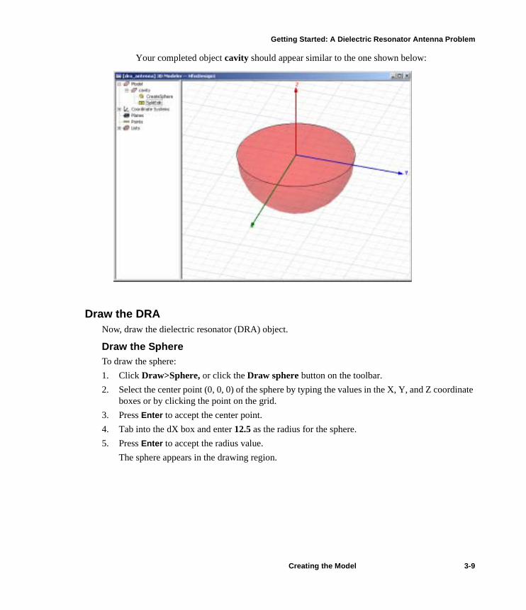
Your completed object cavity should appear similar to the one shown below:
Draw the DRANow, draw the dielectric resonator (DRA) object.
Draw the SphereTo draw the sphere:1. Click Draw>Sphere, or click the Draw sphere button on the toolbar. 2. Select the center point (0, 0, 0) of the sphere by typing the values in the X, Y, and Z coordinate
boxes or by clicking the point on the grid.3. Press Enter to accept the center point.4. Tab into the dX box and enter 12.5 as the radius for the sphere. 5. Press Enter to accept the radius value.
The sphere appears in the drawing region.
Creating the Model 3-9

Getting Started: A Dielectric Resonator Antenna Problem
The sphere should appear in your model as shown below:
Rename the SphereNext, change the default name of the sphere to specify that it is the dielectric resonator antenna (DRA) object. To modify the sphere’s name:1. Under the Attribute tab of the Properties window, click the default name (Sphere1) in the
Name row.2. Type dra to rename the sphere, and then press Enter to accept the new name.
Split the DRANext, split dra into a hemispherical solid.To split dra:1. Select dra, if not already selected. 2. Click 3D Modeler>Boolean>Split. 3. Select XY as the split plane and Positive side as the keep fragments. This keeps the selected
object fragments on the positive side of the xy plane. 4. Click OK.
3-10 Creating the Model
Getting Started: A Dielectric Resonator Antenna Problem
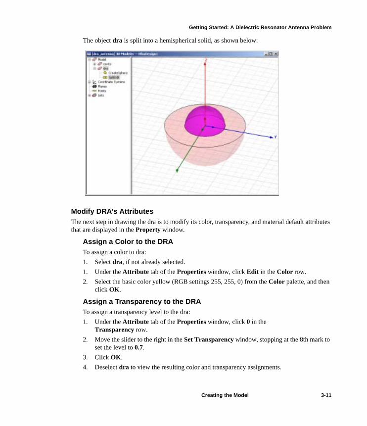
The object dra is split into a hemispherical solid, as shown below:
Modify DRA’s AttributesThe next step in drawing the dra is to modify its color, transparency, and material default attributes that are displayed in the Property window.
Assign a Color to the DRATo assign a color to dra: 1. Select dra, if not already selected. 1. Under the Attribute tab of the Properties window, click Edit in the Color row. 2. Select the basic color yellow (RGB settings 255, 255, 0) from the Color palette, and then
click OK.
Assign a Transparency to the DRATo assign a transparency level to the dra: 1. Under the Attribute tab of the Properties window, click 0 in the �
Transparency row. 2. Move the slider to the right in the Set Transparency window, stopping at the 8th mark to
set the level to 0.7. 3. Click OK.4. Deselect dra to view the resulting color and transparency assignments.
Creating the Model 3-11

Getting Started: A Dielectric Resonator Antenna Problem
Create and Assign a New Material to the DRAThe current default material assignment for the object dra is vacuum. Next, you will create a new material and assign it to dra. To create and assign a new material to the dra:1. Select dra, if not already selected. 2. Under the Attribute tab of the Properties window, click the material name in the �
Material row.The Select Definition window appears, which lists all of the materials in Ansoft’s global material library and the project’s local material library.
3. Click Add Material.
3-12 Creating the Model
Getting Started: A Dielectric Resonator Antenna Problem
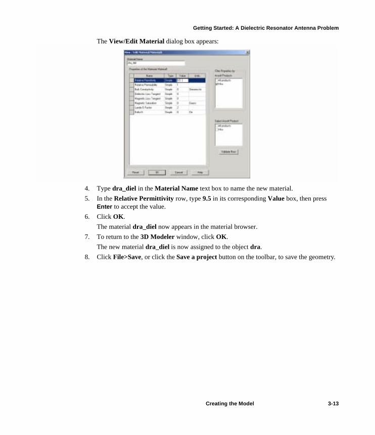
The View/Edit Material dialog box appears:
4. Type dra_diel in the Material Name text box to name the new material.5. In the Relative Permittivity row, type 9.5 in its corresponding Value box, then press
Enter to accept the value. 6. Click OK.
The material dra_diel now appears in the material browser. 7. To return to the 3D Modeler window, click OK.
The new material dra_diel is now assigned to the object dra. 8. Click File>Save, or click the Save a project button on the toolbar, to save the geometry.
Creating the Model 3-13

Getting Started: A Dielectric Resonator Antenna Problem
The completed object dra should appear in your antenna model as shown below:
Create the Annular Feed RingIn this antenna model, the annular feed ring is the controlled aperture through which the E-fields will radiate. Later on, in Chapter 4, “Setting Up the Problem”, you will assign a perfect H boundary to the annular feed ring to allow the E-fields to radiate through it. Next, you will create the antenna’s annular feed ring, which is the result of subtracting one circle from another.
Draw Circle1To draw Circle1: 1. Click Draw>Circle, or click the Draw circle button on the toolbar. 2. Select the center point (0, 0, 0) of the circle by typing the values in the coordinate boxes or by
clicking the point on the grid.3. Press Enter.4. Tab into the dX box and enter 4.8 as the radius. 5. Press Enter to accept the value.
The Properties window appears.Circle1 now appears in the model.
3-14 Creating the Model
Getting Started: A Dielectric Resonator Antenna Problem
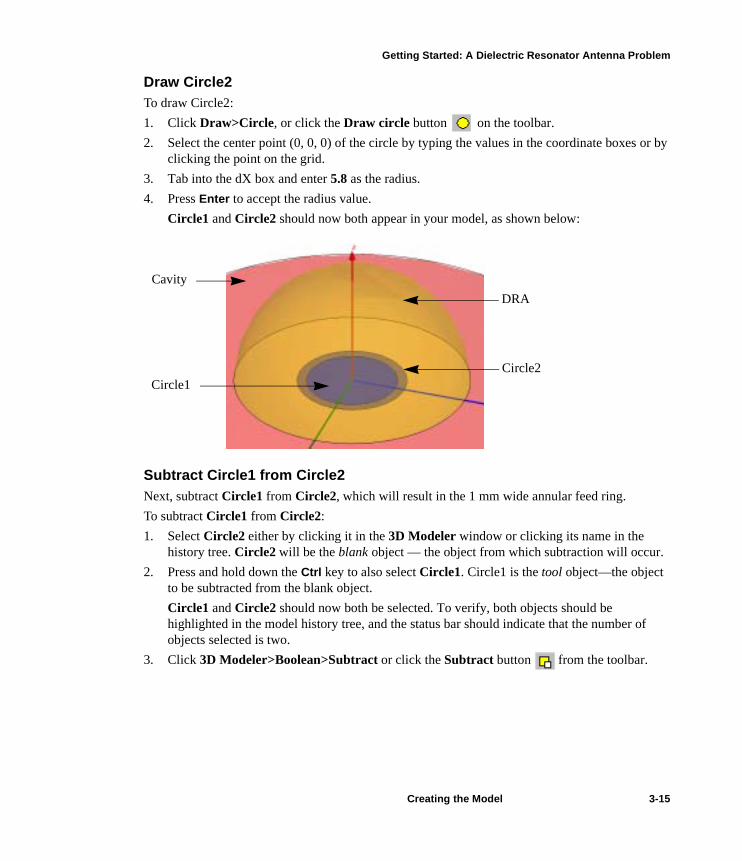
Draw Circle2To draw Circle2:1. Click Draw>Circle, or click the Draw circle button on the toolbar. 2. Select the center point (0, 0, 0) of the circle by typing the values in the coordinate boxes or by
clicking the point on the grid.3. Tab into the dX box and enter 5.8 as the radius. 4. Press Enter to accept the radius value.
Circle1 and Circle2 should now both appear in your model, as shown below:
Subtract Circle1 from Circle2Next, subtract Circle1 from Circle2, which will result in the 1 mm wide annular feed ring. To subtract Circle1 from Circle2:1. Select Circle2 either by clicking it in the 3D Modeler window or clicking its name in the �
history tree. Circle2 will be the blank object — the object from which subtraction will occur.2. Press and hold down the Ctrl key to also select Circle1. Circle1 is the tool object—the object
to be subtracted from the blank object. Circle1 and Circle2 should now both be selected. To verify, both objects should be �highlighted in the model history tree, and the status bar should indicate that the number of objects selected is two.
3. Click 3D Modeler>Boolean>Subtract or click the Subtract button from the toolbar.
CavityDRA
Circle2Circle1
Creating the Model 3-15
Getting Started: A Dielectric Resonator Antenna Problem
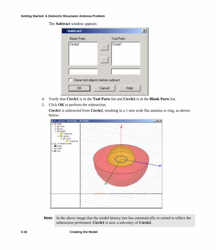
The Subtract window appears:
4. Verify that Circle1 is in the Tool Parts list and Circle2 is in the Blank Parts list. 5. Click OK to perform the subtraction.
Circle1 is subtracted from Circle2, resulting in a 1 mm wide flat annulus or ring, as shown below:
Note In the above image that the model history tree has automatically re-sorted to reflect the subtraction performed. Circle1 is now a sub-entry of Circle2.
3-16 Creating the Model

Getting Started: A Dielectric Resonator Antenna Problem
Rename Circle2Next, change the name of Circle2 to specify that it is the antenna’s annular feed ring.To modify the name of Circle2:1. Under the Attribute tab in the Properties window, click Circle2 in the Name row. 2. Type annular_rng to rename the circle, and then press Enter to accept the new name.
Modify the Annular Feed Ring’s AttributesThe next step to drawing the annular feed ring is to modify its color and transparency. The annular feed ring is a sheet object, which has surface area but no volume. Since the material parameter is a volumetric assignment, the annular feed ring will not have a material assignment.
Assign a Color to the Annular Feed Ring To assign a color to the annular feed ring: 1. Under the Attribute tab in the Properties window, click Edit in the Color row.2. Select the basic color dark blue (RGB settings 0, 0, 128) from the Color palette, and then
click OK.
Verify Annular Feed Ring’s Transparency The annular feed ring object will keep the default transparency assignment. Therefore, you simply have to verify its default transparency assignment. To assign a transparency to the annular feed ring: 1. Under the Attribute tab in the Properties window, click 0 in the Transparency row. 2. Move the slider to the right in the Set Transparency window and stop at the 10th mark to
set the level at 0.9. 3. Click OK.
Deselect annular_rng to view the resulting color and transparency assignments.
Creating the Model 3-17
Getting Started: A Dielectric Resonator Antenna Problem
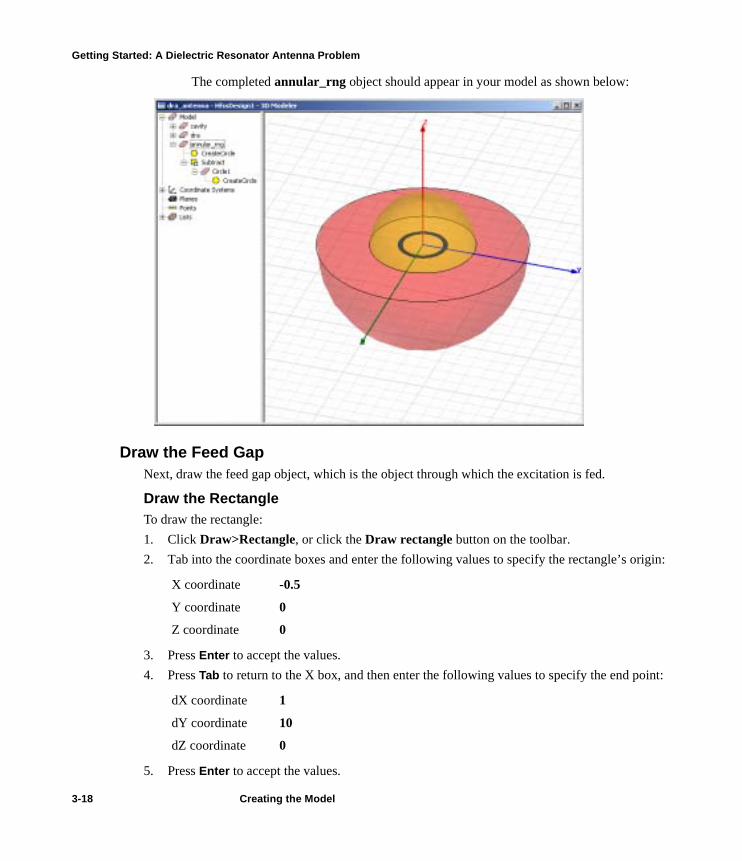
The completed annular_rng object should appear in your model as shown below:
Draw the Feed Gap Next, draw the feed gap object, which is the object through which the excitation is fed.
Draw the RectangleTo draw the rectangle:1. Click Draw>Rectangle, or click the Draw rectangle button on the toolbar. 2. Tab into the coordinate boxes and enter the following values to specify the rectangle’s origin:
3. Press Enter to accept the values.4. Press Tab to return to the X box, and then enter the following values to specify the end point:
5. Press Enter to accept the values.
X coordinate -0.5
Y coordinate 0
Z coordinate 0
dX coordinate 1
dY coordinate 10
dZ coordinate 0
3-18 Creating the Model

Getting Started: A Dielectric Resonator Antenna Problem
The Properties window appears.The rectangle appears in the model as shown below:
Intersect the Rectangle and the Annular Feed RingNext, you will intersect the rectangle and the annular feed ring to produce the antenna’s feed gap. To intersect the rectangle and the annular feed ring: 1. Click Tools > Options > 3D Modeler Options.
The 3D Modeler Options dialog box appears. 2. Click the Operation tab. 3. Under Clone, select Clone tool objects before intersect, and then click OK to activate.
This option instructs HFSS to always keep a copy of the original objects that intersect the first object selected.
4. Select the object Rectangle1, if not already selected. 5. Press and hold down Ctrl to also select the object annular_rng.
The objects Retangle1 and annular_rng should now both be selected. 6. Click 3D Modeler > Boolean > Intersect, or click the Intersect button from the toolbar, to
perform the intersection.
Rectangle
Creating the Model 3-19
Getting Started: A Dielectric Resonator Antenna Problem
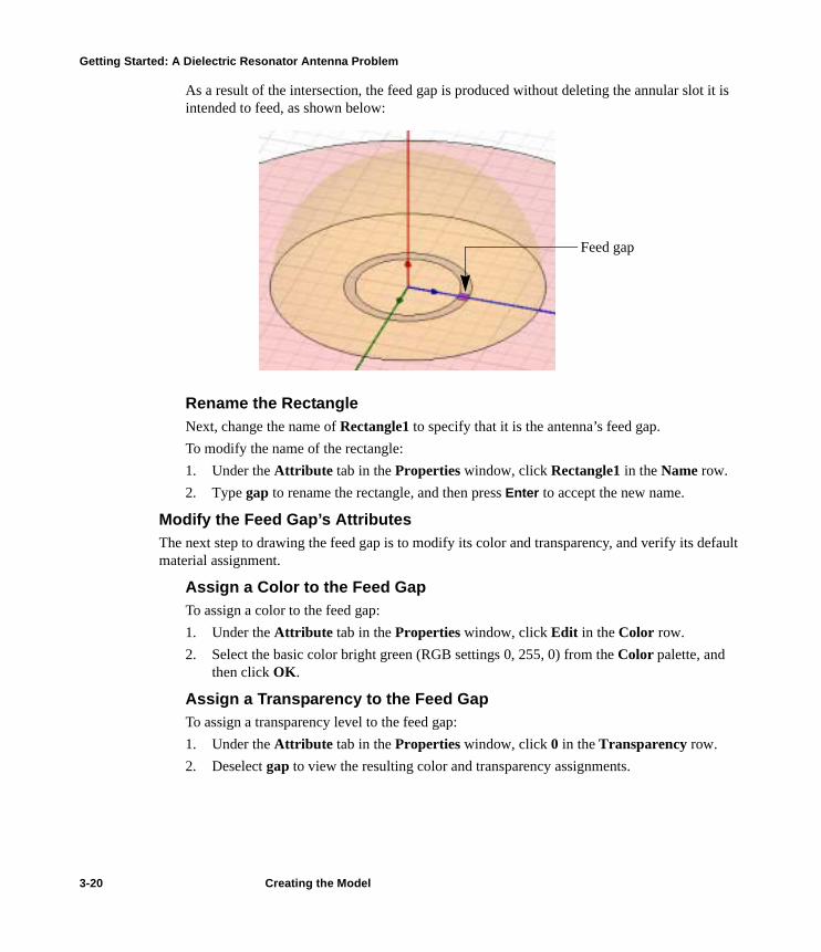
As a result of the intersection, the feed gap is produced without deleting the annular slot it is intended to feed, as shown below:
Rename the RectangleNext, change the name of Rectangle1 to specify that it is the antenna’s feed gap.To modify the name of the rectangle: 1. Under the Attribute tab in the Properties window, click Rectangle1 in the Name row. 2. Type gap to rename the rectangle, and then press Enter to accept the new name.
Modify the Feed Gap’s AttributesThe next step to drawing the feed gap is to modify its color and transparency, and verify its default material assignment.
Assign a Color to the Feed GapTo assign a color to the feed gap: 1. Under the Attribute tab in the Properties window, click Edit in the Color row.2. Select the basic color bright green (RGB settings 0, 255, 0) from the Color palette, and
then click OK.
Assign a Transparency to the Feed GapTo assign a transparency level to the feed gap: 1. Under the Attribute tab in the Properties window, click 0 in the Transparency row. 2. Deselect gap to view the resulting color and transparency assignments.
Feed gap
3-20 Creating the Model

Getting Started: A Dielectric Resonator Antenna Problem
Draw the Air VolumeTo analyze radiation effects, you must create a virtual object that represents the radiation boundary. For this antenna model, you will create a radiation-transparent air volume surface sufficiently far from the model. Next, you will draw a regular polyhedron with 18 segments to represent this virtual object. Then, in Chapter 4, Setting Up the Problem, you will assign a radiation boundary to this object.
Draw the PolyhedronTo draw the polyhedron:1. Click Draw>Regular Polyhedron, or click the Draw regular polyhedron button on the�
toolbar. 2. Select the center point (0, 0, 0) of the circle by typing the values in the coordinate boxes or by
clicking the point on the grid.3. Tab into the dX box and enter a radius value of 30, and then press Enter to accept the value.
The status bar now prompts you to enter a height for the polyhedron. 4. Tab into the dZ coordinate box and enter a height value of 35, and then press Enter to accept
the value. The Segment Number window appears.
Creating the Model 3-21

Getting Started: A Dielectric Resonator Antenna Problem
5. Toggle the Up arrow to set the number of segments to 18, and then click OK to accept the value. The Properties window appears. The polyhedron is drawn.
Rename the PolyhedronNext, change the name of Polyhedron1 to specify that it is the antenna’s air volume.To modify the name of the polyhedron: 1. Under the Attribute tab in the Properties window, click the name Regular Polyhedron1 in
the Name row. 2. Type airvol to rename the polyhedron, and then press Enter to accept the new name.
Modify the Air Volume’s AttributesThe next step to drawing the air volume is to modify its color and transparency, and verify its default material assignment.
Assign a Color to the Air VolumeTo assign a color to the air volume: 1. Under the Attribute tab in the Properties window, click Edit in the Color row.2. Select the basic color light blue (RGB settings 0, 255, 255) from the Color palette, and
then click OK.
Assign a Transparency to the Air VolumeTo assign a transparency level to the air volume: 1. Under the Attribute tab in the Properties window, click the default value 0 in the �
Transparency row. 2. Move the slider to the right in the Set Transparency window and stop at the 2nd mark to
set the level at 0.1. Deselect airvol to view the resulting color and transparency assignments.
Verify Air Volume’s MaterialThe object airvol will keep the default material assignment vacuum. To verify the air volume’s material assignment:1. Select airvol.2. Under the Attribute tab of the Properties window, verfiy that vacuum is the current �
material assignment, which is displayed in the Material row. 3. Click File>Save, or click the Save a project button on the toolbar, to save the geometry.
3-22 Creating the Model

Getting Started: A Dielectric Resonator Antenna Problem
The completed airvol object should appear in your model as shown below:
Split the Model for SymmetryThis model as constructed is symmetrical about the yz plane. Now, split the model along the yz plane for symmetry.To split the model and create a cut plane:1. Click Edit > Select All to select all the objects of the model. 2. Click 3D Modeler > Boolean > Split, or click the Split button on the toolbar.
The Split window appears. 3. Select YZ as the split plane and Positive side as the keep fragments. 4. Click OK to split the entire model.
Creating the Model 3-23

Getting Started: A Dielectric Resonator Antenna Problem
Your final model should appear similar to the one shown below:
5. Click File > Save, or click the Save a project button on the toolbar, to save the final geometry. �You are now ready to assign ports and boundaries to your antenna model.
3-24 Creating the Model

Setting Up the Problem
Now that you have created the geometry and assigned all materials for the antenna problem, you are ready to define its ports and boundaries.Your goals for this chapter are to:• Define the boundary conditions, such as the location of a radiation boundary and the symmetry
plane.• Define the lumped port through which the signal (voltage) enters the antenna.• Verify that you correctly assigned the boundaries and excitations to the model.Now you are ready to set up the problem.
Time It should take you approximately 30 minutes to work through this chapter.
Setting Up the Problem 4-1
Getting Started: A Dielectric Resonator Antenna Problem
Set Up Boundaries and Excitations Now that you have created all the objects of the antenna model and defined their properties, you must define the boundary and excitation conditions. These conditions specify the excitation signals �entering the structure, the behavior of electric and magnetic fields at various surfaces in the model, and any special surface characteristics.
Boundary ConditionsBoundaries specify the behavior of magnetic and electric fields at various surfaces. They can also be used to identify special surfaces —such as resistors— whose characteristics differ from the default.The following four types of boundary conditions will be used for this antenna problem:
Excitation ConditionsPorts define surfaces exposed to non-existent materials (generally the background or materials defined to be perfect conductors) through which excitation signals enter and leave the structure.One lumped port will be defined for this antenna problem. Lumped ports are similar to traditional wave ports, but can be located internally and have a complex user-defined impedance. Lumped ports compute S-parameters directly at the port. A lumped port can be defined as a rectangle from the edge of the trace to the ground, as in this antenna problem, or as a traditional wave port. The default boundary is perfect H on all edges that do not come in contact with the metal.
Radiation This type of boundary simulates an open problem that allows waves to radiate infinitely far into space, such as antenna designs. HFSS absorbs the wave at the radiation boundary, essentially ballooning the boundary infinitely far away from the structure. In this antenna model, the air volume object is defined as a radiation boundary.
Perfect E This type of boundary models a perfectly conducting surface in a structure, which forces the electric filed to be normal to the surface. In this antenna model, the bottom face of the air volume object is defined as a perfect E boundary.
Perfect H This type of boundary forces the tangential component of the H-field to be the same on both sides of the boundary. In this antenna model, the annular feed ring is the aperture that is assigned this boundary. Because the aperture is defined as a perfect H boundary, the E-fields will radiate through it. If it was not defined as a perfect H boundary, the E-field would not radiate through and the signal would terminate at the aperture.
Symmetry In structures that have an electromagnetic plane of symmetry, such as this antenna model, the problem can be simplified by modeling only one-half of the model and identifying the exposed surface as a perfect H or perfect E boundary. For this antenna problem, a perfect H symmetry boundary is used.
4-2 Setting Up the Problem
Getting Started: A Dielectric Resonator Antenna Problem
Assigning BoundariesFirst, you will assign all boundary conditions to the model. For information on the types of boundaries you will assign, see “Boundary Conditions” on page 4-2.
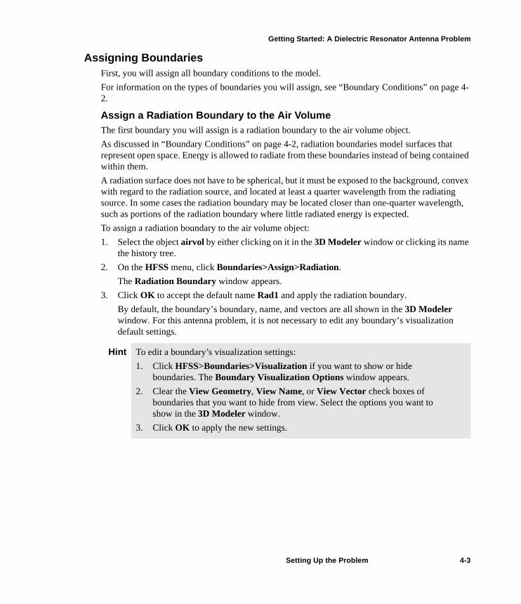
Assign a Radiation Boundary to the Air VolumeThe first boundary you will assign is a radiation boundary to the air volume object. As discussed in “Boundary Conditions” on page 4-2, radiation boundaries model surfaces that �represent open space. Energy is allowed to radiate from these boundaries instead of being contained within them. A radiation surface does not have to be spherical, but it must be exposed to the background, convex with regard to the radiation source, and located at least a quarter wavelength from the radiating source. In some cases the radiation boundary may be located closer than one-quarter wavelength, such as portions of the radiation boundary where little radiated energy is expected.To assign a radiation boundary to the air volume object: 1. Select the object airvol by either clicking on it in the 3D Modeler window or clicking its name
the history tree.2. On the HFSS menu, click Boundaries>Assign>Radiation.
The Radiation Boundary window appears. 3. Click OK to accept the default name Rad1 and apply the radiation boundary.
By default, the boundary’s boundary, name, and vectors are all shown in the 3D Modeler �window. For this antenna problem, it is not necessary to edit any boundary’s visualization default settings.
Hint To edit a boundary’s visualization settings:1. Click HFSS>Boundaries>Visualization if you want to show or hide
boundaries. The Boundary Visualization Options window appears.2. Clear the View Geometry, View Name, or View Vector check boxes of
boundaries that you want to hide from view. Select the options you want to show in the 3D Modeler window.
3. Click OK to apply the new settings.
Setting Up the Problem 4-3

Getting Started: A Dielectric Resonator Antenna Problem
The resulting radiation boundary is applied to the object airvol and now appears as a subentry of Boundaries in the project tree, as shown below:
Assign a Perfect E Boundary to the Air VolumeNext, define the intersection between the cavity and the air volume as a perfect E boundary �condition. Therefore, you will assign a perfect E boundary to the bottom face of the air volume object, which will be the ground plane of the antenna. By default, all HFSS model surfaces exposed to the background are assumed to have perfect E boundaries; HFSS assumes that the entire structure is surrounded by perfectly conducting walls. The electric field is assumed to be normal to these surfaces. The final field solution must match the case in which the tangential component of the electric field goes to zero at perfect E boundaries.The surfaces of all model objects that have been assigned perfectly conducting materials are auto-matically assigned perfect E boundaries.
Radiation boundary added as a subentry of Boundaries.
Radiation boundary applied to the air volume object.
Properties of the Radiation boundary
4-4 Setting Up the Problem

Getting Started: A Dielectric Resonator Antenna Problem
To assign a perfect E boundary to the bottom face of the air volume object: 1. Deselect the radiation boundary you just assigned, if it is still selected. 2. Right-click in the 3D Modeler window, then click Select Faces on the shortcut menu.
In this mode you can select an object’s faces instead of the entire object.When the mouse hovers over a face in the 3D Modeler window, that face is highlighted, which indicates that it will be selected when you click.
3. Select the bottom face of the object airvol by doing the following: • Press and hold down Alt and drag the mouse to rotate the model to a position where you
can then click the bottom face of the object airvol. If you are having difficulty selecting this interior bottom face, right-click in the �3D Modeler window and click Next Behind from the shortcut menu. This option selects the face or object behind a selected face or object.
In the figure below, the bottom face of airvol is selected and highlighted:
4. On the HFSS menu, click Boundaries>Assign>Perfect E.
Setting Up the Problem 4-5

Getting Started: A Dielectric Resonator Antenna Problem
The Perfect E Boundary window appears.
5. Clear Infinite Ground Plane if it is selected. If selected, the Infinite Ground Plane option simulates the effects of an infinite ground plane. This option only affects the calculation of near- and far-field radiation during post processing. The 3D Post Processor models the boundary as a finite portion of an infinite, perfectly �conducting plane.
6. Click OK to accept the default name PerfE1 and apply the perfect E boundary. The resulting perfect E boundary condition is assigned to the bottom face of the object airvol, as shown below:
Hint You can also assign boundaries by selecting the object or object face to which you want to assign the boundary, and then doing one of the following:• Right-click in the 3D Modeler window, point to Assign Boundary, and then click
the boundary type you want to assign. Right-click on Boundaries in the project tree, point to Assign, and then click the boundary type you want to assign.
In the above image that boundaries are listed alphabetically in the project tree and re-ordered as new ones are added.
4-6 Setting Up the Problem
Getting Started: A Dielectric Resonator Antenna Problem
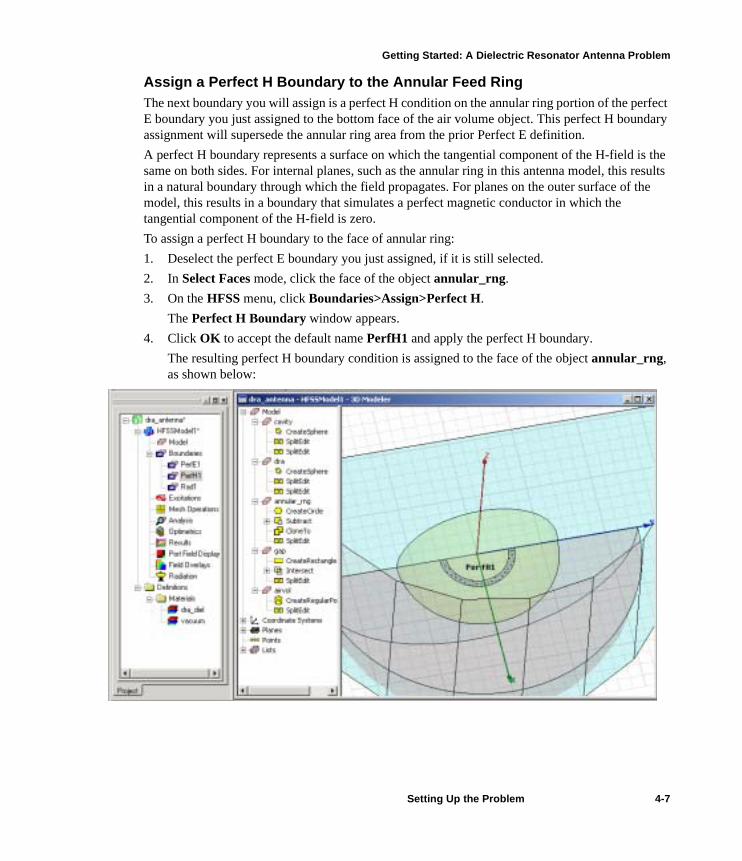
Assign a Perfect H Boundary to the Annular Feed Ring The next boundary you will assign is a perfect H condition on the annular ring portion of the perfect E boundary you just assigned to the bottom face of the air volume object. This perfect H boundary assignment will supersede the annular ring area from the prior Perfect E definition. A perfect H boundary represents a surface on which the tangential component of the H-field is the same on both sides. For internal planes, such as the annular ring in this antenna model, this results in a natural boundary through which the field propagates. For planes on the outer surface of the model, this results in a boundary that simulates a perfect magnetic conductor in which the �tangential component of the H-field is zero.To assign a perfect H boundary to the face of annular ring: 1. Deselect the perfect E boundary you just assigned, if it is still selected.2. In Select Faces mode, click the face of the object annular_rng. 3. On the HFSS menu, click Boundaries>Assign>Perfect H.
The Perfect H Boundary window appears.4. Click OK to accept the default name PerfH1 and apply the perfect H boundary.
The resulting perfect H boundary condition is assigned to the face of the object annular_rng, as shown below:
Setting Up the Problem 4-7

Getting Started: A Dielectric Resonator Antenna Problem
Assign a Symmetry Boundary to the ModelHFSS has a boundary condition specifically for symmetry planes. Instead of defining a perfect E or perfect H boundary, you define a perfect E or perfect H symmetry plane. When you are defining a symmetry plane, you must decide which type of symmetry boundary should be used, a perfect E or a perfect H. In general, use the following guidelines to decide which type of symmetry plane to use: • If the symmetry is such that the E-field is normal to the symmetry plane, use a perfect E �
symmetry plane. • If the symmetry is such that the E-field is tangential to the symmetry plane, use a perfect H
symmetry plane.The simple two-port rectangular waveguide shown below illustrates the differences between the two types of symmetry planes. The E-field of the dominant mode signal (TE10) is shown. The waveguide has two planes of symmetry, one vertically through the center and one horizontally.• The horizontal plane of symmetry is a perfect E surface. The E-field is normal and the H-field
is tangential to that surface.• The vertical plane of symmetry is a perfect H surface. The E-field is tangential and H-field is �
normal to that surface.
Since the antenna model in this guide has a vertical plane of symmetry and the E-field is tangential to the surface, use a perfect H boundary for the symmetry plane. Next, you will assign a perfect H symmetry boundary to the symmetry cut faces of the objects �airvol and cavity (the model’s symmetry plane).
Electric field of TE10 Mode
Perfect E symmetry plane
Perfect H symmetry plane
4-8 Setting Up the Problem
Getting Started: A Dielectric Resonator Antenna Problem
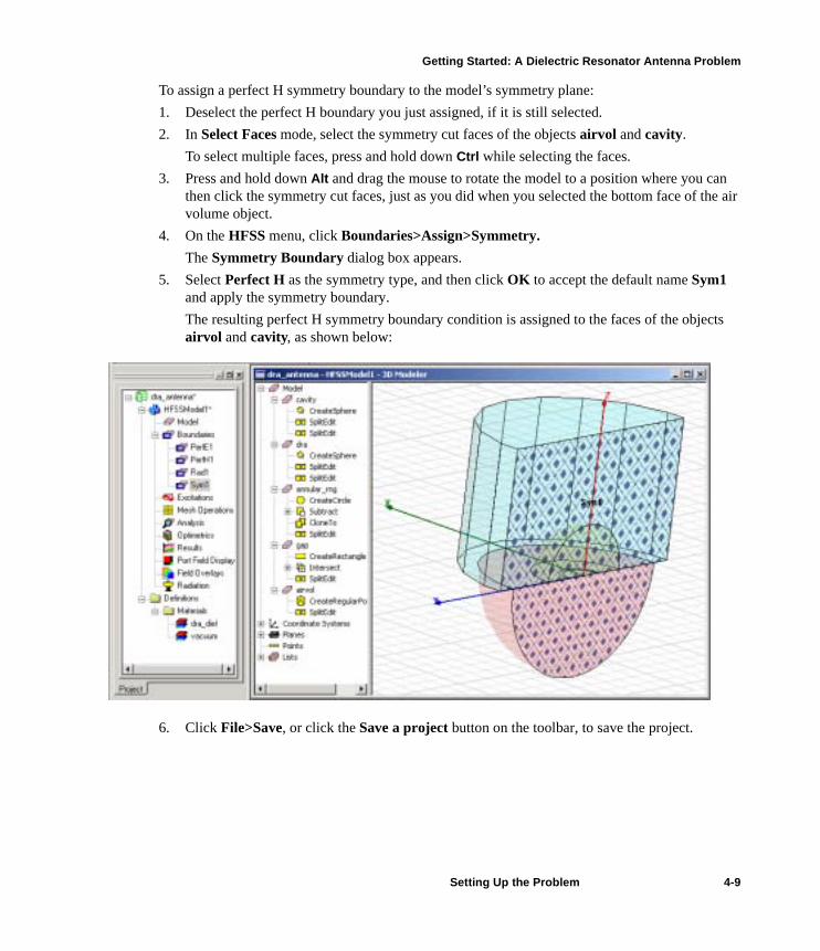
To assign a perfect H symmetry boundary to the model’s symmetry plane: 1. Deselect the perfect H boundary you just assigned, if it is still selected.2. In Select Faces mode, select the symmetry cut faces of the objects airvol and cavity.
To select multiple faces, press and hold down Ctrl while selecting the faces. 3. Press and hold down Alt and drag the mouse to rotate the model to a position where you can
then click the symmetry cut faces, just as you did when you selected the bottom face of the air volume object.
4. On the HFSS menu, click Boundaries>Assign>Symmetry. The Symmetry Boundary dialog box appears.
5. Select Perfect H as the symmetry type, and then click OK to accept the default name Sym1 and apply the symmetry boundary.The resulting perfect H symmetry boundary condition is assigned to the faces of the objects airvol and cavity, as shown below:
6. Click File>Save, or click the Save a project button on the toolbar, to save the project.
Setting Up the Problem 4-9
Getting Started: A Dielectric Resonator Antenna Problem
Assigning ExcitationsNow you will assign all excitation conditions to the model. For information on the types of excitations you will assign, see “Excitation Conditions” on page 4-2.
Assign a Lumped Port Across the GapFor this antenna problem, the engineering focus is on the behavior of the antenna itself, not its feed. Therefore, the model will feed with a lumped port across the annular slot, or gap object. Lumped ports are similar to traditional wave ports, but can be located internally and have a �complex user-defined impedance. Lumped ports compute S-parameters directly at the port. A lumped port can be defined as a rectangle from the edge of the trace to the ground, as in this antenna problem, or as a traditional wave port. The default boundary is perfect H on all edges that do not come in contact with the metal.
To assign a lumped port across the gap object: 1. Deselect the perfect H symmetry boundary you just assigned, if it is still selected. 2. Click View > Zoom In to zoom in on the area where the gap object is located. 3. In Select Faces mode, select the face of gap.4. On the HFSS menu, click Excitations>Assign>Lumped Port.
The Lumped Port wizard appears.The first time you assign a lumped port, HFSS version 9 walks you through the process with a step-by-step wizard.
5. In the Lumped Port:General step, enter the values listed below, and then click Next.
6. In the Lumped Port:Modes step, click in the Integration Line list, and then select New Line. 7. The Lumped Port wizard disappears while you draw the vector.8. Define the integration line:
a. Select the start point by clicking the point where the outside of the gap and the y axis �intersect (0,5.8, 0).
b. Select the end point by clicking the point where the inside of the gap and the y axis �intersect (0,4.8, 0). The endpoint defines the direction and length of the integration line. The Lumped Port wizard reappears.
Note The setup of a lumped port varies slightly depending on whether the solution is modal or terminal. As a reminder, the solution type for this antenna problem is modal driven.
Name LumpPort1 The name of the port.
Resistance 100 Ohms The resistance, or real port impedance.
Reactance 0 Ohms The reactance, or imaginary port impedance.
4-10 Setting Up the Problem
Getting Started: A Dielectric Resonator Antenna Problem
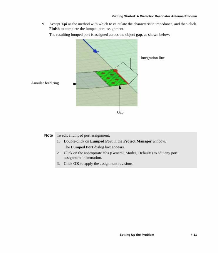
9. Accept Zpi as the method with which to calculate the characteristic impedance, and then click Finish to complete the lumped port assignment.The resulting lumped port is assigned across the object gap, as shown below:
Note To edit a lumped port assignment:1. Double-click on Lumped Port in the Project Manager window.
The Lumped Port dialog box appears. 2. Click on the appropriate tabs (General, Modes, Defaults) to edit any port
assignment information.3. Click OK to apply the assignment revisions.
Integration line
Gap
Annular feed ring
Setting Up the Problem 4-11
Getting Started: A Dielectric Resonator Antenna Problem
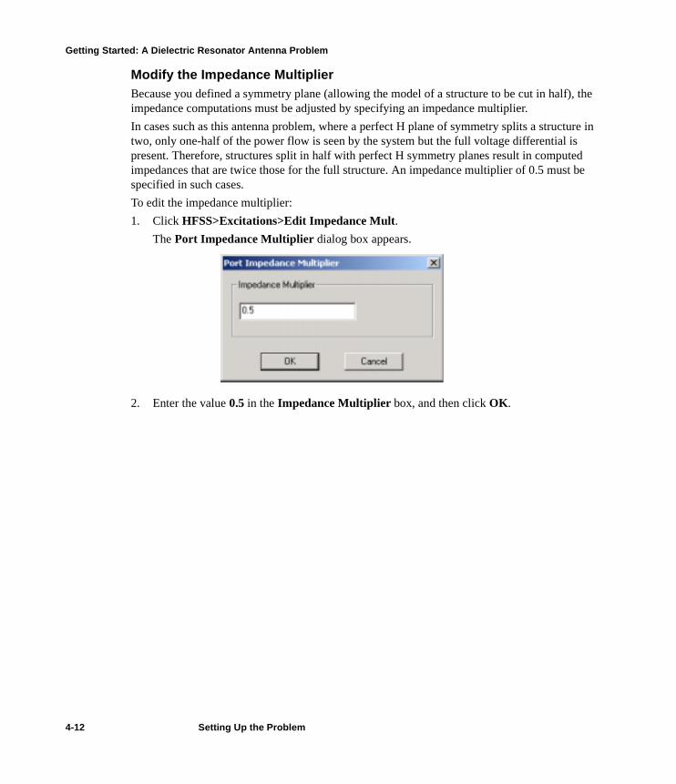
Modify the Impedance MultiplierBecause you defined a symmetry plane (allowing the model of a structure to be cut in half), the impedance computations must be adjusted by specifying an impedance multiplier.In cases such as this antenna problem, where a perfect H plane of symmetry splits a structure in two, only one-half of the power flow is seen by the system but the full voltage differential is present. Therefore, structures split in half with perfect H symmetry planes result in computed impedances that are twice those for the full structure. An impedance multiplier of 0.5 must be �specified in such cases.To edit the impedance multiplier:1. Click HFSS>Excitations>Edit Impedance Mult.
The Port Impedance Multiplier dialog box appears.
2. Enter the value 0.5 in the Impedance Multiplier box, and then click OK.
4-12 Setting Up the Problem

Getting Started: A Dielectric Resonator Antenna Problem
Verify All Boundary and Excitation AssignmentsNow that you have assigned all the necessary boundaries and excitations to the model, you should review their specific locations on the model in the solver view. When you verify boundaries and excitations in the solver view, you review the locations of the boundaries and excitations as you have defined them for generating a solution (solving). HFSS runs an initial mesh and determines the locations of the boundaries and excitations on the model. Then, you can select a boundary or excitation from the list in the Boundary Display (Solver View) window to view its highlighted area in the model. To check the solver’s view of boundaries and excitations: 1. Click HFSS>Boundary Display (Solver View).
HFSS runs an initial mesh and determines the locations of the boundaries and excitations on the model. The Solver View of Boundaries window appears, which lists all the boundaries and �excitations for the active model in the order in which they were assigned.
2. Select a check box in the Visibility column that corresponds with the boundary or excitaton for which you want to review its location on the model. The selected boundary or excitation will appear in the model in the color it has been assigned, as indicated in the Color column. • Visible to Solver will appear in the Solver Visibility column for each boundary that is
valid. • Overridden will appear in the Solver Visibility column for each boundary or excitation
that overwrites any existing boundary or excitation with which it overlaps. 3. Verify that the boundaries or excitations you assigned to the model are being displayed as you
intended for solving purposes. 4. Modify the parameters for those boundaries or excitations that are not being displayed �
as you intended.
Setting Up the Problem 4-13

Getting Started: A Dielectric Resonator Antenna Problem
5. Click Close, and then click File>Save, or click the Save a project button on the toolbar, to save the geometry.
You are now ready to set up the solution parameters for this antenna problem and generate �a solution.
Warning Be sure to save geometric models periodically; HFSS does not automatically save models. Saving frequently helps prevent the loss of your work if a problem occurs.
4-14 Setting Up the Problem

Generating A Solution
Now that you have created the geometry and set up the model, you are ready to generate a solution.Your goals for this chapter are to:• Set up the solution parameters that will be used in calculating the solution.• Define meshing instructions.• Validate the project setup. • Generate a solution. • View the solution data, such as convergence and matrix data information.
Generating A Solution 5-1

Getting Started: A Dielectric Resonator Antenna Problem
Specify Solution OptionsBefore you can generate a solution, you need to specify the solution parameters. This controls how HFSS computes the requested solution. Each solution setup includes the following information:• General data about the solution’s generation.• Adaptive mesh refinement parameters, if you want the mesh to be refined iteratively in areas of
highest error.• Frequency sweep parameters, if you want to solve over a range of frequencies.You can define more than one solution setup per design; however, you will define only one solution setup for this antenna problem.
Add a Solution SetupNow, you will specify how HFSS will compute the solution by adding a solution setup to the antenna project’s design. To add a solution setup to the design: 1. Click HFSS>Analysis>Add Solution Setup.
The Solution Setup dialog box appears:
5-2 Generating A Solution
Getting Started: A Dielectric Resonator Antenna Problem
It is divided into the following tabs:
2. Click the General tab, and specify the following: a. Enter these values:
b. Accept all remaining current default settings. 3. Click the Advanced tab, and specify the following:
a. Select Do Lambda Refinement.Lambda refinement is the process of refining the initial mesh based on the material-�dependent wavelength. It is recommended and selected by default.
General Includes general solution settings.
Advanced Includes advanced settings for initial mesh generation and adaptive analysis.
Ports Includes mesh generation options for model ports.This tab only appears if a port was defined.
Defaults Enables you to save the current settings as the defaults for future solution setups or revert the current settings to HFSS’s standard settings.
Solution Frequency
3.75 GHz
For every modal driven solution setup, you must specify the frequency at which to generate the solution. For this antenna model, you will solve over a range of frequencies, which will require you to define a frequency sweep in “Add a Frequency Sweep to the Solution Setup” on page 5-5. If a frequency sweep is solved, an adaptive analysis is performed only at the solution frequency.
Max. Number of Passes
15
The Maximum Number of Passes value is the maximum number of mesh refinement cycles that you would like HFSS to perform. This value is a stopping criterion for the adaptive solution; if the maximum number of passes has been completed, the adaptive analysis stops. If the maximum number of passes has not been completed, the adaptive analysis will continue unless the convergence criteria are reached.
Max Delta S Per Pass
0.005
The delta S is the change in the magnitude of the S-parameters between two consecutive passes. The value you set for Maximum Delta S Per Pass is a stopping criterion for the adaptive solution. If the magnitude and phase of all S-parameters change by an amount less than this value from one iteration to the next, the adaptive analysis stops. Otherwise, it continues until the requested number of passes is completed.
Generating A Solution 5-3
Getting Started: A Dielectric Resonator Antenna Problem
b. Enter 0.25 in the Target text box. This value specifies the size of wavelength by which HFSS will refine the mesh.
c. Enter 2 in the Minimum Converged Passes text box. This value specifies the least number of passes for which the convergence criteria must be met before the adaptive analysis will stop.
d. Accept all remaining current default settings. 4. Click the Ports tab, and specify the following:
a. Clear Automatically Set Min/Max Triangles, if it is selected.If selected, HFSS will determine the reasonable values for the minimum and maximum number of triangles based on the port’s setup.
b. Enter 40 in the Minimum Number of Triangles text box. The mesh for each model port will be adaptively refined until it includes the minimum number of triangles you specified. Refinement will then continue until the port field �accuracy or the maximum number of triangles (500) is reached.
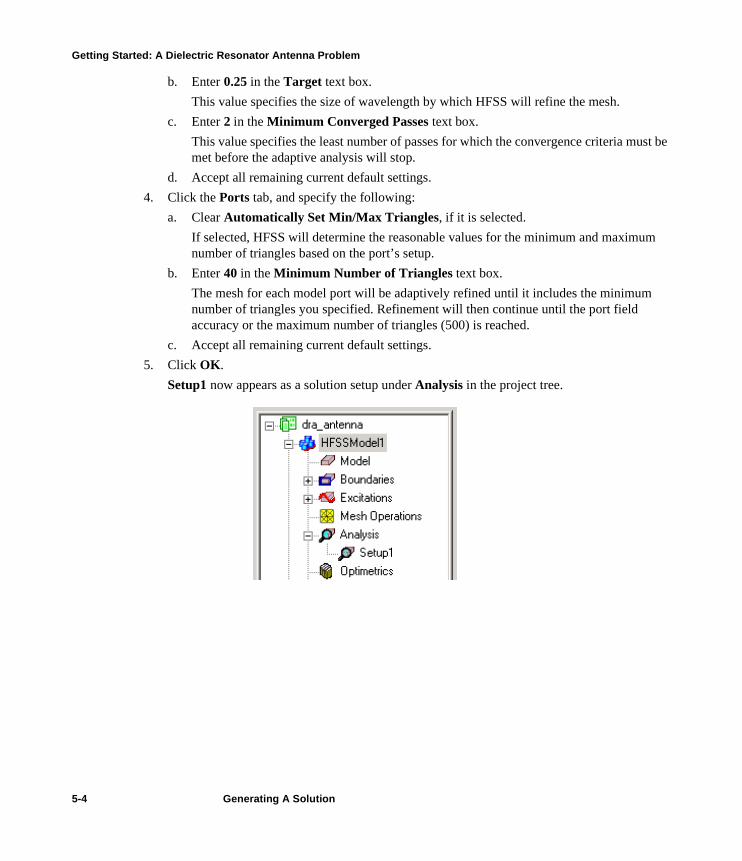
c. Accept all remaining current default settings. 5. Click OK.
Setup1 now appears as a solution setup under Analysis in the project tree.
5-4 Generating A Solution

Getting Started: A Dielectric Resonator Antenna Problem
Add a Frequency Sweep to the Solution SetupTo generate a solution across a range of frequencies, add a frequency sweep to the solution setup. HFSS performs the sweep after the adaptive solution.For this antenna model, you will add a Fast frequency sweep to the solution setup. A Fast sweep generates a unique full-field solution for each division within a frequency range. It is best for mod-els that will abruptly resonate or change operation in the frequency band, and obtains an accurate representation of the behavior near the resonance.To add a fast frequency sweep:1. Click HFSS>Analysis Setup>Add Sweep.
The Select window appears. 2. Select Setup1 for the solution setup to which the sweep applies, and click OK.
The Edit Sweep dialog box appears.
3. Under the Sweep Type section, select Fast as the frequency sweep type you want to add. 4. Verify Linear Step is selected as the Type.5. Under the Frequency Setup section, enter these values to define the sweep:
Start 2.5 GHz
Stop 5 GHz
Step Size 0.01 GHz
Generating A Solution 5-5
Getting Started: A Dielectric Resonator Antenna Problem
6. Select Save Fields, which saves the 3D field solutions associated with all port modes at each �frequency.
7. Click Display if you want to display each of the sweep values at the 0.01 GHz step size �increment within the frequency range you specified.
8. Click OK. Sweep1 now appears as a frequency sweep under Setup1 in the project tree.
Define Mesh OperationsIn HFSS, mesh operations are optional mesh refinement settings that are specified before a mesh is generated. The technique of providing HFSS with mesh construction guidance is referred to as “seeding” the mesh. Since the fields in the annular feed ring are very important in this antenna model, you will provide some meshing instructions on the faces of this object. You will assign a length-based mesh refinement to the faces of the annular feed ring. Requesting length-based mesh refinement instructs HFSS to refine the length of tetrahedral elements until they are below a specified value. The length of a tetrahedron is defined as the length of its longest edge.You specify the maximum length of tetrahedra on faces or inside of objects. You can also specify the maximum number of elements that are added during the refinement. When the mesh is �generated, the refinement criteria you specified will be used.To assign a length-based mesh refinement to all the faces of the annular feed ring: 1. Select the object annular_rng. 2. On the HFSS menu, point to Mesh Operations>Assign>On Selection, and then click Length
Based. Applying the On Selection command refines every face on the annular feed ring.
Note If you do not save the field solution, the associated mode will not be available as a source stimulation during post processing.
5-6 Generating A Solution
Getting Started: A Dielectric Resonator Antenna Problem
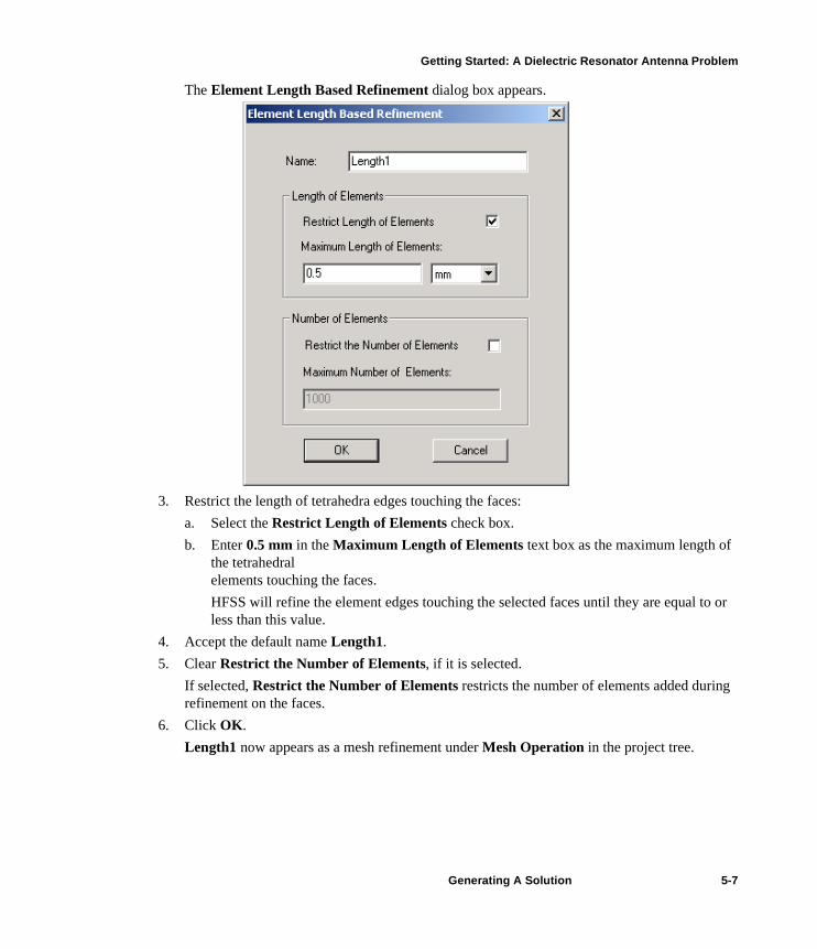
The Element Length Based Refinement dialog box appears.
3. Restrict the length of tetrahedra edges touching the faces:a. Select the Restrict Length of Elements check box.b. Enter 0.5 mm in the Maximum Length of Elements text box as the maximum length of
the tetrahedral �elements touching the faces.HFSS will refine the element edges touching the selected faces until they are equal to or less than this value.
4. Accept the default name Length1.5. Clear Restrict the Number of Elements, if it is selected.
If selected, Restrict the Number of Elements restricts the number of elements added during refinement on the faces.
6. Click OK. Length1 now appears as a mesh refinement under Mesh Operation in the project tree.
Generating A Solution 5-7

Getting Started: A Dielectric Resonator Antenna Problem
Validate the Project SetupBefore you run an analysis on the antenna model, it is important to first perform a validation check on the project. HFSS runs a check on all the setup details of the active project to verify that all the necessary steps have been completed and their parameters are reasonable. To perform a validation check on the project dra_antenna: 1. Click HFSS>Validation Check, or click the Validation Check button on the toolbar.
HFSS checks the project setup, and then the Validation Check window appears. 2. View the results of the validation check in the Validation Check window.
For this antenna project, a green check mark should appear next to each project step in the list. The following icons can appear next to an item:
3. If the validation check indicates that a step in your antenna project is incomplete or incorrect, go back to the step in HFSS and carefully review its setup along with its instructions as described in this manual.
4. Click Close. 5. Click File>Save to save any changes you may have made to your project.
�
Indicates the step is complete.
�
Indicates the step is incomplete.
�
Indicates the step may require your attention.
5-8 Generating A Solution

Getting Started: A Dielectric Resonator Antenna Problem
Generate the SolutionNow that you have entered all the appropriate solution criteria and defined the mesh operations, the antenna problem is ready to be solved. When you set up the solution criteria, you specified values for an adaptive analysis. An adaptive analysis is a solution process in which the mesh is refined iteratively in regions where the error is high, which increases the solution’s precision. You set the criteria that control mesh refinement dur-ing an adaptive field solution. Many problems can be solved using only adaptive refinement.The following is the general process carried out during an adaptive analysis:1. HFSS generates an initial mesh.2. Using the initial mesh, HFSS computes the electromagnetic fields that exist inside the structure
when it is excited at the solution frequency. (If you are running a frequency sweep, an adaptive solution is performed only at the specified solution frequency.)
3. Based on the current finite element solution, HFSS estimates the regions of the problem domain where the exact solution has strong error. Tetrahedra in these regions are refined.
4. HFSS generates another solution using the refined mesh. 5. The software recomputes the error, and the iterative process (solve — error analysis — refine)
repeats until the convergence criteria are satisfied or the requested number of adaptive passes is complete.
6. If a frequency sweep is being performed, HFSS then solves the problem at the other frequency points without further refining the mesh.
To begin the solution process:1. Select the Setup1 solution setup in the project tree.2. Click HFSS>Analyze. This command solves every solution setup in the design.
HFSS computes the 3D field solution inside the structure.The Progress window displays the solution progress as it occurs:
Note The results that you obtain should be approximately the same as the ones given in this section. However, there may be a slight variation between platforms.
Generating A Solution 5-9
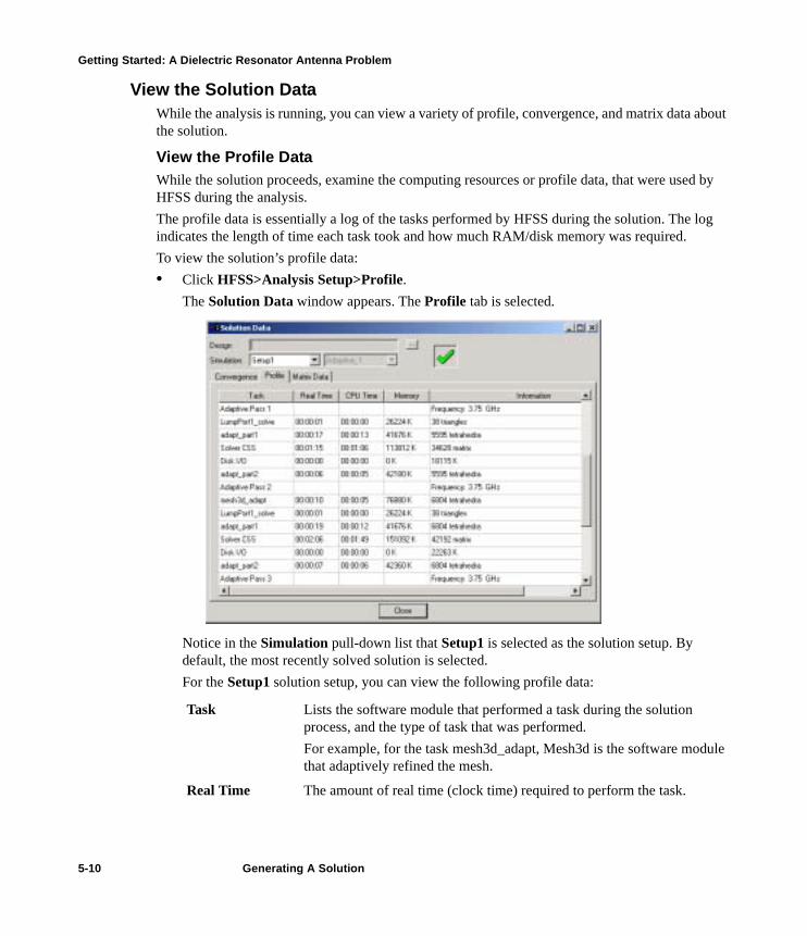
Getting Started: A Dielectric Resonator Antenna Problem
View the Solution DataWhile the analysis is running, you can view a variety of profile, convergence, and matrix data about the solution.
View the Profile DataWhile the solution proceeds, examine the computing resources or profile data, that were used by HFSS during the analysis. The profile data is essentially a log of the tasks performed by HFSS during the solution. The log indicates the length of time each task took and how much RAM/disk memory was required.To view the solution’s profile data:• Click HFSS>Analysis Setup>Profile.
The Solution Data window appears. The Profile tab is selected.
Notice in the Simulation pull-down list that Setup1 is selected as the solution setup. By default, the most recently solved solution is selected.For the Setup1 solution setup, you can view the following profile data:
Task Lists the software module that performed a task during the solution process, and the type of task that was performed. For example, for the task mesh3d_adapt, Mesh3d is the software module that adaptively refined the mesh.
Real Time The amount of real time (clock time) required to perform the task.
5-10 Generating A Solution
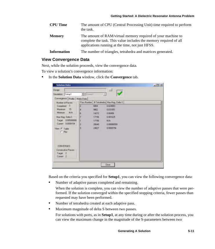
Getting Started: A Dielectric Resonator Antenna Problem
View Convergence DataNext, while the solution proceeds, view the convergence data. To view a solution’s convergence information:• In the Solution Data window, click the Convergence tab.
Based on the criteria you specified for Setup1, you can view the following convergence data:• Number of adaptive passes completed and remaining.
When the solution is complete, you can view the number of adaptive passes that were per-formed. If the solution converged within the specified stopping criteria, fewer passes than requested may have been performed.
• Number of tetrahedra created at each adaptive pass.• Maximum magnitude of delta S between two passes.
For solutions with ports, as in Setup1, at any time during or after the solution process, you can view the maximum change in the magnitude of the S-parameters between two �
CPU Time The amount of CPU (Central Processing Unit) time required to perform the task.
Memory The amount of RAM/virtual memory required of your machine to complete the task. This value includes the memory required of all applications running at the time, not just HFSS.
Information The number of triangles, tetrahedra and matrices generated.
Generating A Solution 5-11

Getting Started: A Dielectric Resonator Antenna Problem
consecutive passes. This information is available after two or more passes are completed.The convergence data can be displayed in table format or on a rectangular (X - Y) plot.
View Matrix DataNext, view matrices computed for the S-parameters, impedances, and propagation constants during each adaptive and sweep solution. To view matrices:1. In the Solution Data window, click the Matrix Data tab.
2. In the Simulation pull-down lists, do the following:a. Verify that Setup1 is selected as the solution setup for which you want to view matrices.b. Verify that LastAdaptive is selected. This is the solved pass for which you want to view
matrices. 3. Select S Matrix as the type of matrix data you want to view. 4. Select Magnitude/Phase from the pull-down list as the format in which to display the matrix
information.
5-12 Generating A Solution

Getting Started: A Dielectric Resonator Antenna Problem
You can display matrix data in the following formats:
5. Select the solved frequencies to display:• To display the matrix entries for all solved frequencies, select All Freqs. It is selected be
default.• To show the matrix entries for one solved frequency, clear All Freqs and then select the
solved frequency for which you want to view matrix entries. For adaptive passes, only the solution frequency specified in the Solution Setup dialog box is available. For frequency sweeps, the entire frequency range is available.The data is displayed in the table.6. Click Close to close this window.Once the simulation has run successfully, you will be ready to analyze the results, as described in the next chapter, “Analyzing the Solution.”
Magnitude/Phase Displays the magnitude and phase of the matrix type.
Real/Imaginary Displays the real and imaginary parts of the matrix type.
dB/Phase Displays the magnitude in decibels and phase of the matrix type.
Phase Displays the phase of the matrix type.
Real Displays the real parts of the matrix type.
Magnitude Displays the magnitude of the matrix type.
Imaginary Displays the imaginary parts of the matrix type.
dB Displays the magnitude in decibels of the matrix type.
Generating A Solution 5-13

Getting Started: A Dielectric Resonator Antenna Problem
5-14 Generating A Solution

Analyzing the Solution
Now, HFSS has generated a solution for the antenna problem. In general, you can display and �analyze the results of a project in many different ways. You can:• Plot field overlays - representations of basic or derived field quantities - on surfaces or objects. • Create 2D or 3D rectangular or circular plots and data tables of S-parameters, basic and
derived field quantities, and radiated field data.• Plot the finite element mesh on surfaces or within 3D objects.• Create animations of field quantities, the finite element mesh, and defined project variables.• Scale an excitation’s magnitude and modify its phase.• Delete solution data that you do not want to store.For this antenna problem, you will specifically: • Create Modal S-parameter reports. • Create a field overlay plot of the magnitude of E on the top face of the antenna’s cavity.• Create an animation of the mag-E plot.
Time It should take you approximately 1 hour to work through this chapter.
Analyzing the Solution 6-1
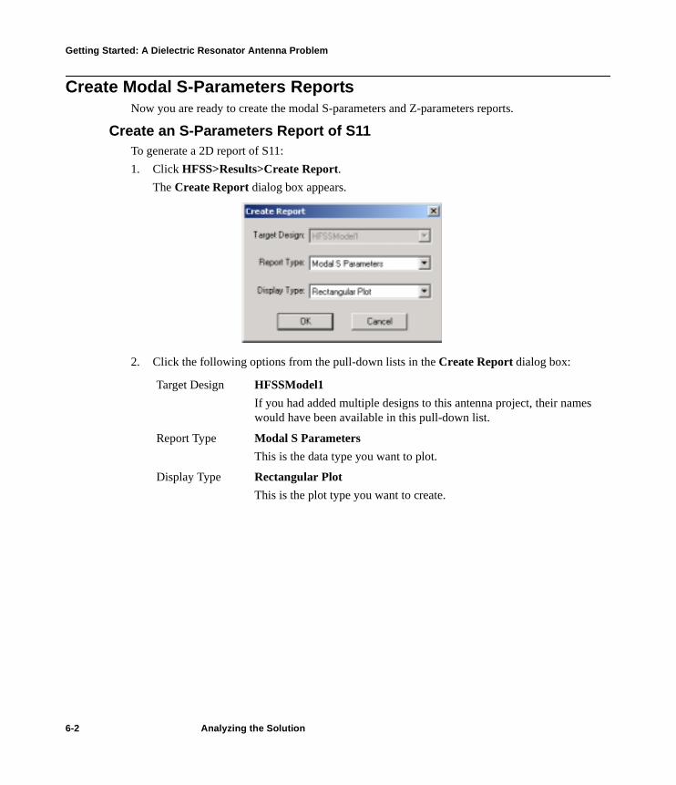
Getting Started: A Dielectric Resonator Antenna Problem
Create Modal S-Parameters ReportsNow you are ready to create the modal S-parameters and Z-parameters reports.
Create an S-Parameters Report of S11To generate a 2D report of S11:1. Click HFSS>Results>Create Report.
The Create Report dialog box appears.
2. Click the following options from the pull-down lists in the Create Report dialog box:
Target Design HFSSModel1If you had added multiple designs to this antenna project, their names would have been available in this pull-down list.
Report Type Modal S ParametersThis is the data type you want to plot.
Display Type Rectangular PlotThis is the plot type you want to create.
6-2 Analyzing the Solution
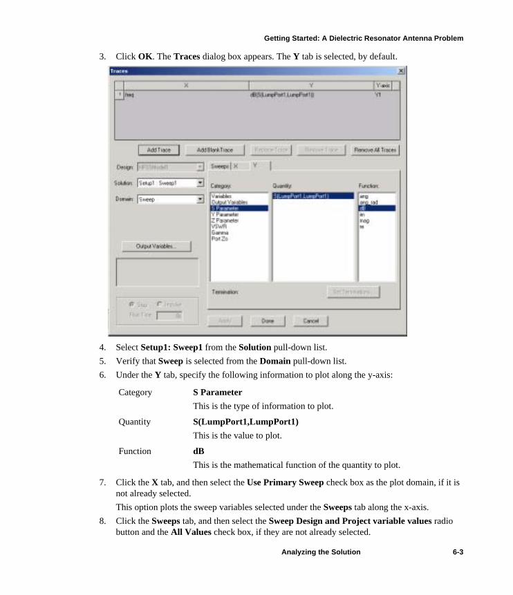
Getting Started: A Dielectric Resonator Antenna Problem
3. Click OK. The Traces dialog box appears. The Y tab is selected, by default.
4. Select Setup1: Sweep1 from the Solution pull-down list. 5. Verify that Sweep is selected from the Domain pull-down list.6. Under the Y tab, specify the following information to plot along the y-axis:
7. Click the X tab, and then select the Use Primary Sweep check box as the plot domain, if it is not already selected. This option plots the sweep variables selected under the Sweeps tab along the x-axis.
8. Click the Sweeps tab, and then select the Sweep Design and Project variable values radio button and the All Values check box, if they are not already selected.
Category S ParameterThis is the type of information to plot.
Quantity S(LumpPort1,LumpPort1)This is the value to plot.
Function dBThis is the mathematical function of the quantity to plot.
Analyzing the Solution 6-3
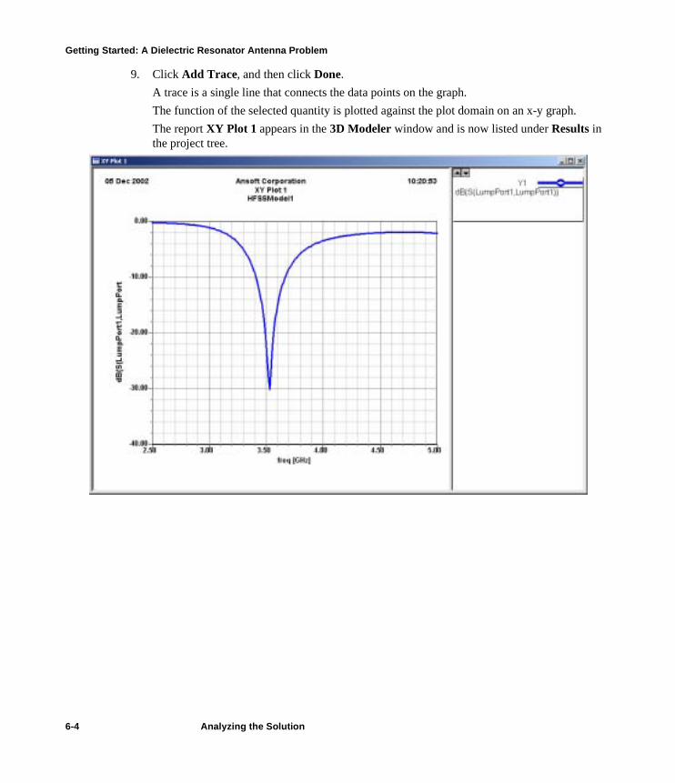
Getting Started: A Dielectric Resonator Antenna Problem
9. Click Add Trace, and then click Done. A trace is a single line that connects the data points on the graph.The function of the selected quantity is plotted against the plot domain on an x-y graph. The report XY Plot 1 appears in the 3D Modeler window and is now listed under Results in the project tree.
6-4 Analyzing the Solution

Getting Started: A Dielectric Resonator Antenna Problem
Create an S-Parameters Report of Z11To generate a 2D report of Z11 Real and Imaginary traces:1. Click HFSS>Results>Create Report.
The Create Report dialog box appears.2. Click the following options from the pull-down lists in the Create Report dialog box:
3. Click OK. The Reporter dialog box appears. The Y tab is selected, by default.
Target Design HFSSModel1
Report Type Modal S Parameters
Display Type Rectangular Plot
Analyzing the Solution 6-5
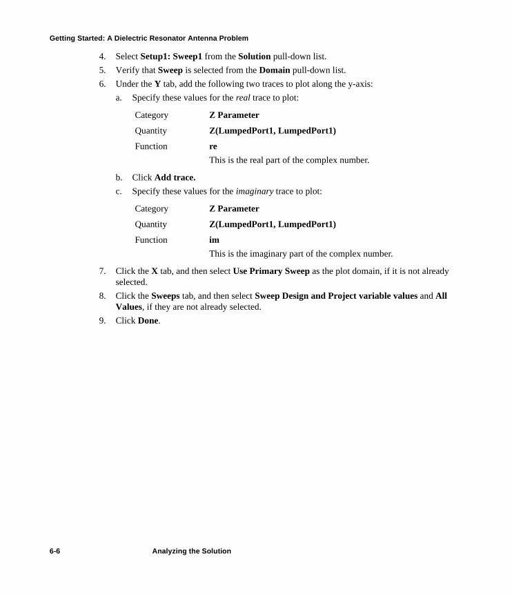
Getting Started: A Dielectric Resonator Antenna Problem
4. Select Setup1: Sweep1 from the Solution pull-down list. 5. Verify that Sweep is selected from the Domain pull-down list.6. Under the Y tab, add the following two traces to plot along the y-axis:
a. Specify these values for the real trace to plot:
b. Click Add trace.c. Specify these values for the imaginary trace to plot:
7. Click the X tab, and then select Use Primary Sweep as the plot domain, if it is not already selected.
8. Click the Sweeps tab, and then select Sweep Design and Project variable values and All Values, if they are not already selected.
9. Click Done.
Category Z Parameter
Quantity Z(LumpedPort1, LumpedPort1)
Function reThis is the real part of the complex number.
Category Z Parameter
Quantity Z(LumpedPort1, LumpedPort1)
Function imThis is the imaginary part of the complex number.
6-6 Analyzing the Solution

Getting Started: A Dielectric Resonator Antenna Problem
The report XY Plot 2 appears in the 3D Modeler window and is now listed under Results in the project tree.
Analyzing the Solution 6-7

Getting Started: A Dielectric Resonator Antenna Problem
Create Field Overlay PlotsNext, you will create a field overlay plot of the magnitude of E of the bottom face of the antenna’s �air volume object and examine the resulting E- field pattern.
Create a Mag E Field Overlay PlotNow, you are ready to create a field overlay plot of the magnitude of E of the bottom face of the air volume object and examine the resulting E- field pattern. 1. In Select Faces mode, click the bottom face of the object airvol. 2. On the HFSS menu, point to Fields>Plot Fields, and then click Mag_E.
The Create Field Plot dialog box appears.
3. Select Mag_E from the Quantity list. This selects the magnitude of the real part of the electric field |E|(x,y,z,t) as the quantity to plot.
4. Select All from the In Volume list to specify that HFSS will plot over the entire volume of the model.
5. Verify that 3.75GHz is selected from the Freq pull-down list. The Freq pull-down list includes a list of frequencies for which a field solution is available.
6. Verify that 0deg is selected from the Phase pull-down list.7. Click Done.
6-8 Analyzing the Solution
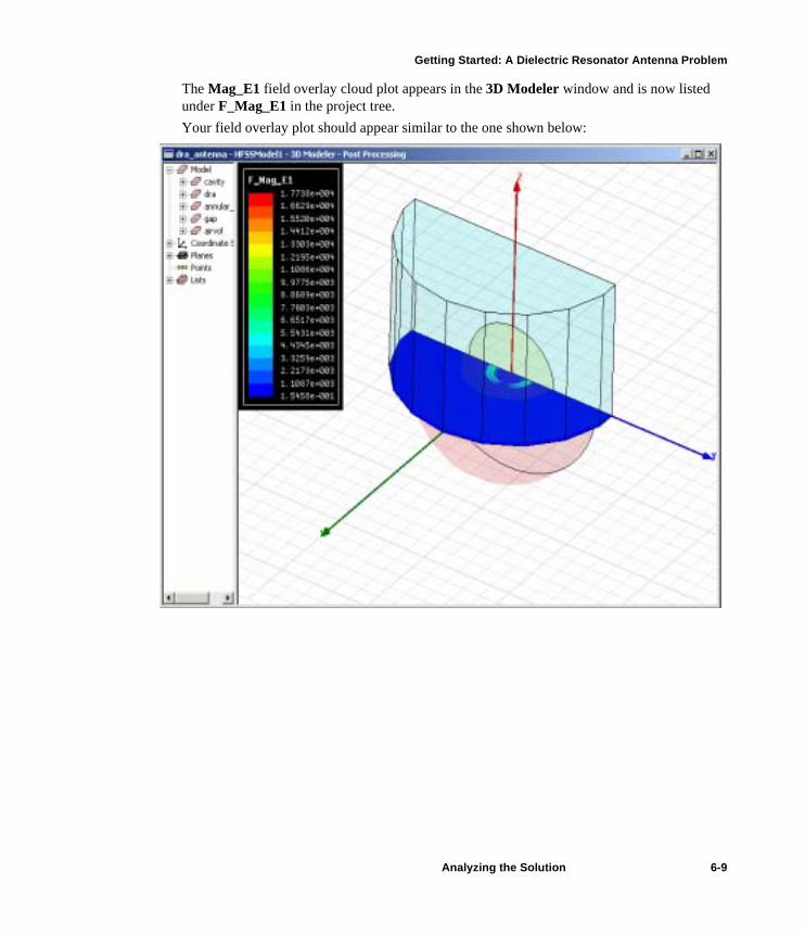
Getting Started: A Dielectric Resonator Antenna Problem
The Mag_E1 field overlay cloud plot appears in the 3D Modeler window and is now listed under F_Mag_E1 in the project tree. Your field overlay plot should appear similar to the one shown below:
Analyzing the Solution 6-9
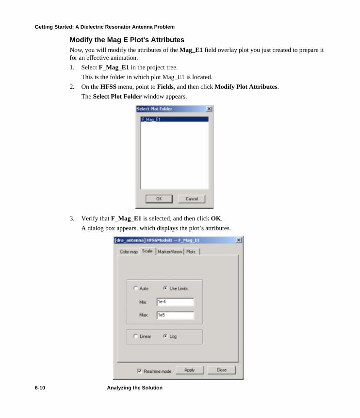
Getting Started: A Dielectric Resonator Antenna Problem
Modify the Mag E Plot’s AttributesNow, you will modify the attributes of the Mag_E1 field overlay plot you just created to prepare it for an effective animation. 1. Select F_Mag_E1 in the project tree.
This is the folder in which plot Mag_E1 is located. 2. On the HFSS menu, point to Fields, and then click Modify Plot Attributes.
The Select Plot Folder window appears.
3. Verify that F_Mag_E1 is selected, and then click OK. A dialog box appears, which displays the plot’s attributes.
6-10 Analyzing the Solution
Getting Started: A Dielectric Resonator Antenna Problem
4. Click the Color map tab, and then specify the following settings:
5. Click the Scale tab, and then specify the following settings:
6. Click the Plots tab, and then specify the following settings:
7. Accept all the remaining default settings in this dialog box, and then click Apply.
Type Select Spectrum and Rainbow from the pull-down list. Field quantities are plotted in multiple colors. Each field value is assigned a color from the selected spectrum.
Number of colors Enter 32. This is the number of colors that will be used in the plot.
Real time mode Select this option.This option immediately applies changes to the plot’s attributes.
Use Limits Select this option.Only the field values between the minimum and maximum values will be plotted. Field values below or above these values will be plotted in the colors assigned to the minimum or maximum limits, respectively.
Min Enter 1e-4 (0.0001).
Max Enter 1e5 (100000).
Linear/ Log Select Log. Field values will be plotted on a logarithmic scale.
IsoValType Select Tone from the pull-down list. This isosurface display type varies color continuously between isovalues.
Outline Select this option.
Map transp. Clear this option, if it is selected. If selected, the transparency of field values increases as the solution values decrease.
Smooth shade Select this option.
Analyzing the Solution 6-11
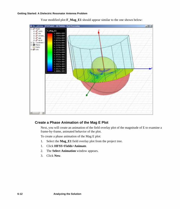
Getting Started: A Dielectric Resonator Antenna Problem
Your modified plot F_Mag_E1 should appear similar to the one shown below:
Create a Phase Animation of the Mag E PlotNext, you will create an animation of the field overlay plot of the magnitude of E to examine a frame-by-frame, animated behavior of the plot. To create a phase animation of the Mag E plot: 1. Select the Mag_E1 field overlay plot from the project tree.1. Click HFSS>Fields>Animate.2. The Select Animation window appears. 3. Click New.
6-12 Analyzing the Solution

Getting Started: A Dielectric Resonator Antenna Problem
The Setup Animation dialog box appears.
4. Accept the default name Animation1 in the Name text box.5. Optionally, type a description of the animation in the Description text box.6. Under the Swept Variable tab, select Phase from the Swept Variable list.7. Accept the remaining default settings in the Start, Stop, and Steps boxes for the phase �
values of the animation. If the Start value is 10, the Stop value is 160, and the number of steps is 10, the animation will display the plot at 10 phase values between 10 and 160. The start value will be the first frame displayed, resulting in a total of 11 frames in the animation.
8. Click OK.The animation begins in the 3D Modeler window. The play panel appears in the upper-left corner of the desktop, enabling you to stop, restart, and control the speed and sequence of the frames.
Analyzing the Solution 6-13

Getting Started: A Dielectric Resonator Antenna Problem
6-14 Analyzing the Solution

Index
Numerics3D Modeler window
defined 2-3location on desktop 2-2overview 3-3
Aadaptive solution 5-2air volume 3-21
assigning a color to 3-22assigning a transparency to 3-22assigning perfect E boundary to 4-4assigning radiation boundary to 4-3naming 3-22verifying its material 3-22
analysisof solution 6-1results 1-3
animationcreating a phase animation 6-12
annular feed ring 3-14assigning a color to 3-17assigning a transparency to 3-17assigning perfect H boundary to 4-7naming 3-17
automatically set min/max triangles 5-4
Bboundaries
about 4-2assigning 4-3assigning a perfect E boundary 4-4assigning a perfect H boundary 4-7assigning a radiation boundary 4-3assigning a symmetry boundary 4-8editing visualization settings of 4-3model-specific conditions 4-2solver view of 4-13verifying 4-13
Ccavity
assigning a color to 3-7assigning a transparency to 3-8naming 3-6splitting 3-6verifying its material 3-8
clone before intersect 3-19context-sensitive help 2-5coordinate system
about 3-4
Index-1
face type 3-4global type 3-4relative type 3-4
Ddesign, inserting 2-4dialog boxes
Create Field Plot 6-8Create Report 6-2, 6-5Edit Sweep 5-5Element Length based refinement 5-7Lumped Port wizard 4-10Port Impedance Multiplier 4-12Reporter 6-5Set Model Units 3-4Setup Animation 6-13Solution Setup 5-2Solution Type 3-2Split 3-6Symmetry Boundary 4-9Traces 6-3View/Edit Material 3-13
Do lambda refinement option 5-3DRA 3-9
assigning a color to 3-11assigning a material to 3-12assigning a transparency to 3-11naming 3-10splitting 3-10
drawingcircles 3-14polyhedrons 3-21rectangles 3-18setting the drawing units 3-4spheres 3-5, 3-9the air volume object 3-21the annular feed ring object 3-14the DRA object 3-9the feed gap object 3-18
drawing region 3-3
EE-field
analyzing 6-8animating 6-12plotting 6-8
excitationsabout 4-2assigning 4-10impedance multiplier 4-12model-specific conditions 4-2solver view of 4-13verifying 4-13
FF1 key 2-5feed gap 3-18
assigning a color to 3-20assigning a transparency to 3-20assigning lumped port to 4-10naming 3-20
field overlay plotscreating 6-8modifying attributes of 6-10
frequency sweepadding 5-5defining the sweep 5-5saving fields 5-6
Ggeometric model
assigning symmetry boundary to 4-8fitting in drawing region 3-5sample problem 1-2solution parameters 5-2splitting for symmetry 3-23
graphical user interface 2-2grid
setting its drawing units 3-4
Index-2

Hhelp
accessing 2-5context-sensitive 2-5
HFSSfile extensions 2-5inserting an HFSS design 2-4interface overview 2-2
history treedefined 2-3location on desktop 2-2
Iimpedance multiplier
about 4-12modifying 4-12
infinite ground plane 4-6installation 2-1integration line, defining 4-10
Llighting
ambient 3-8disable attributes 3-8distant 3-8
lumped port 4-2lumped ports
and defining the integration line 4-10assigning 4-10editing 4-11impedance multiplier 4-12
Mmag E
field overlay plots of 6-8Mag E, plotting 6-8manual
printing history 1-iiitypeface conventions 1-iv
materials
assigning 3-12creating new 3-12verifying 3-8, 3-22
menu bardefined 2-3location on desktop 2-2
meshdefining mesh operations 5-6refining 5-6seeding 5-6
mesh operations 5-6restricting length 5-7
Message Manager windowdefined 2-3location on desktop 2-2
Oobjects
air volume 3-21annular feed ring 3-14assigning color to 3-7, 3-11, 3-17, 3-20, 3-22assigning lumped ports to 4-10assigning materials to 3-12assigning transparency to 3-8, 3-11, 3-17, 3-
20, 3-22DRA 3-9feed gap 3-18intersecting 3-19naming 3-6, 3-10, 3-17, 3-20, 3-22selecting faces of 4-5sheet object defined 3-17splitting 3-6, 3-10splitting for symmetry 3-23subtracting 3-15
Pperfect E boundary
assigning 4-4defined 4-2
perfect H boundaryassigning 4-7defined 4-2
Index-3
plotsanimating 6-12appearance in the project tree 6-4, 6-7creating a cloud plot 6-8creating a mag E plot 6-8creating field overlays 6-8modifying attributes of 6-10
port impedanceimaginary 4-10real 4-10
profile data 5-10Progress window
defined 2-3displaying solution progress 5-9location on desktop 2-2
projectvalidating 5-8
Project Manager windowdefined 2-3location on desktop 2-2
project treeinserting an HFSS design 2-4
projectsadding 2-4adding project notes 2-5creating 2-4saving 2-5
Properties windowdefined 2-3location on desktop 2-2
Rradiation boundary
assigning 4-3defined 4-2
reportsadding traces 6-4animating 6-12appearance in the project tree 6-4, 6-7creating a cloud plot 6-8creating S11 6-2creating Z11 6-5field overlay plots 6-8
generating 2D graphs 6-2modal S-parameters 6-2
rescale to new units 3-4
SS11
creating report of 6-2select faces mode 4-5setting up 3-3simulation
running 5-9solution
adding a fast frequency sweep 5-5adding to a design 5-2analyzing 6-1automatically set min/max triangles 5-4defining mesh operations 5-6generating 5-9specifying frequency 5-3specifying lambda refinement 5-3specifying maximum delta S 5-3specifying maximum number of passes 5-3specifying minimum converged passes 5-4viewing convergence data 5-11viewing matrix data 5-12viewing profile data 5-10
solution typesDriven Modal 3-2Driven Terminal 3-2Eigenmode 3-2selecting 3-2
solutionsadaptive 5-2adaptive analysis 5-9adding a solution setup 5-2and setting parameters 5-2frequency 5-2setting solution parameters 5-2
status bardefined 2-3location on desktop 2-2
subtractingand blank objects 3-15
Index-4

and tool objects 3-15symmetry boundary
assigning 4-8defined 4-2
Ttoolbars
defined 2-3location on desktop 2-2
trace, adding 6-4
Uunits, selecting 3-4
Vvalidation check 5-8
Wwave ports
impedance multiplier 4-12
ZZ11
creating report of 6-5
Index-5

Index-6


![ANTENNA BEHAVIOUR UNDER DIFFERENT SOIL CONDITIONS...[21] Varun Shukla, Arti Saxena and Swati Jain, A New Rectangular Dielectric Resonator Antenna Compatible for Mobile Communication](https://img.pdfslide.us/doc/110x75/5f935e7cb3469a48e978d7c8/antenna-behaviour-under-different-soil-21-varun-shukla-arti-saxena-and-swati.jpg)