Getting rid of stochasticity

(applicable sometimes)

Han HoogeveenUniversiteit Utrecht

Joint work with Marjan van den Akker

Outline of the talk

• Problem description• How to solve the deterministic problem• Stochastic processing times

– consequences– four classes of instances

• Stochastic machine• Processing times and machine

stochastic

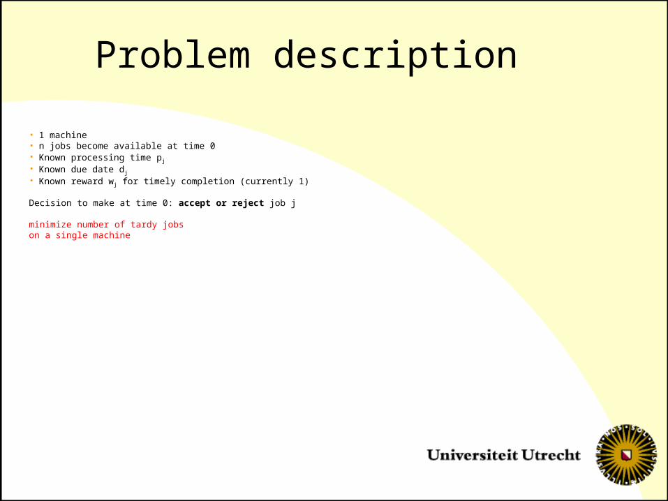
Problem description

• 1 machine• n jobs become available at time 0• Known processing time pj

• Known due date dj

• Known reward wj for timely completion (currently 1)

Decision to make at time 0: accept or reject job j

minimize number of tardy jobs on a single machine

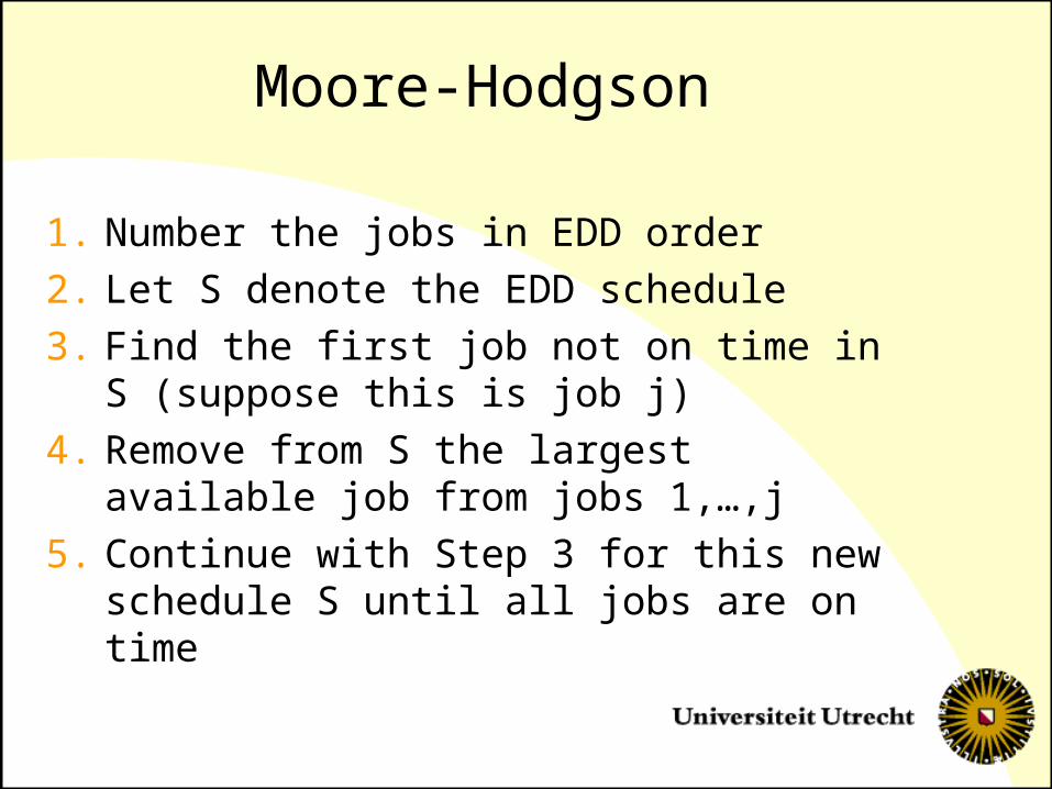
Moore-Hodgson

1. Number the jobs in EDD order2. Let S denote the EDD schedule3. Find the first job not on time in S

(suppose this is job j)4. Remove from S the largest available

job from jobs 1,…,j5. Continue with Step 3 for this new

schedule S until all jobs are on time

Solving the problem from scratch

Observations• First the on time jobs• On time jobs in EDD order• Forget about the late jobs (once rejected

= lost for ever)

Knowing the on time set is sufficient

Dominance rule

• Let E1 and E2 be two subsets of jobs 1,…,j• All jobs in E1 and E2 are on time (feasible)• Cardinality of E1 and E2 is equal• The total processing time of the jobs in E2

is more than the total processing time of the jobs in E1

Then subset E2 can be discarded.

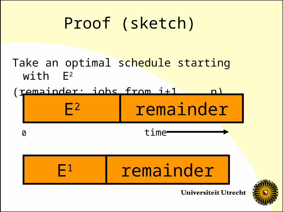
Proof (sketch)

Take an optimal schedule starting with E2

(remainder: jobs from j+1, …, n)

E2 remainder

E1 remainder

time0

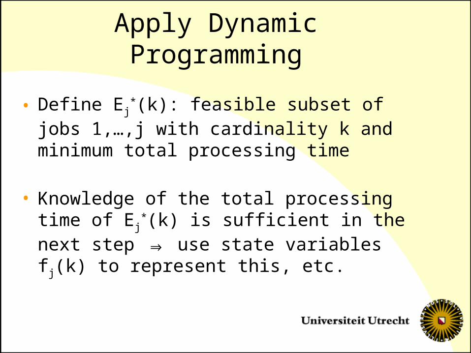
Apply Dynamic Programming

• Define Ej*(k): feasible subset of jobs 1,

…,j with cardinality k and minimum total processing time

• Knowledge of the total processing time of Ej

*(k) is sufficient in the next step ⇒ use state variables fj(k) to represent this, etc.

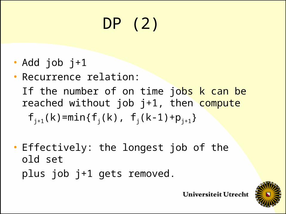
DP (2)

• Add job j+1• Recurrence relation:

If the number of on time jobs k can be reached without job j+1, then compute fj+1(k)=min{fj(k), fj(k-1)+pj+1}

• Effectively: the longest job of the old setplus job j+1 gets removed.

Further remarks

• DP computes more state variables than necessary

• DP can be used for the weighted case:– Use fj(W) with W is the total weight of the on

time set (instead of cardinality of the on time set)

• DP can be used for more problems

Stochastic processing times

• Completion times are uncertain

• Decision about accept or reject must be made before running the schedule

• When do you consider a job on time?

On time stochastically

• Work with a sequence of on time jobs (instead of a set of completion times)

• Add a job to this sequence and compute the probability that it is ready on time

• If this probability is large enough (at least equal to the minimum success probability msp) then accept it as on time

Classes of processing times

• Gamma distribution• Negative binomial distribution

• Equally disturbed processing times pj

• Normal distribution

Jobs must be independent

Class 1: Gamma distribution

• Parameters aj and b (common)

• If X1 and X2 follow the gamma distribution and are independent, then X1+X2 is gamma distributed with parameters a1+a2 and b (we call this additive).

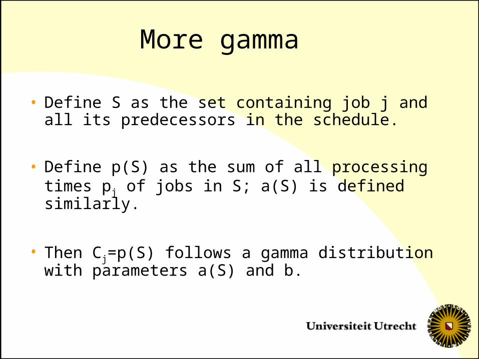
More gamma

• Define S as the set containing job j and all its predecessors in the schedule.

• Define p(S) as the sum of all processing times pj of jobs in S; a(S) is defined similarly.

• Then Cj=p(S) follows a gamma distribution with parameters a(S) and b.

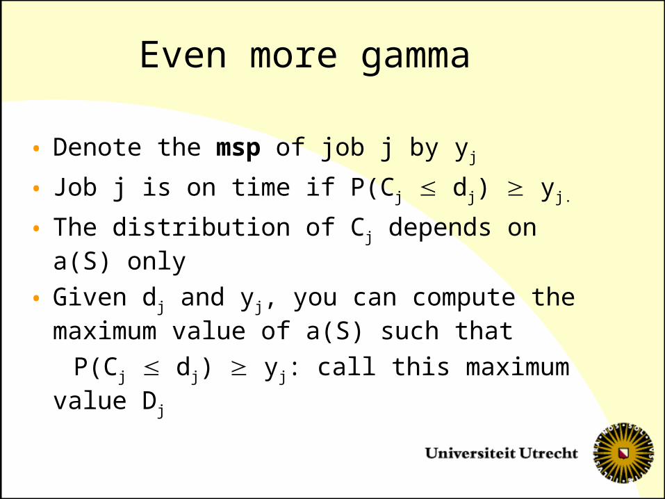
Even more gamma

• Denote the msp of job j by yj

• Job j is on time if P(Cj dj) yj.

• The distribution of Cj depends on a(S) only

• Given dj and yj, you can compute the maximum value of a(S) such that

P(Cj dj) yj: call this maximum value Dj

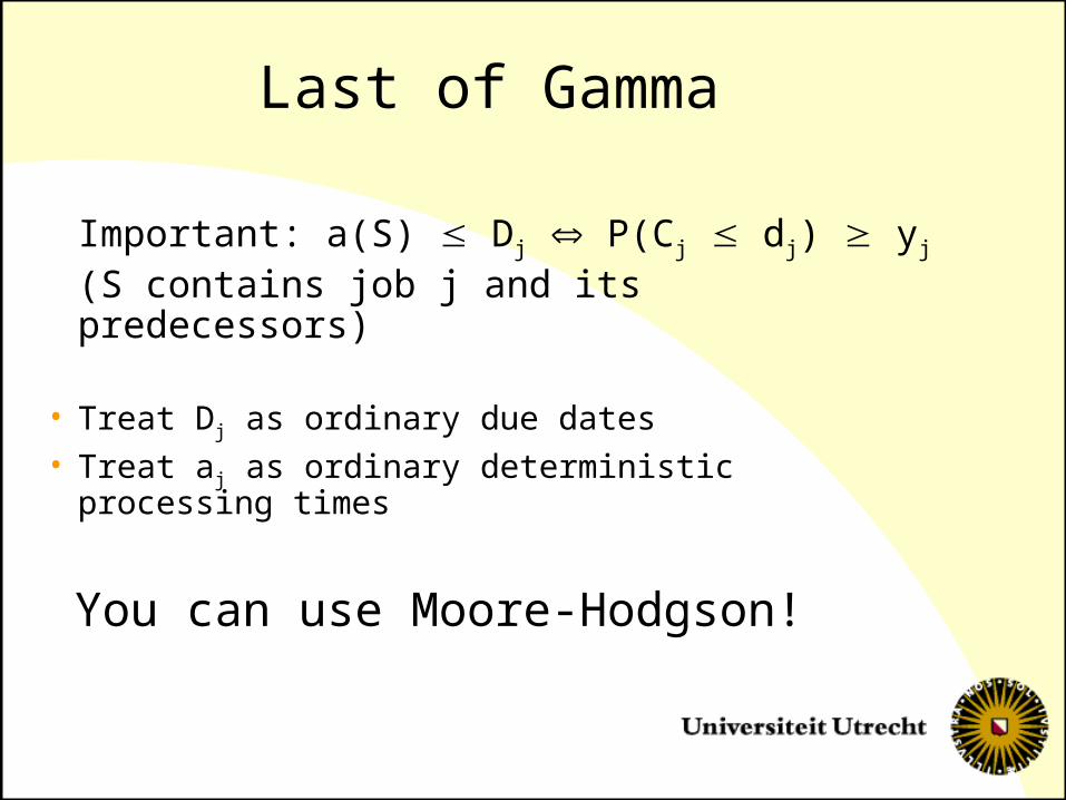
Last of Gamma

Important: a(S) Dj P(Cj dj) yj

(S contains job j and its predecessors)

• Treat Dj as ordinary due dates• Treat aj as ordinary deterministic processing

times

You can use Moore-Hodgson!

Negative binomial distribution

• Parameters s_j and p (common for all jobs)

• If independent, then C_j=p(S) follows a negative binomial distribution with parameters s(S) and p

Solvable like the gamma distribution

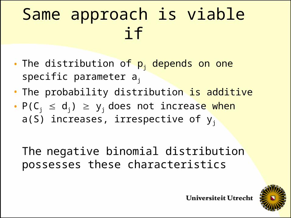
Same approach is viable if

• The distribution of pj depends on one specific parameter aj

• The probability distribution is additive

• P(Cj dj) yj does not increase when a(S) increases, irrespective of yj

The negative binomial distribution possesses these characteristics

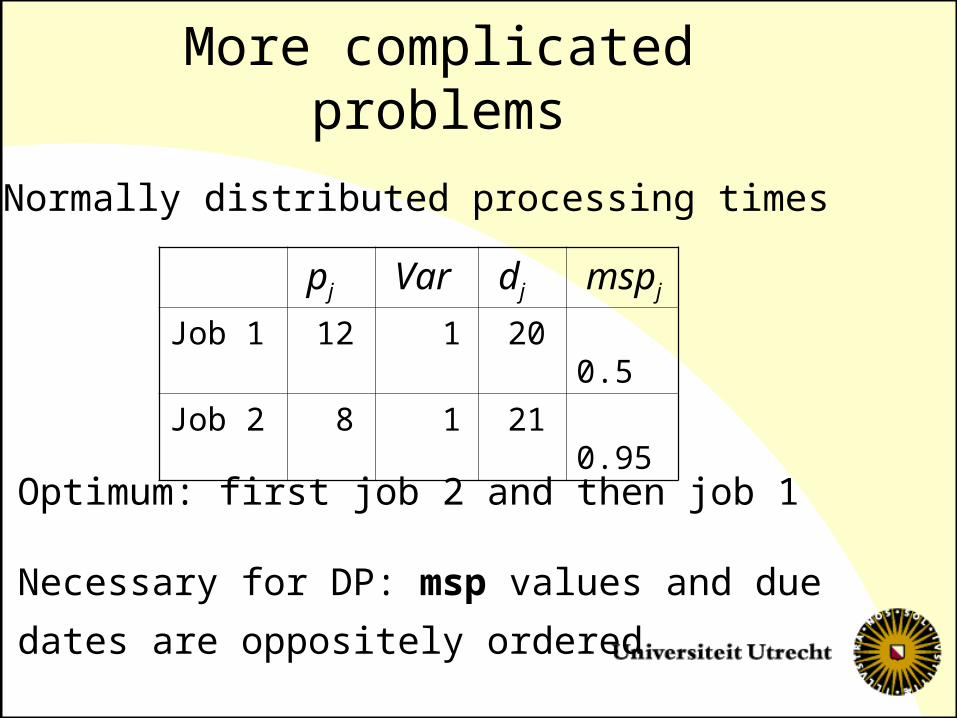
More complicated problems

pj Var dj mspj

Job 1 12 1 20 0.5

Job 2 8 1 21 0.95

Normally distributed processing times

Optimum: first job 2 and then job 1

Necessary for DP: msp values and due

dates are oppositely ordered

Equal disturbances• On time probability of job j depends on:

– Number of predecessors (on time jobs before j)– Total processing time of its predecessors

• Dominance rule: given the cardinality of the on time set, take the one with minimum total processing time

• Use dynamic programming with state variables fj(k) that indicate the minimum total processing time possible (as before)

• Hence: Moore-Hodgson’s solves it!

Normal distribution (1)

• Parameters: expected processing time of job j and variance of job j

• Two parameters ⇒ simple approach fails

• Reminder: expected value and variances of X1+X2 are equal to the respective sums

• Necessary for computing the on time probability of job j:– Total processing time of predecessors– Total variance of predecessors

Normal distribution (2)

• Dominance rule: if cardinality and total processing time are equal, then take the set with minimum total variance (msp > 0.5)

• Use state variables fj(k,P):– k is cardinality of on time set– P is total processing time of on time set

– fj(k,P) is minimum variance possible

Normal distribution: details

• Running time pseudo-polynomial

• Problem is NP-hard

• Role of total variance and total processing time in the dominance rule and in the DP is interchangeable

Unreliable machine

• Assume deterministic processing times• Amount of work done by the machine

per period is stochastic• Define X(t) as the stochastic variable

denoting the amount of work done in [0,t]

• Assume that the probability distribution of X(t) is known

Solution method

• Use the minimum success probability yj

• Again, use S to denote job j and its predecessors in the schedule; the total processing time of S is p(S)

• Job j is stochastically on time if P(X(dj) p(S)) yj

Solution method (2)

• Compute Dj as the maximum value of p(S) such that P(X(dj) p(S)) yj .

• Treat the Dj values as the traditional due dates for a reliable machine.

=> Traditional deterministic problem

Moore-Hodgson solves it

Everything unreliable

• Same approach as with the unreliable machine:– X(t) denotes the amount of work done in

[0,t]– p(S) is total processing time of the jobs in S;

this is a stochastic variable now– Job j is stochastically on time if P(X(dj) p(S)) yj

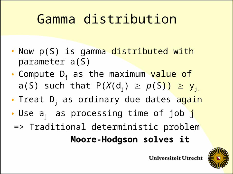
Gamma distribution

• Now p(S) is gamma distributed with parameter a(S)

• Compute Dj as the maximum value of a(S) such that P(X(dj) p(S)) yj.

• Treat Dj as ordinary due dates again

• Use aj as processing time of job j

=> Traditional deterministic problem Moore-Hodgson solves it

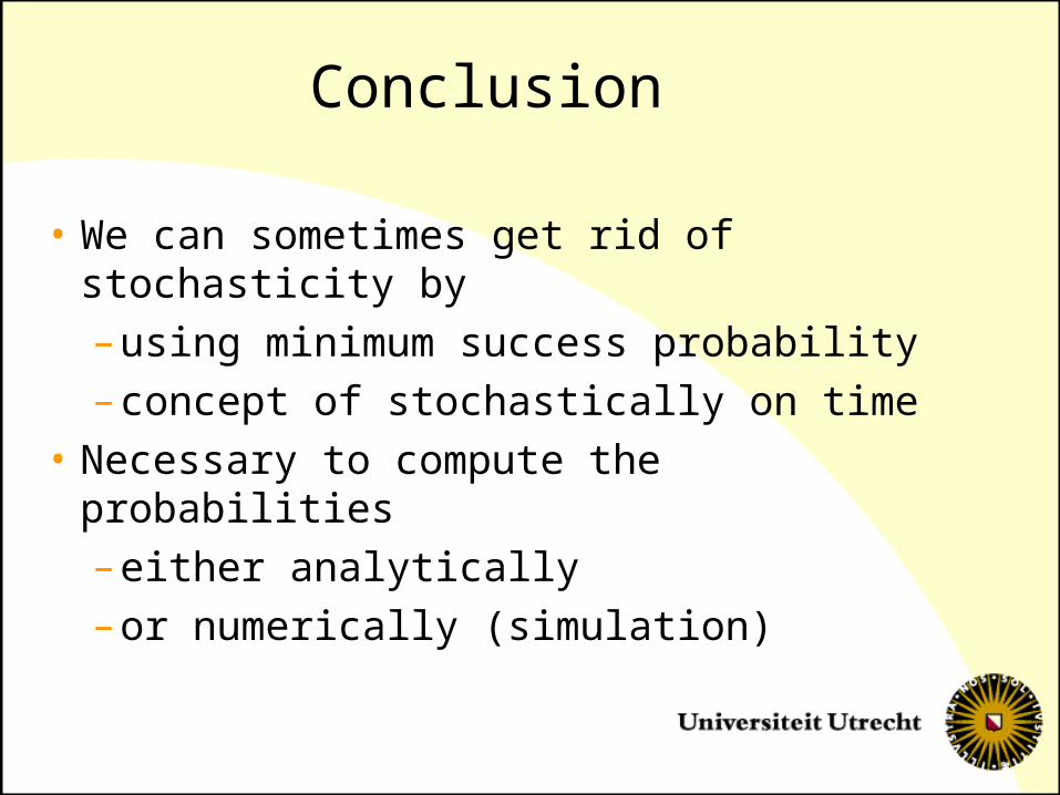
Conclusion

• We can sometimes get rid of stochasticity by – using minimum success probability– concept of stochastically on time

• Necessary to compute the probabilities– either analytically– or numerically (simulation)

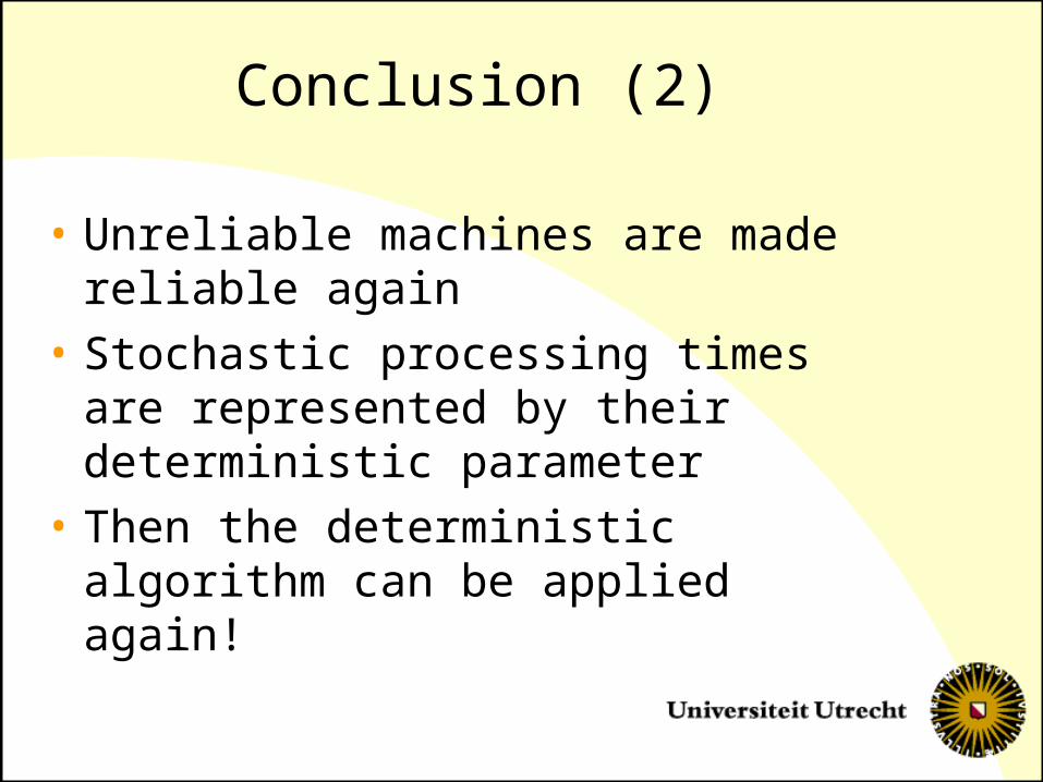
Conclusion (2)

• Unreliable machines are made reliable again

• Stochastic processing times are represented by their deterministic parameter

• Then the deterministic algorithm can be applied again!