Get the Best Out Of SAS ODS Graphics and the SG … · 1 Paper DV13-2012 . Get the Best Out Of SAS® ODS Graphics and the SG (Statistical Graphics) Procedures: Communication-Effective

1

Paper DV13-2012

Get the Best Out Of SAS® ODS Graphics and the SG (Statistical Graphics) Procedures: Communication-Effective Charts, Things That SAS/GRAPH® Cannot Do As Well,

and Macro Tools To Save Time and Avoid Errors

LeRoy Bessler PhD, Bessler Consulting and Research, [email protected] ABSTRACT ODS Graphics and the SG (Statistical Graphics) Procedures are now built into Version 9.3 of Base SAS, and entail no additional software licensing charge. However, this technology comes with options and features that require optimization by you to actually get communication-effective output if you want more than simply the default results that come with no added thought or effort. This paper prescribes principles of communication-effective graphic design, and shows you how to implement them. For certain charts, macros are provided to make getting desired results easy and quick. Less code means less opportunity for coding error. The paper also emphasizes and delivers widely usable solutions that were impossible or less well rendered with SAS/GRAPH. The new tools manifest some unexpected behaviors, which do not even announce themselves in the SAS log. The paper points these out, and shows how to cope with them. After thirty years of working to get the best out of SAS/GRAPH, and twenty-five years of sharing my SAS/GRAPH solutions with SAS users, I have become a convert to the new technology. Come learn how to get the best from it. INTRODUCTION This tutorial shows you easy ways to get beyond taking the defaults, to get better results with minimum time and effort. It covers pie, bar, and line charts written to disk to later be inserted into Microsoft PowerPoint, Word, or Excel, or simply printed, but also emphasizes and demonstrates the benefits of web-enabled time series plots, and shows how to create them. For pie charts and bar charts it has long been possible to display the associated precise numbers as part of the image, but for graphs with plot points on multiple lines and/or with point-dense single lines, it has not. For time series or line charts, the paper demonstrates three ways to address this: (1) ALT text (a.k.a. “data tips”, mouseover text, flyover text, hover text, floatover text, tool tips, or pop-up text—which is my name for it); (2) a companion spreadsheet linked to the plot; and (3) a table imbedded in the plot image. The first two options can be used only with web-enabled plots. The third option is available for static plots that are printed or deployed in slides or electronic documents, and for web-enabled plots, and is easier to do with ODS GRAPHICS than with SAS/GRAPH. My focus is on graphs used for management reporting in business, government, or other organizational settings, not statistical or heavy-duty analytical graphs. Although the SG (Statistical Graphics) procedures were originally developed for statistical graphics, they can be used for management reporting. By graphs for management reporting I mean graphs or web graphs used to answer several common questions. How are things going? Are they better, worse, or about the same? How do measurements for different entities compare? Questions like these are commonly answered visually with time plots (or time series graphs), bar charts, and pie charts. For dramatic and unequivocal proof of the importance of graphing your data, see Reference 1. For some coding examples, macro-based solutions are also provided to make it easier and safe to create the results. UNEXPECTED THINGS ODS GRAPHICS DOES WITHOUT ANY WARNING MESSAGES 1. It can omit tick mark values that are essential (categorical character values, not values of a continuous numeric

variable) or in cases where you have explicitly specified the numeric or date values to be listed. This astonishing (and frustrating) feature is described in great detail in the paper, and circumvention options are covered.

2. It creates line breaks in your titles and footnotes when font size is too large for amount of text to fit on one line.

WISH FOR ODS GRAPHICS—the ability to force DESIRED line breaks with coding so that specification of text characteristics (font, size, color, etc.) does not have to be repeated in every TITLE statement. ALSO MISSING IN ODS GRAPHICS—the ability to specify default characteristics for all text in graph for which characteristics are not explicitly specified in code. Using GTL to create a custom style is extra and complex work.

2

PRINCIPLES OF COMMUNICATION-EFFECTIVE GRAPHICS I have recently been using Principia Graphika as a title for concise handouts on the Principles of Communication-Effective Graphics. They are some of the ideas and techniques that I have been implementing, advocating, and writing/speaking about for more than two decades. So, what are the Principles? Well, there are a lot of them, previously reported by me elsewhere. In this paper, the focus is on these: • Deliver image plus precise numbers: image for quick easy inference, precise numbers for reliable inference

• Provide ordering—Show them what’s important

• Subset the content where appropriate—Show them what’s important

• Provide a reliably usable legend—Seems like something that a user should be able to take for granted as built-in

• Suppress and avoid graphic frills—Let your data talk

3

Communication-Effective Graphic Design Principle 1: Deliver image plus precise numbers Graphs accelerate and facilitate inference and decision-making, but the actual numbers are required for reliable inference and decisions. My scope does include static graphs, i.e., ones destined directly for print (less frequent these days) or for imbedding in PowerPoint for presentations, in PDF for Adobe Acrobat Reader, or in RTF for Microsoft Word. However, web-enabled graphs are my preferred choice now, whenever the acceptable information delivery method. Web enablement provides quick and easy navigation between graph and graph or between graph and table. It also supports what is officially called ALT text. ALT text is an accessibility aid. For visually impaired web users, the HTML source code to support ALT text can be converted into audio by so-called screen reader software. But the pop-up data tips that ALT text provides are helpful for any web user without visual impairment. Among the options that web-enabled graphs offer is the ability to connect them, forwards and backwards, with SAS-created spreadsheets. Besides allowing detail look-up, the benefit of a spreadsheet rather than just a SAS table is that the user then has the option of post-processing the graph-supporting data in any way desired, using a tool that almost any user already has and knows how to use. That option was previously implemented with SAS/GRAPH (see Reference 2), but it is extended here to ODS GRAPHICS and PROC SGPLOT. However, you must add NOGTITLE to the ODS HTML statement in order to get the link to the spreadsheet from the web-deployed graph to work. For scatter plots and line charts, if they are very point-dense or multi-line, it can be difficult, if not impossible, to provide annotation for the data points that does not suffer collisions between point labels and/or between lines and point labels. For them, web enablement with ALT text and/or a companion table is essential. Bar charts and pie charts can be created with all detail in the image area. The code here routes the charts to a disk location, from which they can be inserted in a slide or a Microsoft Word document, but they could be web-enabled. Not demonstrated here is use of the URL parameter for HBAR or SERIES statements to make bars or points drillable. URL= specifies a variable to contain the bar- or point-appropriate hyperlink. Available as a solution for both static plots and web-enabled plots is a table imbedded in the image, or using ODS to package the image of a plot with a report procedure table concatenated below it. ODS Graphics makes table imbedding easy, as is shown here. However, the possibility of compound ODS packaging is a well-known and long-ago well-documented capability, and will not be covered here.

4

Communication-Effective Graphic Design Principle 2: Provide ordering One of my favorite titles from a past paper of mine is— Show them what’s important: Solutions for a finite work day in an era of information overload The default ordering provided by SAS graphics software has always been alphabetical ordering of label text: labels of bars in bar charts, labels of pie slices in pie charts, or labels of legend entries. If you are doing a horizontal bar chart of measures for, say, all 50 states in the USA, or all of the counties in one of the states, or all of the over 200 countries of the world, and you want the chart to be used as an easy look-up tool, rather than primarily as a tool to quickly identify the entity with the most or least impactful measure, then alphabetical order of the labels is the right choice. However, if largeness (or smallness) of the measure of interest in a bar chart or pie chart is important, then it is best to order the bars or slices from largest to smallest (or smallest to largest). This technique is even more effective when combined with use of Principle 3. A less obvious kind of ordering that I have also used (not here) for the legend of a multi-line plot is to order the entries by the value of the ending y-value for each line.

5

Communication-Effective Graphic Design Principle 3: Subset the content where appropriate One of my favorite titles from past papers that I have written is— Show them what’s important: Solutions for a finite work day in an era of information overload The default action performed by SAS graphics software, rightly, is to use all of the input data that you provide it. If you are doing a horizontal bar chart of measures for, say, all 50 states in the USA, or all of the counties in one of the states, or all of the over 200 countries of the world, and you want the chart to be used as a comprehensive look-up tool, rather than primarily as a tool to quickly identify the entity with the most or least impactful measure, then presenting all of the possible bars is the right choice. However, if largeness (or smallness) of the measure of interest in a bar chart, then you can choose to present only a subset of the ranked bars from largest to smallest (or smallest to largest). This technique combines use of Principles 2 and 3. The idea of subsetting the information was concisely and best described many years ago in a recommendation of Jim White in an article on effective communication with print: Let part stand for the whole. It is a fact that often an overwhelming share—80%, 90%, or more—of the total measure of interest is often accounted for by a small number of contributors to the total. Focus attention where attention is merited, rather than overwhelming the graph viewer with all possible information. When subsetting the information, it can be useful to also make it easy to get to The Big Picture for anyone who really wants to or needs to see it all. With web-enabled graphs, as is shown later, you can provide a pair of linked-by-a-click graphs: one for the “Top N” (N is your choice of 10, 25, or whatever) and the other for “All”. Other ways to subset the data are with a simple cut-off filter, or (a method demonstrated by me in prior work, but not here) to use only enough ranked observations to account for at least P% of the grand total of the measure of interest. The last method answers this question: “Which of the most impactful of these entities are responsible for, say, 90% of the measure that I am concerned about?” Many years ago, when I was agonizing over preparing a report for executive management, Kenneth J. Wesley advised me thus: If it doesn’t fit on one page, they won’t read it. Subsetting the data lets you present your data on one paper page certainly, and, if sufficiently subsetted, in one web browser window without scrolling.

6

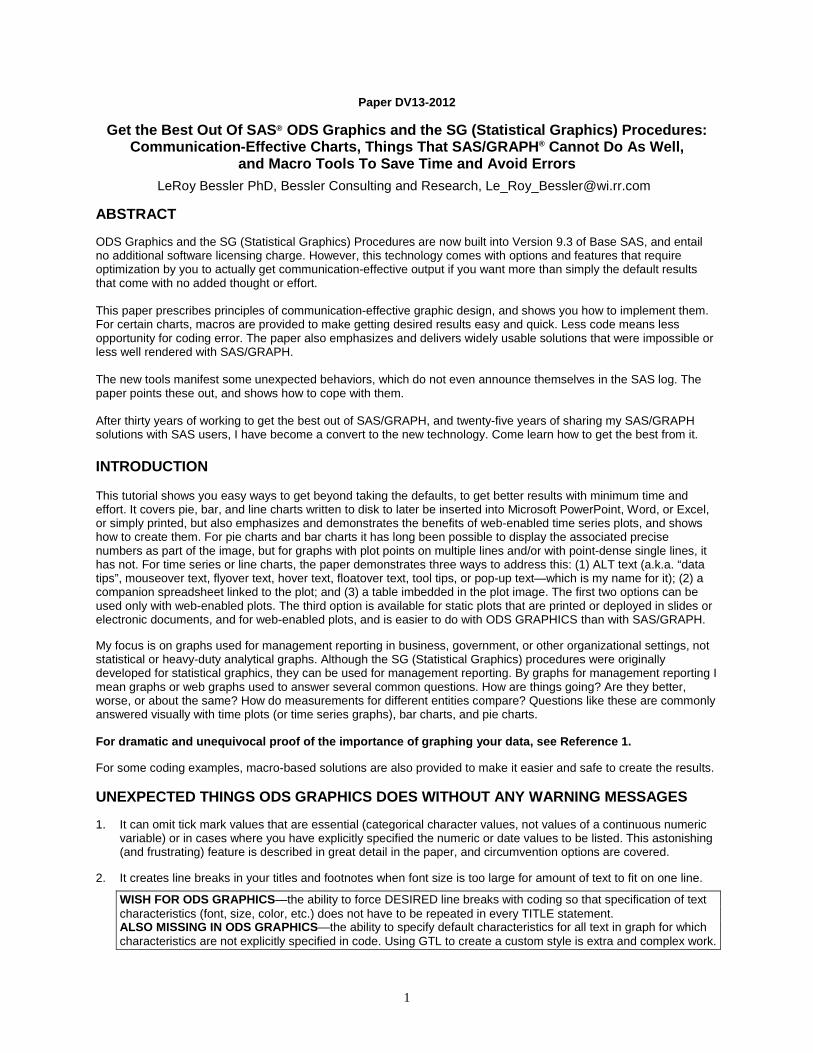
Communication-Effective Graphic Design Principle 4: Provide a reliably usable legend In graphs, legends are typically used to decode the identity of colored plot lines and markers or of color-filled bars or pie slices. The usability of a color-based legend is related to these insufficiently recognized facts of color communication. If you want to be able to reliably distinguish colors, then • colored text must be thick enough • colored lines must be thick enough • colored plot point markers must be large enough • colored samples, whether area fill, line segment, or plot point marker, in a legend must be large enough ODS Graphics does provide controls for thickness of lines and size of plot point markers. And that thickness and size also carry over into the legend for a plot. Unfortunately, there are no ODS Graphics controls for the size of the colored sample patches in bar chart legends. SAS/GRAPH provides that support. ODS Graphics does not. This same functional deficiency has always been present in Excel pie chart legends. The lack of control in ODS Graphics is disappointing.

7

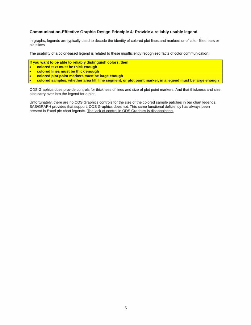
Communication-Effective Graphic Design Principle 5: Suppress and avoid graphic frills Let your data talk. ODS Graphics, unlike SAS/GRAPH, somewhat limits the user’s ability to inflict needless non-communicative or anti-communicative decoration (e.g., no 3D features for what are really two-variable 2D graphs). However, it does retain the standard graphic paraphernalia from the days when laboratory data was plotted with ink on grid paper. Coding to remove that paraphernalia is presented here later. Note About Color. One communication hazard is the ability to present text (numbers and/or letters) over colored areas or in a graph with a colored background. The most reliable text-background color combination is black and white. The standard format for books, newspapers, and magazines is not an accidental choice. If not using black and white, the text-background color combination should be high contrast, and not the color pair that is the indistinguishable for people with the commonest form of color blindness. For more about text and color, and much else about effective communication with color, see Reference 3. By the way, the color combination used in this note is a communication-effective choice. Why should you care about clutter? Here are miniature excerpts of some of my favorite slides to answer this. Complexity Distorts, Impedes, Delays Communication Simplicity - Powerful - Elegant Elegant - everything needed - only the needed sparse image focuses attention sparse graph more easily and more quickly interpreted When the fourth text item above is displayed as a slide, it is a powerful demonstration of what it says.

8

CLUTTER SUPPRESSION Before we FINALLY get to some graphs, let me quickly cover the easy how-to technical details of clutter suppression. Non-communicative graphic elements that I always remove are: • axis labels that can be in title or subtitle • axis lines • tick marks for tick values, especially if using grid lines • frame around graph detail area (which is not the Border around the entire graph) An axis of dates, times, or datetimes (unless exotically rendered in a hard-to-interpret format) NEVER needs a label. Coding methods to accomplish removal are: yaxis display=(nolabel); /* no axis label */ yaxis display=(noline) ; /* no axis line */ yaxis display=(noticks); /* no tick marks */ yaxis display=none; /* no label, no line, no tick marks */ Above also apply to xaxis, rowaxis, and colaxis. hbar . . . / . . . nooutline ; /* no bar outline */ Above also applies to vbar. The choice display=none might seem counterintuitive, but, if you have a bar chart with each bar end labeled with the response value (using the simple option of DATALABEL), there is absolutely No Reason to include a response axis. Nevertheless, this superfluity commonly appears in bar charts. ODS Graphics automatically encases the bars of a bar chart or the plot area of a plot in a frame. Unlike SAS/GRAPH, in the current version (9.3) of ODS Graphics there is no way to turn off the frame. Until the option is provided, if you wish to suppress the frame, you need to use a customized ODS style. If you do not routinely specify an ODS style for your output, you need to know what is the default style being applied by SAS to your ODS output: HTML – Styles.Default (formerly) HTML – Styles.HTMLblue (V9.3) RTF – Styles.Rtf PDF – Styles.Printer LISTING – Styles.Listing (NEW) If you are creating a graph on disk for later use, you need to use the ODS LISTING destination. If your base style is one of the above or one of the non-default choices supported by ODS, to be able to remove the graph work area frame, you need to first create a derived style with code like this: proc template; define style styles.YourStyleName; parent=styles.SomePreExistingStyle; class graphwalls / frameborder=off; end; run; When creating the graph, you must apply the style like this (for a graph on disk): ODS LISTING GPATH="YourTargetFolderLocation" STYLE=Styles.YourStyleName; ODS GRAPHICS ON / . . . IMAGENAME="YourDesiredFileName"; /* your SG procedure code goes here */ ODS LISTING CLOSE; ODS LISTING; NOTE: It is important to always close the LISTING destination (and to reopen it as shown). If you omit the close, the graph will be written to disk, but there can be unexpected effects in the next graph created in the same session.

9

PIE CHARTS: A Deservedly Popular Tool for Graphic Communication I understand that some statisticians, as well as some critics of graphic style, object to pie charts. Well, it is a fact that pie charts are one of the commonest graphic delivery instruments, regardless of ideological abstention in some venues and despite misconceptions about what is possible. If a pie chart is designed and executed well, there is no better way to visually compare the relative sizes of shares of the whole. Let’s proceed to achieve this, but starting from defaults, which DO deliver sub-optimal results. NOTE: For my most recent work pie charts, but in the context of SAS/GRAPH, see Reference 4.

10

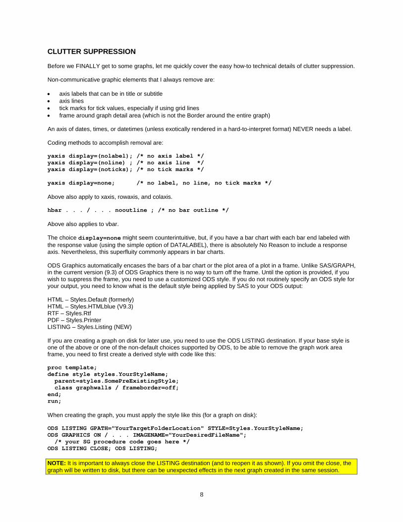
Unacceptable Default Pie Chart: NOT Communication-Effective for four reasons enumerated below.

1. Pie slices are ordered by label name, not by size. 2. “Other” withholds, rather than delivers, information. 3. The numeric values of percent share of the whole are not shown. 4. Some labels are outside, one label is inside. Failing to be able to order by size makes it cumbersome to identify the relative significance of the shares of the whole. This is NOT an inherent pie chart defect. It was a choice of the SAS ODS GRAPHICS software developer. The presence of an “Other” slice is an all too common pie chart practice. Any graph or other report should answer questions, not prompt them (like “What is IN ‘Other’?”) But see “Exploiting the Extremes of ‘Other’” in Reference 4. Graphs accelerate inference. Numbers are necessary for reliable inference. Pie chart slices should be accompanied by the numeric percents of the whole. Putting labels inside the pie slices causes two problems: (a) Black text on white background is maximally readable. Text on a color background is more difficult to read. (b) Slices are always more constricted than the while space outside the pie. This increases the difficulty of also

supplying the numeric percent of the whole. Software Problem: Instead of providing an SG procedure, or an SG procedure feature, to DIRECTLY create a pie chart, the software developers require users to get involved with GTL (Graphic Template Language), which is a less user-friendly tool. Here is the code used to create the pie chart above: proc template; define statgraph SASDefaultPieChart; begingraph; entrytitle "GTL Pie Chart of Shoe Sales by Region - SAS Default"; layout region; piechart category=Product response=Sales; endlayout; endgraph; end; run; ods listing gpath="D:\@MWSUG2012\Results"; ods graphics on / reset=all border=on height=300px width=800px imagename='SGRENDER_GTL_PieChart_SASDefault'; proc sgrender data=sashelp.shoes template=SASDefaultPieChart; run; ods listing close; ods listing;

11

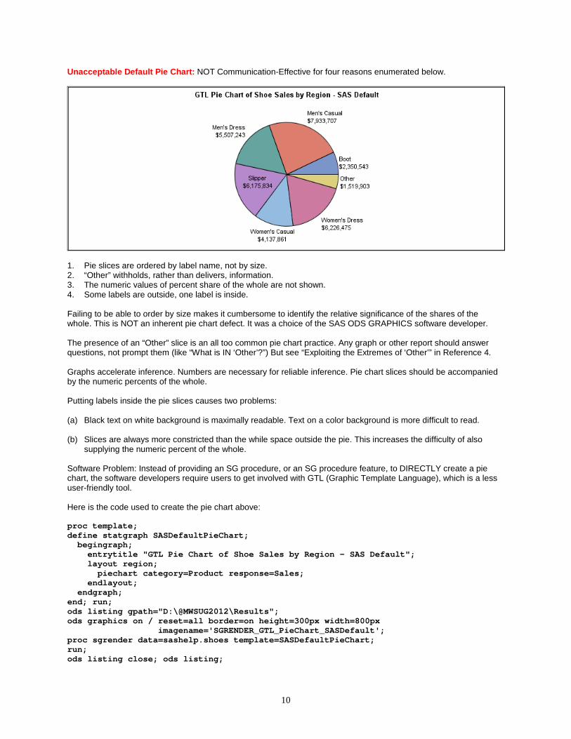
Better, But Not Best, Pie Chart: Pie slices are still ordered by label name, not size, and percent of whole is missing.

Better: All slice labels are now outside the pie, and all shoe styles are now explicitly identified—No “Other” permitted. Here is the code, now including two simple added parameters, used to create the pie chart above: proc template; define statgraph BesslerNearDefaultPieChart; begingraph; entrytitle "GTL Pie Chart - All Labels Outside & No 'Other' Slice"; layout region; piechart category=Product response=Sales / datalabellocation=outside otherslice=FALSE ; endlayout; endgraph; end; run; ods listing gpath="D:\@MWSUG2012\Results"; ods graphics on / reset=all border=on height=300px width=800px imagename='SGRENDER_GTL_PieChart_BesslerNearDefault'; proc sgrender data=sashelp.shoes template=BesslerNearDefaultPieChart; run; ods listing close; ods listing;

12

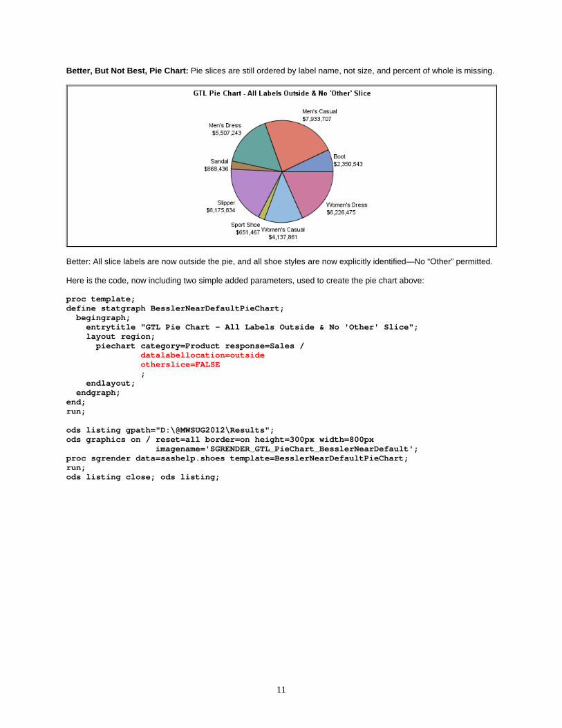
Best Pie Chart: Pie slices are ordered by size, and numeric percent of whole is now included in the slice labels.

Below is the more complicated code needed to create the pie chart above. Later in this paper, a macro solution is provided to make this easier and less vulnerable to possible error. proc summary data=sashelp.shoes nway; class Product; var Sales; output out=ToPrep sum=TotalByClass; run; proc sql noprint; select sum(TotalByClass) into :GrandTotal from ToPrep; quit; data ToChart; length SliceNameWithPercentAndValue $ 256; set ToPrep; SliceNameWithPercentAndValue = trim(left( put(((TotalByClass / &GrandTotal) * 100),z4.1) )) || '% - ' || trim(left(Product)) || ' - ' || trim(left(put(TotalByClass,dollar10.))); run; proc sort data=ToChart; by Descending TotalByClass; run; proc template; define statgraph BesslerBestPieChart31May2012; begingraph; entrytitle "GTL Pie Chart – Ordered and With Maximum Pie-Chart-Appropriate Information"; layout region; piechart category=SliceNameWithPercentAndValue response=TotalByClass / datalabelcontent=(category) datalabellocation=callout otherslice=FALSE; endlayout; endgraph; end; run;

13

ods listing gpath="D:\@MWSUG2012\Results"; ods graphics on / reset=all border=on height=300px width=800px imagename="BesslerBestPieChartCreatedNotUsingMacro"; proc sgrender data=ToChart template=BesslerBestPieChart31May2012; run; ods listing close; ods listing;

14

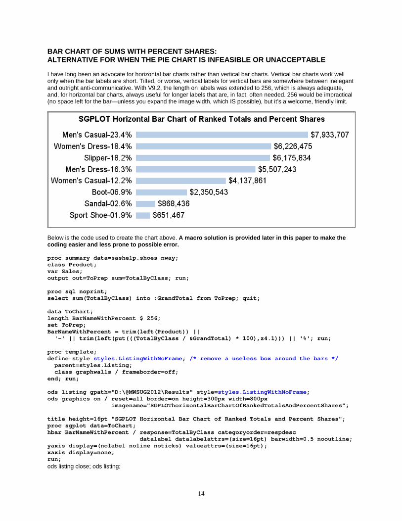
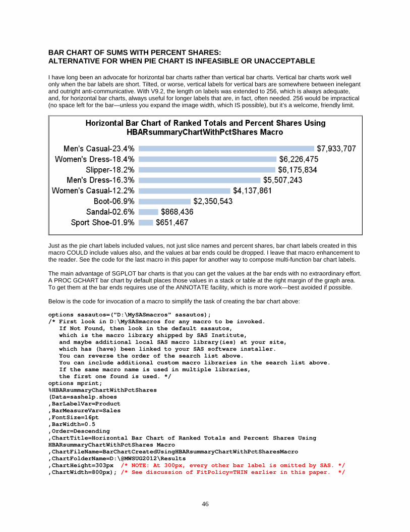
BAR CHART OF SUMS WITH PERCENT SHARES: ALTERNATIVE FOR WHEN THE PIE CHART IS INFEASIBLE OR UNACCEPTABLE I have long been an advocate for horizontal bar charts rather than vertical bar charts. Vertical bar charts work well only when the bar labels are short. Tilted, or worse, vertical labels for vertical bars are somewhere between inelegant and outright anti-communicative. With V9.2, the length on labels was extended to 256, which is always adequate, and, for horizontal bar charts, always useful for longer labels that are, in fact, often needed. 256 would be impractical (no space left for the bar—unless you expand the image width, which IS possible), but it’s a welcome, friendly limit.

Below is the code used to create the chart above. A macro solution is provided later in this paper to make the coding easier and less prone to possible error. proc summary data=sashelp.shoes nway; class Product; var Sales; output out=ToPrep sum=TotalByClass; run; proc sql noprint; select sum(TotalByClass) into :GrandTotal from ToPrep; quit; data ToChart; length BarNameWithPercent $ 256; set ToPrep; BarNameWithPercent = trim(left(Product)) || '-' || trim(left(put(((TotalByClass / &GrandTotal) * 100),z4.1))) || '%'; run; proc template; define style styles.ListingWithNoFrame; /* remove a useless box around the bars */ parent=styles.Listing; class graphwalls / frameborder=off; end; run; ods listing gpath="D:\@MWSUG2012\Results" style=styles.ListingWithNoFrame; ods graphics on / reset=all border=on height=300px width=800px imagename="SGPLOThorizontalBarChartOfRankedTotalsAndPercentShares"; title height=16pt "SGPLOT Horizontal Bar Chart of Ranked Totals and Percent Shares"; proc sgplot data=ToChart; hbar BarNameWithPercent / response=TotalByClass categoryorder=respdesc datalabel datalabelattrs=(size=16pt) barwidth=0.5 nooutline; yaxis display=(nolabel noline noticks) valueattrs=(size=16pt); xaxis display=none; run; ods listing close; ods listing;

15

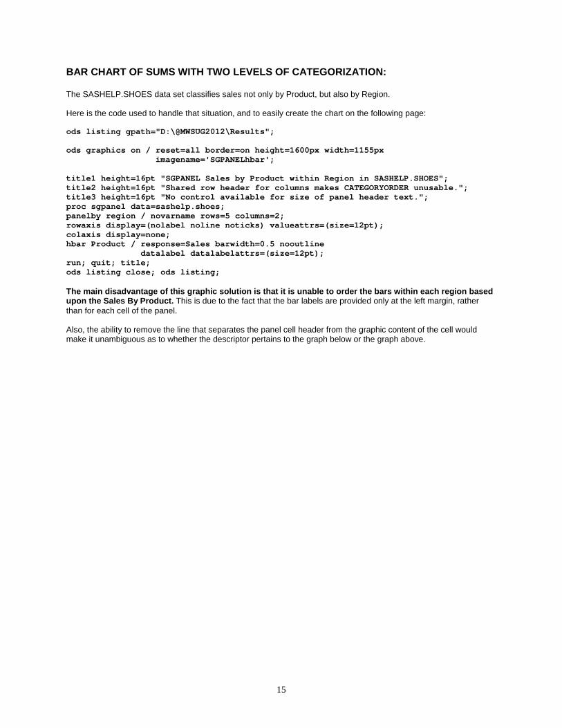
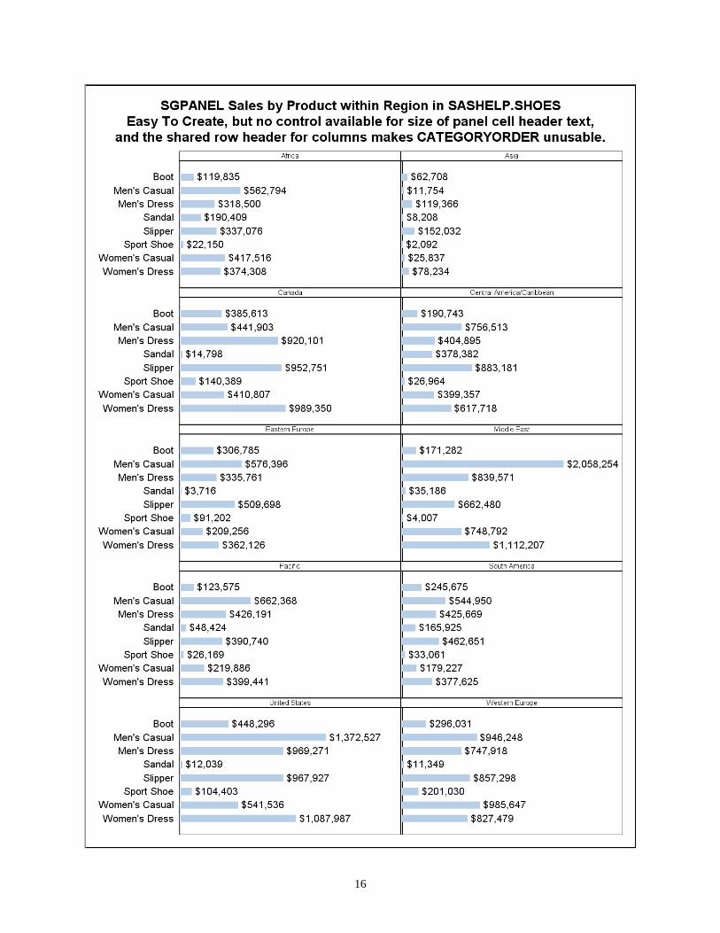
BAR CHART OF SUMS WITH TWO LEVELS OF CATEGORIZATION: The SASHELP.SHOES data set classifies sales not only by Product, but also by Region. Here is the code used to handle that situation, and to easily create the chart on the following page: ods listing gpath="D:\@MWSUG2012\Results"; ods graphics on / reset=all border=on height=1600px width=1155px imagename='SGPANELhbar'; title1 height=16pt "SGPANEL Sales by Product within Region in SASHELP.SHOES"; title2 height=16pt "Shared row header for columns makes CATEGORYORDER unusable."; title3 height=16pt "No control available for size of panel header text."; proc sgpanel data=sashelp.shoes; panelby region / novarname rows=5 columns=2; rowaxis display=(nolabel noline noticks) valueattrs=(size=12pt); colaxis display=none; hbar Product / response=Sales barwidth=0.5 nooutline datalabel datalabelattrs=(size=12pt); run; quit; title; ods listing close; ods listing; The main disadvantage of this graphic solution is that it is unable to order the bars within each region based upon the Sales By Product. This is due to the fact that the bar labels are provided only at the left margin, rather than for each cell of the panel. Also, the ability to remove the line that separates the panel cell header from the graphic content of the cell would make it unambiguous as to whether the descriptor pertains to the graph below or the graph above.

16

17

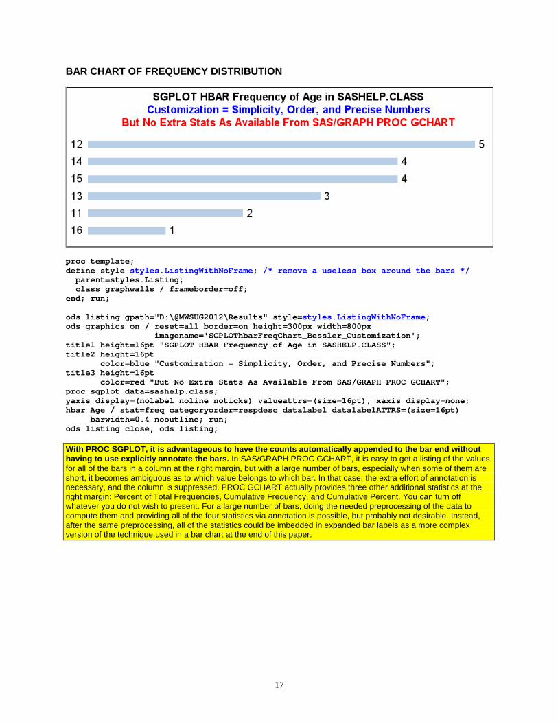
BAR CHART OF FREQUENCY DISTRIBUTION

proc template; define style styles.ListingWithNoFrame; /* remove a useless box around the bars */ parent=styles.Listing; class graphwalls / frameborder=off; end; run; ods listing gpath="D:\@MWSUG2012\Results" style=styles.ListingWithNoFrame; ods graphics on / reset=all border=on height=300px width=800px imagename='SGPLOThbarFreqChart_Bessler_Customization'; title1 height=16pt "SGPLOT HBAR Frequency of Age in SASHELP.CLASS"; title2 height=16pt color=blue "Customization = Simplicity, Order, and Precise Numbers"; title3 height=16pt color=red "But No Extra Stats As Available From SAS/GRAPH PROC GCHART"; proc sgplot data=sashelp.class; yaxis display=(nolabel noline noticks) valueattrs=(size=16pt); xaxis display=none; hbar Age / stat=freq categoryorder=respdesc datalabel datalabelATTRS=(size=16pt) barwidth=0.4 nooutline; run; ods listing close; ods listing; With PROC SGPLOT, it is advantageous to have the counts automatically appended to the bar end without having to use explicitly annotate the bars. In SAS/GRAPH PROC GCHART, it is easy to get a listing of the values for all of the bars in a column at the right margin, but with a large number of bars, especially when some of them are short, it becomes ambiguous as to which value belongs to which bar. In that case, the extra effort of annotation is necessary, and the column is suppressed. PROC GCHART actually provides three other additional statistics at the right margin: Percent of Total Frequencies, Cumulative Frequency, and Cumulative Percent. You can turn off whatever you do not wish to present. For a large number of bars, doing the needed preprocessing of the data to compute them and providing all of the four statistics via annotation is possible, but probably not desirable. Instead, after the same preprocessing, all of the statistics could be imbedded in expanded bar labels as a more complex version of the technique used in a bar chart at the end of this paper.

18

TIME PLOTS, TIME SERIES GRAPHS, TREND LINES, LINE CHARTS, etc. In SAS/GRAPH, the GPLOT procedure can visually present the evolution of data values over time. In ODS GRAPHICS, the SG procedures provide many more ways. In References 5 & 6, in collaboration with Alexandra Riley, I compared a variety of ways to visually present time series data using the old and new technology. In Reference 7, I provided more information about such plots and tools. One of the tools omitted in those prior works is the SERIES plot, which is the focus here. I use SERIES plots both with PROC SGPLOT and PROC SGPANEL. These examples use web-deployed graphs so that ALT text can be provided, rather than forcing the viewer to guess y and x values based on tick mark values at the axes. Another solution for time series, first developed with SAS/GRAPH in Reference 2 and adapted to ODS GRAPHICS later in this paper, is to link the plot forwards and backwards with a spreadsheet. NOTE 1: Most of the illustrations in this section are inserted PNG files, not screen prints of the web graphs from a web browser window. However, all code does create the web-enabling HTML for the graphs. NOTE 2: These examples require that the code in Appendix 1 be run first to prepare the input data. In PROC GPLOT, DESCRIPTION=' ' can be used on the PLOT statement used in order to prevent the display of the default pop-up text that tries to describe the graph when you rest the mouse anywhere in the graph area on the web page. Or you can use it to provide a custom description to replace the default. For Statistical Graphics procedures, the default description can neither be nullified nor customized. These pop-up descriptions can be a nuisance when you want to instead display the ALT text for the plot points. The ALT text for PROC GPLOT is provided via the PLOT statement’s HTML parameter, which identifies a variable on the plot input data set. The variable can be customized with anything the designer/programmer desires, including line breaks, any text, the plot point values in any format to any precision, and times, datetimes, or dates in any format that you prefer (e.g., dates formatted with day of the week name, as well as month, day, year). For Statistical Graphics procedures, ALT text is triggered by IMAGEMAP=ON in an ODS GRAPHICS statement. The text displayed is simply a list of the form Variable Name (or Label) = Value, and cannot be customized. For these graphs, the data used is SASHELP.CITIDAY, which is shipped with SAS/ETS. It contains daily history for financial market and other economic information. If you don’t have SAS/ETS, you can ask SAS Technical Support for how to download the data set. The data used here is limited to year 1990. Since the best way to determine the precise value of the Dow index in these web-enabled plots is from the pop-up ALT text, in these graphs I display along the y axis only the minimum and maximum values for the Dow.

19

INTRODUCTION TO THE TIME SERIES EXAMPLES: DISCUSSION OF STATEMENTS AND PARAMETERS Statements Common to All of the Time Series Charts ods graphics on / reset=all /* Suppress any leftovers from prior code runs */ border=off /* Not usually desired on a web page but turn on if wanting to see how much extra space might be available in the browser window for a wider image */ antialiasmax=2500 /* antialiasing is on by default, but antialiasmax is defaulted to 600. If that is insufficient, then antialiasing will be incomplete */ tipmax=2500 /* This is the maximum number of distinct mouse-over areas allowed before data tips are disabled. Default is 400. */ imagemap=on /* This turns on the data tips. SAS/GRAPH allows customization of the data tips, but ODS GRAPHICS does not. */ imagename='DesiredFileNameForThePNGimageFile'; yaxis display=(nolabel) /* the yaxis variable is identified in the plot title */ values=(&Ymin_1990 &Ymax_1990); /* show only the yaxis minimum and maximum, available as symbolic (or macro) variables from setup processing. */ xaxis display=(nolabel) /* the xaxis variable is identified in the plot title */ grid /* provide reference lines for each xaxis tick mark value */ . . . /* here specify a list of values or (see below) Interval= */ Example Assignments for Parameters Added to ODS GRAPHICS Statement for Some Series Charts width=800px /* width of image in pixels, default is 640 */ height=600px /* height of image in pixels, default is 480 */ If your target is HTML (web page), your choice of dimensions should rarely, if ever, exceed the dimensions of the available live space in the browser and monitor likely to be used. Live Space is the viewable display area WITHOUT scrolling. The usability of a graph is diminished if it needs to be scrolled. Typical (but not All) Parameters Used on SERIES Statement in This Paper series y=YourYAXISvar x=YourXAXISvar / markers /* turns on plot-point markers default is nomarkers */ markerattrs=(size=7 symbol=circlefilled color=red /* But DO NOT specify a color if using GROUP= on the SERIES statement to produce a multi-line overlay */ ) lineattrs=(thickness=N /* where, in this paper, N is 2 or 3. 3 is used when chart has multiple lines (as in the twelve months of 1990 overlaid) so that line colors are more easily distinguished */ pattern=solid /* If you do not specify your pattern preference, the software might make a decision for you, which you might not like. */ color=blue /* But DO NOT specify a color if using GROUP= on the SERIES statement to produce a multi-line overlay */ );

20

Parameters of Special Interest on the XAXIS Statement For Date, Time, or DateTime Variables: Interval= can have numerous different values. Used here are MONTH, SEMIMONTH, and WEEK. In some graphs here, the XAXIS variable is Day Of Month, which is not a Date. There Interval= does not apply. For Any Variable: FitPolicy= defaults to THIN, which means that an ODS GRAPHICS SG procedure will OMIT any tick mark values that it cannot fit (based on its estimates, which CAN BE wrong). Also, it does this omission with no message in the SAS log, even if you have explicitly specified a list of tick mark values to be displayed with the VALUES= parameter or have certain expectations based on what you might have specified with the INTERVAL= parameter. When the displayed tick mark values are fewer than what you would like, there are five options: increase the width of the image if the xaxis has the problem specify FitPolicy=Stagger specify FitPolicy=StaggerRotate (first try Stagger, if no help, use Rotate) specify FitPolicy=RotateStagger (first try Rotate, if no help, use Stagger) specify FitPolicy=Rotate (least desirable) NOTE: When a yaxis set of values is thinned, if that causes a problem, your only option is to increase the height of the image. If the yaxis variable has discrete character values, thinning is absolutely unacceptable.

21

TIME SERIES EXAMPLES: ALL USING THE SERIES STATEMENT, WITH PROC SGPANEL OR PROC SGPLOT All examples use Dow Index data for one year of trading days in 1990 One of these uses PROC SGPANEL which creates an array of subplots for segments of the time period. In the case presented here, it is an array of the twelve months of year 1990. The remaining examples all use PROC SGPLOT. If GROUP=MONTH is added to the SERIES statement, the twelve months are plotted as separate lines in an overlay. Without GROUP=MONTH, the data is plotted as one line. The last example demonstrates a plot and spreadsheet hyperlinked to each other forwards and backwards. ALT text (aka “data tips”) on the web-deployed plot DOES make precise numbers available for temporary look-up, but the spreadsheet makes them available both for casual inspection as a whole, and for reuse with Excel however the user of the deliverable sees fit to explore or further manipulate the data. For non-web-enabled plots, the section after this one shows how to imbed the precise y values inside a plot image area by using SGPLOT with a VLINE statement instead of the SERIES statement, which is the focus of this section. The y values can be imbedded as either a table between the plot lines and x axis or as direct plot-point annotation.

22

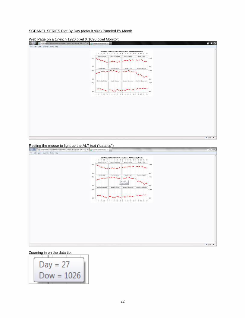
SGPANEL SERIES Plot By Day (default size) Paneled By Month Web Page on a 17-inch 1920 pixel X 1090 pixel Monitor:

Resting the mouse to light up the ALT text (“data tip”)

Zooming in on the data tip:

23

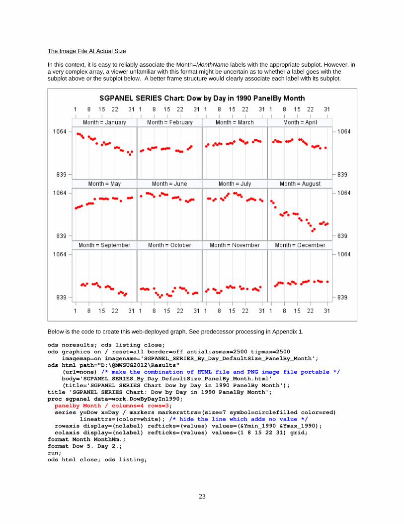
The Image File At Actual Size In this context, it is easy to reliably associate the Month=MonthName labels with the appropriate subplot. However, in a very complex array, a viewer unfamiliar with this format might be uncertain as to whether a label goes with the subplot above or the subplot below. A better frame structure would clearly associate each label with its subplot.

Below is the code to create this web-deployed graph. See predecessor processing in Appendix 1. ods noresults; ods listing close; ods graphics on / reset=all border=off antialiasmax=2500 tipmax=2500 imagemap=on imagename='SGPANEL_SERIES_By_Day_DefaultSize_PanelBy_Month'; ods html path="D:\@MWSUG2012\Results" (url=none) /* make the combination of HTML file and PNG image file portable */ body='SGPANEL_SERIES_By_Day_DefaultSize_PanelBy_Month.html' (title='SGPANEL SERIES Chart Dow by Day in 1990 PanelBy Month'); title 'SGPANEL SERIES Chart: Dow by Day in 1990 PanelBy Month'; proc sgpanel data=work.DowByDayIn1990; panelby Month / columns=4 rows=3; series y=Dow x=Day / markers markerattrs=(size=7 symbol=circlefilled color=red) lineattrs=(color=white); /* hide the line which adds no value */ rowaxis display=(nolabel) refticks=(values) values=(&Ymin_1990 &Ymax_1990); colaxis display=(nolabel) refticks=(values) values=(1 8 15 22 31) grid; format Month MonthNm.; format Dow 5. Day 2.; run; ods html close; ods listing;

24

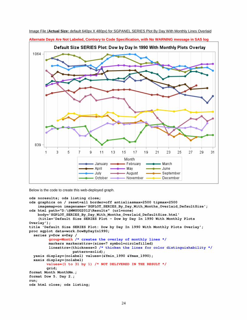
Image File (Actual Size: default 640px X 480px) for SGPANEL SERIES Plot By Day With Monthly Lines Overlaid Alternate Days Are Not Labeled, Contrary to Code Specification, with No WARNING message in SAS log

Below is the code to create this web-deployed graph. ods noresults; ods listing close; ods graphics on / reset=all border=off antialiasmax=2500 tipmax=2500 imagemap=on imagename='SGPLOT_SERIES_By_Day_With_Months_Overlaid_DefaultSize'; ods html path="D:\@MWSUG2012\Results" (url=none) body='SGPLOT_SERIES_By_Day_With_Months_Overlaid_DefaultSize.html' (title='Default Size SERIES Plot - Dow by Day In 1990 With Monthly Plots Overlay'); title 'Default Size SERIES Plot: Dow by Day In 1990 With Monthly Plots Overlay'; proc sgplot data=work.DowByDayIn1990; series y=Dow x=Day / group=Month /* creates the overlay of monthly lines */ markers markerattrs=(size=7 symbol=circlefilled) lineattrs=(thickness=3 /* thicken the lines for color distinguishability */ pattern=solid); yaxis display=(nolabel) values=(&Ymin_1990 &Ymax_1990); xaxis display=(nolabel) values=(1 to 31 by 1) /* NOT DELIVERED IN THE RESULT */ grid; format Month MonthNm.; format Dow 5. Day 2.; run; ods html close; ods listing;

25

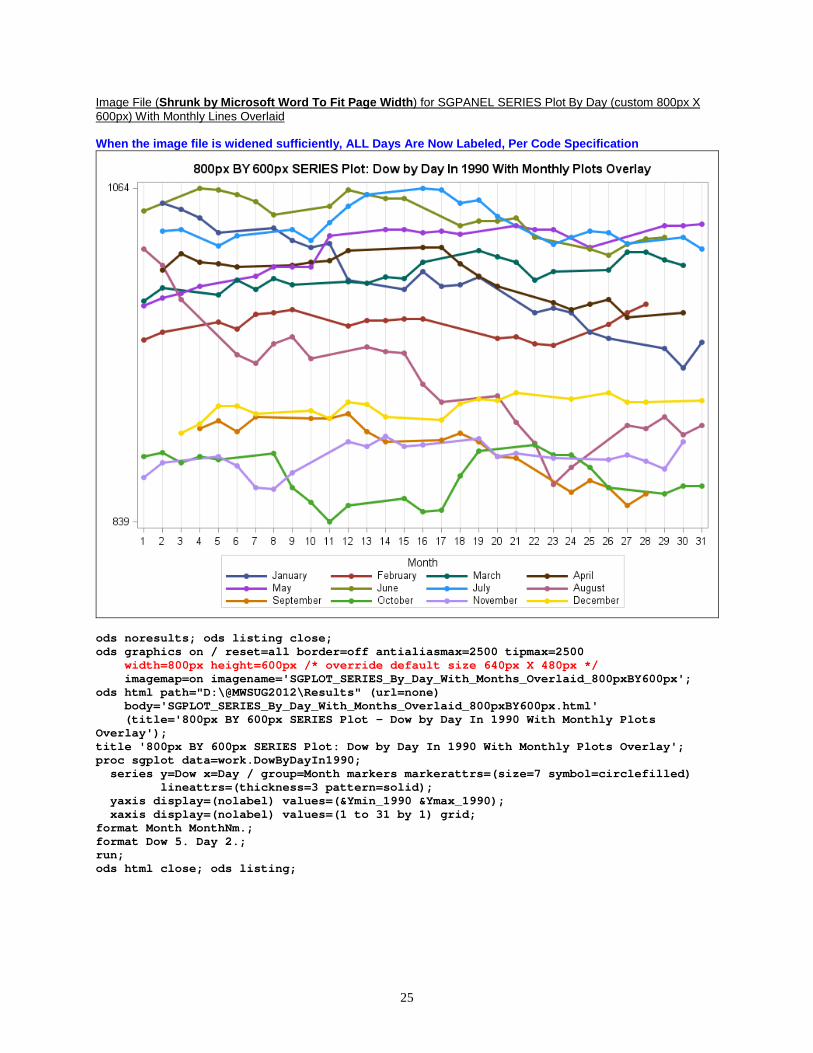
Image File (Shrunk by Microsoft Word To Fit Page Width) for SGPANEL SERIES Plot By Day (custom 800px X 600px) With Monthly Lines Overlaid When the image file is widened sufficiently, ALL Days Are Now Labeled, Per Code Specification

ods noresults; ods listing close; ods graphics on / reset=all border=off antialiasmax=2500 tipmax=2500 width=800px height=600px /* override default size 640px X 480px */ imagemap=on imagename='SGPLOT_SERIES_By_Day_With_Months_Overlaid_800pxBY600px'; ods html path="D:\@MWSUG2012\Results" (url=none) body='SGPLOT_SERIES_By_Day_With_Months_Overlaid_800pxBY600px.html' (title='800px BY 600px SERIES Plot - Dow by Day In 1990 With Monthly Plots Overlay'); title '800px BY 600px SERIES Plot: Dow by Day In 1990 With Monthly Plots Overlay'; proc sgplot data=work.DowByDayIn1990; series y=Dow x=Day / group=Month markers markerattrs=(size=7 symbol=circlefilled) lineattrs=(thickness=3 pattern=solid); yaxis display=(nolabel) values=(&Ymin_1990 &Ymax_1990); xaxis display=(nolabel) values=(1 to 31 by 1) grid; format Month MonthNm.; format Dow 5. Day 2.; run; ods html close; ods listing;

26

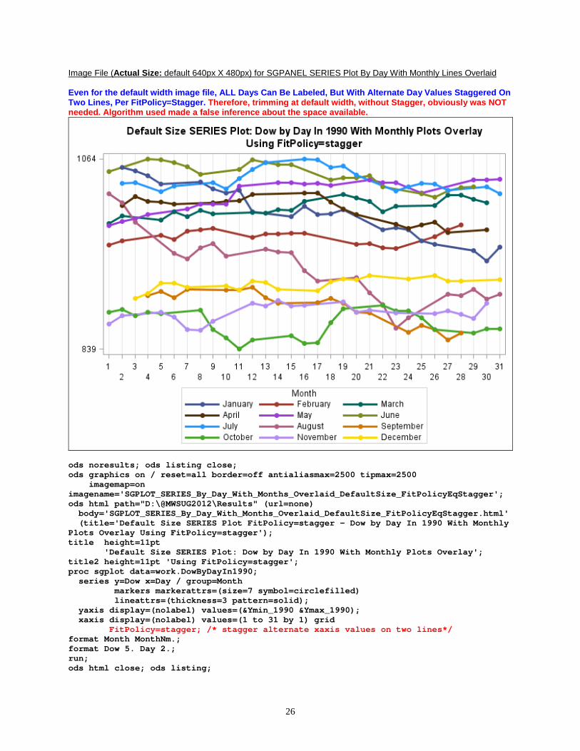
Image File (Actual Size: default 640px X 480px) for SGPANEL SERIES Plot By Day With Monthly Lines Overlaid Even for the default width image file, ALL Days Can Be Labeled, But With Alternate Day Values Staggered On Two Lines, Per FitPolicy=Stagger. Therefore, trimming at default width, without Stagger, obviously was NOT needed. Algorithm used made a false inference about the space available.

ods noresults; ods listing close; ods graphics on / reset=all border=off antialiasmax=2500 tipmax=2500 imagemap=on imagename='SGPLOT_SERIES_By_Day_With_Months_Overlaid_DefaultSize_FitPolicyEqStagger'; ods html path="D:\@MWSUG2012\Results" (url=none) body='SGPLOT_SERIES_By_Day_With_Months_Overlaid_DefaultSize_FitPolicyEqStagger.html' (title='Default Size SERIES Plot FitPolicy=stagger - Dow by Day In 1990 With Monthly Plots Overlay Using FitPolicy=stagger'); title height=11pt 'Default Size SERIES Plot: Dow by Day In 1990 With Monthly Plots Overlay'; title2 height=11pt 'Using FitPolicy=stagger'; proc sgplot data=work.DowByDayIn1990; series y=Dow x=Day / group=Month markers markerattrs=(size=7 symbol=circlefilled) lineattrs=(thickness=3 pattern=solid); yaxis display=(nolabel) values=(&Ymin_1990 &Ymax_1990); xaxis display=(nolabel) values=(1 to 31 by 1) grid FitPolicy=stagger; /* stagger alternate xaxis values on two lines*/ format Month MonthNm.; format Dow 5. Day 2.; run; ods html close; ods listing;

27

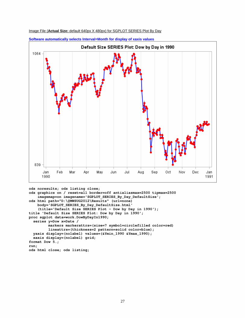
Image File (Actual Size: default 640px X 480px) for SGPLOT SERIES Plot By Day Software automatically selects Interval=Month for display of xaxis values

ods noresults; ods listing close; ods graphics on / reset=all border=off antialiasmax=2500 tipmax=2500 imagemap=on imagename='SGPLOT_SERIES_By_Day_DefaultSize'; ods html path="D:\@MWSUG2012\Results" (url=none) body='SGPLOT_SERIES_By_Day_DefaultSize.html' (title='Default Size SERIES Plot - Dow by Day in 1990'); title 'Default Size SERIES Plot: Dow by Day in 1990'; proc sgplot data=work.DowByDayIn1990; series y=Dow x=Date / markers markerattrs=(size=7 symbol=circlefilled color=red) lineattrs=(thickness=2 pattern=solid color=blue); yaxis display=(nolabel) values=(&Ymin_1990 &Ymax_1990); xaxis display=(nolabel) grid; format Dow 5.; run; ods html close; ods listing;

28

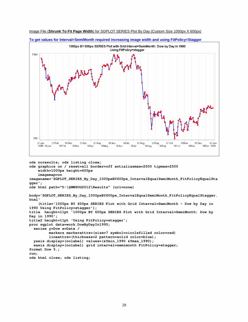
Image File (Shrunk To Fit Page Width) for SGPLOT SERIES Plot By Day (Custom Size 1000px X 600px) To get values for Interval=SemiMonth required increasing image width and using FitPolicy=Stagger

ods noresults; ods listing close; ods graphics on / reset=all border=off antialiasmax=2500 tipmax=2500 width=1000px height=600px imagemap=on imagename='SGPLOT_SERIES_By_Day_1000pxBY600px_IntervalEqualSemiMonth_FitPolicyEqualStagger'; ods html path="D:\@MWSUG2012\Results" (url=none) body='SGPLOT_SERIES_By_Day_1000pxBY600px_IntervalEqualSemiMonth_FitPolicyEqualStagger.html' (title='1000px BY 600px SERIES Plot with Grid Interval=SemiMonth - Dow by Day in 1990 Using FitPolicy=stagger'); title height=11pt '1000px BY 600px SERIES Plot with Grid Interval=SemiMonth: Dow by Day in 1990'; title2 height=11pt 'Using FitPolicy=stagger'; proc sgplot data=work.DowByDayIn1990; series y=Dow x=Date / markers markerattrs=(size=7 symbol=circlefilled color=red) lineattrs=(thickness=2 pattern=solid color=blue); yaxis display=(nolabel) values=(&Ymin_1990 &Ymax_1990); xaxis display=(nolabel) grid interval=semimonth FitPolicy=stagger; format Dow 5.; run; ods html close; ods listing;

29

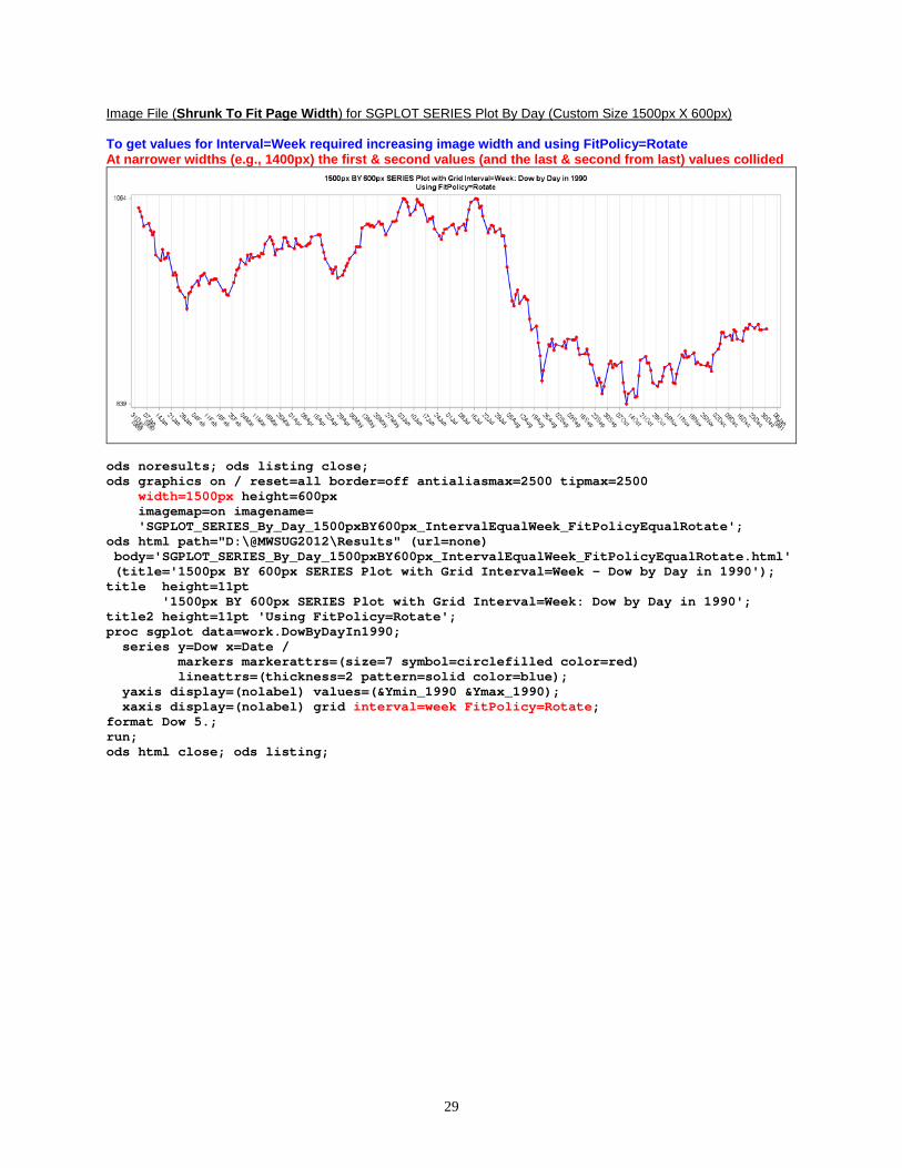
Image File (Shrunk To Fit Page Width) for SGPLOT SERIES Plot By Day (Custom Size 1500px X 600px) To get values for Interval=Week required increasing image width and using FitPolicy=Rotate At narrower widths (e.g., 1400px) the first & second values (and the last & second from last) values collided

ods noresults; ods listing close; ods graphics on / reset=all border=off antialiasmax=2500 tipmax=2500 width=1500px height=600px imagemap=on imagename= 'SGPLOT_SERIES_By_Day_1500pxBY600px_IntervalEqualWeek_FitPolicyEqualRotate'; ods html path="D:\@MWSUG2012\Results" (url=none) body='SGPLOT_SERIES_By_Day_1500pxBY600px_IntervalEqualWeek_FitPolicyEqualRotate.html' (title='1500px BY 600px SERIES Plot with Grid Interval=Week - Dow by Day in 1990'); title height=11pt '1500px BY 600px SERIES Plot with Grid Interval=Week: Dow by Day in 1990'; title2 height=11pt 'Using FitPolicy=Rotate'; proc sgplot data=work.DowByDayIn1990; series y=Dow x=Date / markers markerattrs=(size=7 symbol=circlefilled color=red) lineattrs=(thickness=2 pattern=solid color=blue); yaxis display=(nolabel) values=(&Ymin_1990 &Ymax_1990); xaxis display=(nolabel) grid interval=week FitPolicy=Rotate; format Dow 5.; run; ods html close; ods listing;

30

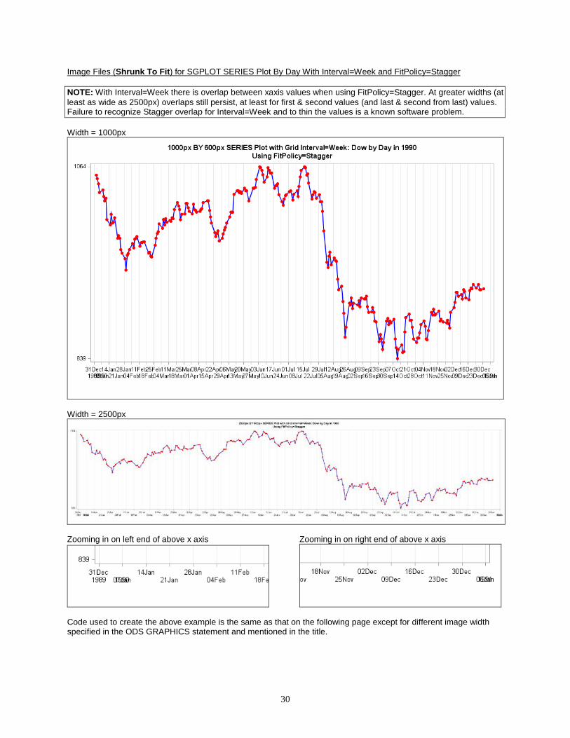
Image Files (Shrunk To Fit) for SGPLOT SERIES Plot By Day With Interval=Week and FitPolicy=Stagger NOTE: With Interval=Week there is overlap between xaxis values when using FitPolicy=Stagger. At greater widths (at least as wide as 2500px) overlaps still persist, at least for first & second values (and last & second from last) values. Failure to recognize Stagger overlap for Interval=Week and to thin the values is a known software problem. Width = 1000px

Width = 2500px

Zooming in on left end of above x axis Zooming in on right end of above x axis

Code used to create the above example is the same as that on the following page except for different image width specified in the ODS GRAPHICS statement and mentioned in the title.

31

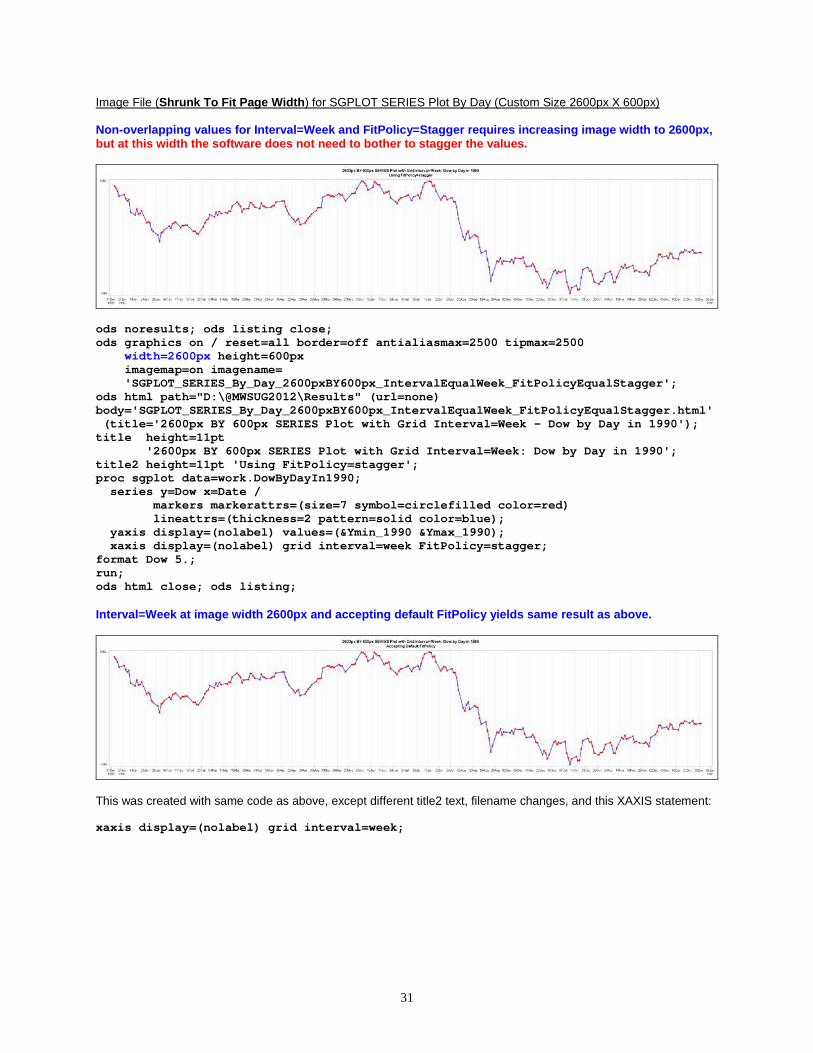
Image File (Shrunk To Fit Page Width) for SGPLOT SERIES Plot By Day (Custom Size 2600px X 600px) Non-overlapping values for Interval=Week and FitPolicy=Stagger requires increasing image width to 2600px, but at this width the software does not need to bother to stagger the values.

ods noresults; ods listing close; ods graphics on / reset=all border=off antialiasmax=2500 tipmax=2500 width=2600px height=600px imagemap=on imagename= 'SGPLOT_SERIES_By_Day_2600pxBY600px_IntervalEqualWeek_FitPolicyEqualStagger'; ods html path="D:\@MWSUG2012\Results" (url=none) body='SGPLOT_SERIES_By_Day_2600pxBY600px_IntervalEqualWeek_FitPolicyEqualStagger.html' (title='2600px BY 600px SERIES Plot with Grid Interval=Week - Dow by Day in 1990'); title height=11pt '2600px BY 600px SERIES Plot with Grid Interval=Week: Dow by Day in 1990'; title2 height=11pt 'Using FitPolicy=stagger'; proc sgplot data=work.DowByDayIn1990; series y=Dow x=Date / markers markerattrs=(size=7 symbol=circlefilled color=red) lineattrs=(thickness=2 pattern=solid color=blue); yaxis display=(nolabel) values=(&Ymin_1990 &Ymax_1990); xaxis display=(nolabel) grid interval=week FitPolicy=stagger; format Dow 5.; run; ods html close; ods listing; Interval=Week at image width 2600px and accepting default FitPolicy yields same result as above.

This was created with same code as above, except different title2 text, filename changes, and this XAXIS statement: xaxis display=(nolabel) grid interval=week;

32

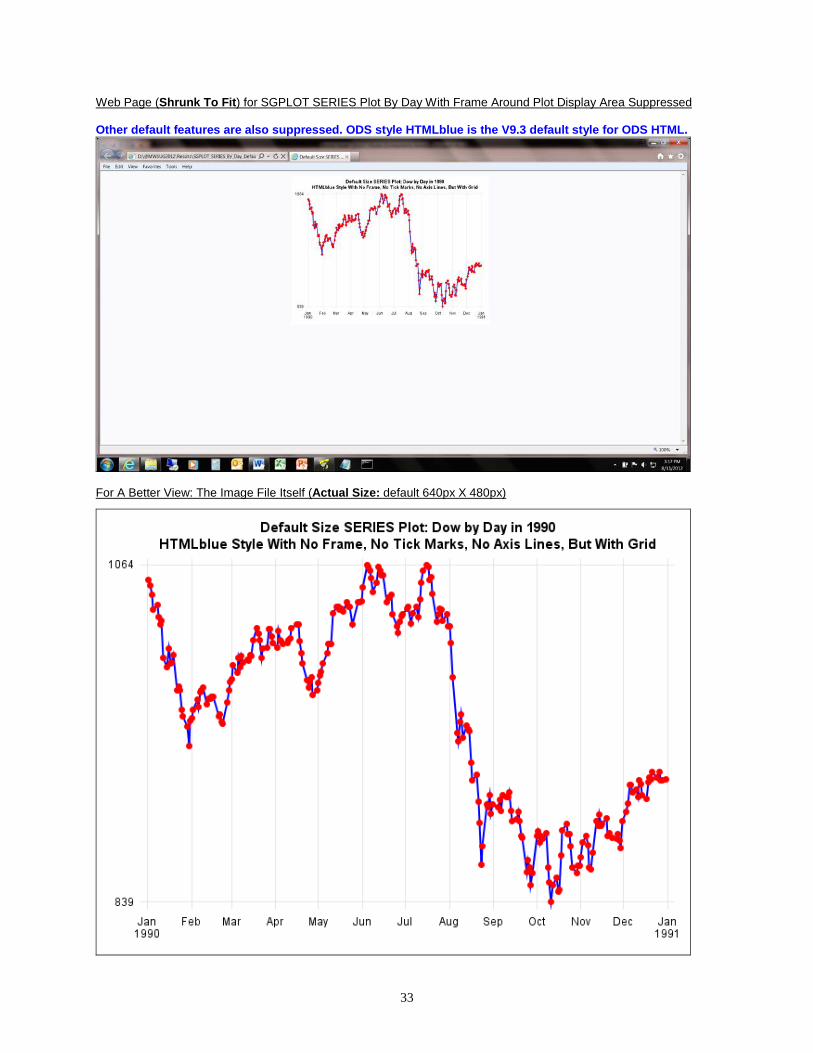
Simplifying the Appearance of the SERIES Plot Though necessary tick mark values, and sometimes grid lines, provide communication value, the little tick marks themselves, the axis lines, and any framing of the plot area add NO communication value. In PROC SGPLOT it is easy to turn off the tick marks, and OSTENSIBLY, the axis lines, but it is cumbersome to remove the frame. With the frame still present, the suppressed axis lines are overlaid with the four-sided frame, in which case the absence of axis lines is not apparent. It is my understanding that in SAS Version 9.4 it will be possible to remove the frame around the graph display area with an option, so that it will no longer be necessary to create a customized style to accomplish that. That capability is not be confused with ODS GRAPHICS ON / BORDER=OFF which is used to turn off the border around the entire image, not around the display area that contains the plot. Here is the code used to do the frame removal for the web graph displayed on the following page: proc template; define style styles.HTMLblueWithNoFrame; /* remove useless box around the plot area */ parent=styles.HTMLblue; class graphwalls / frameborder=off; end; run; ods noresults; ods listing close; ods graphics on / reset=all border=off antialiasmax=2500 tipmax=2500 imagemap=on imagename='SGPLOT_SERIES_By_Day_DefaultSize_HTMLblueStyle_WithNoFrame'; ods html path="D:\@MWSUG2012\Results" (url=none) style=styles.HTMLblueWithNoFrame body='SGPLOT_SERIES_By_Day_DefaultSize_HTMLblueStyle_WithNoFrame.html' (title='Default Size SERIES Plot - Dow by Day in 1990'); title1 height=11pt 'Default Size SERIES Plot: Dow by Day in 1990'; title2 height=11pt 'HTMLblue Style With No Frame, No Tick Marks, No Axis Lines, But With Grids'; proc sgplot data=work.DowByDayIn1990; series y=Dow x=Date / markers markerattrs=(size=7 symbol=circlefilled color=red) lineattrs=(thickness=2 pattern=solid color=blue); yaxis display=(nolabel noticks noline) grid values=(&Ymin_1990 &Ymax_1990); xaxis display=(nolabel noticks noline) grid; format Dow 5.; run; ods html close; ods listing;

33

Web Page (Shrunk To Fit) for SGPLOT SERIES Plot By Day With Frame Around Plot Display Area Suppressed Other default features are also suppressed. ODS style HTMLblue is the V9.3 default style for ODS HTML.

For A Better View: The Image File Itself (Actual Size: default 640px X 480px)

34

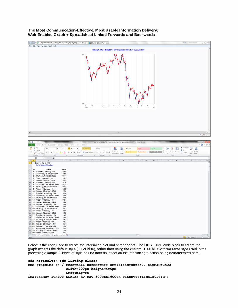
The Most Communication-Effective, Most Usable Information Delivery: Web-Enabled Graph + Spreadsheet Linked Forwards and Backwards

Below is the code used to create the interlinked plot and spreadsheet. The ODS HTML code block to create the graph accepts the default style (HTMLblue), rather than using the custom HTMLblueWithNoFrame style used in the preceding example. Choice of style has no material effect on the interlinking function being demonstrated here. ods noresults; ods listing close; ods graphics on / reset=all border=off antialiasmax=2500 tipmax=2500 width=800px height=600px imagemap=on imagename='SGPLOT_SERIES_By_Day_800pxBY600px_WithHyperLinkInTitle';

35

ods html path="D:\@MWSUG2012\Results" (url=none) nogtitle body='SGPLOT_SERIES_By_Day_800pxBY600px_WithHyperLinkInTitle.html' (title='800px BY 600px SERIES Plot With Hyperlink In Title - Dow by Day in 1990'); title link='D:\@MWSUG2012\Results\SGPLOT_SERIES_By_Day_SpreadSheet_WithHyperLinkInTitle.xls' '800px BY 600px SERIES Plot With Hyperlink In Title: Dow by Day in 1990'; proc sgplot data=work.DowByDayIn1990; series y=Dow x=Date / markers markerattrs=(size=7 symbol=circlefilled color=red) lineattrs=(thickness=2 pattern=solid); yaxis display=(nolabel) values=(&Ymin_1990 &Ymax_1990); xaxis display=(nolabel) grid; format Dow 5.; run; ods html close; ods html path="D:\@MWSUG2012\Results" body='SGPLOT_SERIES_By_Day_SpreadSheet_WithHyperLinkInTitle.xls'; title justify=left "<td COLSPAN=4>Dow by Day in 1990</td>" justify=left "<td COLSPAN=4> <a href='SGPLOT_SERIES_By_Day_800pxBY600px_WithHyperLinkInTitle.html'> Go To Graph of This Data</a></td>"; proc print data=work.DowByDayIn1990; var Date Dow; format Dow 5. Date weekdatx.; run; ods html close; ods listing;

36

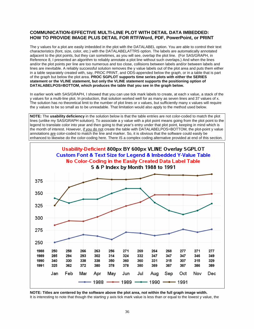
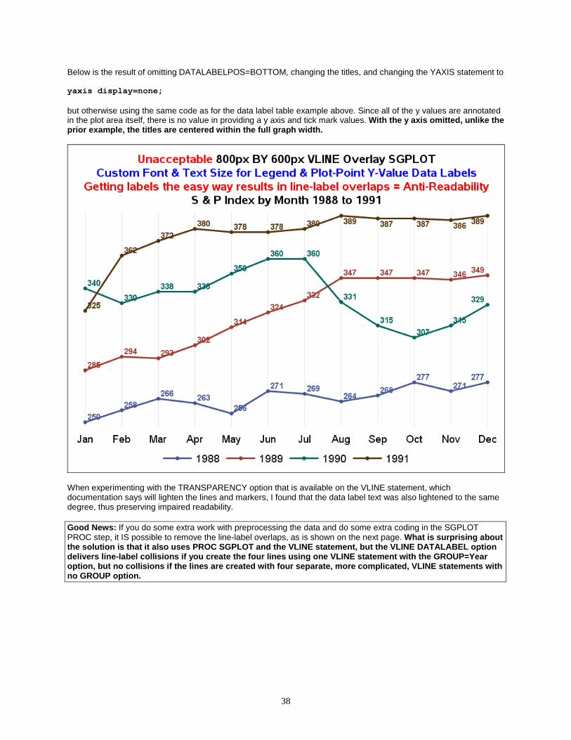
COMMUNICATION-EFFECTIVE MULTI-LINE PLOT WITH DETAIL DATA IMBEDDED: HOW TO PROVIDE IMAGE PLUS DETAIL FOR RTF/Word, PDF, PowerPoint, or PRINT The y values for a plot are easily imbedded in the plot with the DATALABEL option. You are able to control their text characteristics (font, size, color, etc.) with the DATALABELATTRS option. The labels are automatically annotated adjacent to the plot points, but they can sometimes, as you will see, overlap the plot line. (For SAS/GRAPH, in Reference 8, I presented an algorithm to reliably annotate a plot line without such overlaps.) And when the lines and/or the plot points per line are too numerous and too close, collisions between labels and/or between labels and lines are inevitable. A reliably successful solution removes the y value labels out of the plot area and puts them either in a table separately created with, say, PROC PRINT, and ODS-appended below the graph, or in a table that is part of the graph but below the plot area. PROC SGPLOT supports time series plots with either the SERIES statement or the VLINE statement, but only the VLINE statement supports the positioning option of DATALABELPOS=BOTTOM, which produces the table that you see in the graph below. In earlier work with SAS/GRAPH, I showed that you can use tick mark labels to create, at each x value, a stack of the y values for a multi-line plot. In production, that solution worked well for as many as seven lines and 37 values of x. The solution has no theoretical limit to the number of plot lines or x values, but sufficiently many x values will require the y values to be so small as to be unreadable. That limitation would also apply to the method used below. NOTE: The usability deficiency in the solution below is that the table entries are not color-coded to match the plot lines (unlike my SAS/GRAPH solution). To associate a y value with a plot point means going from the plot point to the legend to translate color into year and then going to that year’s entry under that plot point, keeping in mind which is the month of interest. However, if you do not create the table with DATALABELPOS=BOTTOM, the plot-point y value annotations are color-coded to match the line and marker. So, it is obvious that the software could easily be enhanced to likewise do the color-coding here. There IS a complex coding alternative provided at end of this section.

NOTE: Titles are centered by the software above the plot area, not within the full graph image width. It is interesting to note that though the starting y axis tick mark value is less than or equal to the lowest y value, the

37

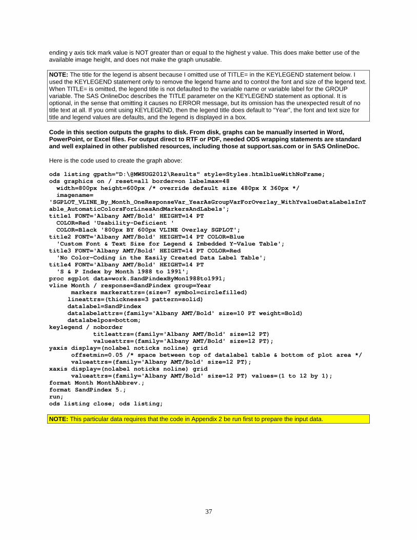
ending y axis tick mark value is NOT greater than or equal to the highest y value. This does make better use of the available image height, and does not make the graph unusable. NOTE: The title for the legend is absent because I omitted use of TITLE= in the KEYLEGEND statement below. I used the KEYLEGEND statement only to remove the legend frame and to control the font and size of the legend text. When TITLE= is omitted, the legend title is not defaulted to the variable name or variable label for the GROUP variable. The SAS OnlineDoc describes the TITLE parameter on the KEYLEGEND statement as optional. It is optional, in the sense that omitting it causes no ERROR message, but its omission has the unexpected result of no title text at all. If you omit using KEYLEGEND, then the legend title does default to “Year”, the font and text size for title and legend values are defaults, and the legend is displayed in a box. Code in this section outputs the graphs to disk. From disk, graphs can be manually inserted in Word, PowerPoint, or Excel files. For output direct to RTF or PDF, needed ODS wrapping statements are standard and well explained in other published resources, including those at support.sas.com or in SAS OnlineDoc. Here is the code used to create the graph above: ods listing gpath="D:\@MWSUG2012\Results" style=Styles.htmlblueWithNoFrame; ods graphics on / reset=all border=on labelmax=48 width=800px height=600px /* override default size 480px X 360px */ imagename= 'SGPLOT_VLINE_By_Month_OneResponseVar_YearAsGroupVarForOverlay_WithYvalueDataLabelsInTable_AutomaticColorsForLinesAndMarkersAndLabels'; title1 FONT='Albany AMT/Bold' HEIGHT=14 PT COLOR=Red 'Usability-Deficient ' COLOR=Black '800px BY 600px VLINE Overlay SGPLOT'; title2 FONT='Albany AMT/Bold' HEIGHT=14 PT COLOR=Blue 'Custom Font & Text Size for Legend & Imbedded Y-Value Table'; title3 FONT='Albany AMT/Bold' HEIGHT=14 PT COLOR=Red 'No Color-Coding in the Easily Created Data Label Table'; title4 FONT='Albany AMT/Bold' HEIGHT=14 PT 'S & P Index by Month 1988 to 1991'; proc sgplot data=work.SandPindexByMon1988to1991; vline Month / response=SandPindex group=Year markers markerattrs=(size=7 symbol=circlefilled) lineattrs=(thickness=3 pattern=solid) datalabel=SandPindex datalabelattrs=(family='Albany AMT/Bold' size=10 PT weight=Bold) datalabelpos=bottom; keylegend / noborder titleattrs=(family='Albany AMT/Bold' size=12 PT) valueattrs=(family='Albany AMT/Bold' size=12 PT); yaxis display=(nolabel noticks noline) grid offsetmin=0.05 /* space between top of datalabel table & bottom of plot area */ valueattrs=(family='Albany AMT/Bold' size=12 PT); xaxis display=(nolabel noticks noline) grid valueattrs=(family='Albany AMT/Bold' size=12 PT) values=(1 to 12 by 1); format Month MonthAbbrev.; format SandPindex 5.; run; ods listing close; ods listing; NOTE: This particular data requires that the code in Appendix 2 be run first to prepare the input data.

38

Below is the result of omitting DATALABELPOS=BOTTOM, changing the titles, and changing the YAXIS statement to yaxis display=none; but otherwise using the same code as for the data label table example above. Since all of the y values are annotated in the plot area itself, there is no value in providing a y axis and tick mark values. With the y axis omitted, unlike the prior example, the titles are centered within the full graph width.

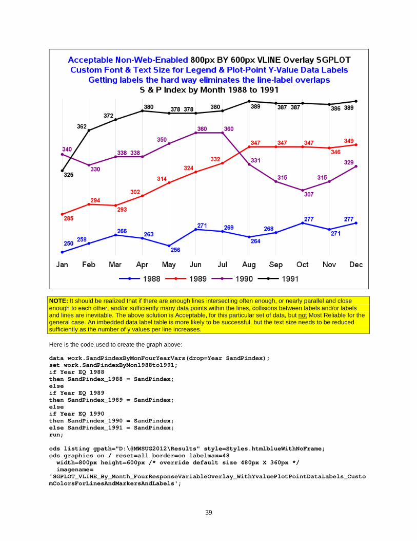
When experimenting with the TRANSPARENCY option that is available on the VLINE statement, which documentation says will lighten the lines and markers, I found that the data label text was also lightened to the same degree, thus preserving impaired readability. Good News: If you do some extra work with preprocessing the data and do some extra coding in the SGPLOT PROC step, it IS possible to remove the line-label overlaps, as is shown on the next page. What is surprising about the solution is that it also uses PROC SGPLOT and the VLINE statement, but the VLINE DATALABEL option delivers line-label collisions if you create the four lines using one VLINE statement with the GROUP=Year option, but no collisions if the lines are created with four separate, more complicated, VLINE statements with no GROUP option.

39

NOTE: It should be realized that if there are enough lines intersecting often enough, or nearly parallel and close enough to each other, and/or sufficiently many data points within the lines, collisions between labels and/or labels and lines are inevitable. The above solution is Acceptable, for this particular set of data, but not Most Reliable for the general case. An imbedded data label table is more likely to be successful, but the text size needs to be reduced sufficiently as the number of y values per line increases. Here is the code used to create the graph above: data work.SandPindexByMonFourYearVars(drop=Year SandPindex); set work.SandPindexByMon1988to1991; if Year EQ 1988 then SandPindex_1988 = SandPindex; else if Year EQ 1989 then SandPindex_1989 = SandPindex; else if Year EQ 1990 then SandPindex_1990 = SandPindex; else SandPindex_1991 = SandPindex; run; ods listing gpath="D:\@MWSUG2012\Results" style=Styles.htmlblueWithNoFrame; ods graphics on / reset=all border=on labelmax=48 width=800px height=600px /* override default size 480px X 360px */ imagename= 'SGPLOT_VLINE_By_Month_FourResponseVariableOverlay_WithYvaluePlotPointDataLabels_CustomColorsForLinesAndMarkersAndLabels';

40

title1 FONT='Albany AMT/Bold' HEIGHT=14 PT COLOR=Blue 'Acceptable Non-Web-Enabled ' COLOR=Black '800px BY 600px VLINE Overlay SGPLOT'; title2 FONT='Albany AMT/Bold' HEIGHT=14 PT COLOR=Blue 'Custom Font & Text Size for Legend & Plot-Point Y-Value Data Labels'; title3 FONT='Albany AMT/Bold' HEIGHT=14 PT COLOR=Blue 'Getting labels the hard way eliminates the line-label overlaps'; title4 FONT='Albany AMT/Bold' HEIGHT=14 PT 'S & P Index by Month 1988 to 1991'; proc sgplot data=work.SandPindexByMonFourYearVars; vline Month / response=SandPindex_1988 nostatlabel legendlabel='1988' markers markerattrs=(size=7 symbol=circlefilled color=blue) lineattrs=(thickness=3 pattern=solid color=blue) datalabel=SandPindex_1988 datalabelattrs=(family='Albany AMT/Bold' size=10 PT weight=Bold color=blue); vline Month / response=SandPindex_1989 nostatlabel legendlabel='1989' markers markerattrs=(size=7 symbol=circlefilled color=red) lineattrs=(thickness=3 pattern=solid color=red) datalabel=SandPindex_1989 datalabelattrs=(family='Albany AMT/Bold' size=10 PT weight=Bold color=red); vline Month / response=SandPindex_1990 nostatlabel legendlabel='1990' markers markerattrs=(size=7 symbol=circlefilled color=purple) lineattrs=(thickness=3 pattern=solid color=purple) datalabel=SandPindex_1990 datalabelattrs=(family='Albany AMT/Bold' size=10 PT weight=Bold color=purple); vline Month / response=SandPindex_1991 nostatlabel legendlabel='1991' markers markerattrs=(size=7 symbol=circlefilled color=black) lineattrs=(thickness=3 pattern=solid color=black) datalabel=SandPindex_1991 datalabelattrs=(family='Albany AMT/Bold' size=10 PT weight=Bold color=black); keylegend / noborder titleattrs=(family='Albany AMT/Bold' size=12 PT) valueattrs=(family='Albany AMT/Bold' size=12 PT); yaxis display=none; xaxis display=(nolabel noticks noline) grid valueattrs=(family='Albany AMT/Bold' size=12 PT) values=(1 to 12 by 1); format Month MonthAbbrev.; format SandPindex_1988 SandPindex_1989 SandPindex_1990 SandPindex_1991 5.; run; ods listing close; ods listing; The above code is more complex. In principle, one could convert it to a macro. It would be straightforward, but a lot of code. I leave it as an exercise for the interested and motivated reader, and would be grateful for a copy of the code. As a next step, let’s see what happens if one simply adds “datalabelpos=bottom” to each of the VLINE statements above, changes the graph titles and filename, provides LABEL statements for each response variable: label SandPindex_1988='1988'; label SandPindex_1989='1989'; label SandPindex_1990='1990'; label SandPindex_1991='1991'; and restores the y axis tick mark values by replacing yaxis display=none; with this statement yaxis display=(nolabel noticks noline) grid offsetmin=0.05 valueattrs=(family='Albany AMT/Bold' size=12 PT); The result is on the next page.

41

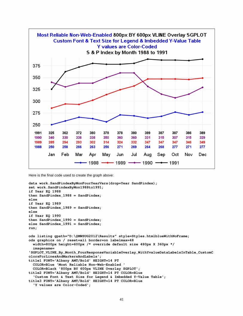
Here is the final code used to create the graph above: data work.SandPindexByMonFourYearVars(drop=Year SandPindex); set work.SandPindexByMon1988to1991; if Year EQ 1988 then SandPindex_1988 = SandPindex; else if Year EQ 1989 then SandPindex_1989 = SandPindex; else if Year EQ 1990 then SandPindex_1990 = SandPindex; else SandPindex_1991 = SandPindex; run; ods listing gpath="D:\@MWSUG2012\Results" style=Styles.htmlblueWithNoFrame; ods graphics on / reset=all border=on labelmax=48 width=800px height=600px /* override default size 480px X 360px */ imagename= 'SGPLOT_VLINE_By_Month_FourResponseVariableOverlay_WithYvalueDataLabelsInTable_CustomColorsForLinesAndMarkersAndLabels'; title1 FONT='Albany AMT/Bold' HEIGHT=14 PT COLOR=Blue 'Most Reliable Non-Web-Enabled ' COLOR=Black '800px BY 600px VLINE Overlay SGPLOT'; title2 FONT='Albany AMT/Bold' HEIGHT=14 PT COLOR=Blue 'Custom Font & Text Size for Legend & Imbedded Y-Value Table'; title3 FONT='Albany AMT/Bold' HEIGHT=14 PT COLOR=Blue 'Y values are Color-Coded';

42

title4 FONT='Albany AMT/Bold' HEIGHT=14 PT 'S & P Index by Month 1988 to 1991'; proc sgplot data=work.SandPindexByMonFourYearVars; vline Month / response=SandPindex_1988 nostatlabel legendlabel='1988' markers markerattrs=(size=7 symbol=circlefilled color=blue) lineattrs=(thickness=3 pattern=solid color=blue) datalabel=SandPindex_1988 datalabelattrs=(family='Albany AMT/Bold' size=10 PT weight=Bold color=blue) datalabelpos=bottom; vline Month / response=SandPindex_1989 nostatlabel legendlabel='1989' markers markerattrs=(size=7 symbol=circlefilled color=red) lineattrs=(thickness=3 pattern=solid color=red) datalabel=SandPindex_1989 datalabelattrs=(family='Albany AMT/Bold' size=10 PT weight=Bold color=red) datalabelpos=bottom; vline Month / response=SandPindex_1990 nostatlabel legendlabel='1990' markers markerattrs=(size=7 symbol=circlefilled color=purple) lineattrs=(thickness=3 pattern=solid color=purple) datalabel=SandPindex_1990 datalabelattrs=(family='Albany AMT/Bold' size=10 PT weight=Bold color=purple) datalabelpos=bottom; vline Month / response=SandPindex_1991 nostatlabel legendlabel='1991' markers markerattrs=(size=7 symbol=circlefilled color=black) lineattrs=(thickness=3 pattern=solid color=black) datalabel=SandPindex_1991 datalabelattrs=(family='Albany AMT/Bold' size=10 PT weight=Bold color=black) datalabelpos=bottom; keylegend / noborder titleattrs=(family='Albany AMT/Bold' size=12 PT) valueattrs=(family='Albany AMT/Bold' size=12 PT); yaxis display=(nolabel noticks noline) grid offsetmin=0.05 /* space between top of datalabel table & bottom of plot area */ valueattrs=(family='Albany AMT/Bold' size=12 PT); xaxis display=(nolabel noticks noline) grid valueattrs=(family='Albany AMT/Bold' size=12 PT) values=(1 to 12 by 1); format Month MonthAbbrev.; format SandPindex_1988 SandPindex_1989 SandPindex_1990 SandPindex_1991 5.; label SandPindex_1988='1988'; label SandPindex_1989='1989'; label SandPindex_1990='1990'; label SandPindex_1991='1991'; run; ods listing close; ods listing; As was the case for the improved solution for y-value plot-point data labels, the above code is complex. In principle, one could convert it to a macro. It would be straightforward, but a lot of code. I leave it as an exercise for the interested and motivated reader, and would be grateful for a copy of the code. My quest for a way to create a multi-line plot with an imbedded color-coded y-value table was inspired by seeing Philip R. Holland’s black-and-white multi-line plot with imbedded table, which relies on use of Graph Template Language (GTL) and PROC SGRENDER. See Reference 9.

43

GRAPH MACRO TOOLS YOU CAN USE IN SAS V9.3 My quest since 1981 for communication-effective graphs has yielded solutions that require extra coding. Macros can do that coding work for you, and give you simple parameters to specify instead, similar to using a SAS procedure. In this section, I share and show how to use three such macros for common uses with high-value results. Two of the macros overcome limitations in the new ODS GRAPHICS and SG procedures which are now an alternative to SAS/GRAPH. With those macros you need not use SAS/GRAPH to compensate for what is missing in the new technology. Their output charts are written to disk to later be inserted into Microsoft PowerPoint, Word, or Excel, or simply printed, but they could be web-enabled and packaged with ODS HTML. The third macro does create web-enabled output. However, its image file can be manually inserted into Microsoft PowerPoint, Word, or Excel, or simply printed. The macros require Version 9.3 of Base SAS software. The macros in this paper are suitable for management reporting in business, government, or other organizational settings, not statistical or heavy-duty analytical graphs. Although the SG (Statistical Graphics) procedures were originally developed for statistical graphics, they can be used for management reporting. By graphs for management reporting I mean graphs or web graphs used to answer common questions. E.g., how do measurements for different entities compare? This question is commonly answered visually with bar charts or pie charts. All of the macros provided here are in pursuit of visual communication effectiveness. Earlier in this paper, non-macro graphic solutions were provided that use ODS GRAPHICS and SG procedures. Two of those solutions are made easier and less error vulnerable by use of macros provided below. The third macro presented here creates one of the most powerful tools for efficient and effective comparison and impact assessment. The macro code is lengthy and complex, but once you have copied it out of here and filed it in a macro library, its use is easy and quick. Sample invocations of the macro are used here to create output examples. You do not need to read any of macro source code provided here. If you do, obviously you can use it as a starting point to create a derivative or alternative that you like better. Still in development by me for the third macro is a version that will have added capabilities that I supported in a SAS/GRAPH version for a production application. How To Use the Macros Copy the code for each macro into NotePad, save the result with filetype sas in any folder location convenient to you where you have write access as well as read access. The filename that you use must match the string after the %MACRO prefix in the first line of the macro. To run the macros, you must, as shown in the macro invocation example code, precede the macro invocation with this statement: OPTIONS SASAUTOS=( ThePathToYourFolderGoesHere SASAUTOS); An example of ThePathToYourFolderGoesHere could be:

"C:\MySASmacros" When you submit code to run the macro, SAS will first look for it in your folder, and then it will look for it in your default macro library location, which has path reference SASAUTOS. For every macro that is invoked during your session or in your batch program execution, until you override the above OPTIONS statement, SAS will always look in your macro library first.

44

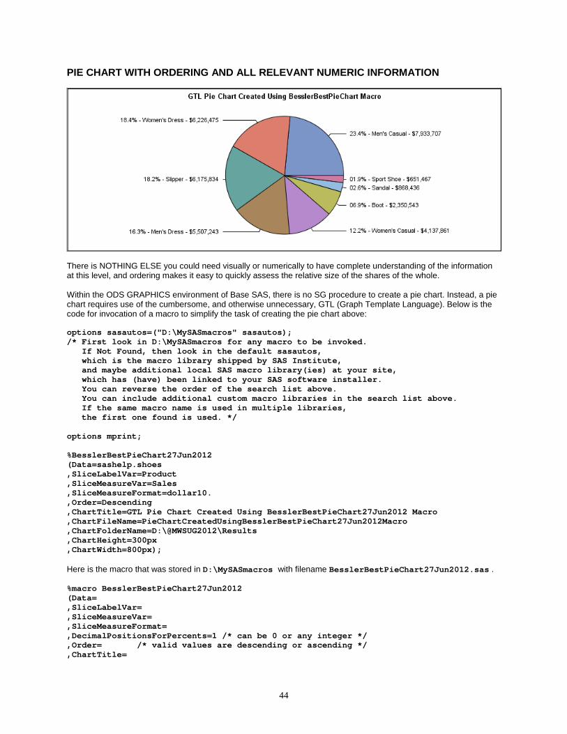
PIE CHART WITH ORDERING AND ALL RELEVANT NUMERIC INFORMATION

There is NOTHING ELSE you could need visually or numerically to have complete understanding of the information at this level, and ordering makes it easy to quickly assess the relative size of the shares of the whole. Within the ODS GRAPHICS environment of Base SAS, there is no SG procedure to create a pie chart. Instead, a pie chart requires use of the cumbersome, and otherwise unnecessary, GTL (Graph Template Language). Below is the code for invocation of a macro to simplify the task of creating the pie chart above: options sasautos=("D:\MySASmacros" sasautos); /* First look in D:\MySASmacros for any macro to be invoked. If Not Found, then look in the default sasautos, which is the macro library shipped by SAS Institute, and maybe additional local SAS macro library(ies) at your site, which has (have) been linked to your SAS software installer. You can reverse the order of the search list above. You can include additional custom macro libraries in the search list above. If the same macro name is used in multiple libraries, the first one found is used. */ options mprint; %BesslerBestPieChart27Jun2012 (Data=sashelp.shoes ,SliceLabelVar=Product ,SliceMeasureVar=Sales ,SliceMeasureFormat=dollar10. ,Order=Descending ,ChartTitle=GTL Pie Chart Created Using BesslerBestPieChart27Jun2012 Macro ,ChartFileName=PieChartCreatedUsingBesslerBestPieChart27Jun2012Macro ,ChartFolderName=D:\@MWSUG2012\Results ,ChartHeight=300px ,ChartWidth=800px); Here is the macro that was stored in D:\MySASmacros with filename BesslerBestPieChart27Jun2012.sas . %macro BesslerBestPieChart27Jun2012 (Data= ,SliceLabelVar= ,SliceMeasureVar= ,SliceMeasureFormat= ,DecimalPositionsForPercents=1 /* can be 0 or any integer */ ,Order= /* valid values are descending or ascending */ ,ChartTitle=

45

,ChartFileName= ,ChartFolderName= ,ChartHeight= ,ChartWidth= ); * All parameters above, except Order are mandatory *; * If Order is not specified, the SAS PROC SORT default is ascending *; proc summary data=&Data nway; class &SliceLabelVar; var &SliceMeasureVar; output out=ToPrep sum=TotalByClass; run; proc sql noprint; select sum(TotalByClass) into :GrandTotal from ToPrep; quit; data ToChart; length SliceNameWithPercentAndValue $ 256; /* over-sized, but that is harmless */ set ToPrep; SliceNameWithPercentAndValue = trim(left( put(((TotalByClass / &GrandTotal) * 100),z4.&DecimalPositionsForPercents) )) || '% - ' || trim(left(&SliceLabelVar)) || ' - ' || trim(left(put(TotalByClass,&SliceMeasureFormat))); run; proc sort data=ToChart; by &Order TotalByClass; run; proc template; define statgraph BesslerBestPieChart27Jun2012; begingraph; entrytitle "&ChartTitle"; layout region; piechart category=SliceNameWithPercentAndValue response=TotalByClass / datalabelcontent=(category) datalabellocation=callout otherslice=FALSE; endlayout; endgraph; end; run; ods listing gpath="&ChartFolderName"; ods graphics on / reset=all border=on height=&ChartHeight width=&ChartWidth imagename="&ChartFileName"; proc sgrender data=ToChart template=BesslerBestPieChart27Jun2012; run; ods listing close; ods listing; %mend BesslerBestPieChart27Jun2012;

46

BAR CHART OF SUMS WITH PERCENT SHARES: ALTERNATIVE FOR WHEN PIE CHART IS INFEASIBLE OR UNACCEPTABLE I have long been an advocate for horizontal bar charts rather than vertical bar charts. Vertical bar charts work well only when the bar labels are short. Tilted, or worse, vertical labels for vertical bars are somewhere between inelegant and outright anti-communicative. With V9.2, the length on labels was extended to 256, which is always adequate, and, for horizontal bar charts, always useful for longer labels that are, in fact, often needed. 256 would be impractical (no space left for the bar—unless you expand the image width, which IS possible), but it’s a welcome, friendly limit.

Just as the pie chart labels included values, not just slice names and percent shares, bar chart labels created in this macro COULD include values also, and the values at bar ends could be dropped. I leave that macro enhancement to the reader. See the code for the last macro in this paper for another way to compose multi-function bar chart labels. The main advantage of SGPLOT bar charts is that you can get the values at the bar ends with no extraordinary effort. A PROC GCHART bar chart by default places those values in a stack or table at the right margin of the graph area. To get them at the bar ends requires use of the ANNOTATE facility, which is more work—best avoided if possible. Below is the code for invocation of a macro to simplify the task of creating the bar chart above: options sasautos=("D:\MySASmacros" sasautos); /* First look in D:\MySASmacros for any macro to be invoked. If Not Found, then look in the default sasautos, which is the macro library shipped by SAS Institute, and maybe additional local SAS macro library(ies) at your site, which has (have) been linked to your SAS software installer. You can reverse the order of the search list above. You can include additional custom macro libraries in the search list above. If the same macro name is used in multiple libraries, the first one found is used. */ options mprint; %HBARsummaryChartWithPctShares (Data=sashelp.shoes ,BarLabelVar=Product ,BarMeasureVar=Sales ,FontSize=16pt ,BarWidth=0.5 ,Order=Descending ,ChartTitle=Horizontal Bar Chart of Ranked Totals and Percent Shares Using HBARsummaryChartWithPctShares Macro ,ChartFileName=BarChartCreatedUsingHBARsummaryChartWithPctSharesMacro ,ChartFolderName=D:\@MWSUG2012\Results ,ChartHeight=303px /* NOTE: At 300px, every other bar label is omitted by SAS. */ ,ChartWidth=800px); /* See discussion of FitPolicy=THIN earlier in this paper. */

47

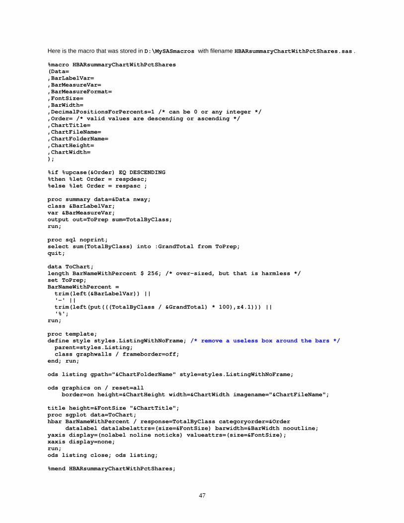
Here is the macro that was stored in D:\MySASmacros with filename HBARsummaryChartWithPctShares.sas . %macro HBARsummaryChartWithPctShares (Data= ,BarLabelVar= ,BarMeasureVar= ,BarMeasureFormat= ,FontSize= ,BarWidth= ,DecimalPositionsForPercents=1 /* can be 0 or any integer */ ,Order= /* valid values are descending or ascending */ ,ChartTitle= ,ChartFileName= ,ChartFolderName= ,ChartHeight= ,ChartWidth= ); %if %upcase(&Order) EQ DESCENDING %then %let Order = respdesc; %else %let Order = respasc ; proc summary data=&Data nway; class &BarLabelVar; var &BarMeasureVar; output out=ToPrep sum=TotalByClass; run; proc sql noprint; select sum(TotalByClass) into :GrandTotal from ToPrep; quit; data ToChart; length BarNameWithPercent $ 256; /* over-sized, but that is harmless */ set ToPrep; BarNameWithPercent = trim(left(&BarLabelVar)) || '-' || trim(left(put(((TotalByClass / &GrandTotal) * 100),z4.1))) || '%'; run; proc template; define style styles.ListingWithNoFrame; /* remove a useless box around the bars */ parent=styles.Listing; class graphwalls / frameborder=off; end; run; ods listing gpath="&ChartFolderName" style=styles.ListingWithNoFrame; ods graphics on / reset=all border=on height=&ChartHeight width=&ChartWidth imagename="&ChartFileName"; title height=&FontSize "&ChartTitle"; proc sgplot data=ToChart; hbar BarNameWithPercent / response=TotalByClass categoryorder=&Order datalabel datalabelattrs=(size=&FontSize) barwidth=&BarWidth nooutline; yaxis display=(nolabel noline noticks) valueattrs=(size=&FontSize); xaxis display=none; run; ods listing close; ods listing; %mend HBARsummaryChartWithPctShares;

48

SOLUTIONS FOR A FINITE WORK DAY IN AN ERA OF INFORMATION OVERLOAD: HOW THEM WHAT IS IMPORTANT . . . WITH THE SUBSETTED AND RANKED HORIZONTAL BAR CHART For over a quarter century I have advocated and exploited use of the subsetted and ranked horizontal bar chart. I have long been hooked on the idea of trying to deliver only the most important. The most important can usually fit on one sheet of paper, and frequently, if not almost always, on one web page without having to scroll. Such limitation of information volume reminds me of the wisdom of Kenneth J. Wesley, my staff who once counseled me, when I was agonizing over a report for executive management, that “If it doesn’t fit on one page, they won’t read it.” And I always remember the wisdom of Jim White, an expert on print document design, who said, “Let part stand for the whole.” In that spirit, I developed a macro that allowed the user to point to a data set and create a bar chart subsetted in any one of three ways: (1) Top N (where N was any integer); (2) all values above a cut-off; or (3) enough of the top values to account for the Top P Percent of the total measure of interest. Whereas I have long maintained that what will fit on a page, say, anywhere from the Top 10 to the Top 40 or 50, will usually account for 80 to sometimes 99% of the total measure of interest, a reliable approach to take when subsetting is to stop reporting as soon as the chart bars account for as much of the total as you feel is important to show. YOU pick the percent target with Option 3 above. Recently, I decided I wanted a client’s reporting system users to be able to optionally look at the WHOLE list. The macro that I am sharing here does NOT support that four-option capability. What was delivered for the client was actually a macro that not only created four versions of the ranking report, but also interlinked the four web graphs with hyperlinks—very cool and maximally convenient. Here I provide a more limited function macro that successfully sizes the height of the image file for ANY number of the Top N bars up to a maximum of 50 and links it forwards and backwards with an image sized large enough to display ALL of the bars. Of course, if you do not really want the ALL-bars companion chart, it is easy to modify the macro to omit that capability. (I could have built in the option, but the macro is complicated enough As Is.) If the Top N number of bars requested is not less than the total number of bars possible, only one web page is produced. For this macro to perform reliably regardless of the number of Top N bars (up to 50), the SGPLOT HBAR chart image file must be sufficiently tall and/or the font used for bar labels must be significantly small to avoid automatic thinning of the bar labels. (See the earlier discussion in this paper of thinning tick mark values in line plots.) At the same time, the image file must be sufficiently small to fit in the browser window so that all of the Top N bars can be viewed without need for vertical scrolling. (The ALL Bars chart will require scrolling unless ALL is less than 51.) So, there is a trade-off between: (a) making the bar label font small enough so that the desired number of Top N bars will not experience thinning; (b) making the bar label font small enough to that the Top N bar chart will not require vertical scrolling; and (c) making the bar label font large enough to be easily readable. The viewing capacity of the expected target user depends on the brand and version number of the web browser, how many toolbars are in use in the web browser, and the vertical resolution of the monitor. My development and testing of the examples shown here were done using a monitor with 1920 X 1080 resolution, Internet Explorer Version 9, and no (what I regard as) extra toolbars. The default font, which can be overridden by the macro user, is Albany AMT/Bold. This font is shipped with SAS software. The font size used by the macro is controlled internally, and varies by the value of TopN. The algorithm in the macro that controls font size also determines the appropriate number of Y pixels per bar based on the value of TopN. There is an overhead number of Y pixels which is independent of the value of TopN. The overhead is a macro parameter defaulted to what I found appropriate for the default choice of bar label font. The macro dynamically determines the total number of Y pixels needed. Macro internals must be revised if using a different font for the bar labels. It required experimentation and testing to determine the relationship between TopN, font size, Y pixels per bar, and Y pixels overhead—in pursuit of preventing the dreaded automatic thinning of bar labels. The macro default font size for the title lines is 16 pt. Reducing it might facilitate fitting your chart in browser window on a lower resolution monitor. The title lines are OUTSIDE of and above the image file. To save vertical space, you can avoid use of the optional fifth title line. That line can be used for optional diagnostic information during testing. When not testing, you can optionally provide any text, with any color of your choice (default is black). Without or without such optional text, you can include (only in black) the run day, date, and time on title line 5. NOTE: I later provide a non-web/non-HTML version of the macro, which can create an image file on disk to be imbedded manually in Microsoft Word or Microsoft PowerPoint, and perfectly sized for whichever use you need.

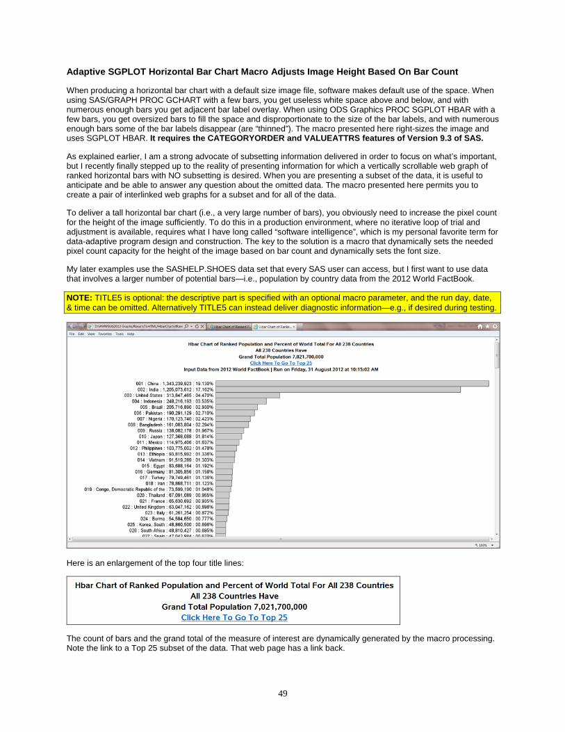
49

Adaptive SGPLOT Horizontal Bar Chart Macro Adjusts Image Height Based On Bar Count When producing a horizontal bar chart with a default size image file, software makes default use of the space. When using SAS/GRAPH PROC GCHART with a few bars, you get useless white space above and below, and with numerous enough bars you get adjacent bar label overlay. When using ODS Graphics PROC SGPLOT HBAR with a few bars, you get oversized bars to fill the space and disproportionate to the size of the bar labels, and with numerous enough bars some of the bar labels disappear (are “thinned”). The macro presented here right-sizes the image and uses SGPLOT HBAR. It requires the CATEGORYORDER and VALUEATTRS features of Version 9.3 of SAS. As explained earlier, I am a strong advocate of subsetting information delivered in order to focus on what’s important, but I recently finally stepped up to the reality of presenting information for which a vertically scrollable web graph of ranked horizontal bars with NO subsetting is desired. When you are presenting a subset of the data, it is useful to anticipate and be able to answer any question about the omitted data. The macro presented here permits you to create a pair of interlinked web graphs for a subset and for all of the data. To deliver a tall horizontal bar chart (i.e., a very large number of bars), you obviously need to increase the pixel count for the height of the image sufficiently. To do this in a production environment, where no iterative loop of trial and adjustment is available, requires what I have long called “software intelligence”, which is my personal favorite term for data-adaptive program design and construction. The key to the solution is a macro that dynamically sets the needed pixel count capacity for the height of the image based on bar count and dynamically sets the font size. My later examples use the SASHELP.SHOES data set that every SAS user can access, but I first want to use data that involves a larger number of potential bars—i.e., population by country data from the 2012 World FactBook. NOTE: TITLE5 is optional: the descriptive part is specified with an optional macro parameter, and the run day, date, & time can be omitted. Alternatively TITLE5 can instead deliver diagnostic information—e.g., if desired during testing.

Here is an enlargement of the top four title lines:

The count of bars and the grand total of the measure of interest are dynamically generated by the macro processing. Note the link to a Top 25 subset of the data. That web page has a link back.

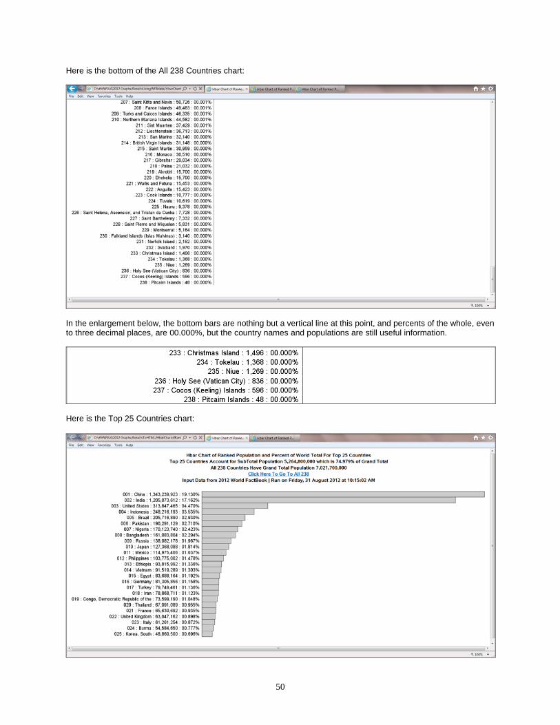
50

Here is the bottom of the All 238 Countries chart:

In the enlargement below, the bottom bars are nothing but a vertical line at this point, and percents of the whole, even to three decimal places, are 00.000%, but the country names and populations are still useful information.

Here is the Top 25 Countries chart:

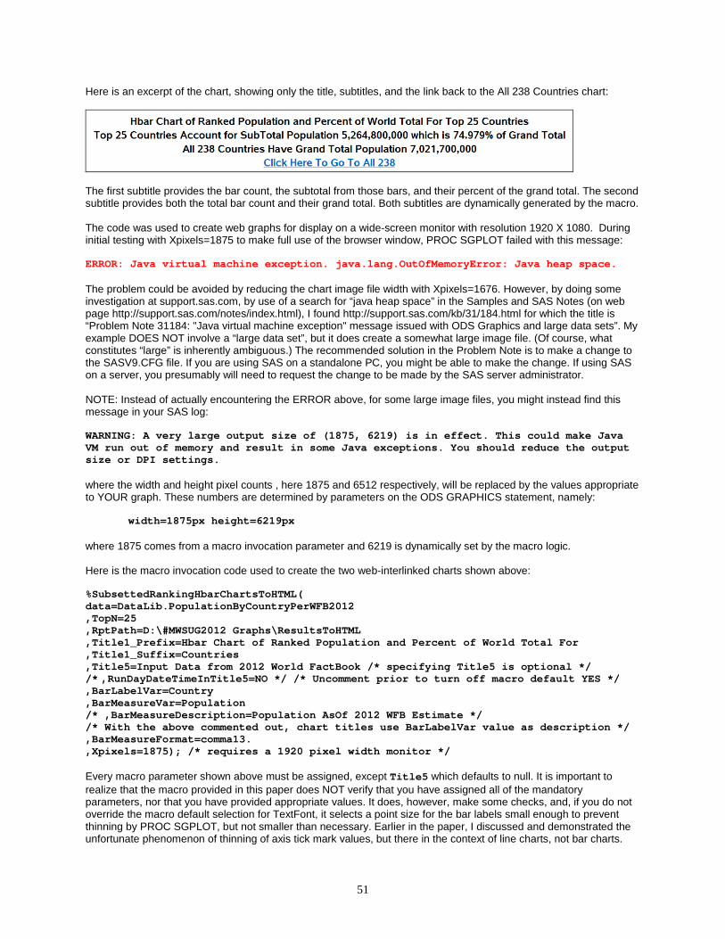
51

Here is an excerpt of the chart, showing only the title, subtitles, and the link back to the All 238 Countries chart:

The first subtitle provides the bar count, the subtotal from those bars, and their percent of the grand total. The second subtitle provides both the total bar count and their grand total. Both subtitles are dynamically generated by the macro. The code was used to create web graphs for display on a wide-screen monitor with resolution 1920 X 1080. During initial testing with Xpixels=1875 to make full use of the browser window, PROC SGPLOT failed with this message: ERROR: Java virtual machine exception. java.lang.OutOfMemoryError: Java heap space. The problem could be avoided by reducing the chart image file width with Xpixels=1676. However, by doing some investigation at support.sas.com, by use of a search for “java heap space” in the Samples and SAS Notes (on web page http://support.sas.com/notes/index.html), I found http://support.sas.com/kb/31/184.html for which the title is “Problem Note 31184: "Java virtual machine exception" message issued with ODS Graphics and large data sets”. My example DOES NOT involve a “large data set”, but it does create a somewhat large image file. (Of course, what constitutes “large” is inherently ambiguous.) The recommended solution in the Problem Note is to make a change to the SASV9.CFG file. If you are using SAS on a standalone PC, you might be able to make the change. If using SAS on a server, you presumably will need to request the change to be made by the SAS server administrator. NOTE: Instead of actually encountering the ERROR above, for some large image files, you might instead find this message in your SAS log: WARNING: A very large output size of (1875, 6219) is in effect. This could make Java VM run out of memory and result in some Java exceptions. You should reduce the output size or DPI settings. where the width and height pixel counts , here 1875 and 6512 respectively, will be replaced by the values appropriate to YOUR graph. These numbers are determined by parameters on the ODS GRAPHICS statement, namely:

width=1875px height=6219px where 1875 comes from a macro invocation parameter and 6219 is dynamically set by the macro logic. Here is the macro invocation code used to create the two web-interlinked charts shown above: %SubsettedRankingHbarChartsToHTML( data=DataLib.PopulationByCountryPerWFB2012 ,TopN=25 ,RptPath=D:\#MWSUG2012 Graphs\ResultsToHTML ,Title1_Prefix=Hbar Chart of Ranked Population and Percent of World Total For ,Title1_Suffix=Countries ,Title5=Input Data from 2012 World FactBook /* specifying Title5 is optional */ /* ,RunDayDateTimeInTitle5=NO */ /* Uncomment prior to turn off macro default YES */ ,BarLabelVar=Country ,BarMeasureVar=Population /* ,BarMeasureDescription=Population AsOf 2012 WFB Estimate */ /* With the above commented out, chart titles use BarLabelVar value as description */ ,BarMeasureFormat=comma13. ,Xpixels=1875); /* requires a 1920 pixel width monitor */ Every macro parameter shown above must be assigned, except Title5 which defaults to null. It is important to realize that the macro provided in this paper does NOT verify that you have assigned all of the mandatory parameters, nor that you have provided appropriate values. It does, however, make some checks, and, if you do not override the macro default selection for TextFont, it selects a point size for the bar labels small enough to prevent thinning by PROC SGPLOT, but not smaller than necessary. Earlier in the paper, I discussed and demonstrated the unfortunate phenomenon of thinning of axis tick mark values, but there in the context of line charts, not bar charts.

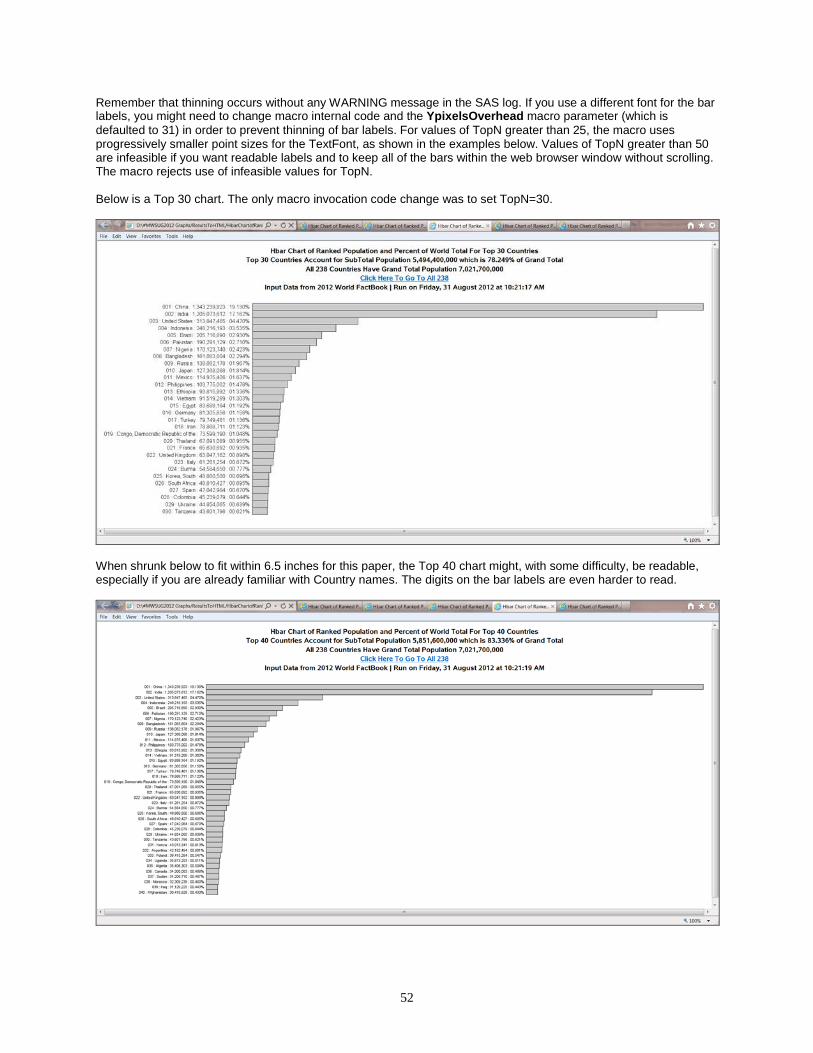
52

Remember that thinning occurs without any WARNING message in the SAS log. If you use a different font for the bar labels, you might need to change macro internal code and the YpixelsOverhead macro parameter (which is defaulted to 31) in order to prevent thinning of bar labels. For values of TopN greater than 25, the macro uses progressively smaller point sizes for the TextFont, as shown in the examples below. Values of TopN greater than 50 are infeasible if you want readable labels and to keep all of the bars within the web browser window without scrolling. The macro rejects use of infeasible values for TopN. Below is a Top 30 chart. The only macro invocation code change was to set TopN=30.

When shrunk below to fit within 6.5 inches for this paper, the Top 40 chart might, with some difficulty, be readable, especially if you are already familiar with Country names. The digits on the bar labels are even harder to read.

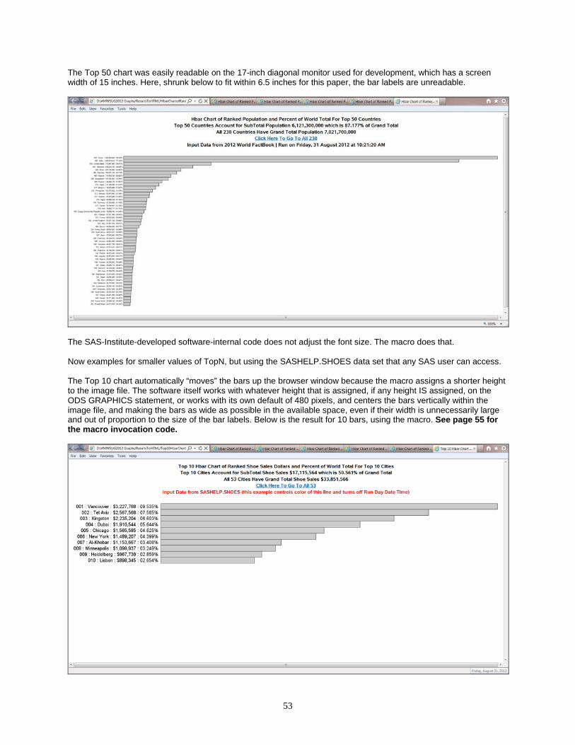
53

The Top 50 chart was easily readable on the 17-inch diagonal monitor used for development, which has a screen width of 15 inches. Here, shrunk below to fit within 6.5 inches for this paper, the bar labels are unreadable.

The SAS-Institute-developed software-internal code does not adjust the font size. The macro does that. Now examples for smaller values of TopN, but using the SASHELP.SHOES data set that any SAS user can access. The Top 10 chart automatically “moves” the bars up the browser window because the macro assigns a shorter height to the image file. The software itself works with whatever height that is assigned, if any height IS assigned, on the ODS GRAPHICS statement, or works with its own default of 480 pixels, and centers the bars vertically within the image file, and making the bars as wide as possible in the available space, even if their width is unnecessarily large and out of proportion to the size of the bar labels. Below is the result for 10 bars, using the macro. See page 55 for the macro invocation code.

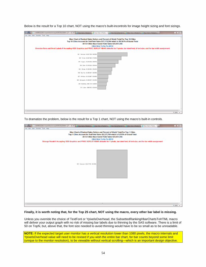
54

Below is the result for a Top 10 chart, NOT using the macro’s built-incontrols for image height sizing and font sizings.

To dramatize the problem, below is the result for a Top 1 chart, NOT using the macro’s built-in controls.

Finally, it is worth noting that, for the Top 25 chart, NOT using the macro, every other bar label is missing. Unless you override the choice of TextFont or YpixelsOverhead, the SubsettedRankingHbarChartsToHTML macro will deliver your output graph with no risk of missing bar labels due to thinning by the SAS software. There is a limit of 50 on TopN, but, above that, the font size needed to avoid thinning would have to be so small as to be unreadable. NOTE: If the expected target user monitor has a vertical resolution lower than 1080 pixels, the macro internals and YpixelsOverhead value will need to be revised if you wish the entire bar chart, for bar counts beyond some limit (unique to the monitor resolution), to be viewable without vertical scrolling—which is an important design objective.

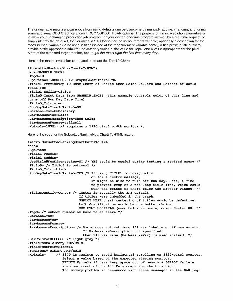
55

The undesirable results shown above from using defaults can be overcome by manually adding, changing, and tuning some additional ODS Graphics and/or PROC SGPLOT HBAR options. The purpose of a macro solution alternative is to allow your unchanging production job program, or your written-one-time program invoked by a real-time request, to simply identify the data set, the variables, a SAS format for the measurement variable, optionally a description for the measurement variable (to be used in titles instead of the measurement variable name), a title prefix, a title suffix to provide a title-appropriate label for the category variable, the value for TopN, and a value appropriate for the pixel width of the expected target monitor, and to get the result right the first time every time. Here is the macro invocation code used to create the Top 10 Chart: %SubsettedRankingHbarChartsToHTML( data=SASHELP.SHOES ,TopN=10 ,RptPath=D:\#MWSUG2012 Graphs\ResultsToHTML ,Title1_Prefix=Top 10 Hbar Chart of Ranked Shoe Sales Dollars and Percent of World Total For ,Title1_Suffix=Cities ,Title5=Input Data from SASHELP.SHOES (this example controls color of this line and turns off Run Day Date Time) ,Title5_Color=red ,RunDayDateTimeInTitle5=NO ,BarLabelVar=Subsidiary ,BarMeasureVar=Sales ,BarMeasureDescription=Shoe Sales ,BarMeasureFormat=dollar11. ,Xpixels=1875); /* requires a 1920 pixel width monitor */ Here is the code for the SubsettedRankingHbarChartsToHTML macro: %macro SubsettedRankingHbarChartsToHTML( data= ,RptPath= ,Title1_Prefix= ,Title1_Suffix= ,UseTitle5ForDiagnostics=NO /* YES could be useful during testing a revised macro */ ,Title5= /* Title5 is optional */ ,Title5_Color=black ,RunDayDateTimeInTitle5=YES /* If using TITLE5 for diagnostic or for a custom message, it might be wise to turn off Run Day, Date, & Time to prevent wrap of a too long title line, which could push the bottom of chart below the browser window. */ ,TitlesJustify=Center /* Center is actually the SAS default. If titles were imbedded in the graph, SGPLOT HBAR chart centering of titles would be defective. Left Justification would be the better choice. ODS HTML NOGTITLE (used below in macro) makes Center OK. */ ,TopN= /* subset number of bars to be shown */ ,BarLabelVar= ,BarMeasureVar= ,BarMeasureFormat= ,BarMeasureDescription= /* Macro does not retrieve SAS var label even if one exists. If BarMeasureDescription not specified, then SAS var name (BarMeasureVar) is used instead. */ ,BarColor=CXCCCCCC /* light grey */ ,TitleFont='Albany AMT/Bold' ,TitleFontPointSize=16 ,TextFont='Albany AMT/Bold' ,Xpixels= /* 1875 is maximum to avoid horizontal scrolling on 1920-pixel monitor. Select a value based on the expected viewing monitor. REDUCE Xpixels if java heap space out of memory & SGPLOT failure when bar count of the All Bars companion chart is high. The memory problem is announced with these messages in the SAS log:

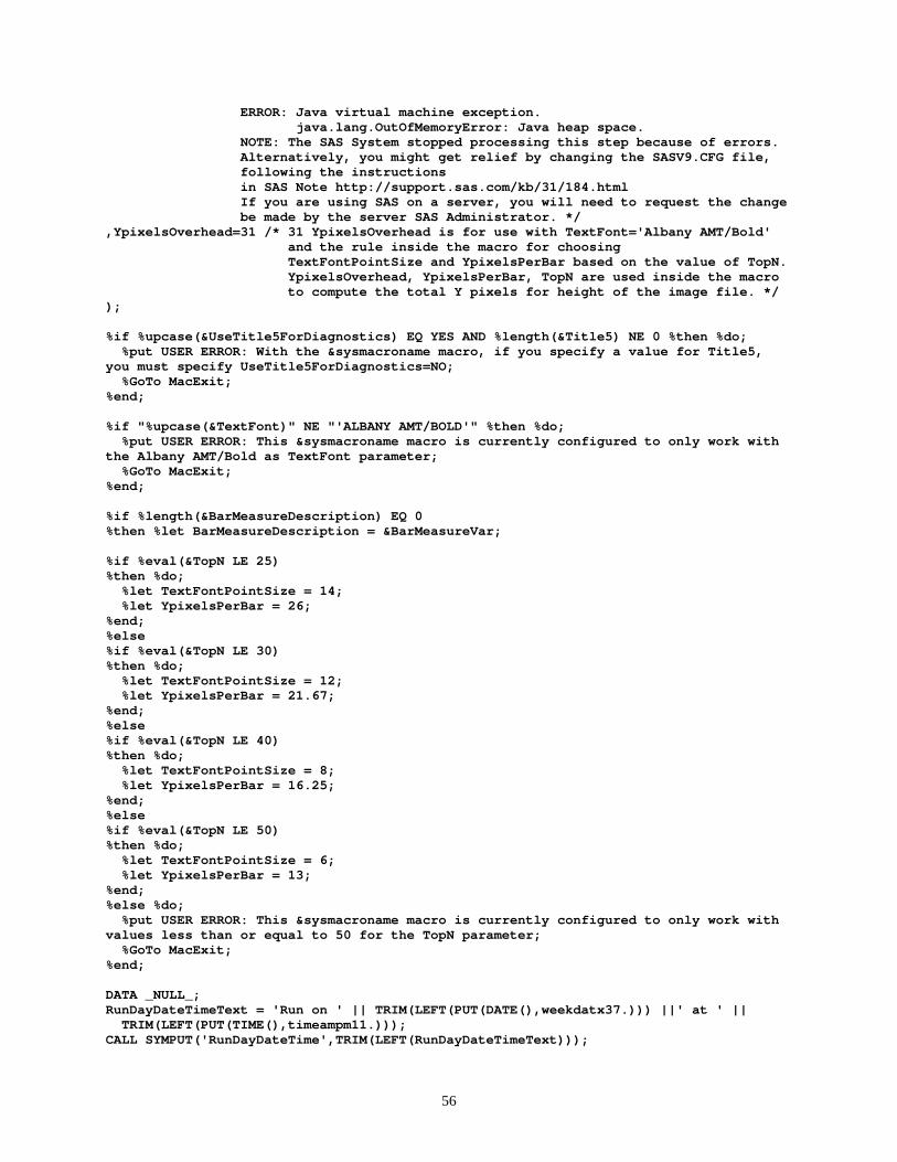
56

ERROR: Java virtual machine exception. java.lang.OutOfMemoryError: Java heap space. NOTE: The SAS System stopped processing this step because of errors. Alternatively, you might get relief by changing the SASV9.CFG file, following the instructions in SAS Note http://support.sas.com/kb/31/184.html If you are using SAS on a server, you will need to request the change be made by the server SAS Administrator. */ ,YpixelsOverhead=31 /* 31 YpixelsOverhead is for use with TextFont='Albany AMT/Bold' and the rule inside the macro for choosing TextFontPointSize and YpixelsPerBar based on the value of TopN. YpixelsOverhead, YpixelsPerBar, TopN are used inside the macro to compute the total Y pixels for height of the image file. */ ); %if %upcase(&UseTitle5ForDiagnostics) EQ YES AND %length(&Title5) NE 0 %then %do; %put USER ERROR: With the &sysmacroname macro, if you specify a value for Title5, you must specify UseTitle5ForDiagnostics=NO; %GoTo MacExit; %end; %if "%upcase(&TextFont)" NE "'ALBANY AMT/BOLD'" %then %do; %put USER ERROR: This &sysmacroname macro is currently configured to only work with the Albany AMT/Bold as TextFont parameter; %GoTo MacExit; %end; %if %length(&BarMeasureDescription) EQ 0 %then %let BarMeasureDescription = &BarMeasureVar; %if %eval(&TopN LE 25) %then %do; %let TextFontPointSize = 14; %let YpixelsPerBar = 26; %end; %else %if %eval(&TopN LE 30) %then %do; %let TextFontPointSize = 12; %let YpixelsPerBar = 21.67; %end; %else %if %eval(&TopN LE 40) %then %do; %let TextFontPointSize = 8; %let YpixelsPerBar = 16.25; %end; %else %if %eval(&TopN LE 50) %then %do; %let TextFontPointSize = 6; %let YpixelsPerBar = 13; %end; %else %do; %put USER ERROR: This &sysmacroname macro is currently configured to only work with values less than or equal to 50 for the TopN parameter; %GoTo MacExit; %end; DATA _NULL_; RunDayDateTimeText = 'Run on ' || TRIM(LEFT(PUT(DATE(),weekdatx37.))) ||' at ' || TRIM(LEFT(PUT(TIME(),timeampm11.))); CALL SYMPUT('RunDayDateTime',TRIM(LEFT(RunDayDateTimeText)));

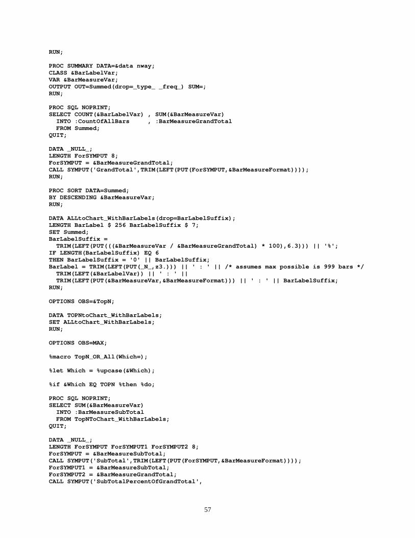
57

RUN; PROC SUMMARY DATA=&data nway; CLASS &BarLabelVar; VAR &BarMeasureVar; OUTPUT OUT=Summed(drop=_type_ _freq_) SUM=; RUN; PROC SQL NOPRINT; SELECT COUNT(&BarLabelVar) , SUM(&BarMeasureVar) INTO :CountOfAllBars , :BarMeasureGrandTotal FROM Summed; QUIT; DATA _NULL_; LENGTH ForSYMPUT 8; ForSYMPUT = &BarMeasureGrandTotal; CALL SYMPUT('GrandTotal',TRIM(LEFT(PUT(ForSYMPUT,&BarMeasureFormat)))); RUN; PROC SORT DATA=Summed; BY DESCENDING &BarMeasureVar; RUN; DATA ALLtoChart_WithBarLabels(drop=BarLabelSuffix); LENGTH BarLabel $ 256 BarLabelSuffix $ 7; SET Summed; BarLabelSuffix = TRIM(LEFT(PUT(((&BarMeasureVar / &BarMeasureGrandTotal) * 100),6.3))) || '%'; IF LENGTH(BarLabelSuffix) EQ 6 THEN BarLabelSuffix = '0' || BarLabelSuffix; BarLabel = TRIM(LEFT(PUT(_N_,z3.))) || ' : ' || /* assumes max possible is 999 bars */ TRIM(LEFT(&BarLabelVar)) || ' : ' || TRIM(LEFT(PUT(&BarMeasureVar,&BarMeasureFormat))) || ' : ' || BarLabelSuffix; RUN; OPTIONS OBS=&TopN; DATA TOPNtoChart_WithBarLabels; SET ALLtoChart_WithBarLabels; RUN; OPTIONS OBS=MAX; %macro TopN_OR_All(Which=); %let Which = %upcase(&Which); %if &Which EQ TOPN %then %do; PROC SQL NOPRINT; SELECT SUM(&BarMeasureVar) INTO :BarMeasureSubTotal FROM TopNToChart_WithBarLabels; QUIT; DATA _NULL_; LENGTH ForSYMPUT ForSYMPUT1 ForSYMPUT2 8; ForSYMPUT = &BarMeasureSubTotal; CALL SYMPUT('SubTotal',TRIM(LEFT(PUT(ForSYMPUT,&BarMeasureFormat)))); ForSYMPUT1 = &BarMeasureSubTotal; ForSYMPUT2 = &BarMeasureGrandTotal; CALL SYMPUT('SubTotalPercentOfGrandTotal',

58

TRIM(LEFT(PUT(( ForSYMPUT1 / ForSYMPUT2 ) * 100 , 6.3)))); RUN; %end; %if &Which EQ TOPN %then %let CountOfSelectedBars = &TopN; %else %let CountOfSelectedBars = &CountOfAllBars; %let Y_pixels = %eval( %sysfunc(CEIL( %sysevalf(&CountOfSelectedBars * &YpixelsPerBar) )) + &YpixelsOverhead ); %if &Which EQ ALL %then %do; %let Title1 = &Title1_Prefix.%str( All )&CountOfAllBars &Title1_Suffix; %let Title2 = All &CountOfAllBars &Title1_Suffix Have; %let Title3 = Grand Total &BarMeasureDescription &GrandTotal; %let Title4_LinkDescription = Top &TopN; %end; %else %do; %let Title1 = &Title1_Prefix.%str( Top )&TopN &Title1_Suffix; %let Title2 = Top &CountOfSelectedBars &Title1_Suffix Account for SubTotal &BarMeasureDescription &SubTotal which is &SubTotalPercentOfGrandTotal% of Grand Total; /* Because Title2 is delivered by HTML source code due to the specification of ODS HTML . . . NOGTITLE any extra blanks between the three parts of Title2 on three separate lines in the %LET statement above will be compressed down to one blank. */ %let Title3 = All &CountOfAllBars &Title1_Suffix Have Grand Total &BarMeasureDescription &GrandTotal; %let Title4_LinkDescription = All &CountOfAllBars; %end; %if %eval(&CountOfAllBars GT &TopN) %then %do; %let FileName_Temp = %sysfunc(COMPRESS(&Title1,' ')); %let FileNameLinkTo_Temp = %sysfunc(COMPRESS(&Title1_Prefix.&Title4_LinkDescription&Title1_Suffix)); %let FileName = &FileName_Temp._LinkedTo_&FileNameLinkTo_Temp; %let FileNameLinkTo = &FileNameLinkTo_Temp._LinkedTo_&FileName_Temp; %end; %else %let FileName = %sysfunc(COMPRESS(&Title1,' ')); %if &UseTitle5ForDiagnostics EQ YES %then %do; %let Title5ForDiagnostics = &CountOfSelectedBars bars, &YpixelsPerBar Ypixels per bar, &YpixelsOverhead Ypixels overhead, &Y_pixels Total Ypixels, &Xpixels Xpixels, Titles &TitleFontPointSize.pt &TitleFont, Bar Labels &TextFontPointSize.pt &TextFont; %let Title5ForDiagnostics = %sysfunc(compbl(%quote(&Title5ForDiagnostics))); %end; ODS GRAPHICS ON / RESET=ALL BORDER=OFF SCALE=OFF HEIGHT=&Y_pixels.px WIDTH=&Xpixels.px IMAGENAME="&FileName"; FOOTNOTE; ODS NORESULTS; ODS LISTING CLOSE;

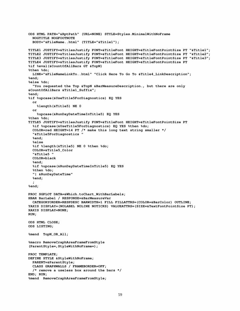
59

ODS HTML PATH="&RptPath" (URL=NONE) STYLE=Styles.MinimalWithNoFrame NOGTITLE NOGFOOTNOTE BODY="&FileName..html" (TITLE="&Title1"); TITLE1 JUSTIFY=&TitlesJustify FONT=&TitleFont HEIGHT=&TitleFontPointSize PT "&Title1"; TITLE2 JUSTIFY=&TitlesJustify FONT=&TitleFont HEIGHT=&TitleFontPointSize PT "&Title2"; TITLE3 JUSTIFY=&TitlesJustify FONT=&TitleFont HEIGHT=&TitleFontPointSize PT "&Title3"; TITLE4 JUSTIFY=&TitlesJustify FONT=&TitleFont HEIGHT=&TitleFontPointSize PT %if %eval(&CountOfAllBars GT &TopN) %then %do; LINK="&FileNameLinkTo..html" "Click Here To Go To &Title4_LinkDescription"; %end; %else %do; "You requested the Top &TopN &BarMeasureDescription., but there are only &CountOfAllBars &Title1_Suffix"; %end; %if %upcase(&UseTitle5ForDiagnostics) EQ YES or %length(&Title5) NE 0 or %upcase(&RunDayDateTimeInTitle5) EQ YES %then %do; TITLE5 JUSTIFY=&TitlesJustify FONT=&TitleFont HEIGHT=&TitleFontPointSize PT %if %upcase(&UseTitle5ForDiagnostics) EQ YES %then %do; COLOR=red HEIGHT=14 PT /* make this long text string smaller */ "&Title5ForDiagnostics " %end; %else %if %length(&Title5) NE 0 %then %do; COLOR=&Title5_Color "&Title5 " COLOR=black %end; %if %upcase(&RunDayDateTimeInTitle5) EQ YES %then %do; "| &RunDayDateTime" %end; ; %end; PROC SGPLOT DATA=&Which.toChart_WithBarLabels; HBAR BarLabel / RESPONSE=&BarMeasureVar CATEGORYORDER=RESPDESC BARWIDTH=1 FILL FILLATTRS=(COLOR=&BarColor) OUTLINE; YAXIS DISPLAY=(NOLABEL NOLINE NOTICKS) VALUEATTRS=(SIZE=&TextFontPointSize PT); XAXIS DISPLAY=NONE; RUN; ODS HTML CLOSE; ODS LISTING; %mend TopN_OR_All; %macro RemoveCraphAreaFrameFromStyle (ParentStyle=,StyleWithNoFrame=); PROC TEMPLATE; DEFINE STYLE &StyleWithNoFrame; PARENT=&ParentStyle; CLASS GRAPHWALLS / FRAMEBORDER=OFF; /* remove a useless box around the bars */ END; RUN; %mend RemoveCraphAreaFrameFromStyle;

60

%RemoveCraphAreaFrameFromStyle (ParentStyle=Styles.Minimal ,StyleWithNoFrame=Styles.MinimalWithNoFrame); %TopN_OR_All(Which=All); %if %eval(&CountOfAllBars GT &TopN) %then %do; %TopN_OR_All(Which=TopN); %end; %MacExit: %mend SubsettedRankingHbarChartsToHTML;

61

Right-Sizing Subsetted Ranking Hbar Chart Macro For PowerPoint Slides Or MS Word Documents When creating web charts with the SubsettedRankingHbarChartsToHTML macro, the image files created are stored (with the HTML files) in the folder specified with the RptPath parameter. If one wanted to also use such an image file in a PowerPoint slide or a Word document, the Insert function can retrieve the file from that location. However, it is unlikely that the dimensions of the image file, which was designed for use in a web browser, will be exactly what are best for PowerPoint or Word. When inserting a web-intended chart into a portrait Word document, it inevitably suffers reduction to fit, sometimes to the point of unreadability. The macro provided in this section is intended to provide all of the automatic data summarization, data management, layout formatting, and dynamic highly informative titling as the macro that provides interlinked web charts, but instead produces only one chart, the subsetted version, and allows you to easily control the dimensions. The examples below use pixel dimensions appropriate to fill a PowerPoint slide and to fill a portrait-oriented American Letter size page with one-inch margins. In the case of PowerPoint slides, it might be a convenience to include all possible text related to the image inside the image itself, rather than having to provide the text with PowerPoint on the slide after (or before) inserting image. However, it is not difficult to build the slide in two parts, and keeping some text in the slide does permit one to easily change the text without rerunning the image creation. To leave some vertical space for on-slide-provided text simply requires adjusting the image height parameter when invoking the macro. The pixel count used in the examples here for full-height slides assumes that the physical height of the slide is 7.5 inches. Based on how much vertical space you want to be able to use for on-slide text, you need to simply reduce your Y pixel count proportionately. In the case of a Word document, you usually might not want to fill the page unless the graph is very dense and will not communicate well in a smaller “window”. To deliver it in a smaller size for Word likewise simply means scaling down the example parameters used below. Also, if you do want to present it in a full-size landscape page rather than portrait, you only need to switch your use of the example Y pixel and X pixel counts. Below is the code to create a graph to fit on a full 8.5-inch X 11-inch page with 1-inch margins in a Microsoft Word document. The source document for this paper has such characteristics. NOTE: If I had omitted the optional Title4 below, I could have increased the TextFontPointSize to 8 without causing thinning of bar labels. LIBNAME DataLib "D:\#MWSUG2012 Graphs\Data"; options MPRINT; %SubsettedRankingHbarChartsToDisk( data=DataLib.PopulationByCountryPerWFB2012 ,TopN=50 ,OutputDiskPath=D:\#MWSUG2012 Graphs\ResultsToDisk ,GraphFileName=ImageToInsertIntoAmicrosoftWordPage ,BorderOnOrOff=ON ,Title1_Prefix=MS Word Hbar Chart of Ranked Population and Percent of World Total For ,Title1_Suffix=Countries ,Title4=Increasing font point size would have caused thinning of labels ,Title4_Color=Red ,ShowRunDayDateTime=YES ,BarLabelVar=Country ,BarMeasureVar=Population ,BarMeasureFormat=comma13. ,TitleFontPointSize=9 /* adjusted to avoid TITLE line wrap (no WARNING in SAS log when they occur) */ ,TextFontPointSize=7 /* adjusted to avoid thinning of bar labels (no WARNING in SAS log when it occurs) */ ,Xpixels=624 /* image width to fill 6.5 inches in Microsoft Word document */ ,Ypixels=864); /* image height to fill 9 inches in Microsoft Word document */ On the next page, the image file was imbedded by using the Word Insert Picture function. I applied a Word border in addition to the chart’s own border. In order to get the bottom border to appear at its full thickness, it was necessary to use the Word Size function to reduce the imbedded image height to 8.99 inches.

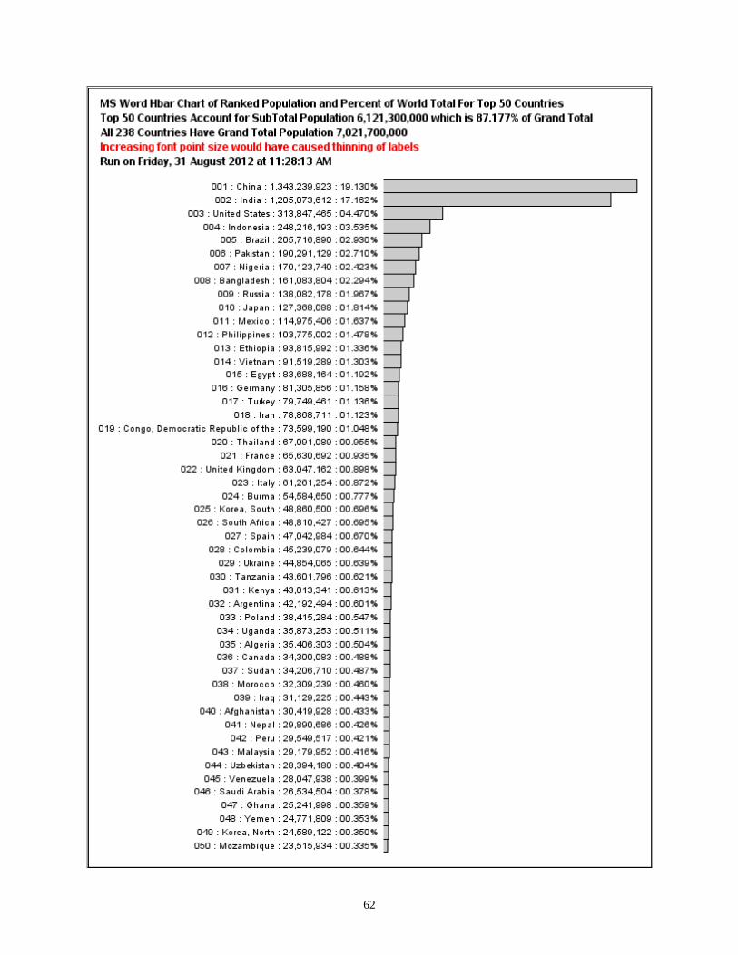
62

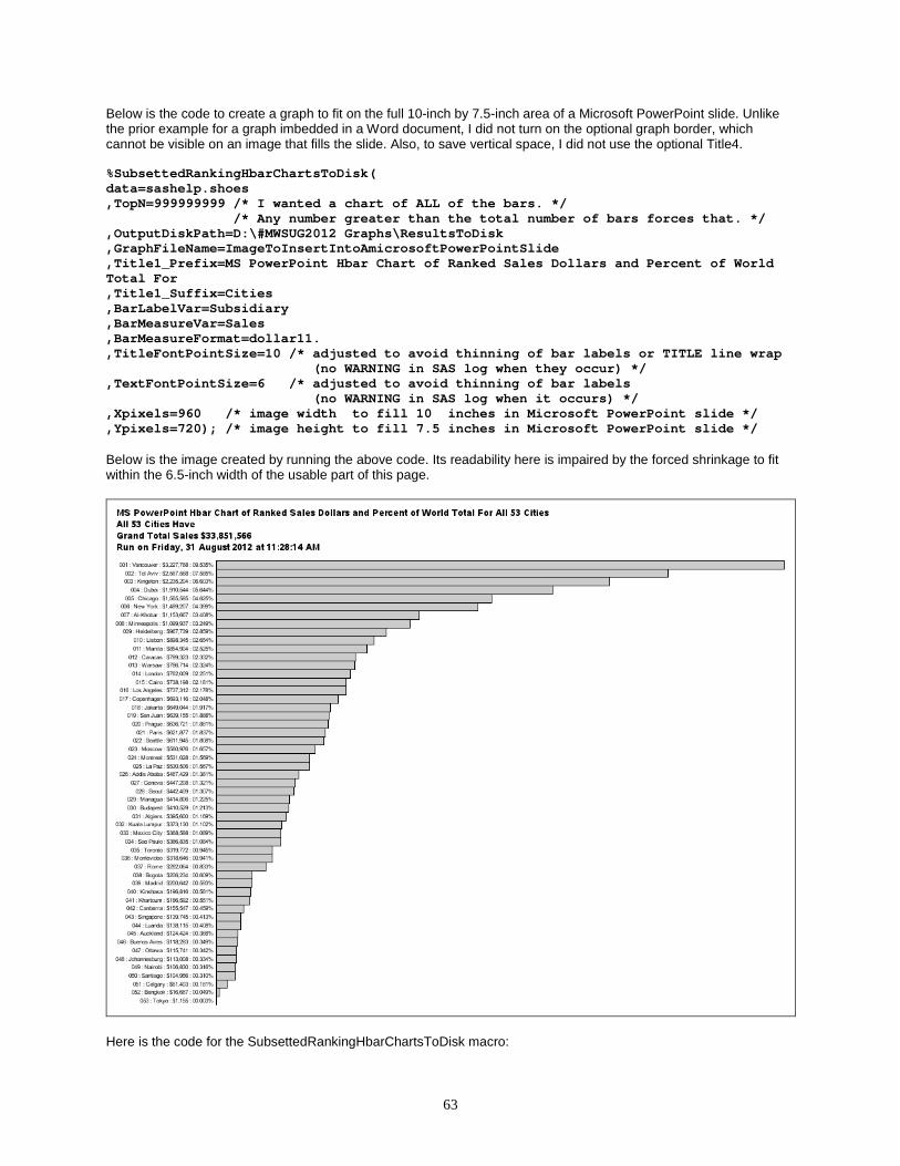
63

Below is the code to create a graph to fit on the full 10-inch by 7.5-inch area of a Microsoft PowerPoint slide. Unlike the prior example for a graph imbedded in a Word document, I did not turn on the optional graph border, which cannot be visible on an image that fills the slide. Also, to save vertical space, I did not use the optional Title4. %SubsettedRankingHbarChartsToDisk( data=sashelp.shoes ,TopN=999999999 /* I wanted a chart of ALL of the bars. */ /* Any number greater than the total number of bars forces that. */ ,OutputDiskPath=D:\#MWSUG2012 Graphs\ResultsToDisk ,GraphFileName=ImageToInsertIntoAmicrosoftPowerPointSlide ,Title1_Prefix=MS PowerPoint Hbar Chart of Ranked Sales Dollars and Percent of World Total For ,Title1_Suffix=Cities ,BarLabelVar=Subsidiary ,BarMeasureVar=Sales ,BarMeasureFormat=dollar11. ,TitleFontPointSize=10 /* adjusted to avoid thinning of bar labels or TITLE line wrap (no WARNING in SAS log when they occur) */ ,TextFontPointSize=6 /* adjusted to avoid thinning of bar labels (no WARNING in SAS log when it occurs) */ ,Xpixels=960 /* image width to fill 10 inches in Microsoft PowerPoint slide */ ,Ypixels=720); /* image height to fill 7.5 inches in Microsoft PowerPoint slide */ Below is the image created by running the above code. Its readability here is impaired by the forced shrinkage to fit within the 6.5-inch width of the usable part of this page.

Here is the code for the SubsettedRankingHbarChartsToDisk macro:

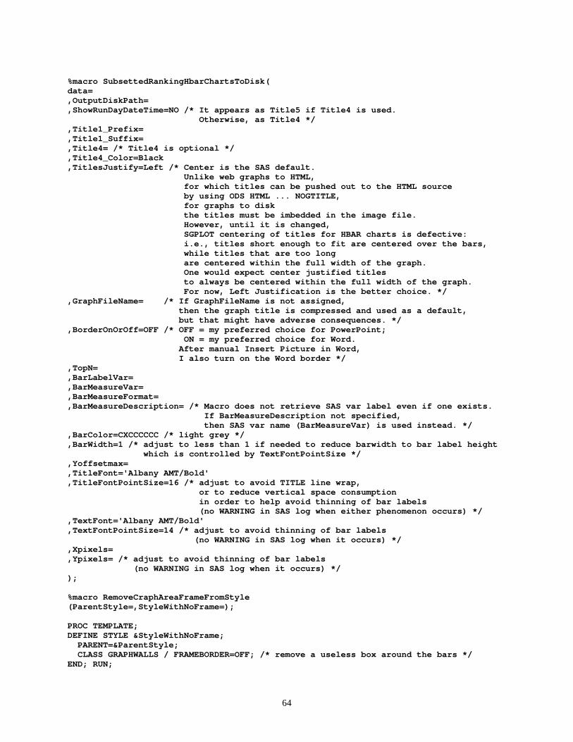
64

%macro SubsettedRankingHbarChartsToDisk( data= ,OutputDiskPath= ,ShowRunDayDateTime=NO /* It appears as Title5 if Title4 is used. Otherwise, as Title4 */ ,Title1_Prefix= ,Title1_Suffix= ,Title4= /* Title4 is optional */ ,Title4_Color=Black ,TitlesJustify=Left /* Center is the SAS default. Unlike web graphs to HTML, for which titles can be pushed out to the HTML source by using ODS HTML ... NOGTITLE, for graphs to disk the titles must be imbedded in the image file. However, until it is changed, SGPLOT centering of titles for HBAR charts is defective: i.e., titles short enough to fit are centered over the bars, while titles that are too long are centered within the full width of the graph. One would expect center justified titles to always be centered within the full width of the graph. For now, Left Justification is the better choice. */ ,GraphFileName= /* If GraphFileName is not assigned, then the graph title is compressed and used as a default, but that might have adverse consequences. */ ,BorderOnOrOff=OFF /* OFF = my preferred choice for PowerPoint; ON = my preferred choice for Word. After manual Insert Picture in Word, I also turn on the Word border */ ,TopN= ,BarLabelVar= ,BarMeasureVar= ,BarMeasureFormat= ,BarMeasureDescription= /* Macro does not retrieve SAS var label even if one exists. If BarMeasureDescription not specified, then SAS var name (BarMeasureVar) is used instead. */ ,BarColor=CXCCCCCC /* light grey */ ,BarWidth=1 /* adjust to less than 1 if needed to reduce barwidth to bar label height which is controlled by TextFontPointSize */ ,Yoffsetmax= ,TitleFont='Albany AMT/Bold' ,TitleFontPointSize=16 /* adjust to avoid TITLE line wrap, or to reduce vertical space consumption in order to help avoid thinning of bar labels (no WARNING in SAS log when either phenomenon occurs) */ ,TextFont='Albany AMT/Bold' ,TextFontPointSize=14 /* adjust to avoid thinning of bar labels (no WARNING in SAS log when it occurs) */ ,Xpixels= ,Ypixels= /* adjust to avoid thinning of bar labels (no WARNING in SAS log when it occurs) */ ); %macro RemoveCraphAreaFrameFromStyle (ParentStyle=,StyleWithNoFrame=); PROC TEMPLATE; DEFINE STYLE &StyleWithNoFrame; PARENT=&ParentStyle; CLASS GRAPHWALLS / FRAMEBORDER=OFF; /* remove a useless box around the bars */ END; RUN;

65

%mend RemoveCraphAreaFrameFromStyle; %RemoveCraphAreaFrameFromStyle (ParentStyle=Styles.Minimal ,StyleWithNoFrame=Styles.MinimalWithNoFrame); %if %length(&BarMeasureDescription) EQ 0 %then %let BarMeasureDescription = &BarMeasureVar; DATA _NULL_; RunDayDateTimeText = 'Run on ' || TRIM(LEFT(PUT(DATE(),weekdatx37.))) || ' at ' || TRIM(LEFT(PUT(TIME(),timeampm11.))); CALL SYMPUT('RunDayDateTime',TRIM(LEFT(RunDayDateTimeText))); RUN; PROC SUMMARY DATA=&data nway; CLASS &BarLabelVar; VAR &BarMeasureVar; OUTPUT OUT=Summed(drop=_type_ _freq_) SUM=; RUN; PROC SQL NOPRINT; SELECT COUNT(&BarLabelVar) , SUM(&BarMeasureVar) INTO :CountOfAllBars , :BarMeasureGrandTotal FROM Summed; QUIT; PROC SORT DATA=Summed; BY DESCENDING &BarMeasureVar; RUN; DATA All_WithBarLabels(drop=BarLabelSuffix); LENGTH BarLabel $ 256 BarLabelSuffix $ 7; SET Summed; BarLabelSuffix = TRIM(LEFT(PUT(((&BarMeasureVar / &BarMeasureGrandTotal) * 100),6.3))) || '%'; IF LENGTH(BarLabelSuffix) EQ 6 THEN BarLabelSuffix = '0' || BarLabelSuffix; BarLabel = TRIM(LEFT(PUT(_N_,z3.))) /* a bar count more than three digits will not fit on a PowerPoint slide or Word page */ || ' : ' || TRIM(LEFT(&BarLabelVar)) || ' : ' || TRIM(LEFT(PUT(&BarMeasureVar,&BarMeasureFormat))) || ' : ' || BarLabelSuffix; RUN; OPTIONS OBS=&TopN; DATA Selected_WithBarLabels; SET All_WithBarLabels; RUN; OPTIONS OBS=MAX; DATA ToChart; SET Selected_WithBarLabels; RUN; PROC SQL NOPRINT; SELECT COUNT(&BarLabelVar) , SUM(&BarMeasureVar) INTO :CountOfSelectedBars , :BarMeasureSubTotal FROM ToChart;

66

QUIT; DATA _NULL_; LENGTH ForSYMPUT ForSYMPUT1 ForSYMPUT2 8; ForSYMPUT = &BarMeasureGrandTotal; CALL SYMPUT('GrandTotal' ,TRIM(LEFT(PUT(ForSYMPUT,&BarMeasureFormat)))); ForSYMPUT = &BarMeasureSubTotal; CALL SYMPUT('SubTotal' ,TRIM(LEFT(PUT(ForSYMPUT,&BarMeasureFormat)))); ForSYMPUT = &CountOfAllBars; CALL SYMPUT('CountOfAll' ,TRIM(LEFT(PUT(ForSYMPUT,comma32.)))); ForSYMPUT = &CountOfSelectedBars; CALL SYMPUT('CountOfSelected',TRIM(LEFT(PUT(ForSYMPUT,3.)))); /* Word page or PowerPoint slide will never fit more than a 3-digit bar count */ ForSYMPUT1 = &BarMeasureSubTotal; ForSYMPUT2 = &BarMeasureGrandTotal; CALL SYMPUT('SubTotalPercentOfGrandTotal', TRIM(LEFT(PUT(( ForSYMPUT1 / ForSYMPUT2 ) * 100 , 6.3)))); RUN; %if %eval(&TopN GE &CountOfAllBars) %then %do; %let Title1 = &Title1_Prefix.%str( All )&CountOfSelected &Title1_Suffix; %let Title2 = All &CountOfSelected &Title1_Suffix Have; %let Title3 = Grand Total &BarMeasureDescription &GrandTotal; %end; %else %do; %let Title1 = &Title1_Prefix.%str( Top )&CountOfSelected &Title1_Suffix; %let Title2 = Top &CountOfSelected &Title1_Suffix Account for SubTotal &BarMeasureDescription &SubTotal which is &SubTotalPercentOfGrandTotal% of Grand Total; %let Title2 = %sysfunc(compbl(%nrquote(&Title2))); %let Title3 = All &CountOfAll &Title1_Suffix Have Grand Total &BarMeasureDescription &GrandTotal; %end; %if %length(&GraphFileName) EQ 0 %then %let GraphFileName = %sysfunc(COMPRESS(&Title1,' ')); ODS GRAPHICS ON / RESET=ALL BORDER=&BorderOnOrOff SCALE=OFF HEIGHT=&Ypixels.px WIDTH=&Xpixels.px IMAGENAME="&GraphFileName"; FOOTNOTE; ODS NORESULTS; ODS LISTING GPATH="&OutputDiskPath" STYLE=Styles.MinimalWithNoFrame; TITLE1 JUSTIFY=&TitlesJustify FONT=&TitleFont HEIGHT=&TitleFontPointSize PT "&Title1"; TITLE2 JUSTIFY=&TitlesJustify FONT=&TitleFont HEIGHT=&TitleFontPointSize PT "&Title2"; TITLE3 JUSTIFY=&TitlesJustify FONT=&TitleFont HEIGHT=&TitleFontPointSize PT "&Title3"; %if %length(&Title4) NE 0 %then %do; TITLE4 JUSTIFY=&TitlesJustify FONT=&TitleFont HEIGHT=&TitleFontPointSize PT COLOR=&Title4_Color "&Title4"; %end; %if %upcase(&ShowRunDayDateTime) NE 0 %then %do; %if %length(&Title4) EQ 0 %then %do; TITLE4 %end; %else %do; TITLE5 %end;

67

JUSTIFY=&TitlesJustify FONT=&TitleFont HEIGHT=&TitleFontPointSize PT "&RunDayDateTime"; %end; PROC SGPLOT DATA=ToChart; HBAR BarLabel / RESPONSE=&BarMeasureVar CATEGORYORDER=RESPDESC BARWIDTH=&BarWidth FILL FILLATTRS=(COLOR=&BarColor) OUTLINE; YAXIS DISPLAY=(NOLABEL NOLINE NOTICKS) VALUEATTRS=(SIZE=&TextFontPointSize) %if %length(&Yoffsetmax) NE 0 %then %do; OFFSETMAX=&Yoffsetmax %end; ; XAXIS DISPLAY=NONE; RUN; ODS LISTING Style=Styles.Listing; %mend SubsettedRankingHbarChartsToDisk;

68

CONCLUSION There are many, many useful features in SAS/GRAPH, which has been progressively improved over 33 years, and some of those features are regrettably missing in the new technology of ODS Graphics and SG procedures. The first macro provided here simplifies the task of overcoming a current limitation of the new technology. The third and fourth macros, to create subsetted ranked horizontal bar charts, implement a powerful and useful, though simple, concept and graphic method, and these macros work better when built with the new technology. REFERENCES 1. Holland, Philip R. “Anscombe's Quartet”, VIEWS News, Issue 54. UK: VIEWS International SAS Programmer

Community. 2011. http://www.sascommunity.org/wiki/VIEWS_News_backissues 2. Bessler, LeRoy. “The Most Communication-Effective and Most Usable Information Delivery”, Proceedings of the

SAS Global Forum 2010 Conference. Cary, NC: SAS Institute Inc. 2010. http://support.sas.com/resources/papers/proceedings10/231-2010.pdf

3. Bessler, LeRoy. “Communication-Effective Use of Color for Web Pages, Graphs, Tables, Maps, Text, and Print”, Proceedings of the Twenty-Ninth Annual SAS Users Group International Conference, Cary, NC, USA: SAS Institute Inc., 2004. http://www2.sas.com/proceedings/sugi29/176-29.pdf

4. Bessler, LeRoy. “Communication-Effective Pie Charts”, Proceedings of the SAS Global Forum 2007 Conference. Cary, NC: SAS Institute Inc. 2007. http://www2.sas.com/proceedings/forum2007/134-2007.pdf

5. Bessler, LeRoy. “All the Ways to Display Multiple Trend Charts”, VIEWS News, Issue 52. UK: VIEWS International SAS Programmer Community. 2011. http://www.sascommunity.org/wiki/VIEWS_News

6. Bessler, LeRoy and Riley, Alexandra. “All the Ways to Display Multiple Trend Charts: Three Selected Examples and Their Code”, VIEWS News, Issue 53. UK: VIEWS International SAS Programmer Community. 2011. http://www.sascommunity.org/wiki/VIEWS_News_backissues

7. Bessler, LeRoy. “Comparison of SAS Graphic Alternatives, Old and New”, Proceedings of the SAS Global Forum 2012 Conference. Cary, NC: SAS Institute Inc. 2012. http://support.sas.com/resources/papers/proceedings12/235-2012.pdf

8. Bessler, LeRoy. “%TRENDANO Macro for Collision-Free Automatic Annotation of Trend Plots”, Wisconsin Illinois SAS Users Conference Proceedings. Mequon, WI: Software User Services. 2001. For the latest report on this work, see http://www2.sas.com/proceedings/sugi27/p093-27.pdf for which Dr. Francesca Pierri was co-author.

9. Holland, Philip R. “Why Should You Be Using the New SG (Statistical Graphics) Procedures in SAS 9.2?”, Proceedings of the SAS Global Forum 2011 Conference. Cary, NC: SAS Institute Inc. 2011. http://support.sas.com/resources/papers/proceedings11/427-2011.pdf

AUTHOR INFORMATION Your comments and questions are valued and encouraged. Contact the author at:

LeRoy Bessler PhD Bessler Consulting and Research Converting Complexity Into Clarity™ Strong Smart Systems™ 262-242-1099 [email protected]

Dr. LeRoy Bessler has presented at software user conferences in the US, Canada, and Europe, on topics such as effective visual communication (using graphs, tables, web pages, or color), highly formatted Excel reporting from SAS, custom-developed tools to assist SAS server administrators, users, and managers, and Software-Intelligent Application Development methods to maximize Reliability, Reusability, Maintainability, Extendability, and Flexibility. His SAS experience includes application development and supporting users, servers, software, and data. SAS, SAS/GRAPH, and all other SAS Institute Inc. product or service names are registered trademarks or trademarks of SAS Institute Inc. in the USA and other countries. ® indicates USA registration. Other brand and product names are trademarks of their respective companies. Converting Complexity Into Clarity and Strong Smart Systems are trademarks of LeRoy Bessler PhD.

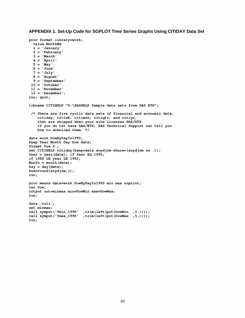
69

APPENDIX 1. Set-Up Code for SGPLOT Time Series Graphs Using CITIDAY Data Set proc format library=work; value MonthNm 1 = 'January' 2 = 'February' 3 = 'March' 4 = 'April' 5 = 'May' 6 = 'June' 7 = 'July' 8 = 'August' 9 = 'September' 10 = 'October' 11 = 'November' 12 = 'December'; run; quit; libname CITIHELP "D:\SASHELP Sample data sets from SAS ETS"; /* There are five cyclic data sets of financial and economic data, citiday, citiwk, citimon, citiqtr, and citiyr, that are shipped when your site licenses SAS/ETS. If you do not have SAS/ETS, SAS Technical Support can tell you how to download them. */ data work.DowByDayIn1990; keep Year Month Day Dow date; format Dow 5.; set CITIHELP.citiday(keep=date snydjcm where=(snydjcm ne .)); Year = year(date); if Year EQ 1990; if 1988 LE year LE 1991; Month = month(date); Day = day(date); Dow=round(snydjcm,1); run; proc means data=work.DowByDayIn1990 min max noprint; var Dow; output out=minmax min=DowMin max=DowMax; run; data _null_; set minmax; call symput('Ymin_1990' ,trim(left(put(DowMin ,5.)))); call symput('Ymax_1990' ,trim(left(put(DowMax ,5.)))); run;

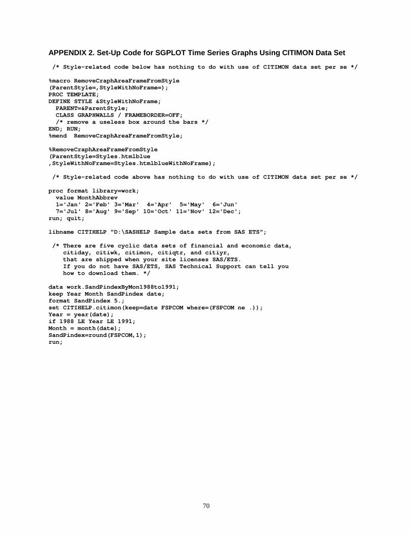
70

APPENDIX 2. Set-Up Code for SGPLOT Time Series Graphs Using CITIMON Data Set /* Style-related code below has nothing to do with use of CITIMON data set per se */ %macro RemoveCraphAreaFrameFromStyle (ParentStyle=,StyleWithNoFrame=); PROC TEMPLATE; DEFINE STYLE &StyleWithNoFrame; PARENT=&ParentStyle; CLASS GRAPHWALLS / FRAMEBORDER=OFF; /* remove a useless box around the bars */ END; RUN; %mend RemoveCraphAreaFrameFromStyle; %RemoveCraphAreaFrameFromStyle (ParentStyle=Styles.htmlblue ,StyleWithNoFrame=Styles.htmlblueWithNoFrame); /* Style-related code above has nothing to do with use of CITIMON data set per se */ proc format library=work; value MonthAbbrev 1='Jan' 2='Feb' 3='Mar' 4='Apr' 5='May' 6='Jun' 7='Jul' 8='Aug' 9='Sep' 10='Oct' 11='Nov' 12='Dec'; run; quit; libname CITIHELP "D:\SASHELP Sample data sets from SAS ETS"; /* There are five cyclic data sets of financial and economic data, citiday, citiwk, citimon, citiqtr, and citiyr, that are shipped when your site licenses SAS/ETS. If you do not have SAS/ETS, SAS Technical Support can tell you how to download them. */ data work.SandPindexByMon1988to1991; keep Year Month SandPindex date; format SandPindex 5.; set CITIHELP.citimon(keep=date FSPCOM where=(FSPCOM ne .)); Year = year(date); if 1988 LE Year LE 1991; Month = month(date); SandPindex=round(FSPCOM,1); run;