Geotechnical Synergy in Buenos Aires 2015 A.O. Sfriso et ... · additives, and is removed from the chamber mechanically, through a screw conveyor. In slurry pressure balance (SPB)

TBM Pressure Models – Observations, Theory and Practice

Tiago Gerheim Souza DIASa,1 and Adam BEZUIJENa,b a

Ghent University, Ghent, Belgium b

Deltares, Delft, The Netherlands

Abstract. Mechanized tunnelling in soft ground has evolved significantly over the last 20 years. However, the interaction between the tunnel boring machine (TBM) and the ground is often understood through idealized concepts, focused mostly on the machine actions in detriment of the reactions from the ground. These concepts cannot be used to explain several mechanisms that have been observed during the construction of mechanized tunnels. Therefore, this paper presents the path from field observations to the theoretical developments to model the TBM-ground interaction more realistically. Some ideas on how these developments can be applied into practice are presented. Finally, a discussion is proposed about how an effective collaboration between academia and industry can alleviate the current concentration of knowledge in the state of practice.

Keywords. Mechanized Tunneling, Grout Pressure, Face Pressure, Rheological Models

1. Introduction

This paper is the extended written version of a presentation delivered by the first author at the panel session "Excavations and Tunnels" of the XV Pan-American Conference on Soil Mechanics and Geotechnical Engineering. The structure of the paper adheres to the oral presentation, where three questions were answered by each panelist. The first question (Section 2) was set individually, while the second (Section 3) and third (Section 4) questions were set for all panelists alike. The presentations were followed by a general discussion with the panel members and the audience.

The main subject of this paper is mechanized tunnel construction in soft ground, which has evolved significantly over the last 20 years especially on the issue of settlement control. This is normally traced back to a more precise operation of the tunnel boring machine (TBM), with special consideration to the control of the face pressure and the injection of the soil-lining void trough the tail of the TBM. As a consequence, mechanized tunnels are being considered viable options for projects with strict limits of disturbance, where underground solutions were deemed unsuitable in the past.

Figure 1 presents the main elements of a soft ground TBM. The internal structure is particular of an earth pressure balance machine (EPB), but the geometric details highlighted on the bottom of the figure are similar for all TBMs. The cutting tools, positioned at the cutterhead (A), loosen the soil at the tunnel face.

1 Corresponding Author.

Geotechnical Synergy in Buenos Aires 2015A.O. Sfriso et al. (Eds.)IOS Press, 2015© 2015 The authors and IOS Press. All rights reserved.doi:10.3233/978-1-61499-599-9-347

347

Figure 1. Basic structure of a TBM with highlight to the progressive diameter reduction from the cutterhead (A), to the front (B) and back (C) of the shield and the lining extrados (D).

As the soil flows through the openings at the cutterhead, into the excavation

chamber (B), it blends in the supporting mixture, which is kept pressurized to support the face. The system that controls how the spoils are extracted from the chamber is also responsible for keeping the pressure stabilized between the tunnel face and the bulkhead. In EPB machines, the mixture is composed of the excavated soil and additives, and is removed from the chamber mechanically, through a screw conveyor. In slurry pressure balance (SPB) and mixshield machines, the mixture is mostly composed of a slurry suspension, and is removed through a hydraulic circuit. The chambers of mixshield machines are divided by a submerged wall, in a working chamber, completely filled with slurry, and a pressure chamber, partially filled with a pressurized air bubble that controls the pressure at the chamber.

The diameter of the cutterhead determines the size of the excavated boundary (A), which tends to be larger than the front of the TBM shield (B). The shield is always tapered, so the front diameter (B) is slightly larger than the diameter at the back (C). After the lining segments are combined in a ring inside the shield, the machine thrusts itself forward, leaving the lining in contact with the ground (D). From the moment the cutterhead passes a cross-section, the structure from the TBM to the tunnel lining presents a progressively smaller diameter to support the excavation. To mitigate the convergence of the soil from A to D (see Figure 1), grout is injected from the back of the shield. To prevent water or grout from coming in the TBM, the contact between the shield and the lining is sealed with steel brushes filled with pressurized grease [1].

These basic principles are essential to discuss how the interaction mechanisms between the soil and the TBM are often interpreted within idealized frameworks that do not account for some observed features of the soil response. In response to that, the path from field measurements to theoretical developments is traced in Section 2. Some ideas on how these developments can be applied into practice and even incorporated in the usual methods to estimate the tunneling induced displacements and the lining forces are presented in Section 3. Finally, it is argued that an unbalanced concentration of

T.G.S. Dias and A. Bezuijen / TBM Pressure Models – Observations, Theory and Practice348

knowledge in the industry can jeopardize engineering practice. Some ideas on how these effects can be alleviated, through an effective collaboration between academia and industry, are discussed in Section 4.

2. What do you understand is missing in evaluating soft ground response to tunnelling with modern TBM technologies?

To answer that, one should consider that an innate feature of mechanized tunnelling is that every step of the excavation cycle is performed through mechanical or hydraulic systems that compose the tunnel boring machine (TBM). The interaction mechanisms between the TBM and the surrounding ground result from the operation of these systems to excavate and support the ground around the tunnel. It is self-evident that for each of these actions there will be a reaction from the ground to achieve equilibrium. However, these mechanisms are often interpreted within idealized frameworks that do not account for important features of the ground reaction that have been observed in the field. Therefore, these frameworks need to be adapted to account for the interaction between the TBM and the ground.

These should consider how the geotechnical aspects of the ground reaction and the rheological properties of the excavation fluids (foam, bentonite, and grout) affect the mechanisms around the TBM. This section presents a scheme for the TBM-ground interaction divided in four elements: face pressure, flow around the TBM, tail void grouting and lining equilibrium [2]. Each element is contrasted between the ideal mechanism and the observed ground responses. And, wherever possible, an alternative framework is presented.

2.1. Face pressure

The face of a TBM is the most erratic zone to define conceptual boundaries for a theoretical model. The cutterhead rotates and the cutting tools scrape the ground from the tunnel face while additives are injected to condition the material. Water, polymers, bentonite and foam can be used under different conditions [3]. The loosened ground with additives, herein referred to as mixture, flows through the openings at the cutterhead and in the excavation chamber until it reaches the screw conveyor or the hydraulic circuit. The structure of the mixture is very important to understand how the face pressure is transferred to the tunnel face. The slurry suspensions on SPB and mixshield machines, which can be extracted through a hydraulic circuit, are normally more fluid than the paste consistency necessary to control the pressure gradient along the screw conveyor on EPB machines. However, in both cases, the mixture presents a very open matrix, where the solid particles are in a suspension with negligible effective stresses. The rheology can then be considered equivalent to a fluid and, as the mixture flows slowly, viscous forces are not considered at this point.

These fluid mixtures can only support isotropic stress states, represented by an equivalent scalar pressure. Adversely, the undisturbed ground at the tunnel face will, in most cases; be standing under an anisotropic stress state, set by the coefficient of earth pressure at rest (k0). Therefore, it is fundamentally unfeasible to transfer a face pressure that will match the in-situ stress of the ground in every direction, due to the basic fact that the supporting mixture cannot stand it (Figure 2).

T.G.S. Dias and A. Bezuijen / TBM Pressure Models – Observations, Theory and Practice 349

Figure 2. Differences between the stress states of the supporting mixture (fluid) and the ground (solid).

As a consequence, the tunnel face will always undergo stress increments, and the

associated strains. Along the radial direction, the excavated perimeter can either contract or expand. If it contracts while in contact with the cutterhead, an additional volume of ground will be excavated. For an expanded section, there will be a gap between the ground and the cutterhead. This allows the supporting mixture to flow around the shield depending on the hydraulic gradients. Another point to consider is that if volumetric strains are induced in a saturated ground, they will generate increments of pore water pressure that will lead to consolidation. Of course, the time frame for dissipation will depend on the ground permeability and drainage conditions.

The fact that the supporting mixture has such a loose matrix that it acts as a fluid raises the question of whether the face pressure should be considered by its hydraulic head or just as a total stress boundary. Here, a parallel is normally traced with slurry walls, where the supporting fluid creates an impermeable layer on which the fluid pressure is applied and the hydraulic head is dissipated. In this way, the pressure can be transferred to the ground without changing the hydraulic boundary conditions. The same thing should occur at the TBM face, through the so-called filter cake. However, one should consider that the ground at the tunnel face is constantly being removed while the filter cake is being formed, which can affect the process.

This problem was identified when excess pore pressures were measured in front of SPB [4,5] and EPB machines [6], revealing that the ideal process of cake formation is not always achieved and depends on the properties of the ground, the additives and the excavation speed (see Figure 3). To quantify these effects, one must first understand how the supporting fluid creates an impermeable layer on the ground. The pressure in the supporting fluid must be higher than the water pressure in the ground, inducing the fluid to flow into the ground. The fluid carries suspended material that clogs the ground pores, reducing its permeability. As far as this process is concerned, the foam bubbles to condition permeable soils on EPB TBMs have the same purpose as the slurry particles on SPB and mixshield TBMs.


Figure 3. Measurements of excess pore water pressure in front of SPB and EPB tunnels

The second step is to quantify the gradient inducing the flow from the face. An

analytical formulation can be derived [4], based on the approximation that there is an infinitesimal constant hydraulic source all over the tunnel face. This distributed head is defined with reference to the in-situ water pressure. By equating the volumetric flow rate from the source (A=dr.r.dθ) with the one at a certain radial distance (s) along a semi-spherical domain in front of the tunnel (A=2.π.s²), one obtains:

2..4.....

2sdsdkdrdrq �� (1)

where q is the discharge from the point source, assumed constant all over the tunnel face.

By integrating Eq. 1 along the following limits: ϕ=[ϕ(S),∞]; s=[S,∞]; r=[0,R]; θ=[0,2π], and defining 22 rxs � , one obtains:

� � � �xRxR

x � 220�� (2)

where ϕ0 is the incremental piezometric head at the tunnel face (x=0). From Eq. 2 it is possible to calculate the hydraulic gradient at the tunnel face as:

RRxx

Rdxd

xx

0

022

0

0

1 ��

�

��

�

�

(3)

The penetration velocity can then be defined as:

0

10

20

30

40

50

60

70

80

90

0 10 20 30 40

exce

ss p

ore

pres

sure

-φ

(kPa

)

distance from tunnel face - x (m)

SPBSPT - FitEPBEPB - Fit

SPB EPB φ0 55 120 R 4.25 4.325

� �xRxR

� 220��


Rnkvp .. 0� (4)

where n is the ground porosity and k is the ground hydraulic conductivity to the penetration fluid.

Therefore, the face pressure should be kept at a certain pressure so that the supporting fluid can penetrate the ground faster than the excavation velocity. Otherwise, the excavation tools will always be scraping deeper than the fluid penetration, cancelling the effect of an impermeable layer. In this case, the hydraulic head of the supporting fluid is not dissipated and groundwater flow from the tunnel face to the ground is induced. There are some recent attempts to model this process numerically with a surrogate model for the slurry penetration [7].

The increments of pore water pressure in front of the tunnel can affect the face stability and the tunnel interaction with surrounding structures. On top of that, the water outflow has special consequences for foam conditioning, which depends heavily on the amount of water on the supporting mixture. The foam is formed by mixing a surfactant solution, which presents a certain liquid volume (QL), with compressed air. This forms a structure where pockets of gas are trapped in the foam bubbles. The volume of foam (QF) is used to calculate the foam expansion ratio (FER=QF/QL), diving it by the original liquid volume of the solution, and the foam injection ratio (FIR=QF/QS), dividing it by the volume of excavated ground (QS). Once the foam blends in the supporting mixture, its additional volume will increase the initial porosity of the mixture (n1), described in Figure 4a, to a porosity that is suitable for the TBM operation (n2). For an initially dry mixture, the foam will occupy the air spaces (Figure 4b), so the necessary volume of foam to increase the porosity from n1 to n2 can be calculated as:

� �2

12)(

11

nnnVV i

dryF

� (5)

If the mixture is originally saturated, one must consider the possibility that the face pressure will induce groundwater flow from the face, in which case the initial amount of water will be reduced or even increased, depending on the flow conditions. Considering the hypothesis that there is no water flow (Figure 4c), the necessary volume of foam can be calculated as:

2

12)(

1 nnnVV i

flownoF

� (6)

For the case where water flows out of the mixture (Figure 4d), the necessary volume of foam can be calculated as:

� ��

��

��

�

� FWRnnnnVV

nnnVV iWi

flowF .

111

12

122

2

12)( (7)

where the Foam Water Replacement Ratio (FWR) is defined as the volume of water that flow out of mixture over the initial volume of water.


Figure 4. Representative volumetric elements for the solid, water and foam fazes in a supporting mixture

Using Eqs. (5), (6) and (7) one can calculate the necessary FIR for these three

conditions. A detailed calculation example is presented on Section 3.1.

2.2. Flow around the TBM

While a certain cross-section is between the face and the tail, the general understanding is that structure of the TBM shield is what supports the excavation. Then, when the shield is propped forward, it leaves a fully assembled lining ring as permanent support. It was already discussed how the diameter of the shield is progressively smaller from the cutter head to the tail of the TBM (Figure 1). It is reasonable to consider, for current machines, that the cutterhead excavates a diameter 1 to 3 cm larger than the front of the shield (over-excavation) and that along the shield the diameter reduces about 0.4 % [8,9]. The volume loss due to the convergence of the excavation boundary can then be calculated as:

2

11 ��

��

� �

excL R

RV (8)

where ΔR is the radial convergence and Rexc is the excavation radius. Considering a tunnel of 10 m in diameter and an over-excavation of 3 cm, the

radial convergence comes to 3.5 cm, which is equivalent to a volume loss of 1.4 %. This volume loss around the tunnel can be assumed equal to the volume of the settlement trough, provided that the excavation does not induce volumetric strains [10]. In this case, if the mechanism is correct, the minimum volume loss due to a TBM excavation would be the one imposed by its geometric characteristics. However, it is not uncommon nowadays to achieve volume losses as low as 0.2 %. This observation led to the proposition of a different mechanism for the ground interaction around the shield.

For this process, both the grout, injected at the back of the TBM, and the mixture, supporting the tunnel face (Section 2.1), are considered to act as fluids. As such, provided there is a longitudinal pressure gradient and gap between the soil and the shield, these fluids will flow around the TBM. The resultant pressure distribution controls the tunnel convergence and prevents the complete closure of the soil-shield


gap. To simulate this process it is necessary to model the viscous flow of the excavation fluids and the relation between the boundary pressures and the excavation convergence.

The mechanical response of the grout and the supporting mixture can be modeled as Bingham plastic fluids. In this model, the material behaves as a rigid body until a limit shear stress is reached, from where it starts to flow as a viscous fluid. In this formulation the shear stress can be described as:

dydu

y �� (9)

where τy is the yield resistance, η is the dynamic viscosity and du/dy is the velocity gradient perpendicularly to the flow.

There are several techniques available to characterize these parameters [11]. If small velocities are considered, the second term of Eq. (9) can be disregarded and the shear stress assumed equal to the yield resistance. This is a reasonable assumption for the flow around the TBM and it simplifies the calculation process. However, while it does not require the assumptions of the shear rate distribution in one hand, it turns the model unable to solve the velocity field in the other. In this way, considering the flow between the soil-shield gap to be equivalent to a flow between parallel plates, the pressure dissipation due to one interface can be calculated as:

gapl

p y ��.� (10)

where Δl is the distance along the flow direction, defined in the same unit as the gap. The gravitational field can be disregarded at this stage.

The other element of the simulation is the relation between the boundary pressures and the excavation convergence. In a homogeneous, isotropic and elastic medium, under isotropic stress conditions (k0=1), a linear relation can be traced between the tunnel convergence (∆r) and an axisymmetric stress release (∆σ) around the tunnel:

Grr�

� 2� (11)

where G is the shear modulus and r is the initial radius of the tunnel. Figure 5 presents the results of Eq. (11) for a tunnel with 5 m initial radius,

13 MPa shear modulus of the ground and 500 kPa initial in-situ stress. These two models can be programmed in a spreadsheet to simulate 1D flow around

the TBM and obtain the resultant pressures and convergences. An example result is presented in Figure 6 considering the following parameters: 5 m excavated radius; 400 kPa initial in-situ stress; 50 MPa ground shear modulus; 300 kPa face pressure; 600 kPa grout pressure; 5 m long shield; 1 cm over-excavation; 1 cm tapering; 1.5 kPa grout yield strength; 80 Pa mixture yield strength (equivalent to bentonite). The results indicate that the ground does not come in direct contact with the shield. As the face pressure is smaller than the in-situ stress, the excavation converges about 50 mm around the front of the shield. The bentonite then flows back 1.25 m along the soil-shield gap. On the other hand, the grout pressure is higher than the in-situ stress, which


causes the excavation to expand about 100 mm. The grout then flows back 3.75 m along the gap with a steep pressure drop. In this set-up, the volume loss just after the cutterhead is about 0.2 % while at the tail of the TBM is -0.4 %, which is in better agreement with measured values.

Figure 5. Relation between the boundary pressures and the excavation convergence for a tunnel with 5 m

initial radius, 13 MPa shear modulus and 500 kPa initial in-situ stress.

Figure 6. Example calculation for the flow around the TBM

0

100

200

300

400

500

600

700

800

900

1000

-10 -5 0 5 10

Boun

dary

Pre

ssur

e (k

Pa)

Stre

ss In

crea

seSt

ress

Rel

ease

Contraction Expansion

UndisturbedCondition

Grr�

� 2�

Δr (cm)

4.980

4.990

5.000

5.010

0

100

200

300

400

500

600

0 1 2 3 4 5

Radi

us (m

)

Boun

dary

Pre

ssur

e (k

Pa)

Distance from the tunnel face (m)

CavityShield

GroutPressure

FrontShield

BackShield

FacePressure

FaceMixture

Grout

ExcavatedRadius


2.3. Tail void grouting

The previous section already highlighted how the pressure of the grout that is injected at the TBM tail will determine the expansion/convergence of the excavated boundary and the flow pattern around the TBM shield. However, the main purpose of the grout injection is to fill the gap between the back of the shield and the lining ring (Figure 1). The diameter of the lining is normally 1.5 to 8% smaller than the back of the TBM, which is equivalent to a tunnel volume loss between 3 and 15% for full gap closure [12].

The process of tail grouting is, at times, understood as a volumetric problem. The logic goes as follows: Once the TBM is trusted forward, it leaves behind a gap between the soil, which was previously supported by the shield, and the lining ring that was left in place. So, by injecting a volume of grout equal to the volume of the gap, soil convergence can be avoided. However, this logic fails whenever the ground deforms faster than the process described and/or the previously injected grout is still fluid. Both of these conditions can be assumed for most regular cases. Therefore, the focus has to change from controlling the injected volume to keeping the gap pressurized.

Field measurements were performed during the excavation of the Sophia Rail tunnel, a 4.2 km twin tunnel with an external diameter of 9.5 m and a 0.4 m thick concrete lining. The tunnel crown was located at a depth of 14.77 m where the overburden pressure was approximately 200 kPa. A single component grout was used in the tail void. In each tunnel, one full-ring of the lining was instrumented with 14 pressure sensors, monitored from the moment the rings were placed to about 11 hours after leaving the shield. A detailed analysis of the data can be found in [13]. For the sake of objectiveness, the time series of all instruments is combined in two averages: grout pressure and vertical gradient, where most relevant aspects can be seen (Figure 7).

Figure 7. Measurements of average grout pressures and vertical gradients with time


The time is set from the moment the lining comes in contact with the grout. When the TBM was excavating and advancing, grout was constantly being injected in the gap. This caused the pressures to increase during drilling, with some oscillations in the first two cycles due to the process of ring building. During stand still, on the other hand, the pressure decreased. Just before the first two cycles, one can see a considerable decrease in the grout pressure. This happened because the TBM advanced a few seconds before the grout pumps were activated, illustrating the fallacy of understanding the process of tail void grouting as a volumetric problem. For the fourth cycle onwards, the grout injections on the TBM tail were not noticed anymore while the pressure decrease still continued, though with a smaller magnitude. Focusing on the vertical gradients around the lining, there were also marked differences between the phases of drilling and stand-still. When the grout was injected, during the first cycles, the gradient was around 20 kPa which is equivalent to the grout volumetric weight. During stand-still there was a sharp decrease to about 15 kPa followed by a reduction with time to about 10 kPa.

Qualitatively, these results can be understood as follows: While the grout is being pumped, the flow direction is predominantly longitudinal so only the gravity field determines the vertical gradient. During stand-still, the grout flows along the tangential direction of the cross-section. As the grout pressure dissipates due to shear, the vertical gradient is reduced just after drilling stops. With time, as the grout pressures are higher than the local groundwater pressure, the grout loses water to the ground. This consolidation process progressively reduces the grout pressure, while the vertical gradient tends to reach the gradient of the groundwater. As the grout starts to harden and the consolidation advances, the pressure variations due to new injections are no longer noticeable.

To obtain quantitative results, each of these processes needs to be modeled. The pressure increase during the excavation is a direct consequence of the operation of the grout injection system. A pressure controlled operation can be calculate based on mechanical equilibrium. As, for the volume controlled case, the pressure field can only be determined considering a compressible fluid, where the energy and the mass conservation/momentum equations can be linked. It should be noted that, in these formulations, the operational feasibility of the system, such as achievable discharge, frequency of maintenance and necessary backup utilities, are not directly assessed, but should always be verified with the mechanical design team.

The first aspect to be considered for the phase of stand-still is the tangential grout flow. Overall, this problem can be formulated is a similar way to the TBM Flow, modeling the flow of a viscous plastic fluid in equilibrium with a deformable boundary [14]. The same rheological grout model (Bingham plastic fluid, with τ=τy) is assumed to calculate the pressure field around each injection nozzle, where the pressure boundary conditions of the problem are stated. Referring to Figure 8, the pressure at point B can be calculated from the injection pressure of the nozzle, at point A as:

dhdlgap

pp gg

AB .. ��

(12)

where dl is the distance along the flow path, dh is the vertical distance and γg is the volumetric weight of the grout.


Figure 8. Elements to model the tangential grout flow

The pressure at point C is then calculated similarly as:

dhdlgap

pp gg

AC .. ��

� (13)

The simplest approach to deal with multiple nozzles (6 to 8 in a regular TBM) is to calculate the pressure field around the whole domain for each individual nozzle and assume that the maximum pressure at each point around the perimeter composes the resultant field [15]. For a constant gap, these equations can be programmed in a spreadsheet to calculate the grout pressures in a discrete set of points along the tunnel perimeter. However, the ground deformation in equilibrium with the grout pressures should also be considered. Similarly to the TBM flow model, the gap between the tunnel and the lining can be assessed through a relation between the boundary pressures and the excavation convergence/expansion. The isotropic model from Eq. (11) can be used, observing its limitations. Together, these two models can be programmed in a spreadsheet to simulate the 2D flow around the lining and obtain the results of pressure and convergence.

An example result is presented in Figure 9 considering the following parameters: 5 m excavated radius; 15 cm initial tunnel-lining gap; 30 m tunnel center depth; 45 MPa ground Young’s modulus, 0.3 ground Poisson’s ratio; 20 kN/m³ ground volumetric weight; 0.5 coefficient of earth pressure at rest; groundwater level at the surface; 0.5 kPa grout yield strength; 20 kN/m³ grout volumetric weight. A layout of six injection nozzles was considered, each one with an injection pressure of 400 kPa. The results indicate a profile of grout pressures with an average vertical gradient of 14 kPa, which is similar to the in-situ normal stress at the tunnel springline. As the grout pressure is smaller than the normal stress at the tunnel roof and invert, the excavation converges, in an average of 1 cm, which is equivalent to a volume loss of 0.4%. The grout pressures can also be used to assess the resultant vertical force acting on the lining ring. For this set up an upwards force of 1170 kN/m was calculated. Further implications of this force will be discussed in the following section.


Figure 9. Example calculation for the tangential grout flow in terms of the soil-lining gap (left) and the

boundary pressures (right).

The second aspect to be accounted for is the consolidation of the grout, which is

responsible for the decrease of both the gradient and magnitude of grout pressures during stand-still [16]. The geotechnical aspect of this process, which is sometimes called grout filtration, is analogous to the one described for the face pressure transfer. But here there is no reason to assume that a filter cake is formed in the ground, so only an external layer of filtered grout is considered. Therefore, the water flow from the grout to the ground will depend on the difference in water pressure between both regions, the permeability of the filtered grout and its thickness. A scheme of the process can be seen in Figure 10 for 1D conditions. The slurry grout is characterized by its initial volume (V0) and porosity (ni). The filtered grout is characterized by its porosity (nf).

Figure 10. Volumetric scheme for the process of grout consolidation


Considering incompressible fluids and a constant volume of solids, the continuity equations is:

� �� dx

nnn

dtqi

fi

1. (14)

where q is the water discharge, which can be calculated through Darcy’s law. The loss of hydraulic head within the slurry is negligible, so the pressure in the

slurry can be considered constant. When the permeability of the ground and the filtered grout are of the same order of magnitude, the hydraulic head will dissipate through both layers, increasing the groundwater pressure nearby [17]. On the other hand, in fine sand or coarser grained soils it very likely that the permeability of the ground is significantly higher than the one of the filtered grout. In this case, the dissipation through the ground can be neglected, so that all the pressure difference between the groundwater and the grout is dissipated through the filtered grout layer [16]. The following derivations assume the second case. By substituting the discharge equation (q=k.Δϕ/x) in Eq. (14), assuming a constant difference in piezometric head (Δϕ), and integrating with x(0)=0 as a boundary condition, one obtains:

� � � �� tk

nnntx

fi

i ...21 ��

(15)

where x is the thickness of the filtered grout layer, k is the permeability of the filtered grout, Δϕ is the pressure difference between the groundwater and the grout, and t is the time.

The process will stop once all the slurry grout has been filtered or the driving force (the pressure difference) is no longer present. The time necessary to reach this stage can be calculated as:

� ��

202max .

..2.1.1

hkn

nnnt

f

fii

��

(16)

where h0 is the initial thickness of the slurry grout. However, normally the difference in piezometric head is not constant. The

pressures should be in equilibrium with the tunnel boundary, so the deformability of the ground needs to be considered. The isotropic model from Eq. (11) can be used, observing its limitations. Assume that the consolidation process starts from an equilibrium condition, so that the grout pressure is equal to the tunnel boundary pressure. From this stage, the volume reduction due to the consolidation of the grout will lead to the convergence of the boundary and the related reduction in pressure (see Figure 5). In other words, the grout pressure will reduce as the grout consolidates due to the stress release of the deformable ground. Assuming that all grout phases are fully saturated, the reduction of the initial grout volume is equal to the volume of water expelled from the slurry, which can be obtained through the direct integration of Eq. (14). If this variable is set as Δr from Eq. (11), and the resulting Δσ is discounted from the initial pressure difference Δϕ, one obtains a new form for the thickness of the filtered grout:


� �� dtkx

RG

nnndxx

fi

i ...21. ��

��

��

� (17)

The solution of this equation is by no means trivial. However, if the first computation of dx is done with a very small dt through Eq. (15), the calculation can proceed numerically, where each computation of dx is based on the previous computation of x. Even in the incremental form it is possible to obtain the maximum thickness of the filtered grout as:

� �� fi

i

dtdx

nnn

GRx

�

1.2

.0max

� (18)

An example calculation of these 1D models is presented in Figure 11 considering the following parameters: 0.4 porosity of the slurry; 0.3 porosity of the filtered grout; 500 kPa grout pressure; 400 kPa ground water pressure; 15 cm initial grout thickness; 10-8 m/s filtered grout permeability; 50 MPa ground shear modulus; 5 m initial tunnel radius. The results show a remarkable difference between the calculations with constant and variable boundary pressures. The first aspect is that the constant pressure can build up a much thicker layer of filtered grout, as the grout will be completely dewatered. On the other hand, the case with a deformable boundary rapidly decreases the pressure, reaching equilibrium with the groundwater and stopping the process while part of the grout is still in slurry form. The consolidation led to 0.5 cm of convergence, which corresponds to 0.2 % volume loss.

The main feature to be acknowledged is that the grout pressures will converge to the groundwater pressures. Even though this was not directly modeled, one can apply the concept for the whole tunnel perimeter, which will result in a decreasing pressure magnitude and vertical gradient equivalent to the gradient due to the water weight. Both conclusions are in direct agreement with the field observations (see Figure 7).

Figure 11. Example calculation of grout consolidation with constant a variable boundary pressure

300

350

400

450

500

0.0

3.0

6.0

9.0

12.0

0 5 10 15 20

Pres

sure

(kP

a)

Filte

red

Grou

t (c

m)

Time (min)

φ constant

φ variable


2.4. Lining equilibrium

The lining equilibrium is directly dependent on the pressure gradients of the grout, as they are in direct contact after the ring leaves the tail of the TBM. Through the aforementioned mechanisms, the lining can be seen as a buoyant structure immersed in a pressurized viscous fluid that is flowing as it hardens and consolidates [13]. The first aspect to be considered is that the vertical gradient of the grout pressures result in an upwards force acting on the lining, which might not be in balance with the weight of the lining. The calculation example from Figure 9 reached a resultant upward force of 1170 kN/m. Considering an external radius of 4.85 m, a typical lining ring thickness of 50 cm, and a volumetric weight of 25 kN/m³, the full lining ring weighs about 360 kN/m. The net result of these two forces is 800 kN/m upwards.

If the forces are unbalanced in an individual lining section, the lining is forced to move upwards until either the resultant grout pressures match the lining weight or the lining comes in contact with the roof of the ground cavity, which will then react until equilibrium is reached. One way to reduce the net force is to re-design the injection layout and/or the grout properties. Keeping all the other parameters constant, the same example results in a null net force for a grout with 1.8 kPa of yield strength instead of the original 0.5 kPa. However, as just discussed, the gradient of grout pressure is bound to change with time due to consolidation, so it is inexorable that in one stage or the other there will be a non-null net force acting on the lining.

Another way to look at this problem is to consider the rings to be interlocked in the longitudinal direction, so that all lining rings respond together. This process can be modeled through an equivalent 1D beam. One possibility is to represent the TBM jacking forces in one end and the hardened grout in the other. The time for the grout to harden will correspond to a certain number of installed rings that will set the length of the equivalent beam [13]. This approach has been successfully applied to reproduce measurements of vertical lining movements [18]. For fast settling grouts, where the length of the liquid phase is small when compared to the tunnel diameter, the 1D hypothesis will probably be unsuitable and more complex models are needed. Another possibility is to consider a semi-infinite beam set partially on the liquid grout and partially on an elastic foundation that represents the hardened grout (Figure 12). The analytical solution of this problem has been used to reproduce measurements of the lining bending moments and inclination [19].

If the resultant displacements are excessive, the relative movement between the rings can lead to steps in the tunnel and damage to the circumferential joints, movements along the radial joints and even structural damage to the lining.

Figure 12. Lining model scheme as a 1D equivalent beam on a semi-infinite elastic foundation.

TBM

liquidgrout

beam on elastic foundation

q1q2

k

MTBM

QTBM

qgrout


3. From your perspective and experience, what do you see as the currently mostly needed improvement in the design or construction practice of urban underground excavations?

From Section 2 one should be aware that to understand the TBM mechanisms, which have been traditionally presented as simple mechanical processes, it is essential to consider the geotechnical aspects of the TBM-ground interaction along the different excavation phases.

The observed consequences of this interaction have been presented together with theoretical frameworks that can model the mechanisms and reproduce some results. From the presented references one can see that this information has been available to the engineering community for more than 10 years. It is fair to say that these models are generally known and discussed in the specialized academic community in Europe and Asia. However, to the authors’ knowledge, they are rarely used in the regular design of mechanized tunnels in soft ground, with a few exception of challenging projects [20,21] and post-mortem investigations of projects that did not go as expected. Therefore, a feasible improvement in the design practice of mechanized tunnels in soft ground would be to understand why is that the case and how can these models be incorporated in the state-of-practice.

It is evident that these models do not cover every aspect of a tunnelling project. In other words, they do not provide the answers to all the questions. A TBM is a complex set of mechanical and hydraulic systems, whose design is utterly out of reach for a civil engineer. Several operational/logistic processes are also not contemplated, such as: TBM steering, spoil removal, supply of lining elements, ring building, lining joints, among others. All these aspects need to be analyzed and eventually modeled [22] to achieve an adequate design. Therefore, the specific point to be addressed with the models from Section 2 is the TBM interaction with the ground and its consequences, such as the tunnel convergence and the ensuing surface settlements. So to answer the question, one has to understand the regular framework that is used to evaluate soft ground response to tunneling and how the elements of modern TBM technologies can fit into that structure.

A point of note is that all the interaction processes, from the face-pressure transfer to the grout consolidation and lining equilibrium, are interdependent. This is more evident for direct interactions: The face and grout pressures set the gradient for the flow around the TBM; The tail void grouting determines most of the forces acting for the lining equilibrium. However, the interdependence might also be set indirectly, through the ground reaction and the pore-water pressures around the tunnel. It might be the case that, at a certain cross-section, an increment of pore-water pressure, induced through the face pressure transfer, is not fully dissipated when grout consolidation starts to develop. This conjecture is normally not considered because the grouting pressures tend to be much higher than the face pressures, dominating the process. However, mechanized tunnelling is constantly evolving. A certain scale that is now insignificant might be dominant for simple variations, such as a larger diameter, faster excavation, different types of grout, more or less permeable soils, etc. The quantitative results of these models can substantiate these analyses.

A critical reader might brand these analyses as excessive detailing for academic purposes, which are completely overthrown in “real” projects by the variability of the execution and/or ground conditions, for which only empirical design can succeed. This will be further discussed in Section 4, but for now let it be said that experience is


undeniably important, but it is, by its own nature, limited to what has already been done. The tunnelling industry explores new geological deposits and breaks its own production records every year. This is where models based on physical principles present a great comparative advantage. Their input is directly scalable to any new condition within the initial assumptions. Even though absolute feasibility cannot be ensured, these models can substantiate new developments of the industry where no previous experience exists.

To illustrate how these models can fit into the state of practice, two examples of standard design calculations are presented. One considers the stability of the tunnel face while the other analyses the relation between the tail void grouting and the field of induced displacements.

3.1. 1st Example – Tunnel Face

The first example concerns one of the most common geotechnical calculations for mechanized tunnels, the verification of face stability. The regular methodology is contrasted with the mechanisms described in Section 2.1. The minimum support pressure is normally calculated through a limit equilibrium wedge stability analysis [23,24]. The resultant forces are calculated from the effective stresses due to the overlying prism (V), the self-weight of the wedge (G), the shear resistance on the vertical triangular walls of the wedge (T) and the face support pressure (S). The magnitude of soil resultant along the inclined plane (R) is unknown. However, its direction at limit equilibrium is ϕ, the friction angle of the ground, with respect to the normal vector. Therefore, it is possible to calculate equilibrium along the direction perpendicular to R so that the unknown can be ignored. Referring to the trigonometric scheme in Figure 13, one can derive the following:

� ��

� ��

��

��

sin

cos..2tan

TGVS (19)

Considering full-overburden and a hydrostatic distribution of water pressure, the components V and G can be directly calculated. The shear resistance, on the other hand, can be calculated as follows:

� � ��

��

3'.'

2tan.tan.. 2

0 �� DZtDkT v (20)

where γ’ is the volumetric weight of the soil immersed in water. In this way the wedge angle (θ) can be set to maximize the minimum support force

(S). This force is scaled to the circular area of the tunnel face and added with the resultant force due to water pressure. The resultant stress will then be the minimum support pressure at the tunnel center-line. The maximum support pressure, on the other hand, is normally calculated so that it does not exceed the vertical total stress at the tunnel crown. The value is then set for the tunnel center-line considering the volumetric weight of the mixture. There are several rules of thumb to define the ideal operational range between these two limit pressures. Hereafter, the average between each limit, regarded with a 10% margin, is considered.


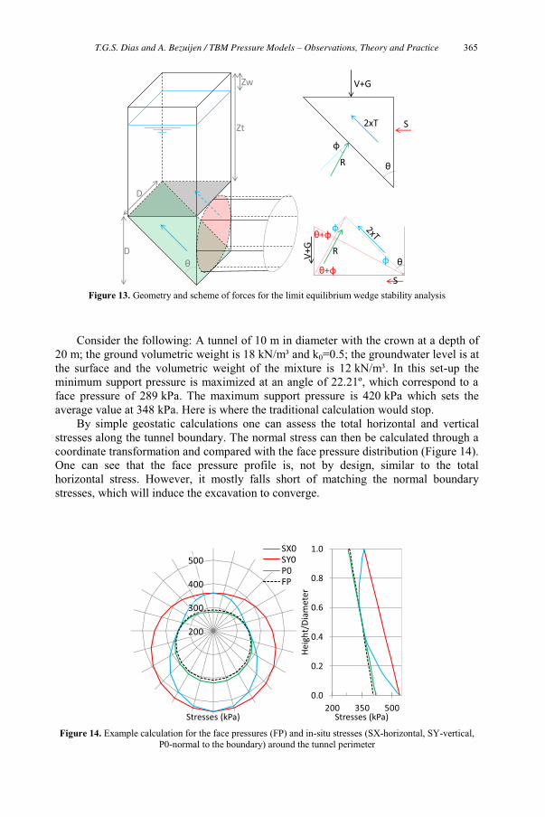
Figure 13. Geometry and scheme of forces for the limit equilibrium wedge stability analysis

Consider the following: A tunnel of 10 m in diameter with the crown at a depth of

20 m; the ground volumetric weight is 18 kN/m³ and k0=0.5; the groundwater level is at the surface and the volumetric weight of the mixture is 12 kN/m³. In this set-up the minimum support pressure is maximized at an angle of 22.21º, which correspond to a face pressure of 289 kPa. The maximum support pressure is 420 kPa which sets the average value at 348 kPa. Here is where the traditional calculation would stop.

By simple geostatic calculations one can assess the total horizontal and vertical stresses along the tunnel boundary. The normal stress can then be calculated through a coordinate transformation and compared with the face pressure distribution (Figure 14). One can see that the face pressure profile is, not by design, similar to the total horizontal stress. However, it mostly falls short of matching the normal boundary stresses, which will induce the excavation to converge.

Figure 14. Example calculation for the face pressures (FP) and in-situ stresses (SX-horizontal, SY-vertical,

P0-normal to the boundary) around the tunnel perimeter

θR

2xT

V+G

S

φ

θ

D

D

Zw

Zt

φ

φθ+φ

θ

θ+φ

V+G

S

R

200

300

400

500SX0SY0P0FP

Heig

ht/D

iam

eter

0.0

0.2

0.4

0.6

0.8

1.0

200 350 500Stresses (kPa)Stresses (kPa)


To analyze the hydraulics of the face pressure transfer, one can start by using Eq. (3) to calculate the hydraulic gradient at the tunnel face (i = ϕ0/R = 100 kPa/5 m = 2). Assuming a granular material with a permeability of 10-5 m/s and a porosity of 0.4, one can then use Eq. (4) to calculate the water penetration velocity from the mixture to the ground (v = k.i/n = 0.05 mm/s). This velocity can be assumed an upper bound to the penetration of slurry or foam bubbles, which will always have a higher viscosity than water. A regular drilling velocity of a TBM is 1 mm/s. Therefore, for this set of parameters, one can easily see that, during drilling, the supporting fluid will not be able to penetrate further than the length that is scrapped away at each rotation of the cutterhead. So, without the filter cake, increments of pore water pressure will develop ahead of the tunnel face.

The calculation can be taken further assuming the rotational speed of the cutterhead around 3 rpm and four lines of scrappers at the cutterhead. This means that the supporting fluid can penetrate 0.25 mm in the 5 s before it is scrapped away. Even a very impermeable filter cake layer, say 10-8 m/s, would only dissipate about 12 kPa of hydraulic head, transferring the other 88 kPa of hydraulic head to the soil. This pressure difference can then be set in Eq. (2) to assess how far ahead of the face this effect will be pronounced. It has been pointed out that these increments of pore water pressure can affect the minimum face support pressure. Within the limit equilibrium wedge stability framework, the system should be re-analyzed whenever there are significant increments of pore water pressure outsize the boundaries of the soil wedge. This can alter the resultant forces, especially the shear resistance on the vertical triangular walls of the wedge. In this case the water pressure at x=D.tanθ is about 41 kPa above the hydrostatic pressure, which leads a reduction of about 10 kPa in the minimum support pressure that is now set at a wedge angle of 24º.

Another consideration is the volume of water that flows out of supporting mixture. Considering the Darcy velocity of 2.10-5 m/s through the area of the tunnel face, the flow rate is about 1.57 10-3 m³/s. Imagine that a certain FIR needs to be specified to take the porosity of the saturated ground from the original 0.4 to about 0.5. If no flow is considered, an FIR=20% should suffice (Eq. (6)). However, the water flow rate represents about 5% of the initial water in the amount of muck excavated in a certain time (FWR=0.05). Therefore, a FIR=22% is necessary to compensate for the water loss (Eq. (7)).

3.2. 2nd Example – Grout Pressures

The second example presents how the assessment of the tunnelling induced displacements can be linked with a more specific calculation: the profile of grout pressures. Sections 2.3 and 2.4 highlighted how important it is to determine the grout pressures. However, the most important issue, when it comes to urban tunnelling, is and has always been how it can affect nearby structures. This potential disturbance is normally assessed through the field of induced displacements, particularly at the surface by the agency of the settlement trough.

To tackle this issue one has to understand the framework used to evaluate tunneling induced settlement and how the elements of modern TBM technologies can fit into that structure. For more than 30 years now, the traditional empirical methods [25] and analytical solutions [26] are being replaced by numerical calculations [27]. These are approximate solutions of a boundary value problem, traditionally of mechanical equilibrium, which can be obtained through, among others, the finite


element method (FEM). While the constitutive model and the mesh/domain are indispensable elements of the analysis, the main point to be discussed here are the boundary conditions.

The stress release method is the most implemented scheme to simulate the tunneling process for 2D plane-strain conditions. It applies a certain fraction of the in-situ stress as the boundary conditions of the tunnel. This was a practical tool in conventional tunneling to mimic the 3D arching effect from the face. However, for mechanized tunnels, the boundary stresses depend on the TBM operation and hold no relation to the ground in-situ stress. Several techniques have been proposed to adapt the stress release approach to the gradients of mechanized tunneling [28–30], but these methods considered constant pressures. While a considerable advance, these models do not consider the interdependence between the machine action and the soil reaction, which is the central point of argument in this paper.

To incorporate this interconnection, the models for the TBM-ground interaction should be able to generate the necessary input for the numerical analysis (the stress boundary conditions); and take in the resultant displacement field, which can be evaluated first at the tunnel boundary to re-calculate the interactions with the ground convergence, and second at the surface to determine the settlement trough. This layout can simultaneously improve how the ground deformability is considered, in comparison with the analytical formula from Eq. (11); and how the boundary conditions represent the features of mechanized tunneling.

Starting from the rheological model and the calculation spreadsheet from Section 2.3, the soil-lining gap can initially be set as the geometrical difference between the excavation radius and the lining extrados. The calculated grout pressures can then be used as boundary conditions in a FEM calculation, from which the boundary convergence can be imported back to the spreadsheet, re-evaluating the gap. This iterative process will eventually converge into the field of grout pressures and ground displacements. Such a scheme was recently implemented using an Excel spreadsheet and the FlexPDE software, a general solver for partial differential equations. The grout pressure calculated in the spreadsheet and the soil parameter are interpreted through a VBA (Visual Basic for Applications) code that writes a compatible script for the FlexPDE calculation. The script is also programmed to generate the output from the FEM calculation in a certain format. Another Excel macro then imports the FlexPDE output back into the spreadsheet to re-assess the soil-lining gap [15]. The first version of this framework was created with a linear-elastic constitutive model, but the logic can be advanced to more complex models.

This code can be set with the same parameters used in the example from Figure 9. The average results are not very different. The resultant force is 1182 kN compared to 1173 kN for the analytical model. The volume loss at the tunnel is 0.31%, while the previous model resulted in 0.38%. However, the point of remark is the possibility to simultaneously calculate the volume loss due to surface settlements, which was -0.06% in this case. A closer look in the profiles of pressures and displacements reveal a more distinct response (Figure 15). The finite element calculation resulted in larger convergence at the invert and roof of the tunnel, while it caused expansion of the tunnel springline. For both calculations the average vertical gradient of grout pressures was 14.4 kPa/m, less than the 20 kPa/m that would be expected due to the volumetric weight of the grout. On the other hand, the numerical solution resulted in higher pressures around the tunnel springline.


Figure 15. Example calculation using a finite element software for the tangential grout flow in terms of the

soil-lining gap (left) and the boundary pressures (right).

4. How do you think academy and industry could jointly benefit in your field of interest and in your country to advance design and construction practices of underground excavations?

Engineering practice derives from the will and capacity of each agent of a project (owner, contractor, designer, regulatory agencies, etc.) to maximize their interests, within generally accepted limits of conduct set by the local cultural practice. Here, the term culture should not be regarded as a historical heritage, but as a constantly evolving set of practices. Therefore, to predict changes in engineering practice is to predict human response to incentives within a certain culture. This is by no means a trivial task, and one for which the authors do not hold enough evidence for any attempt of scientific analysis. Hence, the discussions of this section will be set around personal views, which are naturally biased and unscientific, but can, hopefully, spark some arguments over the question.

The initial argument is that the industry is currently arranged in a way where a limited number of its members control most of the know-how in mechanized tunnelling and that in order to advance engineering practice, this needs to change. The ideal concept is that every agent is mainly focused on improving the project through better engineering. However, whenever there is a certain level of dominance, human agency will appeal to preserve and reinforce this state of affairs. So, one must inquiry whether the current technical level of the industry is at its optimal point or if it is being kept where it is to preserve the relative advantage of some agents, through their own momentum of production, financial and political forces or technical inclinations.

By recognizing that this is a natural tendency, one can see that it is not a matter of bad faith or something particular to one type of agent. This will happen whenever the know-how is not well distributed among the different agents of a project, at least to the

0 400 800

0

15

0

400

800

0.0

0.5

1.0

0 5 10 15 20

InitialGrout

InjectionNozzles

Soil-LiningGap (cm)

BoundaryPressure (kPa)

Heig

ht/D

iam

eter

(cm) (kPa)


extent of their attributions. This last point should be regarded with care, as among the tools to preserve a certain status quo is the control of discourse to disengage other agents from participating. Essentially, everyone needs to know the consequences of each engineering decision to achieve a project that is balanced from early design to construction and operation. For an industry with so many players, technical progress will only derive from widespread knowledge.

The unpredictability of the operation parameters of any regular drive of a TBM has become the prevalent argument to dismiss the possibility of accurate predictions for mechanized tunnels. On top of that, it is also common to conceive the TBM excavation as an automated process, analogous to an assembly line, where each step is essentially pre-determined, and where one cannot intervene. This framework results in an uneven distribution of responsibilities among the different agents for the realization of the project. The group of geotechnical design describes the geological conditions, identifies the geological risks, and possibly defines the range of face pressures. The group of structural design calculates the lining elements to resist the typical ring building forces and ground loads. However, the success of the project basically boils down to the TBM operation, which is controlled by the construction team who will consequently hold most of the know-how.

This may have several undesirable consequences for the success of the project. From the perspective of the owner or the regulatory agency, the main factor setting the success of the project, the TBM operation, is not regulated or designed in detail beforehand, specifically in terms of its consequences. In case the construction does not meet the goals of the project, there is no objective way to ascertain if the goals were unfeasible or if the operation was misguided. Afterwards, more refined methods of analyzes can lead to an explanation but this shouldn’t lead to individual accountability provided that all agents were in agreement with the previous directives, to the best of their knowledge at the time.

The idea that the execution is crucial to the success of a project cannot be challenged. This has been the case also with conventional tunneling, but that did not meant that the maximum stand-up time or the unsupported length of a tunnel were not designed, even thought they were always adjusted in the field. As the authors tried to show in this paper, there is much more to mechanized tunnelling than keeping the face pressure within the limits, especially if the stringent limitations for surface settlements, which are now common in urban areas, are to be met. This brings the discussion to the designer’s perspective.

The design team has to identify the geotechnical risks, one of which is the prediction of settlements and how the structures around the tunnel can be affected by them. A proper characterization of the ground in the design phase will enable the ground reaction to be modeled in a more representative way. However, the ground will be reacting against the actions of the TBM. If the design team is not aware of the operation parameters of the machine, they can either assume them at will or limit the design to empirical measures of volume loss and distortion. In both cases there is no connection between the design and what will actually occur in the field, the real forces during excavation and the consequent displacements. An ideal design should incorporate the operational parameters of the machine with the assessment of settlements, as discussed in Section 3.2.

Let us consider two ways in which academia could possibly help the industry to diminish the consequences of an uneven concentration of knowledge. The first is also the most obvious: education. All engineers that are now acting for the different agents


once shared the same classrooms. It is a permanent duty of academia to teach engineering students both contemporary and progressive techniques of engineering practice. But here, again, the prevalent discourse is important. If the way geotechnical engineers brand their knowledge as “classical theory” or “advanced methods” is not updated (as it hasn’t been for decades), basic education will be doing more to conform to tradition than to encourage new practices. Be that as it may, there are two normal limitations with education. One is that, continuing education programs are still struggling to reach a broad audience of engineering practitioners. In a forum to discuss these issues that was held more than 10 years ago [31], one can read: “The time pressures and financial constraints of commercial geotechnical consulting and contracting generally preclude the possibility of learning and applying newer methods and techniques.”. Another limitation is that the number of universities worldwide that provide specific courses on tunnelling is extremely small.

The tunnelling academic community is mostly concerned with applied research, which, by definition, involves the practical application of science. However, theoretical developments are regularly formulated within frameworks that are inaccessible to practitioners. While sometimes this derives from pure mathematical complexity, it is also common that the whole structure of the model is founded on concepts or parameters that are alien to the state of practice. This is direct connection with the face that some researchers ignore or are simply unaware of practical realities. On top of that is the massive number of publications available over a single topic. To mine technical value out of such extensive literature is also out of the scope of most practitioners. Therefore, the second way in which academia can help is by facilitating the link between research and practice, through more effective scientific communication and an integration of its methods with practical realities. The first point might be solved if, from time to time, the industry arranges for an academic group to filter the available knowledge for practical use, in some sort of state-of-the-art-for-practice report. The second point is more complex as it demands both sides to work together.

Take as an example the models that were discussed in this paper. Most of them derive from real constructions where the owner required a thorough investigation from a research institute to build know-how for future project. Specific instrumentation plans could capture responses that went previously undetected. From there, the theory was developed to explain the results and predict the consequences for different conditions. All of that would not have been possible without the owner’s demand and the appropriate financial resources. No university can afford to conduct a trial TBM excavation, so they need to be called upon by the industry. On the other hand, the design of specific instrumentation and monitoring plans, and the analysis of all the resultant data is outside the scope of practitioners. Therefore, the collaboration can be mutually beneficial. But for that to occur, academia must also focus on another point: the assessment of the parameters for their theoretical models. This brings the discussion back to the balance of knowledge. It is of no practical use to create a model that depends on a parameter that can only be measured in a few laboratories around the world. One can easily see that the imperative for in-situ testing present for ground characterization should be even larger for measurements to be taken during construction. Overall the conclusion is that everyone involved in a project should understand the process that is being considered, so that the engineering decisions on every level can be distilled by their consequences for every agent involved.

Referring to the “unpredictability” of field conditions, there is basically just one way out: probabilistic analysis and risk management. This has been recognized in every


field of technology, but is still part of the “advanced methods” category in engineering education. If every mechanism that has been described in this paper is ignored and lumped together in one single parameter, e.g. volume loss, it is quite expectable to obtain apparently random results. However, probabilistic methods allow the quantified variability of any parameter to be considered through any computational model, no matter how complex, to assess the variability of the results. There have been recent developments in this direction for both technical [32] and financial aspects [33]. The future might hold that not only these models will be used in the state of practice but that they will be used within probabilistic methods. Taking on the example from Figure 9, one can simulate how the variability of the ground Young’s modulus and the grout yield strength will affect the distribution of the tunnel volume loss. Assuming symmetrical triangular distributions for the input parameters, the spreadsheet can be adapted to run a Monte-Carlo simulation. Figure 16 presents the cumulative distribution functions for the input and the output. Consider an example that the aim of the project is to keep the volume loss under 0.6 %. The results indicate that the probability of failure (VL > 0.6%) is over 50% for the case in point. The whole simulation takes about 1 minute in this framework and allows for a much more elaborate design

Figure 16. Example probabilistic calculation for the tunnel volume loss at the phase of tangential grout flow.

A critical reader might argue that all that has been presented so far is an excessive

detailing effort to a problem that has already been solved. In other words, that the current state of practice can consistently achieve the technical goals set up for it. Be that as it may, the industry of underground constructions is undeniably demanding on financial and natural resources. Therefore, avoiding the disturbance limits shouldn’t justify abdicating from further optimization. Underground constructions hold a long-term comparative advantage, in terms of social, environmental and financial aspects, to regular surface structures. However, a comparative advantage does not mean that the

0.2% 0.6% 1.0%

0.5 1.0 1.5

0.0

0.2

0.4

0.6

0.8

1.0

30 40 50

Cum

ulat

ive

Prob

abili

ty

5 1 0 1Grout Yield Strength (kPa)

40Ground E (MPa)

% 0.6%Tunnel Volume Loss


amount of resources involved is not significant. Taking the example of pollution, it is estimated that the manufacture and supply of concrete tunnel lining segments generate over 1 million tons of carbon dioxide emissions every year. The use of alternative materials, currently available, could reduce that number in over 70% [34].

From a financial perspective, one can compare two of the most preeminent contemporary technological projects being developed in Europe: Crossrail and Rosetta. The first is Europe’s largest construction project, employing over 10.000 people. The future 118 km railway line will connect the central part of London (UK) with its outskirts. Ten new stations and 42 km of tunnels will be built and the construction is expected to last for about 10 years, from 2009 to 2019. The total costs are estimated in 21 billion euros. The second project is the mission of the first spacecraft to orbit and land on a comet after travelling 6.4 billion kilometers in outer space for more than 10 years, from 2004 to 2014. The mission’s goals are to investigate the physical and chemical structures of the comet and to understand its origin. This can clarify the structure of the solar system’s early days. The total mission cost was 1.4 billion euros. The scale of both projects is depicted in Figure 17.

Even though this is an eccentric association, within the context of limited public financial resources, it remarks the dimension of our industry’s responsibility when it comes to optimize our costs. There is no question that, in the short term, infrastructure projects will have a larger impact on society than space missions. However, when such a scientific progress can be funded with less than 7% of the cost of an infrastructure project, there should be a social imperative to optimize our methods and practices.

Figure 17. Scale and costs for the Rosetta Mission and the Crossrail Project.

Rosetta Mission - 10 yearsCost – 1.4 billion euros

Cross Rail Project - 10 yearsCost – 21 billion euros

37 x 10^7 km 37 km

Launch

Arrival

1

2

3

4SunEarthMarsCometOrbits1st Spin2nd Spin3rd Spin4th SpinApproach


Acknowledgements

The first author would like to acknowledge the financial support of the Brazilian Research Agency – CNPq.

References

[1] V. Guglielmetti, P. Grasso, A. Mahtab, S. Xu, eds., Mechanized tunnelling in urban areas: design methodology and construction control, Taylor & Francis, 2007.

[2] A. Bezuijen, A.M. Talmon, Processes around a TBM, Geotechnical Aspects of Underground Construction in Soft Ground - 6th International Symposium (IS-Shanghai), Shanghai, China, 2008.

[3] M. Thewes, C. Budach, A. Bezuijen, Foam conditioning in EPB tunnelling, Geotechnical Aspects of Underground Construction in Soft Ground - 7th International Symposium (IS-Rome), Rome, Italy, 2012.

[4] A. Bezuijen, J.P. Pruiksma, H.H. van Meerten, Pore pressures in front of tunnel, measurements, calculations and consequences for stability of tunnel face, International Symposium on Modern Tunneling Science and Technology, Kyoto, Japan, 2001.

[5] A. Bezuijen, P.E.L. Schaminee, J.A. Kleinjan, Additive testing for earth pressure balance shields, 12th European Conference on Soil Mechanics and Geotechnical Engineering, Amsterdam, The Netherlands, 1999.

[6] A. Bezuijen, The influence of soil permeability on the properties of a foam mixture in a TBM, Geotechnical Aspects of Underground Construction in Soft Ground - 4th International Symposium (IS-Toulouse), Toulouse, France, 2002.

[7] Z. Zizka, M. Thewes, I. Popovic, Analysis of Slurry Pressure Transfer on the Tunnel Face during Excavation, ITA World Tunnel Congress 2015 - SEE Tunnel - Promoting Tunnelling in SEE Region, Dubrovnik, Croatia, 2015.

[8] A. Bezuijen, Bentonite and grout flow around a TBM, ITA World Tunnel Congress 2007 - Underground Space – The 4th Dimension of Metropolises, Prague, Czech Republic, 2007.

[9] A. Bezuijen, The influence of grout and bentonite slurry on the process of TBM tunnelling, Geomechanik Und Tunnelbau 2 (2009), 294–303.

[10] T.G.S. Dias, A. Bezuijen, Tunnel modelling: Stress release and constitutive aspects, Geotechnical Aspects of Underground Construction in Soft Ground - 8th International Symposium (IS-Seoul), Seoul, South Korea, 2014.

[11] M.H. Mohammed, R. Pusch, S. Knutsson, G. Hellström, Rheological Properties of Cement-Based Grouts Determined by Different Techniques, Engineering 6 (2014), 217–229.

[12] J.N. Shirlaw, D.P. Richards, P. Ramond, P. Longchamp, Recent experience in automatic tail void grouting with soft ground tunnel boring machines, ITA World Tunnel Congress 2004 - Underground Space for Sustainable Urban Development, Singapore, 2004.

[13] A. Bezuijen, A.M. Talmon, F.J. Kaalberg, R. Plugge, Field measurements of grout pressures during tunnelling of the Sophia Rail Tunnel, Soils and Foundations 44 (2004), 39–48.

[14] A.M. Talmon, L. Aanen, A. Bezuijen, W.H. van der Zon, Grout pressures around a tunnel lining, International Symposium on Modern Tunneling Science and Technology, Kyoto, Japan, 2001.

[15] T.G.S. Dias, A. Bezuijen, TBM Pressure models: Calculation tools, ITA World Tunnel Congress 2015 - SEE Tunnel - Promoting Tunnelling in SEE Region, Dubrovnik, Croatia, 2015.

[16] A. Bezuijen, A.M. Talmon, Grout, the foundation of a bored tunnel, BGA International Conference on Foundations, Dundee, Scotland, 2003.

[17] L. Masini, S. Rampello, K. Soga, An Approach to Evaluate the Efficiency of Compensation Grouting, Journal of Geotechnical and Geoenvironmental Engineering 140 (2014).

[18] A. Bezuijen, W.H. van der Zon, Laboratory testing of grout properties and their influence on backfill grouting, ITA World Tunnel Congress 2005 - Underground Space Use. Analysis of the Past and Lessons for the Future, Istanbul, Turkey, 2005.

[19] A.M. Talmon, A. Bezuijen, Analytical model for the beam action of a tunnel lining during construction, International Journal for Numerical and Analytical Methods in Geomechanics 37 (2013), 181–200.

[20] R. Aime, P. Aristaghes, P. Autuori, S. Minec, 15 m diameter tunnelling under Netherlands Polders, ITA World Tunnel Congress 2004 - Underground Space for Sustainable Urban Development, Singapore, 2004.

[21] F.J. Kaalberg, J.A.T. Ruigrok, R. De Nijs, TBM face stability & excess pore presssures in close proximity of piled bridge foundations controlled with 3D FEM, Geotechnical Aspects of Underground Construction in Soft Ground - 8th International Symposium (IS-Seoul), Seoul, South Korea, 2014.


[22] M. Scheffer, T. Rahm, M. König, Simulation-Based Analysis of Surface Jobsite Logistics in Mechanized Tunneling, International Conference on Computing in Civil and Building Engineering, Orlando, USA, 2014.

[23] J. Messerli, E. Pimentel, G. Anagnostou, Experimental study into tunnel face collapse in sand, 7th International Conference on Physical Modelling in Geotechnics (ICPMG 2010), Zurich, Switzerland, 2010.

[24] G. Anagnostou, K. Kovári, The face stability of slurry-shield-driven tunnels, Tunnelling and Underground Space Technology 9 (1994), 165–174.

[25] R.B. Peck, Deep Excavations and Tunnels in Soft Ground, 7th International Conference on Soil Mechanics and Foundation Engineering, Mexico City, Mexico, 1969.

[26] C. Sagaseta, Analysis of undrained soil deformation due to ground loss, Géotechnique 37 (1987), 301–320.

[27] R.K. Rowe, K.Y. Lo, G.J. Kack, A method of estimating surface settlement above tunnels constructed in soft ground, Canadian Geotechnical Journal 20 (1983), 11–22.

[28] M.Y. Abu-Farsakh, G.Z. Voyiadjis, Computational model for the simulation of the shield tunneling process in cohesive soils, International Journal for Numerical and Analytical Methods in Geomechanics 23 (1999), 23–44.

[29] W.Q. Ding, Z.Q. Yue, L.G. Tham, H.H. Zhu, C.F. Lee, T. Hashimoto, Analysis of shield tunnel, International Journal for Numerical and Analytical Methods in Geomechanics 28 (2004), 57–91.

[30] T. Konda, J. Nagaya, T. Hashimoto, H.M. Shahin, T. Nakai, In-situ Measurement and Numerical Analysis on Tunnel Lining and Ground Behaviour due to Shield Excavation, 3rd International Conference on Computational Methods in Tunnelling and Subsurface Engineering (EURO:TUN 2013), Bochum, Germany, 2013.

[31] H.G. Poulos, P. Day, L. Valenzuela, S. Crawford, P. Mayne, M. Bolton, F. Tatsuoka, J. Koseki, Practitioner/academic Forum, 16th International Conference on Soil Mechanics & Geotechnical Engineering, Osaka, Japan, 2005.

[32] M.O. Cecílio Jr, P.I.B. Queiroz, L.P. Valenzuela, A. Negro, Probabilistic back-analysis of K0 and deformation properties of fine soils found in Line 2 of Santiago Metro, Chile, Geotechnical Aspects of Underground Construction in Soft Ground - 8th International Symposium (IS-Seoul), Seoul, Korea, 2014.

[33] P. Sander, A. Moergeli, J. Reilly, Quantitative Risk Analysis – Fallacy of the Single Number, ITA World Tunnel Congress 2015 - SEE Tunnel - Promoting Tunnelling in SEE Region, Dubrovnik, Croatia, 2015.

[34] A. Harding, M. Chappell, The case for adopting new segmental lining technologies, ITA World Tunnel Congress 2015 - SEE Tunnel - Promoting Tunnelling in SEE Region, Dubrovnik, Croatia, 2015.


Documents

Geotechnical Synergy in Buenos Aires 2015 A.O. Sfriso et ... · additives, and is removed from the chamber mechanically, through a screw conveyor. In slurry pressure balance (SPB)