Embed Size (px)
Citation preview

GEOTECHNIC
ENGINEERING-1
LABORATORY MANUAL
DEPARTMENT OF CIVILENGINEERING
JORHAT ENGINEERING COLLEGE
JORHAT, ASSAM-785007

DEPARTMENT OF CIVIL ENGINEERING, JORHAT ENGINEERING COLLEGE
SOIL MECHANICS LABORATORY
DETERMINATION OF FIELD DENSITY OF SOIL BY CORE CUTTER METHOD
THEORY:
Core cutter method is used for finding field density of cohesive/clayey soils placed as fill.
It is rapid method conducted on field. It cannot be applied to coarse grained soil as the penetration
of core cutter becomes difficult due to increased resistance at the tip of core cutter leading to
damage to core cutter.
The density or unit weight (γ) is defined as the total weight of soil mass (w) per unit of its
total volume (v). Here the weight and volume of soil comprise the whole soil mass. The voids in
the soil may be filled with both water and air or only air consequently the soil may be wet, dry or
saturated. Mathematically,
Density, γ = 𝑤
𝑣
The water content w, also called the moisture content is defined as the ratio of weight of water
(ww) to the weight of solids (ws) in a given mass of soil. Mathematically,
Water content, w = 𝑊𝑤
𝑊𝑠×100%
The dry density (γd) is the weight of soil solids per unit of total volume of the soil mass.
Mathematically,
Dry density, γd = γ
1+𝑤
It may be noted here that the field density always refers to the dry density because the wet
density of soil at location varies from season to season and based on the fluctuations of the local
water table level and surface water.

APPARATUS REQUIRED:
1. Cylindrical core cutter of steel
2. Steel rammer
3. Steel dolly
4. Palette knife
5. Steel rule
6. Straight edge
7. Balance
8. Container for water content determination
9. Thermostatically controlled oven
Fig 1: Core cutter apparatus
PROCEDURE:
1. Measures the inside dimensions, then find the volume and weight of the core cutter.
2. Clean areas of about 30 cm × 30 cm in the field, put the dolly on the top and drive the
assembly into the soil.
3. Dig out the container from the soil and trim off both the sides of the cutter.
4. Weight the cutter, fall of soil and calculate the final density for water content
determination.
5. Weight a small empty container (w1).

6. Keep some representative specimen of soil in the container and weight it again (w2).
7. Keep the container in the oven for 24 hours and then weight it again (w3).
8. Find the water content and repeat the procedure from step 5 to step 8 as required.
OBSERVATION TABLE:
Determination of field density of soil:
1. Weight of core cutter mould = ___________
2. Weight of core cutter mould + wet soil = _________
3. Weight of wet soil, W= __________
4. Length of the mould = __________
5. Inner diameter of mould = __________
6. Volume of mould, V = _________
7. Field density (γ) = 𝑊
𝑉
Water content determination:
Container
No.
Weight of
container, (w1)
(gm)
Weight of container
+ wet soil (w2)
(gm)
Weight of container
+ dry soil (w3)
(gm)
Water content
(w)
Water content, w = (𝑤2−𝑤3)
(𝑤3−𝑤1)
Dry density, γd = 𝛾
1+𝑤
CALCULATION:
PRECAUTIONS:
1. Core cutter method of determining the field density of soil is only suitable for fine grained
soil (silts and clay). This is because collection of undisturbed soil sample from a coarse
grained soil is difficult hence the field properties, including unit weight, cannot be
maintained in a core sample.
2. Core cutter should be driven into the ground till the steel dolly penetrates into the ground
halfway only so as to avoid compaction of the soil in the core.
3. Before lifting the core cutter, soil around the cutter should be removed to minimise the
disturbance
REMARK:
QUESTIONS:
1. What do you understand by dry, wet, saturated and submerged density of soil? Explain.
2. Out of various types of densities, which one of them is maximum and which is minimum?
Explain.
3. What are the field problems, where density of soil needs to be determined?
4. In what type of soil do we prefer core cutter method of determining the field density?
Why?
5. In fully saturated soils, what is the degree of saturation?
6. What is the degree of saturation in oven dry soils?

DEPARTMENT OF CIVIL ENGINEERING, JORHAT ENGINEERING COLLEGE
SOIL MECHANICS LABORATORY
DETERMINATION OF FIELD DENSITY BY SAND REPLACEMENT METHOD
THEORY:
In core cutter method, the field density of soil is obtained from direct measurements.
However, it is not always possible (particularly in case of sandy soil) to obtain a core sample. In
such situations, the sand replacement method is employed to determine the field density.
In sand replacement method, a small cylindrical pit is excavated and weight of the soil
excavated from the pit is measured. By measuring the weight of sand required to fill the pit and
knowing its density, the volume of the pit is calculated. Knowing the weight of soil excavated
from the pit and the volume of the pit, the density of the soil calculated. Therefore in this
experiment, there are two stages:
Calibration of sand density
Measurement of soil
The dry density of the excavated soil is determined as:
γd = 𝛾
1+𝑤
Where, γ = Density of the excavated soil
W = water content
Fig 1: sand replacement method

APPARATUS REQUIRED:
1. Sand pouring cylinder
2. Calibrating container
3. Metal tray with a central hole
4. Dry sand ( passing through 600μm sieve )
5. Balance
6. Scoop
7. Chisel and hammer
8. Oven
9. Big tray and small tray
PROCEDURE:
Stage 1: Calibration of Sand Density
1. The volume of the calibrating container is determined from the measured dimensions of
the container.
2. The sand pouring cylinder is filled with sand within 10mm of its top. The mass of the
cylinder is determined (M1).
3. The sand pouring cylinder is placed vertically on the calibrating container. The shutter is
open to allow the sand run out from the cylinder. The shutter is close when there is no
further movement of the sand in the cylinder.
4. The sand pouring cylinder is lifted from the calibrating container and weighed (M3).
5. Again, the sand pouring cylinder is filled with sand within 10mm of its top.
6. The sand pouring cylinder is place over a plane surface, such as the big try. The shutter is
open. The sand filled the cone of the cylinder. The shutter is closed when no further
movement of sand takes place.
7. The sand pouring cylinder is removed. The sand left on the big tray is collected. The mass
of sand (M2) that had filled the cone is thus determined by weighing the collected sand.
8. The dry density of sand is determined.

Stage 2: Measurement of Soil Density
1. An area of about 450mm square on the surface of the soil is exposed and trimmed using a
chisel and hammer.
2. The metal tray with a hole is place on the level surface.
3. The soil through the central hole of the tray is excavated by using the hole in the tray and
the depth of the excavated hole should be about 150mm.
4. All the excavated soil in a metal container is collected and the mass of the soil is
determined from it. The excavated soil is placed in to the oven for 24 hours to determine
the water content.
5. The metal tray is removed from the excavated hole.
6. The sand pouring cylinder is filled within 10mm of its top. The mass of the cylinder (M4) is
determined.
7. The sand pouring cylinder is placed over the excavated hole. The sand is allowed to run out
of the cylinder by opening the shutter. The shutter is closed when the hole is completely
filled and no further of movement of sand id observe.
8. The sand pouring cylinder is remove from the filled hole. The mass of the cylinder (M5) is
determined.
9. A representative sample of the excavated soil is taken. Water content and dry density are
determined.
OBSERVATION TABLE:
Stage 1: Calibration of Sand Density:
Volume of calibrating container(m3), v = πr
2h
Mass of cylinder + cap (kg)
Mass of cylinder + sand + cap (Before pouring), M1 (kg)
Mass of cylinder + sand + cap (After pouring), M3 (kg)
Mass of big tray (kg)
Mass of big tray + sand (kg)
Mass of sand, M2 (kg)

Bulk density of the sand = Weight of sand filled in the calibrationg container
Volume of the calibrating container
γ = M/V = 𝑀1−𝑀3−𝑀2
𝑉
Stage 2: Measurement of Soil Density:
Volume of calibrating container(m3), v = πr
2h
Mass of cylinder + cap (kg)
Mass of cylinder + sand + cap (Before pouring), M4 (kg)
Mass of cylinder + sand + cap (After pouring), M5 (kg)
Mass of small tray (kg)
Mass of small tray + excavated soil (before heating) (kg)
Mass of excavated soil, Mw kg
Mass of small tray + excavated soil ( after heating) (kg)
Mass of sand, M2 (kg)
Bulk density of the soil = weight of the excavated soil
weight of the sand in the hole× bulk density of sand
ρb = 𝑀𝑤
𝑀𝑏 × ρa = 𝑀𝑤
𝑀4−𝑀5−𝑀2×ρa
PRECAUTIONS:
1. If for any reason, it is necessary to excavate the pit to a depth other than 12 cm, the
standard calibrating can should be replaced by one with an internal height same as the
depth of the pit to be made in the ground.
2. Care should be taken in excavating the pit, so that it is not enlarged by levering as this will
result in lower density being recorded.
3. No loose material should be left in the pit.
4. There should be no vibration during the test.

5. It should not be forgotten to remove the tray, before placing the sand pouting cylinder over
the pit.
QUESTIONS:
1. In what type of soils is sand replacement method of determining the field density is
preferred? Why?
2. Why do you prefer to keep the depth of the pit equal to the height of the calibrating
cylinder?

DEPARTMENT OF CIVIL ENGINEERING, JORHAT ENGINEERING COLLEGE
SOIL MECHANICS LABORATORY
GRAIN SIZE ANALYSIS BY SIEVE AND HYDROMETER ANALYSIS
DRY METHOD: SIEVE ANALYSIS
THEORY:
Soil gradation or sieve analysis is used in the engineering classification of soil, particularly
coarse grained soil. It is the distribution of particle sizes expressed as a percent of the total dry
weight. Gradation is determined by passing the material through a series of sieves stacked with
progressively smaller openings from top to bottom and weighing the material retained on each
sieve. As per IS classification of soil, soil is classified as coarse grained and fine grained soil. Soils
having particle size coarser than 0.075mm size is termed as coarse grained soil.
Besides the particle size, the distribution of different sizes is needed to classify the soil as
either well graded or poorly graded. The two parameters i.e. uniformity coefficient, Cu and
coefficient of curvature, Cc is obtained from the grain size analysis tests are utilized in the
classification of soil. Uniformity coefficient, Cu is a measure of particle size range and is given by
the ratio of D60 and D10 i.e.
Uniformity coefficient, Cu = 𝐷60
𝐷10
Coefficient of curvature, Cc= (𝐷30 )2
𝐷60 𝑥 𝐷10
For a uniformly graded soil, Cu is nearly 1. For a well graded soil, Cc must be between 1 to
3 and in addition Cu must be greater than 4 for gravel and 6 for sand.
APPARATUS REQUIRED:
1. A series of sieve sets ranging from 4.75mm to 75μm (4.75mm, 2.00mm, 1.00mm, 425μm,
212μm, 150μm, 75μm)
2. Balance sensitive to ± 0.01g
3. Thermostatically controlled oven

PROCEDURE:
1. Take 500gm of the soil sample from disturbed representative sample.
2. Conduct sieve analysis using a set of standard sieves as given in the data sheet.
3. The sieving is done by hand or by mechanical sieve shaker for 10 minutes.
4. Then weighed the material retained on each sieve.
5. The percentage retained on each sieve is calculated on the basis of the total weight of the
soil sample taken.
6. From these results the percentage passing through each of the sieves is calculated.
7. Draw the grain size curve for the soil in the semi-logarithmic graph provided.
Fig 1: Particle size distribution curve
PRECAUTIONS:
1. Clean the sieves set so that no soil particles were struck in them
2. While weighing put the sieve with soil sample on the balance in a concentric position.
3. Check the electric connection of the sieve shaker before conducting the test.
0
10
20
30
40
50
60
70
80
90
100
0.01 0.1 1 10
% F
iner
Particle size (mm)

PRESENTATION OF DATA
TABLE1: SIEVE ANALYSIS
Sieve size Weight
retained in
gms
%
Retained
Cumulative
weight
retained in
gms
Cumulative
% finer
4.75 mm
2.36 mm
1.18 mm
600 µ
300 µ
150 µ
75 µ
pan
* Percent passing=100-cumulative percent retained.
From Grain Size Distribution Curve:
D10= ____ mm
D30= ___ mm
D60= __ mm
Cu =
Cc =

QUESTIONS:
1. What is the purpose of sieve analysis?
2. Why do you classify soil?
3. What do you understand by uniformly graded and well graded soils?
4. What is meant by gap graded soil?
5. What do you understand by GW, GP, GM, GC, SW, SP, SM, SC in soil classification?
WET SIEVING AND HYDROMETER ANALYSIS:
THEORY:
Wet sieving is done to determine the distribution of particle size finer than 75 micron. The
percentage of sand, silt and clay in the inorganic fraction of soil is measured in this procedure. The
method is based on Stoke’s law governing the rate of sedimentation of particles suspended in water
and it is done by using density hydrometer.
APPARATUS REQUIRED:
1. Glass cylinders of 1000-ml capacity
2. Thermometer
3. Hydrometer
4. Electric mixer with dispersing cup
5. Balance sensitive to ± 0.01g
6. Stop watch & Beaker
RE-AGENTS REQUIRED:
Dispersing solution-4% (Dissolve 5 g of sodium hexa-metaphosphate in de-ionized water of 125
ml)
PROCEDURE:
1. Take about 50g in case of clayey soil and 100g in case of sandy soil and weigh it correctly to
0.1g.
2. In case the soil contains considerable amount of organic matter or calcium compounds, pre-
treatment of the soil with Hydrogen Peroxide or Hydrochloric acid may be necessary. In case

of soils containing less than 20 percent of the above substances pre-treatment shall be
avoided.
3. To the soil thus treated, add 100 cc of sodium hexa-metaphosphate solution and warm it
gently for 10 minutes and transfer the contents to the cup of the mechanical mixer using a jet
of distilled water to wash all the traces of the soil.
4. Stir the soil suspension for about 15 minutes.
5. Transfer the suspension to the Hydrometer jar and make up the volume exactly to 1000 cc by
adding distilled water.
6. Take another Hydrometer jar with 1000cc distilled water to store the hydrometer in between
consecutive readings of the soil suspension to be recorded. Note the specific gravity readings
and the temperature T°C of the water occasionally.
7. Mix the soil suspension roughly, by placing the palm of the right hand over the open end and
holding the bottom of the jar with the left hand turning the jar upside down and back. When
the jar is upside down be sure no soil is tuck to the base of the graduated jar.
8. Immediately after shaking, place the Hydrometer jar on the table and start the stopwatch.
Insert the Hydrometer into the suspension carefully and take Hydrometer readings at the total
elapsed times of ¼, ½, 1 and 2 minutes.
9. After 2 minutes reading, remove the Hydrometer and transfer it to the distilled water jar and
repeat step no-8. Normally a pair of the same readings should be obtained before proceeding
further.
10. Take the subsequent hydrometer readings at elapsed timings of 4, 9, 16, 25, 36, 49, 60
minutes and every one hour thereafter. Each time a reading is taken remove the hydrometer
from the suspension and keep it in the jar containing distilled water. Care should be taken
when the Hydrometer recorded to see that the Hydrometer is at rest without any movement.
As time elapses, because of the fall of the solid particles the density of the fluid suspension
decreases reading, which should be checked as a guard against possible error in readings of
the Hydrometer.
11. Continue recording operation of the Hydrometer readings until the hydrometer reads 1000
approximately.
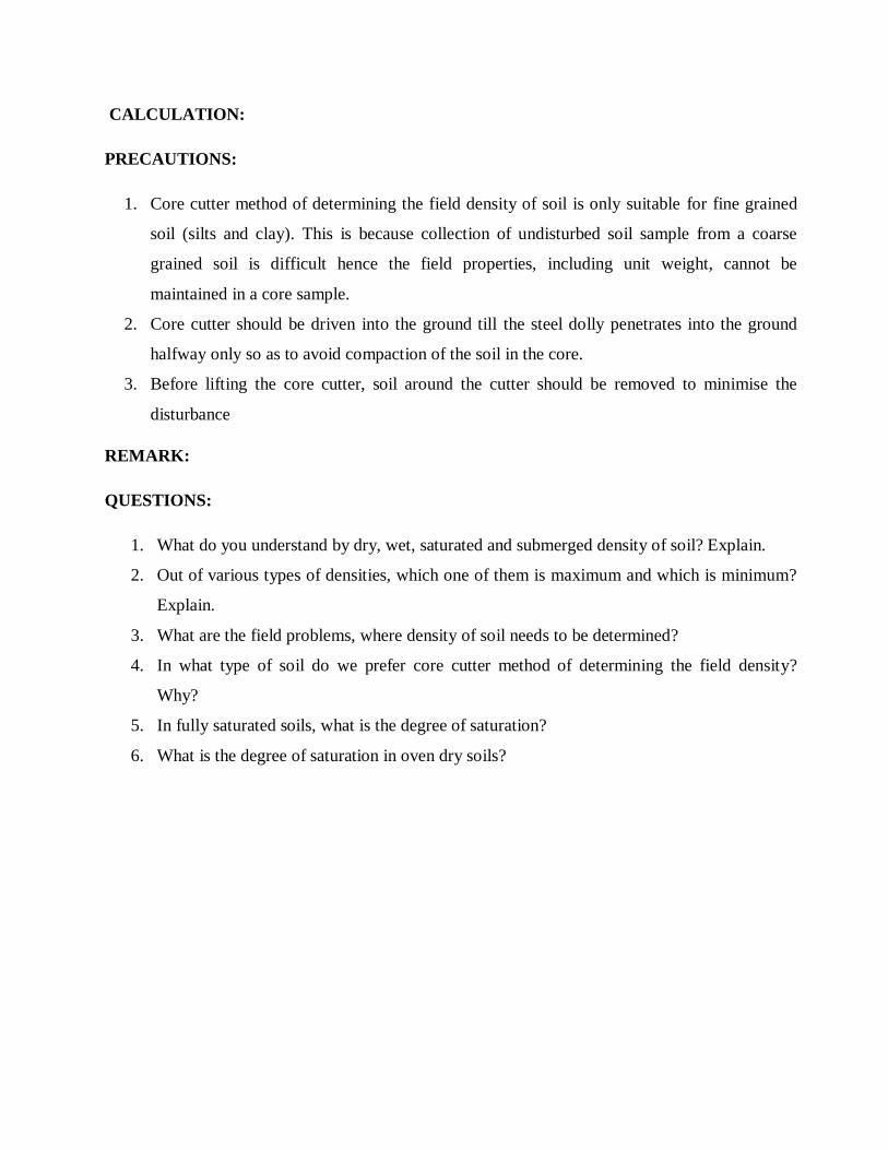
CALIBRATION OF THE HYDROMETER
The hydrometer shall be calibrated to determine its true depth in terms of the hydrometer reading
(see Fig-2) in the following steps:
Fig 2: Hydrometer calibration
1. Determine the volume of the hydrometer bulb, VR. This may be determined in following way:
By measuring the volume of water displaced. Fill a 1000-cc graduate with water to
approximately 700 cc. Observe and record the reading of the water level. Insert the
hydrometer and again observe and record the reading. The difference in these two readings
equals the volume of the bulb plus the part of the stem that is submerged. The error due to
inclusion of this latter quantity is so small that it may be neglected for practical purposes.
2. Determine the area, A, of the graduate in which the hydrometer is to be used by measuring the
distance between two graduations. The area, A, is equal to the volume included between the
graduations divided by the measured distance.
3. Measure and record the distances from the lowest calibration mark on the stem of the
hydrometer to each of the other major calibration marks, R.
4. Measure and record the distance from the neck of the bulb to the lowest calibration mark. The
distance, H1, corresponding to a reading, R, equals the sum of the two distances measured in
steps (3) and (4).

5. Measure the distance from the neck to the tip of the bulb. Record this as h, the height of the
bulb. The distance, h/2, locates the center of volume of a symmetrical bulb. If a
nonsymmetrical bulb is used, the center of volume can be determined with sufficient accuracy
by projecting the shape of the bulb on a sheet of paper and locating the center of gravity of
this projected area.
6. Compute the true distances, HR, corresponding to each of the major calibration marks, R,
from the formula:
HR = H1 + ½ [h – (VR/A)]
7. Plot the curve expressing the relation between HR and R as shown in Figure 3. The relation is
essentially a straight line for hydrometers having a streamlined shape.
Fig 3: Typical hydrometer calibration chart
CALCULATION:
If the temperature during the experiment is constant, then the the following formula can be
used to calculate the diameter of the soil particles
D2 = K HR/t
Where
t = time in minutes
D = diameter of soil particle in mm

K = 30η/(G-γw)
The percentage finer N may be obtained from
N% = G*V/ ((G-1)*W) * (r – rw)*100
Where
V = Volume of soil suspension (1000 cc)
W = weight of dry soil taken for the test
r = Hydrometer reading in distilled water
rw = Hydrometer readings in soil suspension
G = Specific gravity of soil particles
Since V = 1000 cc, the above equation may be conveniently represented as follows:
N% = K1 (Rh1 – 1000) * 100
Where
K1 = G/ (G-1) * (100/W)
Rh1 = Hydrometer reading = Rh + Cm – Cd ± Ct
Where,
Rh = actually observed hydrometer reading (upper meniscus)
Cm = the meniscus correction (i.e. 0.5)
Ct = Correction for temperature (positive if the test temperature is more than the temperature at
which the hydrometer is calibrated and vice versa) (see table-1)
Cd = Correction for dispersing agent. This is determined as mentioned below.
The addition of a dispersing agent to the soil suspension results in an increase in density of
the liquid and necessitates a correction to the observed hydrometer reading. The correction factor,
Cd, is determined by adding to a 1000-ml graduate partially filled with distilled or demineralized
water the amount of dispersing agent to be used for the particular test, adding additional distilled
water to the 1000-ml mark, then inserting a hydrometer and observing the reading. The correction
factor, Cd is equal to the difference between this reading and the hydrometer reading in pure
distilled or demineralized water.

Table-1 Temperature Correction (Ct) for Hydrometer Analysis
Temp in 0C Ct Temp in
0C Ct
20.0 Nil 27 0.00150
20.5 0.00009 27.5 0.00163
21 0.00017 28 0.00178
21.5 0.00027 28.5 0.00191
22 0.00037 29 0.00206
22.5 0.00049 29.5 0.00219
23 0.00058 30 0.00232
23.5 0.00068 30.5 0.00247
24 0.00081 31 0.00262
24.5 0.00092 31.5 0.00278
25 0.00102 32 0.00291
25.5 0.00116 32.5 0.00320
26 0.00127 33 0.00350
26.5 0.00139 33.5 0.00380
Table - 2 Variation of L with Hydrometer Reading
Hydrom
eter
Reading
L
(cm)
Hydrom
eter
Reading
L
(cm)
Hydrom
eter
Reading
L
(cm)
Hydrom
eter
Reading
L
(cm)
0
1
2
3
4
5
6
16.3
16.1
16.0
15.8
15.6
15.5
15.3
13
14
15
16
17
18
19
14.2
14
13.8
13.7
13.5
13.6
13.2
26
27
28
29
30
31
32
12
11.9
11.7
11.5
11.4
11.2
11.1
39
40
41
42
43
44
45
9.9
9.7
9.6
9.4
9.2
9.1
8.9

7
8
9
10
11
12
15.2
15
14.8
14.7
14.5
14.3
20
21
22
23
24
25
13
12.9
12.7
12.5
12.4
12.2
33
34
35
36
37
38
10.9
10.7
10.6
10.4
10.2
10.1
46
47
48
49
50
51
8.8
8.6
8.4
8.3
8.1
7.9
PRESENTATION OF DATA:
1. Sample No:
2. Hydrometer No. =
3. Cross-sectional area of the jar, A=
4. Soil’s specific gravity oil (Gs) =
5. Dispersing agent correction (Cd) =
6. Weight of soil for sieve analysis (W) =
7. Weight of oven dried soil in suspension (WS) =
8. Temperature correction (Ct) =
9. Weight passing from 0.075 mm sieve (Wf) =
10. Meniscus correction (Cm) =
Elapsed
time ‘t’
(in min)
Hydrometer
Reading
(Rh)
R’h= (Rh + Cm) Corrected
hydrometer
reading,
Rh1= R’h +
(Ct – Cd)
L, Effective
Depth
[table 2]
K L/T (L in
cm & T in
min)
√L/T Particle size
D=K√L/T
(in mm)
Percent
Finer N'
%
% Finer
on the
total wt.
N
N' % =( GS × Rh1 × 100)/(GS –1) × WS
Where GS = Specific Gravity of Soil

WS = Dry Wt. of Soil sample
N % = Wf × N' %
Present results by plotting particle size vs. percent finer on a semi-logarithmic sheet.
PRECAUTIONS:
1. Before each insertion of hydrometer, check that the stem is dry.
2. Practice insertion of hydrometer and recording of reading before starting the experiment.
3. Check that the temperature in sedimentation jar and control jar are same during the entire
period of test.
QUESTIONS:
1. When do you go for hydrometer analysis?
2. What are the corrections that are to be applied to the observed readings of the hydrometer?
3. What is stoke’s law? How does it help in hydrometer analysis?

DEPARTMENT OF CIVIL ENGINEERING, JORHAT ENGINEERING COLLEGE
SOIL MECHANICS LABORATORY
DETERMINATION OF LIQUID LIMIT, PLASTIC LIMIT AND SHRINKAGE LIMIT OF
SOIL
a) LIQUID LIMIT TEST
THEORY:
It is the arbitrary limit between liquid and plastic stages of consistencies of soil, as
defined by Atterberg. This is the limiting moisture content at which the cohesive soil passes
from plastic state to liquid state. Experimentally, Liquid Limit is the moisture content at which
the groove, formed by a standard tool into the sample of soil taken in the standard cup, closes
for 10 mm on being given 25 blows in a standard manner.
Liquid limit is significant to know the stress history and general properties of the soil
met with construction. From the results of liquid limit, the compression index may be
estimated. If the natural moisture content of soil is closer to liquid limit, the soil can be
considered as soft. If the moisture content is far lesser than liquid limit, the soil is brittle and
stiffer.
APPARATUS REQUIRED:
1. Balance
2. Casagrande’s Liquid limit device,
3. Grooving tool (Spatula)
4. Mixing dish.
5. Thermostatically controlled Oven
6. Squeeze bottle.
7.
PROCEDURE:
1. Take 250 gm of oven-dried soil, passed through 425 µm sieve, into an evaporating dish.
Add distilled water into the soil and mix it thoroughly to form uniform paste. (The paste

should have a consistency that would require 30 to 35 drops of cup to cause closer of
standard groove for sufficient length.)
2. Place a portion of the paste in the cup of Liquid Limit device and spread it with a few
strokes of spatula.
3. Trim it to a depth of 1 cm at the point of maximum thickness and return excess of soil to
the dish.
4. Using the spatula cut a groove along the centre line of soil pat in the cup, so that
clean sharp groove of proper dimension (11 mm wide at top, 2 mm at bottom, and 8 mm
deep) is formed.
5. Lift and drop the cup by turning crank at the rate of two revolutions per second until the
two halves of soil cake come in contact with each other for a length of about 13 mm by
flow only, and record the number of blows, N.
6. Take a representative portion of soil from the cup for moisture content determination.
7. Repeat the test with different moisture contents at least five more times for blows between
15 and 35
OBSERVATIONS:
Details of the sample:
Natural moisture content: Room temperature:
Determination
Number
1 2 3 4 5 6
Container number
Weight of container (w1)
Weight of container + wet soil (w2)
Weight of container + dry soil (w3)
Weight of water (Ww=w2-w3)
Weight of dry soil (Ws=w3-w1)

CALCULATIONS:
Plot the relationship between water content (on y-axis) and number of blows (on x-axis) on
semi-log graph. The curve obtained is called flow curve. The moisture content corresponding
to 25 drops (blows) as read from the represents liquid limit. It is usually expressed to the
nearest whole number.
Liquid limit, WL = Water content corresponding to 25 blows,
(From semi log- graph of water content Vs. No. of blows)
Fig 1:.No. of blows vs. water content
Flow index, If= (W2-W1) / log (N1/N2)
= slope of the flow curve
b) PLASTIC LIMIT TEST
THEORY:
Plastic limit is the arbitrary limit between semi-solid and plastic stages of
consistencies of soil, as defined by Atterberg. It represents the moisture content between
these stages. Experimentally, Plastic Limit (PL) is determined by rolling out a thread of the
fine portion of a soil on a flat, non-porous surface. The plastic limit is defined as the moisture
content where the thread attains a diameter of 3 mm (about 1/8 inch) and simultaneously
Moisture content (%) = (Ww/Ws)
No. of blows

surface cracks appear on it, without the thread being broken or buckled. A soil is considered
non-plastic if a thread cannot be rolled out down to 3 mm at any moisture content.
APPARATUS REQUIRED:
1. Porcelain dish,
2. Squeeze bottle and spatula,
3. Balance of capacity 200gm and sensitive to 0.01 gm,
4. Ground glass plate for rolling and specimen,
5. Containers to determine the moisture content,
6. Oven thermostatically controlled with interior of non-corroding material to
maintain the temperature around 105° and 110°C
PROCEDURE:
1. Put 20 gm of air-dried soil, passed through 425 μm sieve (In accordance with I.S.
2720: part-1), into an evaporating dish. Add distilled water into the soil and mix it
thoroughly to form uniform paste (the soil paste should be plastic enough to be easily
moulded with fingers).
2. Prepare several ellipsoidal shaped soil masses by squeezing the soil between your
fingers. Take one of the soil masses and roll it on the glass plate using your figures.
The pressure of rolling should be just enough to make thread of uniform diameter
throughout its length. The rate of rolling shall be between 60 to 90 strokes per min.
3. Continue rolling until you get the thread diameter of 3 mm.
4. If the thread does not crumble at a diameter of 3 mm, kneed the soil together
to a uniform mass and re-roll.
5. Continue the process until the thread crumbles when the diameter is 3 mm.
6. Collect the pieces of the crumbled thread for moisture content determination.
(Prepare threads at least with 10gm of soil for water content measurement).
7. Repeat the test at least 3 times and take the average of the results calculated to the nearest
whole number.
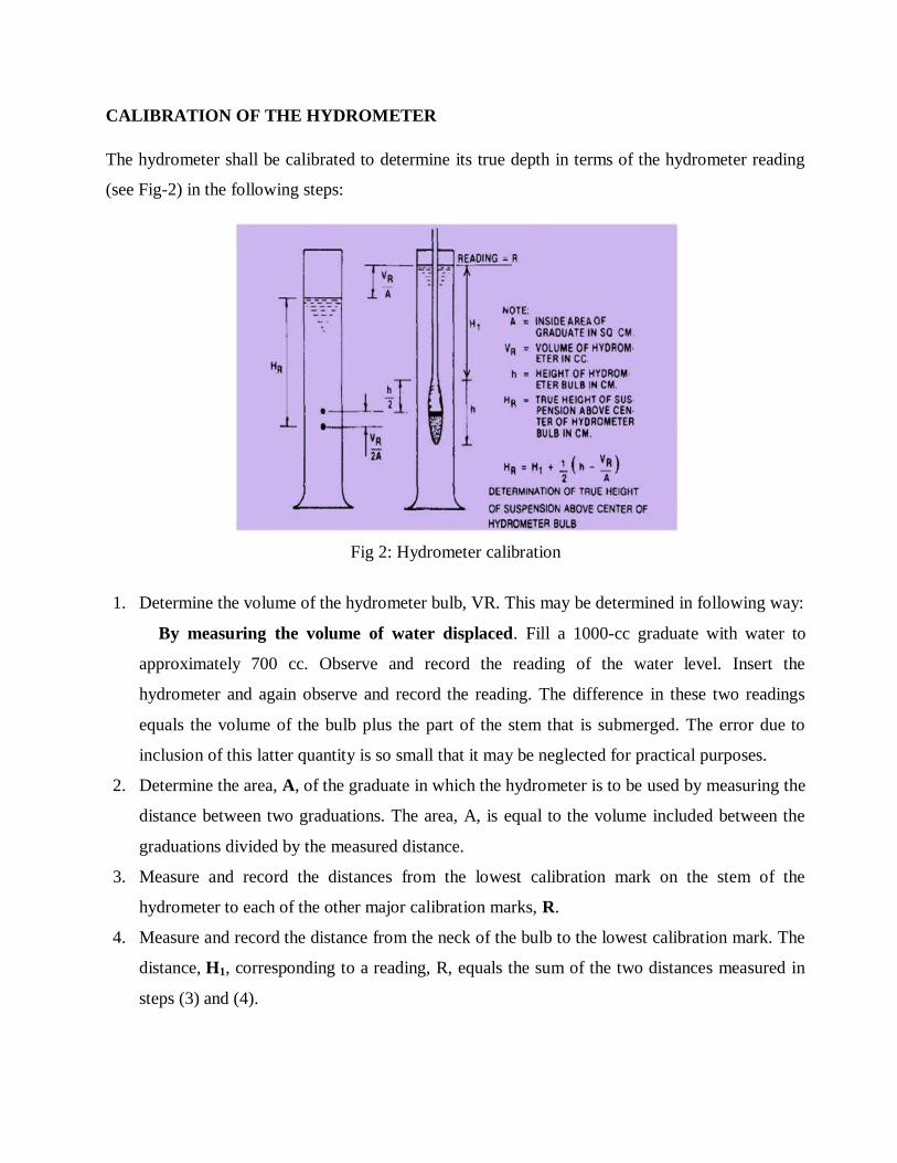
PRESENTATION OF DATA
DISCUSSION:
1. The difference between in moisture content between liquid and plastic limit is termed as
Plasticity Index. Mathematically
Plasticity Index (Ip) = (LL - PL)
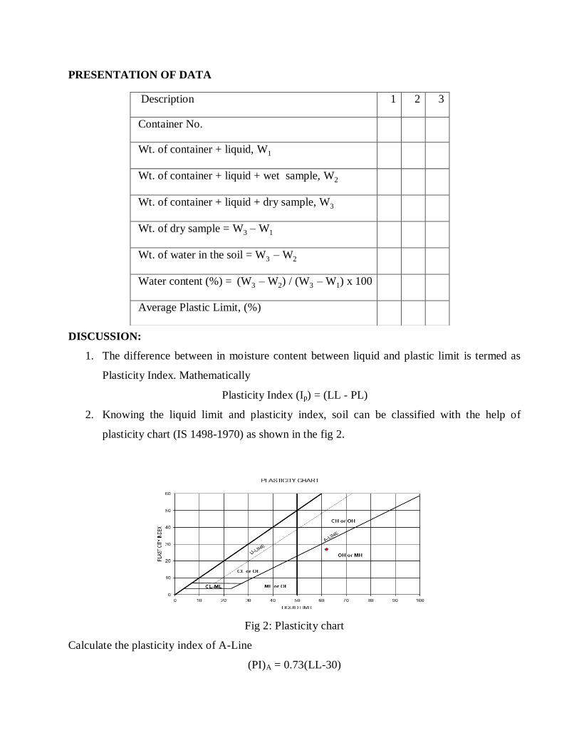
2. Knowing the liquid limit and plasticity index, soil can be classified with the help of
plasticity chart (IS 1498-1970) as shown in the fig 2.
Fig 2: Plasticity chart
Calculate the plasticity index of A-Line
(PI)A = 0.73(LL-30)
Description 1 2 3
Container No.
Wt. of container + liquid, W1
Wt. of container + liquid + wet sample, W2
Wt. of container + liquid + dry sample, W3
Wt. of dry sample = W3 – W1
Wt. of water in the soil = W3 – W2
Water content (%) = (W3 – W2) / (W3 – W1) x 100
Average Plastic Limit, (%)

Where LL is the liquid limit
If PI > (PI)A, the soil is clay
If PI < (PI)A, the soil is silt
If LL = 0-35, low compressibility
If LL = 35-50 medium compressibility
If LL > 50 high compressibility
In plasticity chart the following symbols are used:
CL= clay of low compressibility
CI= clay of medium or intermediate compressibility
CH= clay of high compressibility
ML= silt of low compressibility
MI= silt of medium or intermediate compressibility
MH= silt of high compressibility
OL= organic soil of low compressibility
OI= organic soil of medium or intermediate compressibility
OH= organic soil of high compressibility
3. Toughness Index = plasticity index ,Ip
flow index ,If
PRECAUTIONS:
1. Soil used for liquid limit and plastic limit determinations should not be oven dried prior to
testing.
2. In liquid limit test, the groove should be closed by the flow of soil and not by slippage
between the soil and the cup.
3. After mixing the water to the soil sample, sufficient times should be given to permeate the
water throughout the soil mass.
4. Wet soil taken in the container for moisture content determination should not be left open
in the air, the container with soil sample should either be placed in descicator pr
immediately be weighed.

QUESTIONS
1. How the plastic limit is defined to determine it in the laboratory?
2. How does oven dried soil sample effect the value of plastic limit?
c) SHRINKAGE LIMIT TEST:
THEORY:
Shrinkage limit is defined as the maximum water content at which a reduction in water
content will not cause a decrease in the volume of a soil mass. It is the minimum water
content at which a soil can still be completely saturated. It is the state which acts as boundary
between semi solid state and plastic state.
APPARATUS REQUIRED:
1. Evaporating Dish of Porcelain,
2. Spatula and Straight Edge,
3. Balance-Sensitive to 0.01 g minimum.
4. Shrinkage Dish - Circular, porcelain or non-corroding metal dish,
5. Glass cup. 50-55 mm in diameter and 25 mm in height,
6. Glass plates - Two, 75 mm one plate of plain glass and the other prongs,
7. 425 µ sieve
8. Balance, sensitive to 0.1 to 0.01g
9. Thermostatically controlled Oven,
10. Wash bottle containing distilled water,
11. Graduate- glass with capacity of 25 ml and mercury.
PROCEDURE:
Preparation of soil paste
1. Take about 100 gm of soil sample from a thoroughly mixed portion of the material
passing through 425 μm Sieve. Place about 30 gm of the above soil sample in the

evaporating dish and thoroughly mixed with distilled water and make a creamy
paste. (Use water content slightly higher than the liquid limit.)
Filling the shrinkage dish
2. Coat the inside of the shrinkage dish with a thin layer of silicon grease or Vaseline to
prevent the soil sticking to the dish.
3. Fill the dish in three layers by placing approximately 1/3 rd of the amount of wet soil
with the help of spatula. Tap the dish gently on a firm base until the soil flows over the
edges and no apparent air bubbles exist. Repeat this process for 2nd and 3rd layers also
till the dish is completely filled with the wet soil. Strike off the excess soil and make
the top of the dish smooth. Wipe off all the soil adhering to the outside of the dish.
4. Weigh immediately the dish with wet soil and record the weight.
5. Air- dry the wet soil cake for 6 to 8 hrs, until the colour of the pat turns from dark to
light. Then oven-dry the cake at 1050C to 110
0C say about 12 to 16 hours.
6. Remove the dried disk of the soil from oven. Cool it in a desiccators. Then obtain the
weight of the dish with dry sample. 7. Determine the weight of the empty dish and
record.
7. Determine the volume of shrinkage dish which is evidently equal to volume of the wet soil
as follows:
8. Place the shrinkage dish in an evaporating dish and fill the dish with mercury till it
overflows slightly. Press it with plain glass plate firmly on its top to remove excess
mercury. Pour the mercury from the shrinkage dish into a measuring jar and find the
shrinkage dish volume directly. Record this volume as the volume of wet soil pat.
Volume of the Dry Soil Pat
9. Determine the volume of dry soil pat by removing the pat from the shrinkage dish and
immersing it in the glass cup full of mercury in the following manner.
Place the glass cup in a larger one and fill the glass cup to overflowing with
mercury. Remove the excess mercury by covering the cup with glass plate with
prongs and pressing it. See that no air bubbles are entrapped. Wipe out the outside of
the glass cup to remove the adhering mercury. Then, place it in another larger
dish, which is, clean and empty carefully.

Place the dry soil pat on the mercury .Submerge the pat which is floating with the
pronged glass plate which is again made flush with top of the cup. The mercury
spills over into the larger plate. Pour the mercury that is displaced by the soil pat into
the measuring jar and find the volume of the soil pat directly.
TABULATION AND RESULTS:
PRECAUTION:
1. Do not touch the mercury with gold ring
QUESTION
1. Define shrinkage limit.
Sl. No Determination No. 1 2 3
1 Wt. of container in gm,W1
2 Wt. of container + wet soil pat in gm,W2
3 Wt. of container + dry soil pat in gm,W3
4 Wt. of oven dry soil pat, W0 in gm = (W3-W1)
5 Wt. of water in gm = (W2-W3)
6 Moisture content (%), W = (W2-W3)/ (W3-W1)×100
7 Volume of wet soil pat (V), in cm
8 Volume of dry soil pat (Vd) in cm3 = (Wm)/ (Gm) By
mercury displacement method
a. Weight of displaced mercury in gm (Wm)
b. Specific gravity of the mercury (Gm)
9 Shrinkage limit (WS) = [W – {(V-Vd) x /Wo}] x 100
10 Shrinkage ratio (R) = {(V1-Vd)/Vd}×(W-Ws)×100

DEPARTMENT OF CIVIL ENGINEERING, JORHAT ENGINEERING COLLEGE
SOIL MECHANICS LABORATORY
PERMEABILITY TEST BY FALLING HEAD METHOD
THEORY:
The property of the soil which permits water to percolate through its continuously
connected voids is called its permeability. The rate of flow under laminar flow conditions through
a unit cross sectional area of porous medium under unit hydraulic gradient is defined as coefficient
of permeability, K. It has the velocity dimensions.
Factors affecting the coefficient of permeability can be studied from the equation
K = Cd2γw/ η (e
3/(1+e))
Where,
K = coefficient of permeability
C = constant
d = diameter of the soil grains
γw = unit weight of water
η = viscosity of fluid (water)
e = void ratio of soil
Viscosity and unit weight of water depend upon temperature, hence coefficient of
permeability is affected by the climatic conditions. Constant C depends upon the arrangement and
shape of soil grains and voids. The coefficient of permeability may be determined both in the
laboratory and field.
The test may be conducted both above and below water table but is considered more
accurate below water table. It is applicable for strata in which the hole below the casing pipe can
stand and has low permeability; otherwise the rate of fall of the head may be so high that it may be
difficult to measure.

PREPARATION OF THE SPECIMEN
The preparation of the specimen for this test is important. There are two types of specimen,
the undisturbed soil sample and the disturbed or made up soil sample.
A. UNDISTURBED SOIL SPECIMEN
It is prepared as follows:
1. Note down-sample no., borehole no., depth at which sample is taken.
2. Remove the protective cover (wax) from the sampling tube.
3. Place the sampling tube in the sample extract or and push the plunger to get a cylindrical shaped
specimen not larger than 85 mm diameter and height equal to that of the mould.
4. This specimen is placed centrally over the drainage disc of base plate.
5. The annular space in between the mould and specimen is filled with an impervious material like
cement slurry to block the side leakage of the specimen.
6. Protect the porous disc when cement slurry is poured.
7. Compact the slurry with a small tamper.
8. The drainage cap is also fixed over the top of the mould.
9. The specimen is now ready for test.
B. DISTURBED SPECIMEN
The disturbed specimen can be prepared by static compaction or by dynamic compaction.
(a)Preparation of statically compacted (disturbed) specimen.
1. Take 800 to 1000 gms of representative soil and mix with water to O.M.C determined by I.S
Light Compaction test. Then leave the mix for 24 hours in an airtight container.
2. for the given volume (V) of the mould, calculate the mass (M) of the soil mixso as to give the
desired dry density (γd), using the following expression:
M = γd (1 + w) V. take the mass of the soil accurate to 1 g.
3. Now, assemble the permeameter for static compaction. Attach the 3 cm collar to the bottom end
of 0.3 liters mould and the 2 cm collar to the top end. Support the mould assembly over 2.5 cm end
plug, with 2.5 cm collar resting on the split collar kept around the 2.5 cm- end plug. The inside of
the 0.3 lit. Mould is lightly greased.
4. Put the weighed soil into the mould. Insert the top 3 cm end plug into the top collar, tamping the
soil with hand.

5. Keep, now the entire assembly on a compressive machine and remove the split collar. Apply the
compressive force till the flange of both end plugs touch the corresponding collars. Maintain this
load for 1 min and then release it.
6. Then remove the top 3 cm plug and collar place a filter paper on fine wire mesh on the top of the
specimen and fix the perforated base plate.
7. Turn the mould assembly upside down and remove the 2.5 cm end plug and collar. Place the top
perforated plate on the top of the soil specimen and fix the top cap on it, after inserting the seating
gasket.
8. Now the specimen is ready for test.
(B) Preparation of Dynamically Compacted Disturbed sample:
1. Take 800 to 1000 gms of representative soil and mix it with water to get O.M.C, if necessary.
Have the mix in airtight container for 24 hours.
2. Assemble the permeameter for dynamic compaction. Grease the inside of the mould and place it
upside down on the dynamic compaction base. Weigh the assembly correct to a gram (w). Put the
3 cm collar to the other end.
3. Now, compact the wet soil in 2 layers with 15 blows to each layer with a 2.5 kg dynamic tool.
Remove the collar and then trim off the excess. Weigh the mould assembly with the soil (W2).
4. Place the filter paper or fine wore mesh on the top of the soil specimen and fix the perforated
base plate on it.
5. Turn the assembly upside down and remove the compaction plate. Insert the sealing gasket and
place the top perforated plate on the top of soil specimen. And fix the top cap.
6. Now, the specimen is ready for test.
APPARATUS REQUIRED:
1. Permeameter with its accessories:
2. Standard soil specimen,
3. Desired water,
4. Balance to weigh up to 1 gm,
5. I.S sieves 4.75 mm and 2 mm,
6. Mixing pan,
7. Stop watch,
8. Measuring jar,

9. Meter scale,
10. Thermometer,
11. Container for water,
12. Trimming knife
PROCEDURE:
1. Prepare the soil specimen as specified.
2. Saturated the specimen preferably by using desired water.
3. Assemble the Permeameter (The Permeameter is made of non-corrodible material with a
capacity of 1000 ml, with an 0.1 mm) in the bottom tank and filled the tank with water.0.1 mm
and effective height of 127.3internal diameter of 100
4. Inlet nozzle of the mould is then connected to the stand pipe and allowed the water to flow until
steady flow is obtained.
5. Note down the time interval‘t’ for a fall of head in the stand pipe ‘h’.
6. Repeat step 5 three times to determine t’ for the same head.
For cohesive soils falling head method is suitable.
OBSERVATION & RECORDING:
Sample No. …………………
Molding water content: ………………..
Dry Density: ……………….
Specific Gravity: ………………………..
Void ratio ………………….
Sl.
No.
Description 1 st
set
2 nd
set
3 rd
set
1. Area of stand pipe (dia. 5 cm) a (cm2)
2. Cross sectional area of soil specimen A (cm2 )
3. Length of soil specimen L (cm)
4. Initial reading of stand pipe (h1) h1 (cm)
5. Final reading of stand pipe (h2) h2 (cm)

6.
Time
T (sec)
7.
Test temperature T (°C)
8. Coefficient of permeability at …….. °C, k =
2.303.a.L.(log10 (h1/h2) )/ (A.t)
k (cm/sec)
9. Average Permeability, kt kt (cm/sec)
10. Coefficient of permeability at 27°C :
k27 = kt 𝑡
27
k27 (cm/sec)
Variation of ηt / η27
Temperature 15 16 17 18 19 20 21 22
ηt / η27 1.336 1.301 1.268 1.237 1.206 1.177 1.149 1.122
Temperature 23 24 25 26 27 28 29 30
ηt / η27 1.096 1.071 1.046 1.023 1 0.979 0.958 0.938
DISCUSSIONS:
1. Coefficient of permeability is used to assess drainage characteristics of soil, to predict rate of
settlement founded on soil bed.
2. Magnitudes of permeability:
High permeability: k > 10-1 cm/sec
Medium permeability: k 10-1 cm/sec
Low permeability: k < 10-1 cm/sec
3. General values of permeability for different types of soils are given below:
a. Gravel: 10-2 to 1 cm/sec
b. Sand: 1 to 10-3 cm/sec
c. Silt: 10-3 to 10-6 cm/sec
d. Clay: less than 10-6 cm/sec
e. Fly Ash: 1× 10 -4 to 5× 10 -4 cm/sec
PRECAUTIONS:
1. There should be no volume change in the soil during test

2. There should be no compressible air present in the voids of soil i.e. soil should be
completely saturated during test
3. The flow should be laminar and in a steady state condition during test.
QUESTIONS:
1. What is meant by permeability and coefficient of permeability of soil?
2. What is the effect of temperature on coefficient of permeability?
3. For fine grained soil which method of permeability test is suitable?

DEPARTMENT OF CIVIL ENGINEERING, JORHAT ENGINEERING COLLEGE
SOIL MECHANICS LABORATORY
CONSOLIDATION TEST
THEORY:
When a compressive load is applied to soil mass, a decrease in its volume takes place, the
decrease in volume of soil mass under stress is known as compression and the property of soil
mass having its tendency to decrease in volume under pressure is known as compressibility. In a
saturated soil mass having its void filled with incompressible water, decrease in volume or
compression can take place when water is expelled out of the voids. Such a compression resulting
from a long time static load and the consequent escape of pore water is termed as consolidation.
Then the load is applied on the saturated voids, the soil mass, the entire load is carried by pore
water in the beginning. As the water begins escaping from the voids, hydrostatic pressure in water
gets gradually dissipated and the load is shifted to the soil particles which increases effective stress
on them, as a result the soil mass decrease in volume. The rate of escape of water depends on the
permeability of the soil.
Fig 1: Consolidometer
APPARATUS REQUIRED:
1. Consolidometer consisting essentially;
a) A ring diameter of 60 mm and height of 20 mm.
b) Two porous plates of stones of silicon carbide, aluminium oxide or porous metal.
c) Guide ring.
d) Outer ring.

e) Water jacket with base.
f) Pressure Pad.
g) Rubber basket.
2. Loading device consisting of frame, lever system, loading yoke dial gauge fixing device
and weights.
3. Dial gauge (accuracy of 0.002 mm), thermostatically controlled oven, stopwatch, sample
extractor, balance, soil trimming tools, spatula, filter papers, sample containers.
SAMPLE PREPARATION:
1. Undisturbed Sample:
a. From the sample tube, eject the sample into the consolidation ring. The sample should
project about one cm from the outer ring.
b. Trim the sample smooth and flush with top and bottom of the ring by using wire saw.
c. Clean the ring from outside and keep it ready for weighing.
2. Remolded sample:
a. Choose the density and water content at which sample has to be compacted from the
moisture-density curve, and
b. Calculate the quantity of soil and water required to mix and compact.
c. Compact the specimen in compaction mould in three layers using the standard rammers.
d. Eject the specimen from the mould using the sample extractor
PROCEDURE:
1. Saturate two porous stones either by boiling in distilled water about 15 minute or by
keeping them submerged in the distilled water for 4 to 8 hrs. Fittings of the Consolidometer
which is to be enclosed shall be moistened.
2. Assemble the Consolidometer, with the soil specimen and porous stones at top and bottom
of specimen, and providing a filter paper between the soil specimen and porous stone
3. Position the pressure pad centrally on the top porous stone. Mount the mould assembly on
the loading frame, and center it such that the load applied is axial. Make sure that the
porous stone and pressure pad are not touching the walls of mould on their sides

4. Position the dial gauge to measure the vertical compression of the specimen. The dial
gauge holder should be set so that the dial gauge is in the beginning of its releases run, and
also allowing sufficient margin for the swelling of the soil, if any.
5. Fill the mould with water and apply an initial load to the assembly. The magnitude of this
load should be chosen by trial, such that there is no swelling. It should be not less than 50
g/cm2 for ordinary soils & 25 g/cm
2 for very soft soils. The load should be allowed to stand
until there is no change in dial gauge readings for two consecutive hours or for a maximum
of 24 hours
6. Note the final dial reading under the initial load. Apply first load of intensity 0.1 kg/cm2
(Approx.) and start the stopwatch simultaneously. Record the dial gauge readings at
various time intervals. The dial gauge readings are taken until 90% consolidation is
reached. Primary consolidation is gradually reached within 24 hrs.
7. At the end of the period, specified above take the dial reading and time reading. Double the
load intensity and take the dial readings at various time intervals. Repeat this procedure for
successive load increments. The usual loading intensity is as follows (Approx.): 0.1, 0.2,
0.5, 1, 2, 4 and 8 kg/cm2
8. After the last loading is completed, reduce the load to 1⁄4 of the value of the last load and
allow it to stand for 24 hrs. Reduce the load further in steps of 1⁄4 the previous intensity till
an intensity of 0.1 kg/cm2 is reached. Take the final reading of the dial gauge
9. Reduce the load to the initial load, keep it for 24 hrs and note the final readings of the dial
gauge.
10. Quickly dismantle the specimen assembly and remove the excess water on the soil
specimen in oven, note its dry weight.
OBSERVATION AND READING:
Table I: Data Sheet for Consolidation Test: Time-Displacement Relationship
Ring Dimensions: Diameter: ____________ Area: _____________ Height: _____________
Initial Data: Specimen Ht.___________ Specific Gravity of Soil: ___________
Mass of top porous stone + cap + ball bearing: __________

Table II: Data Sheet for Consolidation Test: Pressure-Voids Ratio
Applied
Pressure
Final
dial
reading
Change
in
Specimen
Height
Final
Specimen
Height
Height
of
Solids
Height
Of
Voids
Void
Ratio
Average
Height
during
Consoli
dation
Fitting
Time,
t90
Coefficient
of
Consolida-
tion,Cv
0
0.1
0.2
0.5
1.0
Pressure
Intensity
(Kg/cm2)
0.1 0.2
0.5 1 2 4 8
Time(min)
0
0.25
1
2
4
8
15
30
1hr
2hrs
4hrs
8hrs
24hrs

2.0
4.0
8.0
2.0
0.5
0.1
CALCULATIONS:
1. Height of solids (H S) is calculated from the equation
H S= W S/(G S.γ w. A)
2. Void ratio. Voids ratio at the end of various pressures are calculated from equation
e = (H – H S)/H S
3. Coefficient of consolidation. The Coefficient of consolidation at each pressure increment is
calculated by using the following equations:
i. C v= 0.197 d2/t50 (Log fitting method)
ii. C v= 0.848 d2/t90 (Square fitting method)
In the log fitting method, a plot is made between dial readings and logarithmic of time, and
the time corresponding to 50% consolidation is determined. In the square root fitting method, a
plot is made between dial readings and square root of time, and the time corresponding to90%
consolidation is determined. The values of C v are recorded in Table II.
4. Compression Index. To determine the compression index, a plot of voids ratio (e) Vs log (t) is
made. The virgin compression curve would be a straight line and the slope of this line would give
the compression index Cc.
5. Coefficient of compressibility. It is calculated as follows
a v= 0.435 Cc/ (Avg. pressure) for the increment
where,
Cc= Coefficient of compressibility

6. Coefficient of permeability. It is calculated as follows
k = C v.a v.γ w/ (1+e o).
GRAPHS:
1. Dial reading VS log of time or
2. Dial reading VS square root of time.
3. Voids ratio VS log ζ’ (average pressure for the increment).
E - log (t) curve
Fig 2:Settlement versus time curve for 50 kPa pressure using Taylor method (sq rt time)
Settlement

Fig 3: Settlement versus time curve for 50 kPa pressure using Casagrande method (log time)
PRECAUTIONS:
1. While preparing the specimen, attempts has to be made to have the soil strata orientated in
the same direction in the consolidation apparatus.
2. During trimming care should be taken in handling the soil specimen with least pressure.
3. Smaller increments of sequential loading have to be adopted for soft soils

QUESTIONS:
1. What are the units of coefficient of consolidation?
2. What do you mean by single drainage and double drainage?
3. Why are consolidation tests done mainly on clay?
4. What do you understand by elastic settlement, primary settlement and secondary
settlement?

JORHAT ENGINEERING COLLEGE, DEPARTMENT OF CIVIL
ENGINEERING SOIL MECHANICS LABORATORY
SWELLING INDEX TEST
THEORY:
Swelling and shrinking of soil leads to distress in the substructure resulting in failure of
foundation. Swelling of soils exerts upward pressure on the foundation. The amount of pressure
exerted by the soil depends on the amount of increase in volume. The swelling pressure test
provides the actual pressure that the soil can exert on the foundation which can be directly
incorporated in design calculations. However, the procedure to estimate the swelling pressure is
time consuming and it needs specialized equipment. To identify a soil as expansive a quick test is
designed which is based on the measurement of volume change of soil when it comes in contact
with water. The increase in volume as a percentage of initial volume of soil is referred as free swell
index of soil.
Fig 1: two graduated cylinders containing soil specimen and filled with distilled
water and kerosene respectively to measure free swell index
APPARATUS:
1. 425 micron IS sieve
2. Graduated glass cylinders (100 ml. capacity 2no.s)
3. Glass rod for stirring
4. Sensitive balance (accuracy 0.01 g)
5. kerosene

PROCEDURE:
1. Two representative dried soil samples are taken each of 10 gms passing through 425
micron sieve.
2. Each soil sample is poured into each of the two glass graduated cylinders of 100 ml.
capacity.
3. One cylinder is filled with kerosene and the other with distilled water upto 100 ml mark.
4. The entrapped air is removed in cylinder by gentle shaking with a glass rod.
5. The samples are allowed to settle in both cylinders.
6. Sufficient time not less than 24 hours shall be allowed for soil sample to attain equilibrium
state of volume without any further change in volume of the soils.
7. Read out the level of soil in the kerosene-filled graduated cylinder (Vk). Kerosene, being
non-polar liquid, does not cause swelling of soil.
8. Read the level of soil in that distilled water-filled graduated cylinder (Vd)
DETERMINATION OF FREE SWELL INDEX OF SOIL:
Determination
No. Measuring cylinder no Reading after 24 hours Free swell
index
Kerosene Distilled
water
Kerosene Distilled
water
CALCULATIONS:
Free Swell Index, (%) =( (Vd-Vk)/Vk)×100
Vd = Volume of the soil specimen read from the graduated cylinder containing
distilled water.
Vk = Volume of the soil specimen read from the graduated cylinder containing
kerosene.

Note:
1. The level of the soil in kerosene graduated cylinder is read as original volume of the soil
samples, kerosene being non polar liquid does not cause swelling of the soil.
2. The level of the soil in distilled water cylinders is read as free swell level. The
individual and mean results to the nearest second decimal are recorded.
PRECAUTION:
1. In the case of highly expensive soils such as Sodium Betonite, the sample size may be 5
grams or alternatively a cylinder of 250 ml capacity for 10 grams of sample may be
used.
RESULTS:
The free swell index is expressed as a percentage to two significant figures.

DEPARTMENT OF CIVIL ENGINEERING, JORHAT ENGINEERING COLLEGE
SOIL MECHANICS LABORATORY
DETERMINATION OF OPTIMUM MOISTURE CONTENT (OMC) AND MAXIMUM
DRY DENSITY FOR A SOIL BY STANDARD PROCTOR COMPACTION TEST
THEORY:
In geotechnical engineering, soil compaction is the process in which a stress applied to a
soil causes densification as air is displaced from the pores between the soil grains. It is an
instantaneous process and always takes place in partially saturated soil (three phase system).the
degree of compaction of a soil is measured in terms of its dry density. The degree of compaction
mainly depends upon its moisture content during compaction, compaction energy and the type of
soil. For a given compaction energy, every soil attains the maximum dry density at a particular
water content which is known as optimum moisture content. The standard proctor compaction test
is a laboratory method of experimentally determining the optimum moisture content at which a
given soil type will become most dense and achieve its maximum dry density.
APPARATUS REQUIRED:
1. Proctor mould having a capacity of 1000 cc, with an internal diameter of 10.2 cm and a height
of 11.6 cm. The mould shall have a detachable collar assembly and a detachable base plate.
2. Rammer: A mechanical operated metal rammer having a 5 cm diameter face and a weight of 2.6
kg. The rammer shall be equipped with a suitable arrangement to control the height of drop to a
free fall of 31 cm.
3. Sample extruder
4. Mixing tools such as mixing pan, spoon, towel, and spatula.
5. A balance of 15 kg capacity
6. Sensitive balance
7. Straight edge
8. Graduated cylinder
9. Moisture tins
10. Thermostatically controlled oven
PROCEDURE:
1. Measure the inside dimensions of the mould and find the volume and weight of the mould.
2. Take a representative oven-dried sample, approximately 3 kg in the given pan passing through
4.75 mm I.S. sieve. Thoroughly mix the sample with sufficient water to dampen it with
approximate water content of about 7 % for sand and 10% for clay of weight of the soil sample.
3. Fix the collar and base plate. Place the soil in the Proctor mould and compact it in 3 layers
giving 25 blows per layer with the 2.6 kg rammer falling through a height of 310 mm. The
blows shall be distributed uniformly over the surface of each layer.
4. Remove the collar; trim the compacted soil even with the top of mould using a straight edge and
weigh.
5. Find out the bulk density (γ) and keep a small representative sample in the oven for water
content determination.
6. Find out the moisture content and dry density.
7. Add water in sufficient amounts to increase the moisture content of the soil sample by one or
two percentage of water and repeat the above procedure for each increment of water added.
Continue this series of determination until there is either a decrease or no change in the wet unit
weight of the compacted soil.
8. Plot a curve of dry density as ordinate and water content as abscissa and fine out the optimum
moisture content and maximum dry density.
CALCULATIONS:
Length of the mould =
Diameter of the mould =
Volume of the mould =
Empty weight of the mould =

Sl.
No.
Water
added
(ml)
Wt. of
mould
with
soil
Water Content Determination Wt.
of
soil
(gm)
Bulk
density
(γ)
gm/cc
Dry
density(γd)
gm/cc
Empty wt.
of
container
(gm)
W1
Wt. of
container
+ soil
(gm)
W2
Wt. of
container
+ dry soil
(gm)
W3
W%
1
2
3
4
5
Fig1: OMC vs MDD graph
RESULTS:
From graph,
Optimum moisture content, OMC (%) =
Maximum dry density, MDD (gm/cc) =
PRECAUTION:
1. Adequate period (about 15 minutes for clay soils and 5 minutes for sandy soils) is allowed
after mixing the water ad before compacting into the mould.
2. The blows should be uniformly distributed over the surface of each layer.

3. Each layer of compacted soil is scored with spatula before placing the soil for the
succeeding layer.
QUESTIONS:
1. What is compaction of soil? Why it is done?
2. Differentiate between compaction and consolidation of soil?
3. What is maximum dry density and optimum moisture content?
4. What are the field applications of compaction test?

DEPARTMENT OF CIVIL ENGINEERING, JORHAT ENGINEERING COLLEGE
SOIL MECHANICS LABORATORY
DIRECT SHEAR TEST
THEORY- CONCEPT:
The concept of direct shear is simple and mostly recommended for granular soils,
sometimes on soils containing some cohesive soil content. The cohesive soils have issues
regarding controlling the strain rates to drained or undrained loading. In granular soils, loading can
always assumed to be drained. A schematic diagram of shear box shows that soil sample is placed
in a square box which is split into upper and lower halves. Lower section is fixed and upper section
is pushed or pulled horizontally relative to other section; thus forcing the soil sample to shear/fail
along the horizontal plane separating two halves. Under a specific Normal force, the Shear force is
increased from zero until the sample is fully sheared. The relationship of Normal stress and Shear
stress at failure gives the failure envelope of the soil and provide the shear strength parameters
(cohesion and internal friction angle).
Fig 1: typical set up for a direct shear test

APPARATUS REQUIRED:
10. Direct shear box apparatus, and Loading frame (motor attached).
11. Dial gauge, Proving ring, Balance to weigh up to 200 g.
12. Tamper, Straight edge, Aluminum container, Spatula.
PROCEDURE:
9. Check the inner dimension of the soil container, and put the parts of the soil container
together.
10. Calculate the volume of the container. Weigh the container.
11. Place the soil in smooth layers (approximately 10 mm thick). If a dense sample is desired tamp
the soil.
12. Weigh the soil container, and find the weight of soil. Calculate the density of soil.
13. Plane the top surface of soil, and put the upper grating stone and loading block on top of soil.
14. Measure the thickness of soil specimen.
7. Apply the desired normal load and Remove the shear pin.
8. Attach the dial gauge which measures the change of volume.
9. Record the initial reading of the dial gauge and calibration values.
10. Check all adjustments to see that there is no connection between two parts except sand/soil.
11. Start the motor. Take the reading of the shear force and volume change till failure.
12. Add corresponding normal stress and continue the experiment till failure
13. Record carefully all the readings. Set the dial gauges zero, before starting the experiment
DATA CALCULATION SHEET FOR DIRECT SHEAR TEST:
1. Proving ring constant :- ______ kg/division
2. Dial gauge division: ______mm/division
3. Size of the shear box : 6cm x 6cm x 3cm

Sl.
No.
Displacement
(cm)
Corrected
Area
(cm2)
Shear
Force
(kg)
Shear
Stress
(kg/cm2)
1
2
3
4
5
6
7
CALCULATIONS:
1. Shear stress (η) on the horizontal failure plane are calculated as η = S/A; Where S is
shear force. A is the cross sectional area of the sample, which decreases slightly with the
horizontal deformations.
2. Corrected area (Acorr) needs to be calculated for calculating the shear stress at failure. Acorr
= A0 (1- δ
3), where δ is horizontal displacement due to shear force applied on specimen. A0 is
the initial area of the soil specimen.
3. i. Shear Stress = (Proving ring reading x Proving ring constant)/A
ii. Horizontal displacement = Horizontal dial gauge reading x Least count of horizontal dial
gauge
iii. Vertical displacement = Vertical dial gauge reading x Least count of vertical dial gauge
4. Shear stress at failure needs to be calculated for all three tests performed at three different
normal stresses to plot the failure envelope.
5. Plot the stress- horizontal displacement readings and obtain the maximum shear stress and its
corresponding longitudinal displacement.

6. Plot the applied normal stress as the abscissa and the maximum shear stress as the ordinate.
The slope of the straight line so obtained would give the angle of shearing resistance and the
vertical intercept of the line will give the cohesion intercept.
Fig 2: Stress- horizontal displacement graph
Fig 3: Applied normal stress vs. shear stress graph
GENERAL REMARKS:
1. In the shear box test, the specimen is not failing along its weakest plane but along a
predetermined or induced failure plane i.e. horizontal plane separating the two halves of the
shear box. This is the main drawback of this test. Moreover, during loading, the state of stress
cannot be evaluated. It can be evaluated only at failure condition i.e.
Mohr’s circle can be drawn at the failure condition only. Also failure is progressive.

2. Direct shear test is simple and faster to operate. As thinner specimens are used in shear box,
they facilitate drainage of pore water from a saturated sample in less time. This test is also
useful to study friction between two materials – one material in lower half of box and another
material in the upper half of box.
3. The angle of shearing resistance of sands depends on state of compaction, coarseness of
grains, particle shape and roughness of grain surface and grading. It varies between 28o
(uniformly graded sands with round grains in very loose state) to 46o
(well graded sand with
angular grains in dense state).
4. The volume change in sandy soil is a complex phenomenon depending on gradation, particle
shape, state and type of packing, orientation of principal planes, principal stress ratio, stress
history, magnitude of minor principal stress, type of apparatus, test procedure, method of
preparing specimen etc. In general loose sands expand and dense sands contract in volume on
shearing. There is a void ratio at which either expansion contraction in volume takes place.
This void ratio is called critical void ratio. Expansion or contraction can be inferred from the
movement of vertical dial gauge during shearing.
5. The friction between sand particles is due to sliding and rolling friction and interlocking
action.
The ultimate values of shear parameter for both loose sand and dense sand
approximately attain the same value so, if angle of friction value is calculated at ultimate
stage, slight disturbance in density during sampling and preparation of test specimens will
not have much effect.
PRECAUTIONS:
1. Before starting the test, the upper half of the box should be brought in contact of the
proving ring assembly.
2. Before subjecting the specimen to shear, the fixing pins should be taken out.
3. The rate of strain should be constant throughout the test.
4. For drained test, the porous stone should be de-aired and saturated by boiling.’
QUESTIONS:
1. What is shear strength of soil? Explain.
2. What are the shear strength parameters? Are these constant or variable for a given soil?

3. What are undrained, consolidated undrained and drained test? When are they performed?
4. What are the other laboratory and field methods to determine shear strength of soils?

DEPARTMENT OF CIVIL ENGINEERING, JORHAT ENGINEERING COLLEGE
SOIL MECHANICS LABORATORY
UNCONFINED COMPRESSIVE STRENGTH OF SOIL SPECIMEN BY USING
UNCONFINED COMPRESSION TEST
THEORY:
An Unconfined compression test is also known as uniaxial compression tests, is special
case of a triaxial test, where confining pressure is zero. UC test does not require the sophisticated
triaxial setup and is simpler and quicker test to perform as compared to triaxial test. In this test, a
cylinder of soil without lateral support is tested to failure in simple compression, at a constant rate
of strain. The compressive load per unit area required to fail the specimen as called unconfined
compressive strength of the soil.
Fig 1: compressive strength test apparatus
APPARATUS REQUIRED:
1. Loading frame with constant rate of movement.
2. Proving ring of 0.01 kg sensitivity for soft soils; 0.05 kg for stiff soils.
3. Soil trimmer, evaporating dish (Aluminium container).

4. Frictionless end plates (Perspex plate with silicon grease coating)of required diameter (diameter
of the plate is selected according to the diameter of the sample).
5. Dial gauge (0.01 mm accuracy), Dial gauge (sensitivity 0.01mm)
6. Vernier callipers
7. Balance of capacity 200 g and sensitivity to weigh 0.01 g.
8. Thermostatically controlled oven with interior of non-corroding material.
9. Soil sample of required dimensions (diameter and height)
10. Sample extractor and split sampler.
PREPARATION OF SPECIMEN:
In this test, a cylinder of soil without lateral support is tested to failure in simple compression,
at a constant rate of strain. The compressive load per unit area required to fail the specimen is
called unconfined compressive strength of the soil.
A. Undisturbed specimen
1. The sample number, bore-hole number and the depth at which the sample was taken are noted
down
2. The protective cover (paraffin wax) from the sampling tube is removed
3. The sampling tube extractor has to be placed and the plunger is pushed till a small length of
sample moves out.
4. The projected sample is trimmed using a wire saw, and the plunger is pushed until a 75mm
long sample comes out.
5. This sample is cut-out carefully and it is held on the split sampler so that it does not fall.
6. About 10 to 15 g of soil is taken from the tube for water content determination.
7. The container number is noted and the net weight of the sample and the container is taken.
8. The diameter at top is, middle, and bottom of the sample are measured. The average has to be
found and recorded.
9. The length and weight of the sample are measured and recorded.

B. Remoulded sample
1. For the desired water content and the dry density, the weight of the dry soil WS required for
preparing a specimen of required dimensions (diameter and height) is calculated.
2. Required quantity of water Ww to this soil is added
3. The soil is mixed thoroughly with water
4. The wet soil is placed in a tight thick polythene bag in a humidity chamber.
5. After 24 hours, the soil is taken from the humidity chamber and the soil is placed in a constant
volume mould, of required dimensions (equivalent to selected dimension of the sample).
6. The lubricated mould is placed with plungers in position in the load frame.
7. The compressive load is applied till the specimen is compacted to the required height.
8. The specimen is ejected from the constant volume mould.
9. The correct height, weight and diameter of the specimen are recorded.
PROCEDURE:
1. Two frictionless bearing plates of diameter equivalent to that of the sample dimension are taken
2. The specimen is placed on the base plate of the load frame (sandwiched between the end
plates).
3. A hardened steel ball is placed on the bearing plate.
4. The center line of the specimen is adjusted such that the proving ring and the steel ball are in
the same line.
5. A dial gauge is fixed to measure the vertical compression of the specimen.
6. The gear position is adjusted on the load frame to give suitable vertical displacement.
7. The load is applied and the readings of the proving ring dial and compression dial is recorded
for every 5 mm compression.
8. Loading is continued till failure is complete, and then the sketch of the failure pattern is drawn
in the specimen.

OBSERVATION AND READING:
Dial gauge Proving ring
Stress
(N/mm2) Dial gauge Proving ring
Stress
(N/mm2)
Reading Reading Reading Reading
0 1025
25 1050
50 1075
75 1100
100 1125
125 1150
150 1175
175 1200
200 1225
225 1250
250 1275
275 1300
300 1325
325 1350
350 1375
375 1400
400 1425
425 1450
450 1475
475 1500
500 1525
525 1550
550 1575
575 1600
600 1625
625 1650
650 1675
675 1700
700 1725
725 1750
750 1775
775 1800
800 1825
825 1850
850 1875
875 1900
900 1925
925 1950
950 1975
975 2000
1000

DATA ANALYSIS:
Elapsed Compression Strain Area A = Proving Axial load Compressive
time dial ( L / Lo).100 Ao /(1 - ε) ring (kg) stress
(minutes) reading (L) (%) (cm)2
reading
ζ
(kg/cm2)
(mm) (ε) (Divns.)

CALCULATIONS:
1. Axial stress = (Proving ring reading x Proving ring constant) / Acorr
2. Acorr= A0/ (1-ε); A0 is initial cross-sectional area of the soil specimen; ε is the axial strain at
that point of loading.
3. Maximum axial stress is obtained, which is also considered to be the failure point of the
specimen.
4. Repeat the test 3 times. Find the average value of maximum axial stress obtained in all three
UC tests.
5. Unconfined compression strength of the soil, qu = average value of maximum axial stress of
three tests
6. Shear strength of the soil (cohesion, c) = qu/2
7. Sensitivity = (qu for undisturbed sample)/ (qu for remoulded sample).
A plot is made between ζ and ε. The maximum stress from the curve gives the values of the
unconfined compressive strength qu.
Fig 2: axial stress vs. axial strain graph from unconfined compression test
GENERAL REMARKS:
1. Minimum three samples should be tested; correlation can be made between unconfined
strength and field SPT value.
2. Up to 6% strain the readings may be taken at every 1/2 min (30 sec).

3. UC test is recommended for cohesive soils, or which can stand without lateral support.
QUESTIONS:
1. What do you understand by unconfined compressive strength of soil?
2. How do you determine the shear parameters from unconfined compression test?
3. What is sensitivity? How do you estimate it?
4. What do you understand by undisturbed and remolded soil sample?
5. Can you determine unconfined compressive strength for all types of soil? Explain.
PRECAUTIONS:
1. Both the ends of the sample are shaped so that it should sit properly on the bottom plate
of the loading frame.
2. Rate of loading of the sample should be constant.