Technical Report Documentation Page

1. Report No.

FHWA/TX-10/5-4829-01-1

2. Government Accession No.

3. Recipient’s Catalog No.

4. Title and Subtitle

Geosynthetic-Reinforced Unbound Base Courses: Quantification of the Reinforcement Benefits

5. Report Date

December 2009, Revised February 2012

Published June 2012

6. Performing Organization Code 7. Author(s)

J.G. Zornberg, J.A.Z. Ferreira, R. Gupta, R.V. Joshi, G.H. Roodi

8. Performing Organization Report No.

5-4829-01-1

9. Performing Organization Name and Address

Center for Transportation Research The University of Texas at Austin 1616 Guadalupe, Suite 4.202 Austin, TX 78701

10. Work Unit No. (TRAIS) 11. Contract or Grant No.

5-4829-01

12. Sponsoring Agency Name and Address

Texas Department of Transportation Research and Technology Implementation Office P.O. Box 5080 Austin, TX 78763-5080

13. Type of Report and Period Covered

Technical Report

December 2008–December 2009

14. Sponsoring Agency Code

15. Supplementary Notes Project performed in cooperation with the Texas Department of Transportation and the Federal Highway Administration.

16. Abstract As part of Research Project 0-4829, a new testing device was developed and a monitoring program was initiated to evaluate the performance of geosynthetics used as reinforcement for unbound base courses. This implementation involves the use of the new testing device and procedures developed by the 0-4829 research project. Specifically, the testing involves a modified pullout device for characterization of the confined stiffness in geosynthetic reinforcements. The project also provides continued monitoring of 32 experimental test sections constructed on FM2 (Bryan District) for the purposes of correlating field performance with material characterization. The experimental component of this implementation project was accomplished by testing four different geosynthetic reinforcement products in order to verify the draft specifications recommended by project 0-4829. The field component of this implementation project involved continued condition survey, moisture monitoring, FWD testing, and weather data gathering in order to establish the threshold of the proposed parameter in the new specification based on field performance.

17. Key Words

Geosynthetics, geogrids, geotextiles, reinforcement, soil-geosynthetic interaction, pavements, reinforced unbound base course, small pullout test, stiffness

18. Distribution Statement

No restrictions. This document is available to the public through the National Technical Information Service, Springfield, Virginia 22161; www.ntis.gov.

19. Security Classif. (of report) Unclassified

20. Security Classif. (of this page) Unclassified

21. No. of pages 170

22. Price

Form DOT F 1700.7 (8-72) Reproduction of completed page authorized

Geosynthetic-Reinforced Unbound Base Courses: Quantification of the Reinforcement Benefits Dr. J. G. Zornberg J. A. Z. Ferreira R. Gupta R. V. Joshi G. H. Roodi CTR Technical Report: 5-4829-01-1 Report Date: December 2009, Revised February 2012 Project: 5-4829-01 Project Title: Pilot Implementation to Quantify the Benefits of Using Geosynthetics for

Unbound Base Courses Sponsoring Agency: Texas Department of Transportation Performing Agency: Center for Transportation Research at The University of Texas at Austin Project performed in cooperation with the Texas Department of Transportation and the Federal Highway Administration.

Center for Transportation Research The University of Texas at Austin 1616 Guadalupe, Suite 4.202 Austin, TX 78701 www.utexas.edu/research/ctr Copyright (c) 2012 Center for Transportation Research The University of Texas at Austin All rights reserved Printed in the United States of America

v

Disclaimers Author's Disclaimer: The contents of this report reflect the views of the authors, who are responsible for the facts and the accuracy of the data presented herein. The contents do not necessarily reflect the official view or policies of the Federal Highway Administration or the Texas Department of Transportation (TxDOT). This report does not constitute a standard, specification, or regulation. Patent Disclaimer: There was no invention or discovery conceived or first actually reduced to practice in the course of or under this contract, including any art, method, process, machine manufacture, design or composition of matter, or any new useful improvement thereof, or any variety of plant, which is or may be patentable under the patent laws of the United States of America or any foreign country. Notice: The United States Government and the State of Texas do not endorse products or manufacturers. If trade or manufacturers' names appear herein, it is solely because they are considered essential to the object of this report.

Engineering Disclaimer NOT INTENDED FOR CONSTRUCTION, BIDDING, OR PERMIT PURPOSES.

Project Engineer: Jorge G. Zornberg

Professional Engineer License State and Number: California No. C 056325 P. E. Designation: Research Supervisor

vi

Acknowledgments The authors express appreciation to TxDOT project Director Darlene C. Goehl, Mark

McDaniel, members of the Project Monitoring Committee, TxDOT Bryan and Austin Districts, and the Construction Division/Material and Test office.

vii

Table of Contents

Chapter 1. Introduction.................................................................................................................1 1.1 Objectives and Description of the Project .............................................................................1 1.2 Project Tasks and Report Outline ..........................................................................................2

1.2.1 Task 1. Validation of New Laboratory Testing Procedures............................................2 1.2.2 Task 2. Pilot Implementation of Geosynthetic-Reinforced Pavements in the

Bryan District ...............................................................................................................3 1.2.3 Task 3. Monitoring Test Sections ...................................................................................3 1.2.4 Task 4. Training and Equipment Construction ...............................................................4 1.2.5 Task 5. Reporting ............................................................................................................5 1.2.6 Task 6. Laboratory Testing of Geogrid Products Other than Those Used in

FM2 ..............................................................................................................................5 1.2.7 Task 7. Implementation and Monitoring of an Additional Geogrid-Reinforced

Test Section ..................................................................................................................6 1.2.8 Report Outline .................................................................................................................6

Chapter 2. The Conventional, Large Pullout Test Device .........................................................9 2.1 Description of the Testing Device .........................................................................................9

2.1.1 Rate of Testing ................................................................................................................9 2.1.2 Normal Pressure System ...............................................................................................10 2.1.3 Clamping System ..........................................................................................................11 2.1.4 Displacement Measurement System .............................................................................12 2.1.5 Data Acquisition System ...............................................................................................13 2.1.6 Discussion .....................................................................................................................14

2.2 Large Pullout Testing Matrix ...............................................................................................16

Chapter 3. New Small Pullout Test Device ................................................................................21 3.1 Description of the Testing Device .......................................................................................21 3.2 The Small Pullout Testing Matrix .......................................................................................22

Chapter 4. The KSGI Model for Analysis of Pullout Test Data under Low Displacements ...............................................................................................................................27

4.1 Governing Differential Equation .........................................................................................27 4.2 Shear Stress-Confined Force Relationship ..........................................................................28 4.3 Assumptions Involved .........................................................................................................29

4.3.1 Geosynthetic Load-Strain Relationship ........................................................................30 4.3.2 Absolute Movement of Soil Surrounding the Geosynthetic .........................................31 4.3.3 Shear Stress- Relative Displacement Relationship at the Interface ..............................32

4.4 Displacement Distribution along Geosynthetic Length .......................................................33 4.5 Boundary Conditions ...........................................................................................................34

4.5.1 Constant Strain Distribution .........................................................................................35 4.5.2 Linear Strain Distribution .............................................................................................36

4.6 Discussion ............................................................................................................................37 4.7 Soil-Geosynthetic Interaction Model ...................................................................................37

4.7.1 Proposed Solution .........................................................................................................38 4.7.2 Parameter for Geosynthetic Reinforced Pavement .......................................................39

viii

4.7.3 Parameter Estimation Using Pullout Tests ...................................................................42 4.7.4 Repeatability of the Estimated Parameter .....................................................................46 4.7.5 Discussion .....................................................................................................................49

Chapter 5. Pullout Test Results ..................................................................................................51 5.1 Materials: Soils and Geosynthetics ......................................................................................51

5.1.1 Soils ...............................................................................................................................51 5.1.2 Geosynthetics ................................................................................................................55

5.2 Pullout Test Results .............................................................................................................59 5.2.1 Large Pullout Tests with Sand ......................................................................................59

Series I: Large Pullout Tests to Calibrate the Model .........................................................59 Series II: Large Pullout Tests for Comparison between Two Geogrids of Same Material ..............................................................................................................................81 Series III: Large Pullout Tests on Geogrids of Different Materials ...................................87

5.2.2 Discussion of Results from Pullout Tests on Geosynthetics ........................................92 5.2.3 Machine Direction ........................................................................................................92 5.2.4 Cross-Machine Direction ..............................................................................................94 5.2.5 Unconfined and Confined Stiffness ..............................................................................97 5.2.6 Discussion .....................................................................................................................97 5.2.7 Conclusions ...................................................................................................................98

5.3 Small Pullout Tests with Sand .............................................................................................99 5.4 Small Pullout Tests with Gravel ........................................................................................100

Chapter 6. Field Monitoring Program .....................................................................................103 6.1 Field Test Section ..............................................................................................................103 6.2 Site Details .........................................................................................................................103 6.3 Visual Condition Surveys ..................................................................................................104

6.3.1 Control Sections ..........................................................................................................107 Section #20 – 1Ea ............................................................................................................107 Section #1 – 1Wa .............................................................................................................109 Section #27 – 1Eb ............................................................................................................110 Section #9 – 1Wb .............................................................................................................112

6.3.2 Section 2.2 Lime-Only Sections .................................................................................113 Section #5 – 5Wa .............................................................................................................113 Section #13 – 5Wb ...........................................................................................................114 Section #24 – 5Ea ............................................................................................................115 Section#31 – 5Eb .............................................................................................................116

6.3.3 Sections with No Lime Treatment and Tensar Geogrid (GG) ....................................117 Section #17 – 2Ea ............................................................................................................117 Section #28 – 2Eb ............................................................................................................118 Section #2 – 2Wa .............................................................................................................119 Section #10 – 2Wb ...........................................................................................................120

6.3.4 Sections with No Lime Treatment and Mirafi (PET) Geogrid (GG). .........................121 Section #18 – 3Ea ............................................................................................................121 Section #25 – 3Eb ............................................................................................................122 Section #3 – 3Wa .............................................................................................................123 Section #11 – 3Wb ...........................................................................................................124

6.3.5 Sections with No lime Treatment and Mirafi Geotextile (GT) ...................................125

ix

Section #19 – 4Ea ............................................................................................................125 Section #26 – 4Eb ............................................................................................................126 Section #4 – 4Wa .............................................................................................................127 Section #12 – 4Wb ...........................................................................................................128

6.3.6 Lime Treated Sections with Reinforcement................................................................129 Various Sections (Lime treated and Reinforced) .............................................................130

6.3.7 Comparison of Test Section Performances .................................................................130 6.3.8 Discussion ...................................................................................................................131

6.4 FWD Testing Analysis .......................................................................................................132 6.4.1 Background of FWD Testing ......................................................................................132 6.4.2 FWD Testing Performed on FM2 ...............................................................................133 6.4.3 Analysis of FWD Deflection Data ..............................................................................134 6.4.4 Performance of Test Sections .....................................................................................135 6.4.5 Comparison of Test Sections ......................................................................................137 6.4.6 Effect of Lime Stabilization ........................................................................................137 6.4.7 Effect of Geosynthetic Reinforcement ........................................................................138 6.4.8 Effect of Geosynthetic Reinforcement and Lime Stabilization ..................................139 6.4.9 Discussion ...................................................................................................................140

References ...................................................................................................................................141

x

xi

List of Figures

Figure 2.1: Hydraulic system for controlling the rate of pullout testing. ..................................... 10 Figure 2.2: Normal pressure system (a) Air cylinders on top of compressed plywood (b)

Top plates acting as the reaction system. .......................................................................... 11 Figure 2.3: Automated hoist system used to assemble the reaction frame. .................................. 11 Figure 2.4: Clamping system (a) Original design consisting of plastic sheets (b) Modified

design with roller grips. .................................................................................................... 12 Figure 2.5: Displacement measurement system: (a) spring loaded LVDT (b) support

system for attaching LVDT to the pullout box. ................................................................ 13 Figure 2.6: Data acquisition system (a) USB-device (b) Frontal unit with a chassis. .................. 14 Figure 2.7: Large scale pullout testing equipment: (a) Side view; (b) Top view. ........................ 15 Figure 2.8: Large scale pullout box testing equipment ................................................................. 16 Figure 3.1: Small pullout test device. ........................................................................................... 21 Figure 4.1: Axial load-strain relationship for soil reinforced with various reinforcements

(adapted from McGown et al., 1978). ............................................................................... 28

Figure 4.2: Free body diagram for geosynthetic element of length ∂x in pullout test. ................. 28 Figure 4.3: Response of geosynthetic: (a) Unconfined force (b) Confined force (c)

Longitudinal ribs mobilized under unconfined loads (d) Both longitudinal and transverse ribs mobilized under confined loading conditions. .......................................... 31

Figure 4.4: Difference between confined and unconfined stiffness of a geosynthetic. ................ 31 Figure 4.5: Shear stress distribution as a function of displacement at a given point .................... 33 Figure 4.6: Predictions based on constant strain distribution: (a) Schematic of

displacement profile for given pullout force (b) actual vs. predicted strain distribution (c) actual vs. predicted displacement. ............................................................ 36

Figure 4.7: Pullout test model for hypothetical point xi: (a) Location inside the pullout box (b) Assumed frontal force vs. displacement profile at any given time t. ................... 42

Figure 4.8: Distribution for hypothetical point xi based on the proposed model: (a) Frontal force Fp, (b) Displacement, w(x), (c) Confined force F(x), at any given time t. ................................................................................................................................ 43

Figure 4.9: Based on proposed model, for hypothetical point xi: (a) F (xi) vs. w (xi), (b) KSGI, at any given time t. ................................................................................................ 45

Figure 4.10: Pullout test on a geosynthetic: (a) Instrumented points at distance x1, x2, and x3 (b) Frontal pullout force vs. displacement profile for three points. .............................. 47

Figure 4.11: Based on analysis of pullout test data, profiles at three points for any given time t: (a) Displacement with length (b) Force with length. ............................................. 47

Figure 4.12: Confined force vs. measured displacement profile at point: (a) x1 (b) x2 (c) x3........................................................................................................................................ 48

Figure 4.13: Plot for given soil-geosynthetic system at known confining pressure for all LVDTs used during a test: (a) Confined force vs. displacement (b) KSGI ........................ 49

Figure 5.1: Monterey No. 30 sand bags ........................................................................................ 51

xii

Figure 5.2: Gradation curve of Monterey No. 30 sand (Li, 2005) ................................................ 51 Figure 5.3: Results of triaxial compression test on Monterey No.30 sand: (a) deviatoric

stress and axial strain; (b) volumetric and axial strain; and (c) compression and volumetric strain, (Yang, 2009). ....................................................................................... 53

Figure 5.4: Particle size distribution curve for Base course used on FM2. .................................. 54 Figure 5.5: Standard Proctor Compaction curve for base course used on FM2 ........................... 54 Figure 5.6: Geosynthetic used for baseline tests (a) Geotextile (G3); (b) specimen used in

wide-width tensile test ...................................................................................................... 56 Figure 5.7: Wide width tensile test results for geotextile at different strain rates (a)

Machine direction (b) Cross-Machine direction ............................................................... 56 Figure 5.8: Geogrids: (a) Tensar BX-1100 (G1); (b) Tensar BX 1200 (G4) (adapted from

Finnefrock, 2008) .............................................................................................................. 57 Figure 5.9: Geogrid G2 with machine and cross-machine direction ............................................ 58 Figure 5.10: Location of LVDTs on geosynthetic specimen for Test I-1 with dimensions

of 0.6m confined length and 0.45m width (All dimensions in millimeters) ..................... 59 Figure 5.11: Frontal pullout force vs. displacement curve for each LVDT .................................. 60 Figure 5.12: Computation of yield shear stress parameter graphically (a) Frontal pullout

force and displacement as function of time from start of test; (b) Frontal pullout force vs. active length of the reinforcement ...................................................................... 60

Figure 5.13: Confined force vs. displacement curve for baseline test .......................................... 62 Figure 5.14: Estimating KSGI graphically ...................................................................................... 63 Figure 5.15: Comparison of measured and predicted data for frontal pullout force vs.

displacement for the baseline test ..................................................................................... 64 Figure 5.16: Test conducted for repeatability: (a) Frontal pullout force vs. displacement

for LVDT 1 in Test I-1 and Test I-2 (b) Yield shear stress for Test I-2 ........................... 65 Figure 5.17: Comparison of confined force vs. displacement profile for Tests I-1 and I-2:

(a) LVDT 1 (b) LVDT 2 ................................................................................................... 66 Figure 5.18: Comparison of KSGI values obtained for Tests I-1 and I-2 graphically .................... 67 Figure 5.19: LVDT location for Tests I-3 and I-4 with specimen width of 1.5 ft (0.45 m)

and confined length: (a) 3ft (0.9 m); (b) 1ft (0.3 m) (All dimensions in millimeters) ....................................................................................................................... 69

Figure 5.20: Frontal pullout force vs. displacement for Tests I-1, I-2, I-3 and I-4 at location: (a) LVDT 1 (b) LVDT 2 .................................................................................... 70

Figure 5.21: Yield shear stress for (a) Test I-3, (b) Test I-4 ......................................................... 71 Figure 5.22: Confined force vs. displacement for Tests I-1, I-2, I-3 and I-4 at point x2 .............. 71 Figure 5.23: Comparison of KSGI value obtained for Tests I-1, I-2, I-3 and I-4 ........................... 72 Figure 5.24: LVDT locations for Test I-5 with confined length of 0.3m and width of

0.28m (All dimension in millimeters) ............................................................................... 73 Figure 5.25: Comparison of frontal pullout force vs. displacement response for Tests I-4

and I-5 ............................................................................................................................... 73

xiii

Figure 5.26: Dilation mechanisms for narrow and wide specimens in pullout test (adapted from Ghionna et al., 2001) ................................................................................................ 74

Figure 5.27: Yield shear stress calculation for Test I-5 ................................................................ 74 Figure 5.28: Comparison of KSGI values for Tests I-4 and I-5 ..................................................... 75 Figure 5.29: Frontal pullout force vs. displacement for Tests I-1, I-6 and I-7 for LVDT 2 ......... 76 Figure 5.30: Yield shear stress for (a) Test I-6 at 1 psi (7 kPa) (b) Test I-7 at 5 psi (35

kPa) normal pressure ......................................................................................................... 76 Figure 5.31: Confined force vs. displacement for Tests I-1, I-6 and I-7 (a) LVDT 1 (b)

LVDT 2 ............................................................................................................................. 77 Figure 5.32: Comparison of KSGI for Tests I-1, I-6 and I-7 to quantify effect of normal

pressure ............................................................................................................................. 77 Figure 5.33: Comparison of tests (I-1 and I-8) conducted to evaluate effect of specimen

direction on parameters: (a) Maximum pullout force (b) Yield shear stress (c) KSGI ................................................................................................................................... 79

Figure 5.34: Frontal pullout force vs. displacement for G1 and G4: (a) 1 psi (7kPa); (b) 3 psi (21kPa); (c) 5 psi (35 kPa) .......................................................................................... 82

Figure 5.35: Yield shear stress for G1 and G4: (a) 1 psi (7kPa); (b) 3 psi (21kPa); (c) 5 psi (35 kPa) ....................................................................................................................... 83

Figure 5.36: KSGI for G1 and G4: (a) 1 psi (7kPa); (b) 3 psi (21kPa); (c) 5 psi (35 kPa) ............. 84 Figure 5.37: Comparison of tests conducted to evaluate effect of specimen orientation on

parameters for geogrid G1 and G4: (a) Maximum pullout force (b) Yield shear stress (c) KSGI .................................................................................................................... 86

Figure 5.38: Tests conducted to evaluate effect of confining pressure on parameters for geogrid G2 in cross machine direction: (a) Maximum pullout force (b) Yield shear stress (c) KSGI .................................................................................................................... 89

Figure 5.39: Comparison of tests conducted to evaluate effect of specimen direction on parameters for geogrid G2: (a) Maximum pullout force (b) Yield shear stress (c) KSGI ................................................................................................................................... 91

Figure 5.40: Comparison of tests conducted in machine direction for geosynthetics G1, G2, G3 and G4: (a) Maximum pullout force (b) Yield shear stress (c) KSGI .................... 93

Figure 5.41: Comparison of tests conducted in cross-machine direction for geosynthetics G1, G2, G3 and G4: (a) Maximum pullout force (b) Yield shear stress (c) KSGI ............. 96

Figure 5.42: Repeatability of the small pullout test in sand and confinement of 3 psi (21 kPa). .................................................................................................................................. 99

Figure 5.43: Comparison of the geosynthetics confined in sand and 3 psi. Specimen orientation: (a) machine direction and (b) cross machine direction. .............................. 100

Figure 5.44: Comparison among the geosynthetics in gravel and confinement of 3 psi. Specimen orientation: (a) machine direction and (b) cross machine direction. .............. 100

Figure 6.1: Location of FM2 Road, Bryan District, Texas. ........................................................ 104 Figure 6.2: Experimental test sections at FM2 Road. (a) Section Profiles. (b) Location of

sections. ........................................................................................................................... 106

xiv

Figure 6.3: Distress observed in Control Section 1Ea (#20). Dates:(a) April 2008; (b) to (e) August 2008............................................................................................................... 107

Figure 6.4: Distress observed in Control Section 1Ea (#20) ...................................................... 108 Figure 6.5: Distress observed in Control Section 1Wa (#1). Dates: (a) to (c) August

2008; (d) May 2009; (e) August 2009; (f) December 2009 ............................................ 109 Figure 6.6: Distress observed in Control Section 1Eb (#27). Dates: (a) April 2008; (b) and

(c) August 2008; (d) to (f) May 2009 ............................................................................. 110 Figure 6.7: Distress observed in Control Section 1Eb. Dates: (a) June 2009; (b) August

2009; (c) December 2009 ................................................................................................ 111 Figure 6.8: Distresses observed in Control Section 1Wb (#9). Dates: (a) August 2008; (b)

June 2009; (c) August 2009 ............................................................................................ 112 Figure 6.9: Distresses observed in Lime-only Section 5Wa (#5) Dates: (a) August 2008;

(b) May 2009; (c) June 2009; (d) December 2009 ......................................................... 113 Figure 6.10: Distresses observed in Lime-only Section 5Wb (#13) Dates: (a) May 2009;

(b) June 2009; (c) December 2009 .................................................................................. 114 Figure 6.11: Distresses observed in Lime-only Section 5Ea (#24) Dates: (a) August 2008;

(b) May 2009; (c) June 2009; (d) December 2009 ......................................................... 115 Figure 6.12: Distresses observed in Lime-only Section 5Eb (#31) Dates: (a) August 2008;

(b) May 2009; (c) June 2009; (d) December 2009 ......................................................... 116 Figure 6.13: Distress observed in Section 2Ea (#17) – No lime and PP geogrid. Dates: (a)

April 2008; (b) August 2008; (c) May 2009; (d) June 2009; (e) December 2009 .......... 117 Figure 6.14: Cracks observed in Section 2Eb (#28) – No lime and PP geogrid. Dates: (a)

August 2008; (b) May 2009 ............................................................................................ 118 Figure 6.15: Cracks observed in Section 2Wa (#2) – No lime and PP geogrid. Dates: (a)

to (c) August 2008; (d) and (e) May 2009 ...................................................................... 119 Figure 6.16: Cracks observed in Section 2Wb (#10) – No lime and PP geogrid. Dates: (a)

April 2008; (b) August 2008; (c) and (d) May 2009; (e) August 2009 .......................... 120 Figure 6.17: Cracks observed in Section 3Ea (#18) – No lime and PET geogrid. Dates:

(a) August 2008; (b) May 2009; (c) August 2009 .......................................................... 121 Figure 6.18: Cracks observed in Section 3Eb (#25) – No lime and PET geogrid. Dates:

(a) April 2008; (b) August 2008; (c) and (d) May 2009; (e) August 2009; (f) December 2009 ............................................................................................................... 122

Figure 6.19: Cracks observed in Section 3Wa (#3)–No lime and PET geogrid. Dates: (a) and (b) August 2008;(c) May 2009; (d) August 2009 .................................................... 123

Figure 6.20: Cracks observed in Section 3Wb (#11)–No lime and PET geogrid. Dates: (a) August 2008; (b) May 2009; (c) August 2009; (d) December 2009 ......................... 124

Figure 6.21: Cracks observed in Section 4Ea (#19)–No lime and PP geotextile. Dates: (a) August 2008; (b) May 2009; (c) December 2009 ........................................................... 125

Figure 6.22: Cracks observed in Section 4Eb (#26)–No lime and PP geotextile. Dates: (a) April 2008; (b) August 2008; (c) December 2009 .......................................................... 126

Figure 6.23: Cracks observed in Section 4Wa (#4)–No lime and PP geotextile. Dates: (a) August 2008; (b) May 2009 ............................................................................................ 127

xv

Figure 6.24: Cracks observed in Section 4Wb (#12)–No lime and PP geotextile. Dates: (a) April 2008; (b)August 2008; (c) May 2009 .............................................................. 128

Figure 6.25: Typical cracks observed for sections with lime treatment and reinforcement. Date: August 2008 .......................................................................................................... 129

Figure 6.26: 8Wb and 7Eb; August 2009 ................................................................................... 130 Figure 6.27: Hypothesis for explanation of the mechanisms of the cracks observed in the

FM2 road: (a) Unreinforced section (b) Reinforced section ........................................... 131 Figure 6.28: FWD data analyses (a) Different load levels at a section (b) Averaged

deflections for a series of test sections for comparison .................................................. 135 Figure 6.29: Test sections used in FWD analysis ....................................................................... 136 Figure 6.30: Deflection profile in February 2006 and 2009 (a) Control (b) Geosynthetic

reinforced non lime stabilized (c) Lime stabilized unreinforced (d) Lime stabilized geosynthetic reinforced test sections .............................................................................. 137

Figure 6.31: Deflection profile for control and lime stabilized unreinforced section for (a) February 2006 (b) February 2009 ................................................................................... 138

Figure 6.32: Deflection profile for three geosynthetic reinforced and non- lime stabilized sections for (a) February 2006 (b) February 2009 .......................................................... 139

Figure 6.33: Deflection profile for three geosynthetic reinforced and lime stabilized sections for (a) February 2006 (b) February 2009 .......................................................... 139

xvi

xvii

List of Tables

Table 2.1: Testing matrix for large scale pullout testing .............................................................. 19 Table 3.1: Testing matrix for performed small pullout tests ........................................................ 23 Table 5.1: Soil properties of Monterey No. 30 sand ..................................................................... 52 Table 5.2: Mechanical properties of Monterey No. 30 sand (Li, 2005) ....................................... 52 Table 5.3: Properties of Base course used on FM2 ...................................................................... 55 Table 5.4: Wide width tensile tests results for the geotextile ....................................................... 56 Table 5.5: Properties of geogrids G1 and G4 (Tensar, 2002) ....................................................... 58 Table 5.6: Computation for yield shear stress .............................................................................. 61 Table 5.7: Regression analysis to obtain KSGI .............................................................................. 64 Table 5.8: Repeatability of test results .......................................................................................... 67 Table 5.9: Effect of specimen length on KSGI ............................................................................... 72 Table 5.10: Effect of specimen width on KSGI .............................................................................. 75 Table 5.11: Effect of normal pressure on KSGI ............................................................................. 78 Table 5.12: Effect of specimen direction on KSGI ......................................................................... 78 Table 5.13: Effect of geogrid type on KSGI ................................................................................... 85 Table 5.14: Effect of geogrid testing orientation on KSGI ............................................................. 85 Table 5.15: Results for geosynthetic G2 testing ........................................................................... 90 Table 5.16: Comparison of KSGI for geosynthetics in machine direction ..................................... 94 Table 5.17: Comparison of KSGI for geosynthetics in cross-machine direction ............................ 95 Table 5.18: Comparison of unconfined and confined stiffness of geosynthetics ......................... 97 Table 6.1: Estimation of the loads of the FWD tests performed at FM2 road ............................ 134

xviii

1

Chapter 1. Introduction

1.1 Objectives and Description of the Project

The purpose of this project is to conduct a pilot implementation using the new testing device and procedures developed by the 0-4829 research project. The testing involves a modified, small pullout device for characterization of the confined stiffness in geosynthetic reinforcements. Finally, training will be provided for development and use of the new device by TxDOT personnel. The project will also provide continued monitoring of 32 experimental test sections constructed in FM2 (Bryan District) for the purposes of correlating field performance with material characterization. The experimental component of this implementation project will be accomplished by testing at least four different geosynthetic reinforcement products in order to verify the draft specifications recommended by project 0-4829. The field component of this implementation project will involve continued condition survey, moisture monitoring, FWD testing, and weather data gathering in order to establish the threshold of the proposed parameter in the new specification based on field performance.

A comprehensive field testing program was initiated as part of project 0-4829 to characterize the conditions of the field pavement sections that have been constructed by TxDOT using geosynthetics. The field testing program was in association with the construction of a new geogrid-reinforcement pavement. This additional component was conducted in association with reconstruction of FM2 (Bryan District). Comparative evaluation of pavement reconstructed using eight different reinforcement schemes (three reinforcement products and unreinforced control section, with/without lime stabilization). Four repeats were constructed for each of the eight selected sections. Thus, the field component of this project included 32 test sections with the following:

• Four geogrid-reinforced sections, reinforced using a polypropylene unitized reinforcement, over lime-stabilized subgrade

• Four geogrid-reinforced sections, reinforced using a polypropylene unitized reinforcement, over natural (non-stabilized) subgrade

• Four geogrid-reinforced sections, reinforced using a polyester knitted reinforcement, over lime-stabilized subgrade

• Four geogrid-reinforced sections, reinforced using a polyester knitted reinforcement, over natural (non-stabilized) subgrade

• Four geotextile-reinforced sections, reinforced using a high-strength geotextile reinforcement, over lime-stabilized subgrade

• Four geotextile-reinforced sections, reinforced using a high-strength geotextile reinforcement, over natural (non-stabilized) subgrade

• Four unreinforced sections over lime-stabilized subgrade (control, stabilized section)

2

• Four unreinforced sections over natural (non-stabilized) subgrade (control, non-stabilized section)

1.2 Project Tasks and Report Outline

In order to accomplish the aforementioned objectives this project is divided in seven tasks:

• Task 1. Validation of new laboratory testing procedures

• Task 2. Pilot implementation of geosynthetic-reinforced pavements in the Bryan District

• Task 3. Monitoring test sections

• Task 4. Training and equipment construction

• Task 5. Reporting

• Task 6. Laboratory testing of geogrid products other than those used in FM2

• Task 7. Implementation and monitoring of an additional geogrid-reinforced test section

This interim report is part of Task 5. In this section, a description of each task is provided with a detailed explanation and reached accomplishments so far of the specific tasks in each task section. Then the outline of this report is presented.

1.2.1 Task 1. Validation of New Laboratory Testing Procedures

The objective of this task is to validate the testing procedures established for quantification of soil-reinforcement interaction under low strains. The property suitable to evaluate the performance of geosynthetic-reinforced pavements was determined to be the confined stiffness of the geogrid. The recently developed small pullout test device has been validated by a testing program involving each combination of geosynthetic reinforcement and soil. Specific tasks conducted so far include:

• Validation of the property identified in project 0-4829 for assessment of the important relationships that define the performance of geosynthetic-reinforced pavements—namely, tensile modulus under low strains and soil-geosynthetic interface shear behavior under low strains, KSGI. The explanation of the development of KSGI is presented in Chapter 4.

• Compilation of a database of laboratory tests to account for tensile loading conditions representative of pavement conditions (e.g., specimen size and boundary conditions of the pullout device such as size of the pullout box, volume of soil utilized and normal pressure). This database was obtained with tests in the traditional, large pullout device shown in Chapter 2.

• Testing of the geosynthetic products used in FM2. This involves validation of the testing procedures to account for interface shear characterization under conditions representative of pavement conditions. Focus will be on pullout testing and its use

3

for evaluation of the performance of response under low strains. This validation of the testing procedures and evaluation of the response under low strains are shown in Chapter 5.

• Evaluation of the options for soil to be recommended for TxDOT specifications. The options to be evaluated include (a) the use of a standardized soil, (b) the use of subgrade soils collected in the project where base reinforcement is being considered, or (c) both a standard and a project-specific soil. The advantages and disadvantages of each approach will be identified and evaluated. These options are evaluated in Chapter 5.

• The project SH 21 (0117-02-028) has not been confirmed. Consequently, a fiberglass grid will be tested. These tests will be reported in the Final Report.

• Integration of the laboratory results with the performance assessment of the 32 field test sections. This will provide the basis for the validation of the design methodology and specifications to be proposed in this study. The performance assessment of the 32 field test sections is still being analyzed. A preliminary analysis is presented in Chapter 6.

• Additional characterization of materials of the same product line as those used in the FM2 experimental sections are being conducted. Testing from the same geosynthetic line may provide significant insight into the sensitivity of the confined stiffness. Continued testing will also lead to effective training of TxDOT personnel. The test results with these materials are shown in Chapter 5.

1.2.2 Task 2. Pilot Implementation of Geosynthetic-Reinforced Pavements in the Bryan District

The proposed, validated testing device, testing procedures, and corresponding specifications are being implemented in a project in the Bryan District. The specifications will result from evaluation of the performance of the 32 test sections in FM2, which will be used as basis for this pilot implementation. This task also includes the interpretation of the failure mechanisms based on the FWD test results, condition survey results, and moisture monitoring results. Testing on fiberglass geogrid product will be conducted because the SH 21 project was not confirmed.

1.2.3 Task 3. Monitoring Test Sections

In addition, and in order to validate the experimental results against field performance, the structural condition of pavement sections constructed by TxDOT will continue to be monitored. Emphasis will be placed on monitoring of the recently conducted 32 geogrid-reinforced pavement sections in FM2 (Bryan District), although additional locations will also be considered according to TxDOT needs, particularly where pavement failures are identified. Field monitoring includes (i) continued FWD testing to be conducted on an as-needed basis to assess the effect of moisture seasonal variations in the pavement performance, (ii) continued field monitoring of moisture sensor profiles that have already been installed to monitor the horizontal (under the pavement) and vertical moisture fluctuations, (iii) continued condition surveying to document and quantify the field performance of the sections, (iv) continued gathering and evaluation of relevant weather data, and (v) quantification and assessment of cracks and deterioration that may

4

develop in the 32 monitored sections. This includes trenching at locations of identified failures, which will be performed later. Monitoring will be conducted until August 2011 to allow pavement deterioration due to both environmental and traffic loads.

More specifically, the field monitoring program includes

• Visual inspection to quantify the pavement performance of the test sections during subsequent seasons

• Continued FWD testing to be conducted on an as-needed basis to assess the effect of moisture seasonal variations in the pavement performance (for the 32 test sections)

• Continued field monitoring of moisture sensor profiles that have already been installed to monitor the horizontal (under the pavement) and vertical moisture fluctuations

• Level surveying of the pavement to quantify the magnitude of swelling or shrinkage of the pavement during various seasons

• Evaluation of the performance of other TxDOT projects constructed using geogrid reinforcement, including trenching at locations with identified failures in order to assess the failure mechanisms in the field

• Assessment of the performance data collected at the 32 test sections constructed at FM2 to assess the effect of different reinforcement types and different subgrade stabilization techniques

• Integration of the performance assessment of the 32 test sections with the laboratory results obtained in the testing program for the different geosynthetic reinforcements and soils. This will provide the basis for the validation of the design methodology and specifications to be proposed. This also involves determination of the threshold values of the material properties defined in the geosynthetic specifications for base reinforcement.

The outcomes of Task 3 are presented in Chapter 6 and 7.

1.2.4 Task 4. Training and Equipment Construction

The objective of this task is to provide training to TxDOT personnel on the use of geosynthetics for pavement reinforcement, particularly regarding the use of the new proposed specifications. This also includes training for development and use of the new device by District and CST staff. A minimum of three classes will be taught at TxDOT facilities. In addition, training will be arranged for operation of the equipment at the University of Texas laboratories and at TxDOT material laboratories. The location of the training will be as arranged with the Implementation Director.

Not only the pullout equipment as developed for Research Project 0-4829 was duplicated but the equipment is being tailored for efficient operation in TxDOT material laboratories. Accordingly, a wide-width tensile testing device will also be implemented. It should be noted that the new

5

testing procedure involves replacement in a load frame of the new pullout device by one of the clamps of a conventional wide-width tensile test. Specific components of this task include:

• Development and construction of a wide-width clamping system tailored to suit existing load frame in the TxDOT materials laboratory.

• Development of an instrumentation layout and data acquisition system tailored to suit existing capabilities in the TxDOT materials laboratory

• Pilot testing of the wide-width tensile test implemented in the TxDOT material laboratory.

• Development and construction of new pullout system tailored to suit the load frame in the TxDOT materials laboratory.

• Development of an instrumentation layout and data acquisition system tailored to suit existing capabilities in the TxDOT materials laboratory.

• Pilot testing of the wide-width tensile test implemented in the TxDOT material laboratory.

Equipment was provided to TxDOT, including clamps, new pullout device, instrumentation and sensors, and executable software programs for data acquisition. The load frame with operating load cell and computer for installation of the data acquisition and software was also provided by TxDOT. A duplicate of the developed small pullout test device was delivered to TxDOT. Training material and the clamps for wide-width tensile tests will be prepared.

1.2.5 Task 5. Reporting

This task is devoted to the preparation of products and writing of the final project reports. The comprehensive report will contain detailed description and documentation of the information collected in the survey, the experimental component, the new test procedure, and the field component of this implementation project. This interim report includes all the tasks completed by December 31, 2009. A subsequent final report with the additional field monitoring data will be provided at the end of the project.

1.2.6 Task 6. Laboratory Testing of Geogrid Products Other than Those Used in FM2

Characterization is being conducted of geogrid products from manufacturers different than those selected for the FM2 experimental sections. This additional testing program is needed, as testing of products from different manufacturers will allow minimizing current controversy over the possible bias in current specifications. This is because the new testing method is based on mechanical interaction between soil and reinforcement under low strains rather than mere physical description of the product.

The laboratory testing to be conducted as part of this task involves both characterization tests and performance tests on geogrid products not used in the FM2 experimental sections. Emphasis will be placed on the characterization using the modified pullout test used to characterize the confined stiffness under low strains. Additional tests include wide with tensile tests, single rib

6

tensile tests, and junction strength. Selection of the products will be conducted in coordination with TxDOT personnel. The testing program includes the following tests:

• 10 pullout tests, with five measurements of internal displacements

• 10 wide width tensile tests

• 10 junction tests

• 10 single rib tensile tests

• Aperture, thickness characterization Selection of the backfill material is being conducted in agreement with the findings from Project 0-4829. Tests are being conducted at the Geosynthetics Laboratory at UT Austin. The new geogrid materials have been delivered to the Geosynthetics Laboratory at UT Austin. These new geogrids are a polypropylene unitized grid and a polypropylene knitted grid. Pullout tests on the modified, small pullout device are being conducted. Additional testing for characterization of the unconfined properties of these new materials will be coordinate with TxDOT personnel.

1.2.7 Task 7. Implementation and Monitoring of an Additional Geogrid-Reinforced Test Section

Field performance evaluation of sections involving geogrid products from manufacturers different than those selected for the FM2 experimental sections is needed. Testing of products from different manufacturers will allow minimizing current controversy over the possible bias in current specifications. This is because the new testing method is based on mechanical interaction between soil and reinforcement under low strains rather than mere physical description of the project.

The scope of this field component includes evaluation of the potential construction project, assessment of base reinforcement design, procurement of the geogrid material, establishing the test and control sections, providing support during installation, and conducting initial post construction monitoring program. The post-construction monitoring program is consistent in scope with that being conducted in FM2. Continued monitoring of FM2 was also conducted.

The section to be evaluated was defined by TxDOT personnel. The section location is at the FM 1644 near Calvert, Robertson County, Texas. Geogrid material to be used in the test section, additional materials, and field personnel were provided by TxDOT. The geogrid is a polypropylene knitted grid. Small pullout tests are being conducted with this grid and additional characterization of the unconfined properties of this material will be coordinated with TxDOT personnel.

1.2.8 Report Outline

This reported is organized as follows: first, a description and the testing matrix for the traditional, large pullout test device are presented. Second, a description and the testing matrix for the modified, small pullout test device are presented. Third, the model used to interpret the pullout test data is presented. In this model the focus is on the interface shear characterization

7

under low strains, which are representative of pavement conditions. In order to evaluate this interface, this model uses the parameter KSGI, which has incorporated in it the tensile modulus under low strains and soil-geosynthetic interface shear behavior under low strains. Fourth, the pullout test results with two types of soils are presented. Fifth, the preliminary results of the field testing are presented. These results include FWD testing, the condition surveys and moisture monitoring. Sixth, a preliminary analysis performed to correlate field results with laboratory results is presented. Finally, the conclusion presents a summary of the main points of this report and the remaining tasks to be performed.

8

9

Chapter 2. The Conventional, Large Pullout Test Device

2.1 Description of the Testing Device

The present project involves computation of the tensile modulus under low strains and soil-geosynthetic interface shear behavior under low strains, namely the parameter KSGI, which will be explained in Chapter 4. Thus the focus is on low-displacement rather than limit-displacement behavior of geosynthetics in the pullout test.

The large pullout test equipment consists of a steel box with internal dimensions of almost 5 ft (length) X 2 ft (width) X 1 ft (height) (1.5 m X 0.6 m X 0.3 m). The front end of the box has an opening of almost 2 in. (50 mm) and two 3 in. (75 mm) long sleeves to minimize the influence of the frontal box wall on test results. The original large pullout box was modified to adapt it to the testing needs for this implementation project. The pullout box, load cell, hydraulic pistons, and steel plates from the original box were retained in the modified design.

Development of the new large pullout device was guided by lessons learned from evaluation of preliminary pullout characterization tests. Specifically, issues such as the use of appropriate clamping system and normal pressure system were evaluated in conventional tests to better develop the pullout box. Also, emphasis was placed in design to have uniform rate of testing throughout the test. Instrumentation in the pullout box was changed to incorporate better devices for quantifying soil-geosynthetic interaction precisely. The motivation for this project component was to enable straightforward, repeatable interpretation of instrumentation results, boundary conditions, and data to determine the low displacement behavior of the soil-geosynthetic interface. Also, conducting a large scale pullout test on geosynthetics is a labor intensive and time consuming process. Therefore, the goal was to decrease the time required to setup the test as compared to the original design. The five major areas where modifications were done included the normal pressure system, rate of testing, clamping system, displacement measurement system and data acquisition system.

2.1.1 Rate of Testing

In the original equipment, an air flow pump was used to push the two hydraulic cylinders located on either side of the pullout box. This mechanism generated the required force to push the geosynthetic specimen out of the box for a given test. The use of air flow pump led to pressure drop at high pullout force magnitudes, resulting in reduction of the speed of piston movement during the test. In the modified system, the air flow pump was replaced by an electric flow pump. Due to inbuilt self-compensating system, this electric flow pump prevents the reduction in pressure thereby generating a constant force through the hydraulic pistons as they moved out of their core during the test. The new system helped in obtaining a constant rate of testing throughout the test. To adjust the speed of hydraulic piston movement, a flow regulating valve is connected to this electric pump system. Also, a needle valve is attached at each piston end. The needle valve was adjusted to regulate the flow of oil volume entering the piston from the pump. The flow valve and needle valves were adjusted to obtain the rate of testing from 0.1mm/minute to 10 mm/minute. Finally, a three way ball valve was attached to the electric flow pump to control the direction of piston movement during the test. The hydraulic system with all components is as shown in Figure 2.1.

10

Figure 2.1: Hydraulic system for controlling the rate of pullout testing.

2.1.2 Normal Pressure System

The normal pressure in the original pullout box was applied by inflating a rubber membrane sandwiched between confining soil and steel plates placed on top of the pullout box. The system had drawbacks as it was difficult to generate and maintain the low confining pressures required to simulate the geosynthetic conditions under pavement realistically. Furthermore, the assembly of this system was complicated as it required lifting the heavy steel plates manually to the top of the specimen and tightening 36 bolts to maintain proper contact between the steel plates and the rubber membrane. The rubber membrane repeatedly developed leaks as it punctured while reacting against the angular soil particles. This also led to reduction in normal pressure during the test.

The new design for the normal pressure system consisted of a rigid assembly as opposed to flexible assembly used in original design. The modified system consists of three wooden plywood sheets placed on top of the confining soil. Then, six air cylinders are placed on top of the last board as shown in Figure 2.2a. The steel plates are mounted on top of the cylinders and supported using all-thread rods as shown in Figure 2.2b. These plates are lifted using an automated hoist attached to an external frame as shown in Figure 2.3. An air pressure valve is attached to the main line, which is then connected to all the six cylinders. The air cylinders have pistons that react against the steel plates to generate the uniform normal pressure on the entire pullout box area. The cylinders were calibrated to compute the force generated by them for a given air pressure.

This new system is easy to assemble and reduces the test setup time considerably. Also, the sources of leakage were minimized as compared to the original design. Normal pressure magnitudes ranging from 1 to 15 psi (7 to 100 kPa) can be applied at the top of the specimen by changing the number of cylinders and their location in the given system. This normal pressure system can also be used to conduct reduced volume test by changing the area of pullout box used for a given test.

11

Figure 2.2: Normal pressure system (a) Air cylinders on top of compressed plywood (b) Top

plates acting as the reaction system.

Figure 2.3: Automated hoist system used to assemble the reaction frame.

2.1.3 Clamping System

The grips required to clamp the geosynthetic specimen play an important role during the test. The original clamping system for the large pullout test equipment consisted of two plastic sheets epoxied with the specimen as shown in Figure 2.4a. The sheets and the geosynthetic specimen were then cured for 24 hours to allow for a bond to develop between the materials. These were then bolted to two L-shaped angle iron plates in front of the pullout box that were attached to the

12

hydraulic pistons during the test. This system had drawbacks as it delayed the test due to long curing time. Furthermore, slippage at the grips was common at high pullout force levels, especially when geogrids with thick junctions were used during the test.

To avoid the above problems, a roller grip mechanism was designed to clamp the geosynthetic specimen to the pullout box as shown in Figure 2.4b. It consists of a steel cylinder with a slit where the specimen could be attached and bolted using screws to the main system. The grip was supported on a trolley system independent of the pullout box to prevent additional extension of the geosynthetic specimen. The roller grip design helps to prevent the stress concentration at a single plane throughout the specimen by distributing it uniformly over a wider area. This mechanism prevents the development of tensile failure in the unconfined portion of the geosynthetic specimen during testing. The new design requires no curing time and the specimen can be directly attached to the grips.

Figure 2.4: Clamping system (a) Original design consisting of plastic sheets (b) Modified

design with roller grips.

2.1.4 Displacement Measurement System

The displacement occurring at low strain levels within the geosynthetic during the pullout test was an important input parameter for computation of KSGI. The original displacement measurement system consisted of linear variable displacement transducer (LVDT) with a hollow cylindrical core. The displacement was measured as the change in voltage generated due to movement of rod inside the core. The rod was in turn attached to the geosynthetic by a thread that was passed through a thin cylindrical pipe. This design had drawbacks as the rod was not fixed inside the LVDT thereby causing slippage during the test. Also, the thread tended to lose tension and developed slack if it was not properly attached to the geosynthetic thereby providing erroneous readings at low displacement magnitudes.

In the modified design, new LVDTs (LX-PA sensors from Unimeasure) were installed, consisting of a cable and spring assembly. The spring helped maintain a constant pull back tension on the cable as shown in Figure 2.5a. The moving part of the sensor was attached to the cable while the spring was fixed to the main body of the LVDT. The cable movement led to pull on the spring, which was attached to the potentiometer in a Wheatstone bridge circuit. The change in cable length causes changes in resistance, which was used to compute the required displacement. The system minimizes the development of slacks as it is pre-tensioned. Also the

13

pullback speed of the cable is limited by the torque that can be applied to the spring, thereby preventing abrupt movements in connecting wire during the test.

The thread in the original design to connect the LVDT cable to the appropriate geosynthetic point inside the pullout box was replaced by orthodontic wires (manufactured by Lancer Corporation). These wires are 0.016 in (0.41 mm) thick and essentially inextensible for pullout force magnitudes used in the present testing. The geosynthetic and wire connection was improved by sliding a metal bracket at their junction and crimping the assembly in place. This helped in preventing the slippage of the wire at the connection and minimized the errors in measurement that could occur due to slack in the system. Finally, an LVDT support system was installed using a steel angle piece and attached to the back of the pullout box as shown in Figure 2.5b. This helped in preventing the differential movement between the pullout box and the LVDTs during the test.

Figure 2.5: Displacement measurement system: (a) spring loaded LVDT (b) support system for

attaching LVDT to the pullout box.

2.1.5 Data Acquisition System

To validate the proposed model that is explained in Chapter 4, the tests were conducted using seven LVDTs and a load cell. Five LVDTs were placed at the end of the box to monitor displacement measurements at various locations along the length of the geosynthetic during the test. The other two LVDTs, one on each piston, were used to monitor the rate at which test was conducted. Also, a load cell was attached in the front of the box to measure the frontal pullout force during the test.

To meet the present instrumentation requirements, a new data acquisition system was added to the pullout box. The new design consisted of a National Instrument NI-USB-6211 card capable of supplying constant input voltage of ±5 Volts as shown in Figure 2.6a. The five LVDTs were attached to this box, which was programmed to measure the required output from these instruments. The frontal load cell has output voltage response in range of milli-volts. Therefore, a data acquisition system consisting of a NI chassis with terminal block SCXI-1520 attached to module SCI-1314 was used as shown in Figure 2.6b. The chassis was in turn connected to the PCI-6221 card on the mother board of the computer using a connector block NI-1349 by a 68 pin cable SHC-68-68-EPM. The system was programmed to supply a constant voltage of 10 Volts and read an input from a sensor with a sensitivity range of ± 3 mV. Finally a program was

14

written in Labview software version 8.0 from National Instruments (NI) to read the input from the sensors during testing at 1 second intervals.

(a) (b)

Figure 2.6: Data acquisition system (a) USB-device (b) Frontal unit with a chassis.

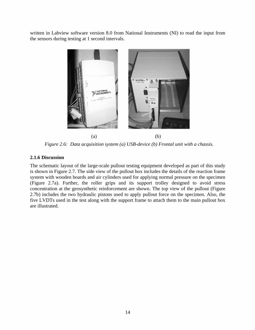
2.1.6 Discussion

The schematic layout of the large-scale pullout testing equipment developed as part of this study is shown in Figure 2.7. The side view of the pullout box includes the details of the reaction frame system with wooden boards and air cylinders used for applying normal pressure on the specimen (Figure 2.7a). Further, the roller grips and its support trolley designed to avoid stress concentration at the geosynthetic reinforcement are shown. The top view of the pullout (Figure 2.7b) includes the two hydraulic pistons used to apply pullout force on the specimen. Also, the five LVDTs used in the test along with the support frame to attach them to the main pullout box are illustrated.

15

Figure 2.7: Large scale pullout testing equipment: (a) Side view; (b) Top view.

The modified pullout box system with all the accessories is shown in Figure 2.8. The reaction frame system was found to be reliable means of applying uniform normal pressure on top of the geosynthetic specimen. Roller grips were found to be suitable means of clamping different kinds of geosynthetics used during the test. Further, the use of the new electric pump enabled better control over the rate of testing, as it could be independently controlled using the flow valve attached to it. Displacement transducers were attached to new system enabling faster data acquisition. The above changes led to reduction in test preparation time, better control over test procedure thereby providing repeatability among similar tests and reducing variability in test conditions for different geosynthetics. Overall, these modifications led to better equipment design capable of accurately characterizing low displacement soil-geosynthetic interface properties in the pullout box to be used for analysis using the proposed analytical model.

16

Figure 2.8: Large scale pullout box testing equipment

2.2 Large Pullout Testing Matrix

The experimental component of this study aimed at validating the analytical approach to analyze the pullout test results and determine the coefficient of soil-geosynthetic interaction (KSGI) (Chapter 4). Modifications were done to the original equipment used in the preliminary testing

17

phase to develop new equipment with capability of measuring low displacement soil-geosynthetic interaction.

The tests conducted on various geosynthetics along with test setup used for running a given pullout test are discussed. This is followed by explanation of the procedure followed to interpret results obtained from a given test to estimate the model parameters. The testing matrix incorporated four different geosynthetics (one geotextile and three geogrids). Two geogrids G1 (Tensar BX1100) and G2 (Mirafi BasXgrid11) were used along with a geotextile G3 (Mirafi Hp570) and another biaxial geogrid G4 (Tensar BX1200). Finally, the rationale for their selection and typical results for each one of them are described.

Based on the current literature, two major concerns are related to laboratory confined test procedures. First, it is difficult to establish repeatability of test results for a soil-geosynthetic system subjected to a given normal pressure. Second, the variability in test results reported in the literature is high enough where to distinguish between the performances of different geosynthetics. The present pullout testing scheme was planned to address these two issues. Therefore, preliminary set of tests were conducted on a geosynthetic to determine the capability of the present equipment to produce repeatable test results. Then the variability in the value of KSGI for a given test was established. After this initial calibration, various geosynthetics were tested to obtain the KSGI values under similar testing conditions and values obtained were compared. To incorporate these features, the overall large pullout testing scheme was grouped into three main series. Twenty large-scale pullout tests were conducted using four different kinds of geosynthetics as listed in Table 2.1. According to Palmeira (2008),

The geosynthetic reinforcements are generally modeled as linear elastic materials to match the model predictions. When simplifying assumptions are made, it is possible to make predictions fit reasonably well with the measurements for the geotextiles. However, in case of geogrids, if it is assumed as an equivalent rough planar reinforcement, predictions may deviate from measurements, depending on its geometrical characteristics and soil type.

Therefore while planning the pullout tests it was decided to conduct an initial series of tests using geotextile reinforcement. In the first series, eight tests were conducted. The baseline Test I-1 was conducted on geotextile specimen (G3) with sand as confining soil. The data analysis procedure adopted for interpreting results to compute model parameters (τy and Jc) and subsequently KSGI value for this test are explained in Chapter 4. The next Test I-2 was conducted to establish the repeatability of test results for the same soil-geosynthetic system as used in Test I-1. The results were analyzed to establish bounds on values of KSGI obtained from analysis of results for these two tests. The next three tests (I-3, I-4, and I-5) were conducted to quantify the effect of change in specimen dimensions (from that specified by ASTM standards) on the value of KSGI. In testes I-3 and I-4, the length of specimen was changed whereas the width was kept same as the initial specimen. In the Test I-5, the width of the specimen was decreased. These tests also helped in quantifying the effect of boundary conditions on the results. Then the effect of normal pressure on KSGI was evaluated by conducting a test at lower (I-6) and higher normal pressure (I-7) than used in Test I-1. Finally, the effect of specimen dimension was evaluated by running the test in machine direction (I-8) than cross-machine direction as used in the Test I-1. The first series of

18

tests helped in understanding various components that could influence KSGI value obtained from the pullout test for a given soil-geosynthetic system.

The second series of pullout tests consisted on eight tests conducted on two geogrid products (G1 and G4) manufactured with the same material. Based on the manufacturing process it was established that one product had slightly better performance properties than the other geogrid. The main objective of this phase of testing was to obtain KSGI values for both products and check if the predicted values reflected same performance order as expected based on their manufacturing quality. Three tests at normal pressures of 1, 3, and 5 psi (7, 21, and 35 kPa) were conducted on geogrid G1 (II-1, II-2, II-3) and geogrid G4 (II-4, II-5, II-6) similar to the baseline test (I-6, I-1 and I-7). Then two more tests, one for each geosynthetic were conducted in the machine direction (II-7 and II-8). The results obtained were used to compare the performance of products of known properties under pullout test conditions. Furthermore, these tests helped in verifying the applicability of the proposed model and parameter to pullout results on geogrid reinforcements.

In the third series, four tests were conducted on a geogrid (G2) obtained from different manufacturer. Tests III-1, III-2, and III-3 were conducted at normal pressures of 1, 3, and 5 psi (7, 21, and 35 kPa), respectively. The Test III-4 was conducted in different direction from the principal direction in Test III-2. The objective of this series of testing was to compare the performance of the geosynthetics manufactured using different material from those used in series II.

Overall, the aim of the pullout testing scheme was to establish evidence for capability of the proposed parameter to compare performance of various geosynthetics in the laboratory setting. The geosynthetics G1, G2, and G3 were also used in the field test sections. The performance predicted in terms of KSGI value from pullout test results for these geosynthetics was compared qualitatively with field measurements and is discussed in the Chapter 7.

19

Table 2.1: Testing matrix for large scale pullout testing

Series Test No.

Geosynthetic Type Direction

Normal pressure

Length Width Testing

rate Test characteristics

Comments

kPa (psi) m m mm/min

I

1 Geotextile G3 XD 21 (3) 0.60 0.45 1.0 Baseline

Test to calibrate the equipment and proposed

model

2 Geotextile G3 XD 21 (3) 0.60 0.45 1.0 Repeatability 3 Geotextile G3 XD 21 (3) 0.90 0.45 1.0 Effect of length 4 Geotextile G3 XD 21 (3) 0.30 0.45 1.0 Effect of length 5 Geotextile G3 XD 21 (3) 0.30 0.28 1.0 Effect of width 6 Geotextile G3 XD 7 (1) 0.60 0.45 1.0 Normal pressure 7 Geotextile G3 XD 35 (5) 0.60 0.45 1.0 Normal pressure 8 Geotextile G3 MD 21 (3) 0.60 0.45 1.0 Direction

II

1 Geogrid G1 XD 7 (1) 0.60 0.45 1.0 Normal pressure

Test conducted to compare performance of two geogrids from same

material.

2 Geogrid G1 XD 21 (3) 0.60 0.45 1.0 Normal pressure 3 Geogrid G1 XD 35 (5) 0.60 0.45 1.0 Normal pressure 4 Geogrid G4 XD 7 (1) 0.60 0.45 1.0 Normal pressure 5 Geogrid G4 XD 21 (3) 0.60 0.45 1.0 Normal pressure 6 Geogrid G4 XD 35 (5) 0.60 0.45 1.0 Normal pressure 7 Geogrid G1 MD 21 (3) 0.60 0.45 1.0 Direction8 Geogrid G4 MD 21 (3) 0.60 0.45 1.0 Direction

III

1 Geogrid G2 XD 7 (1) 0.60 0.45 1.0 Normal pressure Test conducted to predict the performance of

geosynthetics made of different material.

2 Geogrid G2 XD 21 (3) 0.60 0.45 1.0 Normal pressure 3 Geogrid G2 XD 35 (5) 0.60 0.45 1.0 Normal pressure 4 Geogrid G2 MD 21 (3) 0.60 0.45 1.0 Direction

Note: G1 – Geogrid Tensar BX1100; G2 – Geogrid Mirafi BasX11; G3 – Geotextile Mirafi HP570; G4 – Geogrid Tensar BX1200; XD – Cross Direction; MD – Machine Direction.

20

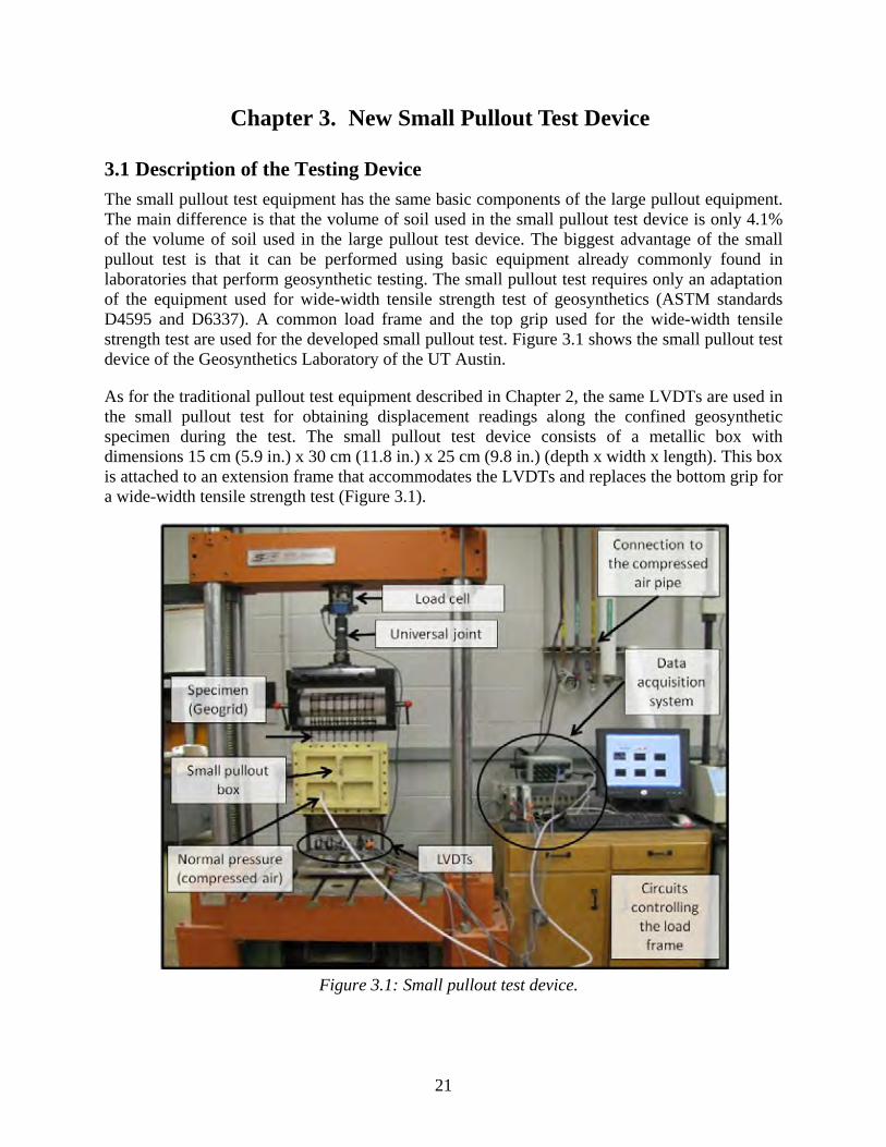
21

Chapter 3. New Small Pullout Test Device

3.1 Description of the Testing Device

The small pullout test equipment has the same basic components of the large pullout equipment. The main difference is that the volume of soil used in the small pullout test device is only 4.1% of the volume of soil used in the large pullout test device. The biggest advantage of the small pullout test is that it can be performed using basic equipment already commonly found in laboratories that perform geosynthetic testing. The small pullout test requires only an adaptation of the equipment used for wide-width tensile strength test of geosynthetics (ASTM standards D4595 and D6337). A common load frame and the top grip used for the wide-width tensile strength test are used for the developed small pullout test. Figure 3.1 shows the small pullout test device of the Geosynthetics Laboratory of the UT Austin.

As for the traditional pullout test equipment described in Chapter 2, the same LVDTs are used in the small pullout test for obtaining displacement readings along the confined geosynthetic specimen during the test. The small pullout test device consists of a metallic box with dimensions 15 cm (5.9 in.) x 30 cm (11.8 in.) x 25 cm (9.8 in.) (depth x width x length). This box is attached to an extension frame that accommodates the LVDTs and replaces the bottom grip for a wide-width tensile strength test (Figure 3.1).

Figure 3.1: Small pullout test device.

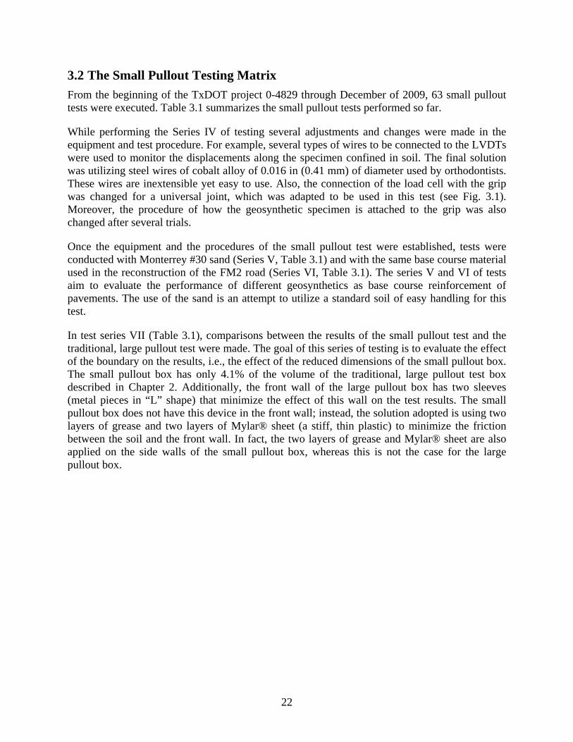
22

3.2 The Small Pullout Testing Matrix

From the beginning of the TxDOT project 0-4829 through December of 2009, 63 small pullout tests were executed. Table 3.1 summarizes the small pullout tests performed so far.

While performing the Series IV of testing several adjustments and changes were made in the equipment and test procedure. For example, several types of wires to be connected to the LVDTs were used to monitor the displacements along the specimen confined in soil. The final solution was utilizing steel wires of cobalt alloy of 0.016 in (0.41 mm) of diameter used by orthodontists. These wires are inextensible yet easy to use. Also, the connection of the load cell with the grip was changed for a universal joint, which was adapted to be used in this test (see Fig. 3.1). Moreover, the procedure of how the geosynthetic specimen is attached to the grip was also changed after several trials.

Once the equipment and the procedures of the small pullout test were established, tests were conducted with Monterrey #30 sand (Series V, Table 3.1) and with the same base course material used in the reconstruction of the FM2 road (Series VI, Table 3.1). The series V and VI of tests aim to evaluate the performance of different geosynthetics as base course reinforcement of pavements. The use of the sand is an attempt to utilize a standard soil of easy handling for this test.

In test series VII (Table 3.1), comparisons between the results of the small pullout test and the traditional, large pullout test were made. The goal of this series of testing is to evaluate the effect of the boundary on the results, i.e., the effect of the reduced dimensions of the small pullout box. The small pullout box has only 4.1% of the volume of the traditional, large pullout test box described in Chapter 2. Additionally, the front wall of the large pullout box has two sleeves (metal pieces in “L” shape) that minimize the effect of this wall on the test results. The small pullout box does not have this device in the front wall; instead, the solution adopted is using two layers of grease and two layers of Mylar® sheet (a stiff, thin plastic) to minimize the friction between the soil and the front wall. In fact, the two layers of grease and Mylar® sheet are also applied on the side walls of the small pullout box, whereas this is not the case for the large pullout box.

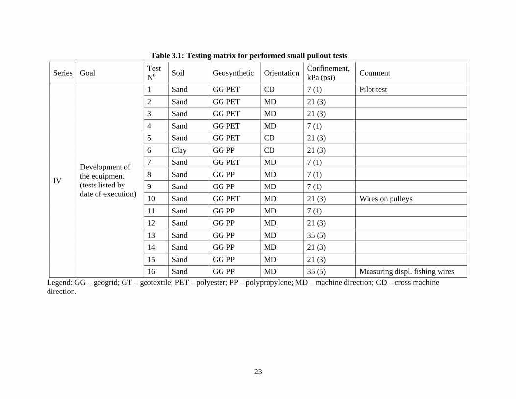
23

Table 3.1: Testing matrix for performed small pullout tests

Series Goal Test No

Soil Geosynthetic Orientation Confinement, kPa (psi)

Comment

IV

Development of the equipment (tests listed by date of execution)

1 Sand GG PET CD 7 (1) Pilot test

2 Sand GG PET MD 21 (3)

3 Sand GG PET MD 21 (3)

4 Sand GG PET MD 7 (1)

5 Sand GG PET CD 21 (3)

6 Clay GG PP CD 21 (3)

7 Sand GG PET MD 7 (1)

8 Sand GG PP MD 7 (1)

9 Sand GG PP MD 7 (1)

10 Sand GG PET MD 21 (3) Wires on pulleys

11 Sand GG PP MD 7 (1)

12 Sand GG PP MD 21 (3)

13 Sand GG PP MD 35 (5)

14 Sand GG PP MD 21 (3)

15 Sand GG PP MD 21 (3)

16 Sand GG PP MD 35 (5) Measuring displ. fishing wires Legend: GG – geogrid; GT – geotextile; PET – polyester; PP – polypropylene; MD – machine direction; CD – cross machine direction.

24

Table 3.1: Testing matrix for performed small pullout tests (cont.)

Series Goal Test No

Soil Geosynthetic Orientation Confinement,kPa (psi)

Comment

IV

Development of the equipment (tests listed by date of execution)

17 Clay GG PP CD 21 (3)

18 Sand GG PP CD 7 (1)

19 Sand GG PP CD 21 (3) Measuring displacement with orthodontic steel wires

20 Sand GG PET CD 21 (3)

21 Sand GT MD 21 (3)

22 Sand GT MD 35 (5)

23 Sand GT MD 21 (3)

24 Sand GT MD 7 (1)

25 Sand GT MD 35 (5)

26 Sand GT MD 21 (3)

27 Sand GT CD 21 (3)

28 Sand GT MD 21 (3)

29 Sand GT MD 21 (3)

V

Comparison of the performance of the geosynthetics confined in sand

1 Sand GG PP MD 21 (3)

2 Sand GG PP CD 21 (3)

3 Sand GG PP CD 35 (5)

4 Sand GG PET MD 21 (3)

5 Sand GG PET MD 21 (3) Legend: GG – geogrid; GT – geotextile; PET – polyester; PP – polypropylene; MD – machine direction; CD – cross machine direction.

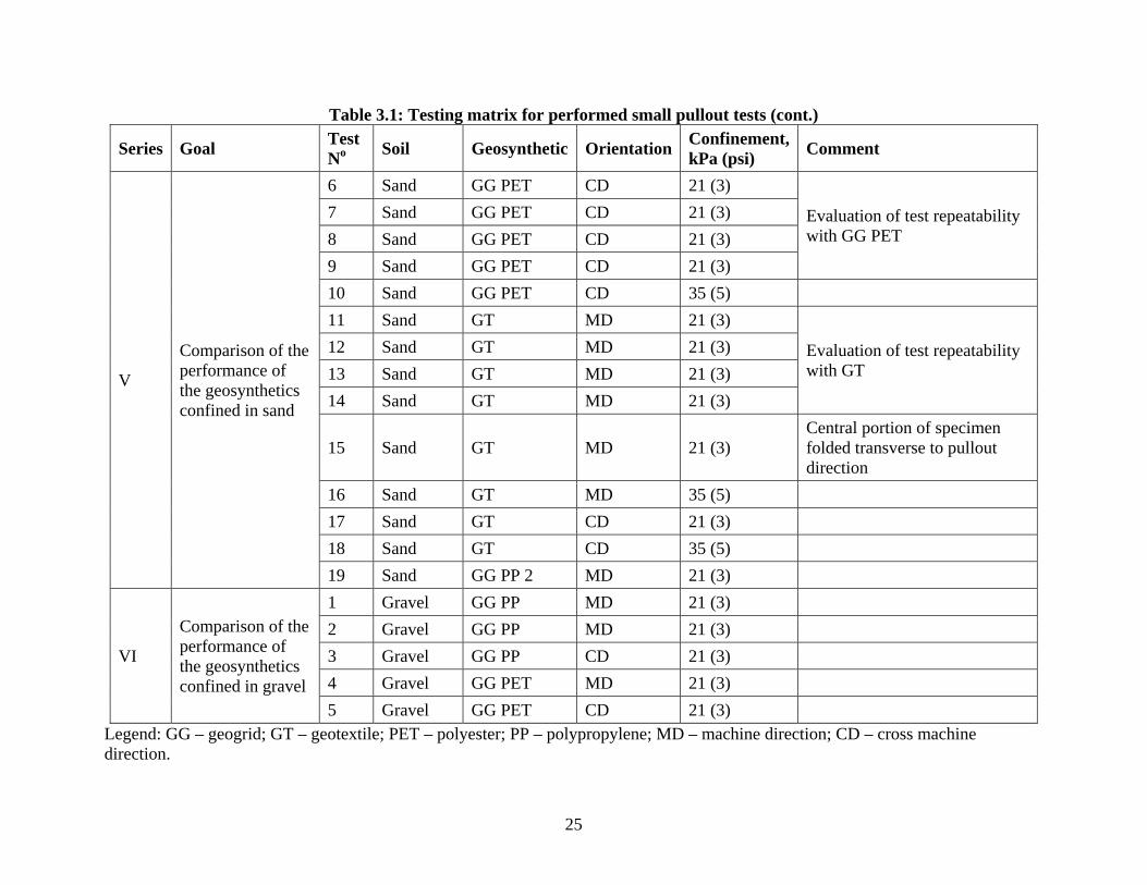
25

Table 3.1: Testing matrix for performed small pullout tests (cont.)

Series Goal Test No

Soil Geosynthetic Orientation Confinement,kPa (psi)

Comment

V

Comparison of the performance of the geosynthetics confined in sand

6 Sand GG PET CD 21 (3)

Evaluation of test repeatability with GG PET

7 Sand GG PET CD 21 (3)

8 Sand GG PET CD 21 (3)

9 Sand GG PET CD 21 (3)

10 Sand GG PET CD 35 (5)

11 Sand GT MD 21 (3)

Evaluation of test repeatability with GT

12 Sand GT MD 21 (3)

13 Sand GT MD 21 (3)

14 Sand GT MD 21 (3)

15 Sand GT MD 21 (3) Central portion of specimen folded transverse to pullout direction

16 Sand GT MD 35 (5)

17 Sand GT CD 21 (3)

18 Sand GT CD 35 (5)

19 Sand GG PP 2 MD 21 (3)

VI

Comparison of the performance of the geosynthetics confined in gravel

1 Gravel GG PP MD 21 (3)

2 Gravel GG PP MD 21 (3)

3 Gravel GG PP CD 21 (3)

4 Gravel GG PET MD 21 (3)

5 Gravel GG PET CD 21 (3) Legend: GG – geogrid; GT – geotextile; PET – polyester; PP – polypropylene; MD – machine direction; CD – cross machine direction.

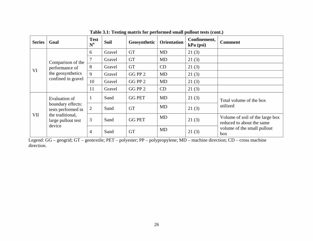
26

Table 3.1: Testing matrix for performed small pullout tests (cont.)

Series Goal Test No

Soil Geosynthetic Orientation Confinement,kPa (psi)

Comment

VI

Comparison of the performance of the geosynthetics confined in gravel

6 Gravel GT MD 21 (3)

7 Gravel GT MD 21 (3)

8 Gravel GT CD 21 (3)

9 Gravel GG PP 2 MD 21 (3)

10 Gravel GG PP 2 MD 21 (3)

11 Gravel GG PP 2 CD 21 (3)

VII

Evaluation of boundary effects: tests performed in the traditional, large pullout test device

1 Sand GG PET MD 21 (3) Total volume of the box utilized 2 Sand GT MD 21 (3)

3 Sand GG PET MD 21 (3) Volume of soil of the large box reduced to about the same volume of the small pullout box 4 Sand GT MD 21 (3)

Legend: GG – geogrid; GT – geotextile; PET – polyester; PP – polypropylene; MD – machine direction; CD – cross machine direction.

27

Chapter 4. The KSGI Model for Analysis of Pullout Test Data under Low Displacements

Various theoretical and empirical procedures have been developed in order to model the soil-geosynthetic interface mechanism during pullout. These procedures can be grouped into two broad categories: limit equilibrium method and analytical methods. The limit equilibrium methods neither give sufficient information on the pullout force nor displacement and strains developed in the reinforcements prior to failure (Rowe and Mylleville, 1994). On the other hand, analytical methods can be used to predict displacement, strains, and force generated in the reinforcement during the deformation as well as failure (Sugimoto and Alagiyawanna 2003).

Analytical solutions to interpret and analyze data obtained by pullout test have been proposed by Juran and Chen (1988), Yuan and Chua (1991), Abramento and Whittle (1995), Sobhi and Wu (1996), Alobaidi et al. (1997), Madhav et al. (1998), Perkins and Cuelho (1999), Palmeira (2004), and Teixeira et al. (2007). These models vary in their assumptions with respect to the constitutive material properties, the load transfer mechanism at the interface, and the shape of the load-strain curve during pullout. In general, these analytical models are used to predict the load-displacement curve of soil-geosynthetic system under confinement.

The analytical models for pullout test interpretation were developed for MSE wall design and focus on predicting the maximum pullout force magnitudes. Because the focus of current analytical solutions is prediction of failure conditions, the displacement profile from frontal LVDT is the only displacement value used to predict the response of the geosynthetic for given load magnitude. However, the primary goal of pullout tests in the present implementation project is the initial stiffness of the soil geosynthetic interface and it required a model that could capture small displacement behavior for application to reinforced pavement design.

This section describes the differential equation governing the behavior of soil-geosynthetic interaction in the pullout test. Then, the methods proposed by current analytical models to solve this equation are listed. Finally, the limitations of these solutions for their applicability to reinforced pavement design are discussed.

4.1 Governing Differential Equation

A pullout test is conducted by sandwiching a geosynthetic of known length, L, and width, W, between two soil layers inside the pullout box. Normal pressure is then applied on the top of the soil-geosynthetic interface to represent the field conditions under which geosynthetic is expected to perform. Finally, the geosynthetic is clamped at the loading grips and is pulled out of the box assembly at a constant rate of displacement and the required force is measured. The pullout force F measured during the pullout test is generally reported as a normalized value per unit width of the specimen and has units of force per unit width (i.e., lb/ft or kN/m). The same convention was used throughout this analysis.

Geosynthetics are categorized as extensible and inextensible reinforcements depending on strain magnitude required in mobilizing the maximum tensile strength. For inextensible geosynthetics the peak strain values range between 2%-5% whereas for extensible geosynthetics they are greater than 10%. McGown et al. (1978) reported different load-deformation response for soil

28

reinforced with these reinforcements as shown in Figure 4.1. In this study, the soil-geosynthetics interaction behavior was analyzed in small displacements regime.

Figure 4.1: Axial load-strain relationship for soil reinforced with various reinforcements

(adapted from McGown et al., 1978).

4.2 Shear Stress-Confined Force Relationship

Consider a geosynthetic element of length ∂x, confined inside the pullout box and subjected to force F in the pullout direction. Then the shear stress τ(x) is mobilized along its surface, such that the force is dissipated along its length. Assuming no extensibility of reinforcement, the free body diagram for points A and B on the either side of the element can be given as shown in Figure 4.2.

Figure 4.2: Free body diagram for geosynthetic element of length ∂x in pullout test.

The force equilibrium can then be written in differential form as follows:

dxxxdFxFxF ).(.2))()(()( τ=−− (4.1)

dx

xdFx

)(.

2

1)( =τ (4.2)

Let us assume that strain ε(x) develops in the element of length dx due to the change in confined force (dF) between two points. Then, the confined force and strain are related through confined stiffness Jc of the geosynthetic and is given as,

F F-dF

τ.dx

τ.dx

A B

29

)(.)( xJxF c ε= (4.3)

The strain developed in the geosynthetic element of length dx can then be related to the displacement in the reinforcement, dwr, as:

x

xwx r

∂∂

=)(

)(ε (4.4)

By substituting Equation 4.4 into Equation 4.3,

x

xwJxF r

c ∂∂= )(

.)( (4.5)

Differentiating above equation with respect to x, gives

2

2 )(.

)(

x

xwJ

x

xF rc ∂

∂=

∂∂

(4.6) Substituting Equation 4.6 into Equation 4.1 gives,

2

2 )(.

2

1)(

x

xwJx r

c ∂∂

=τ (4.7)

c

r

J

x

x

xw )(.2)(2

2 τ=∂

∂

(4.8) The above expression is a second-order differential equation governing the soil-geosynthetic interface behavior during the pullout test. The equation relates the displacement wr(x) with the shear stress τ(x) developed at the soil-geosynthetic interface in terms of confined stiffness Jc, for geosynthetic element of length ∂x in the pullout test.

4.3 Assumptions Involved

The expression derived in Section 4.2 was used to predict the behavior of the soil-geosynthetic interface in a pullout test is a second-order differential equation. The solution to the governing equation requires defining three relationships. The first relation defines shape of force-strain curve for the given geosynthetic element for computing the value of confined stiffness Jc. The second relation defines the value of the relative displacement wr of the reinforcement in relation to the soil. Finally, the distribution of shear stress τ(x) for given displacement wr (x) for an element of length dx, needs to be defined. Perkins and Cuelho (1999) developed the solution for

30

the governing equation of geosynthetic element in a pullout test using assumptions related to each of the above relationships. The three assumptions were related to:

• Geosynthetic load-strain relationship

• Absolute movement of soil surrounding the geosynthetic

• Relationship to describe shear stress-displacement response Based on the assumptions made, the governing equation can then be solved by incorporating appropriate boundary condition for a given pullout force measured during the test, to obtain the distribution of displacement along the length of the geosynthetic and quantify the soil-geosynthetic interface.

4.3.1 Geosynthetic Load-Strain Relationship

An assumption is required for predicting the confined stiffness of the geosynthetic during the pullout test. It has been modeled as linear (Wilson-Fahmy et al., 1994), non-linear (Perkins and Cuelho, 1999), or equal to unconfined stiffness of the geosynthetic obtained from the wide-width in air tensile test (Ochiai et al. 1996, Sierra et al. 2009).

In the solution proposed in this study, the force-strain relationship for a given geosynthetic was assumed linear and proportional to the confined stiffness of the soil-geosynthetic system. It differs from the current models that assume a linear relation based on the stiffness of the geosynthetic obtained from the unconfined tensile test to predict the behavior under confinement. Due to interlocking in geogrids or impregnation of geotextiles with the surrounding soil, the transverse ribs or fibers are mobilized, leading to additional components that help dissipate the load throughout the length of the geosynthetic. This is not captured by the stiffness value of the geosynthetic obtained from isolated unconfined tensile tests in uniaxial direction. This assumption better represents the response of geosynthetics under pullout test conditions as shown in Figure 4.3. Therefore, under confinement, geogrids mobilize the junctions of longitudinal and transverse ribs that do not occur under unconfined loading conditions.

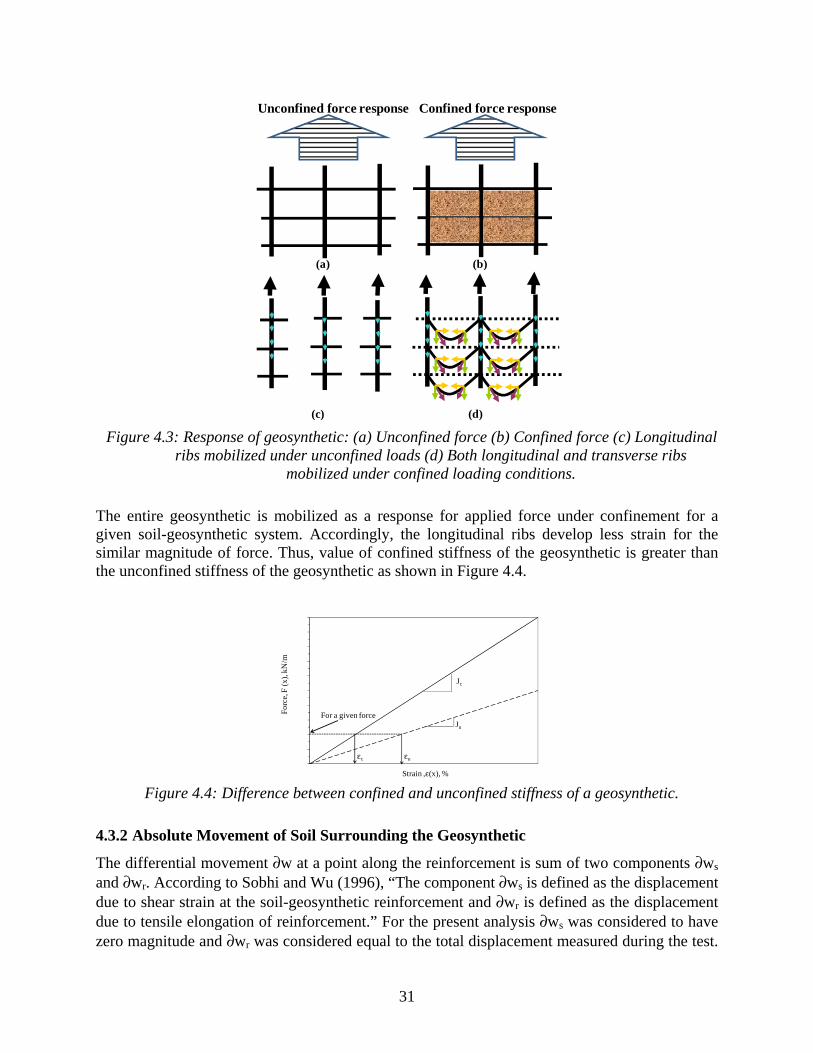
31

Figure 4.3: Response of geosynthetic: (a) Unconfined force (b) Confined force (c) Longitudinal

ribs mobilized under unconfined loads (d) Both longitudinal and transverse ribs mobilized under confined loading conditions.

The entire geosynthetic is mobilized as a response for applied force under confinement for a given soil-geosynthetic system. Accordingly, the longitudinal ribs develop less strain for the similar magnitude of force. Thus, value of confined stiffness of the geosynthetic is greater than the unconfined stiffness of the geosynthetic as shown in Figure 4.4.

Figure 4.4: Difference between confined and unconfined stiffness of a geosynthetic.

4.3.2 Absolute Movement of Soil Surrounding the Geosynthetic

The differential movement ∂w at a point along the reinforcement is sum of two components ∂ws and ∂wr. According to Sobhi and Wu (1996), “The component ∂ws is defined as the displacement due to shear strain at the soil-geosynthetic reinforcement and ∂wr is defined as the displacement due to tensile elongation of reinforcement.” For the present analysis ∂ws was considered to have zero magnitude and ∂wr was considered equal to the total displacement measured during the test.

Unconfined force response

(a) (b)

(c) (d)

Confined force response

0

10

20

30

40

50

60

70

80

90

100

For

ce, F

(x)

, kN

/m

Strain ,ε(x), %

Jc

Ju

For a given force

εc εu

32

In other words, the soil is assumed stationary and all the displacement measured during the test is assumed to occur in the geosynthetic reinforcement, which equals the displacement at the interface. Sobhi and Wu (1996) assumed no slippage occurs at the soil-reinforcement interface and the displacement undergone by the soil and reinforcement in a bonded manner is negligible. The above assumption can be expressed in the mathematical form using the following equations:

)()()( xwxwxw rs ∂+∂=∂ (4.9)

0)( =∂ xws (4.10) )()( xwxw r∂=∂ (4.11)

4.3.3 Shear Stress- Relative Displacement Relationship at the Interface

Juran and Chen (1988) indicate that modeling of the load transfer mechanism generated in a pullout test requires an appropriate interaction law to relate the shear stress mobilized at any point of the interface to the reinforcement displacement. In previous studies, the distribution of shear stress has been assumed constant (Sobhi and Wu, 1996), linear (Abdelouhab et al., 2008), bi-linear (Juran and Chen 1988, Madhav et al. 1999), non-linear (Perkins and Cuelho, 1999) or hyperbolic (Gurung and Iwao, 1998) with increasing geosynthetic displacement magnitude. Also, Sugimoto and Alagiyawanna (2003) showed that the direct evaluation of the interface properties from the ultimate state may not be appropriate to simulate the actual geosynthetic behavior in reinforced soil masses before failure in a pullout test. Sobhi and Wu (1996) defined a limit shear stress for a pullout test that was lower than the maximum shear stress and a function of overburden pressure applied to the soil-geosynthetic interface. They showed results from finite element analyses indicating development of uniform shear stress independent of the frontal pullout force magnitude and length of the geosynthetic.

The analyses in this study assumes a parameter called as yield shear stress (τy), which is assumed to be uniform over the active length of the reinforcement (explained in Section 4.2). The yield shear stress is a key parameter for a given soil-geosynthetic system subjected to normal pressure and is independent of the displacement at a point along the confined length of geosynthetic as shown in Figure 4.5. It is computed based on the movement of LVDTs used in the test and has lower magnitude than that obtained from maximum pullout conditions (τmax). In principal, the yield shear stress is a parameter that accounts for shear, bearing, and passive mechanisms experienced by the geosynthetic in the pullout box at small displacements.

The above assumptions can be used to solve the governing differential equation for the pullout test of a geosynthetic. The solution can be used to obtain the displacement, strain and force at any point x along the length of the geosynthetic. Derivation of the governing differential equation is discussed in this chapter.

33

Figure 4.5: Shear stress distribution as a function of displacement at a given point

4.4 Displacement Distribution along Geosynthetic Length

Assuming that the shear stress is constant and equal to the yield shear stress τy, and substituting ∂w for ∂wr as derived in Equation 4.11, the governing differential Equation 4.8 at any given time t for a given frontal pullout force, can be written as,

c

y

Jx

xw τ.2)(2

2

=∂

∂

(4.12)

Two model parameters are τy and Jc. Previously, both parameters were assumed to have a unique value for a given pullout test. Therefore, the right hand side of Equation 4.12 can be assumed constant and be replaced by β:

βτ

=c

y

J

.2

(4.13) where β is a constant. Substituting Equation 4.13 into Equation 4.12,

β=∂

∂2

2 )(

x

xw (4.14)

Integrating both sides, we obtain

1.)(

Cxx

xw +=∂

∂ β (4.15)

0

1

2

3

4

5

6

0 1 2 3 4 5 6 7 8 9 10 11 12 13 14 15

She

ar s

tres

s, τ y

, kN

/m2

Displacement (mm)

τy

34

Then the strain at any confined point x can be expressed as shown in Equation 4.15 and can be written as:

1.)( Cxx += βε (4.16) Then the force at any point x can be given by substituting the Equation 4.16 in Equation 4.13,

)..()(.)( 1CxJxJxF cc +== βε (4.17)

Further integrating both sides of Equation 4.15, leads to

212 ..

2

1)( CxCxxw ++= β

(4.18) where C1 and C2 are constants whose values can be estimated using boundary conditions. The expressions derived in Equations 4.16, 4.17 and 4.18 above can be used to predict the strain, force and displacement profile at any point x within the pullout box in terms of model parameters τy and Jc provided C1 and C2 are known.

4.5 Boundary Conditions

The governing differential equation for the pullout test is of the second-order form and requires values of two coefficients for complete solution. These coefficients are required to obtain the distribution of the displacement profile for a given force along the length of the geosynthetic as shown in Equation 4.18. The coefficient values are computed based on the boundary conditions adopted by a given model while proposing a solution to the governing equation. The boundary conditions involve knowing two quantities at a given instant of time. These are generally force at pullout end and displacement at other end of the specimen. Therefore, a known force value at one boundary and known displacement value at other boundary at any given instant of time can be used to solve for both coefficients.

For the force boundary condition, the force at pullout end of the specimen is known at any given time and can be used to solve for one coefficient (C1 in this case). Because the analytical solutions for pullout test were developed in previous studies to assess the collapse of MSE walls, the focus has to be modeling of the failure conditions. Therefore, the displacement boundary condition in these solutions was based on the mobilization of the entire length of the geosynthetic. It was assumed that when maximum pullout force was reached in a given test, the entire length of the geosynthetic is mobilized and displacement at the embedded end is zero. This condition was then used to solve for second coefficient (C2 in this case). The magnitudes of these coefficients were finally used for predicting the displacement distribution for the entire geosynthetic length at failure.

35

However, the applicability of pullout tests to reinforced pavement design involves understanding of the soil-geosynthetic interface stiffness developed at low displacement magnitudes. The solution is thus required to model the entire frontal force and displacement curve for a pullout test with emphasis on capturing the initial displacement mobilized at the interface. In other words, the solution requires a displacement boundary condition such that it can be solved for increment of frontal pullout force value throughout the test and not the maximum pullout force alone. The displacement values for a given frontal force can be obtained by integrating the strain profile over the entire length of the geosynthetic. Consequently, solutions for second coefficient have involved assuming a strain distribution and solving it to predict the subsequent displacement profile for the entire geosynthetic length.

Two methods have been proposed in the literature to solve the coefficient for second boundary condition in regards with strain distribution. The first approach involves solving the displacement boundary by assuming constant strain distribution over the entire length of the geosynthetic. The second approach involves assuming a linear distribution of strain and substituting the value for the coefficient from another test like wide width tensile test or direct shear test. This solution is then used to predict displacement profile along the length of the geosynthetic. Thus, these models proposed in the literature utilize the force boundary condition at the pullout end and assume one of the possibilities listed above to substitute for the second boundary condition. The limitations of these methods to solve for displacement boundary condition are discussed in Sections 4.5.1 and 4.5.2.

4.5.1 Constant Strain Distribution A constant strain distribution assumes the uniform strain between two measurement points. Then the average strain between these points is calculated based on the displacement measurements made using LVDTs during the test. This approach was proposed by Ochiai et al., (1996) and the strain throughout the entire length of the geosynthetic was assumed as a step function.

The above assumption is illustrated in Figure 4.6. Consider a geosynthetic of confined length L subjected to pullout force Fp at a given time t, as shown in Figure 4.6a. Then let x1, x2 and x3 be three points on the geosynthetic such that the distance between 1 and 2 is L1 and 2 and 3 is L2. Also, the displacements for given force are d1, d2 and d3 at these three points. Then using the above assumption of constant strain, its value can be calculated. The resulting strain and displacement profile predicted based on above assumption is shown in Figure 4.6b and 4.6c respectively.

Based on model assumptions it can be seen that strain is a linear function whereas displacement is a quadratic function over the length of the geosynthetic for given frontal pullout force (as shown in Equation 4.16 and 4.18). However, the assumption of constant strain leads to linear distribution of displacement along the length of the geosynthetic—i.e., the value for the second coefficient is assumed zero. The equation for displacement distribution can be obtained for the given geosynthetic under pullout conditions by integration of the strain relationship. The actual strain profile is not a series of discrete values but a continuous function along the entire length of the geosynthetic whose magnitude decreases from pullout end to the embedded end.

36

This approach under predicts the strain magnitude at points closer to the pullout end and over predicts the strain at point closer to the embedded end of the geosynthetic. Furthermore, based on pullout test results conducted as part of this implementation project it was observed that the actual displacement profile along the length of the geosynthetic is parabolic in shape rather than linear. Therefore, the constant strain assumption leads to error in displacement prediction at low strain magnitudes.

Figure 4.6: Predictions based on constant strain distribution: (a) Schematic of displacement

profile for given pullout force (b) actual vs. predicted strain distribution (c) actual vs. predicted displacement.

4.5.2 Linear Strain Distribution This assumption involves modeling the strain distribution as a continuous function over the mobilized length of the geosynthetic. The solutions incorporating boundary condition based on this hypothesis represent the model conditions realistically. Two approaches have been reported in the literature to model this behavior.

The first approach involves assuming the strain distribution under confined conditions in the reinforcement equals that under unconfined conditions. In other words, these models assume confined stiffness equal to the unconfined stiffness of the geosynthetic. Then knowing the frontal force, the strain magnitude is calculated as shown in Equation 4.17. Once the strain magnitude is known, the displacement value can be calculated by integrating Equation 4.16. Sierra et al. (2009) proposed a load transfer model to predict force-displacement relationship of the geogrid

Pullout force end

Confined length end

L1 L2

d1d2 d3

εx

dx

x

x

x1 x2 x3

x1 x2 x3

x1 x2 x3

Actual

Predicted

Actual

Predicted

FP, at any time t

1

2112 L

dd −=ε

2

3223 L

dd −=ε

(a)

(b)

(c)

37

under pullout conditions by subdividing it into rheological units but used load–elongation curves from tensile tests on the geogrids. The other approach involves developing the entire solution and then calibrating the second coefficient from a test other than the pullout test. Sobhi and Wu (1996) proposed a model to predict pullout force and displacement at a point under confined conditions but it required another test as proposed by Ling et al. (1992) to calibrate the model. The drawback of this approach is that the strain levels used to calibrate the parameter are different from one observed in the pullout test. This leads to test results that are sensitive to small changes in value of the assumed parameter. Furthermore, this approach does not utilize all the displacement data obtained using various LVDTs across the length of the geosynthetic but uses only frontal LVDT to match the results.

4.6 Discussion

The current analytical solutions either incorporate the limited data obtained from the pullout test or use other tests to predict the model parameters. The assumptions made in the current models with regard to second boundary condition lead to errors that are critical when predicting the behavior of the soil-geosynthetic interface at regime of low displacements. However, the primary goal of pullout tests in the present implementation project was the application to reinforced pavement design. To avoid any unrealistic assumptions, the proposed model in this implementation project suggests a new approach to compute the second boundary condition. The data obtained from LVDTs at various points along the length of the geosynthetic is taken into account to model the soil-geosynthetic behavior realistically.

4.7 Soil-Geosynthetic Interaction Model

The solution for governing differential equation of the pullout test involves two coefficients. The first coefficient can be computed by using the force boundary condition at the pullout end of the geosynthetic. The second coefficient is computed using assumption regarding strain distribution within the geosynthetic for a given force level. The limitations of this approach were discussed in the section 4.6. The soil-geosynthetic interaction (SGI) model is proposed as part of this implementation project that involves a different approach in terms of displacement rather than strain values to compute the second boundary condition for the pullout test.

Specifically, rather than assuming the strain distribution for a given geosynthetic, the incremental distance travelled by increase in frontal pullout force through the confined geosynthetic specimen length during the test is monitored. In other words, the length of geosynthetic mobilized for a given frontal pullout force value is computed. This concept was proposed by Sobhi and Wu (1996) and called active length of reinforcement where the force is zero within the embedded geosynthetic for a given magnitude of frontal pullout force. The similar definition for active length (L’) of the geosynthetic was adopted in the present model. However, it is different from the total length (L) of geosynthetic specimen used in the pullout test, which is a fixed quantity and does not vary with frontal pullout force during the test. The active length increases with increasing frontal pullout force and becomes equal to the total length only when the entire geosynthetic is mobilized.

The SGI model uses this concept of active length to define the second boundary condition during the pullout test. The active length of the geosynthetic for a given frontal pullout force value is the

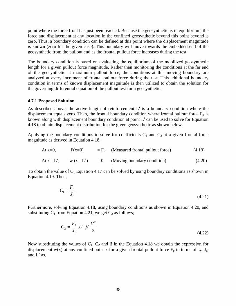
38

point where the force front has just been reached. Because the geosynthetic is in equilibrium, the force and displacement at any location in the confined geosynthetic beyond this point beyond is zero. Thus, a boundary condition can be defined at this point where the displacement magnitude is known (zero for the given case). This boundary will move towards the embedded end of the geosynthetic from the pullout end as the frontal pullout force increases during the test.

The boundary condition is based on evaluating the equilibrium of the mobilized geosynthetic length for a given pullout force magnitude. Rather than monitoring the conditions at the far end of the geosynthetic at maximum pullout force, the conditions at this moving boundary are analyzed at every increment of frontal pullout force during the test. This additional boundary condition in terms of known displacement magnitude is then utilized to obtain the solution for the governing differential equation of the pullout test for a geosynthetic.

4.7.1 Proposed Solution

As described above, the active length of reinforcement Lʹ is a boundary condition where the displacement equals zero. Then, the frontal boundary condition where frontal pullout force Fp is known along with displacement boundary condition at point Lʹ can be used to solve for Equation 4.18 to obtain displacement distribution for the given geosynthetic as shown below.

Applying the boundary conditions to solve for coefficients C1 and C2 at a given frontal force magnitude as derived in Equation 4.18,

At x=0, F(x=0) = FP (Measured frontal pullout force) (4.19)

At x=-L’, w (x=-L’) = 0 (Moving boundary condition) (4.20) To obtain the value of C1 Equation 4.17 can be solved by using boundary conditions as shown in Equation 4.19. Then,

c

P

J

FC =1

(4.21) Furthermore, solving Equation 4.18, using boundary conditions as shown in Equation 4.20, and substituting C1 from Equation 4.21, we get C2 as follows;

2

'.'.

2

2

LL

J

FC

c

P β−= (4.22)

Now substituting the values of C1, C2 and β in the Equation 4.18 we obtain the expression for displacement w(x) at any confined point x for a given frontal pullout force Fp in terms of τy, Jc, and L’ as,

39

22 '.'...)( LJ

LJ

Fx

J

Fx

Jxw

c

y

c

P

c

P

c

y ττ−++=

(4.23) Rearranging,

)]'([)'(

)( xLFJ

xLxw yP

C

−−+= τ (4.24)

To obtain the strain distribution, the above equation can be differentiated with respect to x, the strain ε(x) at any point can be given as,

].2[1)(

)( xFJx

xwx yP

C

τε +=∂

∂= (4.25)

Then the force at any point x can be given by substituting the expression above in Equation 4.17,

xFxJxF yPc τε .2)(.)( +== (4.26)

Furthermore, for a given pullout force Fp, the force at point L’ (i.e., at the end of the boundary) is zero. Thus, substituting for x = -L’ in Equation 4.26, we obtain

0'..2)'( =−=−= LFLxF yP τ (4.27)

y

PFL

τ.2'=

(4.28) Thus, the point L’ where the force front has just been reached for a given frontal pullout force can be calculated knowing the yield shear stress parameter. Substituting the above expression for L’ in Equation 4.24, the displacement distribution can be obtained in terms of model parameters τy and Jc as,

cy

P

c

P

c

y

J

Fx

J

Fx

Jxw

..4..)(

22

ττ

++= (4.29)

Thus, using the Equations 4.24, 4.25 and 4.29, strain ε(x), force F(x) and the displacement w(x) at a point x can be calculated for a given frontal pullout force Fp in terms of yield shear stress, τy and confined stiffness Jc of the geosynthetic.

4.7.2 Parameter for Geosynthetic Reinforced Pavement

The boundary conditions used to solve the governing differential equation for the pullout test was explained in Section 4.7.1. However, the focus of conducting the pullout tests was to

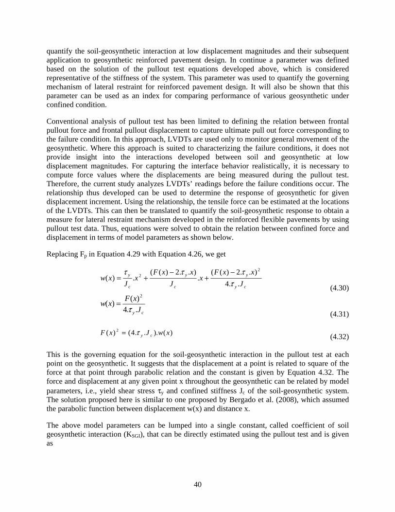
40

quantify the soil-geosynthetic interaction at low displacement magnitudes and their subsequent application to geosynthetic reinforced pavement design. In continue a parameter was defined based on the solution of the pullout test equations developed above, which is considered representative of the stiffness of the system. This parameter was used to quantify the governing mechanism of lateral restraint for reinforced pavement design. It will also be shown that this parameter can be used as an index for comparing performance of various geosynthetic under confined condition.

Conventional analysis of pullout test has been limited to defining the relation between frontal pullout force and frontal pullout displacement to capture ultimate pull out force corresponding to the failure condition. In this approach, LVDTs are used only to monitor general movement of the geosynthetic. Where this approach is suited to characterizing the failure conditions, it does not provide insight into the interactions developed between soil and geosynthetic at low displacement magnitudes. For capturing the interface behavior realistically, it is necessary to compute force values where the displacements are being measured during the pullout test. Therefore, the current study analyzes LVDTs’ readings before the failure conditions occur. The relationship thus developed can be used to determine the response of geosynthetic for given displacement increment. Using the relationship, the tensile force can be estimated at the locations of the LVDTs. This can then be translated to quantify the soil-geosynthetic response to obtain a measure for lateral restraint mechanism developed in the reinforced flexible pavements by using pullout test data. Thus, equations were solved to obtain the relation between confined force and displacement in terms of model parameters as shown below.

Replacing Fp in Equation 4.29 with Equation 4.26, we get

cy

y

c

y

c

y

J

xxFx

J

xxFx

Jxw

..4

)..2)((.

)..2)((.)(

22

ττττ −

+−

+= (4.30)

cy J

xFxw

..4

)()(

2

τ=

(4.31)

)()...4()( 2 xwJxF cyτ= (4.32) This is the governing equation for the soil-geosynthetic interaction in the pullout test at each point on the geosynthetic. It suggests that the displacement at a point is related to square of the force at that point through parabolic relation and the constant is given by Equation 4.32. The force and displacement at any given point x throughout the geosynthetic can be related by model parameters, i.e., yield shear stress τy and confined stiffness Jc of the soil-geosynthetic system. The solution proposed here is similar to one proposed by Bergado et al. (2008), which assumed the parabolic function between displacement w(x) and distance x.

The above model parameters can be lumped into a single constant, called coefficient of soil geosynthetic interaction (KSGI), that can be directly estimated using the pullout test and is given as

41

cySGI JK ..4τ= (4.33)

Then Equation 4.32 can be written as

)(.)( 2 xwKxF SGI= (4.34) According to Bonaparte et al. (1987), “There are two important soil-reinforcement interaction characteristics for design: soil reinforcement interface shear behavior and the influence of soil confinement on tensile characteristics of the reinforcement.” Therefore, constant KSGI allows for combing both these characteristics in a unified approach and evaluating them quantitatively. The parameter KSGI can be used as an index for comparison of performance for various geosynthetic in the pullout test. For a geotextile, it is typically expected that the yield shear stress would be higher whereas the confined stiffness would be lower than that obtained for a geogrid using the same soil and confining pressure in a given pullout test. Because the above constant is function of both interface shear and confined stiffness of the system, it can be used to compare the performance of both geogrids and geotextiles using the same criteria. Moreover, it can be calibrated using the data obtained only from the pullout test thereby eliminating the need to use other tests.

The current pavement design methodologies require a modulus as an input for design. Thus, while designing a geosynthetic reinforced pavement, the effect of geosynthetic cannot be directly input using KSGI value. Therefore based on above model, an equivalent confined modulus MSGI at a given displacement w(x) was calculated as,

)(xw

KM SGI

SGI = (4.35)

)(

)(

)(

)()(

)(

2

xw

xF

xw

xwxF

xw

KM SGI

SGI === (4.36)

In other words, confined modulus MSGI is defined as the ratio of the confined force F(x) to the displacement w(x) at a given point x. The units of confined modulus are that of stress (psf or kN/m2). Further theoretical and experimental investigations may correlate the obtained MSGI value with actual pavement modulus.

The analysis of pullout tests to obtain coefficient of soil-geosynthetic interaction (KSGI), which can be used to quantify the low displacement interface behavior of soil-geosynthetic system, was described. Based on this discussion, KSGI may present a better index for geosynthetic reinforced pavement design addressing the lateral restraint mechanism at low displacements. On the other hand, the coefficient of interaction (Ci) is better for defining the ultimate loading conditions, which can be used for designing MSE walls at large displacement magnitudes.

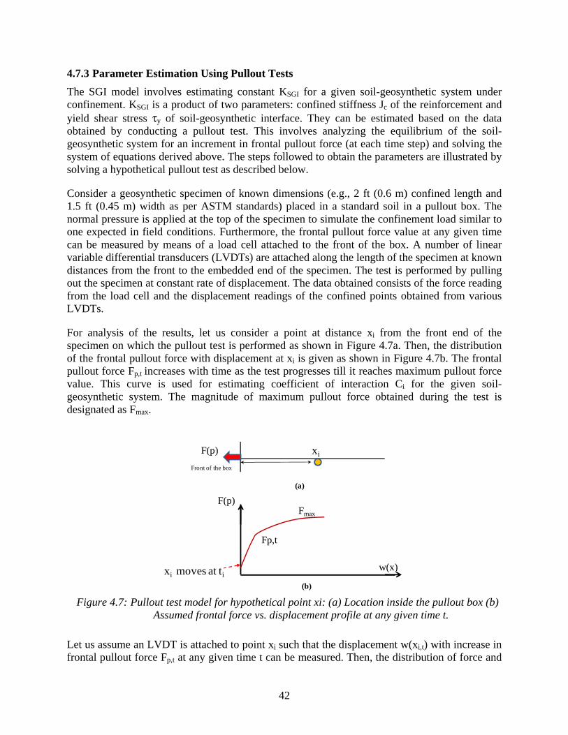
42

4.7.3 Parameter Estimation Using Pullout Tests

The SGI model involves estimating constant KSGI for a given soil-geosynthetic system under confinement. KSGI is a product of two parameters: confined stiffness Jc of the reinforcement and yield shear stress τy of soil-geosynthetic interface. They can be estimated based on the data obtained by conducting a pullout test. This involves analyzing the equilibrium of the soil-geosynthetic system for an increment in frontal pullout force (at each time step) and solving the system of equations derived above. The steps followed to obtain the parameters are illustrated by solving a hypothetical pullout test as described below.

Consider a geosynthetic specimen of known dimensions (e.g., 2 ft (0.6 m) confined length and 1.5 ft (0.45 m) width as per ASTM standards) placed in a standard soil in a pullout box. The normal pressure is applied at the top of the specimen to simulate the confinement load similar to one expected in field conditions. Furthermore, the frontal pullout force value at any given time can be measured by means of a load cell attached to the front of the box. A number of linear variable differential transducers (LVDTs) are attached along the length of the specimen at known distances from the front to the embedded end of the specimen. The test is performed by pulling out the specimen at constant rate of displacement. The data obtained consists of the force reading from the load cell and the displacement readings of the confined points obtained from various LVDTs.

For analysis of the results, let us consider a point at distance xi from the front end of the specimen on which the pullout test is performed as shown in Figure 4.7a. Then, the distribution of the frontal pullout force with displacement at xi is given as shown in Figure 4.7b. The frontal pullout force Fp,t increases with time as the test progresses till it reaches maximum pullout force value. This curve is used for estimating coefficient of interaction Ci for the given soil-geosynthetic system. The magnitude of maximum pullout force obtained during the test is designated as Fmax.

Figure 4.7: Pullout test model for hypothetical point xi: (a) Location inside the pullout box (b)

Assumed frontal force vs. displacement profile at any given time t.

Let us assume an LVDT is attached to point xi such that the displacement w(xi,t) with increase in frontal pullout force Fp,t at any given time t can be measured. Then, the distribution of force and

w(x)

xiF(p)

F(p)

xi moves at ti

Fp,t

Fmax

Front of the box

(a)

(b)

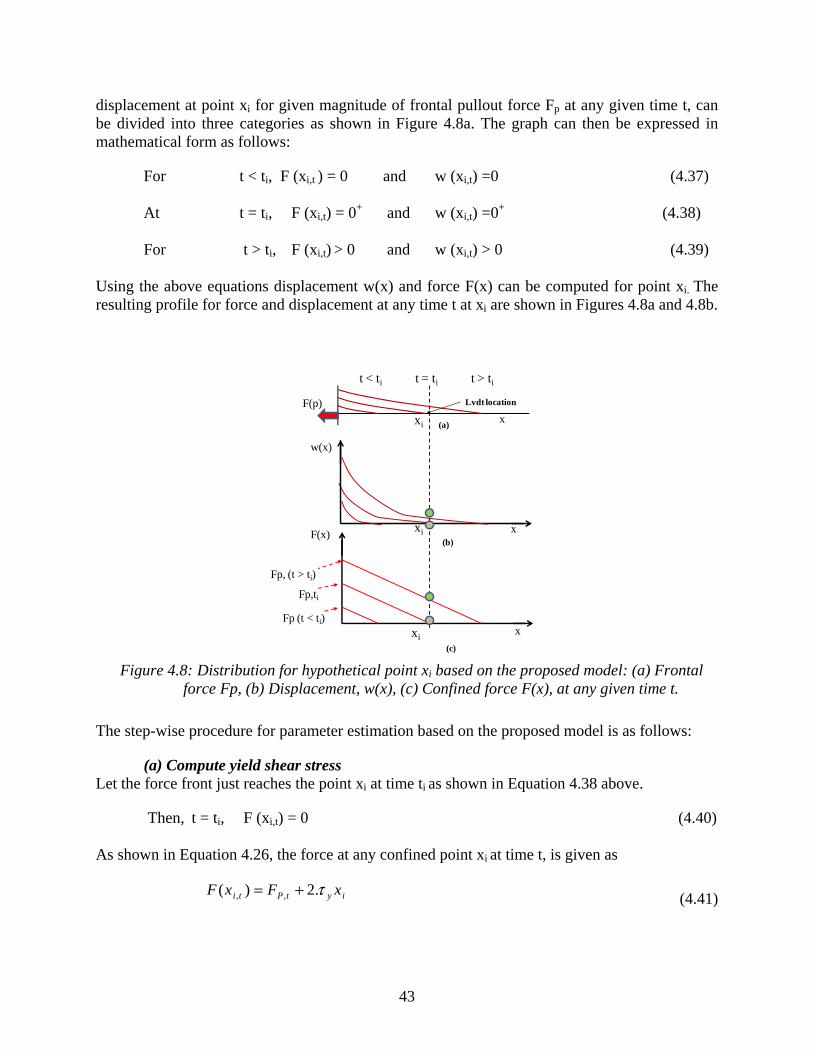
43

displacement at point xi for given magnitude of frontal pullout force Fp at any given time t, can be divided into three categories as shown in Figure 4.8a. The graph can then be expressed in mathematical form as follows:

For t < ti, F (xi,t ) = 0 and w (xi,t) =0 (4.37) At t = ti, F (xi,t) = 0+ and w (xi,t) =0+ (4.38) For t > ti, F (xi,t) > 0 and w (xi,t) > 0 (4.39)

Using the above equations displacement w(x) and force F(x) can be computed for point xi. The resulting profile for force and displacement at any time t at xi are shown in Figures 4.8a and 4.8b.

Figure 4.8: Distribution for hypothetical point xi based on the proposed model: (a) Frontal

force Fp, (b) Displacement, w(x), (c) Confined force F(x), at any given time t.

The step-wise procedure for parameter estimation based on the proposed model is as follows:

(a) Compute yield shear stress Let the force front just reaches the point xi at time ti as shown in Equation 4.38 above.

Then, t = ti, F (xi,t) = 0 (4.40) As shown in Equation 4.26, the force at any confined point xi at time t, is given as

iytPti xFxF τ.2)( ,, += (4.41)

t < ti t = ti t > ti

xxi(c)

(a)

w(x)

xF(x)

Fp, (t > ti)

Fp,ti

xi

F(p)

xi

Fp (t < ti)

(b)

Lvdt location

x

44

Substituting Equation 4.40 in Equation 4.41 above, yield shear stress at each point can be computed as follows;

i

tpy x

F

2,=τ (4.42)

If more than one LVDT is used during the test, then the value of τy can be calculated at each LVDT point and the average value can be used for the analysis. Because of the rigid-perfectly plastic assumption made for the behavior of the soil-geosynthetic interaction, the values of τy are expected to be similar at all the LVDT locations. Consequently, adopting an average τy value between subsequent LVDTs is considered a reasonable assumption. Also, as a first approximation τy value can be estimated knowing the maximum pullout force Fmax and total length of confined specimen, L;

L

Fy 2

max=τ (4.43)

The value of τy obtained using Equation 4.43 is generally higher than one calculated based on Equation 4.42 as the pullout force increases even after the entire length of the geosynthetic has been mobilized.

(b) Calculating confined force F (xi,t) at a point xi At any time t > ti, the confined force at the point xi is greater than zero. It can be calculated using Equation 4.41 because yield shear stress τy and frontal pullout force Fp,t are known;

iytPti xFxF τ.2)( ,, +=

Because an LVDT is attached to the point xi, the displacement w (xi,t) for a given frontal pullout force Fp,t is known. Then the results can be combined to plot the calculated confined force F (xi,t) vs. measured displacement w (xi,t) as shown in Figure 4.9a.

(c) Estimating confined stiffness, Jc Because the force and displacement at point xi are known and also yield stress τy, the Jc value can be directly obtained as shown in Figure 4.9b. It can be also calculated based on Equation 4.32.

)()...4()( ,2

, ticyti xwJxF τ= (4.44)

)(..4

)(

,

2,

tiy

tic xw

xFJ

τ=

(4.45)

45

Figure 4.9: Based on proposed model, for hypothetical point xi: (a) F (xi) vs. w (xi), (b) KSGI,

at any given time t.

(d) Computing coefficient of soil geosynthetic interaction, KSGI and equivalent confined modulus at a given displacement, MSGI

Knowing Jc and τy, KSGI value is calculated as follows:

cyiSGI JxK ..4)( τ= (4.46)

Then for any given displacement w (xi) (generally 0.04 in (1mm) for simplicity) MSGI can be calculated as follows:

)()(

..4

)(

)()(

,,,

,,

ti

SGI

ti

cy

ti

titiSGI xw

K

xw

J

xw

xFxM ===

τ

(4.47) The above procedure can be repeated for any instrumented point to obtain the coefficient of soil geosynthetic interaction from a pullout test.

(e) Check the estimated parameters Let us assume another point xj inside the pullout box such that an LVDT is attached to it. Then the value of w (xj) for a given Fp,t is known throughout the test. As τy and Jc were estimated from point xi, they can be used to predict the displacement profile at point xj using the Equation below.

cy

tPj

c

tPj

c

y

tj J

Fx

J

Fx

Jxw

..4..)(

2,,2

, ττ

++= (4.48)

Then the measured and predicted value of w (xj) can be compared to check the accuracy of estimated parameters; τy and Jc.

(f) Using regression analysis The data obtained from the pullout test can be used in a linear regression model to estimate the value of KSGI. The regression model can be setup by applying transformation to Equation 4.48 for all the LVDTs as follows:

332211 ...)( XXXXY βββ ++= (4.49) In the above model, Y(X) is the independent variable, X1, X2, X3 are the dependent variables and β1,, β2, β3 are the coefficients such that,

F(xi)

w(xi) w(xi)

KSGI= 4.τy.Jc

(b)(a)

F(xi)2

46

)()( ,tjxwXY = (4.50)

2

1 xX = (4.51)

jtP xFX .,2 = (4.52)

2

,3 tPFX = (4.53)

c

y

J

τβ =1 (4.54)

cJ

12 =β (4.55)

cy J..4

13 τ

β = (4.56)

The analytical model assumptions allow for regression analyses on data obtained during the test until maximum pullout force is reached. The inverse of coefficient β3 then gives the value of KSGI. This analysis helps to estimate bounds and confidence intervals on estimated value of KSGI. Furthermore, it can be compared with the value of KSGI obtained based on analytical solution proposed above.

4.7.4 Repeatability of the Estimated Parameter

Section 4.7.3 detailed the procedure to estimate the model parameters τy and Jc based on pullout test data. Specifically, it involved monitoring the frontal pullout force and displacement at a confined point inside the pullout box. The above analysis can be extended to any point inside the pullout box and the two model parameters can be obtained to compute the value of KSGI. This section discusses the repeatability of model parameters and KSGI for a given soil-geosynthetic system tested at given confining pressure in the pullout test. In other words, the value of KSGI is independent of the location of LVDT where displacement measurements are made during the pullout test.

Let us assume three instrumented points x1, x2, and x3 on a geosynthetic confined inside the pullout box as shown in Figure 4.10a. Then, Fp,t is the pullout force at any given time t and the maximum pullout force at the end of the test is Fmax. The variation of frontal pullout force with displacement at each instrumented point is as shown in Figure 4.10b. Based on the location of three points, the force front reaches them at different times. The point x1 is the closest to the pullout force end and thus experiences force and displacement earlier than x2, followed by x3. As the force front reaches the points x1, x2, and x3, they begin moving at times t1, t2, and t3 respectively. After the entire length of the geosynthetic is mobilized, the peak pullout force

47

magnitude Fmax is reached and there is no further change in the frontal pullout force with increase in the displacement of the points x1, x2, and x3.

Figure 4.10: Pullout test on a geosynthetic: (a) Instrumented points at distance x1, x2, and x3 (b)

Frontal pullout force vs. displacement profile for three points.

Then the data obtained from the pullout test can be analyzed based on the proposed model to obtain the displacement and force profile at any given time t for the entire length of the geosynthetic as shown in Figures 4.11a and 4.11b respectively.

Figure 4.11: Based on analysis of pullout test data, profiles at three points for any given time t:

(a) Displacement with length (b) Force with length.

Fp,t1

F(p)

w(x)x1 moves at t1

x2 moves at t2

x3 moves at t3

x1 x2 x3

F(p)

Fp,t3

Fp,t2

Fmax

(b)

(a)

w(x)

x

F(x)

x

Fp,t3

At t1

At t2

At t3

x1 x2 x3

Fp,t2

x1 x2 x3

Fp,t1

(a)

(b)

48

Then the information obtained above can be combined to plot the individual confined force vs. displacement profile at points x1, x2, and x3 as shown in Figure 4.12.

Figure 4.12: Confined force vs. measured displacement profile at point: (a) x1 (b) x2 (c) x3.

Furthermore, by solving the equations developed for the proposed model, the values of both parameters τy and Jc can be calculated at each of the three points x1, x2, and x3. Then the curves can be combined to get confined force vs. displacement relationship for the soil-geosynthetic system as shown in Figure 4.13a. Finally, as shown in Figure 4.13b, the value of soil-geosynthetic interaction coefficient for the entire test can be obtained. This value of KSGI appears to be unique for a given soil-geosynthetic system at a given confining pressure. Hence, it can be used as a parameter for predicting the performance of geosynthetics under confinement at low displacements as in the case of geosynthetic- reinforced pavements.

F(x1)

w(x1)

F(x2)

w(x2)

F(x3)

w(x3)

(a)

(c)

(b)

49

Figure 4.13: Plot for given soil-geosynthetic system at known confining pressure for all LVDTs

used during a test: (a) Confined force vs. displacement (b) KSGI

4.7.5 Discussion

The interpretation of the pullout test results based on an analytical model requires an accurate evaluation of the displacement and force distribution throughout the geosynthetic specimen at any time during the test. Section 4.7.4 listed the features of proposed analytical model to characterize the soil-geosynthetic interface properties at low displacements under confined conditions. Based on the analysis of the pullout test data a unique parameter KSGI can be calculated to quantify this behavior.

The proposed approach has advantages over available models as it uses only the pullout test data and makes realistic assumptions in solving the governing differential equation. Further, it allows for calculating a single value that can be used as the basis for comparing performance of two different types of geosynthetics, i.e., geogrids and geotextiles or similar products placed under same working conditions in the field. This approach is suitable for reinforced pavement design as it involves parameters that characterize the interaction under low displacements of the soil-geosynthetic interface.

F(x)

w(x)F(x)2

w(x)(b)

(a)

KSGI

1

50

51

Chapter 5. Pullout Test Results

5.1 Materials: Soils and Geosynthetics

5.1.1 Soils

Two types of soils were used, a sand and a gravel. The sand soil is the Monterrey No.30 sand (Figure 5.1), which was used for the initial baseline series of large pullout testing of geosynthetics and for the small pullout tests. The reason for this selection was the commercial availability of the soil and existing geotechnical database available to characterize the given soil. Furthermore, the volume of soil required to run a full scale pullout test was large, therefore the ease of handling of Monterey No. 30 sand in sample preparation and post-processing phase of the test made it a suitable choice.

Figure 5.1: Monterey No. 30 sand bags

Monterey No. 30 sand is clean uniformly graded sand classified as SP in the unified system and gradation curve of the soil is as shown in Figure 5.2. The particles are rounded to sub rounded consisting predominantly of quartz with a smaller amount of feldspar and other minerals (Zornberg, 1994).

Figure 5.2: Gradation curve of Monterey No. 30 sand (Li, 2005)

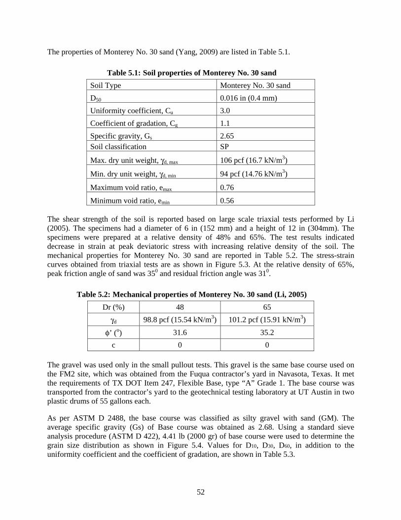
52

The properties of Monterey No. 30 sand (Yang, 2009) are listed in Table 5.1.

Table 5.1: Soil properties of Monterey No. 30 sand

Soil Type Monterey No. 30 sand

D50 0.016 in (0.4 mm)

Uniformity coefficient, Cu 3.0

Coefficient of gradation, Cg 1.1

Specific gravity, Gs 2.65 Soil classification SP

Max. dry unit weight, γd, max 106 pcf (16.7 kN/m3)

Min. dry unit weight, γd, min 94 pcf (14.76 kN/m3)

Maximum void ratio, emax 0.76

Minimum void ratio, emin 0.56 The shear strength of the soil is reported based on large scale triaxial tests performed by Li (2005). The specimens had a diameter of 6 in (152 mm) and a height of 12 in (304mm). The specimens were prepared at a relative density of 48% and 65%. The test results indicated decrease in strain at peak deviatoric stress with increasing relative density of the soil. The mechanical properties for Monterey No. 30 sand are reported in Table 5.2. The stress-strain curves obtained from triaxial tests are as shown in Figure 5.3. At the relative density of 65%, peak friction angle of sand was 350 and residual friction angle was 310.

Table 5.2: Mechanical properties of Monterey No. 30 sand (Li, 2005)

Dr (%) 48 65

γd 98.8 pcf (15.54 kN/m3) 101.2 pcf (15.91 kN/m3)

φ’ (o) 31.6 35.2

c 0 0

The gravel was used only in the small pullout tests. This gravel is the same base course used on the FM2 site, which was obtained from the Fuqua contractor’s yard in Navasota, Texas. It met the requirements of TX DOT Item 247, Flexible Base, type “A” Grade 1. The base course was transported from the contractor’s yard to the geotechnical testing laboratory at UT Austin in two plastic drums of 55 gallons each.

As per ASTM D 2488, the base course was classified as silty gravel with sand (GM). The average specific gravity (Gs) of Base course was obtained as 2.68. Using a standard sieve analysis procedure (ASTM D 422), 4.41 lb (2000 gr) of base course were used to determine the grain size distribution as shown in Figure 5.4. Values for D10, D30, D60, in addition to the uniformity coefficient and the coefficient of gradation, are shown in Table 5.3.

53

Figure 5.3: Results of triaxial compression test on Monterey No.30 sand: (a) deviatoric stress

and axial strain; (b) volumetric and axial strain; and (c) compression and volumetric strain, (Yang, 2009).

Based on the grain size distribution data presented in Table 5.3 and Figure 5.4, the values of Cc and Cu were calculated as shown in Table 5.4. As per ASTM D 2487, the base course was then classified as silty gravel with sand (GM-ML).

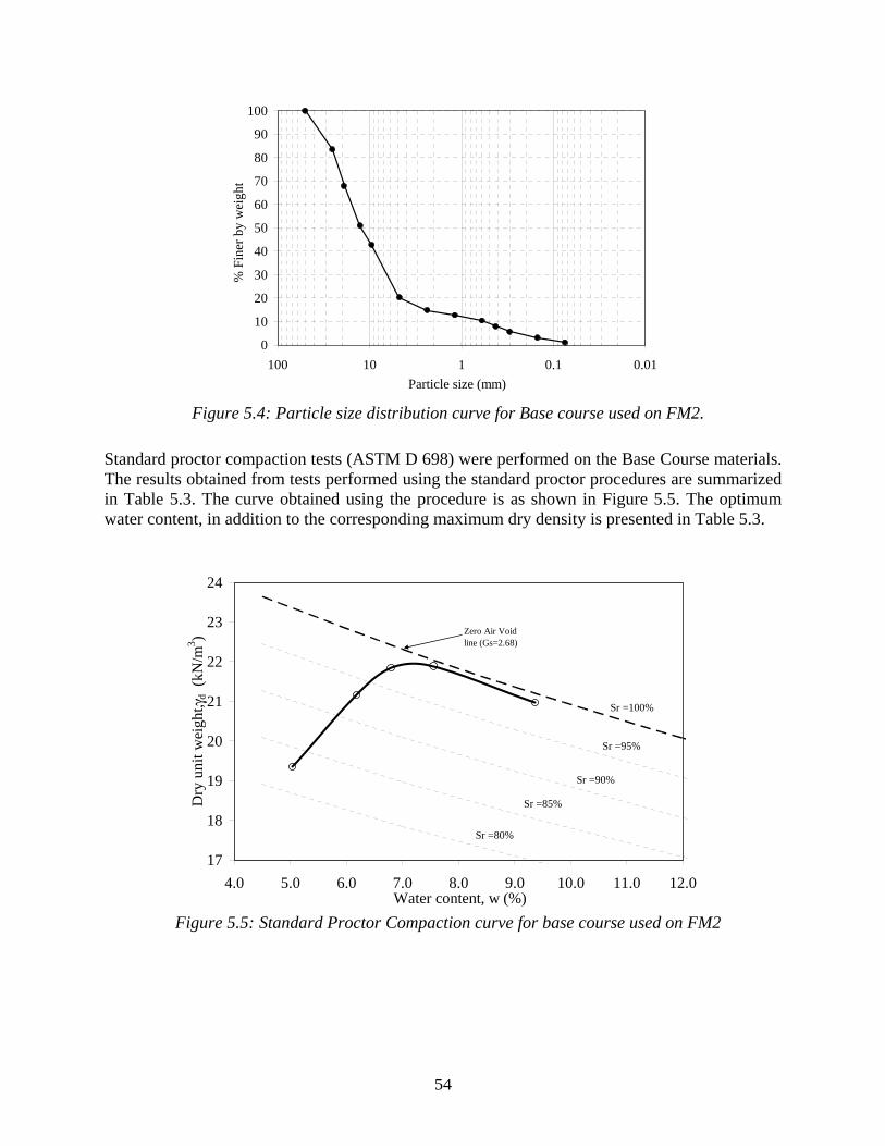
54

Figure 5.4: Particle size distribution curve for Base course used on FM2.

Standard proctor compaction tests (ASTM D 698) were performed on the Base Course materials. The results obtained from tests performed using the standard proctor procedures are summarized in Table 5.3. The curve obtained using the procedure is as shown in Figure 5.5. The optimum water content, in addition to the corresponding maximum dry density is presented in Table 5.3.

Figure 5.5: Standard Proctor Compaction curve for base course used on FM2

0

10

20

30

40

50

60

70

80

90

100

0.010.1110100

Particle size (mm)

% F

iner

by

wei

ght

17

18

19

20

21

22

23

24

4.0 5.0 6.0 7.0 8.0 9.0 10.0 11.0 12.0Water content, w (%)

Dry

uni

t wei

ght, γ

d (

kN/m

3 ) Zero Air Void line (Gs=2.68)

Sr =100%

Sr =80%

Sr =90%

Sr =95%

Sr =85%

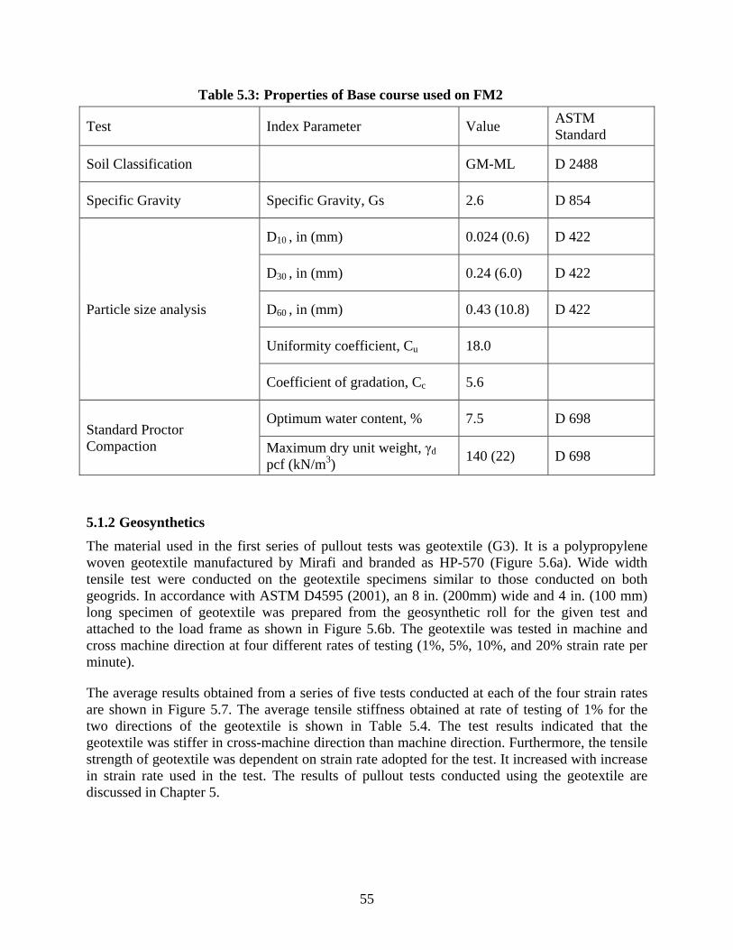
55

Table 5.3: Properties of Base course used on FM2

Test Index Parameter Value ASTM Standard

Soil Classification GM-ML D 2488

Specific Gravity Specific Gravity, Gs 2.6 D 854

Particle size analysis

D10 , in (mm) 0.024 (0.6) D 422

D30 , in (mm) 0.24 (6.0) D 422

D60 , in (mm) 0.43 (10.8) D 422

Uniformity coefficient, Cu 18.0

Coefficient of gradation, Cc 5.6

Standard Proctor Compaction

Optimum water content, % 7.5 D 698

Maximum dry unit weight, γd pcf (kN/m3)

140 (22) D 698

5.1.2 Geosynthetics

The material used in the first series of pullout tests was geotextile (G3). It is a polypropylene woven geotextile manufactured by Mirafi and branded as HP-570 (Figure 5.6a). Wide width tensile test were conducted on the geotextile specimens similar to those conducted on both geogrids. In accordance with ASTM D4595 (2001), an 8 in. (200mm) wide and 4 in. (100 mm) long specimen of geotextile was prepared from the geosynthetic roll for the given test and attached to the load frame as shown in Figure 5.6b. The geotextile was tested in machine and cross machine direction at four different rates of testing (1%, 5%, 10%, and 20% strain rate per minute).

The average results obtained from a series of five tests conducted at each of the four strain rates are shown in Figure 5.7. The average tensile stiffness obtained at rate of testing of 1% for the two directions of the geotextile is shown in Table 5.4. The test results indicated that the geotextile was stiffer in cross-machine direction than machine direction. Furthermore, the tensile strength of geotextile was dependent on strain rate adopted for the test. It increased with increase in strain rate used in the test. The results of pullout tests conducted using the geotextile are discussed in Chapter 5.

56

Figure 5.6: Geosynthetic used for baseline tests (a) Geotextile (G3); (b) specimen used in wide-

width tensile test

Figure 5.7: Wide width tensile test results for geotextile at different strain rates (a) Machine

direction (b) Cross-Machine direction

Table 5.4: Wide width tensile tests results for the geotextile

Properties Units 1% strain per minute

MD XD

Stiffness at 1% strain kip/ft (kN/m) 42.3 (618) 56.5 (825)

Stiffness at 2% strain kip/ft (kN/m) 40.7 (595) 47.7 (697)

Stiffness at 5% strain kip/ft (kN/m) 32.1 (469) 33.3 (487)

Stiffness at 10% strain kip/ft (kN/m) 29.2 (426) 26.2 (383)

Stiffness at maximum load kip/ft (kN/m) 26.6 (389) 21.0 (307)

Strain at maximum load % 20 20

The two geogrid products used in this test series (Tensar BX-1100 (G1) and Tensar BX-1200 (G4), Figure 5.8) were obtained from Tensar Earth Technologies. Geogrid G1 was used in the preliminary series of the testing program as described in Chapter 3. It was decided to compare its performance with another geogrid product that had similar physical properties but was reportedly

57

used for conditions that require better performance. Therefore, geogrid G4 was obtained from the same manufacturer to evaluate the properties of both geosynthetics under pullout conditions to validate the proposed model. These geogrids are marketed for the pavement reinforcement purposes, with geogrid G4 being considered superior in performance to G1. Evaluation of the KSGI value for these a product reportedly of better performance (G4) was expected to lead to a higher value of KSGI.

Figure 5.8: Geogrids: (a) Tensar BX-1100 (G1); (b) Tensar BX 1200 (G4) (adapted from

Finnefrock, 2008)

The two geogrids have similar physical properties. Both these geogrids are integrally formed, punched-and-drawn polypropylene (PP) grids featuring raised protrusions at each rib intersections to provide a structural abutment when placed between soil layers. They have similar physical dimensions—i.e., aperture size and rib shape. The major difference between the two geogrids is the unconfined tensile strength, with the BX-1200 having a higher tensile strength in both machine and cross-machine directions than BX-1100. The index values of both products as reported by Tensar (2002) are listed in Table 5.5.

The geosynthetic G2 is a Mirafi BasX-11 geogrid as shown in Figure 5.9. The geogrid has an aperture size of 1 in (25 mm) in both machine and cross-machine direction. The manufacturer reported similar tensile strength in the machine and cross-machine direction for geogrid G2 (1.98 kip/ft (29 kN/m)). The manufacturing process involved in this geogrid is different from geogrids used in test series-II of this implementation project.

The geogrid G2 differs from geogrid G1 as it has no distinct protrusions at the junction of longitudinal and transverse ribs. The geogrid G2 has similar properties in both principal directions whereas G1 had stronger cross-machine direction than machine direction. However, the unconfined tensile strength of geogrid G2 was greater than G1 in both directions.

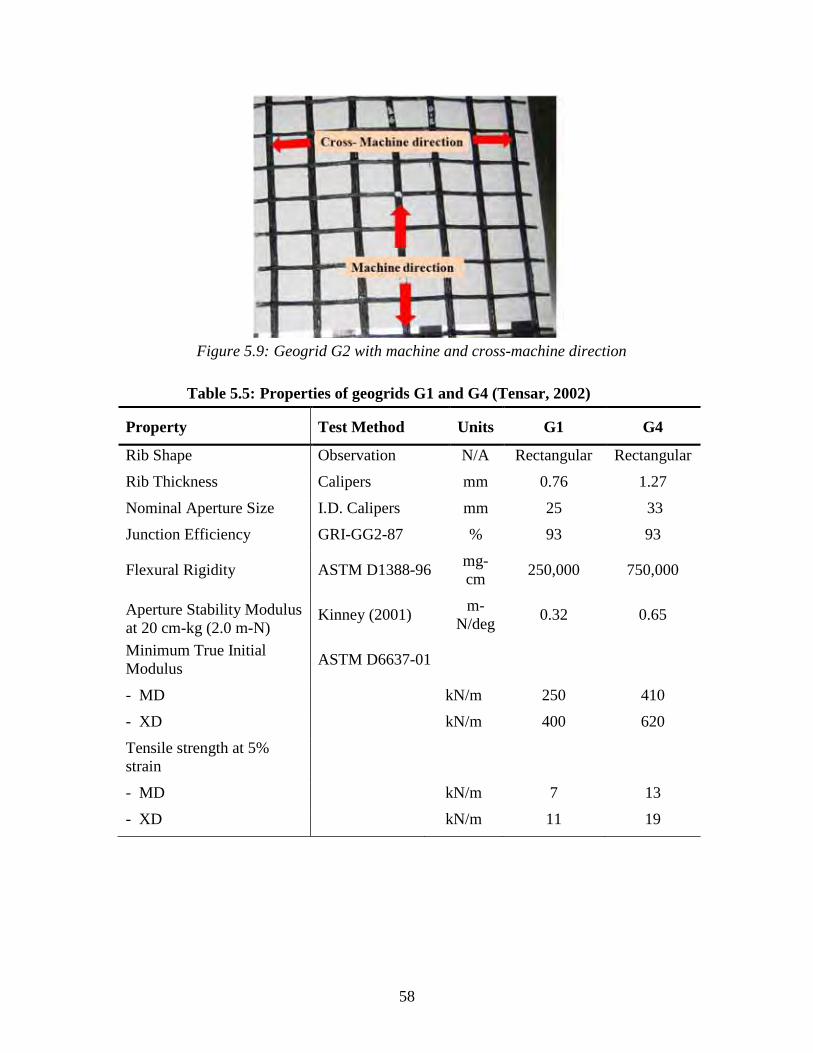
58

Figure 5.9: Geogrid G2 with machine and cross-machine direction

Table 5.5: Properties of geogrids G1 and G4 (Tensar, 2002)

Property Test Method Units G1 G4

Rib Shape Observation N/A Rectangular Rectangular

Rib Thickness Calipers mm 0.76 1.27

Nominal Aperture Size I.D. Calipers mm 25 33

Junction Efficiency GRI-GG2-87 % 93 93

Flexural Rigidity ASTM D1388-96 mg-cm

250,000 750,000

Aperture Stability Modulus at 20 cm-kg (2.0 m-N)

Kinney (2001) m-

N/deg0.32 0.65

Minimum True Initial Modulus

ASTM D6637-01

- MD kN/m 250 410

- XD kN/m 400 620

Tensile strength at 5% strain

- MD kN/m 7 13

- XD kN/m 11 19

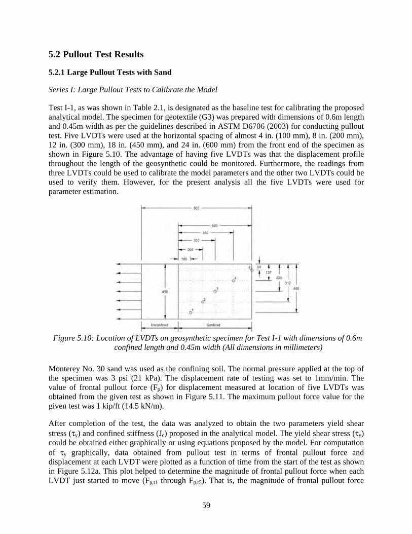
59

5.2 Pullout Test Results

5.2.1 Large Pullout Tests with Sand

Series I: Large Pullout Tests to Calibrate the Model

Test I-1, as was shown in Table 2.1, is designated as the baseline test for calibrating the proposed analytical model. The specimen for geotextile (G3) was prepared with dimensions of 0.6m length and 0.45m width as per the guidelines described in ASTM D6706 (2003) for conducting pullout test. Five LVDTs were used at the horizontal spacing of almost 4 in. (100 mm), 8 in. (200 mm), 12 in. (300 mm), 18 in. (450 mm), and 24 in. (600 mm) from the front end of the specimen as shown in Figure 5.10. The advantage of having five LVDTs was that the displacement profile throughout the length of the geosynthetic could be monitored. Furthermore, the readings from three LVDTs could be used to calibrate the model parameters and the other two LVDTs could be used to verify them. However, for the present analysis all the five LVDTs were used for parameter estimation.

Figure 5.10: Location of LVDTs on geosynthetic specimen for Test I-1 with dimensions of 0.6m

confined length and 0.45m width (All dimensions in millimeters)

Monterey No. 30 sand was used as the confining soil. The normal pressure applied at the top of the specimen was 3 psi (21 kPa). The displacement rate of testing was set to 1mm/min. The value of frontal pullout force (Fp) for displacement measured at location of five LVDTs was obtained from the given test as shown in Figure 5.11. The maximum pullout force value for the given test was 1 kip/ft (14.5 kN/m).

After completion of the test, the data was analyzed to obtain the two parameters yield shear stress (τy) and confined stiffness (Jc) proposed in the analytical model. The yield shear stress (τy) could be obtained either graphically or using equations proposed by the model. For computation of τy graphically, data obtained from pullout test in terms of frontal pullout force and displacement at each LVDT were plotted as a function of time from the start of the test as shown in Figure 5.12a. This plot helped to determine the magnitude of frontal pullout force when each LVDT just started to move (Fp,t1 through Fp,t5). That is, the magnitude of frontal pullout force

60

corresponding to the active length of reinforcement was defined. Then, these values were plotted against the location of each LVDT on the geosynthetic specimen as shown in Figure 5.12b.

Figure 5.11: Frontal pullout force vs. displacement curve for each LVDT

Figure 5.12: Computation of yield shear stress parameter graphically (a) Frontal pullout force

and displacement as function of time from start of test; (b) Frontal pullout force vs. active length of the reinforcement

0.0

2.5

5.0

7.5

10.0

12.5

15.0

0 1 2 3 4 5 6 7 8 9 10

Fro

ntal

pul

lout

forc

e, F

P(k

N/m

)

Displacement , w(x) mm

1

4

Fmax

32

5

0

1

2

3

4

5

6

7

8

9

10

0.0

2.5

5.0

7.5

10.0

12.5

15.0

0 180 360 540 720 900 1080 1260 1440

Dis

plac

emen

t, w

(x)

mm

Fro

ntal

pul

lout

forc

e,F p

(kN

/m)

time, t sec

Fp,t1

Fp,t2

Fp,t3

Fp,t4

Fp,t5

d1

d2d3

d4

d5

y = 21.1xR² = 0.95

0.0

2.5

5.0

7.5

10.0

12.5

15.0

0.00 0.05 0.10 0.15 0.20 0.25 0.30 0.35 0.40 0.45 0.50 0.55 0.60

Fron

tal p

ullo

ut fo

rce,

Fp

(kN

/m)

Mobilized length, L' (m)

LVDT 1 LVDT 4LVDT 3LVDT 2 LVDT 5

τy = 21.1/2 = 10.5 kN/m2

Equation for trendline

Yield shear stress

(a)

(b)

61

The line was then fitted through these points and its slope was determined. Because shear stress is mobilized on top and bottom of the specimen, its value was half of the value obtained from slope of the curve. The yield shear stress (τy) for the given soil-geosynthetic system was calculated as 219 psf (10.5 kN/m2).

Alternatively, the magnitude of frontal pullout force at which each individual LVDT starts moving can be determined from the test data. At this frontal pullout force, the active length of reinforcement is known and is equal to the location where the LVDT was placed before the start of test. Thus, the value of yield shear stress can be calculated using Equation 4.43 as shown in Table 5.6.

Table 5.6: Computation for yield shear stress

LVDT Number

Location from front end, L′

Time to start of displacement

Force Fp

Yield Shear τy=Fp/2L′

mm seconds kip/ft (kN/m) psf (kN/m2)

1 100 466 0.21 (3.0) 313 (15)

2 200 562 0.38 (5.5) 271 (13)

3 300 669 0.47 (6.8) 229 (11)

4 450 820 0.63 (9.19) 209 (10)

5 600 1014 0.83 (12.22) 229 (11)

The present model assumed a constant value of τy throughout the geosynthetic specimen for the given test. However, in the above analysis, the first LVDT had higher shear stress value and last two LVDTs have lower values than those obtained from middle LVDTs. Thus, it can be seen that yield shear stress was influenced by the boundary conditions. Theoretically, the results from the LVDT located in the very middle of the specimen, could be the best estimate for τy. However, in reality many factors can locally affect the results of the middle LVDT. Therefore, for calculation purposes, an average value of τy was assumed for the entire test for a given soil-geosynthetic system subjected to a known normal pressure. Because of edge effects are expected to affect primarily the data collected using LVDTs 1 and 5, averages using the data from LVDTs 2, 3, and 4 are considered a better estimate of τy.

To compute the value of confined stiffness (Jc), it was necessary to obtain the confined force and displacement response at each LVDT. Therefore, after computing the yield shear stress τy, the confined force F(x) at LVDT point xi, for a given frontal pullout force Fp was estimated as shown in Equation 5.1 as,

(5.1)

The confined force F(x) and displacement w(x) at each of the five LVDT points is shown in Figure 5.13. The LVDTs 2 and 3, which are in the middle of the geosynthetic specimen, were least influenced by the boundary conditions and had similar confined force and displacement

iyPi xFxF τ.2)( +=

62

response. This trend was as hypothesized by in the development of the analytical model, where it was suggested that the confined force and displacement response is unique for a given soil-geosynthetic system.

Figure 5.13: Confined force vs. displacement curve for baseline test

The next step in the analysis involved determining the magnitude of the confined stiffness (Jc) for the given system. It could be estimated graphically by plotting the square of the confined force at a point vs. displacement at that point as shown in Figure 5.14. Then, the slope of this curve directly gives the value of constant KSGI, which can be used to back-calculate the value of Jc for a given average value of τy using Equation 5.1. This graphical method was used in the present analysis to estimate this parameter.

(5.2)

Alternatively, Jc could be computed by using Equation 4.45 shown below for a given value of confined force and displacement at a point.

(5.3)

The average value of confined stiffness based on the data obtained from LVDT 2 (at 0.04 in (1 mm) displacement) was estimated at 40.4 kip/ft (590 kN/m).

0.0

2.5

5.0

7.5

10.0

12.5

15.0

0.0 0.5 1.0 1.5 2.0 2.5 3.0 3.5 4.0 4.5 5.0

Con

fine

d F

orce

F(x

), k

N/m

Displacement w(x),mm

1

43

2

5

y

SGIc

KJ

τ.4=

)(..4

)( 2

iy

ic xw

xFJ

τ=

63

Figure 5.14: Estimating KSGI graphically

Alternatively, after computing the value of two model parameters (knowing the τy and Jc magnitude mathematically), the value of KSGI could be obtained using Equation 4.46. For the given test, KSGI was estimated at 24990 kN2/m3 (or 24.9(kN/m)2/mm). The above value of KSGI can also be converted to equivalent modulus MSGI at 0.04 in (1 mm) displacement using the Equation 4.47, which was given as,

(5.4)

Finally, the prediction of the pullout force and displacement based on estimated parameters τy and Jc were compared with that measured during the test at all the five locations using the Equation 4.48.

cy

tPj

c

tPj

c

y

tj J

Fx

J

Fx

Jxw

..4..)(

2,,2

, ττ

++=

The curve showing the predicted vs. measured displacement is shown in Figure 5.15. Good agreement was obtained between the measured and predicted values of frontal pullout force and LVDT displacements at five LVDT locations in terms of two model parameters.

The regression analysis was conducted on the data obtained from the pullout test to directly obtain the KSGI value as discussed in Section 4.7.3. Furthermore, the upper and lower bounds on the estimates of KSGI were established as shown in Table 5.7. Based on these results it was estimated that the variation in KSGI value for a given test is within 1000 (kN/m)2/m for 95% upper and lower bound interval.

0

25

50

75

100

125

150

0 1 2 3 4 5 6

Con

fine

d F

orce

F(x

)2 ,[ k

N/m

]2

Displacement w(x),mm

KSGI=4.τy.Jc

1

2/50001000/1

24990

)()( mkN

xw

KxM

i

SGIiSGI ≅==

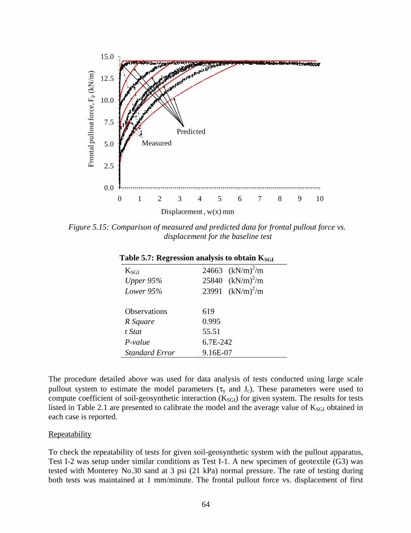
64

Figure 5.15: Comparison of measured and predicted data for frontal pullout force vs.

displacement for the baseline test

Table 5.7: Regression analysis to obtain KSGI

The procedure detailed above was used for data analysis of tests conducted using large scale pullout system to estimate the model parameters (τy and Jc). These parameters were used to compute coefficient of soil-geosynthetic interaction (KSGI) for given system. The results for tests listed in Table 2.1 are presented to calibrate the model and the average value of KSGI obtained in each case is reported.

Repeatability

To check the repeatability of tests for given soil-geosynthetic system with the pullout apparatus, Test I-2 was setup under similar conditions as Test I-1. A new specimen of geotextile (G3) was tested with Monterey No.30 sand at 3 psi (21 kPa) normal pressure. The rate of testing during both tests was maintained at 1 mm/minute. The frontal pullout force vs. displacement of first

0.0

2.5

5.0

7.5

10.0

12.5

15.0

0 1 2 3 4 5 6 7 8 9 10

Fro

ntal

pul

lout

forc

e, F

P(k

N/m

)

Displacement , w(x) mm

Measured

Predicted

KSGI 24663 (kN/m)2/m Upper 95% 25840 (kN/m)2/m Lower 95% 23991 (kN/m)2/m

Observations 619 R Square 0.995 t Stat 55.51 P-value 6.7E-242 Standard Error 9.16E-07

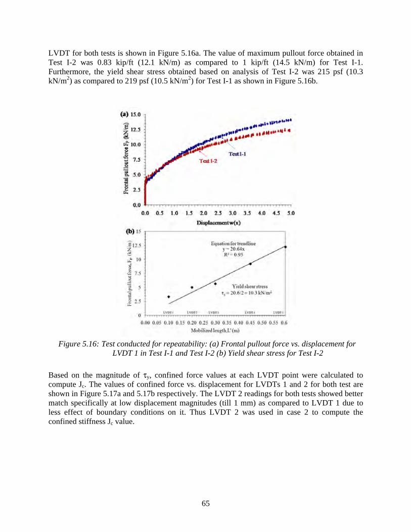
65

LVDT for both tests is shown in Figure 5.16a. The value of maximum pullout force obtained in Test I-2 was 0.83 kip/ft (12.1 kN/m) as compared to 1 kip/ft (14.5 kN/m) for Test I-1. Furthermore, the yield shear stress obtained based on analysis of Test I-2 was 215 psf (10.3 kN/m2) as compared to 219 psf (10.5 kN/m2) for Test I-1 as shown in Figure 5.16b.

Figure 5.16: Test conducted for repeatability: (a) Frontal pullout force vs. displacement for

LVDT 1 in Test I-1 and Test I-2 (b) Yield shear stress for Test I-2

Based on the magnitude of τy, confined force values at each LVDT point were calculated to compute Jc. The values of confined force vs. displacement for LVDTs 1 and 2 for both test are shown in Figure 5.17a and 5.17b respectively. The LVDT 2 readings for both tests showed better match specifically at low displacement magnitudes (till 1 mm) as compared to LVDT 1 due to less effect of boundary conditions on it. Thus LVDT 2 was used in case 2 to compute the confined stiffness Jc value.

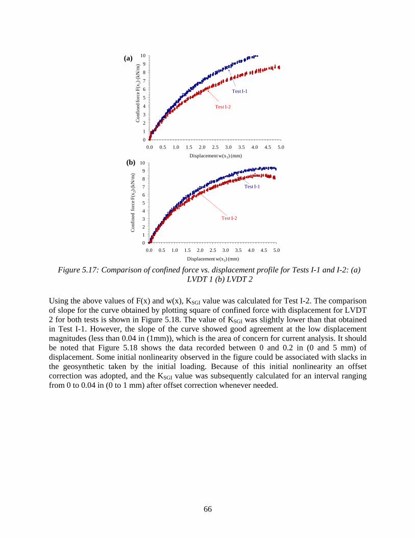
66

Figure 5.17: Comparison of confined force vs. displacement profile for Tests I-1 and I-2: (a)

LVDT 1 (b) LVDT 2

Using the above values of F(x) and w(x), KSGI value was calculated for Test I-2. The comparison of slope for the curve obtained by plotting square of confined force with displacement for LVDT 2 for both tests is shown in Figure 5.18. The value of KSGI was slightly lower than that obtained in Test I-1. However, the slope of the curve showed good agreement at the low displacement magnitudes (less than 0.04 in (1mm)), which is the area of concern for current analysis. It should be noted that Figure 5.18 shows the data recorded between 0 and 0.2 in (0 and 5 mm) of displacement. Some initial nonlinearity observed in the figure could be associated with slacks in the geosynthetic taken by the initial loading. Because of this initial nonlinearity an offset correction was adopted, and the KSGI value was subsequently calculated for an interval ranging from 0 to 0.04 in (0 to 1 mm) after offset correction whenever needed.

0

1

2

3

4

5

6

7

8

9

10

0.0 0.5 1.0 1.5 2.0 2.5 3.0 3.5 4.0 4.5 5.0

Con

fine

d f

orce

F(x

2) (k

N/m

)

Displacement w(x2) (mm)

Test I-2

Test I-1

0

1

2

3

4

5

6

7

8

9

10

0.0 0.5 1.0 1.5 2.0 2.5 3.0 3.5 4.0 4.5 5.0

Con

fine

d fo

rce

F(x 1

) (k

N/m

)

Displacement w(x1) (mm)

Test I-2

Test I-1

(a)

(b)

67

Figure 5.18: Comparison of KSGI values obtained for Tests I-1 and I-2 graphically

The average values of each parameter for both tests are reported in Table 5.8. The results obtained from both the tests indicated less variability in the model parameters (i.e., Jc, τy and KSGI) when compared to pullout test parameters (i.e., Fmax and τmax). Also, the value of KSGI from both tests were comparable and within the range of confidence intervals as determined in the previous case. Note that, KSGI, τy, and Jc can be considered small displacement parameters. This is because KSGI and τy are measured at small displacements values and Jc is determined by dividing KSGI by 4τy. On the other hand, Fmax and τmax are determined at the end of the pullout test, i.e., after the failure, when large displacements have developed.

Table 5.8: Repeatability of test results

Effect of Specimen Length

The effect of change in specimen length was quantified by conducting tests at two different specimen lengths of 0.9m and 0.3m from the baseline specimen length of 0.6m. The width of specimen in all these tests was 0.45m. The LVDTs were relocated on both specimens in Test I-3 (3 ft (0.9 m) long) and Test I-4 (1 ft (0.3 m) long) as shown in Figure 5.19a and 5.19b respectively. The tests were conducted by applying a normal pressure of 3 psi (21 kPa) on the top of soil-geosynthetic specimen.

The frontal pullout force values corresponding to displacements for the four tests (Test I-1, I-2, I-3, and I-4) are plotted for LVDT locations 1 and 2 as shown in Figure 5.20a and 5.21b. Based on the results obtained from these tests it was observed that the maximum pullout force increased with the increase in the length of the specimen for the same width.

0

10

20

30

40

50

60

70

80

90

100

0.0 0.5 1.0 1.5 2.0 2.5 3.0 3.5 4.0 4.5 5.0

Con

fine

d f

orce

F(x

2)2

(kN

/m)

Displacement w(x2) (mm)

Test I-2

Test I-1KSGI

Test Specimen dim. Pullout parameters Model parameters Constant L W Fmax τmax Jc τy KSGI MSGI,1mm m m kN/m kN/m2 kN/m kN/m2 (kN/m)2/m kN/m2

I-1 0.60 0.45 14.5 12.1 590 10.5 24780 4978 I-2 0.60 0.45 12.1 10.1 570 10.3 23484 4846

68

The results were used to compute the value of the yield shear stress for Tests I-3 and I-4 as shown in Figure 5.21a and 5.21b respectively. In Test I-3, due to increase in the length of the test specimen, the front of the specimen was stretched (extensibility) before the force reached its back end, thereby causing non-uniform yield shear stress distribution in the specimen close to maximum pullout resistance value. Thus the model assumptions were not valid in this range of pullout force. This can be seen for LVDT 5 in Test I-3, which moved at lower shear stress value that the rest of the specimen. Thus, it was not used to compute τy value. Further, this also indicated there is limiting value of specimen length for which model assumptions are valid at a given confining pressure.

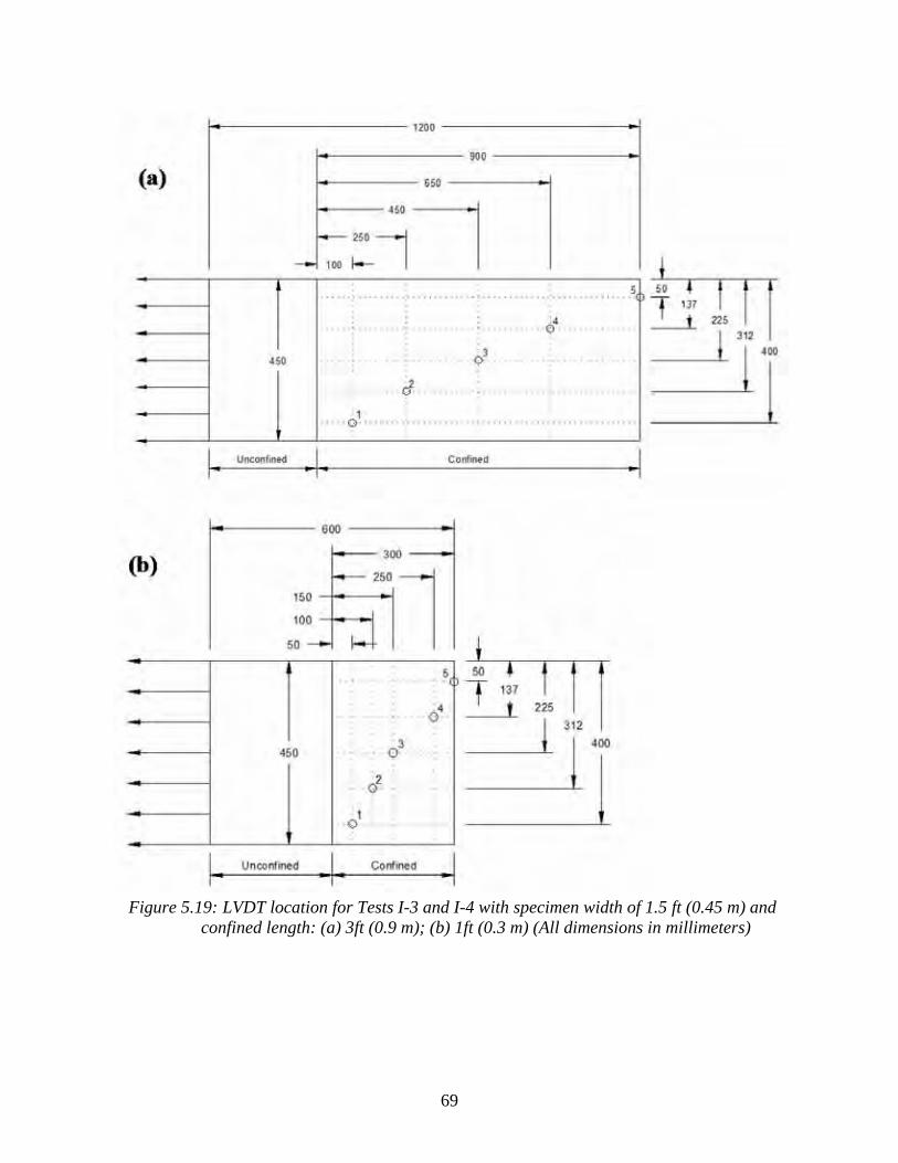
69

Figure 5.19: LVDT location for Tests I-3 and I-4 with specimen width of 1.5 ft (0.45 m) and

confined length: (a) 3ft (0.9 m); (b) 1ft (0.3 m) (All dimensions in millimeters)

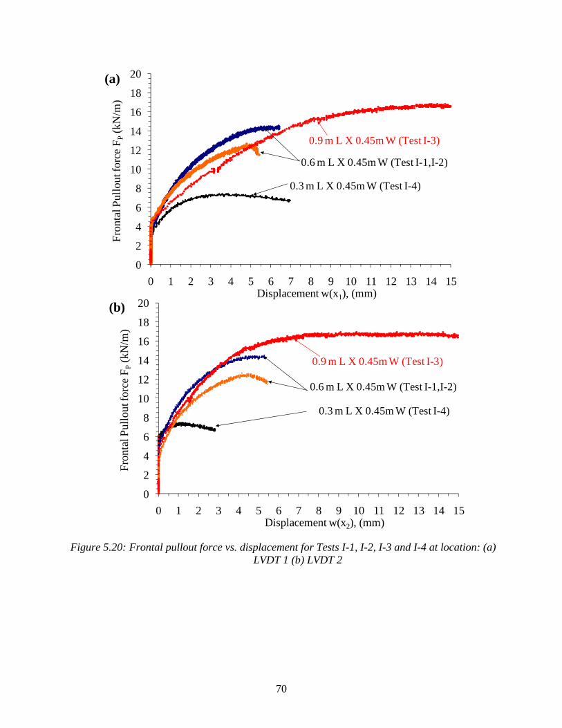
70

Figure 5.20: Frontal pullout force vs. displacement for Tests I-1, I-2, I-3 and I-4 at location: (a)

LVDT 1 (b) LVDT 2

0

2

4

6

8

10

12

14

16

18

20

0 1 2 3 4 5 6 7 8 9 10 11 12 13 14 15

Fro

ntal

Pul

lout

forc

e F

P(k

N/m

)

Displacement w(x1), (mm)

0.3 m L X 0.45m W (Test I-4)

0.9 m L X 0.45m W (Test I-3)

0.6 m L X 0.45m W (Test I-1,I-2)

0

2

4

6

8

10

12

14

16

18

20

0 1 2 3 4 5 6 7 8 9 10 11 12 13 14 15

Fro

ntal

Pul

lout

forc

e F

P(k

N/m

)

Displacement w(x2), (mm)

0.3 m L X 0.45m W (Test I-4)

0.9 m L X 0.45m W (Test I-3)

0.6 m L X 0.45m W (Test I-1,I-2)

(a)

(b)

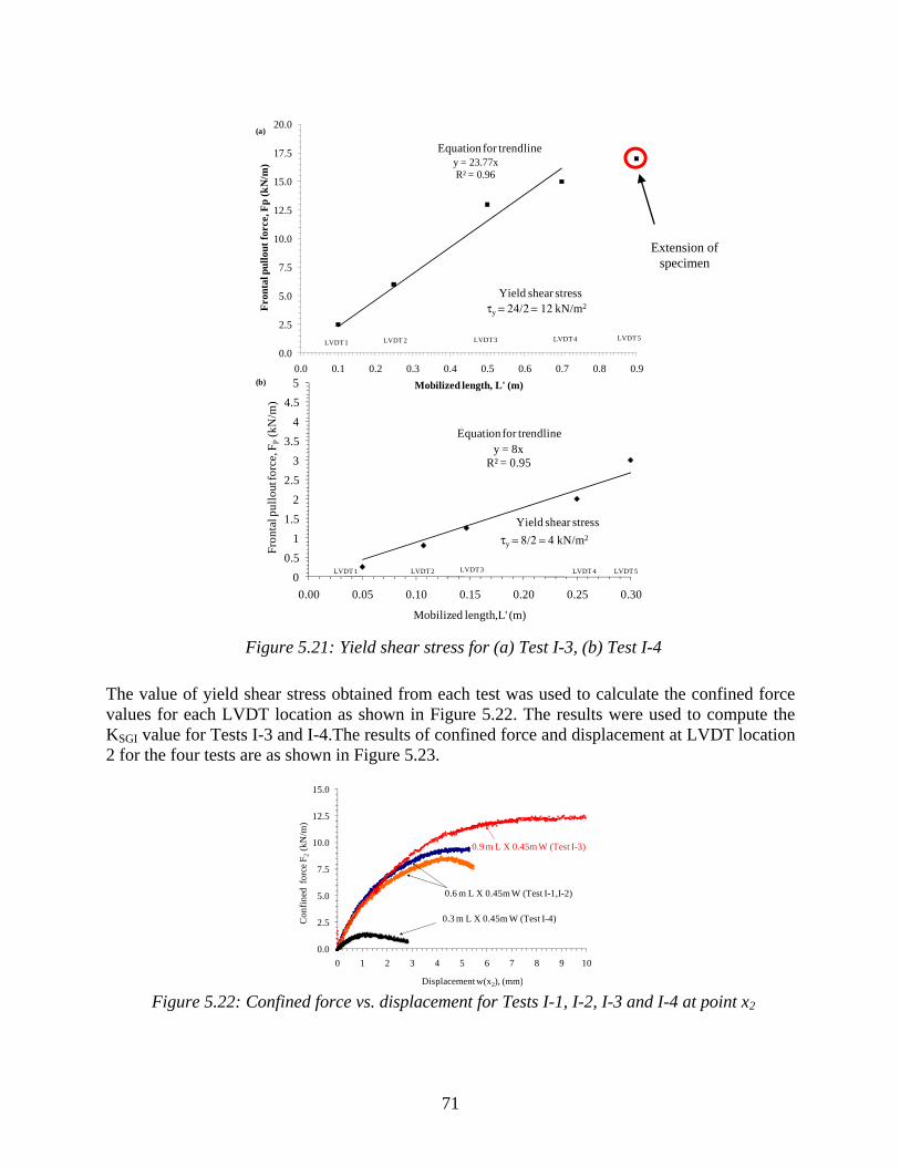
71

Figure 5.21: Yield shear stress for (a) Test I-3, (b) Test I-4

The value of yield shear stress obtained from each test was used to calculate the confined force values for each LVDT location as shown in Figure 5.22. The results were used to compute the KSGI value for Tests I-3 and I-4.The results of confined force and displacement at LVDT location 2 for the four tests are as shown in Figure 5.23.

Figure 5.22: Confined force vs. displacement for Tests I-1, I-2, I-3 and I-4 at point x2

y = 23.77xR² = 0.96

0.0

2.5

5.0

7.5

10.0

12.5

15.0

17.5

20.0

0.0 0.1 0.2 0.3 0.4 0.5 0.6 0.7 0.8 0.9

Fro

ntal

pul

lout

for

ce, F

p (k

N/m

)

Mobilized length, L' (m)

τy = 24/2 = 12 kN/m2

Equation for trendline

Yield shear stress

LVDT 1 LVDT 4LVDT 3LVDT 2 LVDT 5

y = 8xR² = 0.95

0

0.5

1

1.5

2

2.5

3

3.5

4

4.5

5

0.00 0.05 0.10 0.15 0.20 0.25 0.30

Fro

ntal

pul

lout

forc

e, F

P(k

N/m

)

Mobilized length,L' (m)

LVDT 1 LVDT 4LVDT 3LVDT 2 LVDT 5

τy = 8/2 = 4 kN/m2

Equation for trendline

Yield shear stress

(a)

(b)

0.0

2.5

5.0

7.5

10.0

12.5

15.0

0 1 2 3 4 5 6 7 8 9 10

Con

fine

d f

orce

F2

(kN

/m)

Displacement w(x2), (mm)

0.3 m L X 0.45m W (Test I-4)

0.9 m L X 0.45m W (Test I-3)

0.6 m L X 0.45m W (Test I-1,I-2)

Extension of specimen

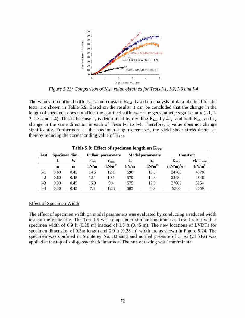
72

Figure 5.23: Comparison of KSGI value obtained for Tests I-1, I-2, I-3 and I-4

The values of confined stiffness Jc and constant KSGI, based on analysis of data obtained for the tests, are shown in Table 5.9. Based on the results, it can be concluded that the change in the length of specimen does not affect the confined stiffness of the geosynthetic significantly (I-1, I-2, I-3, and I-4). This is because Jc is determined by dividing KSGI by 4τy, and both KSGI and τy change in the same direction in each of Tests I-1 to I-4. Therefore, Jc value does not change significantly. Furthermore as the specimen length decreases, the yield shear stress decreases thereby reducing the corresponding value of KSGI.

Table 5.9: Effect of specimen length on KSGI

Effect of Specimen Width

The effect of specimen width on model parameters was evaluated by conducting a reduced width test on the geotextile. The Test I-5 was setup under similar conditions as Test I-4 but with a specimen width of 0.9 ft (0.28 m) instead of 1.5 ft (0.45 m). The new locations of LVDTs for specimen dimension of 0.3m length and 0.9 ft (0.28 m) width are as shown in Figure 5.24. The specimen was confined in Monterey No. 30 sand and normal pressure of 3 psi (21 kPa) was applied at the top of soil-geosynthetic interface. The rate of testing was 1mm/minute.

0

10

20

30

40

50

60

70

80

90

100

0 1 2 3 4 5

Con

fine

d f

orce

F22

(kN

/m)2

Displacement w(x2),mm

0.3 m L X 0.45m W (Test I-4)

0.9 m L X 0.45m W (Test I-3)

0.6 m L X 0.45m W (Test I-1, I-2)

Test Specimen dim. Pullout parameters Model parameters Constant L W Fmax τmax Jc τy KSGI MSGI,1mm

m m kN/m kN/m2 kN/m kN/m2 (kN/m)2/m kN/m2 I-1 0.60 0.45 14.5 12.1 590 10.5 24780 4978 I-2 0.60 0.45 12.1 10.1 570 10.3 23484 4846 I-3 0.90 0.45 16.9 9.4 575 12.0 27600 5254 I-4 0.30 0.45 7.4 12.3 585 4.0 9360 3059

73

Figure 5.24: LVDT locations for Test I-5 with confined length of 0.3m and width of 0.28m (All

dimension in millimeters)

The comparison of results obtained for frontal pullout force from LVDT 1 for Test I-4 and I-5 is shown in Figure 5.25. The maximum pullout force magnitude obtained in Test I-5 had a value of 0.6 kip/ft (8.7 kN/m), which was greater than value of 0.51 kip/ft (7.4 kN/m) obtained for Test I-4. Thus, reducing the width of the geosynthetic specimen for similar test conditions in a pullout box lead to its stiffer response in term of pullout resistance.

Figure 5.25: Comparison of frontal pullout force vs. displacement response for Tests I-4 and I-5

Similar observations were made by theoretical and experimental studies carried out by Hayashi et al. (1996) and Ghionna et al. (2001). They showed that for geosynthetic specimens having a width smaller than the pullout box, a three-dimensional soil dilatancy effect develops. The non-dilating zones in the soil surrounding the narrower geosynthetic specimen (i.e., zone a in Figure 5.26a) behave as a restraint against soil dilatancy in the dilating zone (i.e., zone b). This leads to generation of additional shear stresses at the border between the two zones thereby increasing the effective normal stress on the soil–geosynthetic interface and, consequently, an increase of pullout resistance. When a wider specimen is used, the soil dilatancy effect from the edges is

0.0

2.5

5.0

7.5

10.0

0 1 2 3 4 5

Fro

ntal

pul

lout

for

ce, F

p (k

N/m

)

Displacement, w(x1), mm

0.3 m L X 0.25 m W (Test I-5)

0.3 m L X 0.45 m W (Test I-4)

74

reduced as shown in Figure 5.26b because the soil area that blocks the dilatancy decreases. Therefore, it is recommended to use the geosynthetic specimen with width comparable to that of the pullout box used for testing it.

Figure 5.26: Dilation mechanisms for narrow and wide specimens in pullout test (adapted from

Ghionna et al., 2001)

The yield shear stress based on the test data was calculated as shown in Figure 5.27. The value of yield shear stress in this case was 319 psf (15.3 kN/m2), which was greater than 83 psf (4 kN/m2) obtained in Test 4 and 219 psf (10.5 kN/m2) obtained in the baseline Test I-1. The results confirm the above hypothesis of the influence of soil dilatancy leading to increase in the yield shear stress value when the specimen width is smaller than the box dimensions.

Figure 5.27: Yield shear stress calculation for Test I-5

The value of τy was used to compute the confined force at all the LVDT locations. The comparison of KSGI value for Tests I-4 and I-5 is as shown in Figure 5.28. It can be observed that the response of the geosynthetic is stiffer in Test I-5 when compared to that of Test I-4.

y = 30.65xR² = 0.97

0

1

2

3

4

5

6

7

8

9

10

0.00 0.05 0.10 0.15 0.20 0.25 0.30

Fro

ntal

pul

lout

forc

e, F

P(k

N/m

)

Mobilized length,L' (m)

LVDT 1 LVDT 4LVDT 3LVDT 2 LVDT 5

τy = 30.6/2 = 15.3 kN/m2

Equation for trendline

Yield shear stress

75

Figure 5.28: Comparison of KSGI values for Tests I-4 and I-5

The above plot was used to compute the values of Jc and KSGI for Test I-5. The comparison of test results for Tests I-4 and I-5 is shown in Table 5.10. It can be seen that reducing the width of the specimen led to increase in the value of yield shear stress and KSGI significantly (> 250%). However, similar to Table 5.9, because both KSGI and τy change in the same direction, Jc value does not change significantly.

Table 5.10: Effect of specimen width on KSGI

Effect of Normal Pressure

Test I-1 was established as the baseline test and conducted at normal pressure of 3 psi (21 kPa). To evaluate the effect of normal pressure same test setup and specimen dimensions as used in Test I-1 were adopted. The normal pressure on the top of the specimen was changed from 3 psi (21 kPa) in Test I-1 to 1 psi (7 kPa) in Test I-6 and 5 psi (35 kPa) in Test I-7. The frontal pullout forces vs. displacement curve for each test were obtained as shown in Figure 5.29. The maximum pullout force obtained in Test I-6 was 0.75 kip/ft (11 kN/m) and for Test I-7 was 1.5 kip/ft (22 kN/m) indicating the increase in normal pressure on the soil-geosynthetic interface led to increase in the maximum pullout resistance of the system.

0

10

20

30

40

50

0.0 0.5 1.0 1.5 2.0 2.5

Con

fine

d F

orce

F(x

)2 ,[ k

N/m

]2

Displacement w(x),mm

0.3 m L X 0.25 m W (Test I-5)

0.3 m L X 0.45 m W (Test I-4)

Test Specimen dim. Pullout parameters Model

parameters Constant

L W Fmax τmax Jc τy KSGI MSGI,1mm

m m kN/m kN/m2 kN/m kN/m2 (kN/m)2/m kN/m2 I-4 0.30 0.45 7.4 12.3 585 4.0 9360 3059 I-5 0.30 0.25 8.7 14.5 550 15.0 33000 5745 % Increase -44 18 18 -6 275 250 88

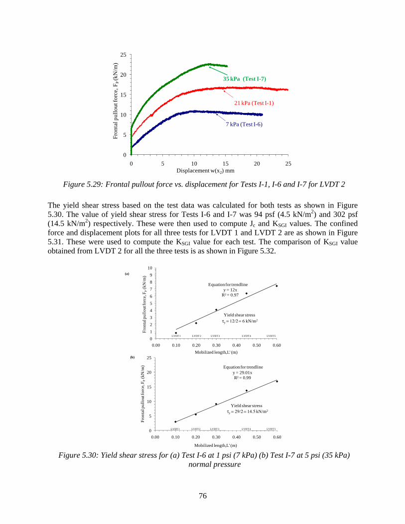
76

Figure 5.29: Frontal pullout force vs. displacement for Tests I-1, I-6 and I-7 for LVDT 2

The yield shear stress based on the test data was calculated for both tests as shown in Figure 5.30. The value of yield shear stress for Tests I-6 and I-7 was 94 psf (4.5 kN/m2) and 302 psf (14.5 kN/m2) respectively. These were then used to compute Jc and KSGI values. The confined force and displacement plots for all three tests for LVDT 1 and LVDT 2 are as shown in Figure 5.31. These were used to compute the KSGI value for each test. The comparison of KSGI value obtained from LVDT 2 for all the three tests is as shown in Figure 5.32.

Figure 5.30: Yield shear stress for (a) Test I-6 at 1 psi (7 kPa) (b) Test I-7 at 5 psi (35 kPa)

normal pressure

0

5

10

15

20

25

0 5 10 15 20 25

Fro

ntal

pul

lout

forc

e, F

P (k

N/m

)

Displacement w(x2) mm

21 kPa (Test I-1)

7 kPa (Test I-6)

35 kPa (Test I-7)

y = 12xR² = 0.97

0

1

2

3

4

5

6

7

8

9

10

0.00 0.10 0.20 0.30 0.40 0.50 0.60

Fron

tal p

ullo

ut fo

rce,

FP

(kN

/m)

Mobilized length,L' (m)

LVDT 1 LVDT 4LVDT 3LVDT 2 LVDT 5

Equation for trendline

Yield shear stressτy = 12/2 = 6 kN/m2

y = 29.01xR² = 0.99

0

5

10

15

20

25

0.00 0.10 0.20 0.30 0.40 0.50 0.60

Fron

tal p

ullo

ut fo

rce,

FP

(kN

/m)

Mobilized length,L' (m)

LVDT 1 LVDT 4LVDT 3LVDT 2 LVDT 5

τy = 29/2 = 14.5 kN/m2

Equation for trendline

Yield shear stress

(a)

(b)

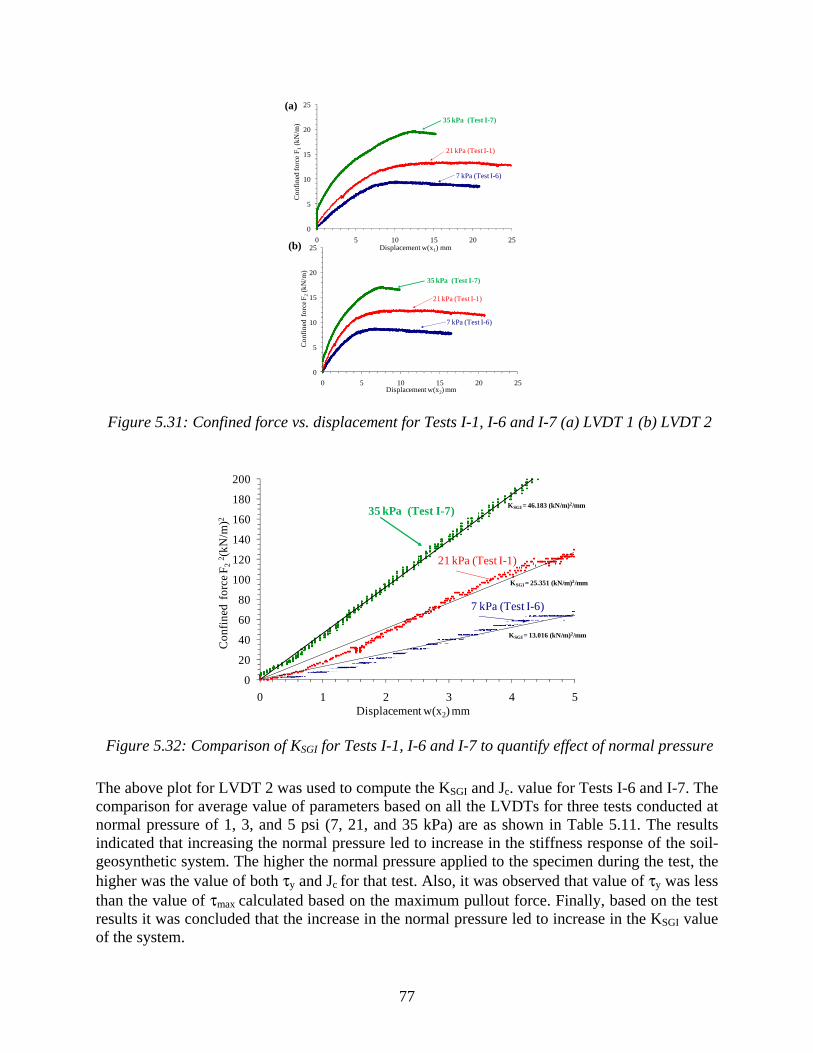
77

Figure 5.31: Confined force vs. displacement for Tests I-1, I-6 and I-7 (a) LVDT 1 (b) LVDT 2

Figure 5.32: Comparison of KSGI for Tests I-1, I-6 and I-7 to quantify effect of normal pressure

The above plot for LVDT 2 was used to compute the KSGI and Jc. value for Tests I-6 and I-7. The comparison for average value of parameters based on all the LVDTs for three tests conducted at normal pressure of 1, 3, and 5 psi (7, 21, and 35 kPa) are as shown in Table 5.11. The results indicated that increasing the normal pressure led to increase in the stiffness response of the soil-geosynthetic system. The higher the normal pressure applied to the specimen during the test, the higher was the value of both τy and Jc for that test. Also, it was observed that value of τy was less than the value of τmax calculated based on the maximum pullout force. Finally, based on the test results it was concluded that the increase in the normal pressure led to increase in the KSGI value of the system.

0

5

10

15

20

25

0 5 10 15 20 25

Con

fine

d fo

rce

F1

(kN

/m)

Displacement w(x1) mm

21 kPa (Test I-1)

7 kPa (Test I-6)

35 kPa (Test I-7)

0

5

10

15

20

25

0 5 10 15 20 25

Con

fine

d f

orce

F2

(kN

/m)

Displacement w(x2) mm

21 kPa (Test I-1)

7 kPa (Test I-6)

35 kPa (Test I-7)

(a)

(b)

0

20

40

60

80

100

120

140

160

180

200

0 1 2 3 4 5

Con

fine

d f

orce

F2

2 (kN

/m)2

Displacement w(x2) mm

21 kPa (Test I-1)

7 kPa (Test I-6)

35 kPa (Test I-7)KSGI = 46.183 (kN/m)2/mm

KSGI = 25.351 (kN/m)2/mm

KSGI = 13.016 (kN/m)2/mm

78

Table 5.11: Effect of normal pressure on KSGI

Effect of Orientation

The geosynthetic has two principal directions: longitudinal (or machine) and transverse (or cross-machine) direction. The testing direction of a geosynthetic in the pullout test is one in which force is applied, similar to conducting a tensile test on it. Therefore one pullout test was run to evaluate the interaction properties of change in orientation by pulling the specimen in the longitudinal (or machine) direction.

The test results were used to characterize and compare the properties of geosynthetic G3 with the baseline Test I-1. The effect of change in specimen direction was quantified by conducting a test similar to the baseline test, but reversing the principal directions of the specimen. The specimen was prepared for confined length of 0.6m and width of 0.45m and then subjected to a normal pressure of 3 psi (21 kPa). The frontal pullout force values corresponding to displacements for the five LVDT locations were obtained. The comparison for the frontal pullout force values obtained from LVDT 2 for Test I-1 and Test I-8 are shown in Figure 5.33a. The maximum pullout force value obtained in Test I-8 was 1.23 kip/ft (18 kN/m) as compared to value of 1 kip/ft (14.5 kN/m) obtained for Test I-1. Furthermore, the yield shear stress value was obtained for this tests based on LVDT movement was 1.09 kip/ft (16 kN/m as shown in Figure 5.33b. Finally, using the yield shear stress value, the KSGI value for the test was computed as shown in Figure 4.38c.

The average values of parameters obtained for both tests are shown in Table 5.12. The value of KSGI was lower in Test I-8 than in Test I-1 as the area of stronger longitudinal ribs was reduced when specimen was tested in machine direction.

Table 5.12: Effect of specimen direction on KSGI

Test Specimen dim. Normal pressure

Pullout parameters

Model parameters

Constant

L W NP Fmax τmax Jc τy KSGI MSGI,1mm

m m kPa kN/m kN/m2 kN/m kN/m2 (kN/m)2/m kN/m2 I-6 0.60 0.45 7 11.0 9.2 500 6.0 12000 3464 I-1 0.60 0.45 21 14.5 12.1 590 10.5 24780 4978 I-7 0.60 0.45 35 22.0 18.3 773 14.5 44834 6696

Test Specimen dim. Pullout

parameters Model

parameters Constant

L W Fmax τmax Jc τy KSGI MSGI,1mm

m m kN/m kN/m2 kN/m kN/m2 (kN/m)2/m kN/m2 I-1 0.60 0.45 14.5 12.1 590 10.5 24780 4978 I-8 0.60 0.45 18.5 15.4 220 16.0 14500 3808

79

Figure 5.33: Comparison of tests (I-1 and I-8) conducted to evaluate effect of specimen direction on parameters: (a) Maximum pullout force (b) Yield shear stress (c) KSGI

0.0

2.5

5.0

7.5

10.0

12.5

15.0

17.5

20.0

0 1 2 3 4 5 6 7 8 9 10 11 12 13 14 15 16 17 18 19 20 21 22 23 24 25

Fro

ntal

pul

lout

for

ce, F

p (k

N/m

)

Displacement, w(x2), mm

Test I-1(XD)

Test I-8(MD)

0.0

2.5

5.0

7.5

10.0

12.5

15.0

17.5

20.0

0.00 0.05 0.10 0.15 0.20 0.25 0.30 0.35 0.40 0.45 0.50 0.55 0.60

Fro

ntal

pul

lout

for

ce, F

p (k

N/m

)

Mobilized length, L' (m)

τy = 21/2= 10.5 kN/m2

Test I-1 (XD)

Test I-8 (MD)τy = 32/2 = 16 kN/m2

0

10

20

30

40

50

0.0 0.5 1.0 1.5 2.0 2.5

Con

fine

d fo

rce

, F(x

2)2 ,

(k

N/m

)2

Displacement, w(x2), mm

Test I-8 (MD)

Test I-1(XD)

(a)

(b)

(c)

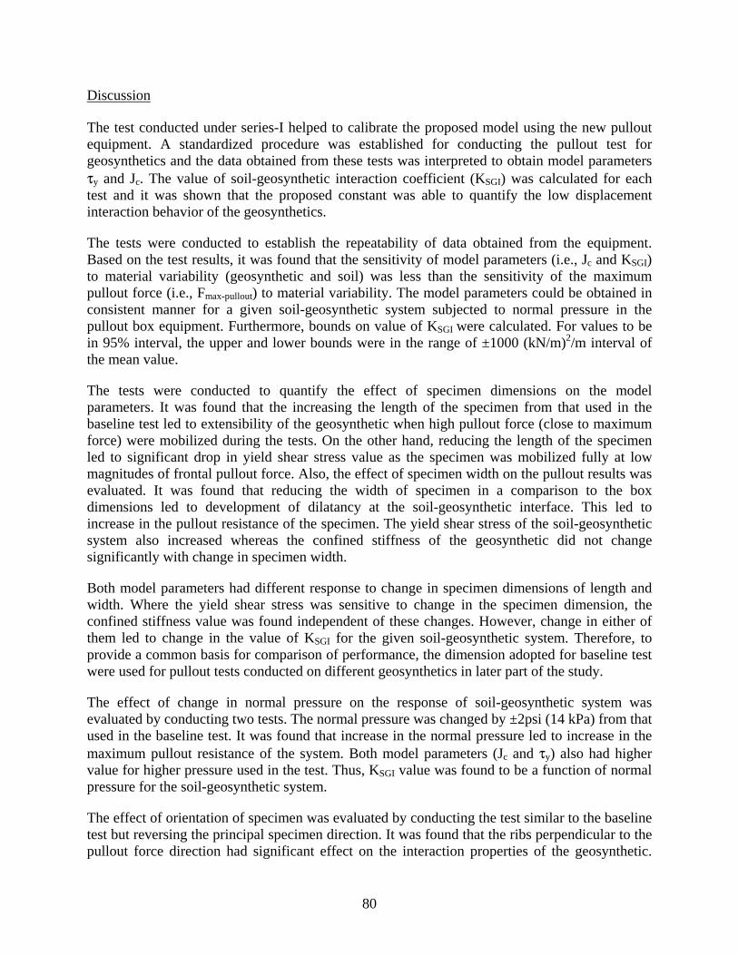
80

Discussion

The test conducted under series-I helped to calibrate the proposed model using the new pullout equipment. A standardized procedure was established for conducting the pullout test for geosynthetics and the data obtained from these tests was interpreted to obtain model parameters τy and Jc. The value of soil-geosynthetic interaction coefficient (KSGI) was calculated for each test and it was shown that the proposed constant was able to quantify the low displacement interaction behavior of the geosynthetics.

The tests were conducted to establish the repeatability of data obtained from the equipment. Based on the test results, it was found that the sensitivity of model parameters (i.e., Jc and KSGI) to material variability (geosynthetic and soil) was less than the sensitivity of the maximum pullout force (i.e., Fmax-pullout) to material variability. The model parameters could be obtained in consistent manner for a given soil-geosynthetic system subjected to normal pressure in the pullout box equipment. Furthermore, bounds on value of KSGI were calculated. For values to be in 95% interval, the upper and lower bounds were in the range of ±1000 (kN/m)2/m interval of the mean value.

The tests were conducted to quantify the effect of specimen dimensions on the model parameters. It was found that the increasing the length of the specimen from that used in the baseline test led to extensibility of the geosynthetic when high pullout force (close to maximum force) were mobilized during the tests. On the other hand, reducing the length of the specimen led to significant drop in yield shear stress value as the specimen was mobilized fully at low magnitudes of frontal pullout force. Also, the effect of specimen width on the pullout results was evaluated. It was found that reducing the width of specimen in a comparison to the box dimensions led to development of dilatancy at the soil-geosynthetic interface. This led to increase in the pullout resistance of the specimen. The yield shear stress of the soil-geosynthetic system also increased whereas the confined stiffness of the geosynthetic did not change significantly with change in specimen width.

Both model parameters had different response to change in specimen dimensions of length and width. Where the yield shear stress was sensitive to change in the specimen dimension, the confined stiffness value was found independent of these changes. However, change in either of them led to change in the value of KSGI for the given soil-geosynthetic system. Therefore, to provide a common basis for comparison of performance, the dimension adopted for baseline test were used for pullout tests conducted on different geosynthetics in later part of the study.

The effect of change in normal pressure on the response of soil-geosynthetic system was evaluated by conducting two tests. The normal pressure was changed by ±2psi (14 kPa) from that used in the baseline test. It was found that increase in the normal pressure led to increase in the maximum pullout resistance of the system. Both model parameters (Jc and τy) also had higher value for higher pressure used in the test. Thus, KSGI value was found to be a function of normal pressure for the soil-geosynthetic system.

The effect of orientation of specimen was evaluated by conducting the test similar to the baseline test but reversing the principal specimen direction. It was found that the ribs perpendicular to the pullout force direction had significant effect on the interaction properties of the geosynthetic.

81

The value of model parameters for the same normal pressure was different in both tests. For pavement application, loading conditions are multi-dimensional in nature. The tires travel direction is parallel to the machine direction of the geosynthetic when a vehicle is driven over a roadway. This leads to localized shear forces in the cross-machine ribs of the geosynthetic causing mobilization of lateral restraint mechanism in the system. The cross-machine direction response is considered critical for geosynthetic reinforced pavement application. However, tests were done in both machine and cross-machine direction for geosynthetics tested in the study as it was found that the combined response and interaction between junctions of geogrids would govern the final performance of the reinforced pavement system. The results of tests conducted on geogrids are discussed in the next section, Series II: Large Pullout Tests for Comparison between Two Geogrids of Same Material.

Eight tests were conducted in this series of pullout testing was as shown in Table 2.1. Each test was setup similar to the Test I-1 in terms of specimen dimensions—2 ft (0.6 m) confined length and 1.5 ft (0.45 m) width—LVDT locations, i.e., 4 in. (100 mm), 8 in. (200 mm), 12 in. (300 mm), 18 in. (450 mm), and 24 in. (600 mm) from the front end of the specimen, and the soil used (Monterey No.30 sand). Each geosynthetic was tested in the cross-machine direction at three normal pressures of 1, 3, and 5 psi (7, 21, and 35 kPa) and in machine direction at normal pressure of 1 psi (21 kPa). The comparison of results obtained for both geogrids at each applied normal pressure magnitude are discussed in the next section.

Series II: Large Pullout Tests for Comparison between Two Geogrids of Same Material

Tests II-1, II-2, and II-3 were conducted on geogrid G1 and II-4, II-5, and II-6 were conducted on geogrid G4 in cross-machine direction at normal pressures of 1, 3, and 5 psi (7, 21, and 35 kPa) on the top of the specimen as was listed in Table 2.1. The frontal pullout forces vs. displacement curve for each test are as shown in Figure 5.34. Based on the results, it was observed that at each normal pressure level the value of maximum pullout force obtained for geogrid G4 was greater than that for geogrid G1.

The model parameters τy and Jc were calculated based on these tests. The comparison of yield shear stress value obtained at given normal pressure for both geogrids is shown in Figure 5.35. It was observed that the geogrid G4 had higher yield shear stress than G1 at each normal pressure. This is primarily attributed to the higher thickness of ribs in G4 than G1. This led to better shear stress development at its surface during the pullout test when compared with geogrid G1.

82

Figure 5.34: Frontal pullout force vs. displacement for G1 and G4: (a) 1 psi (7kPa); (b) 3 psi (21kPa); (c) 5 psi (35 kPa)

0.0

2.5

5.0

7.5

10.0

12.5

15.0

17.5

20.0

0 1 2 3 4 5 6 7 8 9 10 11 12 13 14 15 16 17 18 19 20

Fro

ntal

pul

lout

for

ce, F

p (k

N/m

)

Displacement, w(x1), mm

7 kPa

Test II-1 (G1)

Test II-4 (G4)

0.0

2.5

5.0

7.5

10.0

12.5

15.0

17.5

20.0

0 1 2 3 4 5 6 7 8 9 10 11 12 13 14 15 16 17 18 19 20

Fro

ntal

pul

lout

for

ce, F

p (k

N/m

)

Displacment, w(x1),mm

21 kPa

Test II-2 (G1)

Test II-5 (G4)

0.0

2.5

5.0

7.5

10.0

12.5

15.0

17.5

20.0

0 1 2 3 4 5 6 7 8 9 10 11 12 13 14 15 16 17 18 19 20

Fro

ntal

pul

lout

for

ce, F

p (k

N/m

)

Displacment, w(x1),mm

35 kPa

Test II-3 (G1)

Test II-6 (G4)

(a)

(b)

(c)

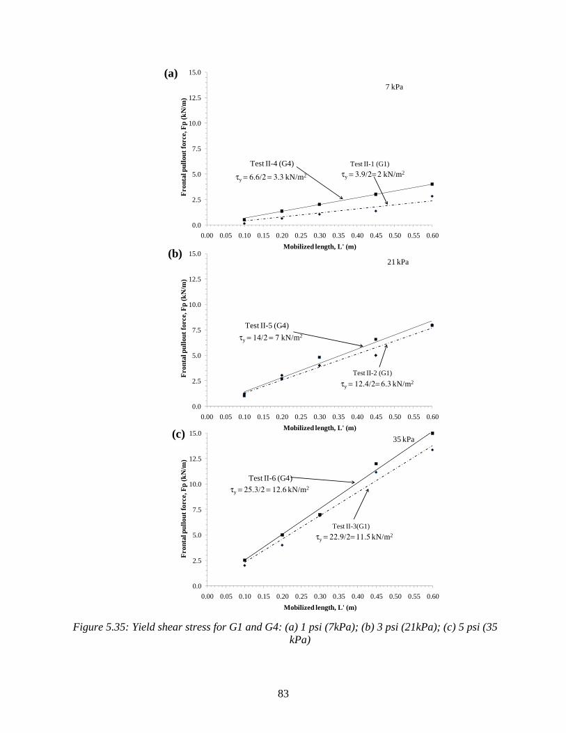
83

Figure 5.35: Yield shear stress for G1 and G4: (a) 1 psi (7kPa); (b) 3 psi (21kPa); (c) 5 psi (35 kPa)

0.0

2.5

5.0

7.5

10.0

12.5

15.0

0.00 0.05 0.10 0.15 0.20 0.25 0.30 0.35 0.40 0.45 0.50 0.55 0.60

Fro

ntal

pul

lout

for

ce, F

p (k

N/m

)

Mobilized length, L' (m)

τy = 3.9/2= 2 kN/m2τy = 6.6/2 = 3.3 kN/m2

7 kPa

Test II-1 (G1)Test II-4 (G4)

0.0

2.5

5.0

7.5

10.0

12.5

15.0

0.00 0.05 0.10 0.15 0.20 0.25 0.30 0.35 0.40 0.45 0.50 0.55 0.60

Fro

ntal

pul

lout

for

ce, F

p (k

N/m

)

Mobilized length, L' (m)

τy = 12.4/2= 6.3 kN/m2

τy = 14/2 = 7 kN/m2

21 kPa

Test II-2 (G1)

Test II-5 (G4)

0.0

2.5

5.0

7.5

10.0

12.5

15.0

0.00 0.05 0.10 0.15 0.20 0.25 0.30 0.35 0.40 0.45 0.50 0.55 0.60

Fro

ntal

pul

lout

for

ce, F

p (k

N/m

)

Mobilized length, L' (m)

τy = 22.9/2= 11.5 kN/m2

τy = 25.3/2 = 12.6 kN/m2

35 kPa

Test II-3(G1)

Test II-6 (G4)

(a)

(b)

(c)

84

The test results were used to compute the KSGI value for each test by plotting the square of confined force value with displacement at LVDT 2. The comparison of KSGI value for each normal pressure level for two geogrids is shown in Figure 5.36. It was observed that G4 had higher KSGI value at each normal pressure level than G1. The difference in performance was greatest at low confining pressure, but the differences were less significant for higher normal pressure. For reinforced pavement, the performance under low normal stresses is the most important, so G4 was consider better suited than G1 for pavement reinforcement.

Figure 5.36: KSGI for G1 and G4: (a) 1 psi (7kPa); (b) 3 psi (21kPa); (c) 5 psi (35 kPa)

KSGI = 1.5013 (kN/m)2/mm

KSGI = 6.0079 (kN/m)2/mm

0

1

2

3

4

5

6

7

8

9

10

0.0 0.5 1.0 1.5 2.0 2.5

Con

fine

d fo

rce

, F(x

2)2 ,

(k

N/m

)2

Displacement, w(x2), mm

7 kPa

Test II-1 (G1)

Test II-4 (G4)

y = 14.974x

KSGI = 22.315(kN/m)2/mm

0

10

20

30

40

50

0.0 0.5 1.0 1.5 2.0 2.5

Con

fine

d fo

rce

, F(x

2)2 ,

(k

N/m

)2

Displacement, w(x2), mm

21 kPa

Test II-2 (G1)

Test II-5 (G4)

KSGI = 43.969 (kN/m)2/mm

KSGI= 34.306 (kN/m)2/mm

0

10

20

30

40

50

60

70

80

90

100

0.0 0.5 1.0 1.5 2.0 2.5

Con

fine

d fo

rce

, F(x

2)2 ,

(k

N/m

)2

Displacement, w(x2), mm

35 kPa

Test II-3 (G1)

Test II-6 (G4)

(a)

(b)

(c)

85

The values of Jc were back calculated for all the tests as shown in Table 5.13. Based on the results it was observed that an increase in normal pressure leads to increasing values of Jc for both geogrids. Furthermore, for each normal pressure, G4 showed higher Jc value than G1 indicating better performance under confined conditions. This trend was similar to that observed for unconfined tensile strength of these geogrids, where G4 had higher strength than G1 in the cross-machine direction.

Table 5.13: Effect of geogrid type on KSGI

Tests II-7 and II-8 were done on geogrid G1 and G4 in machine direction at normal pressure of 3 psi (21kPa) on the top of the specimen as was listed in Table 2.1. The frontal pullout forces vs. displacement curve for each test are as shown in Figure 5.37a. Furthermore, the yield shear stress value was computed for both geogrids as shown in Figure 5.37b. Finally, the results obtained were used to compute the KSGI value for each test as shown in Figure 5.37c. The values of Jc

were then back calculated for all the tests and are as shown in Table 5.14.

Table 5.14: Effect of geogrid testing orientation on KSGI

Test Abbreviation Specimen dim. Normal pressure

Pullout parameters

Model parameters

Constant

L W NP Fmax τmax Jc τy KSGI MSGI,1mm

m m kPa kN/m kN/m2 kN/m kN/m2 (kN/m)2/m kN/m2 II-1 G1-XD-7 0.60 0.45 7 5.0 4.2 188 2.0 1501 1225 II-2 G1-XD-21 0.60 0.45 21 12.2 10.2 594 6.3 14974 3870 II-3 G1-XD-35 0.60 0.45 35 15.5 12.9 745 11.5 34306 5857 II-4 G4-XD-7 0.60 0.45 7 7.5 6.3 500 3.0 6007 2451 II-5 G4-XD-21 0.60 0.45 21 12.7 10.5 796 7.0 22315 4723 II-6 G4-XD-35 0.60 0.45 35 17.5 16 872 12.6 43969 6630

Test Abbreviation Specimen dim. Normal pressure

Pullout parameters

Model parameters

Constant

L W NP Fmax τmax Jc τy KSGI MSGI,1mm

m m kPa kN/m kN/m2 kN/m kN/m2 (kN/m)2/m kN/m2 II-7 G1-MD-21 0.60 0.45 21 11.5 9.6 660 7.6 20145 4488 II-8 G4-MD-21 0.60 0.45 21 14 10.0 690 8.5 23500 4850

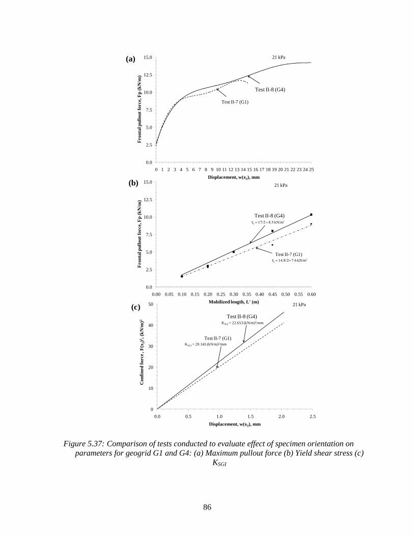
86

Figure 5.37: Comparison of tests conducted to evaluate effect of specimen orientation on parameters for geogrid G1 and G4: (a) Maximum pullout force (b) Yield shear stress (c)

KSGI

0.0

2.5

5.0

7.5

10.0

12.5

15.0

0 1 2 3 4 5 6 7 8 9 10 11 12 13 14 15 16 17 18 19 20 21 22 23 24 25

Fro

ntal

pul

lout

for

ce, F

p (k

N/m

)

Displacement, w(x2), mm

Test II-7 (G1)

Test II-8 (G4)

21 kPa

0.0

2.5

5.0

7.5

10.0

12.5

15.0

0.00 0.05 0.10 0.15 0.20 0.25 0.30 0.35 0.40 0.45 0.50 0.55 0.60

Fro

ntal

pul

lout

for

ce, F

p (k

N/m

)

Mobilized length, L' (m)

τy = 14.8/2= 7.6 kN/m2

Test II-7 (G1)

τy = 17/2 = 8.5 kN/m2

Test II-8 (G4)

21 kPa

KSGI = 20.145 (kN/m)2/mm

KSGI = 22.653 (kN/m)2/mm

0

10

20

30

40

50

0.0 0.5 1.0 1.5 2.0 2.5

Con

fine

d fo

rce

, F(x

2)2 ,

(k

N/m

)2

Displacement, w(x2), mm

Test II-7 (G1)

Test II-8 (G4)

21 kPa

(a)

(b)

(c)

87

Based on the results, it was observed that the geogrid G4 had slightly higher value for KSGI than geogrid G1 in the machine direction. The contrast in performance properties of both geogrids was not as significant as observed for tests in cross-machine direction. Because KSGI index involves properties of the soil, geosynthetic, and soil-geosynthetic interaction, it is inferred that the observed difference in KSGI value relates only to the physical properties of the geogrid specimens. Accordingly, KSGI trend was compared with physical properties of both geogrids. It was found that, similar to KSGI trends, both geogrids had similar properties in machine direction whereas different properties in cross-machine direction. Therefore, this experiment showed that KSGI can be considered as an index that effectively captures the effect of the geogrids on the confined interaction between soil and geosynthetic.

Discussion

The pullout tests conducted under series-II as explained in the section above helped to compare the properties of geogrids with similar physical properties but slightly different tensile strengths. The procedure established for pullout testing of geosynthetics as explained in test series-1 was adopted. The tests helped in establishing the applicability of SGI model to predict performance of geogrids.

The pullout test results where the unconfined properties of the geogrids were known were analyzed based on this model. The order of performance predicted based on the KSGI value was similar to that predicted by laboratory and field studies conducted on these geosynthetics earlier. The behavior predicted based on these tests showed good agreement with the physical characteristics of these products. Specifically, G4 consistently had higher coefficient value than G1 at the three confining pressure levels and in both directions of testing. Although the performance of geosynthetic reinforced pavements is expected to be affected by a number of factors, the higher KSGI value of G4 indicates that G4 performs better than G1 in reinforced pavement application. The reason is that higher KSGI value results in higher horizontal stiffness of reinforced pavement in confined condition, which leads to higher horizontal confinement of the base course layer. The higher horizontal confinement leads in turn to the lower lateral deformations and the better performance of the section.

A total of four tests were conducted in this series of pullout testing as shown in Table 2.1. Each test was setup similar to the Test I-1 in terms of specimen dimensions, i.e., 2 ft (0.6 m) confined length and 1.5 ft (0.45 m) width; LVDT locations, i.e., 4 in. (100 mm), 8 in. (200 mm), 12 in. (300 mm), 18 in. (450 mm), and 24 in. (600 mm) from the front end of the specimen; and the soil used—Monterey No.30 sand. The geosynthetic was tested in the cross-machine direction (III-1, III-2, and III-3) at three confining pressures of 1, 3, and 5 psi (7, 21, and 35 kPa) and in machine direction (III-4) at confining pressure of 3 psi (21 kPa). The results obtained for the geogrid at each confining pressure are discussed in the next section.

Series III: Large Pullout Tests on Geogrids of Different Materials

Tests III-1, III-2, and III-3 were conducted in cross-machine direction at normal pressure of 1, 3, and 5 psi (7, 21, and 35 kPa) on geogrid G2 as listed in Table 2.1. The frontal pullout forces vs. displacement curve for each test are as shown in Figure 5.38a. Furthermore, the yield shear stress value was computed at each normal pressure level for the geogrid as shown in Figure 5.38b.

88

Finally, the results obtained were used to compute the KSGI value for each test as shown in Figure 5.38c. The values of Jc back calculated for each test and are listed in Table 5.15. Based on the test results, it is observed that an increase in normal pressure leads to increasing value of these parameters.

89

Figure 5.38: Tests conducted to evaluate effect of confining pressure on parameters for geogrid G2 in cross machine direction: (a) Maximum pullout force (b) Yield shear stress (c) KSGI

0.0

2.5

5.0

7.5

10.0

12.5

15.0

17.5

20.0

0 1 2 3 4 5 6 7 8 9 10 11 12 13 14 15 16 17 18 19 20 21 22 23 24 25

Fro

ntal

pul

lout

for

ce, F

p (k

N/m

)

Displacement, w(x1), mm

Test III-1 (7 kPa)

Test III-2 (21 kPa)

Test III-3 (35 kPa)

y = 4.7x

y = 14.7x

y = 26.0x

0.0

2.5

5.0

7.5

10.0

12.5

15.0

0.00 0.05 0.10 0.15 0.20 0.25 0.30 0.35 0.40 0.45 0.50 0.55 0.60

Fro

ntal

pul

lout

for

ce, F

p (k

N/m

)

Mobilized length, L' (m)

τy = 4.7/2= 2.3 kN/m2

Test III-1 (7 kPa)

τy = 14.7/2 = 7.3 kN/m2

Test III-2 (21 kPa)τy = 26/2 = 13 kN/m2

Test III-3 (35 kPa)

KSGI = 1.271 (kN/m)2/mm

KSGI = 5.5027 (kN/m)2/mm

KSGI = 14.482 (kN/m)2/mm

0

1

2

3

4

5

6

7

8

9

10

0.0 0.5 1.0 1.5 2.0 2.5

Con

fine

d fo

rce

, F(x

2)2 ,

(k

N/m

)2

Displacement, w(x2), mm

Test III-1 (7 kPa)

Test III-2 (21 kPa)

Test III-3 (35 kPa)

(a)

(b)

(c)

90

Test III-4 was conducted in machine direction at normal pressure of 3 psi (21 kPa) using geogrid G2. The test helped to quantify the effect of change in specimen direction on model parameters. This test was conducted in similar manner as Test III-2, but by reversing the principal directions of the specimen. The frontal pullout force values corresponding to displacements for the five LVDT locations were obtained. The test results were analyzed to obtain the parameters as described in SGI model and is listed in Table 5.15.

Table 5.15: Results for geosynthetic G2 testing

The comparison of results for Tests III-2 and III-4 are shown in Figure 5.39. The frontal pullout force obtained from LVDT 2 for Test III-2 and Test III-4 is shown in Figure 5.39a. The geogrid (G3) shows higher pullout resistance in machine direction than cross-machine direction. The average yield shear stress value calculated based on initial displacement of five LVDTs for both tests is shown in Figure 5.39b. The specimen has twice the yield shear stress in cross-direction when compared with machine direction for same applied normal pressure. This was attributed to manufacturing of the geogrid, where the longitudinal ribs are thicker when compared to transverse ribs.

The comparison between KSGI values for both tests was conducted and is shown in Figure 5.39c. Based on the results shown in this figure, Jc values for both tests were back calculated as shown in Table 5.15. It was observed that the specimen had similar Jc values in both directions. This was similar to the unconfined tensile strength characteristics of this geosynthetics where it had same strength in both directions.

Test Abbreviation Specimen dim. Normal pressure

Pullout parameters

Model parameters

Constant

L W NP Fmax τmax Jc τy KSGI MSGI,1mm

m m kPa kN/m kN/m2 kN/m kN/m2 (kN/m)2/m kN/m2 III-1 G2-XD-7 0.60 0.45 7 5.1 4.3 159 2 1271 1127 III-2 G2-XD-21 0.60 0.45 21 12.0 10.0 189 7.3 5502 2345 III-3 G2-XD-35 0.60 0.45 35 15.5 12.9 279 13 14482 3805 III-4 G2-MD-7 0.60 0.45 7 17 14 185 14.5 10751 3275

91

Figure 5.39: Comparison of tests conducted to evaluate effect of specimen direction on

parameters for geogrid G2: (a) Maximum pullout force (b) Yield shear stress (c) KSGI

0.0

2.5

5.0

7.5

10.0

12.5

15.0

17.5

20.0

0 1 2 3 4 5 6 7 8 9 10 11 12 13 14 15 16 17 18 19 20 21 22 23 24 25

Fro

ntal

pul

lout

for

ce, F

p (k

N/m

)

Displacement, w(x1), mm

Test III-2 (XD)

Test III-4 (MD)

0.0

2.5

5.0

7.5

10.0

12.5

15.0

17.5

20.0

0.00 0.05 0.10 0.15 0.20 0.25 0.30 0.35 0.40 0.45 0.50 0.55 0.60

Fro

ntal

pul

lout

for

ce, F

p (k

N/m

)

Mobilized length, L' (m)

τy = 14.7/2 = 7.3 kN/m2

Test III-2 (XD)

τy = 29/2 = 14.5 kN/m2

Test III-4 (MD)

KSGI = 10.751 (kN/m)2/mm

KSGI = 5.5027 (kN/m)2/mm

0

2

4

6

8

10

12

14

16

18

20

0.0 0.5 1.0 1.5 2.0 2.5

Con

fine

d fo

rce

, F(x

2)2 ,

(k

N/m

)2

Displacement, w(x2), mm

Test III-2 (XD)

Test III-4 (MD)

(a)

(b)

(c)

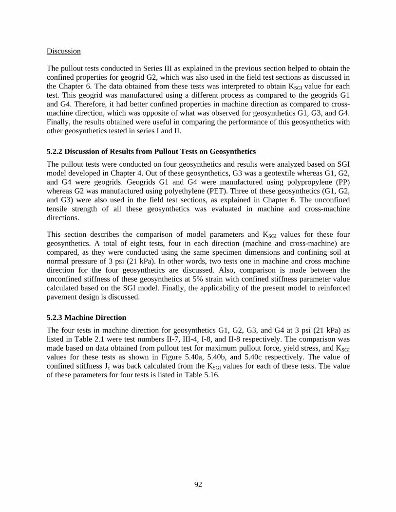
92

Discussion

The pullout tests conducted in Series III as explained in the previous section helped to obtain the confined properties for geogrid G2, which was also used in the field test sections as discussed in the Chapter 6. The data obtained from these tests was interpreted to obtain KSGI value for each test. This geogrid was manufactured using a different process as compared to the geogrids G1 and G4. Therefore, it had better confined properties in machine direction as compared to cross-machine direction, which was opposite of what was observed for geosynthetics G1, G3, and G4. Finally, the results obtained were useful in comparing the performance of this geosynthetics with other geosynthetics tested in series I and II.

5.2.2 Discussion of Results from Pullout Tests on Geosynthetics

The pullout tests were conducted on four geosynthetics and results were analyzed based on SGI model developed in Chapter 4. Out of these geosynthetics, G3 was a geotextile whereas G1, G2, and G4 were geogrids. Geogrids G1 and G4 were manufactured using polypropylene (PP) whereas G2 was manufactured using polyethylene (PET). Three of these geosynthetics (G1, G2, and G3) were also used in the field test sections, as explained in Chapter 6. The unconfined tensile strength of all these geosynthetics was evaluated in machine and cross-machine directions.

This section describes the comparison of model parameters and KSGI values for these four geosynthetics. A total of eight tests, four in each direction (machine and cross-machine) are compared, as they were conducted using the same specimen dimensions and confining soil at normal pressure of 3 psi (21 kPa). In other words, two tests one in machine and cross machine direction for the four geosynthetics are discussed. Also, comparison is made between the unconfined stiffness of these geosynthetics at 5% strain with confined stiffness parameter value calculated based on the SGI model. Finally, the applicability of the present model to reinforced pavement design is discussed.

5.2.3 Machine Direction

The four tests in machine direction for geosynthetics G1, G2, G3, and G4 at 3 psi (21 kPa) as listed in Table 2.1 were test numbers II-7, III-4, I-8, and II-8 respectively. The comparison was made based on data obtained from pullout test for maximum pullout force, yield stress, and KSGI values for these tests as shown in Figure 5.40a, 5.40b, and 5.40c respectively. The value of confined stiffness Jc was back calculated from the KSGI values for each of these tests. The value of these parameters for four tests is listed in Table 5.16.

93

Figure 5.40: Comparison of tests conducted in machine direction for geosynthetics G1, G2, G3

and G4: (a) Maximum pullout force (b) Yield shear stress (c) KSGI

0.0

2.5

5.0

7.5

10.0

12.5

15.0

17.5

20.0

0 1 2 3 4 5 6 7 8 9 10 11 12 13 14 15

Fro

ntal

pul

lout

for

ce, F

p (k

N/m

)

Displacement, w(x2), mm

Test II-7 (G1)

Test II-8 (G4)

Test III-4 (G2)

Test I-8 (G3)

0.0

2.5

5.0

7.5

10.0

12.5

15.0

17.5

20.0

0.00 0.05 0.10 0.15 0.20 0.25 0.30 0.35 0.40 0.45 0.50 0.55 0.60

Fro

ntal

pul

lout

for

ce, F

p (k

N/m

)

Mobilized length, L' (m)

τy = 7.6 kN/m2Test II-7 (G1)

τy = 8.5 kN/m2

Test II-8 (G4)

τy =14.5 kN/m2

Test III-4 (G2)

Test I-8 (G3)τy = 16 kN/m2

KSGI = 20.145(kN/m)2/mm

KSGI = 22.653 (kN/m)2/mm

KSGI = 14.119 (kN/m)2/mm

KSGI = 10.751 (kN/m)2/mm

0

10

20

30

40

50

0.0 0.5 1.0 1.5 2.0 2.5

Con

fine

d fo

rce

, F(x

2)2 ,

(k

N/m

)2

Displacement, w(x2), mm

Test II-7 (G1)

Test II-8 (G4)

Test III-4 (G2)

Test I-8 (G3)

(a)

(b)

(c)

94

Table 5.16: Comparison of KSGI for geosynthetics in machine direction

Based on the results it was concluded that the geosynthetic G3 had the maximum pullout resistance (see Fmax in Table 5.10) followed by geosynthetic G2, G4 and then G1 in decreasing order. However, the focus of the present implementation project is to characterize the interaction behavior under low displacement of soil-geosynthetic systems. Therefore, KSGI values of these geosynthetics were compared and it was found that G4 had highest value of all the geosynthetics followed by G1, G3, and then G2. The difference in KSGI values for these geosynthetics can be explained by examining the model parameter (τy and Jc) values for these geosynthetics. It was observed that products G1 and G4 (geosynthetics with same material) had higher confined stiffness Jc and lower yield shear stress τy when compared to G2 and G3 (geosynthetics from another manufacturer) for similar testing conditions. The geotextile G3 showed the highest value of yield shear stress when compared to other three geosynthetics (geogrids). Therefore, G3 would be product of choice if only the shear stress of the system was of concern as is the case for tensioned membrane effect in unpaved roads, which is mobilized at high displacement magnitudes. The flexible (paved) pavements require that the geosynthetic be mobilized under low displacements, as lateral restraint is the governing mechanism. Thus, not only shear stress but also confined stiffness of the geosynthetics is important. Therefore, geosynthetic G4 (which had the highest value of KSGI) was considered the best suited geosynthetic, among those tested in this study, for this application.

In summary, the proposed model allowed the dissimilar properties of these geosynthetics to be combined into a single framework and used for comparing their performance at low displacements using the KSGI value.

5.2.4 Cross-Machine Direction

The four tests in cross-machine direction for geosynthetics G1, G2, G3, and G4 at 3 psi (21 kPa) as listed in Table 2.1 were test numbers II-2, III-2, I-1, and II-5 respectively. The comparison was made based on data obtained from pullout test for maximum pullout force, yield stress, and KSGI values for these tests as shown in Figure 5.41a, 5.41b, and 5.41c respectively. The value of these parameters for four tests is listed in Table 5.17.

Test Abbreviation Specimen dim. Normal pressure

Pullout parameters

Model parameters

Constant

L W NP Fmax τmax Jc τy KSGI MSGI,1mm

m m kPa kN/m kN/m2 kN/m kN/m2 (kN/m)2/m kN/m2 II-7 G1-MD-21 0.60 0.45 21 11.5 9.6 660 7.6 20145 4488 III-4 G2-MD-21 0.60 0.45 21 17 14 185 14.5 10751 3275 I-8 G3-MD-21 0.60 0.45 21 18.5 15.4 220 16.0 14500 3808 II-8 G4-MD-21 0.60 0.45 21 14 10.0 690 8.5 23500 4850

95

Table 5.17: Comparison of KSGI for geosynthetics in cross-machine direction

Based on the results it may be concluded that the geosynthetic G3 (geotextile) has the maximum pullout resistance and yield shear stress values in cross-machine direction as compared to the other geosynthetics (geogrid). This trend is similar to that observed in machine direction for these geosynthetics. The yield shear stress value for three geogrids was in the range of 125 to 155 psf (6 to 7.5 kN/m2). Therefore, their performance could be distinguished by comparing the confined stiffness directly. Based on this parameter it is observed that geogrid G4 performed better than G1 followed by G2.

When KSGI values for all the four geosynthetics was compared, similar trend in performance was observed for three geogrids (G4>G1>G2) as in the machine direction. However, in cross-machine direction the geotextile G3 had the highest KSGI value. This may be attributed to stronger cross-machine direction fibers than machine direction fibers for this geosynthetic. When the confined stiffness value of G3 was compared with geogrids, its value was lower than that obtained for G4, equal for G1, and higher for G2 in this case.

Test Abbreviation Specimen dim. Normal pressure

Pullout parameters

Model parameters

Constant

L W NP Fmax τmax Jc τy KSGI MSGI,1mm

m m kPa kN/m kN/m2 kN/m kN/m2 (kN/m)2/m kN/m2 II-2 G1-XD-21 0.60 0.45 21 12.2 10.2 594 6.3 14974 3870 III-2 G2-XD-21 0.60 0.45 21 12.0 10.0 189 7.3 5502 2345 I-1 G3-XD-21 0.60 0.45 21 14.5 12.1 590 10.5 24780 4978 II-5 G4-XD-21 0.60 0.45 21 12.7 10.5 796 7.0 22315 4723

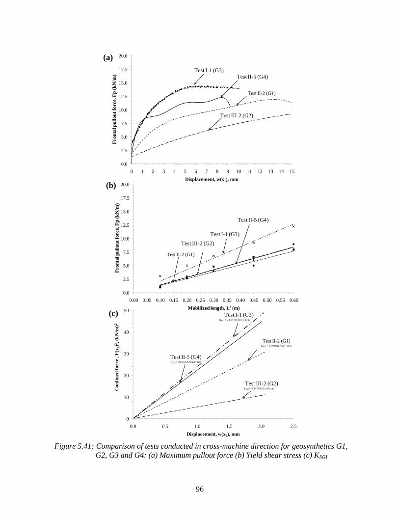
96

Figure 5.41: Comparison of tests conducted in cross-machine direction for geosynthetics G1,

G2, G3 and G4: (a) Maximum pullout force (b) Yield shear stress (c) KSGI

0.0

2.5

5.0

7.5

10.0

12.5

15.0

17.5

20.0

0 1 2 3 4 5 6 7 8 9 10 11 12 13 14 15

Fro

ntal

pul

lout

for

ce, F

p (k

N/m

)

Displacement, w(x1), mm

Test II-2 (G1)

Test II-5 (G4)

Test III-2 (G2)

Test I-1 (G3)

0.0

2.5

5.0

7.5

10.0

12.5

15.0

17.5

20.0

0.00 0.05 0.10 0.15 0.20 0.25 0.30 0.35 0.40 0.45 0.50 0.55 0.60

Fro

ntal

pul

lout

for

ce, F

p (k

N/m

)

Mobilized length, L' (m)

Test II-2 (G1)

Test II-5 (G4)

Test III-2 (G2)

Test I-1 (G3)

KSGI = 14.918 (kN/m)2/mm

KSGI = 22.653 (kN/m)2/mm

KSGI = 23.918 (kN/m)2/mm

KSGI = 5.3423(kN/m)2/mm

0

10

20

30

40

50

0.0 0.5 1.0 1.5 2.0 2.5

Con

fine

d fo

rce

, F(x

2)2 ,

(k

N/m

)2

Displacement, w(x2), mm

Test II-2 (G1)

Test II-5 (G4)

Test III-2 (G2)

Test I-1 (G3)

(a)

(b)

(c)

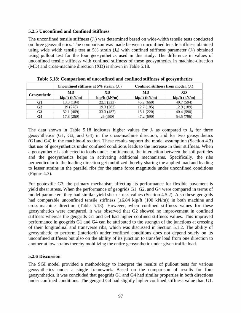
97

5.2.5 Unconfined and Confined Stiffness

The unconfined tensile stiffness (Ju) was determined based on wide-width tensile tests conducted on three geosynthetics. The comparison was made between unconfined tensile stiffness obtained using wide width tensile test at 5% strain (Ju) with confined stiffness parameter (Jc) obtained using pullout test for the four geosynthetics used in this study. The difference in values of unconfined tensile stiffness with confined stiffness of these geosynthetics in machine-direction (MD) and cross-machine direction (XD) is shown in Table 5.18.

Table 5.18: Comparison of unconfined and confined stiffness of geosynthetics

Unconfined stiffness at 5% strain, (Ju) Confined stiffness from model, (Jc)

Geosynthetic MD XD MD XD

kip/ft (kN/m) kip/ft (kN/m) kip/ft (kN/m) kip/ft (kN/m) G1 13.3 (194) 22.1 (323) 45.2 (660) 40.7 (594) G2 19 (278) 19.3 (282) 12.7 (185) 12.9 (189) G3 32.1 (469) 33.3 (487) 15.1 (220) 40.4 (590) G4 17.8 (260) 26 (380) 47.2 (690) 54.5 (796)

The data shown in Table 5.18 indicates higher values for Jc as compared to Ju for three geosynthetics (G1, G3, and G4) in the cross-machine direction, and for two geosynthetics (G1and G4) in the machine-direction. These results support the model assumption (Section 4.3) that use of geosynthetics under confined conditions leads to the increase in their stiffness. When a geosynthetic is subjected to loads under confinement, the interaction between the soil particles and the geosynthetics helps in activating additional mechanisms. Specifically, the ribs perpendicular to the loading direction get mobilized thereby sharing the applied load and leading to lesser strains in the parallel ribs for the same force magnitude under unconfined conditions (Figure 4.3).

For geotextile G3, the primary mechanism affecting its performance for flexible pavement is yield shear stress. When the performance of geogrids G1, G2, and G4 were compared in terms of model parameters they had similar yield shear stress values (Section 4.5.2). Also these geogrids had comparable unconfined tensile stiffness (±6.84 kip/ft (100 kN/m)) in both machine and cross-machine direction (Table 5.18). However, when confined stiffness values for these geosynthetics were compared, it was observed that G2 showed no improvement in confined stiffness whereas the geogrids G1 and G4 had higher confined stiffness values. This improved performance in geogrids G1 and G4 can be attributed to the strength of the junctions at crossing of their longitudinal and transverse ribs, which was discussed in Section 5.1.2. The ability of geosynthetic to perform (interlock) under confined conditions does not depend solely on its unconfined stiffness but also on the ability of its junction to transfer load from one direction to another at low strains thereby mobilizing the entire geosynthetic under given traffic load.

5.2.6 Discussion

The SGI model provided a methodology to interpret the results of pullout tests for various geosynthetics under a single framework. Based on the comparison of results for four geosynthetics, it was concluded that geogrids G1 and G4 had similar properties in both directions under confined conditions. The geogrid G4 had slightly higher confined stiffness value than G1.

98

When compared with geogrid G2, both geogrids G1 and G4 consistently showed better KSGI value in machine and cross machine direction. However, when results were compared with geotextile G3, it had contrasting properties in both directions. In machine direction it had lower value whereas in cross- machine direction it had higher value for KSGI than these geogrids.

The actual stress developed in pavement under wheel loading is biaxial in nature with larger strains in the transverse direction. Thus, it was assumed that a geosynthetic that can work as a combined unit would perform better under these circumstances rather than products with preferential direction of improved performance. Based on the analysis it was concluded that performance in descending order for the four geosynthetics would be G4 followed by G1, then G3 and finally G2. This performance order for geosynthetics was obtained for tests on Monterey No. 30 sand and thus is preliminary in nature. For actual pavement design, the geosynthetics are recommended to be tested in the project specific soil to determine the constant KSGI.

5.2.7 Conclusions

The suitability of the SGI model proposed in Chapter 4 for the analysis of the geosynthetic reinforced pavements was evaluated by conducting pullout tests. In the initial phase, pullout test equipment was designed with capability of measuring small displacement magnitudes at low normal pressures. A series of pullout tests were carried out using a geotextile and sand as baseline materials to calibrate the equipment. The consistency in the test results was established by running tests under similar conditions. The effect of model assumptions on the calculated constant was investigated by performing a parametric study of relevant variables. These studies included effect of specimen dimensions, normal pressure, and specimen direction on the parameter magnitude.

A good agreement was obtained between the first assumption of the proposed model and the experimental results. The linear relationship (with R2 > 0.95) between pullout force and mobilized length of geosynthetics, shown in the results of the tests, indicates an approximately constant value of τy in each test. This means that the interface shear stress has a uniform distribution throughout the geosynthetic specimen (as assumed in the first assumption of the model). In addition, repeatability of the experiments was shown in Tests I-1 and I-2 with observing a unique force-displacement relationship for a given pullout test. Moreover, the boundary conditions were found to affect the results from displacement LVDTs placed close to the specimen edges. Based on the results obtained a standardized procedure was established for the future testing.

The prediction of the performance was evaluated by comparing the pullout tests results of various geosynthetics. An extensive testing program was performed in order to evaluate the KSGI value for the geosynthetics in machine and cross machine direction at various confining pressures. The current state of practice involves evaluating the unconfined tensile strength of the geosynthetic and using it as a design input. Unlike current design assumptions, which typically assume that a higher unconfined tensile strength of the geosynthetic leads to better performance under confinement, this study showed that the geosynthetic capable of interlocking with soil and mobilizing its junctions and transverse ribs at low displacements would perform better in pullout tests (under confinement), independent of its unconfined tensile strength.

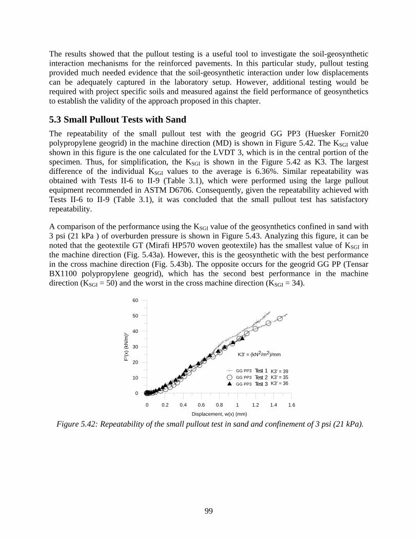
99

The results showed that the pullout testing is a useful tool to investigate the soil-geosynthetic interaction mechanisms for the reinforced pavements. In this particular study, pullout testing provided much needed evidence that the soil-geosynthetic interaction under low displacements can be adequately captured in the laboratory setup. However, additional testing would be required with project specific soils and measured against the field performance of geosynthetics to establish the validity of the approach proposed in this chapter.

5.3 Small Pullout Tests with Sand

The repeatability of the small pullout test with the geogrid GG PP3 (Huesker Fornit20 polypropylene geogrid) in the machine direction (MD) is shown in Figure 5.42. The KSGI value shown in this figure is the one calculated for the LVDT 3, which is in the central portion of the specimen. Thus, for simplification, the KSGI is shown in the Figure 5.42 as K3. The largest difference of the individual KSGI values to the average is 6.36%. Similar repeatability was obtained with Tests II-6 to II-9 (Table 3.1), which were performed using the large pullout equipment recommended in ASTM D6706. Consequently, given the repeatability achieved with Tests II-6 to II-9 (Table 3.1), it was concluded that the small pullout test has satisfactory repeatability.

A comparison of the performance using the KSGI value of the geosynthetics confined in sand with 3 psi (21 kPa ) of overburden pressure is shown in Figure 5.43. Analyzing this figure, it can be noted that the geotextile GT (Mirafi HP570 woven geotextile) has the smallest value of KSGI in the machine direction (Fig. 5.43a). However, this is the geosynthetic with the best performance in the cross machine direction (Fig. 5.43b). The opposite occurs for the geogrid GG PP (Tensar BX1100 polypropylene geogrid), which has the second best performance in the machine direction (KSGI = 50) and the worst in the cross machine direction (KSGI = 34).

Figure 5.42: Repeatability of the small pullout test in sand and confinement of 3 psi (21 kPa).

GG PP3 Test 1/19/2010

GG PP3 Test 1/20/2010

GG PP3 Test 1/21/2010

0

10

20

30

40

50

60

F2 (

x) (

kN/m

)2

0 0.2 0.4 0.6 0.8 1 1.2 1.4 1.6

Displacement, w(x) (mm)

Test 1Test 2Test 3

K3' = 39K3' = 35K3' = 36

K3' = (kN2/m2)/mm

100

(a) (b)

Figure 5.43: Comparison of the geosynthetics confined in sand and 3 psi. Specimen orientation: (a) machine direction and (b) cross machine direction.

5.4 Small Pullout Tests with Gravel

A comparison among the performance of the geosynthetics confined in gravel and 3 psi is shown in Figure 5.44. In this case, the GT has the worst performance in both orientations and the GG PP becomes the second worst in the machine direction (KSGI = 39, see Fig. 5.44a) and the best in the cross machine direction (KSGI = 95, Fig. 5.44b).

(a) (b)

Figure 5.44: Comparison among the geosynthetics in gravel and confinement of 3 psi. Specimen orientation: (a) machine direction and (b) cross machine direction.

This change in relative behavior of the geosynthetics when confined in sand and in gravel was not expected. It was expected that the magnitude of the values of the KSGI parameter would change when changing the soil from gravel to sand, but it was expected that the relative performance among the geosynthetics would remain the same. The Mont. No.30 sand was used in the testing program because is a standard soil and easy to handle, thus being an excellent candidate for a standard test. This difference in relative behavior of the geosynthetics when

GG PP

GG PET

GT

GG PP2

GG PP3

0

10

20

30

40

50

60

70

80F

2 (x)

(kN

/m)2

0 0.2 0.4 0.6 0.8 1 1.2 1.4 1.6 1.8 2

Displacement, w(x) (mm)

K3' = 50K3' = 56K3' = 29K3' = 54K3' = 39

K3' = (kN2/m2)/mm

GG PP

GG PET

GT

GG PP3

0

10

20

30

40

50

60

70

80

F2 (

x) (

kN/m

)2

0 0.2 0.4 0.6 0.8 1 1.2 1.4 1.6 1.8 2

Displacement, w(x) (mm)

K3' = 34K3' = 44K3' = 58K3' = 56

K3' = (kN2/m2)/mm

GG PP

GG PET

GTGG PP2

0

10

20

30

40

50

60

70

80

F2 (

x) (

kN/m

)2

0 0.2 0.4 0.6 0.8 1 1.2 1.4 1.6 1.8 2

Displacement, w(x) (mm)

K3' = 39K3' = 53K3' = 31K3' = 75

GG PP

GG PET

GTGG PP2

0

10

20

30

40

50

60

70

80

F2 (

x) (

kN/m

)2

0 0.2 0.4 0.6 0.8 1 1.2 1.4 1.6 1.8 2

Displacement, w(x) (mm)

K3' = 95K3' = 38K3' = 38K3' = 65

101

confined in sand and in gravel is due to the particle sizes and these particles interact with the reinforcement in different mechanisms.

Accordingly, some of the small pullout tests will be performed again for verification. Also, another convenient, standard soil that may have interaction mechanisms closer to the FM2 gravel will be used in additional small pullout tests.

102

103

Chapter 6. Field Monitoring Program

6.1 Field Test Section

The lessons learned from the field case studies formed the basis for a field monitoring program to evaluate the performance of geosynthetic reinforced pavements in Texas. As part of a highway maintenance and rehabilitation project, TxDOT supervised the construction of a geosynthetic reinforced farm-to-market road 2 (FM2), which was a low volume road in the Bryan District.

For comparative evaluation, the reinforced pavement was reconstructed using eight different reinforcement schemes (i.e., three reinforcement products and unreinforced control section, with/without lime stabilization). Furthermore to account for variation in field due to environmental, construction, and site factors, four repeats of each test section were constructed at the site. Therefore, a total of 32 test sections (4 reinforcement types x 2 stabilization approaches x 4 repeats) were constructed in FM2. Following are the significant features of the field monitoring program:

1. Test sections with different geosynthetic types, i.e., geogrid and geotextiles

2. Test sections with two different type of geogrids

3. Control sections with no geosynthetic to provide baseline for the study

4. Test sections having lime and no lime treatment

5. Multiple test sections with similar construction materials and geosynthetics

Due to the unique characteristics of this field study, the reinforced pavement was considered experimental and an extensive program of instrumentation for monitoring its post construction performance was implemented. In addition, instrumentation in the form of 32 moisture sensors was implemented in order to characterize the patterns of moisture migration under the pavement. A total of eight horizontal moisture and vertical moisture sensor profiles each containing an array of four sensors was installed below the pavement.

Field monitoring involving visual inspection, surveying, and falling weight deflectometer testing was conducted before reconstruction and immediately after reconstruction of the road. The final construction of the reinforced pavement was completed in January 2006 and performance evaluation of the newly reconstructed road was conducted on regular basis for the next three years. The results obtained from the field study provided understanding of the underlying fundamental mechanisms governing the performance of the geosynthetic reinforced pavement in field. Furthermore, they helped in quantify the mechanisms of longitudinal cracking and effectiveness of the geosynthetic reinforcements in mitigating such distresses.

6.2 Site Details

FM2 is located in Grimes County, which is in southeast part of Texas (Figure 6.1). The total length of the road is 6.4 miles, of which 2.4 miles lie towards the west of State Highway 6 (SH6) at Courtney; the other 4 miles continue eastward and end at FM362 (Figure 6.1b). The test sections were constructed in the portion of the road lying between SH6 and FM362. Details of

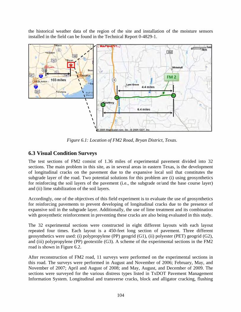
104

the historical weather data of the region of the site and installation of the moisture sensors installed in the field can be found in the Technical Report 0-4829-1.

Figure 6.1: Location of FM2 Road, Bryan District, Texas.

6.3 Visual Condition Surveys

The test sections of FM2 consist of 1.36 miles of experimental pavement divided into 32 sections. The main problem in this site, as in several areas in eastern Texas, is the development of longitudinal cracks on the pavement due to the expansive local soil that constitutes the subgrade layer of the road. Two potential solutions for this problem are (i) using geosynthetics for reinforcing the soil layers of the pavement (i.e., the subgrade or/and the base course layer) and (ii) lime stabilization of the soil layers.

Accordingly, one of the objectives of this field experiment is to evaluate the use of geosynthetics for reinforcing pavements to prevent developing of longitudinal cracks due to the presence of expansive soil in the subgrade layer. Additionally, the use of lime treatment and its combination with geosynthetic reinforcement in preventing these cracks are also being evaluated in this study.

The 32 experimental sections were constructed in eight different layouts with each layout repeated four times. Each layout is a 450-feet long section of pavement. Three different geosynthetics were used: (i) polypropylene (PP) geogrid (G1), (ii) polyester (PET) geogrid (G2), and (iii) polypropylene (PP) geotextile (G3). A scheme of the experimental sections in the FM2 road is shown in Figure 6.2.

After reconstruction of FM2 road, 11 surveys were performed on the experimental sections in this road. The surveys were performed in August and November of 2006; February, May, and November of 2007; April and August of 2008; and May, August, and December of 2009. The sections were surveyed for the various distress types listed in TxDOT Pavement Management Information System. Longitudinal and transverse cracks, block and alligator cracking, flushing

105

and raveling, patching, and rutting were measured during surveys. A 6-feet straight edge and a steel ruler were used for rutting measurements. From the first survey (May 2006) to the fifth survey (November 2007) no significant longitudinal cracks or marked distresses were observed.

However, surveys conducted from 2008 through December 2009 indicated various types of distresses including longitudinal cracking, rutting, potholes, weathering, and raveling. In general, the longitudinal cracks are developing in the shoulder and have started making their way towards the inside of the pavement. In this study, pavement is considered as just the portion of the traveled way of the road, for simplicity in reporting the results. The development of longitudinal cracks when rightly complemented with the precipitation data at the site shows that environmental loading, in the form of cycles of wetting and drying is taking place.

Although longitudinal cracks have developed in most of the test sections, no clear distinction can be established on the performance of the different geosynthetics in preventing this cracking. The cracks developed in the sections with reinforcement (with or without lime treatment) are outside the pavement, either near the outer end of the shoulder, in the shoulder or at the edge between shoulder and the traveled way of the road. Also, major distresses in the form of rutting, weathering and raveling, and longitudinal and transverse cracking are observed in the control sections (i.e., the sections with no reinforcement and no lime treatment) from the shoulder into the pavement. Moreover, the number of cracks developed in the control sections is consistently higher than the number of cracks developed in the other sections. Accordingly, a clear distinction between performances of the control and reinforced sections may be established given sufficient time for the cracks to evolve. With more cycles of wetting and drying as well as the traffic loading, the pavement structure and hence the layers are induced with stresses. A tensile stress must be induced in the reinforcement for its strength to be mobilized. Thus, over a period of 4 years and 11 condition surveys, an approximate differentiation in the performances of the 3 geosynthetics has been indicated.

In order to show the need for continuous monitoring of the evolution of the cracks in the test sections of the FM2 road, a summary of the cracks observed in the experimental sections is presented in this report. In this summary, pictures of the most important cracks in each section are shown to enhance the description of these features (Figures 6.3–6.26). General view pictures of the sections are provided for each section. In these pictures, it is possible to see the development of rutting in the sections.

The observed cracks are divided in three categories: (i) minor cracks, (ii) medium cracks, and (iii) major cracks. Minor cracks are cracks with a width not more than 0.2 in (5 mm). Major cracks are cracks with a width higher than 0.8 in (20 mm). Medium cracks are cracks with a width between 0.2 in and 0.8 in (5 mm and 20 mm).

106

Note: GG PP = Polypropylene (PP) Geogrid (GG). GG PET = Polyester (PET) Geogrid (GG). GT = Geotextile.

Figure 6.2: Experimental test sections at FM2 Road. (a) Section Profiles. (b) Location of sections.

(a)

(b)

107

6.3.1 Control Sections

Section #20 – 1Ea

Date of Survey Distresses Observed April 2008 1 minor longitudinal crack at outer edge of shoulder (Fig 6.3a). August 2008 4 major longitudinal cracks outside the road.

2 major longitudinal cracks in the shoulder. 1 longitudinal crack in the shoulder going into pavement (Fig. 6.3b). 2 cracks developing into pavement (Fig. 6.3c and Fig. 6.3d). 1 minor longitudinal crack inside pavement (Fig. 6.3e).

Figure 6.3: Distress observed in Control Section 1Ea (#20).

Dates:(a) April 2008; (b) to (e) August 2008

(b) (a)

(d)

(c)

(e)

108

Date of Survey Distresses Observed May 2009 1 crack developing into pavement (Fig. 6.4a).

1 crack developing into pavement from shoulder drop-off (Fig. 6.4b). Weathering and raveling (Fig. 6.4c).

June 2009 Major rutting and minor cracks (Fig 6.4d) in the paved area August 2009 Medium cracks propagate into the paved area (Fig 6.4e) December 2009 A patched pothole and tire marks- rutting (Fig 6.4f)

Figure 6.4: Distress observed in Control Section 1Ea (#20)

(b) (a) (c)

(d) (e) (f)

109

Section #1 – 1Wa

Date of Survey Distresses Observed April 2008 No cracks. August 2008 1 major longitudinal crack outside shoulder (Fig. 6.5a).

5 major longitudinal cracks in the shoulder (Fig. 6.5b). 1 double major crack outside shoulder (Fig. 6.5c).

May 2009 No cracks. High vegetation. General view (Fig. 6.5d).

August 2009 Deep rutting (Fig 6.5e) December 2009 Medium cracking in the paved area (Fig 6.5f)

Figure 6.5: Distress observed in Control Section 1Wa (#1).

Dates: (a) to (c) August 2008; (d) May 2009; (e) August 2009; (f) December 2009

(b) (a) (c)

(d) (e) (f)

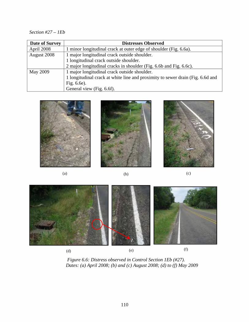
110

Section #27 – 1Eb

Date of Survey Distresses Observed April 2008 1 minor longitudinal crack at outer edge of shoulder (Fig. 6.6a). August 2008 1 major longitudinal crack outside shoulder.

1 longitudinal crack outside shoulder. 2 major longitudinal cracks in shoulder (Fig. 6.6b and Fig. 6.6c).

May 2009 1 major longitudinal crack outside shoulder. 1 longitudinal crack at white line and proximity to sewer drain (Fig. 6.6d and Fig. 6.6e). General view (Fig. 6.6f).

Figure 6.6: Distress observed in Control Section 1Eb (#27).

Dates: (a) April 2008; (b) and (c) August 2008; (d) to (f) May 2009

(b) (a) (c)

(d) (e) (f)

111

Date of Survey Distresses Observed June 2009 Medium cracking along the white line (Fig 6.7a) August 2009 Developed to major cracking (Fig 6.7b) December 2009 General picture indicating slope and topography (Fig 6.7c)

Figure 6.7: Distress observed in Control Section 1Eb. Dates: (a) June 2009; (b) August 2009; (c) December 2009

(b) (a)

(c)

112

Section #9 – 1Wb

Date of Survey Distresses Observed April 2008 No cracks. August 2008 2 longitudinal cracks in shoulder (Fig. 6.8a).

2 minor longitudinal cracks at outer shoulder edge. 1 major longitudinal crack outside shoulder.

May 2009 No cracks. June 2009 Shoulder drop off repair August 2009 Medium longitudinal cracking along shoulder

Figure 6.8: Distresses observed in Control Section 1Wb (#9).

Dates: (a) August 2008; (b) June 2009; (c) August 2009

(b) (a)

(c)

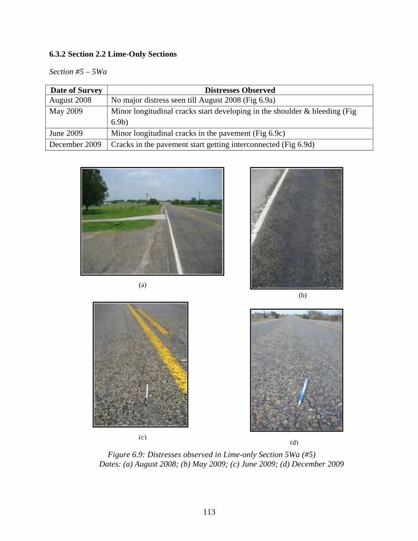
113

6.3.2 Section 2.2 Lime-Only Sections

Section #5 – 5Wa

Date of Survey Distresses Observed August 2008 No major distress seen till August 2008 (Fig 6.9a) May 2009 Minor longitudinal cracks start developing in the shoulder & bleeding (Fig

6.9b) June 2009 Minor longitudinal cracks in the pavement (Fig 6.9c) December 2009 Cracks in the pavement start getting interconnected (Fig 6.9d)

Figure 6.9: Distresses observed in Lime-only Section 5Wa (#5)

Dates: (a) August 2008; (b) May 2009; (c) June 2009; (d) December 2009

(b)

(a)

(c) (d)

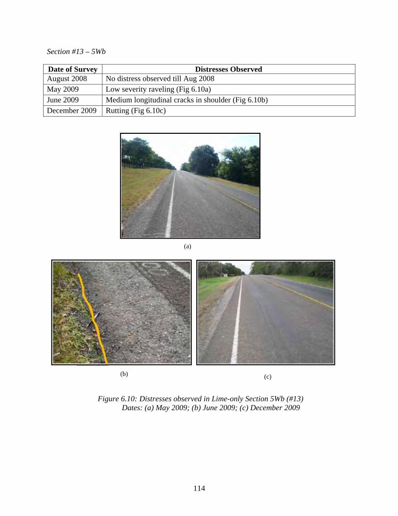
114

Section #13 – 5Wb

Date of Survey Distresses Observed August 2008 No distress observed till Aug 2008 May 2009 Low severity raveling (Fig 6.10a) June 2009 Medium longitudinal cracks in shoulder (Fig 6.10b) December 2009 Rutting (Fig 6.10c)

Figure 6.10: Distresses observed in Lime-only Section 5Wb (#13)

Dates: (a) May 2009; (b) June 2009; (c) December 2009

(b)

(a)

(c)

115

Section #24 – 5Ea

Date of Survey Distresses Observed August 2008 Minor longitudinal cracks in shoulder (Fig 6.11a) May 2009 Raveling (Fig 6.11b) June 2009 Major longitudinal cracking in the shoulder (Fig 6.11c) December 2009 Medium longitudinal cracks in the pavement (Fig 6.11d)

Figure 6.11: Distresses observed in Lime-only Section 5Ea (#24)

Dates: (a) August 2008; (b) May 2009; (c) June 2009; (d) December 2009

(b) (a)

(c) (d)

116

Section#31 – 5Eb

Date of Survey Distresses Observed August 2008 Huge shoulder drop-off (Fig 6.12a) May 2009 Rutting all through the section (Fig 6.12b) August 2009 Rutting, flushing, potholes, longitudinal and alligator cracking (Fig 6.12c) December 2009 Transverse and longitudinal cracks in the paved area (Fig 6.12d)

Figure 6.12: Distresses observed in Lime-only Section 5Eb (#31)

Dates: (a) August 2008; (b) May 2009; (c) June 2009; (d) December 2009

(b) (a)

(c) (d)

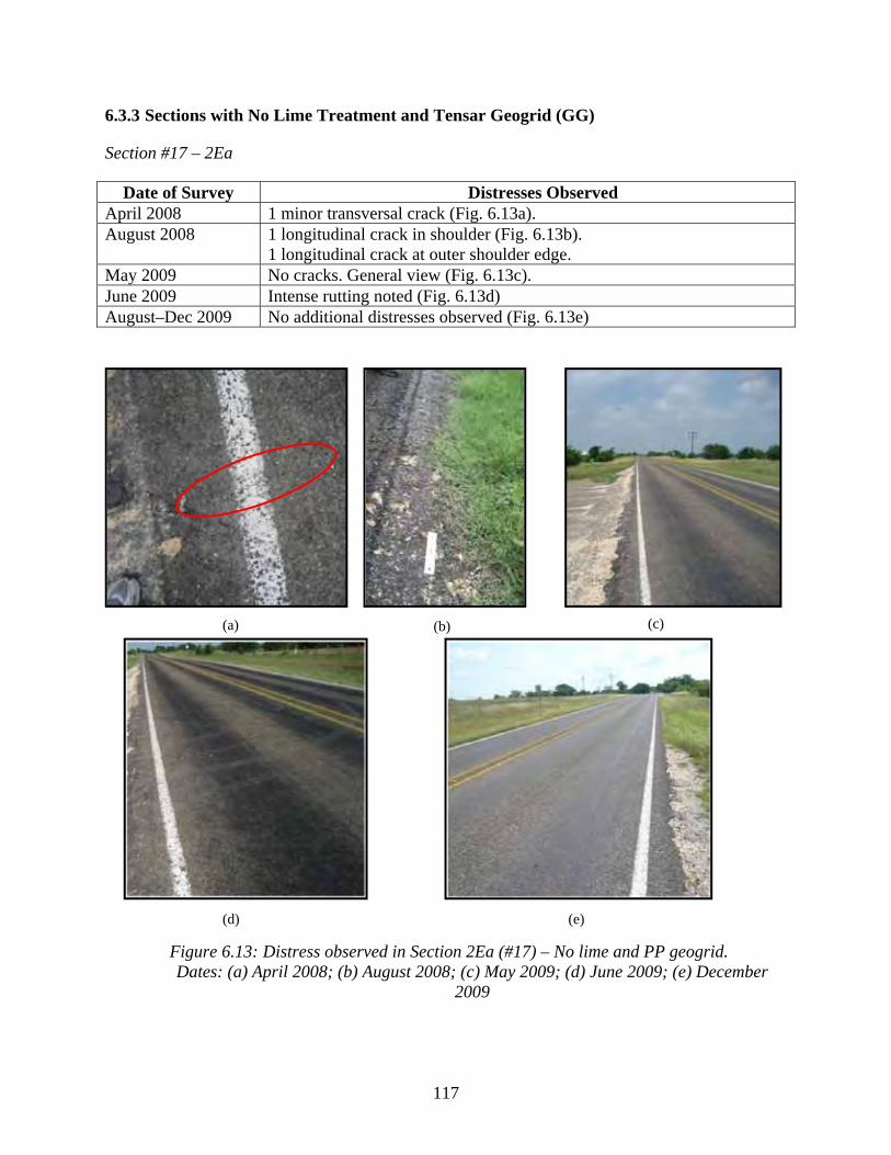
117

6.3.3 Sections with No Lime Treatment and Tensar Geogrid (GG)

Section #17 – 2Ea

Date of Survey Distresses Observed April 2008 1 minor transversal crack (Fig. 6.13a). August 2008 1 longitudinal crack in shoulder (Fig. 6.13b).

1 longitudinal crack at outer shoulder edge. May 2009 No cracks. General view (Fig. 6.13c). June 2009 Intense rutting noted (Fig. 6.13d) August–Dec 2009 No additional distresses observed (Fig. 6.13e)

Figure 6.13: Distress observed in Section 2Ea (#17) – No lime and PP geogrid. Dates: (a) April 2008; (b) August 2008; (c) May 2009; (d) June 2009; (e) December

2009

(b) (a) (c)

(d) (e)

118

Section #28 – 2Eb

Date of Survey Distresses Observed April 2008 No cracks. August 2008 1 longitudinal crack in shoulder (Fig. 6.14a).

1 longitudinal crack at outer shoulder edge. May 2009 No cracks. General view (Fig. 6.14b). June-August-December 2009

No additional distresses observed.

Figure 6.14: Cracks observed in Section 2Eb (#28) – No lime and PP geogrid.

Dates: (a) August 2008; (b) May 2009

(b) (a)

119

Section #2 – 2Wa

Date of Survey Distresses Observed April 2008 No cracks. August 2008 1 longitudinal crack at outer shoulder edge (Fig. 6.15a, 6.15b, and 6.15c).

Note that in Figure 6.15c the edge of the geogrid is right at where the longitudinal crack develops.

May 2009 1 longitudinal crack at outer shoulder edge (Fig. 6.15d). General view (Fig. 6.15e).

June-August- December 2009

No additional distresses observed at all.

Figure 6.15: Cracks observed in Section 2Wa (#2) – No lime and PP geogrid.

Dates: (a) to (c) August 2008; (d) and (e) May 2009

(b) (a) (c)

(d) (e)

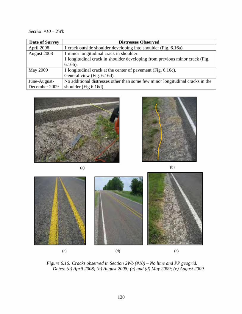
120

Section #10 – 2Wb

Date of Survey Distresses Observed April 2008 1 crack outside shoulder developing into shoulder (Fig. 6.16a). August 2008 1 minor longitudinal crack in shoulder.

1 longitudinal crack in shoulder developing from previous minor crack (Fig. 6.16b).

May 2009 1 longitudinal crack at the center of pavement (Fig. 6.16c). General view (Fig. 6.16d).

June-August-December 2009

No additional distresses other than some few minor longitudinal cracks in the shoulder (Fig 6.16d)

Figure 6.16: Cracks observed in Section 2Wb (#10) – No lime and PP geogrid.

Dates: (a) April 2008; (b) August 2008; (c) and (d) May 2009; (e) August 2009

(b) (a)

(c) (d) (e)

121

6.3.4 Sections with No Lime Treatment and Mirafi (PET) Geogrid (GG).

Section #18 – 3Ea

Date of Survey Distresses Observed April 2008 No cracks. August 2008 2 longitudinal cracks outside shoulder (Fig. 6. 17a). May 2009 No cracks. High vegetation. June 2009 Low severity bleeding and general view (Fig. 6.17b). August 2009 Widened longitudinal crack at end of summer—1.5 meters from white line December 2009 No additional distresses observed

Figure 6.17: Cracks observed in Section 3Ea (#18) – No lime and PET geogrid.

Dates: (a) August 2008; (b) May 2009; (c) August 2009

(b) (a)

(c)

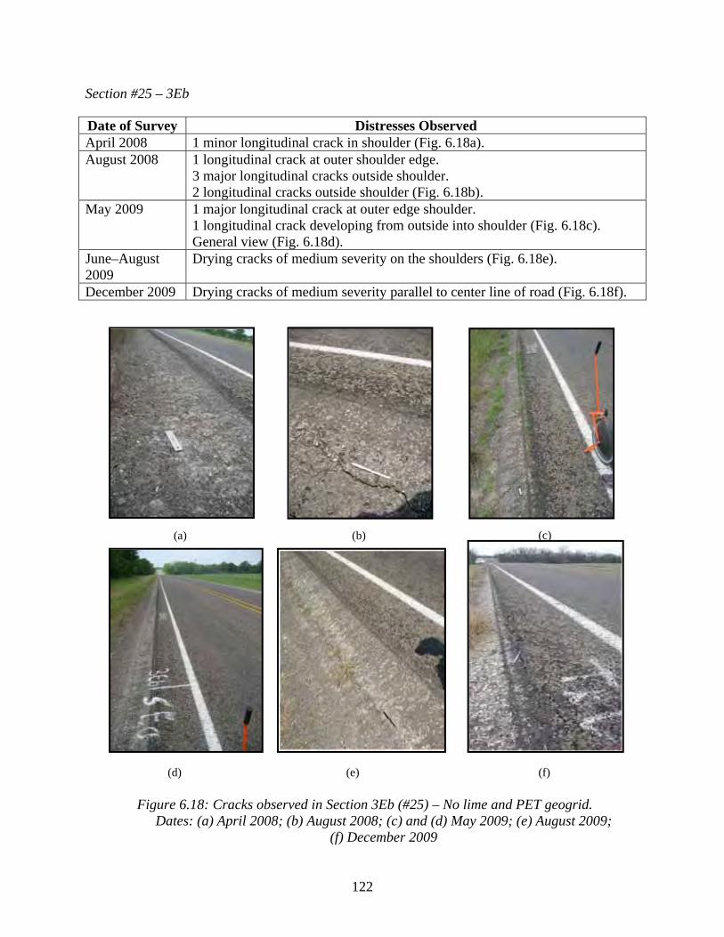
122

Section #25 – 3Eb

Date of Survey Distresses Observed April 2008 1 minor longitudinal crack in shoulder (Fig. 6.18a). August 2008 1 longitudinal crack at outer shoulder edge.

3 major longitudinal cracks outside shoulder. 2 longitudinal cracks outside shoulder (Fig. 6.18b).

May 2009 1 major longitudinal crack at outer edge shoulder. 1 longitudinal crack developing from outside into shoulder (Fig. 6.18c). General view (Fig. 6.18d).

June–August 2009

Drying cracks of medium severity on the shoulders (Fig. 6.18e).

December 2009 Drying cracks of medium severity parallel to center line of road (Fig. 6.18f).

Figure 6.18: Cracks observed in Section 3Eb (#25) – No lime and PET geogrid.

Dates: (a) April 2008; (b) August 2008; (c) and (d) May 2009; (e) August 2009; (f) December 2009

(b) (a) (c)

(d) (e) (f)

123

Section #3 – 3Wa

Date of Survey Distresses Observed April 2008 No cracks. August 2008 1 minor longitudinal crack in shoulder (Fig. 6.19a).

2 major longitudinal cracks outside shoulder (Fig. 6.19b). May 2009 No cracks. High vegetation.

General view (Fig. 6.19c). August 2009 Pothole repair and segregation of pavement surface (Fig. 6.19d) December 2009 No additional distresses observed

Figure 6.19: Cracks observed in Section 3Wa (#3)–No lime and PET geogrid.

Dates: (a) and (b) August 2008;(c) May 2009; (d) August 2009

(b) (a)

(c) (d)

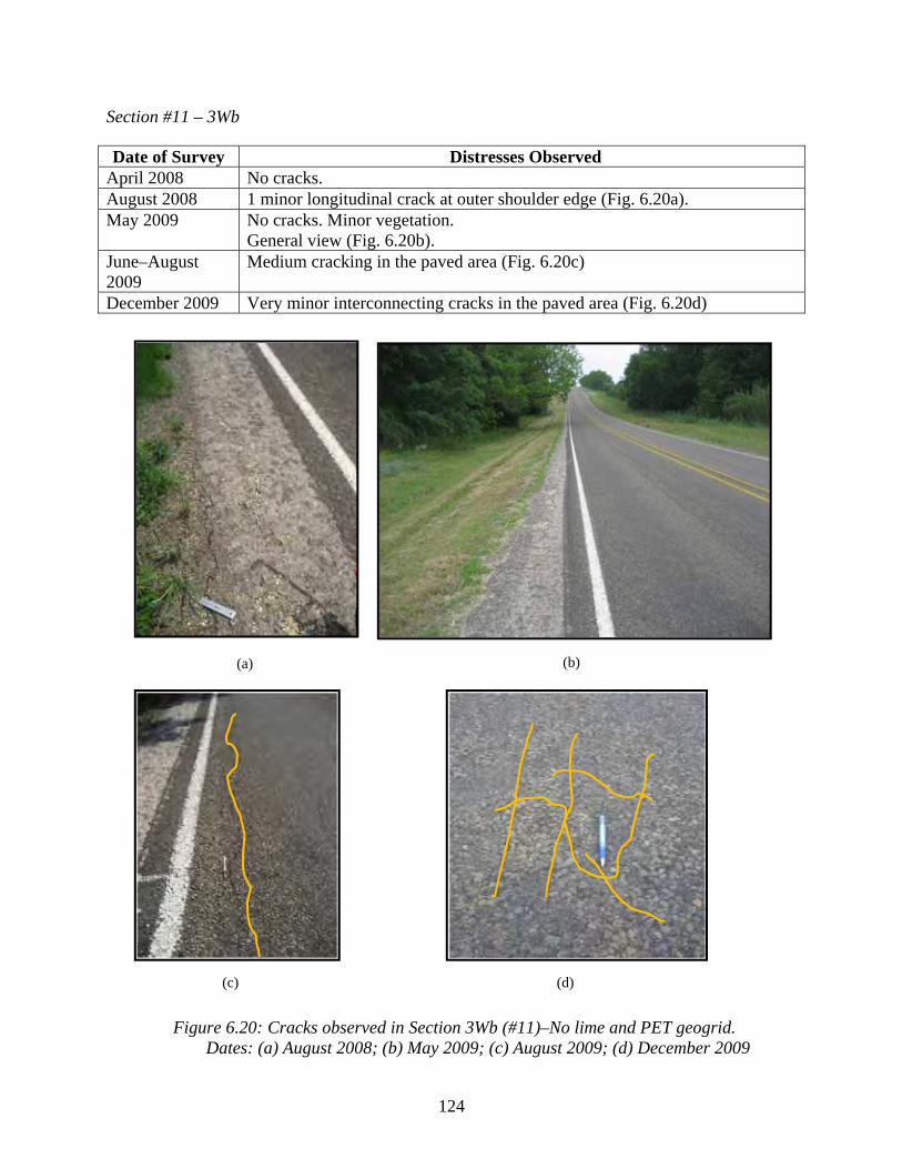
124

Section #11 – 3Wb

Date of Survey Distresses Observed April 2008 No cracks. August 2008 1 minor longitudinal crack at outer shoulder edge (Fig. 6.20a). May 2009 No cracks. Minor vegetation.

General view (Fig. 6.20b). June–August 2009

Medium cracking in the paved area (Fig. 6.20c)

December 2009 Very minor interconnecting cracks in the paved area (Fig. 6.20d)

Figure 6.20: Cracks observed in Section 3Wb (#11)–No lime and PET geogrid.

Dates: (a) August 2008; (b) May 2009; (c) August 2009; (d) December 2009

(b) (a)

(c) (d)

125

6.3.5 Sections with No lime Treatment and Mirafi Geotextile (GT)

Section #19 – 4Ea

Date of Survey Distresses Observed April 2008 No cracks. August 2008 1 major longitudinal crack in shoulder.

2 major longitudinal cracks outside shoulder (Fig. 6.21a). 3 longitudinal cracks outside shoulder.

May 2009 No cracks. High vegetation. General view (Fig. 6.21b). June–Aug 2009 Few longitudinal minor cracks on shoulder December 2009 Minor cracks in the paved area (Fig. 6. 21c).

Figure 6.21: Cracks observed in Section 4Ea (#19)–No lime and PP geotextile.

Dates: (a) August 2008; (b) May 2009; (c) December 2009

(b) (a)

(c)

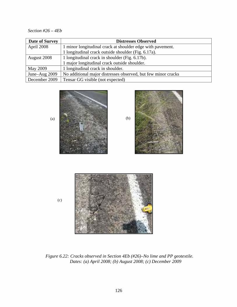
126

Section #26 – 4Eb

Date of Survey Distresses Observed April 2008 1 minor longitudinal crack at shoulder edge with pavement.

1 longitudinal crack outside shoulder (Fig. 6.17a). August 2008 1 longitudinal crack in shoulder (Fig. 6.17b).

1 major longitudinal crack outside shoulder. May 2009 1 longitudinal crack in shoulder. June–Aug 2009 No additional major distresses observed, but few minor cracks December 2009 Tensar GG visible (not expected)

Figure 6.22: Cracks observed in Section 4Eb (#26)–No lime and PP geotextile.

Dates: (a) April 2008; (b) August 2008; (c) December 2009

(b) (a)

(c)

127

Section #4 – 4Wa

Date of Survey Distresses Observed April 2008 No cracks. August 2008 4 major longitudinal cracks outside shoulder (Fig. 6.23a). This crack seems to

exist throughout entire section. May 2009 No cracks. Minor vegetation. General view (Fig. 6.23b). August 2009 Minor cracks begin to originate at many locations (Fig. 6.23c) December 2009 Medium longitudinal cracks in the paved area (Fig. 6.23d)

Figure 6.23: Cracks observed in Section 4Wa (#4)–No lime and PP geotextile.

Dates: (a) August 2008; (b) May 2009

(b) (a)

(d) (c)

128

Section #12 – 4Wb

Date of Survey Distresses Observed April 2008 3 minor longitudinal cracks outside shoulder (Fig. 6.24a). August 2008 1 minor longitudinal crack at outer shoulder edge.

1 major longitudinal crack outside shoulder. 2 minor longitudinal crack in shoulder (Fig. 6.24b).

May 2009 No cracks. High vegetation. General view (Fig. 6.24c). August 2009 Rutting and minor cracking IN the pavement December 2009 Medium longitudinal cracks IN the pavement

Figure 6.24: Cracks observed in Section 4Wb (#12)–No lime and PP geotextile.

Dates: (a) April 2008; (b)August 2008; (c) May 2009

(b) (a)

(c) (d)

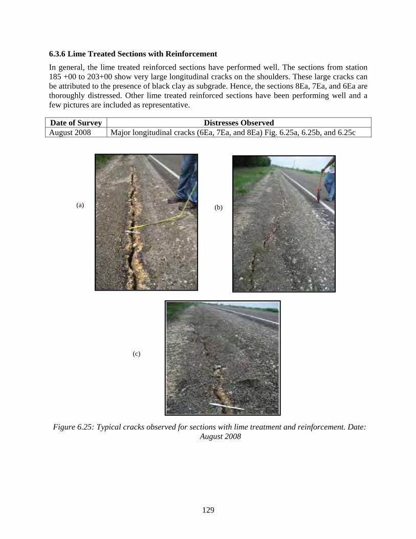
129

6.3.6 Lime Treated Sections with Reinforcement

In general, the lime treated reinforced sections have performed well. The sections from station 185 +00 to 203+00 show very large longitudinal cracks on the shoulders. These large cracks can be attributed to the presence of black clay as subgrade. Hence, the sections 8Ea, 7Ea, and 6Ea are thoroughly distressed. Other lime treated reinforced sections have been performing well and a few pictures are included as representative.

Date of Survey Distresses Observed August 2008 Major longitudinal cracks (6Ea, 7Ea, and 8Ea) Fig. 6.25a, 6.25b, and 6.25c

Figure 6.25: Typical cracks observed for sections with lime treatment and reinforcement. Date:

August 2008

(b) (a)

(c)

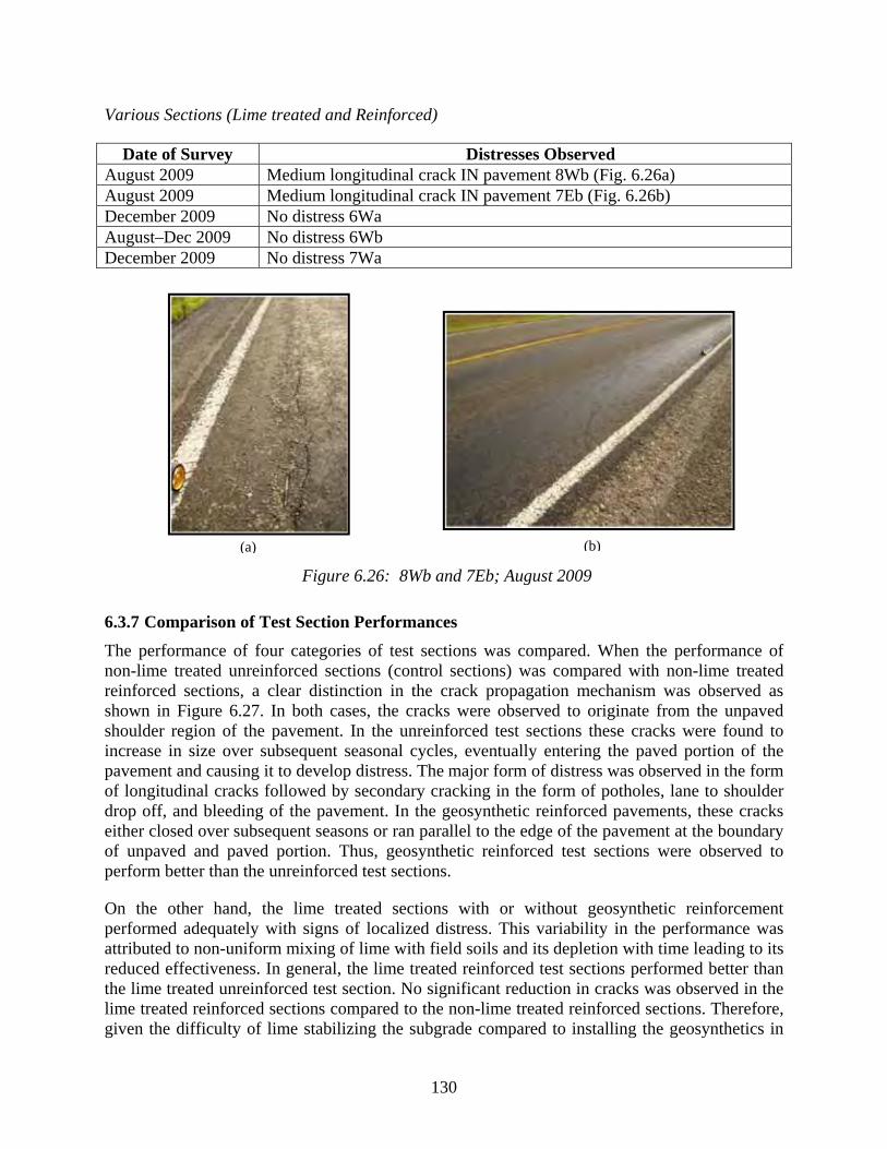
130

Various Sections (Lime treated and Reinforced)

Date of Survey Distresses Observed August 2009 Medium longitudinal crack IN pavement 8Wb (Fig. 6.26a) August 2009 Medium longitudinal crack IN pavement 7Eb (Fig. 6.26b) December 2009 No distress 6Wa August–Dec 2009 No distress 6Wb December 2009 No distress 7Wa

Figure 6.26: 8Wb and 7Eb; August 2009

6.3.7 Comparison of Test Section Performances

The performance of four categories of test sections was compared. When the performance of non-lime treated unreinforced sections (control sections) was compared with non-lime treated reinforced sections, a clear distinction in the crack propagation mechanism was observed as shown in Figure 6.27. In both cases, the cracks were observed to originate from the unpaved shoulder region of the pavement. In the unreinforced test sections these cracks were found to increase in size over subsequent seasonal cycles, eventually entering the paved portion of the pavement and causing it to develop distress. The major form of distress was observed in the form of longitudinal cracks followed by secondary cracking in the form of potholes, lane to shoulder drop off, and bleeding of the pavement. In the geosynthetic reinforced pavements, these cracks either closed over subsequent seasons or ran parallel to the edge of the pavement at the boundary of unpaved and paved portion. Thus, geosynthetic reinforced test sections were observed to perform better than the unreinforced test sections.

On the other hand, the lime treated sections with or without geosynthetic reinforcement performed adequately with signs of localized distress. This variability in the performance was attributed to non-uniform mixing of lime with field soils and its depletion with time leading to its reduced effectiveness. In general, the lime treated reinforced test sections performed better than the lime treated unreinforced test section. No significant reduction in cracks was observed in the lime treated reinforced sections compared to the non-lime treated reinforced sections. Therefore, given the difficulty of lime stabilizing the subgrade compared to installing the geosynthetics in

(b)(a)

131

the field, no clear advantage was observed in terms of performance for the lime stabilized test sections. Overall, the control sections were found to have the highest severity of distress in terms of longitudinal cracks. The use of geosynthetic reinforcement and lime-treatment were observed to help in mitigating the development of such cracks into the main pavement section.

Figure 6.27: Hypothesis for explanation of the mechanisms of the cracks observed in the FM2 road: (a) Unreinforced section (b) Reinforced section

6.3.8 Discussion

The field visual inspection was carried out to document the cracking pattern (origin and spreading) at the site. The longitudinal cracks were observed to originate from the edge of the pavement. Furthermore, the increased evidence of longitudinal cracking was found in the summer seasons. It was envisioned that as the dry front progressed from the edge of the pavement towards the center, the water content in the subgrade below was reduced causing it to shrink thereby opening the cracks. The results obtained by field visual inspection were related with the field moisture data collected from the installed sensors. Both methods indicated that the

Center line

12 ft.

ShoulderPaved portion of pavementStage 1:

Crack initiation at shoulder

Stage 2:Crack propagation

Stage 3:Crack intersecting with unreinforced pavement

Stage 4:Cracking of the pavement

Center line

12 ft.

ShoulderPaved portion of pavementStage 1:

Crack initiation at shoulder

Stage 2:Crack propagation

Stage 3:Crack intersecting with reinforced pavement

Stage 4:Crack parallel to the edge of

pavement

(a)

(b)

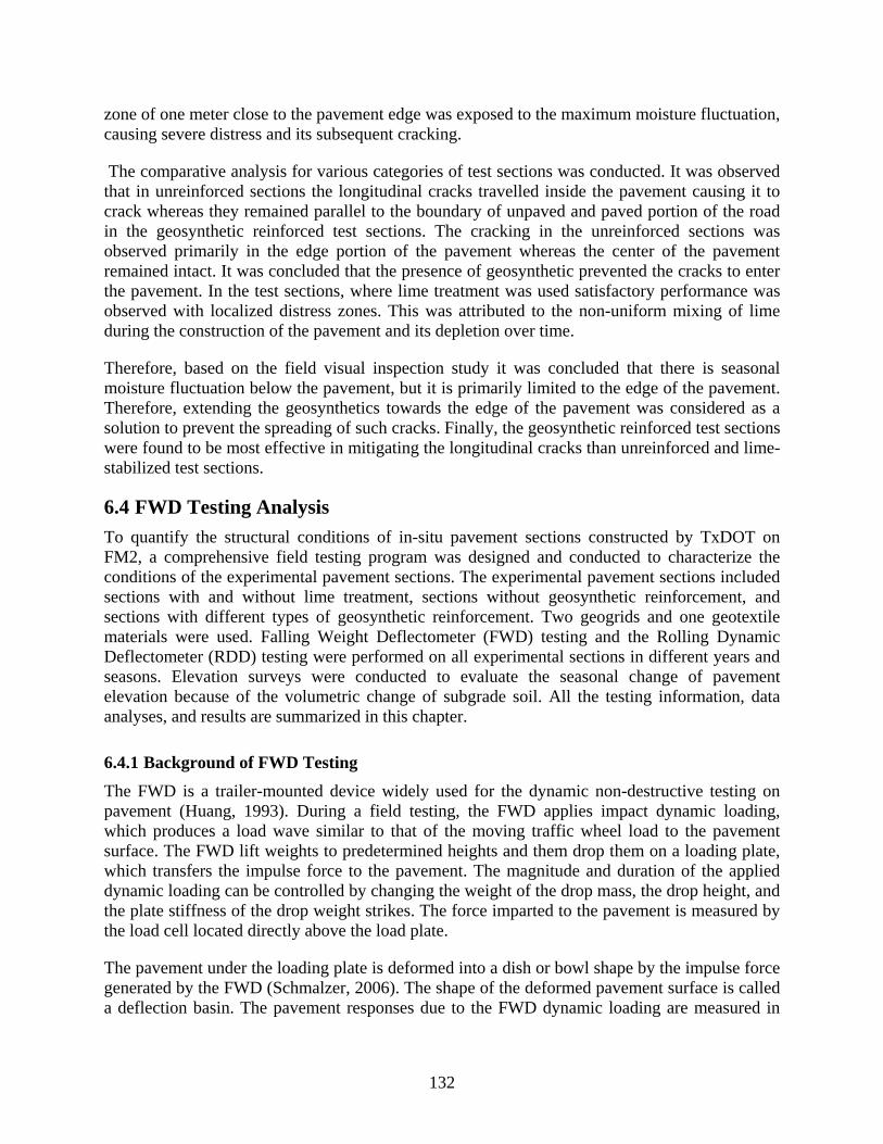
132

zone of one meter close to the pavement edge was exposed to the maximum moisture fluctuation, causing severe distress and its subsequent cracking.

The comparative analysis for various categories of test sections was conducted. It was observed that in unreinforced sections the longitudinal cracks travelled inside the pavement causing it to crack whereas they remained parallel to the boundary of unpaved and paved portion of the road in the geosynthetic reinforced test sections. The cracking in the unreinforced sections was observed primarily in the edge portion of the pavement whereas the center of the pavement remained intact. It was concluded that the presence of geosynthetic prevented the cracks to enter the pavement. In the test sections, where lime treatment was used satisfactory performance was observed with localized distress zones. This was attributed to the non-uniform mixing of lime during the construction of the pavement and its depletion over time.

Therefore, based on the field visual inspection study it was concluded that there is seasonal moisture fluctuation below the pavement, but it is primarily limited to the edge of the pavement. Therefore, extending the geosynthetics towards the edge of the pavement was considered as a solution to prevent the spreading of such cracks. Finally, the geosynthetic reinforced test sections were found to be most effective in mitigating the longitudinal cracks than unreinforced and lime-stabilized test sections.

6.4 FWD Testing Analysis

To quantify the structural conditions of in-situ pavement sections constructed by TxDOT on FM2, a comprehensive field testing program was designed and conducted to characterize the conditions of the experimental pavement sections. The experimental pavement sections included sections with and without lime treatment, sections without geosynthetic reinforcement, and sections with different types of geosynthetic reinforcement. Two geogrids and one geotextile materials were used. Falling Weight Deflectometer (FWD) testing and the Rolling Dynamic Deflectometer (RDD) testing were performed on all experimental sections in different years and seasons. Elevation surveys were conducted to evaluate the seasonal change of pavement elevation because of the volumetric change of subgrade soil. All the testing information, data analyses, and results are summarized in this chapter.

6.4.1 Background of FWD Testing

The FWD is a trailer-mounted device widely used for the dynamic non-destructive testing on pavement (Huang, 1993). During a field testing, the FWD applies impact dynamic loading, which produces a load wave similar to that of the moving traffic wheel load to the pavement surface. The FWD lift weights to predetermined heights and them drop them on a loading plate, which transfers the impulse force to the pavement. The magnitude and duration of the applied dynamic loading can be controlled by changing the weight of the drop mass, the drop height, and the plate stiffness of the drop weight strikes. The force imparted to the pavement is measured by the load cell located directly above the load plate.

The pavement under the loading plate is deformed into a dish or bowl shape by the impulse force generated by the FWD (Schmalzer, 2006). The shape of the deformed pavement surface is called a deflection basin. The pavement responses due to the FWD dynamic loading are measured in

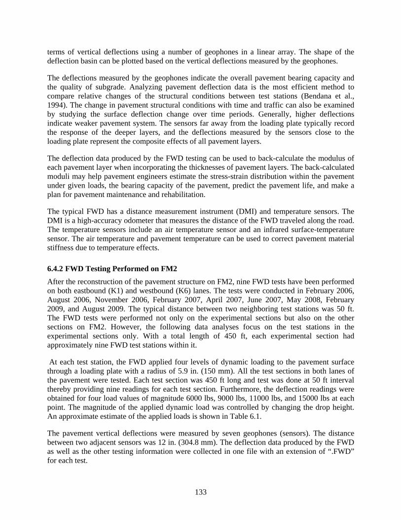
133

terms of vertical deflections using a number of geophones in a linear array. The shape of the deflection basin can be plotted based on the vertical deflections measured by the geophones.

The deflections measured by the geophones indicate the overall pavement bearing capacity and the quality of subgrade. Analyzing pavement deflection data is the most efficient method to compare relative changes of the structural conditions between test stations (Bendana et al., 1994). The change in pavement structural conditions with time and traffic can also be examined by studying the surface deflection change over time periods. Generally, higher deflections indicate weaker pavement system. The sensors far away from the loading plate typically record the response of the deeper layers, and the deflections measured by the sensors close to the loading plate represent the composite effects of all pavement layers.

The deflection data produced by the FWD testing can be used to back-calculate the modulus of each pavement layer when incorporating the thicknesses of pavement layers. The back-calculated moduli may help pavement engineers estimate the stress-strain distribution within the pavement under given loads, the bearing capacity of the pavement, predict the pavement life, and make a plan for pavement maintenance and rehabilitation.

The typical FWD has a distance measurement instrument (DMI) and temperature sensors. The DMI is a high-accuracy odometer that measures the distance of the FWD traveled along the road. The temperature sensors include an air temperature sensor and an infrared surface-temperature sensor. The air temperature and pavement temperature can be used to correct pavement material stiffness due to temperature effects.

6.4.2 FWD Testing Performed on FM2

After the reconstruction of the pavement structure on FM2, nine FWD tests have been performed on both eastbound (K1) and westbound (K6) lanes. The tests were conducted in February 2006, August 2006, November 2006, February 2007, April 2007, June 2007, May 2008, February 2009, and August 2009. The typical distance between two neighboring test stations was 50 ft. The FWD tests were performed not only on the experimental sections but also on the other sections on FM2. However, the following data analyses focus on the test stations in the experimental sections only. With a total length of 450 ft, each experimental section had approximately nine FWD test stations within it.

At each test station, the FWD applied four levels of dynamic loading to the pavement surface through a loading plate with a radius of 5.9 in. (150 mm). All the test sections in both lanes of the pavement were tested. Each test section was 450 ft long and test was done at 50 ft interval thereby providing nine readings for each test section. Furthermore, the deflection readings were obtained for four load values of magnitude 6000 lbs, 9000 lbs, 11000 lbs, and 15000 lbs at each point. The magnitude of the applied dynamic load was controlled by changing the drop height. An approximate estimate of the applied loads is shown in Table 6.1.

The pavement vertical deflections were measured by seven geophones (sensors). The distance between two adjacent sensors was 12 in. (304.8 mm). The deflection data produced by the FWD as well as the other testing information were collected in one file with an extension of “.FWD” for each test.

134

Table 6.1: Estimation of the loads of the FWD tests performed at FM2 road

Drop Load (lb) 1 6000 2 9000 3 11000 4 15000

The 2007 analysis of the FWD deflection data indicated that the lime treated sections had lower deflection values than sections without lime treatment. It also indicated that the geosynthetic-reinforced sections do NOT have better response in terms of deflection. This speculation has turned out to be incorrect looking at the present scenario of the FWD testing data analysis.

6.4.3 Analysis of FWD Deflection Data

As we know, the FWD testing procedure is based on empiricism. The deflection data that we acquire has been used traditionally used for back calculation of the moduli of different layers of the pavement. This approach is based on some primary assumptions like linear elasticity of the asphalt layer, base layer, and sub-base layer. It has consistently been seen that the moduli of similar material bases come out to be dissimilar. The Modulus determination approach is primarily dependent on the initial or seed value the user puts in the program. Also, based on the temperature of asphalt, the program locks the maximum and minimum values of the HMA layer modulus. Thus, varying answers for the same data can be achieved by different users. Thus, this approach is deemed as deceiving. Further, the purported values of moduli of the pavement layers are just an approximation. Hence, most of the moduli back-calculation programs such as WESDEF, MODULUS, and EVERCALC can only be looked at as fair approximations. Though these programs are user friendly and fast, they are certainly not reliable.

The four loadings corresponding to the four drops have been normalized to equivalent single axle load reading of 9,000 lbs. The analysis of the pavement was done assuming it as a linear system. The first deflectometer reading—the deflection from the sensor closest to the dropped weight—is reported in the analysis as it represents the response of the entire pavement section for the given load. The average readings for a group of four sections are as shown in Figure 6.28. The section with lowest deflection for a give load was considered the stiffest and thus performing better than other sections. The details of the deflection profiles observed for different sections over time and their relative performance to each other are discussed.

135

Figure 6.28: FWD data analyses (a) Different load levels at a section (b) Averaged deflections

for a series of test sections for comparison

6.4.4 Performance of Test Sections

The response of the pavement sections for a given load in terms of deflection was measured using FWD tests. The details of test section were described in previous sections. During the field survey, preferential cracking was observed at east side of the pavement as compared to the west side of the pavement due to the location of the test sections. Furthermore, the sections located in the stations from 80+00 to 98+00 had different soil conditions than the main test sections located between stations 185+00 and 203+00. The deflections observed in these sections have been excessive. The reason behind the observed severe deflections basins is the presence of black clay in the subgrade. An analysis that would enable differentiating the behavior of the pavement as regards to its cross-section is still in process. The performance in the form of degradation or improvement in the properties of the different layers of the pavement would be evaluated.

Therefore, in this current account, the performance of first eight sections, i.e., 1Wa to 8Wa as shown in Figure 6.29, is discussed as they were supposed to have the uniform construction and traffic conditions. The sections were divided into four main groups: control section, no reinforcement section with lime treatment (three in numbers), geosynthetic reinforced section with no lime treatment, and geosynthetic reinforced lime treated sections (three in numbers).

0

5

10

15

20

25

30

35

40

45

50

450 500 550 600 650 700 750 800 850 900

Def

lect

ion

(mil

s/ 9

000

lbs)

Station distance (feets)

6000 lbs

9000 lbs

11000 lbs

15000 lbs

450 feet

1 2 3 4 5 6 7 8

Original reading at load of

0

5

10

15

20

25

30

35

40

45

50

0 450 900 1350 1800

Def

lect

ion

(mil

s/ 9

000

lbs)

Station distance (feets)

1Wa 2Wa 3Wa 4Wa

(a)

(b)

136

Figure 6.29: Test sections used in FWD analysis

Finally, for discussion purposes the data obtained from the field trips conducted in February 2006—i.e., immediately after construction of the pavement and the latest one conducted in February 2009—are reported. The deflection profiles for all the above four categories of test section are shown in Figure 6.30a through Figure 6.30d. The deflections increased for all the test sections in the span of three years indicating the structural deterioration of the pavement with time. The test sections where the lime-treatment was used along with geosynthetic reinforcement, no significant change in deflections was observed over the given duration. Thus, for the given pavement this was considered as the best remedial measure to prevent its deterioration due to traffic loading. The performances of test sections relative to each other are compared in subsequent sections.

Control section

(No Lime stabilization, No Geosynthetic reinforcement)221+00

216+50

212+00

207+50

203+00

198+50

194+00

189+50

185+00

Station

2Wa3Wa4Wa

1Wa

6Wa7Wa8Wa

5Wa

K6

Reinforced sections

(No Lime stabilization, Geosynthetic reinforcement only)

Lime treated section

(Lime stabilization only, No Geosynthetic reinforcement)

Lime treated reinforced section

(Lime stabilization and Geosynthetic reinforcement)

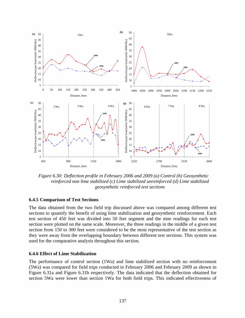
137

Figure 6.30: Deflection profile in February 2006 and 2009 (a) Control (b) Geosynthetic reinforced non lime stabilized (c) Lime stabilized unreinforced (d) Lime stabilized

geosynthetic reinforced test sections

6.4.5 Comparison of Test Sections

The data obtained from the two field trip discussed above was compared among different test sections to quantify the benefit of using lime stabilization and geosynthetic reinforcement. Each test section of 450 feet was divided into 50 feet segment and the nine readings for each test section were plotted on the same scale. Moreover, the three readings in the middle of a given test section from 150 to 300 feet were considered to be the most representative of the test section as they were away from the overlapping boundary between different test sections. This system was used for the comparative analysis throughout this section.

6.4.6 Effect of Lime Stabilization

The performance of control section (1Wa) and lime stabilized section with no reinforcement (5Wa) was compared for field trips conducted in February 2006 and February 2009 as shown in Figure 6.31a and Figure 6.31b respectively. The data indicated that the deflection obtained for section 5Wa were lower than section 1Wa for both field trips. This indicated effectiveness of

5

10

15

20

25

30

35

40

45

50

0 50 100 150 200 250 300 350 400 450

Def

lect

ion

per

load

(mil

s/ 9

00

0 lb

s)

Distance, feets

2006

2009

1Wa

5

10

15

20

25

30

35

40

45

50

450 900 1350 1800

Def

lect

ion

per

load

(mil

s/ 9

00

0 lb

s)

Distance, feets

2006

2009

4 Wa3 Wa2 Wa

5

10

15

20

25

30

35

40

45

50

1800 1850 1900 1950 2000 2050 2100 2150 2200 2250

Def

lect

ion

per

load

(mil

s/ 9

00

0 lb

s)

Distance, feets

2006

2009

5Wa

5

10

15

20

25

30

35

40

45

50

2250 2700 3150 3600

Def

lect

ion

per

load

(mil

s/ 9

00

0 lb

s)

Distance, feets

2006

2009

8 Wa7 Wa6 Wa

(a)(b)

(c) (d)

138

lime treatment in stiffening the pavement thereby reducing the deflection under traffic loading as compared to the control section.

Figure 6.31: Deflection profile for control and lime stabilized unreinforced section for (a) February 2006 (b) February 2009

6.4.7 Effect of Geosynthetic Reinforcement

The performance of three geosynthetic reinforced non-lime treated test sections was compared for field trips conducted in February 2006 and February 2009 as shown in Figure 6.32a and Figure 6.32b respectively. The data indicated that the total deflection obtained for section 2Wa reinforced with geosynthetic G1 was consistently lower than that for section 3Wa and 4Wa reinforced with geosynthetics G2 and G3 for both field trips. The preliminary results based on limited field data obtained for first three years of monitoring the site has shown that the three geosynthetics have performed differently for a given pavement under similar traffic conditions. Still, more field data in terms of FWD deflections is required to make a final assessment of performance for these three test sections and identify the governing distress mode.

The notion of reinforcing pavement with any geosynthetic and achieving the desired benefits is incorrect. Furthermore, the field tests are expensive and time consuming, thus not conducted at regular basis in most of the reinforced pavement projects. Moreover, installing different geosynthetics and observing their performance for a year before constructing the pavement is not a feasible solution.

0

5

10

15

20

25

30

35

40

45

50

0 50 100 150 200 250 300 350 400 450 500

Def

lect

ion

per

load

(mil

s/ 9

00

0 lb

s)

Distance, feets

1Wa

5Wa

February 2009

0

5

10

15

20

25

30

35

40

45

50

0 50 100 150 200 250 300 350 400 450 500

Def

lect

ion

per

load

(mil

s/ 9

00

0 lb

s)

Distance, feets

1Wa

5Wa

February 2006

(a) (b)

139

Figure 6.32: Deflection profile for three geosynthetic reinforced and non- lime stabilized sections for (a) February 2006 (b) February 2009

6.4.8 Effect of Geosynthetic Reinforcement and Lime Stabilization

The performance of three geosynthetic reinforced and lime-treated test sections was compared for field trips conducted in February 2006 and February 2009 as shown in Figure 6.33a and Figure 6.33b respectively. The data indicated that the deflection obtained for these sections was lowest for all the given test sections as discussed earlier. Furthermore, all the three test sections had similar deflection profile immediately after the construction in February 2006. This indicated that in the initial part of the project significant benefit can be obtained by lime treating the pavement. Over the span of three years, the deflection of the pavement increased as indicated by results obtained in February 2009.

Figure 6.33: Deflection profile for three geosynthetic reinforced and lime stabilized sections for (a) February 2006 (b) February 2009

0

5

10

15

20

25

30

35

40

45

50

0 50 100 150 200 250 300 350 400 450 500

Defl

ecti

on

per lo

ad

(m

ils/

90

00

lb

s)

Distance, feets

3Wa2Wa

February 20064Wa

0

5

10

15

20

25

30

35

40

45

50

0 50 100 150 200 250 300 350 400 450 500

Defl

ecti

on

per lo

ad

(m

ils/

90

00

lb

s)

Distance, feets

3Wa

2Wa

February 20094Wa

(a) (b)

0

5

10

15

20

25

30

35

40

45

50

0 50 100 150 200 250 300 350 400 450 500

Def

lect

ion

per

load

(mil

s/ 9

00

0 lb

s)

Distance, feets

7Wa6Wa

February 20068Wa

0

5

10

15

20

25

30

35

40

45

50

0 50 100 150 200 250 300 350 400 450 500

Def

lect

ion

per

load

(mil

s/ 9

00

0 lb

s)

Distance, feets

7Wa

6Wa

February 20098Wa

(a) (b)

140

Furthermore, it was observed that the lime treated test section 6Wa reinforced with geosynthetic G1 had lower deflection than for section 7Wa and 8Wa reinforced with geosynthetics G2 and G3. The similar trend in the performance of three geosynthetics was observed when they were used without lime treatment as discussed in the previous section. However, as observed during the visual inspection the present results indicate that the lime treatment reduces in effectiveness over time and cannot be used as long term remediation strategy by itself. Thus, using lime stabilization along with geosynthetic reinforcement is an effective technique to increase the stiffness of the pavement thereby reducing its deflection under the traffic loads especially over expansive soils.

6.4.9 Discussion

The FWD testing was carried out to quantify the pavement response when it is subjected to traffic loads for the duration of the field study. The results obtained from FWD test done immediately after construction of the pavement in February 2006 were used as the baseline and compared with the latest field test done in February 2009. The results indicated increase in deflection for all the test sections over the span of three years. This showed that the pavement had structurally deteriorated under traffic loads.

The control section had the highest deflection of all the test sections. The lime-treated sections were observed to have stiffer response than non-lime treated sections, immediately after construction. Further, the effect of lime treatment reduced over the three years and increase in deflections was observed, though they were still less than the control section. When the lime treatment was used with geosynthetic reinforcement, the lowest deflections were observed in these test sections indicating it to be a better strategy for reinforcing the expansive soils. In addition to the above study, effect of geosynthetic reinforcement on pavement response was also evaluated. The three geosynthetic reinforced test sections had dissimilar response. Based on preliminary evidences collected so far, it was observed that the test sections reinforced with geosynthetic reinforcement G1 performed better than G2 and G3 independent of the use of lime stabilization in these test sections. The similar order of performance was observed based on laboratory pullout tests reported in terms of coefficient of soil-geosynthetic interaction for these geosynthetics as reported previously.

Based on the field FWD testing it was concluded that there is deterioration of the pavement for traffic loading over the last three years. The lime stabilization may be used as a temporary measure but the geosynthetic reinforcement leads to increase in pavement stiffness over long duration of time. Moreover, different geosynthetics had different response and thus merely using reinforcement would not lead to desired results. Therefore, proper design is required while deciding to use lime stabilization or geosynthetic reinforcement or both for given traffic loads to increase the life span and reduce the maintenance cost for the flexible pavement.

141

References

Abdelouhab, A., Dias, D. Freitag, N. and Bennani, Y., (2008), “Pullout Tests Analytical Modeling to deduce the Constitutive Soil-Reinforcement Interface Behavior,” Paper No. 63, 4th European Conference on Geosynthetics, EuroGeo4, Edinburgh

Abramento, M. and Whittle, A.J., (1995), “Analysis of Pullout Tests for Planar Reinforcements in Soil,” Journal of Geotechnical Engineering, Vol. 121, No. 6, pp. 476-485

Abusaid, A.H. (2006) “Development of a Method to Test Geogrid Reinforcement of Base Materials in Flexible Pavements” M.S. Thesis, Department of Civil Engineering, The University of Texas at Austin

Alfaro, M.C., Miura, N. and Bergado, D.T., (1995), “Soil-geogrid Reinforcement Interaction by Pullout and Direct Shear Tests,” Geotechnical Testing Journal, 18, 157-167

Alobaidi, I.M, Hoare, D.J. and Ghataora, G.S., (1997), “Load Transfer Mechanism in Pullout tests,” Geosynthetics International, Vol. 4, No. 5, pp. 509-521

Al-Qadi, I.L (2006), “Pavement Interlayer System Mechanisms: Separation Reinforcement and Reflective Cracking Control” Lecture, Chinese Society of Pavement Engineering, Taipei, Taiwan, June 2, 2006

Al-Qadi, I.L., Brandon, T.L., and Bhutta, A., (1997), “Geosynthetic Stabilized flexible pavements, “ Proceedings of geosynthetics 97, IFAI, Vol. 2, Long Beach, California, pp.647-662

Al-Qadi, I.L., Brandon, T.L., Valentine, R.J., Lacina, B.A. and Smith, T.E., (1994), “Laboratory Evaluation of Geosynthetic Reinforced Pavement Sections,” Transportation Research Record 1439, pp. 647-662

Al-Qadi, I.L., Dessouky, S.H., Kwon J. and Tutumluer, E. (2008), “Geogrids in Flexible Pavements: Validated Mechanisms,” Transportation Research Record, Journal of the Transportation Research Board, No. 2045, Transportation Research Board of the National Academies, Washington, D.C., 2008. pp. 102-109

American Association of State Highway and Transportation Officials, (1993), “AASHTO Guide for Design of Pavement Structures,” Washington, DC USA

Anderson, P. and Killeavy, M, (1989), “Geotextiles and Geogrids: Cost Effective Alternate Materials for Pavement Design and Construction,” Proceedings of Geosynthetics ’89, IFAI, Vol. 2, Sand Diego, California, USA, February 1989, pp. 353-360

ASTM D2488 (2001), “Standard Practice for Description and Identification of soils (Visual-Manual Procedure),” American Society for Testing and Materials, West Conshohocken, PA

142

ASTM D35 (1995), “ASTM Standards on Geosynthetics,” sponsored by ASTM Committee D-35 on Geosynthetics, Fourth Edition, 178p

ASTM D422 (2007), “Standard Test Method for Particle-Size Analysis of Soils,” American Society for Testing and Materials, West Conshohocken, PA

ASTM D4318 (2001), “Standard Test Methods for Liquid Limit, Plastic Limit and Plasticity Index of Soils,” American Society for Testing and Materials, West Conshohocken, PA

ASTM D4595 (2001), “Standard Test Method for Tensile Properties of Geotextiles by the Wide-Width Strip Method,” American Society for Testing and Materials, West Conshohocken, PA

ASTM D4632 (2008), “Standard Test Method for Grab breaking load and elongation of Geotextiles,” American Society for Testing and Materials, West Conshohocken, PA

ASTM D5311 (2004), “Standard Test Method for Load Controlled Cyclic Triaxial Strength of Soil,” American Society for Testing and Materials, West Conshohocken, PA

ASTM D5617 (2004), “Standard Test Method for Multi-axial Tension test for Geosynthetics,” American Society for Testing and Materials, West Conshohocken, PA

ASTM D6337 (2009), “Standard Test Method for Determining Tensile Properties of Geogrids by the Single or Multi-rib Tensile Method,” American Society for Testing and Materials, West Conshohocken, PA

ASTM D6706 (2003), “Standard Test Method for Measuring Geosynthetic Pullout Resistance in Soil,” American Society for Testing and Materials, West Conshohocken, PA

ASTM D698 (2001), “Standard Test Methods for Laboratory Compaction Characteristics of Soil Using Standard Effort (12400 ft-lbf/ft3 (600 kN-m/m3)),” American Society for Testing and Materials, West Conshohocken, PA

ASTM D854 (2007), “Standard Test Methods for Specific Gravity of Soil Solids by Water Pycnometer,” American Society for Testing and Materials, West Conshohocken, PA

Barker, W.R., (1987), “Open-Graded based for Airfield Pavements,” Technical report GL-87-16, U.S. Army Corps of Engineers, Waterways Experiment Station, Vicksburg, Mississippi, USA, 76p

Barksdale, R.D., Brown, S.F. and Chan, F. (1989), “Potential Benefits of Geosynthetics in Flexible Pavement System,” National Cooperative Highway Research Program, Report No. 315, Transportation Research Board, Nation Research Council, Washington, DC

Bathurst, R.J. (2007) “Geosynthetics Classification.” IGS Leaflets on Geosynthetics Applications, IGS Education Committee, at www.geosyntheticssociety.org.

143

Bay, J.A., and Stokoe, K.H. (1998), “Development of a Rolling Dynamic Deflectometer for Continuous Deflection Measurements of Pavements,” Center of Transportation Research, Report 1422-3F, University of Texas, Austin, TX. 1998.

Bender, D.A. and Barnberg, E.J, (1978), “Design of soil-fabric-aggregate systems,” Transportation Research Record 671, pp 64-75

Benjamin, C.V.S., Bueno, B., Zornberg, J.G., (2007), “Field Monitoring Evaluation of Geotextile-Reinforced Soil Retaining Walls,” Geosynthetics International Journal, April, Vol. 14, No. 1

Berg, R.R., Christopher, B.R. and Perkins, S.W. (2000), “Geosynthetic reinforcement of the aggregate base/subbase courses of flexible pavement structures-GMA white paper II,” Geosynthetic Materials Association, Roseville, MN, USA, 176p.

Bergado, D.T., Teerawattanasuk, C., (2008), “2D and 3D numerical simulations of reinforced embankments on soft ground,” Geotextiles and Geomembranes 26(1), 39–55

Bonaparte, R., Holtz, R.D., and Giroud, J.P., (1987), “Soil reinforcement using Geotextiles and Geogrids,” Geotextile Testing and the Design Engineer, ASTM STP 952, J.E. Fluet, Jr., Ed., American Society for Testing and Materials, Philadelphia, 1987, pp. 69-116

Bray, J.D. and Merry, S.M., (1999), “A comparison of the response of geosynthetics in the multi-axial and uniaxial test devices,” Geosynthetics International, Vol.6, No. 1, pp. 19-40

Brown, S.F., Jones, C.P.D. and Brodrick, B.V., (1982), “ Use of Non-Woven fabrics in permanent road pavements,” Proceedings of the Institution of Civil Engineers, part 2, Vol. 73, pp. 541-563

Bueno, B.S., Benjamin, C.V., and Zornberg, J.G. (2005), “Field Performance of a Full-scale Retaining Wall Reinforced with Non-woven Geotextiles,” Slopes and Retaining Structures under Seismic and Static Conditions, ASCE Geotechnical Special Publication No. 140, January 2005, Austin, Texas (CD-ROM)

Bueno, B.S., Costanzia, M.A., and Zornberg, J.G. (2005), “Conventional and Accelerated Creep Tests on Nonwoven Needle-punched Geotextiles,” Geosynthetics International, December, Vol. 12, No. 6, pp. 276-287

Burd, H.J and Houlsby, G.T. (1986), “A Large Strain Finite Element Formulation for One Dimensional Membrane Elements,” Computers and Geotechnics, Vol. 2, pp. 3-22

Burd, H.J. and Brocklehurst, C.J. (1990), “Finite element studies of the mechanics of reinforced unpaved roads,” Proceedings of the 4th International conference on Geotextiles, Geomembranes and Related Products, The Hague, Netherlands, pp. 217-221

Cancelli, A., Montanelli, F., Rimoldi, P. and Zhao, A., (1996), “Full scale laboratory testing on Geosynthetic reinforced paved roads,” Earth Reinforcement, Ochiai, H., Yasufuku, N., and

144

Omine, K., Editors, Balkema, , Proceeding of the International Symposium on Earth Reinforcement, Fukuoka, Kyushu, Japan, November 1996, pp. 573-578

Chang, J.C., Hannon, J.B., Forsyth, R.A., (1977), “Pullout resistance and interaction of earthwork reinforcement and soil,” Transportation Research Record, 640, National Research Council, Washington D.C. pp. 1-7

Christopher, B.R., Holtz, R.D., and Bell, W.D. (1986), “New tests for determining the In-Soil Stress-Strain properties of Geotextiles,” Proceedings of 3rd International Conference on Geotextiles, Vol. 3, Vienna, pp. 683-688

Collin, J.G., Kinney, T.C. and Fu, X., (1996), “Full scale highway load test of flexible pavement systems with geogrid reinforced base courses,” Geosynthetics International, Vol. 3, No. 4, pp. 537-549

Cuelho, E.L. and Perkins, S.W., (2005), “Resilient interface shear modulus from short-strip cyclic pullout tests,” GSP-140, Slopes and retaining structures under seismic and static conditions, Geofrontiers, Austin, TX

Decagon Devices, (2006), “ECH20 Dielectric Probes vs. Time Domain Reflectometry (TDR),” Application Note

Dondi, G. (1994), “Three-Dimensional Finite Element Analysis of a Reinforced paved Road,” Proceedings of the Fifth International Conference on Geotextiles, Geomembranes and Related Products, Singapore, pp. 95-100

Dougan, Charles (2007), “Mechanistic-Empirical Pavement Design Guide: project Level pavement management” Lecture Session 1a: PMS to support New MEPDG Norfolk, VA, May 7, 2007

Edil, T.B., Kim, W-H., Benson, C.H., Tanyu, B.F., (2007), “Contribution of geosynthetic reinforcement to granular layer stiffness,” GSP 169, Soil and Material inputs for Mechanistic-Empirical Pavement Design, Geo Denver 2007, ASCE

Elias, V., Christopher, B.R. and Berg, R.R., (2001), “Mechanically stabilized earth walls and reinforced soil slopes design and construction guidelines,” National Highway Institute (NHI), Course No 132042, Report No FHWA-NHI-00-043, 394p

Elias, V., Zehong, Y., Swan, R.H. and Bachus, R.C., (1998), “Development of protocols for confined extension and creep testing of geosynthetics for highway applications,” FHWA-RD-97-143, Final report, 201 p.

Fanin, R.J. and Sigurdsson, O., (1996), “Field observations on the stabilization of unpaved roads with geosynthetics,” ASCE Journal of Geotechnical Engineering, Vol. 122(7), 544-553

Fannin, R.J. and Raju, D.M., (1993), “Large scale pullout test results on geosynthetics,” Proceedings of Geosynthetics ʹ93 Conference, Vol. 2, Vancouver, Canada, pp. 633-643

145

Farrag, K., Yalcin A.B., and Juran, I., (1993), “Pullout Resistance of Geogrid Reinforcements,” Geotextiles and Geomembranes, Vol. 12, 133-159

Ferreira J.A.Z., Bueno, B.S. and Zornberg J.G., (2008), “Pavement reinforcement study using small dimensional pullout equipment,” 1st Pan American Geosynthetics Conference, Geoamericas 2008, Cancun, Mexico 2-5 March, 2008

Finnefrock, L.T. (2008) “Bending stiffness index test for geogrid reinforcement of pavement base course material” M.S. Thesis, Department of Civil Engineering, The University of Texas at Austin

Ghionna, V. N., Moraci, N., and Rimoldi, P., (2001), “Experimental evaluation of the factors affecting pullout test results on geogrids,” Proceedings of International Symposium: Earth Reinforcement, Fukuoka, Japan

Giroud, J.P. and Han, J., (2004), “Design method for geogrid-reinforced unpaved roads-1,” Journal of Geotechnical and Geoenvironmental Engineering, Volume 130, Issue 8, pp. 775-786

Giroud, J.P. and Han, J., (2004), “Design method for geogrid-reinforced unpaved roads-II: Calibration and Applications,” Journal of Geotechnical and Geoenvironmental Engineering, Volume 130, Issue 8, pp. 787-797

Giroud, J.P. and Noiray, L., (1981), “Geotextile-Reinforced Unpaved Roads,” Journal of Geotechnical Engineering Division, American Society of Civil Engineers, Vol. 107, No GT9, pp. 1233-1254.

Giroud, J.P., Ah-Line, C., and Bonaparte, R., (1984), “ Design of unpaved roads and trafficked areas with geogrids,” Polymer Grid Reinforcement: A conference sponsored by SERC and Netlon, Ltd., Thomas Telford, London, England, pp. 116-127

Gupta, R., McCartney, J.S., Nogueira, C.L. and Zornberg, J.G., (2008), “Moisture migration in geogrid reinforced expansive subgrades,” Geoamericas 2008, Cancun, Mexico

Halliday, A.R. and Potter, J.F., (1984), “The performance of a flexible pavement constructed on a strong fabric,” Transport and Road Research Laboratory, Report 1123, Crowthorne, Berkshire, United Kingdom, 15p

Haas R., Walls, J. and Carroll, R.G., (1988), “Geogrid Reinforcement of Granular bases in Flexible Pavements,” Transportation Research Record 1188, Washington DC, pp. 19-27

Han, J., Zhang, Y., and Parsons, R.L, (2008), “Development of a performance-based laboratory test method for evaluating geosynthetic-soil confinement,” Geosynthetics Committee (AFS70) TRB 2008 Annual meeting, Washington DC

Hayashi, S., Alfaro, M.C., and Watanbe, K., (1996), “Dilatancy effects of granular soil on the pullout resistance of strip reinforcement,” Proceedings of the International Symposium: Earth Reinforcement, Fukuoka, Kyushu, Japan, pp. 39–44

146

Holtz, R.D, Christopher, B.R. and Berg, R.R, (1998), “Geosynthetic Design and Construction Guidelines,” U.S. Department of Transportation, Federal Highway Administration, Washington, DC, FHWA-HI-98-038, 460 p

Hsieh, C. and Mao, L. (2005), “A bench-scale performance test for evaluation of the geosynthetic reinforcement effects on granular base courses,” GRI-18 Geosynthetics Research and Development in Progress, Geofrontiers, Austin, TX

Huang, Y.H. (1993). Pavement analysis and design, Prentice-Hall, Englewood Cliff, NJ

Hugo, F., McCullough B.F., and Vander Walt B.(1991), “Full-scale accelerated pavement testing for the Texas State Department of Highways and Public Transportation,” Transportation Research Record 1293, Transportation Research Board, National Research Council, Washington, D.C., 1991, pp. 52-60

Ingold, T.S. (1983), “Laboratory pullout testing of grid reinforcement in sand,” Geotechnical Testing Journal, 6 (3), 101-111

Jewell, R.A. (1981), “Some effects of reinforcement on soils,” PhD. Thesis, University of Cambridge, UK

Johnston, R.S. and Romstad, K.M., (1989), “Dilation and boundary effects in large scale pullout tests ,” 12th International Conference on soil Mechanics and Foundation Engineering, Rio de Janeiro, Brazil, Vol. 2, 1263-1266

Juran, I. and Chen, C.L., (1988), “Soil-Geotextile Pullout Interaction Properties: Testing and Interpretation,” Transportation Research Record 1188, 37-47

Kinney, T.C. and Yuan, X. (1995), “Geogrid aperture rigidity by in-plane rotation,” Proceedings of Geosynthetics 1995, pp 525-537

Koerner, R.M. (2005). Designing With Geosynthetics, 5th Edition, Prentice-Hall Inc., Englewood Cliffs, NJ, 1998, 796 p

Konietzky, H., Kamp L., Groeger, T. and Jenner, C, (2004), “Use of DEM to model the interlocking effect of geogrids under static and cyclic loading,” International PFC symposium 28-29 October, 2004, Kyoto, Japan, pp. 3-12

Kupec, J. and McGown, A. (2004), “The load-strain behavior of biaxial geogrids,” Proceedings of 3rd Asian Regional Conference on Geosynthetics, Seoul, South Korea, pp. 349-356

Kwon, J., Tutumluer, E. and Kim, M. (2005), “Development of a mechanistic model for geosynthetic-reinforce flexible pavements,” Geosynthetics International, Vol. 12, No. 6, 310-320

Kwon, J., Tutumluer, E. and Konietzky, H. (2008), “Aggregate base residual stress affecting geogrid reinforced flexible pavement response,” International Journal of Pavement Engineering, Vol. 9, No. 4, August, 2008, pp. 275-285

147

Li, C., (2005), “Mechanical Response of Fiber-Reinforced Soil,” Ph.D. Dissertation, the University of Texas at Austin, Texas, USA

Ling H.I, Wu, J.T.H. and Tatsuoka, F., (19920, “Short-term strength and deformation characteristics of Geotextiles under typical operational conditions,” Geotextiles and Geomembranes, 11 (2), 185-219

Lopes, M.L. and Ladeira, M. (1996), “Influence of the confinement, soil density and displacement ratio on soil-geogrid interaction,” Geotextiles and Geomembranes, 14(10), 543-554

Madhav, M.R., Gurung, N. and Iwao, Y., (1998), “A Theoretical Model for the Pullout Response of Geosynthetic Reinforcement,” Geosynthetics International, Vol. 5, No. 4, pp. 399-424

McDowell, G.R., Harireche, O., Konietzky H., Brown, S.F., and Thom, N.H. (2006), “Discrete element modeling of geogrid-reinforced aggregates,” Proceedings of the Institution of Civil Engineers, Geotechnical Engineering 159, January 2006, Issue GE1, pp.35-48

McGown, A., Andrawes, K.Z. and Al-Hasani, M.M., (1978), “Effect of Inclusion Properties on the Behavior of Sand,” Geotechnique, Vol. 28, No. 3, pp. 327-346

McGown, A., Kupec, J. Heerten, G. and Maubeuge K. von, (2005), “Testing biaxial geogrids for specification and design purposes,” GRI-18 Geosynthetics research and development in progress, ASCE, Austin, Texas

Miller, J.S. and Bellinger, W.Y., (2003), “Distress Identification Manual for the Long-Term Pavement Performance Program, Fourth Revised Edition,” Report No. FHWA-RD-030031, June 2003, 164p

Miura, N., Sakai, A., Taesiri, Y., Yamanouchi, T. and Yasuhara, K., (1990), “Polymer grid reinforced pavement on soft clay grounds,” Geotextiles and Geomembranes, Vol. 9, No. 1, pp. 99-123

Moghaddas-Nejad, F. and Small, J.C., (1996), “Effect of geogrid reinforcement in model track tests on pavements,” Journal of Transportation Engineering, Vol. 122, No. 6, pp. 468-474

Moraci, N., Romano, G., and Montanelli, F., (2004), “Factors affecting the interface apparent coefficient of friction in pullout conditions” 3rd European Geosynthetics Conference, Vol. 1, Monaco, pp. 313-318

Muench, S., (2006), http://pavementinteractive.org/index.php?title=Image:Hma.jpg

NCHRP (2000), NCHRP Project 1-28A, Harmonized Test Methods for Laboratory Determination of Resilient Modulus for Flexible Pavement Design, Volume 1, Unbound Granular Material, 198p

NCHRP (2004), NCHRP Project 1-37A, Guide for Mechanistic-Empirical Design of new and rehabilitated pavement structures, Washington, D.C.

148

Ochiai, H., Otani, J., Hayashic, S., and Hirai, T., (1996), “The pullout resistance of geogrids in reinforced soil,” Geotextiles and Geomembranes, Vol. 14, 19-42

Olidis, C. and Hein, D. (2004), “Guide for Mechanistic-Empirical Design of New and Rehabilitated Pavement Structures: Material Characterization.” Annual Conference of the Transportation Association of Canada, Quebec City, Quebec

Palmeira, E.M. (1987), “The study of soil-reinforcement interaction by means of large scale laboratory tests” PhD. Thesis, University of Oxford, UK, 238p

Palmeira, E.M. (2004), “Bearing force mobilization in pullout tests on geogrids,” Geotextiles and Geomembranes, 22 (6), 481-509

Palmeira, E.M. (2008), “Soil-geosynthetic interaction: Modeling and Analysis,” Mercer Lecture, presented at 4th European Conference on Geosynthetics-EuroGeo4, Edinburgh 2008

Palmeira, E.M. and Milligan, G.W.E., (1989), “Large scale direct shear tests on reinforced sand,” Soils and Foundations, 29(1), 18-30

Palmeira, E.M. and Milligan, G.W.E., (1989), “Scale and other factors affecting the results of pullout tests of grid buried in sand,” Geotechnique, 11 (3), 511–524

Perkins, S.W (2002), “Evaluation of Geosynthetic Reinforced Flexible Pavement systems using two Pavement Test facilities,” Final report, FHWA/MT-02-008/20040, Federal Highway Administration, Washington DC, 120p

Perkins, S.W. (1999), “Geosynthetic reinforcement of flexible pavements: laboratory based pavement test sections,” U.S. Department of Transportation, Federal Highway Administration, Washington DC, Report No. FHWA/MT-99/8106-1, 140p

Perkins, S.W. (1999), “Mechanical Response of Geosynthetic-Reinforced Flexible pavements,” Geosynthetics International, Vol. 6, No. 5, pp. 347-382

Perkins, S.W. (2001), “Numerical Modeling of Geosynthetic Reinforced Flexible Pavements,” Final report, FHWA/MT-01-003/99160-2, 97p

Perkins, S.W. and Cortez, E.R. (2005), “Evaluation of base-reinforced pavements using a heavy vehicle simulator,” Geosynthetic International, Vol. 12, No.2, pp. 86-98

Perkins, S.W. and Cuelho, E.V., (1999), “Soil-geosynthetic interface strength and stiffness relationships from pullout tests” Geosynthetics International, 6(5), 321-346

Perkins, S.W. and Edens, M.Q (2002), “Finite element and distress models for geosynthetic reinforced pavements,” International Journal of Pavement Engineering, Vol. 3, No. 4, pp. 239-250

149

Perkins, S.W. and Ismeik, M., (1997a), "A Synthesis and Evaluation of Geosynthetic Reinforced Base Course Layers in Flexible Pavements: Part I Experimental Work," Geosynthetics International, Vol. 4, No. 6, pp. 549-604.

Perkins, S.W. and Ismeik, M., (1997b), "A Synthesis and Evaluation of Geosynthetic Reinforced Base Course Layers in Flexible Pavements: Part II Analytical Work," Geosynthetics International, Vol. 4, No. 6, pp. 605-621

Perkins, S.W. and Svanø, G. (2004), “ Assessment of interface shear growth from measured geosynthetic strains in a reinforced pavement subject to repeated loads,” In Compendium of Papers CD-ROM, 83rd Transportation Research Board (TRB) Annual Meeting, Washington, DC, 2004

Perkins, S.W., Bowders J.J, Christopher, B.R., and Berg, R.R. (2005), “Advances in geosynthetic reinforcement in pavement systems,” GeoFrontiers, Austin, TX

Perkins, S.W., Christopher, B.R., Cuelho, E.L., Eiksund, G.R., Hoff, I., Schwartz C.W., Svanø, G. and Want, A., (2004), “Development of design methods for geosynthetic reinforced flexile pavements,” FHWA-DTFH61-01-X-00068, Final report, 263p.

Raju, D.M. (1995), “Monotonic and cyclic pullout resistance of geosynthetics,” PhD. Thesis, University of British Columbia, Canada

Reck, N.C. (2009), “Mechanistic empirical design of geogrid reinforced paved flexible pavements,” Jubilee symposium on Polymer Grid Reinforcement, Institute of Civil Engineers, London, England

Rowe, R.K. and Mylleville, B.L.J. (1994), "Analysis and Design of Reinforced Embankments on Soft or Weak Foundations,” Chapter 7 in Soil Structure Interaction: Numerical Analysis and Modeling, (Ed.) J. Bull, E and F.N. Spon (Chapman & Hall), pp. 231-260

Shukla, S.K. (2002), Geosynthetics and their application, 1st edition, Thomas Telford Ltd., 425 p

Sieira, A.C.C.F. Gerscovich, D.M.S., Sayao, A.S.F.J., (2009), “Displacement and load transfer mechanisms of geogrids under pullout condition,” Geotextiles and Geomembranes, Vol. 27, pp. 241-253

Sobhi, S. and Wu, J.T.H., (1996), “An Interface Pullout Formula for Extensible Sheet Reinforcement,” Geosynthetics International, Vol. 3, No. 5, pp. 565-582

Sprague, C.J, Lothspeich, S., Chuck, F., and Goodman, R., (2004), “Geogrid reinforcement of road base aggregate-measuring the confinement benefit,” Proceedings of Geo-Trans 2004 Conference, Los Angeles, 2004, 996 -1005

Sugimoto, M., Alagiyawanna, A.N.M. and Kadoguchi, K. (2001), “Influence of rigid and flexible face on geogrid pullout tests,” Geotextiles and Geomembranes, 19(5), 257-277

150

Sugimoto, M., and Alagiyawanna, A.N.M., (2003), “Pullout behavior of Geogrid by Test and Numerical Analysis,” Journal of Geotechnical and Geoenvironmental Engineering, Vol. 129, No. 4, April 1, 2003, pp. 361-371

Teixeira, S.H.C. (1999), “ Construction and calibration of a large pullout test device,” M.S. Thesis, Department of Geotechnical Engineering, Engineering School of Sao Carlos, University of Sao Paulo (in Portuguese)

Teixeira, S.H.C. (2003), “Estudo da interação solo-geogrelha em testes de arrancamento e a sua aplicação na análise e dimensionamento de maciços reforçados,” PhD. dissertation, Department of Geotechnical Engineering, Engineering School of Sao Carlos, University of Sao Paulo (in Portuguese)

Teixeira, S.H.C., Bueno, B.S. and Zornberg, J.G., (2007), “Pullout Resistance of Individual Longitudinal and Transverse Geogrid Ribs,” Journal of Geotechnical and Geoenvironmental Engineering, Vol. 133, No. 1, January 1, 2007, pp. 37-50

Tensar (2002), “Base reinforcement-Light Aircraft pavement,” Technical memorandum, available at www.tensarcorp.com/uploadedFiles/SPECTRA_TTN_BASE_3.doc

TRI (2001), “In-plane rotational stiffness: Is this a relevant property for base reinforcement of geosynthetics?” Internal report available at www.tri-env.com

Tutumluer, E. and Dawson, A, (2004), “Resilient characterization of compacted aggregate,” PowerPoint from TRB Workshop on describing aggregate behavior for today’s pavements, Washington, DC

Voottipruex, P., Bergado, D.T., Ounjaichon, P., (2000), “Pullout and direct shear resistance of hexagonal wire mesh reinforcement in weathered Bangkok clay,” Geotechnical Engineering Journal, 31(1), 43-62

Wartman, J., Harmanos, D., and Ibanez, P (2005), “Development of a versatile device for measuring the tensile properties of geosynthetic,” Proceeding of GRI-18 Conference, ASCE, Austin, Texas, 4097-4102

Wathugala, G.W., Huang, B. and Pal, S. (1996), “Numerical Simulation of Geosynthetic Reinforced Flexible pavement,” Transportation Research Record 1534, TRB, National Research Council, Washington, DC, USA, pp. 58-65

Watts, G.R.A., and Blackman, D.I. (2009), “Pavement trafficking trials,” Jubilee symposium on Polymer Grid Reinforcement, Institute of Civil Engineers, London, England

Webster, S.L., (1993), “Geogrid reinforced base courses for flexible pavements for light aircraft , test section construction, behavior under traffic, laboratory tests, and design criteria,” Technical report GL-93-6, U.S. Army Corps of Engineers, Waterways Experiment Station, Vicksburg, Mississippi, USA, 86p

151

Williams, N.D. and Houlihan, M.F., (1987), “Evaluation of interface friction properties between geosynthetics and soils,” Geosynthetics Conference, New Orleans, Vol. 2, pp. 616-627

Wilson-Fahmy, R.F., Koerner, R.M., and Sansone, L.J. (1994), “Experimental behavior of polymeric geogrids in pullout,” Journal of Geotechnical Engineering, 120(4), ASCE, USA, 661-677

WSDOT (2007), “Design Parameters for flexible pavements” http://training.ce.washington,edu/wsdot/modulues/04_design_parameters

Yang, K.H, (2009), “Stress distribution within geosynthetic-reinforced soil structures,” Ph.D. Dissertation, the University of Texas at Austin, Texas, USA

Yoder, E.J., and Witczak, M.W., (1975). Principles of pavement design, second edition, John Wiley and Sons, 711p

Yuan, Z. (2005), “Theoretical analysis of bending stiffness test on geosynthetic reinforced base layer,” Proceedings of NAGS/GRI-19 Cooperative Conference, Dec.14-16, Las Vegas, Nevada, 2005

Yuan, Z. and Chua, K.M., (1991), “Analytical Model for Pullout of Soil Reinforcement,” Transportation Research Record 1330, pp. 64-71

Zornberg, J.G, Prozzi, J.A., Gupta, R., Luo, R., McCartney, J.S., Ferreira, J.A.Z. and Nogueira, C., (2008), “Validating mechanisms in geosynthetic reinforced pavements,” Report No. FHWA/TX-08/0-4829-1, submitted to Center of Transportation Research at Austin, February 2008, 247 p.

Zornberg, J.G. and Gupta, R. (2009), “Reinforced pavements over expansive clay subgrades,” 17th International Conference on Soil Mechanics and Geotechnical Engineering, ICSMGE 2009, Alexandria, Egypt

Zornberg, J.G. and Kang, Y., (2005), “Pullout of Geosynthetic Reinforcement with In-plane Drainage Capability,” GRI-18, Geosynthetics Research and Development in Progress, GeoFrontiers 2005, Austin, USA

Zornberg, J.G., (1994), “Performance of Geotextile Reinforced Soil Structures,” Ph.D. Dissertation, Department of Civil Engineering, University of California, Berkeley, California, USA

Zornberg, J.G., Abu-Hejleh, N., and Wang, T. (2001), “Geosynthetic-Reinforced Soil Bridge Abutments in Highway Applications” Geotechnical Fabrics Report, Vol. 19, No. 2, March 2001, pp. 52-55

Zornberg, J.G., and Christopher, B.R. (2006), “Chapter 27: Geosynthetics,” The Handbook of Groundwater Engineering, Jacques W. Delleur (Editor-in-Chief), CRC Press Inc., Boca Raton, Florida

152

Zornberg, J.G., and Christopher, B.R., Editors (2000). Advances in Transportation and Geoenvironmental Systems using Geosynthetics, ASCE Geotechnical Special Publication No. 103, ASCE Press, ISBN 0-7844-0515-8, 422p

Zornberg, J.G., Gupta, R., Prozzi, J.A., and Goehl, D, (2008), “Case histories on geogrid reinforced pavements to mitigate problems associated with expansive subgrade soils,” GeoAmericas 2008, Cancun, Mexico