Geostatistics in Ecology: Interpolating With Known VarianceAuthor(s): G. Philip RobertsonReviewed work(s):Source: Ecology, Vol. 68, No. 3 (Jun., 1987), pp. 744-748Published by: Ecological Society of AmericaStable URL: http://www.jstor.org/stable/1938482 .Accessed: 23/10/2012 12:50

Your use of the JSTOR archive indicates your acceptance of the Terms & Conditions of Use, available at .http://www.jstor.org/page/info/about/policies/terms.jsp

.JSTOR is a not-for-profit service that helps scholars, researchers, and students discover, use, and build upon a wide range ofcontent in a trusted digital archive. We use information technology and tools to increase productivity and facilitate new formsof scholarship. For more information about JSTOR, please contact support@jstor.org.

.

Ecological Society of America is collaborating with JSTOR to digitize, preserve and extend access to Ecology.

http://www.jstor.org

744 NOTES AND COMMENTS Ecology, VoL 68, No, 3

stead of actual rainfall in models of leaf litter decom?

position in deserts.

Acknowledgments: We thank Rick Castetter for as? sistance with fieldwork. A. Roberts gave secretarial as? sistance. We acknowledge support by the Civil Effect Test Operations and A. Morrow at the Nevada Test Site. This work was supported by Contract DE-AC03- 76-SF00012 between the University of California and the U.S. Department of Energy, by Contract DE-AC09- 76SR00-819 between the University of Georgia Insti? tute of Ecology and the U.S. Department of Energy, and by an interagency grant from the Environmental Protection Agency (EPA-IG-D5-681-ACC).

Literature Cited

Comanor, P. L, and E. E. Staffeldt. 1978. Decomposition of plant litter in two western North American deserts. Pages 31-40 in N. E. West and J. J. Skujins, editors. Nitrogen in desert ecosystems, US-IBP Synthesis Series Volume 9. Dowden, Hutchinson and Ross, Stroudsburg, Pennsylva? nia, USA.

El-Ghonemy, A. A., A. Wallace, E. M. Romney, and W. Valentine. 1980. A phytosociological study of a small desert area in Rock Valley, Nevada. Great Basin Naturalist Memoirs 4:59-72.

Franco, P. J., E. B. Edney, and J. F. McBrayer. 1979. The distribution and abundance of soil arthropods in the north? ern Mojave Desert. Journal of Arid Environments 2:137- 149.

French, N. R., B. G. Maza, H. O. Hill, A. P. Aschwanden, and H. W. Kaaz. 1974. A population study of irradiated desert rodents. Ecological Monographs 44:45-72.

Mack, R. N. 1977. Mineral return via the litter of Artemisia tridentata. American Midland Naturalist 97:189-197.

Neter, J., and W. Wasserman. 1974. Applied linear statis? tical models. Richard D. Irwin, Homewood, Illinois, USA.

Santos, P. F, N. Z. Elkins, Y. Steinberger, and W. G. Whit? ford. 1984. A comparison of surface and buried Larrea tridentata leaf litter decomposition in North American hot deserts. Ecology 65:278-284.

Santos, P. F, and W. G. Whitford. 1981. The effects of microarthropods on litter decomposition in a Chihuahuan desert ecosystem. Ecology 62:654-663.

Schaefer, D.A., and W.G. Whitford. 1981. Nutrient cycling by the subterranean termite Gnathamitermes tubiformans in a Chihuahuan Desert ecosystem. Oecologia (Berlin) 48: 277-283.

Strojan, C L., F. B. Turner, and R. Castetter. 1979. Litter fall from shrubs in the northern Mojave Desert. Ecology 60:891-900.

Turner, F. B., editor. 1973. Rock Valley Validation Site report. US-IBP Desert Biome Research Memorandum 73- 2. Utah State University, Logan, Utah, USA.

Whitford, W. G., D. W. Freckman, L. W. Parker, D. Schaefer, P. F. Santos, and Y. Steinberger. 1983. The contribution of soil fauna to nutrient cycles in desert systems. Pages 49- 59 in P. Lebrun, H. M. Andre, A. De Medts, C Gregoire- Wibo, and G. Wauthy, editors. New trends in soil biology. Proceedings ofthe Eighth International Colloquium of Soil Zoology. Dieu-Brichart, Ottignies-Louvain-la-Neuve, France.

1 Manuscript received 16 June 1986; accepted 23 August 1986;

final version received 10 October 1986. 2 Savannah River Ecology Laboratory,

Aiken, South Carolina 29801 USA. 1 Laboratory of Biomedical and Environmental Sciences,

University of California-Los Angeles, Los Angeles, California 90024 USA.

Ecology, 68(3), 1987, pp. 744-748 ? 1987 by the Ecological Society of America

GEOSTA TISTICS IN ECOLOG Y:

INTERPOLATING WITH

KNOWN VARIANCE'

G. Philip Robertson2

Interpolation is perhaps central to most ecological field studies. Ecologists who infer mean values for par? ticular variables within a given experimental plot or time increment implicitly interpolate values for all

points not measured. For example, in systems ecology the mean value for a flux over a landscape unit is

usually based on an average value for randomly dis-

tributed samples within the unit examined. In plant population ecology, estimated population densities are often based on random small-area samplings within the community. So long as assumptions regarding sam?

ple independence and normality are met, parametric statistics for samplings such as these provide optimal estimates of variance about unbiased means, and are

widely used to describe attributes of experimental sites and to test hypotheses about ecological processes at these sites.

Often however, assumptions about sample indepen? dence cannot be met in field studies because of auto- correlation: samples collected close to one another are often more similar to one another than are samples collected farther away, whether in space or time. Con?

sequently, estimates of variance about interpolated points may differ substantially from overall population variance, resulting in imprecise estimates of sample

June 1987 NOTES AND COMMENTS 745

values within the unit sampled (Trangmar et al. 1985) and a biased estimate of treatment effects in experi? mental systems (Sokal and Rohlf 1981). In many field studies such autocorrelation can arise from subtle to-

pographic features of a site that affect a host of other environmental factors such as microclimate or soil nu? trient status; in other studies lack of sample indepen- dence may reflect distance from a major seed, predator, or herbivore source. In studies that involve sampling through time, autocorrelation can result from under?

lying temporal features ofthe system such as diel trends in temperature, radiation, or some other factor not

readily identified and thus not readily treated as a co? variate.

The recent development of regionalized variable the?

ory (Matherton 1971) for applications in geology (e.g., Journel and Huijbregts 1978, Krige 1981) and soil sci? ence (e.g., Burgess and Webster 1980a) provides an

elegant means for describing autocorrelation in data, and a means to use knowledge about this autocorre? lation to derive precise, unbiased estimates of sample values within the sampling unit and thereby resolve detailed spatial and temporal patterns with known variance for each interpolated point. The development of this theory should be of considerable interest to

ecologists. Spatial variability in particular has long been difficult to quantify in ecologically meaningful ways: conventional interpolation techniques such as proxi- mal weighting, trend surface analysis, and spline in?

terpolation do not consistently provide unbiased es? timates for the points interpolated, nor do they esti? mate optimal variances for the interpolated values. Such imprecision leads to questions of statistical con? fidence and subsequent difficulty with the interpreta- tion of the patterns defined. Geostatistical techniques address these problems directly.

Excellent reviews of regionalized variable theory and its strengths and limitations exist already (Krige 1981, Vieiraetal. 1983, Trangmar etal. 1985, Webster 1985). Rather than repeat these discussions, in this note I

present an overview of the theory as it applies to the

analyses of two ecological data sets. The first data set is from a study of temporal changes in Rhodomonas

(Cryptophyceae) density in the epilimnion of a tem?

perate hardwater lake; the second is from an investi-

gation ofthe spatial variability of soil mineral nitrogen in a Michigan old-field community. In addition to de-

scriptions of these analyses I provide a set of FOR- TRAN algorithms that allow straightforward access to these new statistical tools.

Approach and Examples

In its simplest form, geostatistical analysis is a two-

step process: (1) defining the degree of autocorrelation

among the measured data points, and (2) interpolating values between measured points based on the degree of autocorrelation encountered. Autocorrelation is evaluated by means of the semi-variance statistic

7 (h), calculated for each specific distance or time interval h in a data set such that

i N(h) *<h> =

T^TT 2 W*/) ~ *(*/+h)]2 (1) 2N(h) /=1

where z(x) is the measured sample value at point xh z(xi+h) is tne sample value at point xi+h, and N(h) is the total number of sample point contrasts or couples for the interval in question. The resulting plot of 7(h) vs. all h's evaluated is termed the semi-variogram; the

shape of this plot describes the degree of autocorrela? tion present.

Once spatial or temporal dependency is established, one can use semi-variogram parameters to interpolate values for points not measured using kriging algo- rithms. There are several different forms of kriging (Trangmar et al. 1985); the simplest are punctual and block kriging. In punctual kriging, values for exact points within the sampling unit are estimated; block kriging involves estimating values for areas within the unit. Block interpolation (Burgess and Webster 1980Z?) may be more appropriate than punctual interpolation where

average values of properties are more meaningful than exact single-point values, especially where spatial or

temporal dependence is weak. Both forms of kriging provide an error term (esti-

mation variance) for each value estimated, providing a measure of reliability for the interpolations. These error terms are independent of the observed sample values themselves; estimation error depends only on the locations of samples within the range of sample interdependence and on the degree of this dependence as quantified by the semi-variogram. Consequently, kriging can also be used before sampling to design an

optimal strategy for sampling an area or time series

knowing only something about the degree of sample interdependence (the shape ofthe semi-variogram) for

samples within the interpolation domain. For example, where samples are strongly autocorrelated over small

sampling intervals, pre-sample kriging can show where to add sample points to bring estimation precision to a desirable level in sparsely sampled regions. Con-

versely, where samples are weakly autocorrelated over small intervals, pre-sample kriging can show that ad? ditional sampling in a given region will add little ad? ditional precision to interpolation estimates.

Fig. la is a semi-variogram for the temporal Rho- domonas data collected for the study mentioned ear? lier. These data represent cell counts of Rhodomonas

sp. in water samples taken from the epilimnion of Law-

746 NOTES AND COMMENTS Ecology, Vol. 68, No. 3

7000

6000

5000

4000

3000

2000

1000

0

(a)

12 h (days)

20 24

20 40 60 Days

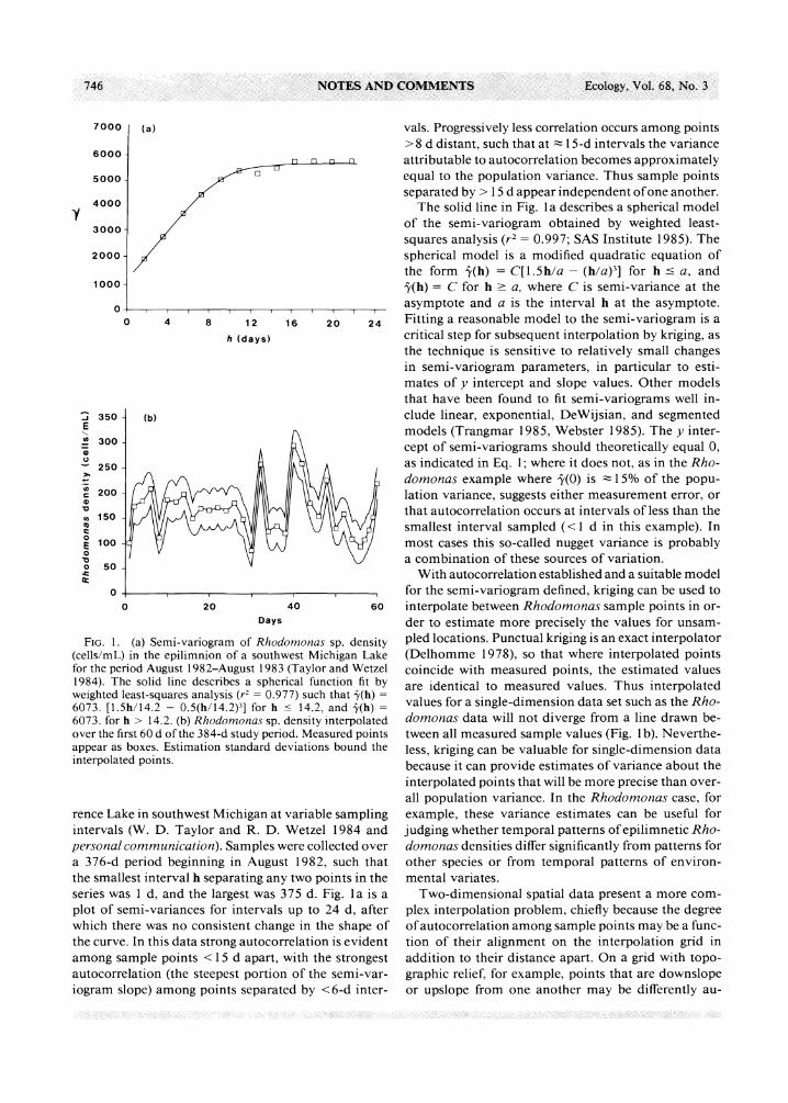
Fig. 1. (a) Semi-variogram of Rhodomonas sp. density (cells/mL) in the epilimnion of a southwest Michigan Lake for the period August 1982-August 1983 (Taylor and Wetzel 1984). The solid line describes a spherical function fit by weighted least-squares analysis (r2 = 0.977) such that -y(h) = 6073. [1.5h/14.2 - 0.5(h/14.2)3] for h < 14.2, and 7(h) = 6073. for h > 14.2. (b) Rhodomonas sp. density interpolated over the first 60 d ofthe 384-d study period. Measured points appear as boxes. Estimation standard deviations bound the interpolated points.

rence Lake in southwest Michigan at variable sampling intervals (W. D. Taylor and R. D. Wetzel 1984 and

personal communication). Samples were collected over a 376-d period beginning in August 1982, such that the smallest interval h separating any two points in the series was 1 d, and the largest was 375 d. Fig. la is a

plot of semi-variances for intervals up to 24 d, after which there was no consistent change in the shape of the curve. In this data strong autocorrelation is evident

among sample points < 15 d apart, with the strongest autocorrelation (the steepest portion of the semi-var?

iogram slope) among points separated by <6-d inter-

vals. Progressively less correlation occurs among points >8 d distant, such that at ? 15-d intervals the variance attributable to autocorrelation becomes approximately equal to the population variance. Thus sample points separated by > 15 d appear independent of one another.

The solid line in Fig. la describes a spherical model of the semi-variogram obtained by weighted least-

squares analysis (r2 = 0.997; SAS Institute 1985). The

spherical model is a modified quadratic equation of the form 7(h) = C[\.5h/a - (h/a)3] for h < a, and

7(h) = C for h > a, where C is semi-variance at the

asymptote and a is the interval h at the asymptote. Fitting a reasonable model to the semi-variogram is a critical step for subsequent interpolation by kriging, as the technique is sensitive to relatively small changes in semi-variogram parameters, in particular to esti? mates of y intercept and slope values. Other models that have been found to fit semi-variograms well in? clude linear, exponential, DeWijsian, and segmented models (Trangmar 1985, Webster 1985). The y inter?

cept of semi-variograms should theoretically equal 0, as indicated in Eq. 1; where it does not, as in the Rho- domonas example where 7(0) is ~ 15% of the popu? lation variance, suggests either measurement error, or that autocorrelation occurs at intervals of less than the smallest interval sampled (<1 d in this example). In most cases this so-called nugget variance is probably a combination of these sources of variation.

With autocorrelation established and a suitable model for the semi-variogram defined, kriging can be used to

interpolate between Rhodomonas sample points in or? der to estimate more precisely the values for unsam-

pled locations. Punctual kriging is an exact interpolator (Delhomme 1978), so that where interpolated points coincide with measured points, the estimated values are identical to measured values. Thus interpolated values for a single-dimension data set such as the Rho? domonas data will not diverge from a line drawn be? tween all measured sample values (Fig. 1 b). Neverthe?

less, kriging can be valuable for single-dimension data because it can provide estimates of variance about the

interpolated points that will be more precise than over? all population variance. In the Rhodomonas case, for

example, these variance estimates can be useful for

judging whether temporal patterns of epilimnetic Rho? domonas densities differ significantly from patterns for other species or from temporal patterns of environ? mental variates.

Two-dimensional spatial data present a more com?

plex interpolation problem, chiefly because the degree of autocorrelation among sample points may be a func? tion of their alignment on the interpolation grid in addition to their distance apart. On a grid with topo- graphic relief, for example, points that are downslope or upslope from one another may be differently au-

June 1987 NOTES AND COMMENTS 747

0.14

0.12

0.10

y 0.08

0.06

0.04

0.02

10 20 30 40 50

h (metres)

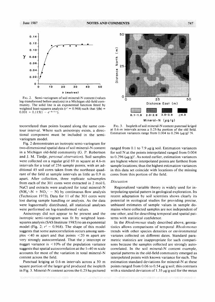
Fig. 2. Semi-variogram of soil mineral-N content (values log-transformed before analysis) in a Michigan old-field com? munity. The solid line is an exponential function fitted by weighted least-squares analysis (r2 = 0.968) such that 7(h) = 0.001 + 0.115(1 - e~h/lil).

tocorrelated than points located along the same con- tour interval. Where such anisotropy exists, a direc- tional component must be included in the semi-

variogram model.

Fig. 2 demonstrates an isotropic semi-variogram for two-dimensional spatial data of soil mineral-N content in a Michigan old-field community (G. P. Robertson and J. M. Tiedje, personal observation). Soil samples were collected on a regular grid 69 m square at 4.6-m intervals for a total of 256 sample points, with an ad? ditional 45 soil cores taken from the northeast quad- rant ofthe field at sample intervals as little as 0.9 m

apart. After collection, three replicate subsamples from each of the 301 cores were extracted in 2 mol/L NaCl and extracts were analyzed for total mineral-N

(NH/-N + N03" ? N) by continuous flow analysis (Technicon 1973). Data for 11 ofthe 301 cores were lost during sample handling or analysis. As the data were lognormally distributed, all statistical analyses were performed on log-transformed values.

Anisotropy did not appear to be present and the

isotropic semi-variogram was fit by weighted least-

squares analysis (SAS Institute 1985) to an exponential model (Fig. 2; r2 = 0.968). The shape of this model

suggests that some autocorrelation occurs among sam?

ples <40 m apart and that points <20 m apart are

very strongly autocorrelated. That the y intercept or

nugget variance is < 10% of the population variance

suggests that spatial autocorrelation at the 1-40 m scale accounts for most of the variation in total mineral-N content across the field.

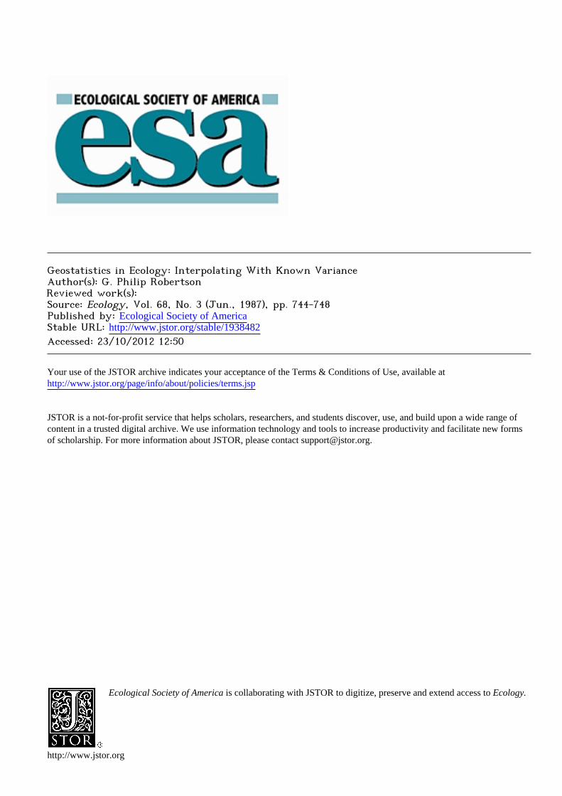
Punctual kriging at 0.6-m intervals across a 50 m

square portion of the larger grid produced the isopleth in Fig. 3. Mineral-N content across the 0.25 ha pictured

25 Distance East (m)

0.1-1.9 2.0-2.9 3.0-3.9 >4.0

Mineral-N (//g/g) Fig. 3. Isopleth of soil mineral-N content punctual kriged

at 0.6-m intervals across a 0.25-ha portion of the old field. Estimation variances range from 0.004 to 0.296 (Mg/g)2 N.

ranged from 0.1 to 7.9 fig/g soil. Estimation variances for soil N at the points interpolated ranged from 0.004 to 0.296 (jiig/g)2. As noted earlier, estimation variances are highest where interpolated points are farthest from

sample locations; thus the highest estimation variances in this data set coincide with locations of the missing cores from this portion of the field.

Discussion

Regionalized variable theory is widely used for in-

terpolating spatial pattern in geological exploration. Its recent adaptation by soil scientists shows clearly its

potential in ecological studies for providing precise, unbiased estimates of sample values in sample do- mains where collected samples are not independent of one other, and for describing temporal and spatial pat? terns with statistical confidence.

In the Rhodomonas study described above, geosta- tistics allows comparisons of temporal Rhodomonas trends with other species densities or environmental variates collected on different dates. Standard para- metric statistics are inappropriate for such compari? sons because the samples collected are strongly auto? correlated. In the soil mineral-N content example, spatial patterns in the old-field community emerged as

interpolated points with known variance for each. The estimation standard deviations for mineral-N at these

points ranged from 0.06 to 0.54 fxg/g soil; this contrasts with a standard deviation of 1.35 jug/g soil for the mean

748 NOTES AND COMMENTS Ecology, Voi. 68, No. 3

mineral-N content (2.67 ng/g soil) of all points sam?

pled. Ecological studies that produce data not amenable

to normal statistical treatment because of spatial or

temporal autocorrelation may significantly benefit from

geostatistical analysis. Autocorrelation is a potential problem in many if not most field sampling strategies, and its presence should be routinely evaluated. The

application of geostatistics to studies with data that exhibit autocorrelation and to studies dealing explicitly with spatial or temporal patterning may substantially aid their interpretation.

FOR TRAN Algorithms

The analyses described above were performed using a set of algorithms written for interactive use on mi-

crocomputers. The algorithms are written in Microsoft

FORTRAN, a subset of the ANSI-77 FORTRAN Standard designed to operate on MS-DOS microcom-

puters but compatible with most mainframe compilers. Source code listings (~6000 lines) are available in

printed form3 or on diskette from the W. K. Kellogg Biological Station Computer Lab.4 Documentation files that accompany the programs provide instructions for their use; users should refer to Vieira et al. (1983), Trangmar et al. (1985), and Webster (1985) for dis- cussions of how to interpret algorithm results.

Acknowledgments: I thank P. Sollins, G. G. Parker, and S. R. Vieira for many helpful comments on an earlier version of this manuscript, T. B. Parkin, B. B.

Trangmar, and R. L. Hill for generously providing al?

gorithms and data against which to test the computer programs developed in this study, and W. Brisky for

programmingexpertise. W. D. Taylor and R. G. Wetzel

3 See ESA Supplementary Publication Service Document No. 8733 for 90 pages of supplementary material. For a copy of this document, contact the author or order from The Eco? logical Society of America, 328 E. State, Ithaca, New York 14850-4318 USA.

4 Source code and documentation on two 5.25-inch, IBM- compatible diskettes are available from the Computer Lab? oratory, W. K. Kellogg Biological Station, Michigan State University, Hickory Corners, Michigan 49060 USA. Please include a $ 12.00 handling fee payable to Michigan State Uni? versity.

kindly provided Rhodomonas data beyond that cited.

Principal support was provided by NSF grant BSR 83- 17198. Contribution Number 591 ofthe W. K. Kellogg Biological Station.

Literature Cited

Burgess, T. M., and R. Webster. 1980<2. Optimal interpo? lation and isarithmic mapping of soil properties. I. The semi-variogram and punctual kriging. Journal of Soil Sci? ence 31:315-331.

Burgess, T. M., and R. Webster. 19806. Optimal interpo? lation and isarithmic mapping of soil properties. II. Block kriging. Journal of Soil Science 31:333-341.

Delhomme, J. P. 1978. Kriging in the hydrosciences. Ad? vances in Water Research 1:251-266.

Journel, A. G., and C. J. Huijbregts. 1978. Mining geosta- tistics. Academic Press, London, England.

Krige, D. G. 1981. Lognormal-de Wijsian geostatistics for ore evaluation. South African Institute of Mining and Met- allurgy Monograph Series. Geostatistics 1. South Africa In? stitute of Mining and Metallurgy, Johannesburg, South Af? rica.

Matherton, G. 1971. The theory of regionalized variables and its applications. Cahiers du Centre de Morphologie Mathematique, Fontainebleau, Numero 5. Ecole Nationale Superieure des Mines de Paris, Paris, France.

SAS Institute. 1982. SAS user's guide: statistics. SAS Insti? tute, Cary, North Carolina, USA.

Sokal, R. R., and F. J. Rohlf. 1981. Biometry. Second edi? tion. W. H. Freeman, San Francisco, California, USA.

Taylor, W. D., and R. G. Wetzel. 1984. Population dynam? ics of Rhodomonas minuta v. nannoplanctica Skuja (Cryp- tophyceae) in a hardwater lake. Internationale Vereinigung fur theoretische und angewandte Limnologie, Verhand? lungen 22:536-541.

Technicon. 1973. Nitrite and nitrate in water and waste- water. Industrial Method Number 100-70W. Technicon Instruments, Tarrytown, New York, USA.

Trangmar, B. B., R. S. Yost, and G. Uehara. 1985. Appli? cation of geostatistics to spatial studies of soil properties. Pages 45-94 in N. C Brady, editor. Advances in agronomy. Volume 38. Academic Press, New York, New York, USA.

Vieira, S. R., J. L. Hatfield, D. R. Nielsen, and J. W. Biggar. 1983. Geostatistical theory and application to variability of some agronomical properties. Hilgardia 51:1-75.

Webster, R. 1985. Quantitative spatial analysis of soil in the field. Pages 1-70 in B. A. Stewart, editor. Advances in soil science. Volume 3. Springer-Verlag, New York, New York, USA.

1 Manuscript received 1 April 1986; revised 1 October 1986; accepted 16 October 1986. 2 W. K. Kellogg Biological Station, Michigan State

University, Hickory Corners, Michigan 49060-9516 USA.