Embed Size (px)
Citation preview
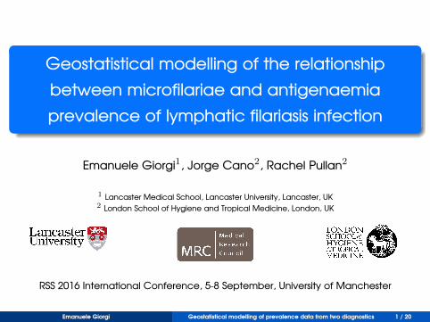
Geostatistical modelling of the relationship
between microfilariae and antigenaemia
prevalence of lymphatic filariasis infection
Emanuele Giorgi1, Jorge Cano2, Rachel Pullan2
1 Lancaster Medical School, Lancaster University, Lancaster, UK2 London School of Hygiene and Tropical Medicine, London, UK
RSS 2016 International Conference, 5-8 September, University of Manchester
Emanuele Giorgi Geostatistical modelling of prevalence data from two diagnostics 1 / 20
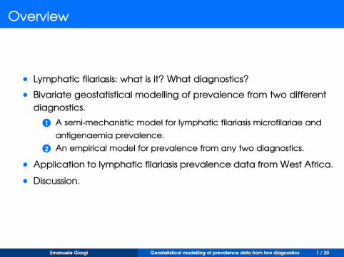
Overview
• Lymphatic filariasis: what is it? What diagnostics?
• Bivariate geostatistical modelling of prevalence from two different
diagnostics.
1 A semi-mechanistic model for lymphatic filariasis microfilariae and
antigenaemia prevalence.
2 An empirical model for prevalence from any two diagnostics.
• Application to lymphatic filariasis prevalence data from West Africa.
• Discussion.
Emanuele Giorgi Geostatistical modelling of prevalence data from two diagnostics 1 / 20
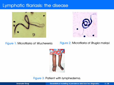
Lymphatic filariasis: the disease
Figure 1: Microfilaria of Wuchereria. Figure 2: Microfilaria of Brugia malayi.
Figure 3: Patient with lymphedema.
Emanuele Giorgi Geostatistical modelling of prevalence data from two diagnostics 2 / 20
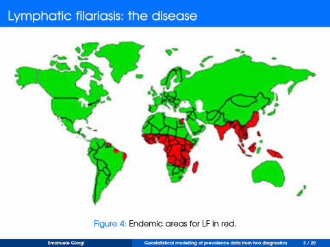
Lymphatic filariasis: the disease
Figure 4: Endemic areas for LF in red.
Emanuele Giorgi Geostatistical modelling of prevalence data from two diagnostics 3 / 20
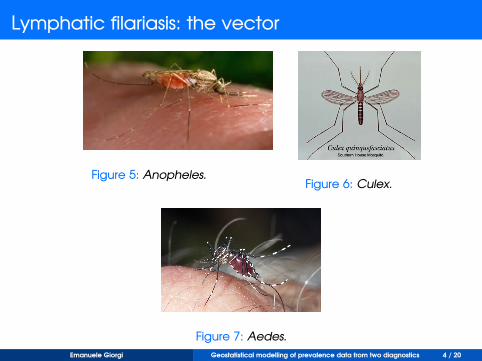
Lymphatic filariasis: the vector
Figure 5: Anopheles.Figure 6: Culex.
Figure 7: Aedes.
Emanuele Giorgi Geostatistical modelling of prevalence data from two diagnostics 4 / 20

Lymphatic filariasis: the life cycle
Figure 8: Life Cycle of Wuchereria bancrofti.
Emanuele Giorgi Geostatistical modelling of prevalence data from two diagnostics 5 / 20
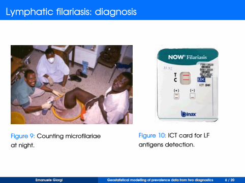
Lymphatic filariasis: diagnosis
Figure 9: Counting microfilariae
at night.
Figure 10: ICT card for LF
antigens detection.
Emanuele Giorgi Geostatistical modelling of prevalence data from two diagnostics 6 / 20
Research question
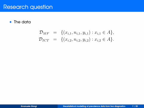
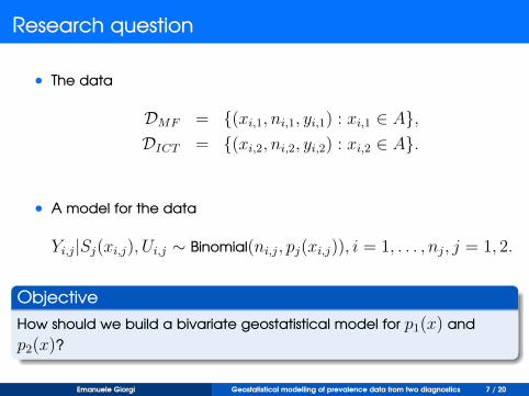
• The data
DMF = {(xi,1, ni,1, yi,1) : xi,1 ∈ A},DICT = {(xi,2, ni,2, yi,2) : xi,2 ∈ A}.
• A model for the data
Yi,j|Sj(xi,j), Ui,j ∼ Binomial(ni,j, pj(xi,j)), i = 1, . . . , nj, j = 1, 2.
Objective
How should we build a bivariate geostatistical model for p1(x) and
p2(x)?
Emanuele Giorgi Geostatistical modelling of prevalence data from two diagnostics 7 / 20

Research question
• The data
DMF = {(xi,1, ni,1, yi,1) : xi,1 ∈ A},DICT = {(xi,2, ni,2, yi,2) : xi,2 ∈ A}.
• A model for the data
Yi,j|Sj(xi,j), Ui,j ∼ Binomial(ni,j, pj(xi,j)), i = 1, . . . , nj, j = 1, 2.
Objective
How should we build a bivariate geostatistical model for p1(x) and
p2(x)?
Emanuele Giorgi Geostatistical modelling of prevalence data from two diagnostics 7 / 20

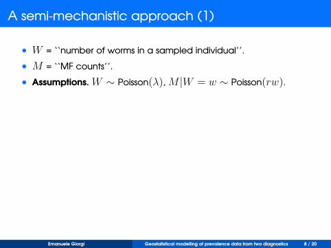
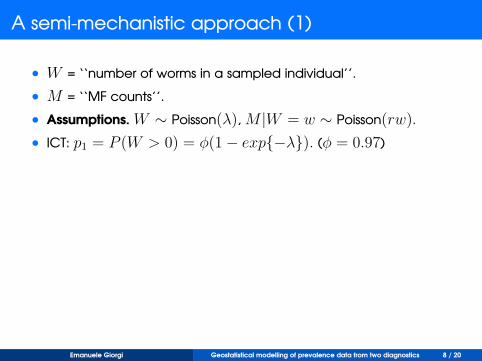
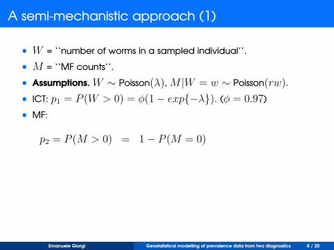
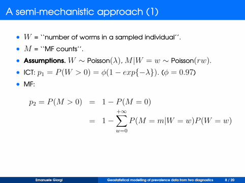
A semi-mechanistic approach (1)
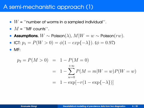
• W = ‘‘number of worms in a sampled individual’’.
• M = ‘‘MF counts’’.
• Assumptions. W ∼ Poisson(λ), M |W = w ∼ Poisson(rw).
• ICT: p1 = P (W > 0) = φ(1− exp{−λ}). (φ = 0.97)
• MF:
p2 = P (M > 0) = 1− P (M = 0)
= 1−+∞∑w=0
P (M = m|W = w)P (W = w)
= 1− exp[−r(1− exp{−λ})]= 1− exp[−rφ−1p1]
Emanuele Giorgi Geostatistical modelling of prevalence data from two diagnostics 8 / 20
A semi-mechanistic approach (1)
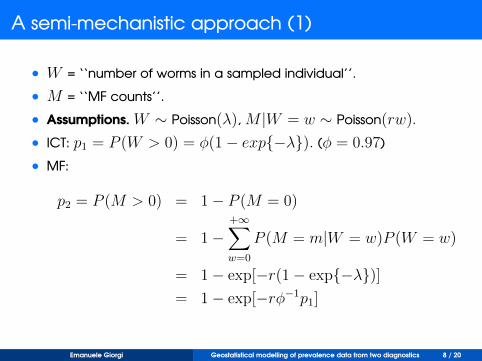
• W = ‘‘number of worms in a sampled individual’’.
• M = ‘‘MF counts’’.
• Assumptions. W ∼ Poisson(λ), M |W = w ∼ Poisson(rw).
• ICT: p1 = P (W > 0) = φ(1− exp{−λ}). (φ = 0.97)
• MF:
p2 = P (M > 0) = 1− P (M = 0)
= 1−+∞∑w=0
P (M = m|W = w)P (W = w)
= 1− exp[−r(1− exp{−λ})]
= 1− exp[−rφ−1p1]
Emanuele Giorgi Geostatistical modelling of prevalence data from two diagnostics 8 / 20
A semi-mechanistic approach (1)
• W = ‘‘number of worms in a sampled individual’’.
• M = ‘‘MF counts’’.
• Assumptions. W ∼ Poisson(λ), M |W = w ∼ Poisson(rw).
• ICT: p1 = P (W > 0) = φ(1− exp{−λ}). (φ = 0.97)
• MF:
p2 = P (M > 0) = 1− P (M = 0)
= 1−+∞∑w=0
P (M = m|W = w)P (W = w)
= 1− exp[−r(1− exp{−λ})]= 1− exp[−rφ−1p1]
Emanuele Giorgi Geostatistical modelling of prevalence data from two diagnostics 8 / 20

A semi-mechanistic approach (2)
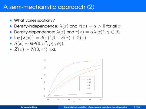
• What varies spatially?
• Density-independence: λ(x) and r(x) = α > 0 for all x.
• Density-dependence: λ(x) and r(x) = αλ(x)γ , γ ∈ R.
• log{λ(x)} = d(x)>β + S(x) + Z(x).• S(x) ∼ GP(0, σ2, ρ(·;φ)).• Z(x) ∼ N(0, τ 2) i.i.d.
0.0 0.2 0.4 0.6 0.8 1.0
0.0
0.2
0.4
0.6
0.8
1.0
p1
p 2 r = 0.1
r = 1.5
r = 2
r = 5
Figure 11: Relationship between ICT and MF prevalence.
Emanuele Giorgi Geostatistical modelling of prevalence data from two diagnostics 9 / 20

A semi-mechanistic approach (2)
• What varies spatially?
• Density-independence: λ(x) and r(x) = α > 0 for all x.
• Density-dependence: λ(x) and r(x) = αλ(x)γ , γ ∈ R.
• log{λ(x)} = d(x)>β + S(x) + Z(x).
• S(x) ∼ GP(0, σ2, ρ(·;φ)).• Z(x) ∼ N(0, τ 2) i.i.d.
0.0 0.2 0.4 0.6 0.8 1.0
0.0
0.2
0.4
0.6
0.8
1.0
p1
p 2 r = 0.1
r = 1.5
r = 2
r = 5
Figure 11: Relationship between ICT and MF prevalence.
Emanuele Giorgi Geostatistical modelling of prevalence data from two diagnostics 9 / 20

A semi-mechanistic approach (2)
• What varies spatially?
• Density-independence: λ(x) and r(x) = α > 0 for all x.
• Density-dependence: λ(x) and r(x) = αλ(x)γ , γ ∈ R.
• log{λ(x)} = d(x)>β + S(x) + Z(x).• S(x) ∼ GP(0, σ2, ρ(·;φ)).
• Z(x) ∼ N(0, τ 2) i.i.d.
0.0 0.2 0.4 0.6 0.8 1.0
0.0
0.2
0.4
0.6
0.8
1.0
p1
p 2 r = 0.1
r = 1.5
r = 2
r = 5
Figure 11: Relationship between ICT and MF prevalence.
Emanuele Giorgi Geostatistical modelling of prevalence data from two diagnostics 9 / 20

A semi-mechanistic approach (2)
• What varies spatially?
• Density-independence: λ(x) and r(x) = α > 0 for all x.
• Density-dependence: λ(x) and r(x) = αλ(x)γ , γ ∈ R.
• log{λ(x)} = d(x)>β + S(x) + Z(x).• S(x) ∼ GP(0, σ2, ρ(·;φ)).• Z(x) ∼ N(0, τ 2) i.i.d.
0.0 0.2 0.4 0.6 0.8 1.0
0.0
0.2
0.4
0.6
0.8
1.0
p1
p 2 r = 0.1
r = 1.5
r = 2
r = 5
Figure 11: Relationship between ICT and MF prevalence.
Emanuele Giorgi Geostatistical modelling of prevalence data from two diagnostics 9 / 20
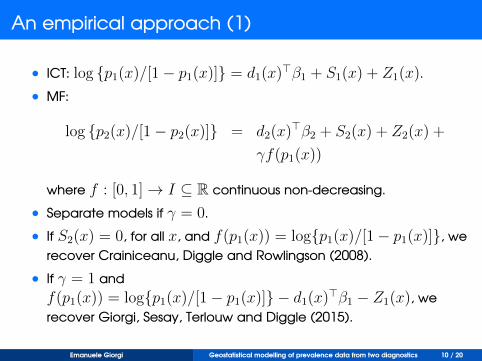
An empirical approach (1)
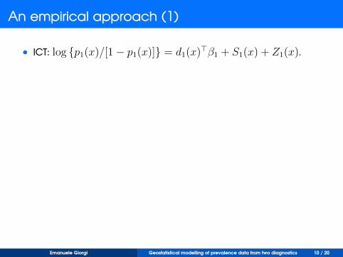
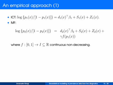
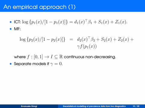
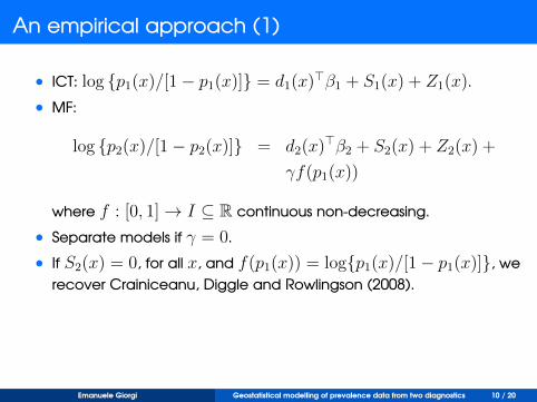
• ICT: log {p1(x)/[1− p1(x)]} = d1(x)>β1 + S1(x) + Z1(x).
• MF:
log {p2(x)/[1− p2(x)]} = d2(x)>β2 + S2(x) + Z2(x) +
γf(p1(x))
where f : [0, 1]→ I ⊆ R continuous non-decreasing.
• Separate models if γ = 0.
• If S2(x) = 0, for all x, and f(p1(x)) = log{p1(x)/[1− p1(x)]}, we
recover Crainiceanu, Diggle and Rowlingson (2008).
• If γ = 1 and
f(p1(x)) = log{p1(x)/[1− p1(x)]} − d1(x)>β1 − Z1(x), we
recover Giorgi, Sesay, Terlouw and Diggle (2015).
Emanuele Giorgi Geostatistical modelling of prevalence data from two diagnostics 10 / 20
An empirical approach (1)
• ICT: log {p1(x)/[1− p1(x)]} = d1(x)>β1 + S1(x) + Z1(x).
• MF:
log {p2(x)/[1− p2(x)]} = d2(x)>β2 + S2(x) + Z2(x) +
γf(p1(x))
where f : [0, 1]→ I ⊆ R continuous non-decreasing.
• Separate models if γ = 0.
• If S2(x) = 0, for all x, and f(p1(x)) = log{p1(x)/[1− p1(x)]}, we
recover Crainiceanu, Diggle and Rowlingson (2008).
• If γ = 1 and
f(p1(x)) = log{p1(x)/[1− p1(x)]} − d1(x)>β1 − Z1(x), we
recover Giorgi, Sesay, Terlouw and Diggle (2015).
Emanuele Giorgi Geostatistical modelling of prevalence data from two diagnostics 10 / 20
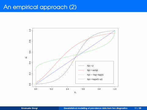
An empirical approach (2)
0.0 0.2 0.4 0.6 0.8 1.0
0.0
0.2
0.4
0.6
0.8
1.0
p1
p 2
f(p) = p
f(p) = sqrt(p)
f(p) = −log(−log(p))
f(p) = log(p/(1−p))
Emanuele Giorgi Geostatistical modelling of prevalence data from two diagnostics 11 / 20
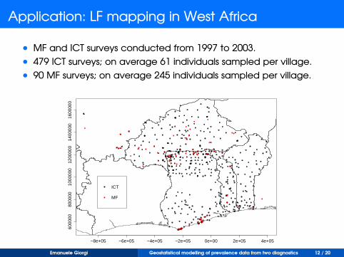
Application: LF mapping in West Africa
• MF and ICT surveys conducted from 1997 to 2003.
• 479 ICT surveys; on average 61 individuals sampled per village.
• 90 MF surveys; on average 245 individuals sampled per village.
−8e+05 −6e+05 −4e+05 −2e+05 0e+00 2e+05 4e+05
6000
0080
0000
1000
000
1200
000
1400
000
1600
000
ICT
MF
Emanuele Giorgi Geostatistical modelling of prevalence data from two diagnostics 12 / 20
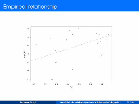
Empirical relationship
0.1 0.2 0.3 0.4 0.5 0.6 0.7
−7
−6
−5
−4
−3
−2
−1
p1
logi
t(p2)
Emanuele Giorgi Geostatistical modelling of prevalence data from two diagnostics 13 / 20
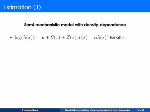
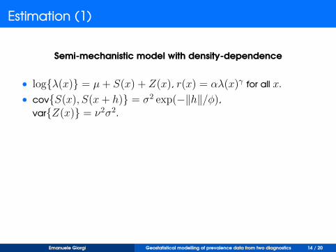
Estimation (1)
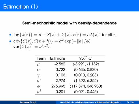
Semi-mechanistic model with density-dependence
• log{λ(x)} = µ+ S(x) + Z(x), r(x) = αλ(x)γ for all x.
• cov{S(x), S(x+ h)} = σ2 exp(−‖h‖/φ),var{Z(x)} = ν2σ2.
Term Estimate 95% CI
µ -2.562 (-3.991, -1.132)
α 0.722 (0.636, 0.820)
γ 0.106 (0.010, 0.203)
σ2 2.974 (1.392, 6.355)
φ 275.995 (117.374, 648.980)
ν2 0.201 (0.091, 0.445)
Emanuele Giorgi Geostatistical modelling of prevalence data from two diagnostics 14 / 20
Estimation (1)
Semi-mechanistic model with density-dependence
• log{λ(x)} = µ+ S(x) + Z(x), r(x) = αλ(x)γ for all x.
• cov{S(x), S(x+ h)} = σ2 exp(−‖h‖/φ),var{Z(x)} = ν2σ2.
Term Estimate 95% CI
µ -2.562 (-3.991, -1.132)
α 0.722 (0.636, 0.820)
γ 0.106 (0.010, 0.203)
σ2 2.974 (1.392, 6.355)
φ 275.995 (117.374, 648.980)
ν2 0.201 (0.091, 0.445)
Emanuele Giorgi Geostatistical modelling of prevalence data from two diagnostics 14 / 20
Estimation (2)
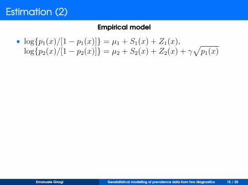
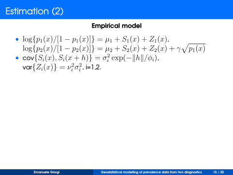
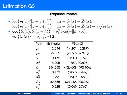
Empirical model
• log{p1(x)/[1− p1(x)]} = µ1 + S1(x) + Z1(x),log{p2(x)/[1− p2(x)]} = µ2 + S2(x) + Z2(x) + γ
√p1(x)
• cov{Si(x), Si(x+ h)} = σ2i exp(−‖h‖/φi),
var{Zi(x)} = ν2i σ2i , i=1,2.
Term Estimate 95% CI
µ1 -2.244 (-4.201, -0.287)
µ2 -3.055 (-3.763, -2.348)
γ 0.476 (0.200, 0.752)
σ21 4.205 (1.667, 10.608)
φ1 354.055 (126.608, 990.106)
ν21 0.172 (0.066, 0.449)
σ22 1.796 (0.909, 3.550)
φ2 82.555 (34.412, 198.052)
ν22 0.228 (0.069, 0.760)
Emanuele Giorgi Geostatistical modelling of prevalence data from two diagnostics 15 / 20
Estimation (2)
Empirical model
• log{p1(x)/[1− p1(x)]} = µ1 + S1(x) + Z1(x),log{p2(x)/[1− p2(x)]} = µ2 + S2(x) + Z2(x) + γ
√p1(x)
• cov{Si(x), Si(x+ h)} = σ2i exp(−‖h‖/φi),
var{Zi(x)} = ν2i σ2i , i=1,2.
Term Estimate 95% CI
µ1 -2.244 (-4.201, -0.287)
µ2 -3.055 (-3.763, -2.348)
γ 0.476 (0.200, 0.752)
σ21 4.205 (1.667, 10.608)
φ1 354.055 (126.608, 990.106)
ν21 0.172 (0.066, 0.449)
σ22 1.796 (0.909, 3.550)
φ2 82.555 (34.412, 198.052)
ν22 0.228 (0.069, 0.760)
Emanuele Giorgi Geostatistical modelling of prevalence data from two diagnostics 15 / 20
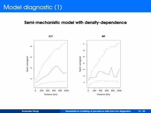
Model diagnostic (1)
Semi-mechanistic model with density-dependence
0 200 400 600 800 1000
24
68
ICT
Distance (km)
Sem
i−va
riogr
am
0 200 400 600 800 1000
12
34
56
7
MF
Distance (km)
Sem
i−va
riogr
am
Emanuele Giorgi Geostatistical modelling of prevalence data from two diagnostics 16 / 20
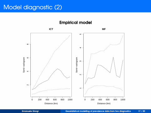
Model diagnostic (2)
Empirical model
0 200 400 600 800 1000
24
68
ICT
Distance (km)
Sem
i−va
riogr
am
0 200 400 600 800 1000
12
34
5
MF
Distance (km)
Sem
i−va
riogr
am
Emanuele Giorgi Geostatistical modelling of prevalence data from two diagnostics 17 / 20
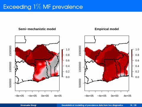
Exceeding 1% MF prevalence
−8e+05 −4e+05 0e+00 4e+05
5000
0010
0000
015
0000
0
Semi−mechanistic model
0.0
0.2
0.4
0.6
0.8
1.0
−8e+05 −4e+05 0e+00 4e+05
5000
0010
0000
015
0000
0
Empirical model
0.0
0.2
0.4
0.6
0.8
1.0
Emanuele Giorgi Geostatistical modelling of prevalence data from two diagnostics 18 / 20

Discussion
• Which model is the best with respect to the scientific knowledge?
• Simulation study: empirical model provides robust inferences
against the misspecification of f .
• Simulation study: misspecification of the model may still yield
accurate point predictions but actual coverage of CI may be very
different from the nominal.
Thank you for your attention!
Emanuele Giorgi Geostatistical modelling of prevalence data from two diagnostics 19 / 20
Bibliography
1 M. A. Irvine, S. M. Njenga, S. Gunawardena, C. N. Wamae, J.
Cano, S. J. Brooker, and T. D. Hollingsworth. Understanding therelationship between prevalence of microfilariae andantigenaemia using a model of lymphatic filariasis infection. Trans
R Soc Trop Med Hyg (2016) 110(5): 317 doi:10.1093/trstmh/trw024
2 C. Crainiceanu, P.J. Diggle, and B.S. Rowlingson. Bivariatemodelling and prediction of spatial variation in Loa loaprevalence in tropical Africa (with Discussion). (2008) Journal of
the American Statistical Association, 103, 21-43.
3 E. Giorgi, S.S. Sesay, D.J. Terlouw and P.J., Diggle. Combining datafrom multiple spatially referenced prevalence surveys usinggeneralized linear geostatistical models. (2015) Journal of the
Royal Statistical Society A 178, 445-464.
Emanuele Giorgi Geostatistical modelling of prevalence data from two diagnostics 20 / 20