Embed Size (px)
Citation preview

Geospatial Data in R
Geospatial Datain RAnd Beyond!
Barry [email protected]
School of Health and Medicine,Lancaster University

Spatial Data in R
Historicalperspective

Before R
The S Language (Chambers, Becker, Wilks) Born 1976 Released 1984 Reborn 1988 (The New S Language)
S-Plus Commercialised version, 1988
Image from amazon.com
points, polygon, lines
“Roll your own” maps
plot(xy,asp=1)
polygon(xy,col=...)
points(xy,pch=...)
lines(xy,lwd=2,...)
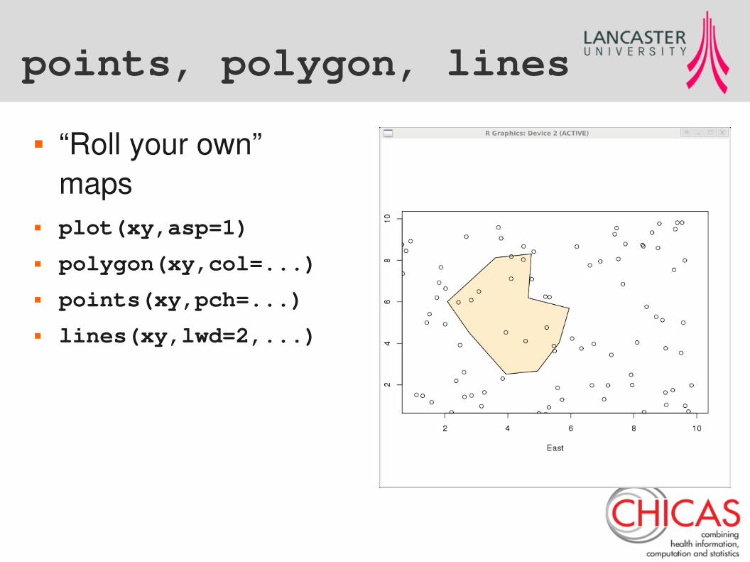
First Maps
The map package: Becker and Wilks library(maps);map()
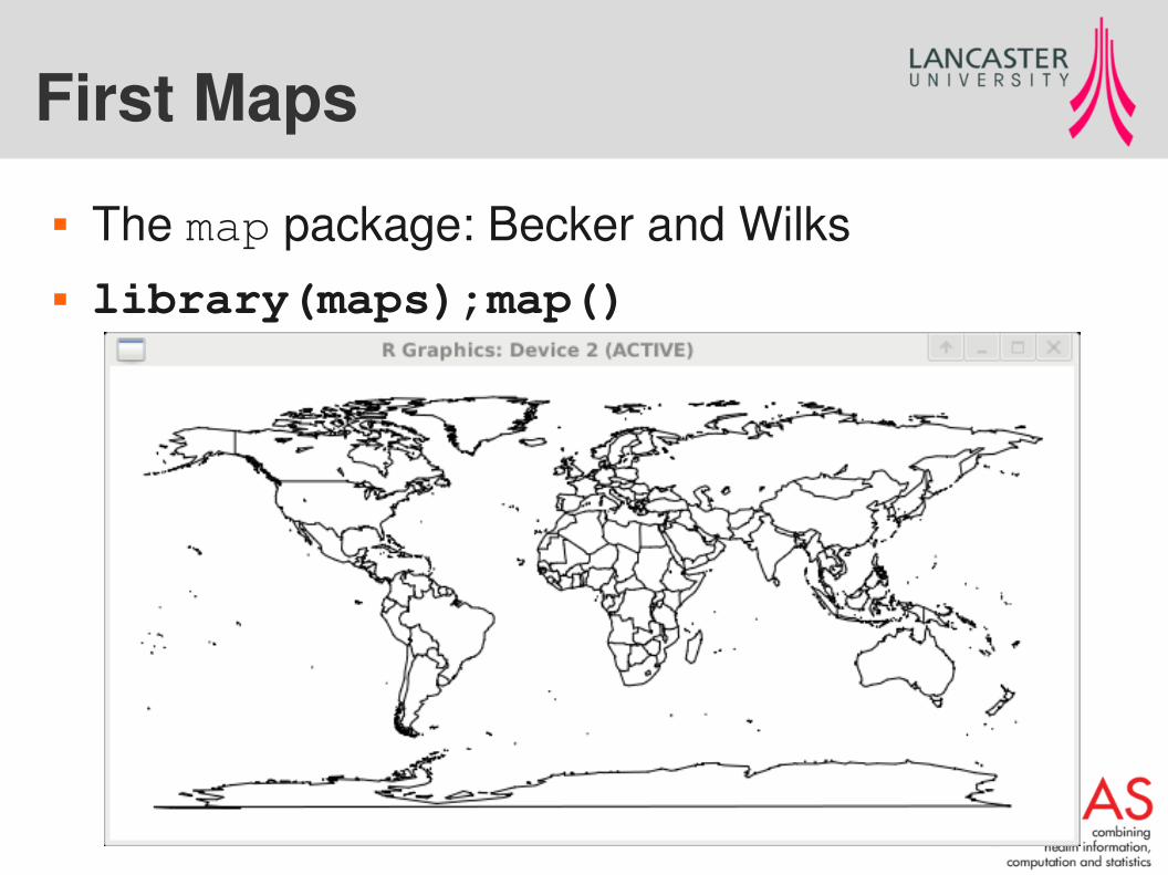
map(database,regions,...)
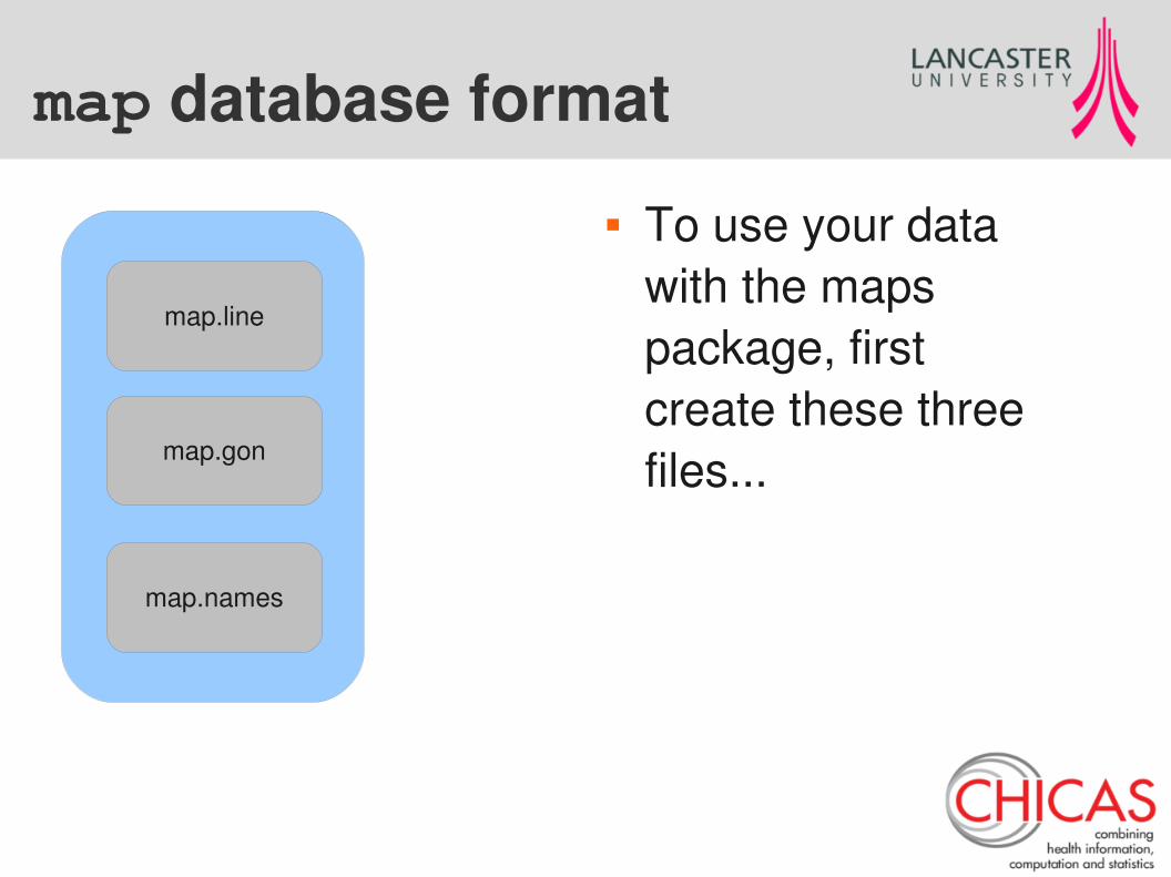
map database format
map.line
map.gon
map.names
To use your data with the maps package, first create these three files...
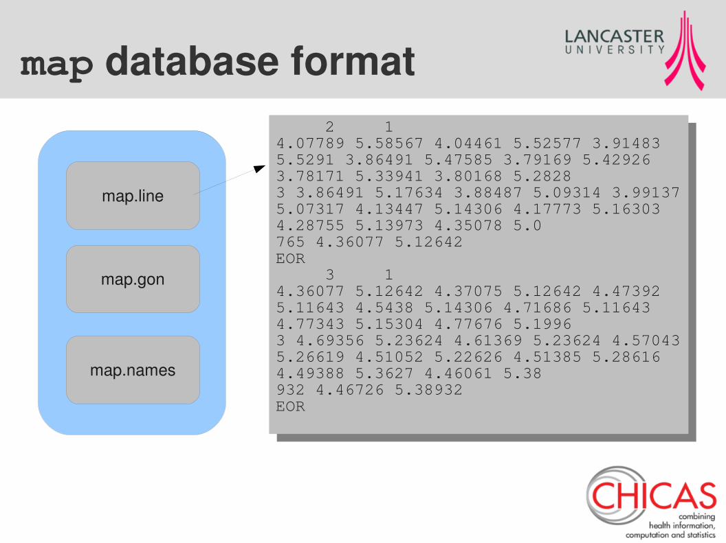
map database format
map.line
map.gon
map.names
2 14.07789 5.58567 4.04461 5.52577 3.91483 5.5291 3.86491 5.47585 3.79169 5.42926 3.78171 5.33941 3.80168 5.28283 3.86491 5.17634 3.88487 5.09314 3.99137 5.07317 4.13447 5.14306 4.17773 5.16303 4.28755 5.13973 4.35078 5.0765 4.36077 5.12642EOR 3 14.36077 5.12642 4.37075 5.12642 4.47392 5.11643 4.5438 5.14306 4.71686 5.11643 4.77343 5.15304 4.77676 5.19963 4.69356 5.23624 4.61369 5.23624 4.57043 5.26619 4.51052 5.22626 4.51385 5.28616 4.49388 5.3627 4.46061 5.38932 4.46726 5.38932EOR
2 14.07789 5.58567 4.04461 5.52577 3.91483 5.5291 3.86491 5.47585 3.79169 5.42926 3.78171 5.33941 3.80168 5.28283 3.86491 5.17634 3.88487 5.09314 3.99137 5.07317 4.13447 5.14306 4.17773 5.16303 4.28755 5.13973 4.35078 5.0765 4.36077 5.12642EOR 3 14.36077 5.12642 4.37075 5.12642 4.47392 5.11643 4.5438 5.14306 4.71686 5.11643 4.77343 5.15304 4.77676 5.19963 4.69356 5.23624 4.61369 5.23624 4.57043 5.26619 4.51052 5.22626 4.51385 5.28616 4.49388 5.3627 4.46061 5.38932 4.46726 5.38932EOR
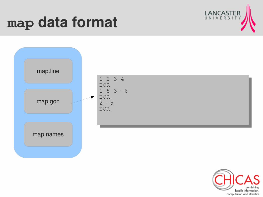
map data format
map.line
map.gon
map.names
1 2 3 4EOR1 5 3 -6EOR2 -5EOR
1 2 3 4EOR1 5 3 -6EOR2 -5EOR
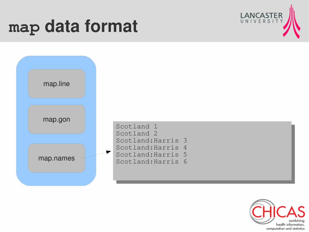
map data format
map.line
map.gon
map.names
Scotland 1Scotland 2Scotland:Harris 3Scotland:Harris 4Scotland:Harris 5Scotland:Harris 6
Scotland 1Scotland 2Scotland:Harris 3Scotland:Harris 4Scotland:Harris 5Scotland:Harris 6
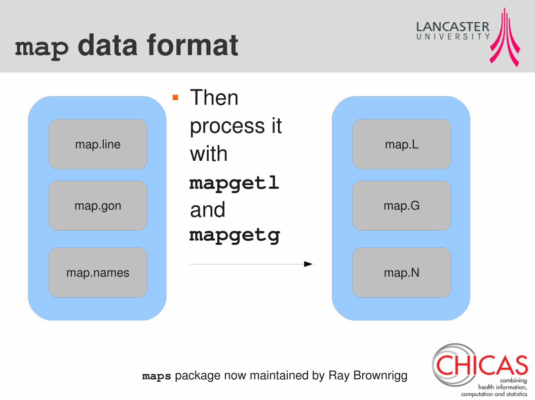
map data format
map.line
map.gon
map.names
map.L
map.G
map.N
Then process it with mapgetl and mapgetg
maps package now maintained by Ray Brownrigg
New Millennium
GIS spreading Many more map file formats (shapefile, 1998) Maps on the web (UMN Mapserver, mid-90s) Spatial Data Standards:
R didn't get left behind!
Perceived need for better maps Better spatial data handling Assorted little projects (my Rmap!)
Vector data - the sp classes
2004 : A Geospatial Odyssey More than just polygons!
Classes for points, lines, grids of points and polygons.
Geometry + Data for each feature Bivand, Pebesma, Gomez-Rubio “Simple Features” OGC spec
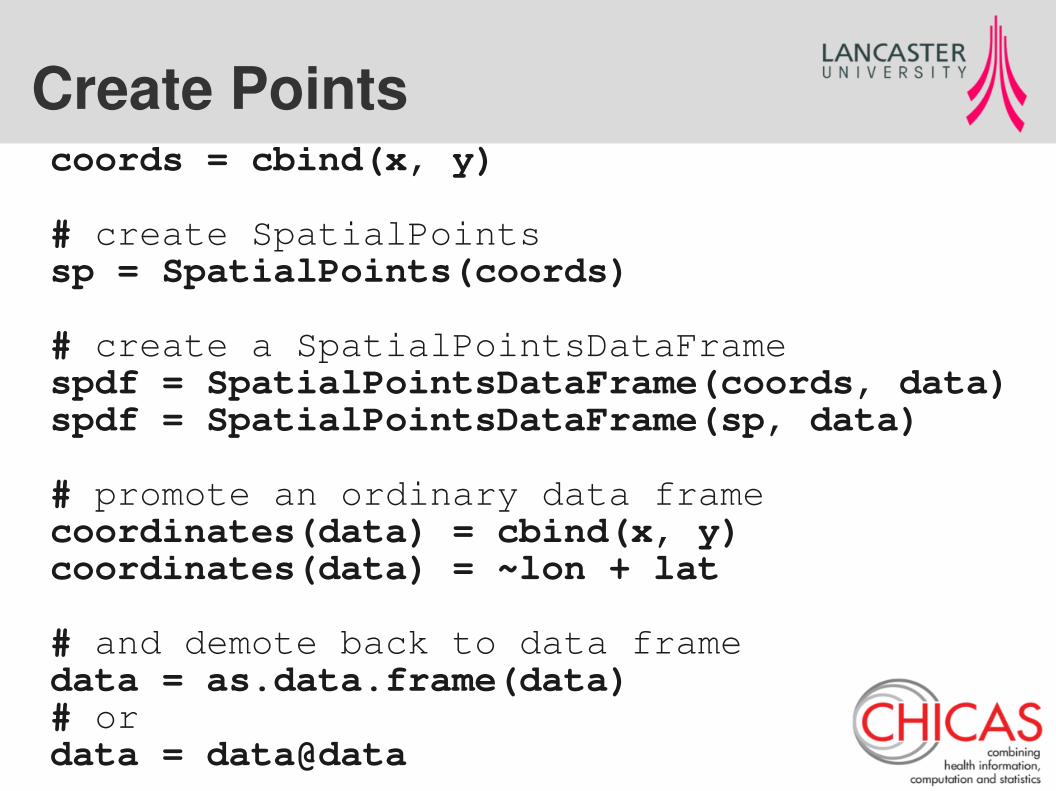
Create Points coords = cbind(x, y)
# create SpatialPointssp = SpatialPoints(coords)
# create a SpatialPointsDataFramespdf = SpatialPointsDataFrame(coords, data)spdf = SpatialPointsDataFrame(sp, data)
# promote an ordinary data framecoordinates(data) = cbind(x, y)coordinates(data) = ~lon + lat
# and demote back to data framedata = as.data.frame(data)# ordata = data@data
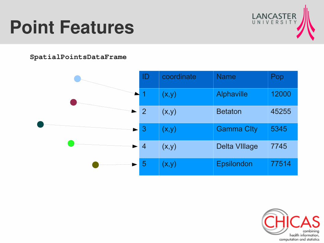
Point Features
ID coordinate Name Pop
1 (x,y) Alphaville 12000
2 (x,y) Betaton 45255
3 (x,y) Gamma CIty 5345
4 (x,y) Delta VIllage 7745
5 (x,y) Epsilondon 77514
SpatialPointsDataFrame
Manipulation
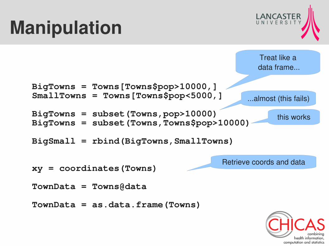
BigTowns = Towns[Towns$pop>10000,]SmallTowns = Towns[Towns$pop<5000,]
BigTowns = subset(Towns,pop>10000)BigTowns = subset(Towns,Towns$pop>10000)
BigSmall = rbind(BigTowns,SmallTowns)
xy = coordinates(Towns)
TownData = Towns@data
TownData = as.data.frame(Towns)
Treat like a data frame...
...almost (this fails)
Retrieve coords and data
this works
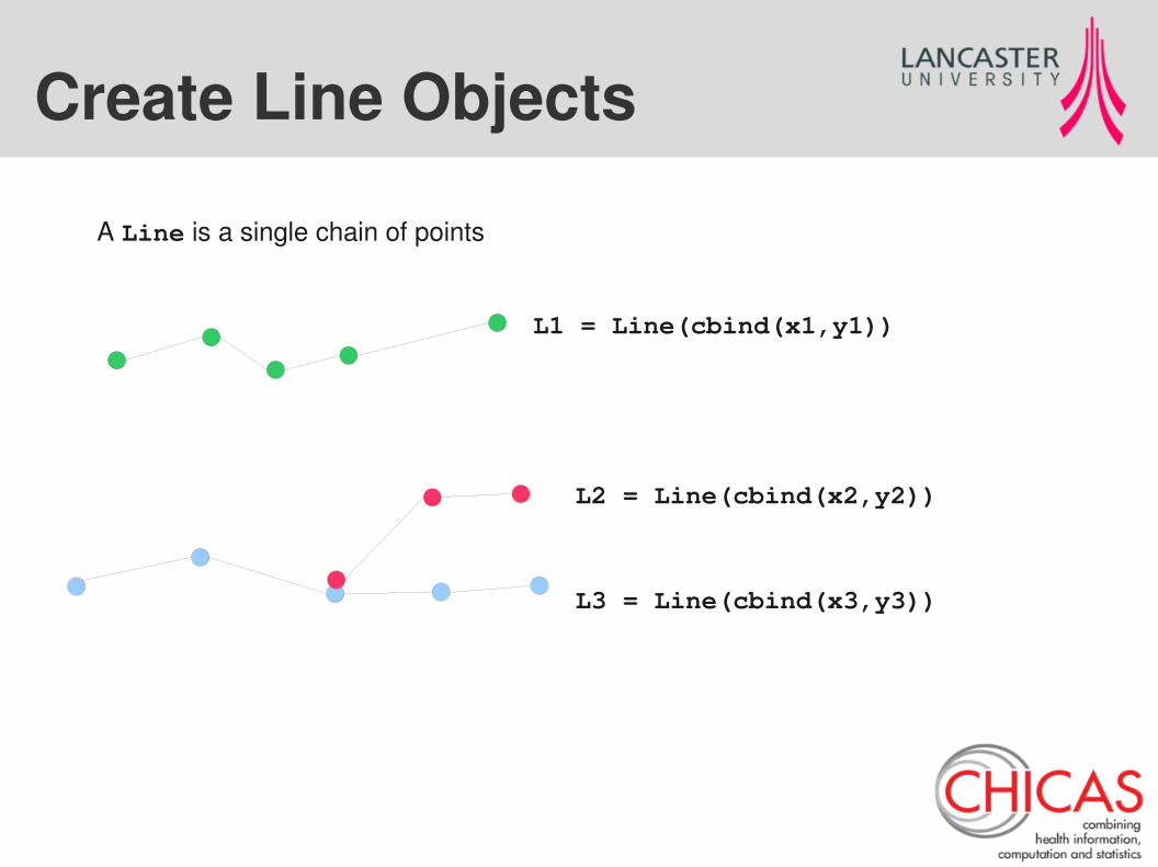
Create Line Objects
L2 = Line(cbind(x2,y2))
L3 = Line(cbind(x3,y3))
L1 = Line(cbind(x1,y1))
A Line is a single chain of points
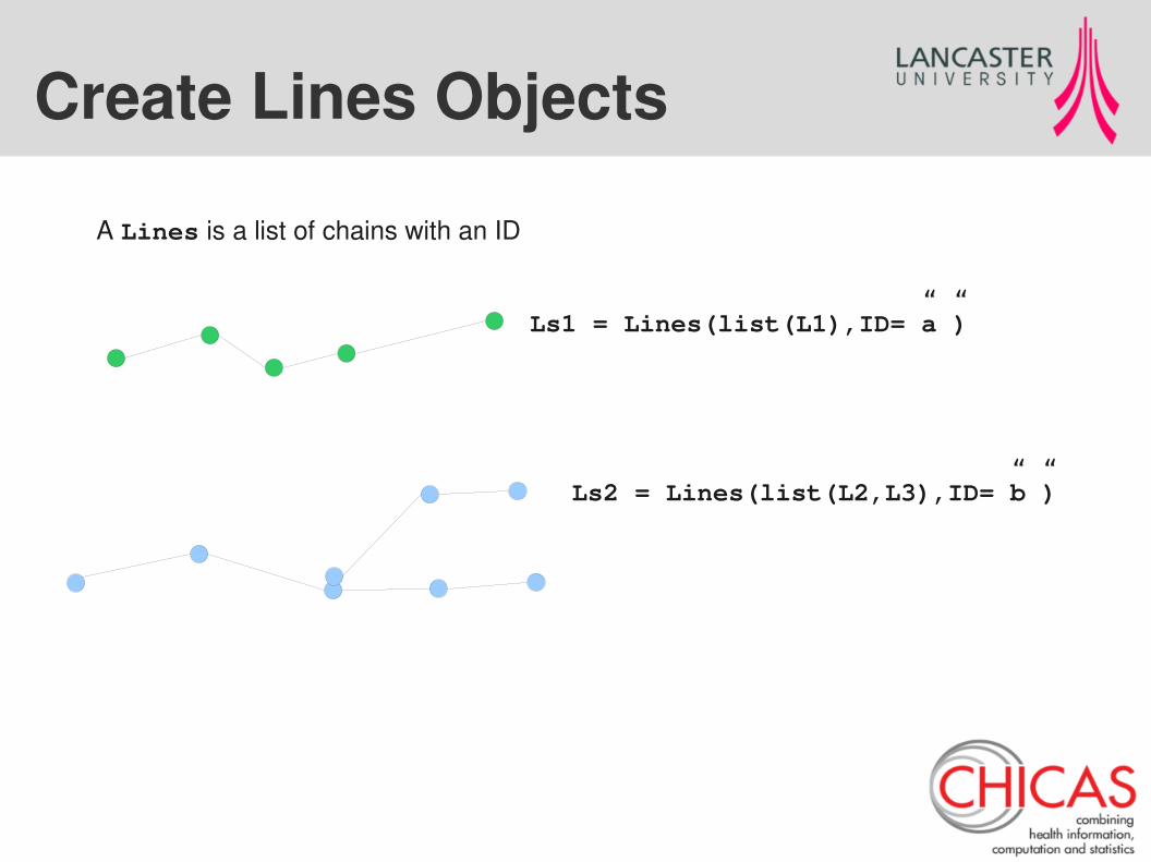
Create Lines Objects
Ls2 = Lines(list(L2,L3),ID=”b”)
Ls1 = Lines(list(L1),ID=”a”)
A Lines is a list of chains with an ID
Create SpatialLines Object
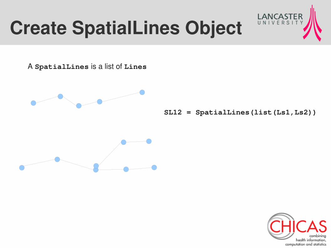
SL12 = SpatialLines(list(Ls1,Ls2))
A SpatialLines is a list of Lines
Create SpatialLinesDataFrame
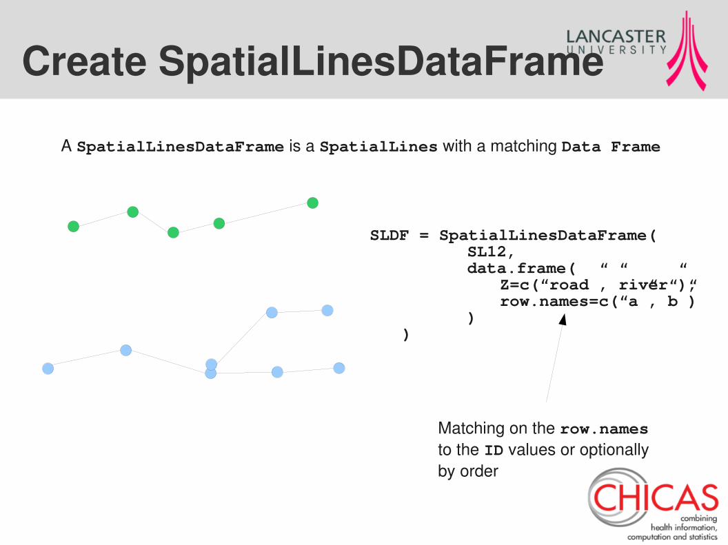
A SpatialLinesDataFrame is a SpatialLines with a matching Data Frame
SLDF = SpatialLinesDataFrame( SL12, data.frame(
Z=c(“road”,”river”),row.names=c(“a”,”b”)
))
Matching on the row.namesto the ID values or optionallyby order
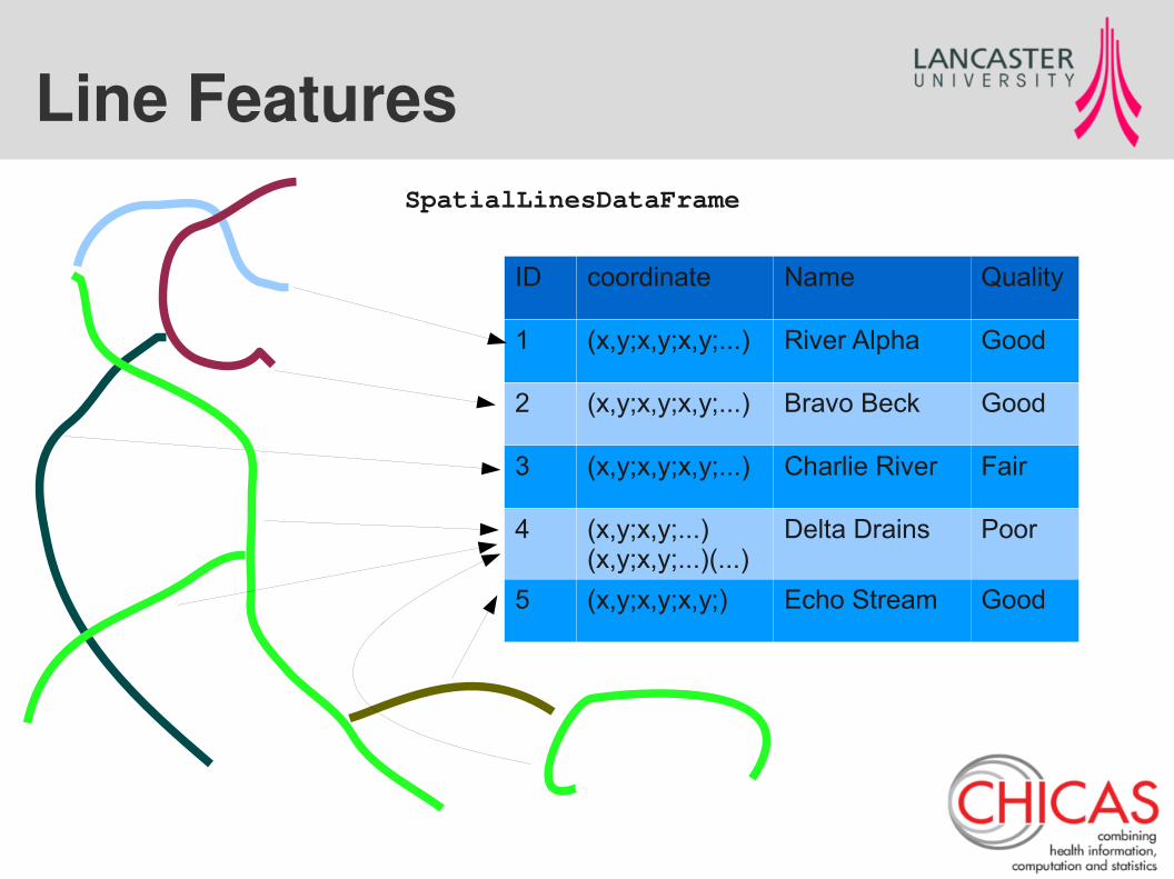
Line Features
ID coordinate Name Quality
1 (x,y;x,y;x,y;...) River Alpha Good
2 (x,y;x,y;x,y;...) Bravo Beck Good
3 (x,y;x,y;x,y;...) Charlie River Fair
4 (x,y;x,y;...)(x,y;x,y;...)(...)
Delta Drains Poor
5 (x,y;x,y;x,y;) Echo Stream Good
SpatialLinesDataFrame
Polygons
Now it starts to get complicated

Single Ring Feature
Make sure your coordinates connect:
c1 = cbind(x1,y1)r1 = rbind(c1,c1[1,])
A Polygon is a single ring
P1 = Polygon(r1)
A Polygons is a list of Polygon objects with an ID
Ps1 = Polygons(list(P1,ID=”a”))

Double Ring Feature
Make sure your coordinates connect:
c2a = cbind(x2a,y2a)r2a = rbind(c2a,c2a[1,])c2b = cbind(x2b,y2b)r2b = rbind(c2b,c2b[1,])
Make two single rings:
P2a = Polygon(r2a)P2b = Polygon(r2b)
Make a Polygons object with two rings
Ps2 = Polygons(list(P2a,P2b),ID=”b”))

Feature with hole
hc = cbind(xh,yh)rh = rbind(hc,hc[1,])
Make a holey Polygon:
H1 = Polygon(rh, hole=TRUE)
Make a Polygons object with two rings, one the hole
Ps3 = Polygons(list(P3,H1),ID=”c”))
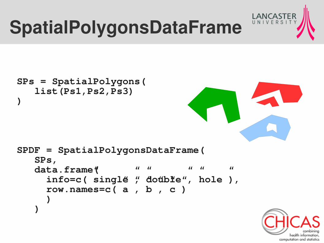
SpatialPolygonsDataFrame
SPs = SpatialPolygons( list(Ps1,Ps2,Ps3))
SPDF = SpatialPolygonsDataFrame( SPs, data.frame( info=c(”single”,”double”,”hole”), row.names=c(”a”,”b”,”c”) ) )
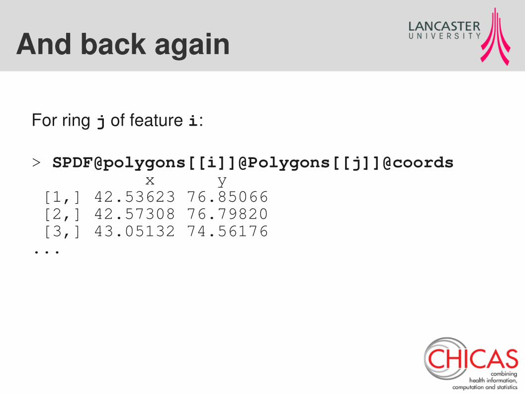
And back again
For ring j of feature i:
> SPDF@polygons[[i]]@Polygons[[j]]@coords x y [1,] 42.53623 76.85066 [2,] 42.57308 76.79820 [3,] 43.05132 74.56176...
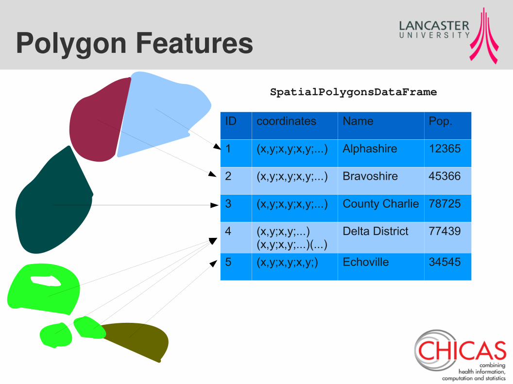
Polygon Features
ID coordinates Name Pop.
1 (x,y;x,y;x,y;...) Alphashire 12365
2 (x,y;x,y;x,y;...) Bravoshire 45366
3 (x,y;x,y;x,y;...) County Charlie 78725
4 (x,y;x,y;...)(x,y;x,y;...)(...)
Delta District 77439
5 (x,y;x,y;x,y;) Echoville 34545
SpatialPolygonsDataFrame
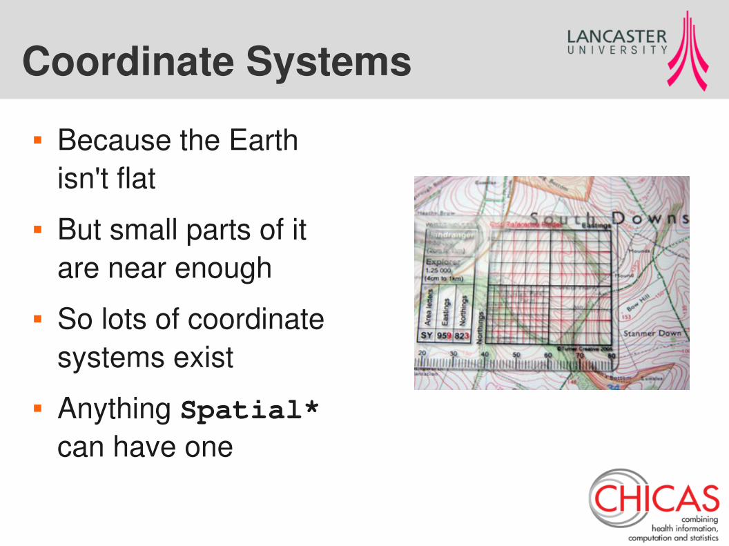
Coordinate Systems
Because the Earth isn't flat
But small parts of it are near enough
So lots of coordinate systems exist
Anything Spatial* can have one
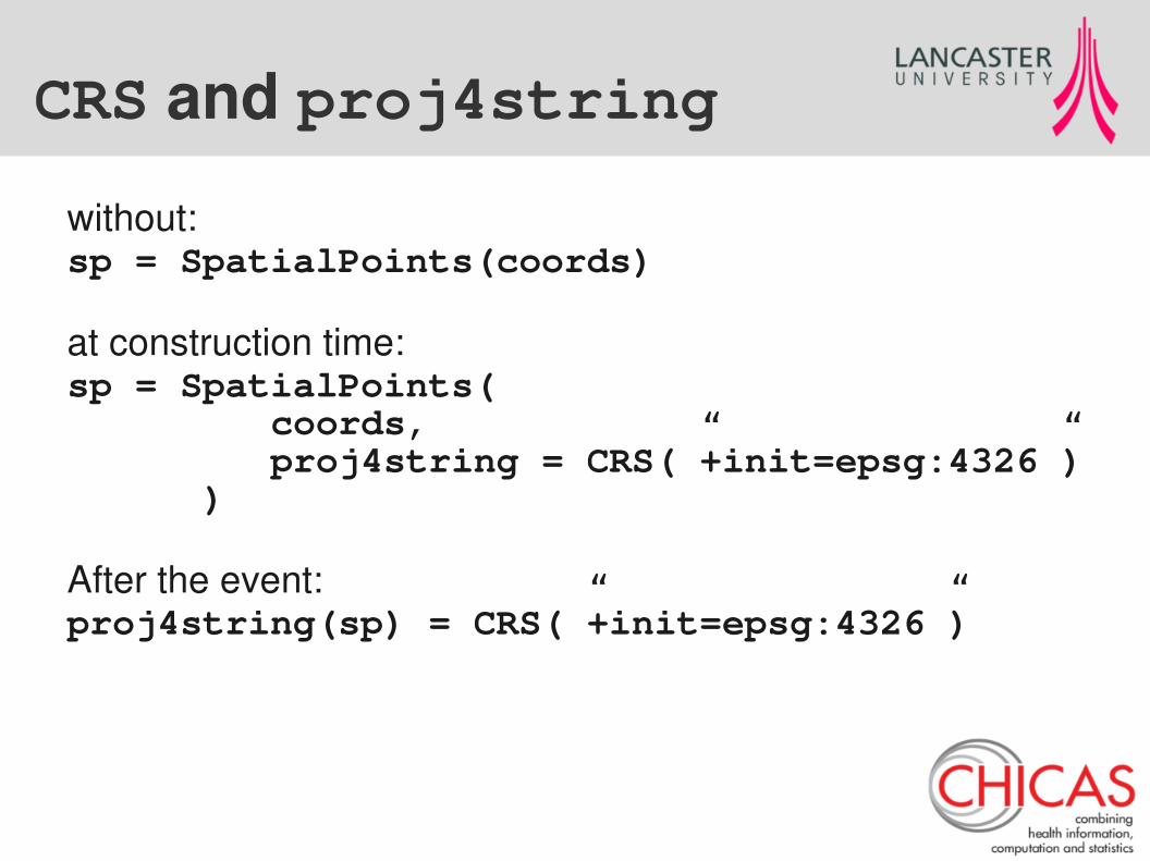
CRS and proj4string
without:sp = SpatialPoints(coords)
at construction time:sp = SpatialPoints( coords, proj4string = CRS(”+init=epsg:4326”) )
After the event:proj4string(sp) = CRS(”+init=epsg:4326”)
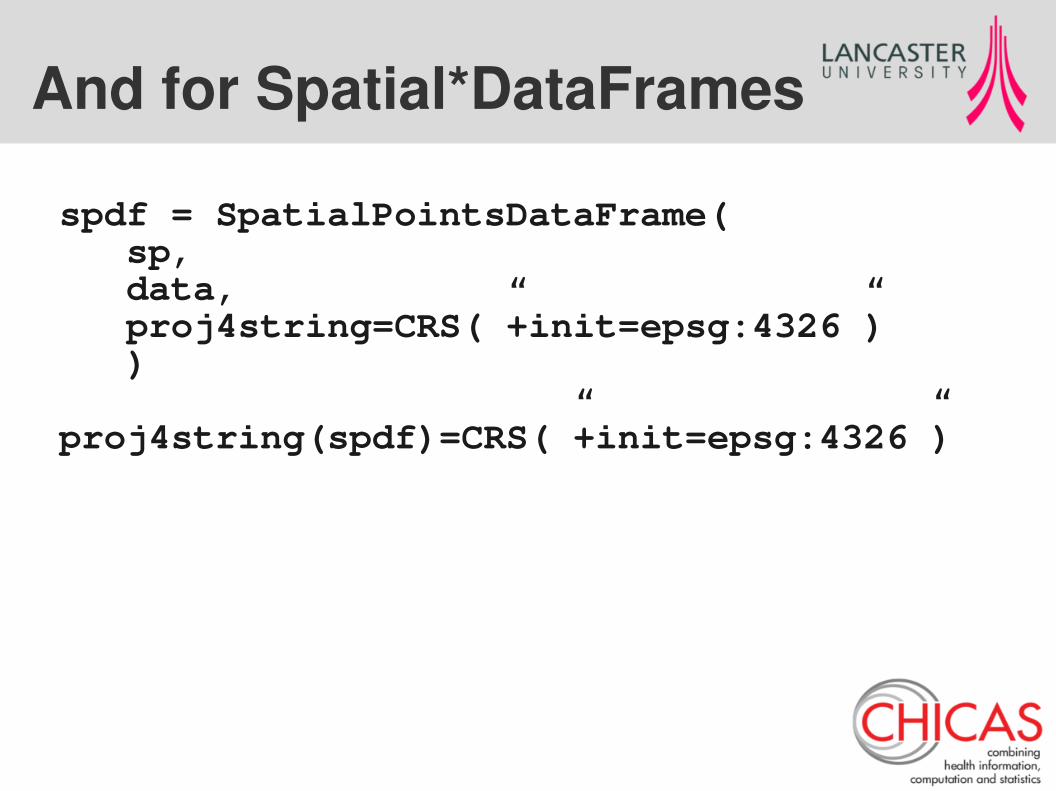
And for Spatial*DataFrames
spdf = SpatialPointsDataFrame( sp, data, proj4string=CRS(”+init=epsg:4326”) )
proj4string(spdf)=CRS(”+init=epsg:4326”)
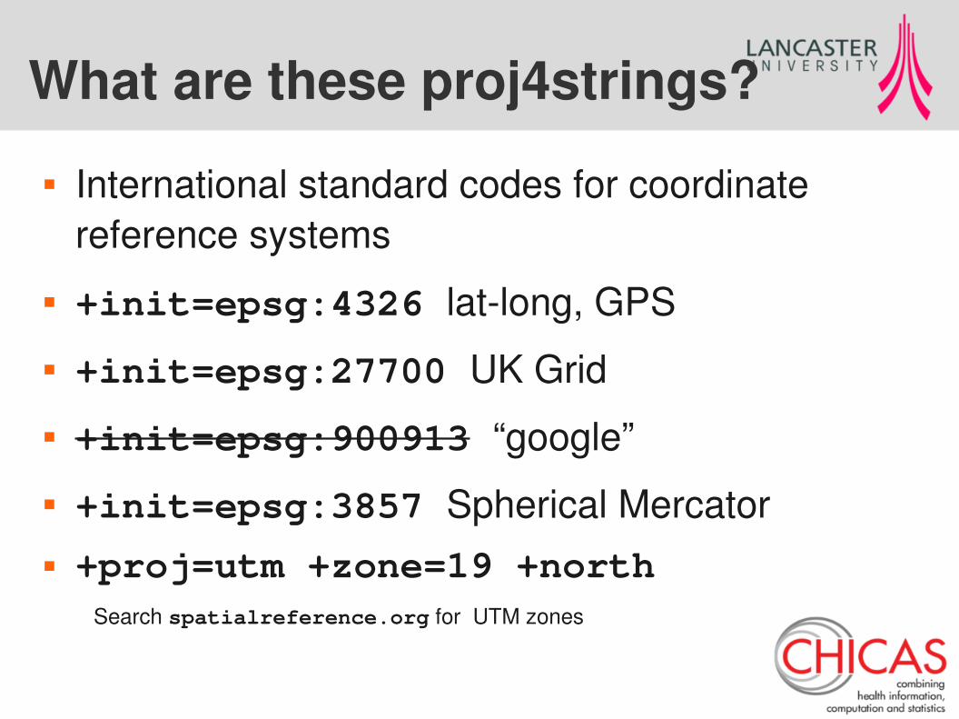
What are these proj4strings?
International standard codes for coordinate reference systems
+init=epsg:4326 lat-long, GPS +init=epsg:27700 UK Grid +init=epsg:900913 “google” +init=epsg:3857 Spherical Mercator +proj=utm +zone=19 +north
Search spatialreference.org for UTM zones
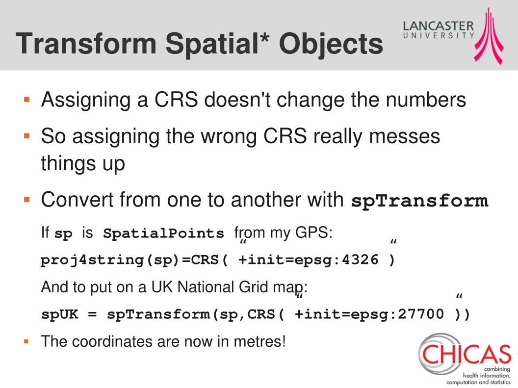
Transform Spatial* Objects
Assigning a CRS doesn't change the numbers So assigning the wrong CRS really messes
things up Convert from one to another with spTransform
If sp is SpatialPoints from my GPS:
proj4string(sp)=CRS(”+init=epsg:4326”)
And to put on a UK National Grid map:
spUK = spTransform(sp,CRS(”+init=epsg:27700”))
The coordinates are now in metres!
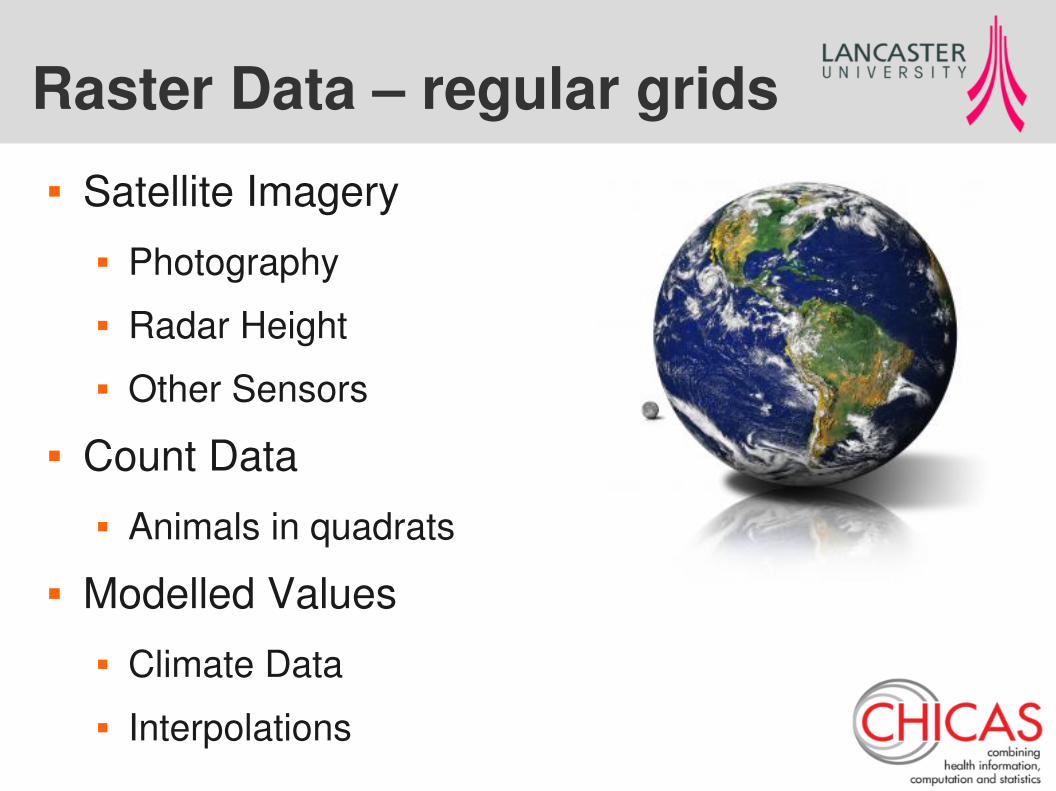
Raster Data – regular grids Satellite Imagery
Photography Radar Height Other Sensors
Count Data Animals in quadrats
Modelled Values Climate Data Interpolations
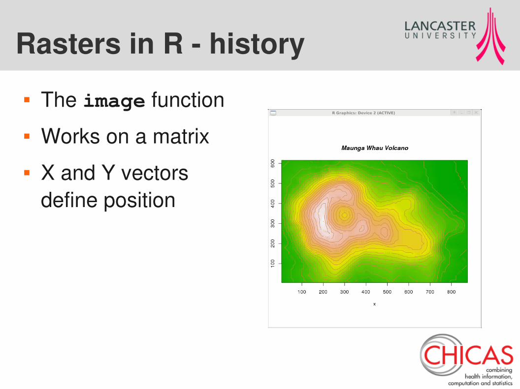
Rasters in R - history
The image function Works on a matrix X and Y vectors
define position
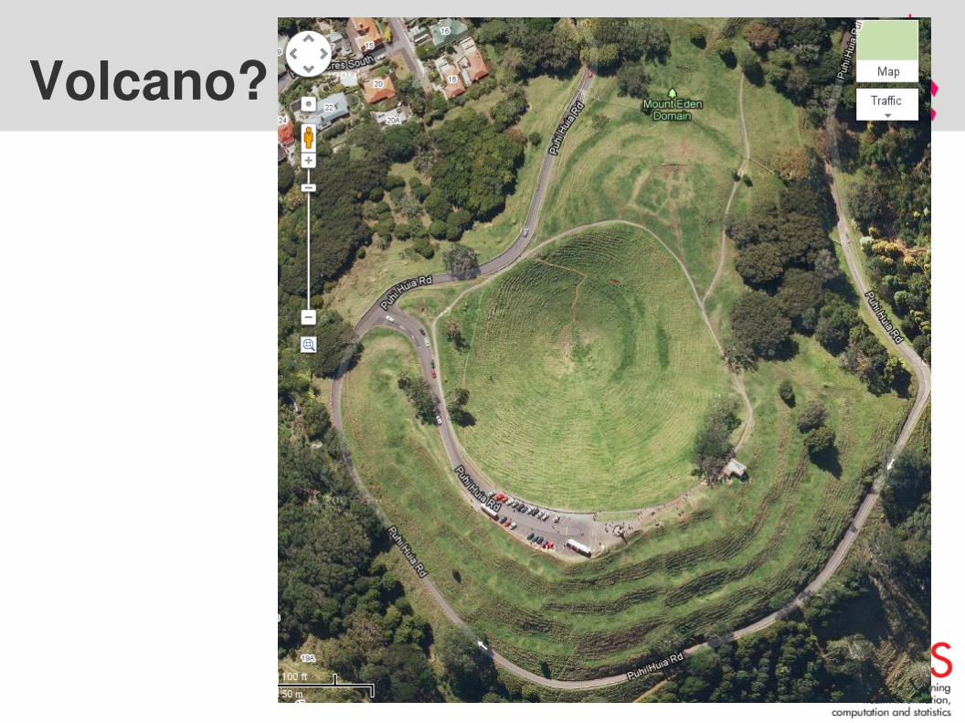
Volcano?
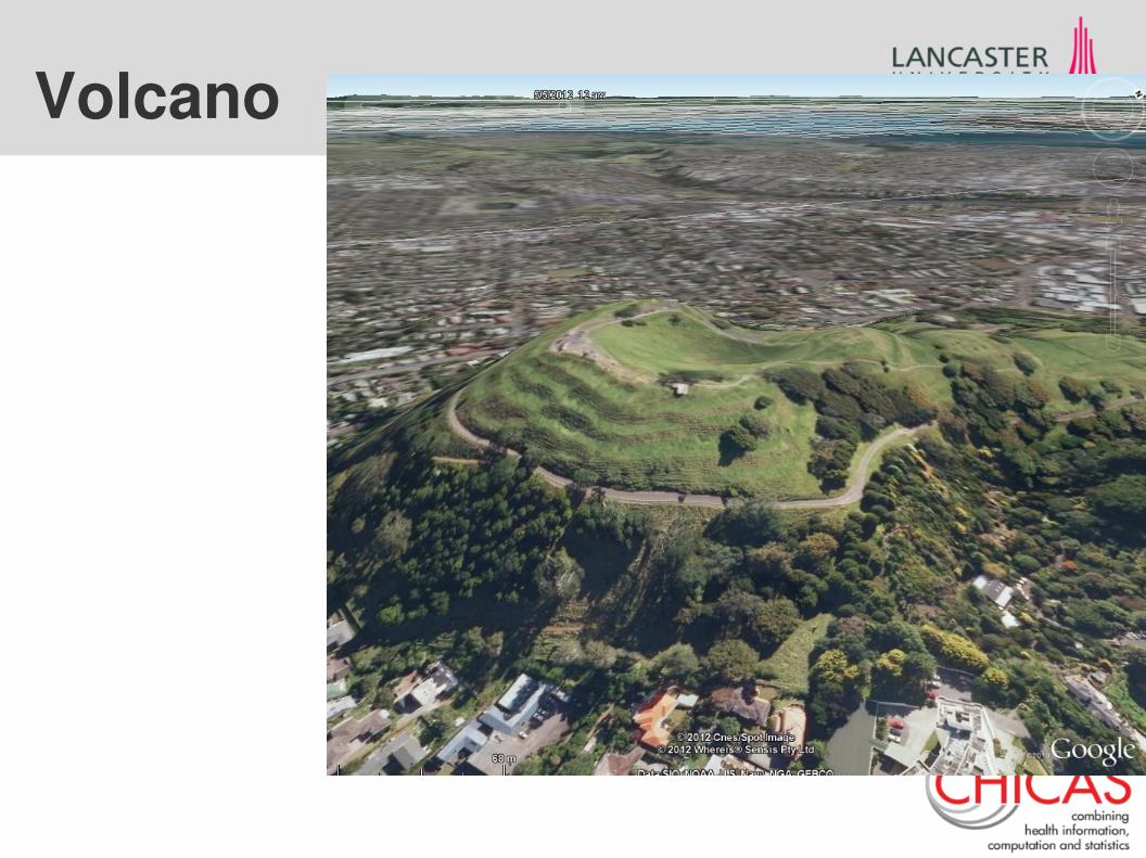
Volcano
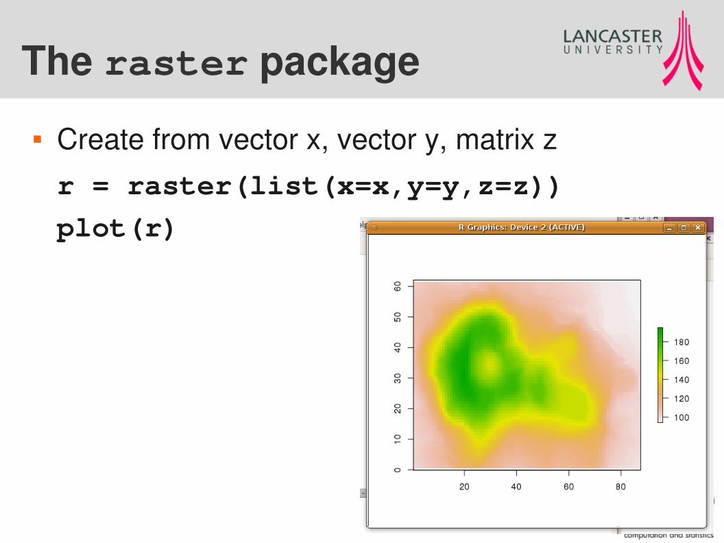
The raster package
Create from vector x, vector y, matrix zr = raster(list(x=x,y=y,z=z))
plot(r)
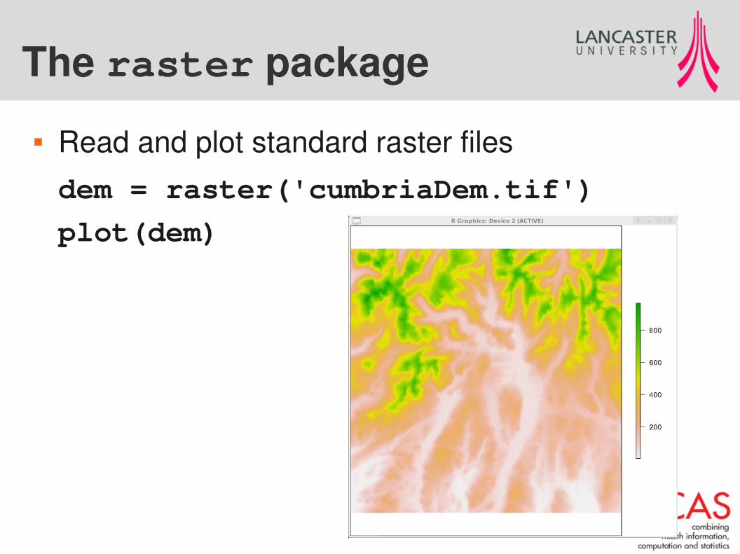
The raster package
Read and plot standard raster filesdem = raster('cumbriaDem.tif')
plot(dem)
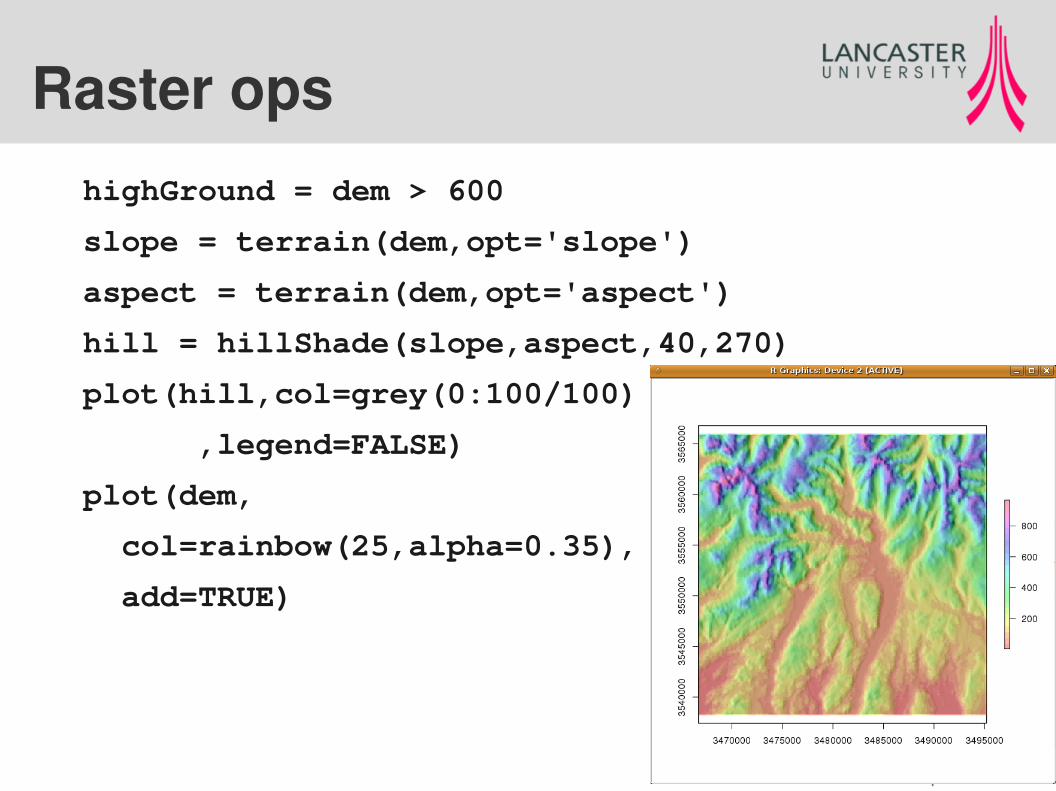
Raster opshighGround = dem > 600
slope = terrain(dem,opt='slope')
aspect = terrain(dem,opt='aspect')
hill = hillShade(slope,aspect,40,270)
plot(hill,col=grey(0:100/100)
,legend=FALSE)
plot(dem,
col=rainbow(25,alpha=0.35),
add=TRUE)
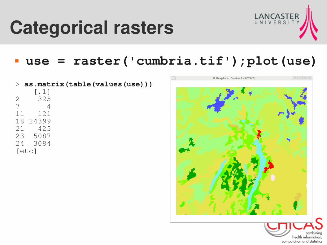
Categorical rasters use = raster('cumbria.tif');plot(use)
> as.matrix(table(values(use))) [,1]2 3257 411 12118 2439921 42523 508724 3084[etc]
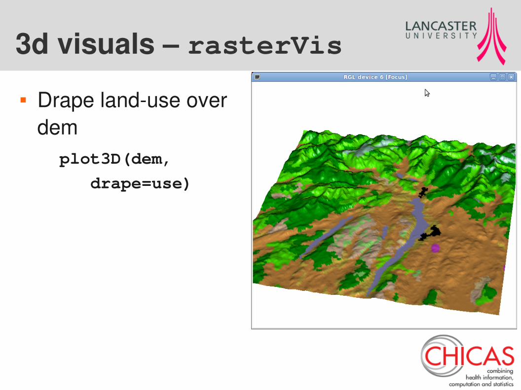
3d visuals – rasterVis
Drape land-use over dem
plot3D(dem,
drape=use)
Projections and CRS
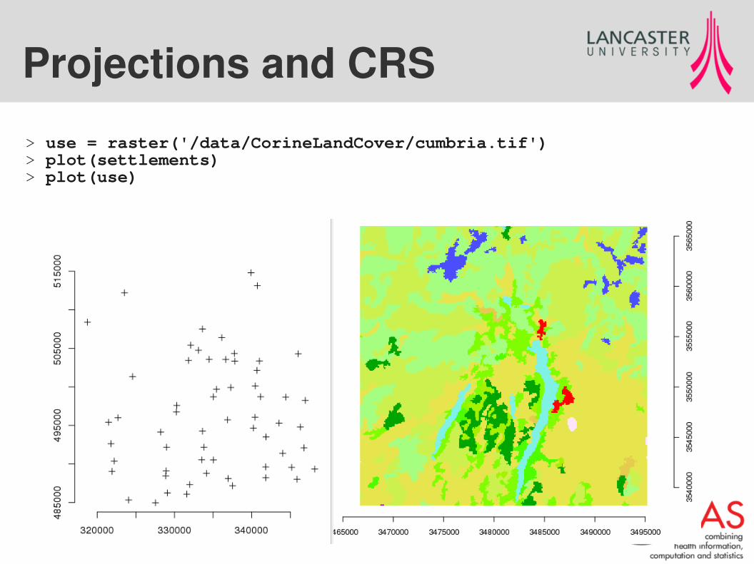
> use = raster('/data/CorineLandCover/cumbria.tif')> plot(settlements)> plot(use)
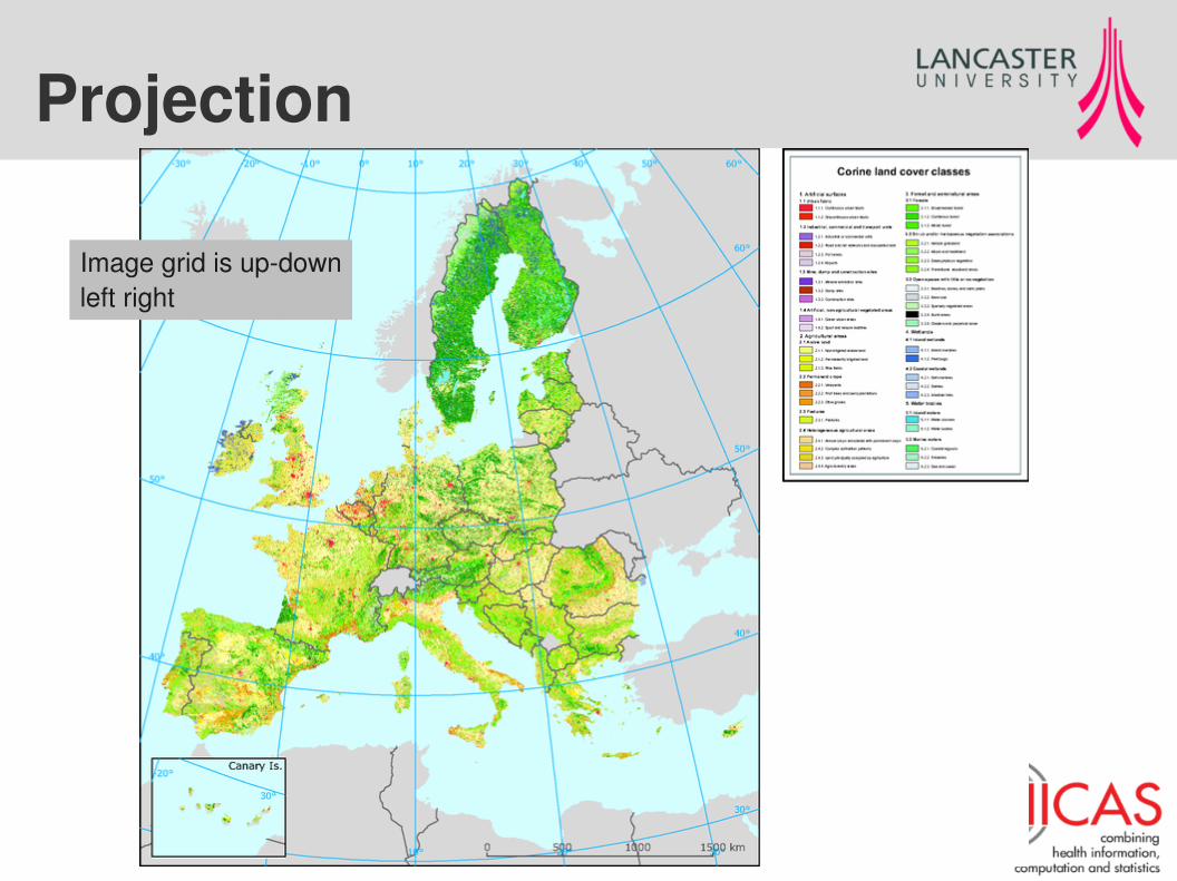
Projection
Image grid is up-downleft right
Projections
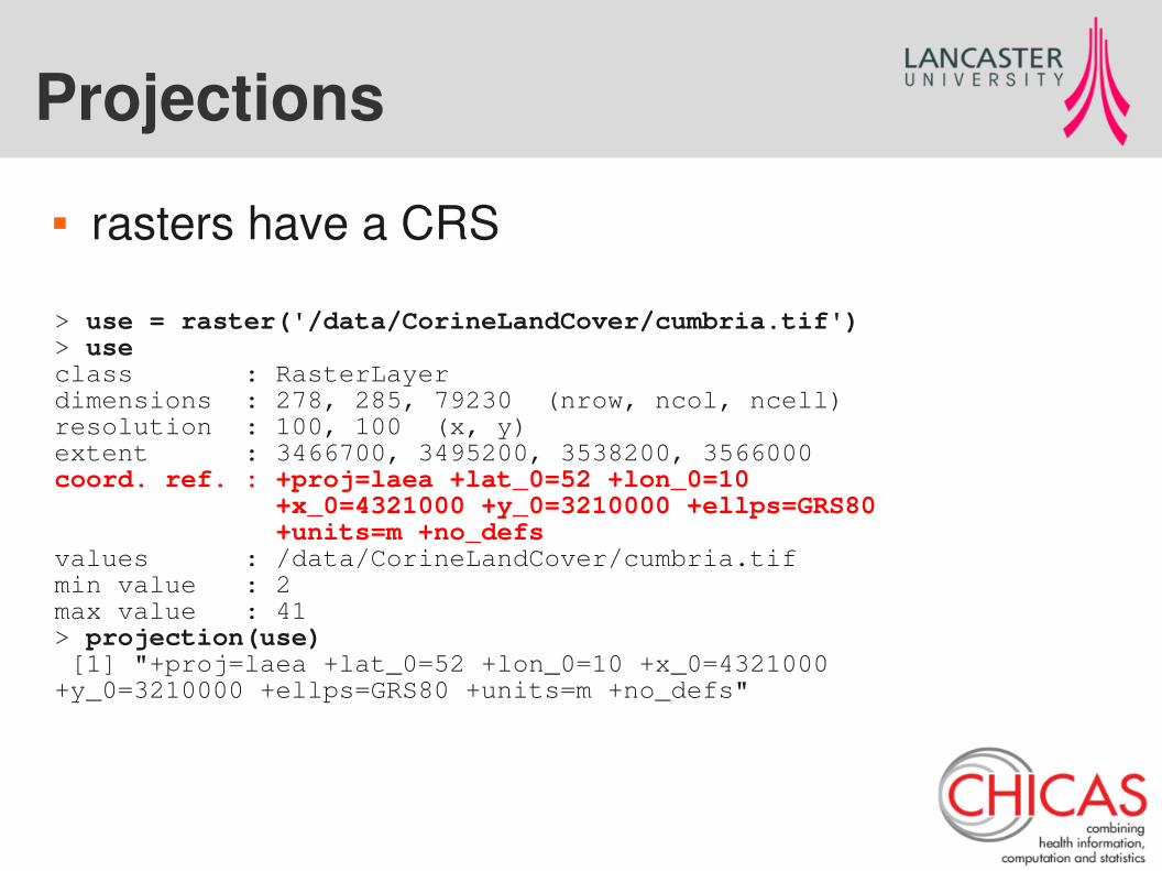
rasters have a CRS
> use = raster('/data/CorineLandCover/cumbria.tif')> useclass : RasterLayer dimensions : 278, 285, 79230 (nrow, ncol, ncell)resolution : 100, 100 (x, y)extent : 3466700, 3495200, 3538200, 3566000 coord. ref. : +proj=laea +lat_0=52 +lon_0=10 +x_0=4321000 +y_0=3210000 +ellps=GRS80 +units=m +no_defs values : /data/CorineLandCover/cumbria.tif min value : 2 max value : 41> projection(use) [1] "+proj=laea +lat_0=52 +lon_0=10 +x_0=4321000 +y_0=3210000 +ellps=GRS80 +units=m +no_defs"
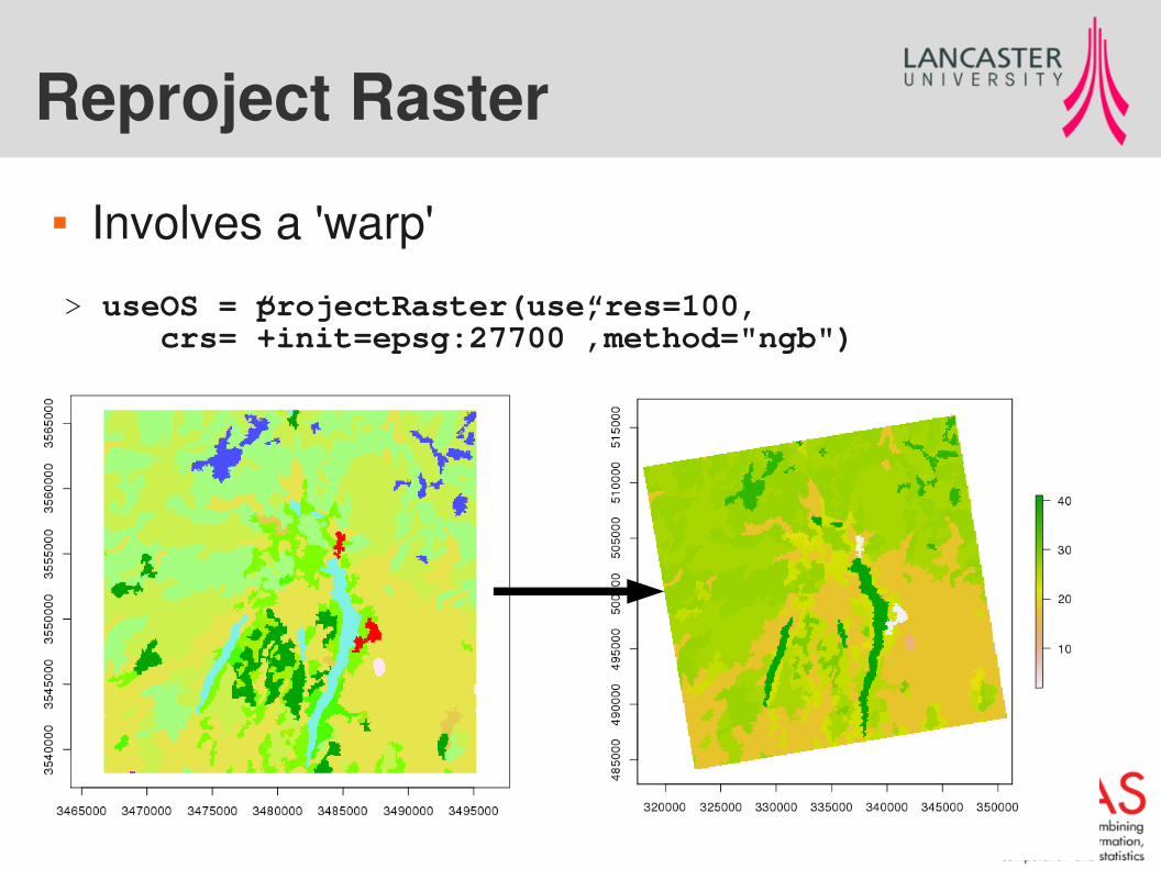
Reproject Raster
Involves a 'warp'
> useOS = projectRaster(use,res=100, crs=”+init=epsg:27700”,method="ngb")
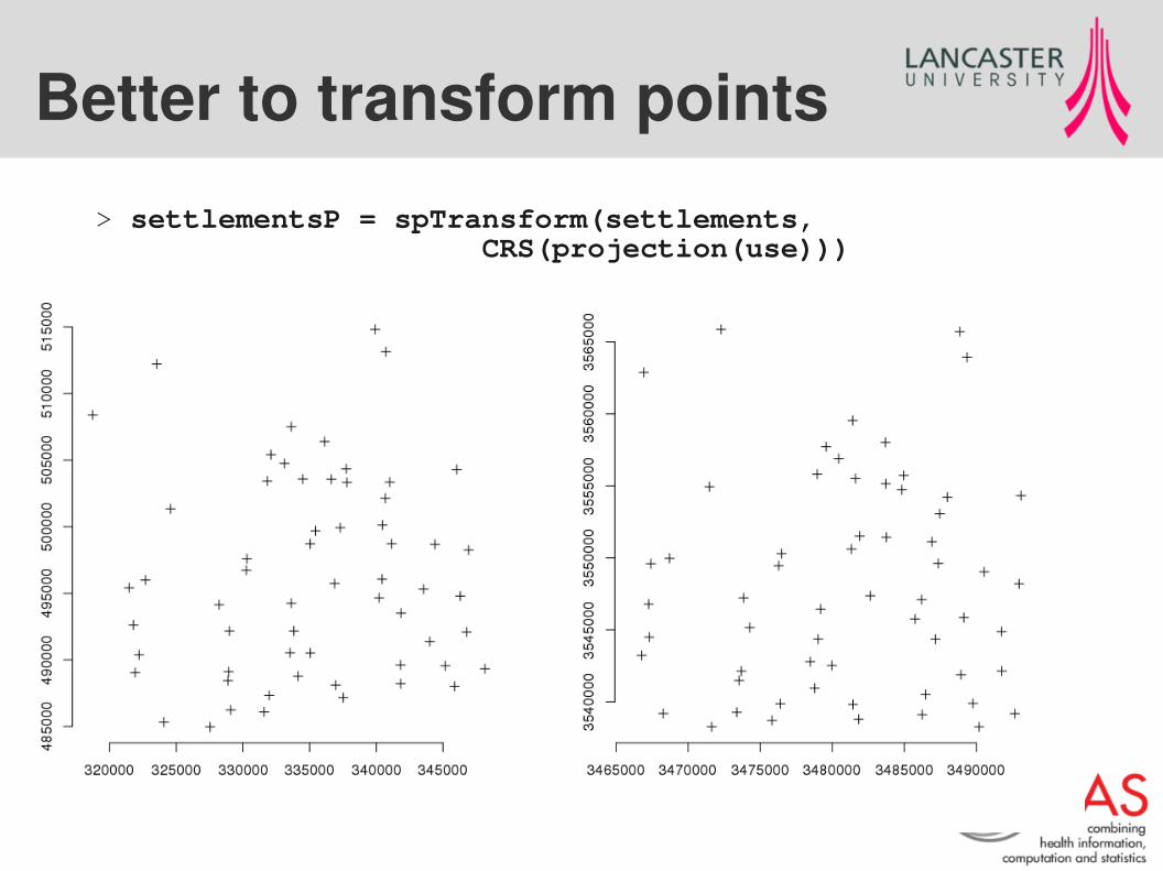
Better to transform points
> settlementsP = spTransform(settlements, CRS(projection(use)))
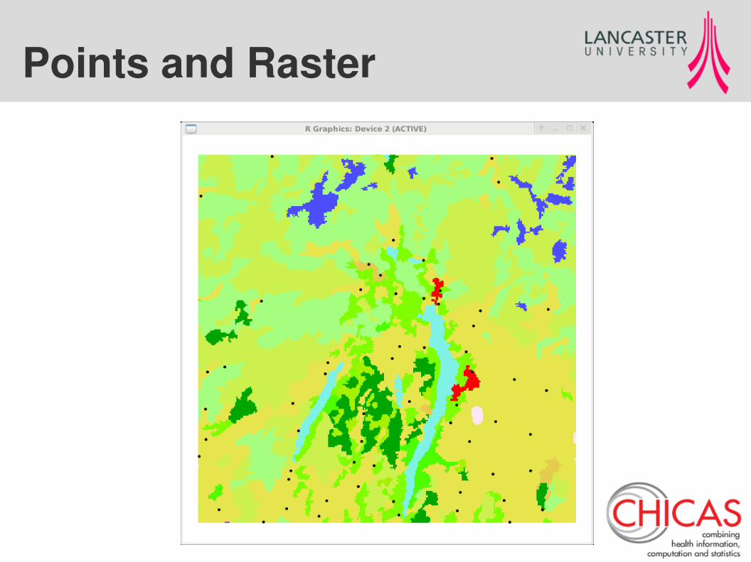
Points and Raster

Now lets go to work
Data created Coordinates corrected
Lets do some analysis!
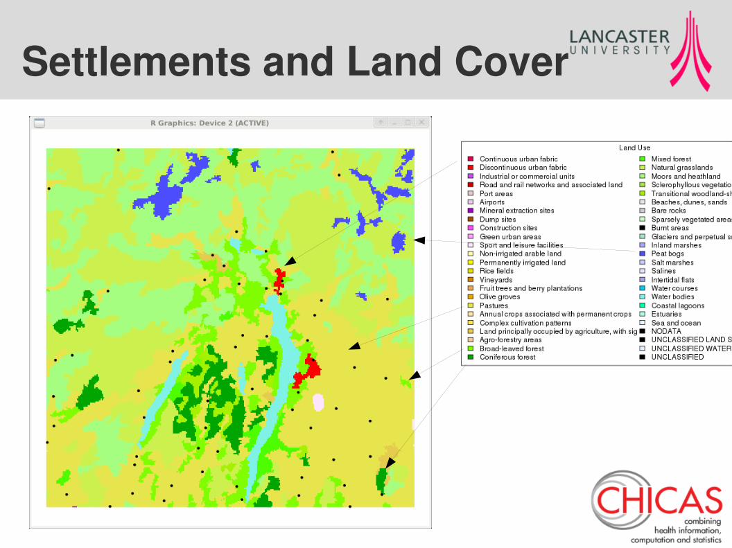
Settlements and Land Cover
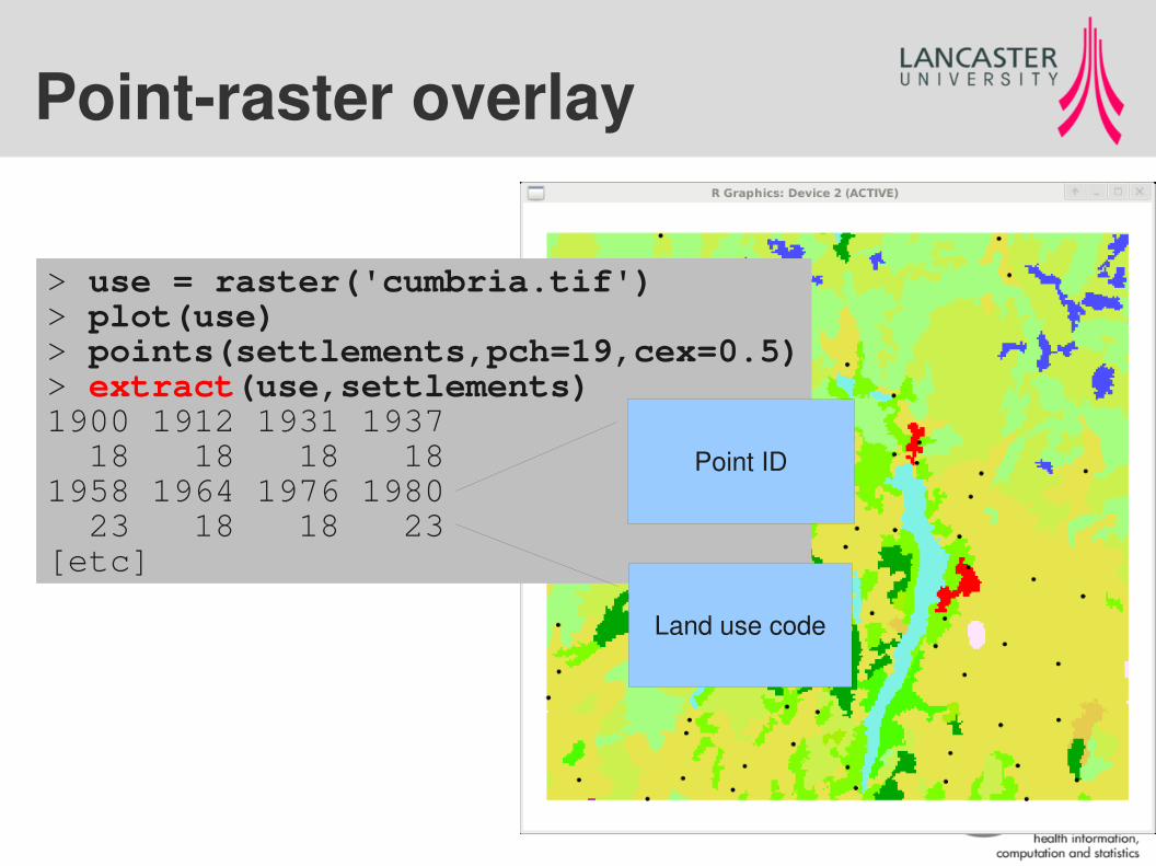
Point-raster overlay
> use = raster('cumbria.tif')> plot(use)> points(settlements,pch=19,cex=0.5)> extract(use,settlements)1900 1912 1931 1937 18 18 18 18 1958 1964 1976 1980 23 18 18 23[etc]
Point ID
Land use code
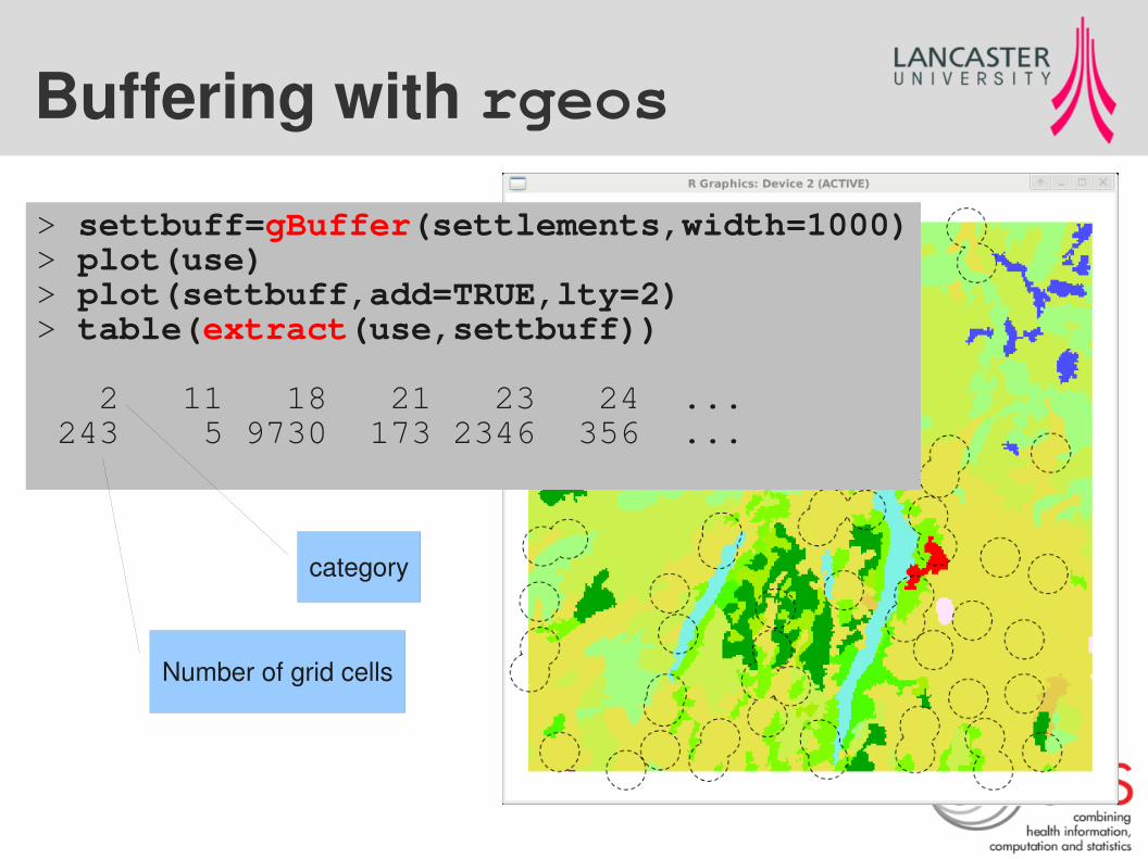
Buffering with rgeos
> settbuff=gBuffer(settlements,width=1000)> plot(use)> plot(settbuff,add=TRUE,lty=2)> table(extract(use,settbuff))
2 11 18 21 23 24 ... 243 5 9730 173 2346 356 ...
category
Number of grid cells
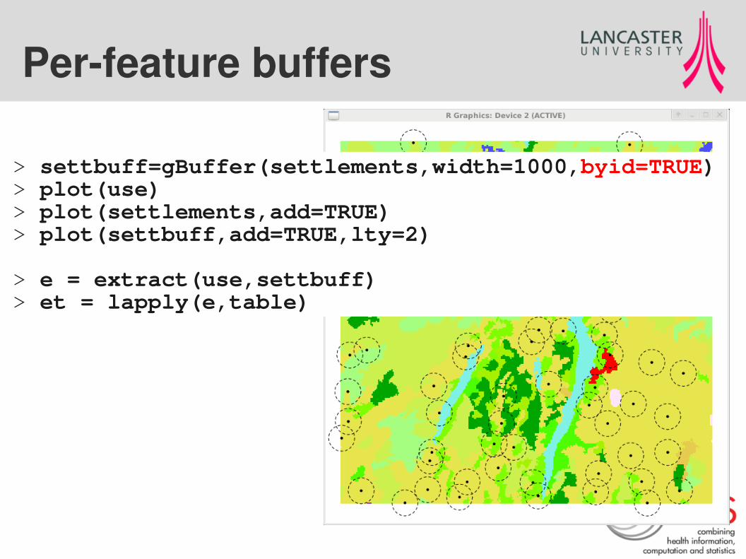
Per-feature buffers
> settbuff=gBuffer(settlements,width=1000,byid=TRUE)> plot(use)> plot(settlements,add=TRUE)> plot(settbuff,add=TRUE,lty=2)
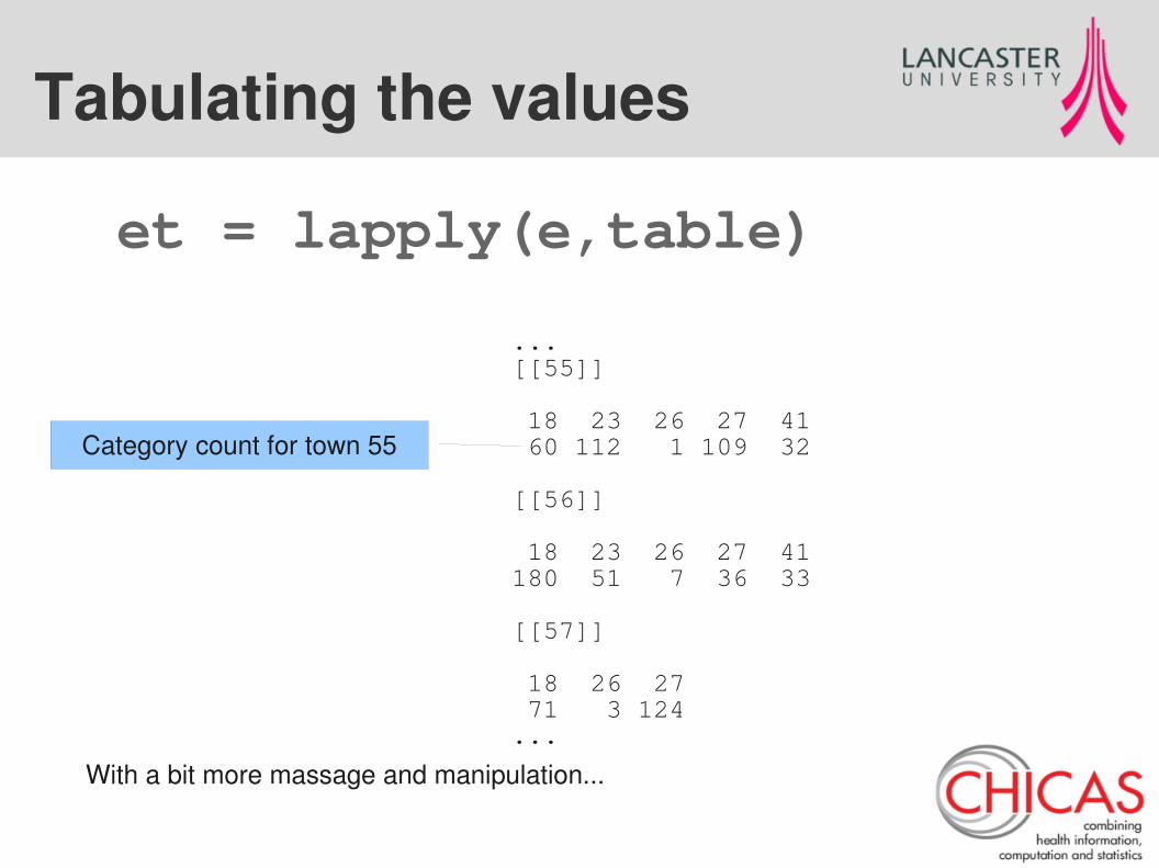
> e = extract(use,settbuff)> et = lapply(e,table)
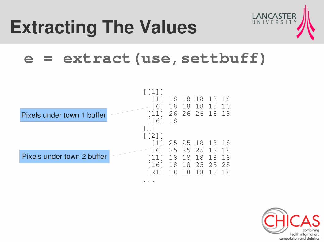
[[1]] [1] 18 18 18 18 18 [6] 18 18 18 18 18 [11] 26 26 26 18 18 [16] 18 […][[2]] [1] 25 25 18 18 18 [6] 25 25 25 18 18 [11] 18 18 18 18 18 [16] 18 18 25 25 25 [21] 18 18 18 18 18...
e = extract(use,settbuff)
Pixels under town 1 buffer
Pixels under town 2 buffer
Extracting The Values
Tabulating the values
...[[55]]
18 23 26 27 41 60 112 1 109 32
[[56]]
18 23 26 27 41 180 51 7 36 33
[[57]]
18 26 27 71 3 124 ...
et = lapply(e,table)
Category count for town 55
With a bit more massage and manipulation...
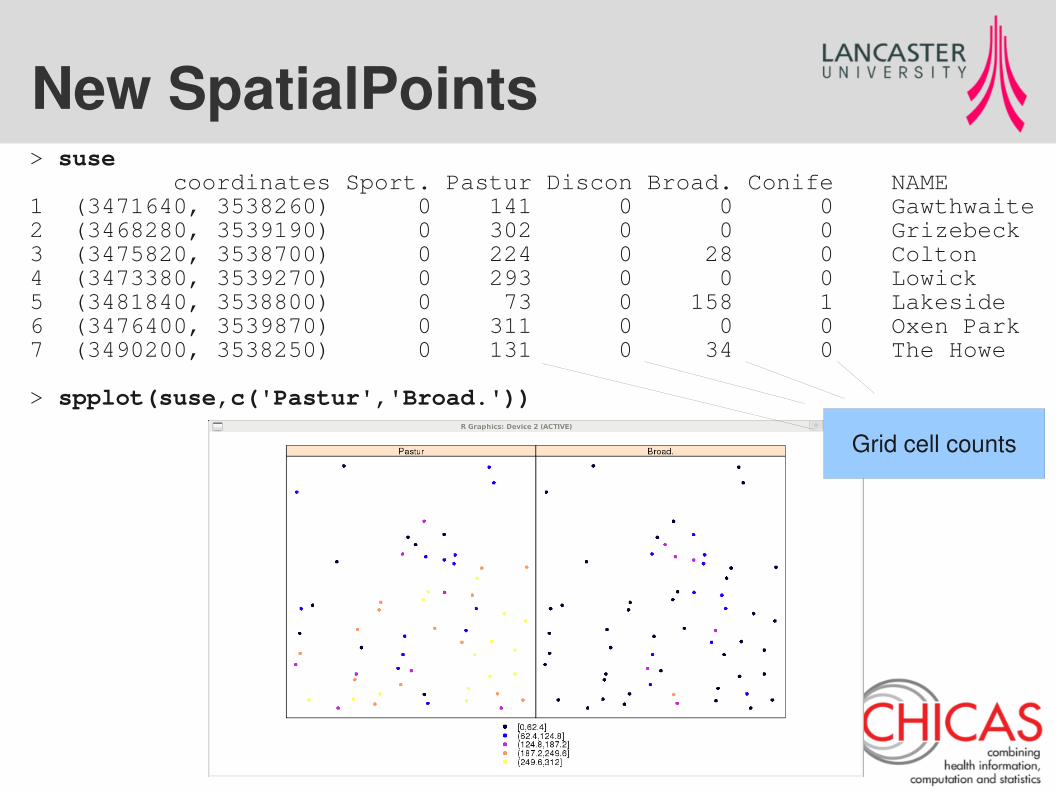
New SpatialPoints> suse coordinates Sport. Pastur Discon Broad. Conife NAME1 (3471640, 3538260) 0 141 0 0 0 Gawthwaite2 (3468280, 3539190) 0 302 0 0 0 Grizebeck3 (3475820, 3538700) 0 224 0 28 0 Colton4 (3473380, 3539270) 0 293 0 0 0 Lowick5 (3481840, 3538800) 0 73 0 158 1 Lakeside6 (3476400, 3539870) 0 311 0 0 0 Oxen Park7 (3490200, 3538250) 0 131 0 34 0 The Howe
> spplot(suse,c('Pastur','Broad.'))
Grid cell counts
Question
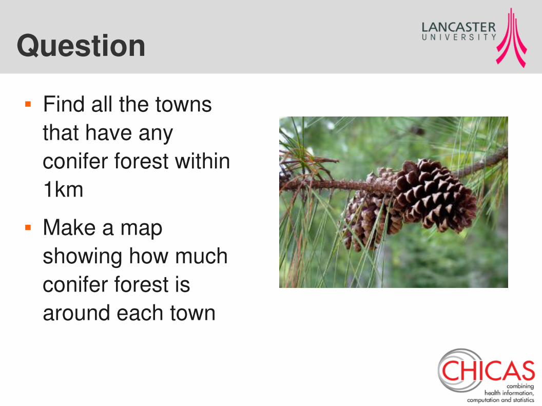
Find all the towns that have any conifer forest within 1km
Make a map showing how much conifer forest is around each town
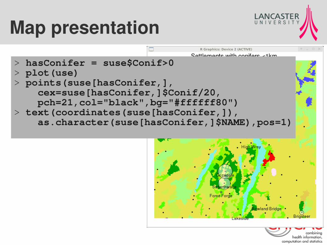
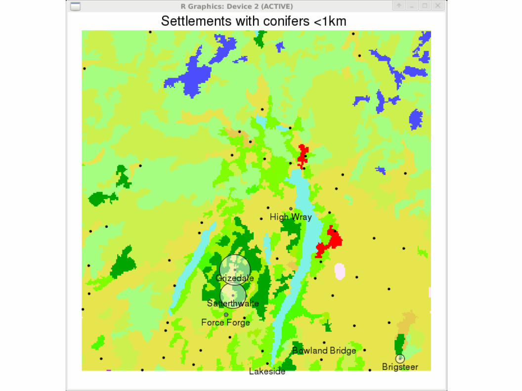
Map presentation
> hasConifer = suse$Conif>0> plot(use)> points(suse[hasConifer,], cex=suse[hasConifer,]$Conif/20, pch=21,col="black",bg="#ffffff80")> text(coordinates(suse[hasConifer,]), as.character(suse[hasConifer,]$NAME),pos=1)
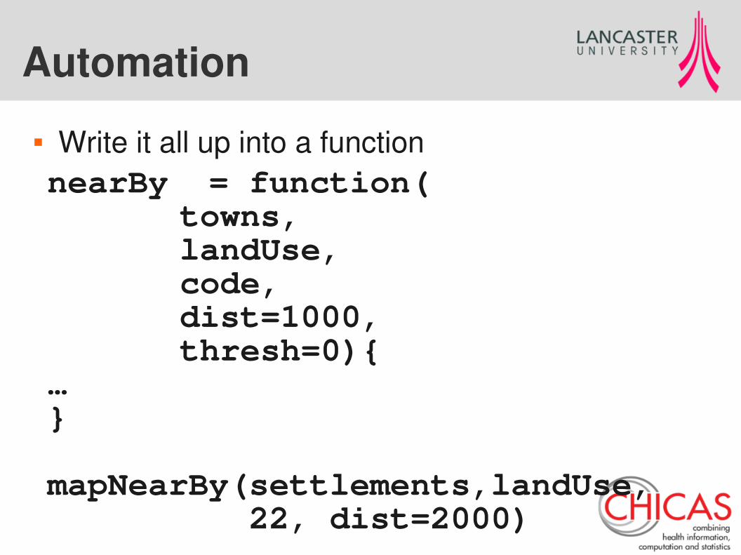
Automation
Write it all up into a functionnearBy = function(
towns,landUse,code,dist=1000,thresh=0){
…}
mapNearBy(settlements,landUse, 22, dist=2000)
Talk Title

End of Part One
Stay tuned for more!