GEOS-CHEM adjoint development using TAF

Monika Kopacz, Daniel Jacob, Dylan Jones (UT), Parvadha Suntharalingam, Paul Palmer

April 5, 2005

What is an adjoint model?

T

T T T

y K x

y K x K y x

( ) ( )

Y

TX

< y,Kx >

< K y, x >

Inverse map

For linear operator K, mapping from space X to space Y.

Adjoint operator KT

x y

K

K*

adjoint model

For nonlinear model K represents linearization of the original model

X Y

Why the need for adjoint model?O(101) O(105)

constraints on emissions with high resolution

can consider nonlinear processes

computationally efficient for sensitivity studies

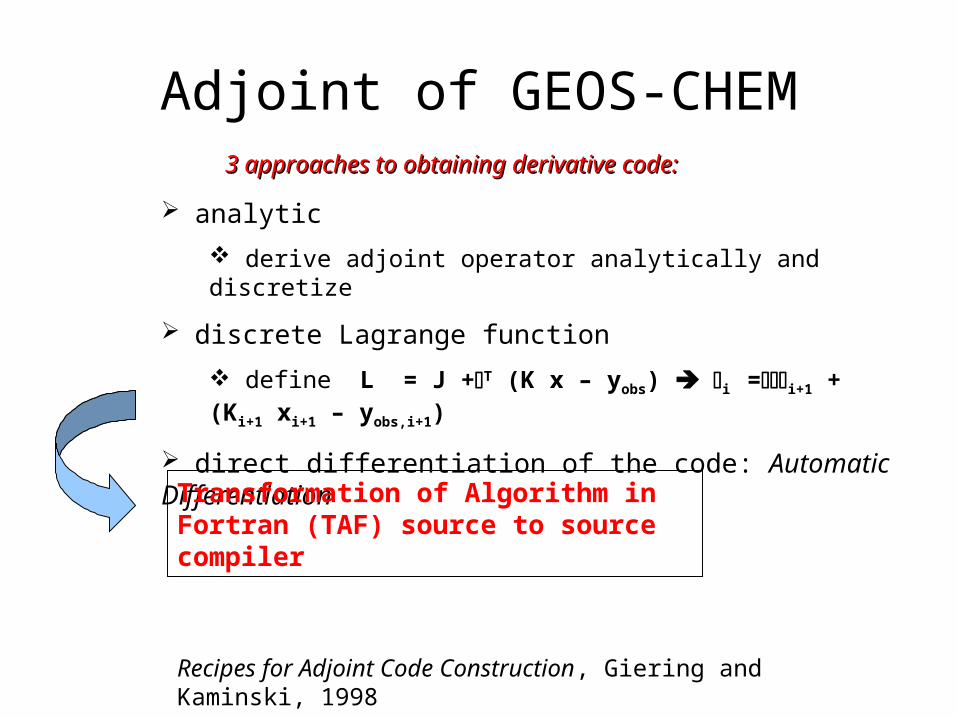
Adjoint of GEOS-CHEM3 approaches to obtaining derivative code:3 approaches to obtaining derivative code:

analytic

derive adjoint operator analytically and discretize

discrete Lagrange function

define L = J +T (K x – yobs) i =i+1 + (Ki+1 xi+1 – yobs,i+1)

direct differentiation of the code: Automatic Differentiation

Transformation of Algorithm in Fortran (TAF) source to source compiler

Recipes for Adjoint Code Construction, Giering and Kaminski, 1998

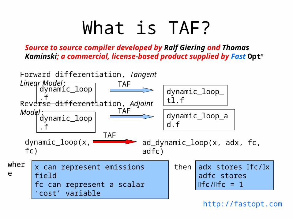
What is TAF?Source to source compiler developed by Ralf Giering and Thomas Kaminski; a commercial, license-based product supplied by Fast Opt®

Forward differentiation, Tangent Linear Model:

dynamic_loop.f dynamic_loop_tl.f

Reverse differentiation, Adjoint Model:

dynamic_loop.f dynamic_loop_ad.f

dynamic_loop(x, fc)TAF

ad_dynamic_loop(x, adx, fc, adfc)

adx stores fc/x adfc stores fc/fc = 1

where

http://fastopt.com

x can represent emissions fieldfc can represent a scalar ‘cost’ variable

then

TAF

TAF

Tangent Linear Model

verification: comparison with green’s function approach

Check linearity of the code

Resolve TAF-GC compatibility

Semi-automatically derived, stand-alone model

First step

challenges benefits

? general TAF-GC interfacing

? resolving flow nonlinearities

? Fortran 90 support

? manual changes

Adjoint Model

verification: comparison with previous CO inversions, (Heald et al. 2003, Palmer et al. 2003)

efficient sensitivity studies

J inversions for large state vector and large data sets

J data assimilation

Semi-automatically derived, stand-alone model

Next step

challenges benefits

? all TLM Fortran issues

? storage/recomputation for reverse mode

? non-trivial model evaluation

? manual changes

? Interfacing with optimization package

Minimizing the gradient

a priorifluxes

AdjointFluxes= J

AdjointTransport

GEOS-CHEM

GEOS-CHEM

MeasurementSampling

MeasurementSampling

EstimatedFluxes

ModeledConcentrations

simulatedConcentrations

ModeledMeasurements

“True”Measurements

AssumedMeasurement

Errors

WeightedMeasurement

Residuals

Cost functionJ

FluxUpdate

1 1( ) ( ) ( ) [ ( )] [ ( )]T Ta a aJ L L

x x x S x x y x S y x

0

°

°°

°

2

1

3

x2

x1

x3

x0

Minimum of cost function J

Courtesy of David Baker

Preliminary resultsFinite Difference Tangent Linear Model

y

x

3D field

Scalar perturbation

End product

ADJOINT MODELTANGENT LINEAR

MODEL

OPTIMIZATION PACKAGE

SEMI-AUTOMATIC CAPABILITY TO

GENERATE TLM/ADM

Automatic differentiation

1 1 1 1 1 1[ ( **2)]* [ * ( **2)*2* ]*l l l l l l lZ SIN Y X X COS Y Y Y

11 1 1 10 * ( **2)*2* ( **2)

0 1 0

0 0 1

l ll l l lZ X COS Y Y SIN Y Z

Y Y

X X

Z = X * SIN (Y**2)

differential

1

1 1 1

1

* 0 0 0 *

* * ( **2)*2* 1 0 *

* ( **2) 0 1 *

l l

l l l

l

Z Z

Y X COS Y Y Y

X SIN Y X

transpose

ADY = ADY + ADZ*X *COS(Y**2)*2*YADX = ADX + ADZ*SIN(Y**2)ADZ = 0.0

from Recipes for Adjoint Code Construction by R. Giering and T. Kaminski, 1998

Analytic adjoint operator for advection

dc du c u

dt dt L

TY X< y,Kx > < K y, x >

d

dtLConsider

[ ]y xx y

dc dcc c dt

dt dt [ ( ) ( ) ]x y x yc L c L c c dt

yxx y y x y x

dcdcc c c dt c c c dt

dt dt

[ ( ) ( ) ]x y x yc L c L c c dt

*d

dtL

**

dcu c

dt