1

Geos 223 Introductory Paleontology Spring 2006

Lab 2: Microfossils

Name:

Section:

AIMS:

This lab will introduce you to the main groups of microfossils found in Phanerozoic

rocks. There is also an exercise demonstrating how microfossils are used in

biostratigraphy. By the end of this lab you will able to distinguish each major microfossil

group, and have an appreciation for the significance and practical applications of

microfossils in paleontology.

PART A: GROUPS OF MICROFOSSILS.

Microfossils are fossils so small as to require a microscope for identification. Broadly

speaking, this includes all fossils less than 2 mm in size. This size fraction includes (1)

fully grown tiny organisms, (2) juvenile stages of larger organisms, (3) small anatomical

parts of larger organisms, and (4) incomplete fragments of larger organisms. This lab will

focus on microfossils of types (1) and (3), as these types are widely used for practical

applications such as biostratigraphy and paleoclimate/paleoenvironmental

reconstructions.

Common and important microscopic organisms falling into class (1) include

foraminifera, radiolaria, diatoms, coccolithophores, acritarchs, and ostracods. Conodonts

(the “teeth” of an extinct chordate group) provide an important example of type (3)

microfossils. These groups of organisms are of tremendous importance in modern and

ancient ecosystems, and their remains are prized in fields such as geology, paleobiology,

paleoclimatology, the evolutionary sciences, and even industry and construction. Make

sure that you can identify each group (drawing representative specimens might help), and

that you are familiar with their diversity, life modes, stratigraphic ranges, and practical

applications.

2

FORAMINIFERA:

Foraminifera (also called forams or foraminifers) are amoeba- like unicellular protists

(eukaryotes). They are typically 0.1 to 1.0 mm in size, but some could attain a relatively

enormous size of 100 mm. All forams are aquatic: most are marine, but they also occur in

fresh, brackish, and even hypersaline waters. Foram species can be either planktonic

(floating in water) or benthic (living on the sediment surface). Unambiguous foram

fossils are known from the Ordovician (questionable ones are known from the

Cambrian), and the group is still very abundant today.

Forams are preserved in the fossil record on account of their shell- like tests,

which have a high preservation potential. Different groups of forams have different types

of tests, so test composition and morphology (number and arrangement of chambers)

forms the basis for foram systematics. Forams are useful for high-resolution

biostratigraphy, for interpretation of paleoenvironments (e.g., temperature, water depth,

oxygen levels, etc.), and in microevolutionary studies. Forams have also achieved fame in

a rather accidental way: the famous Egyptian pyramids are made of large blocks of

Eocene (Tertiary) “nummulitic limestone” containing abundant foram fossils. (Indeed,

the fossil forams are called Nummulites gizehensis, named for the Gizah plateau where

they (and the pyramids) are found.)

A1. Mud from near the top of a sediment core from the modern Mediterranean Sea.

At the start of lab, Melanie will demonstrate how forams are extracted from such

unlithified core samples (washing and then sieving). By the end of lab the forams should

be ready for picking. This is painstaking work, and is done with a very fine paintbrush

while looking through a binocular stereomicroscope. The procedure for extracting

microfossils from rocks is similar, but often involves acids or other chemicals to

disaggregate or dissolve the matrix.

Approximately how many forams were in this 2cm3 sample?

3

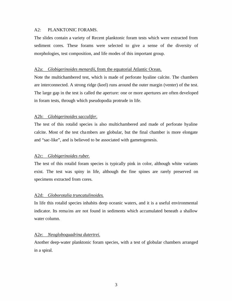
A2: PLANKTONIC FORAMS.

The slides contain a variety of Recent planktonic foram tests which were extracted from

sediment cores. These forams were selected to give a sense of the diversity of

morphologies, test composition, and life modes of this important group.

A2a: Globigerinoides menardii, from the equatorial Atlantic Ocean.

Note the multichambered test, which is made of perforate hyaline calcite. The chambers

are interconnected. A strong ridge (keel) runs around the outer margin (venter) of the test.

The large gap in the test is called the aperture: one or more apertures are often developed

in foram tests, through which pseudopodia protrude in life.

A2b: Globigerinoides sacculifer.

The test of this rotalid species is also multichambered and made of perforate hyaline

calcite. Most of the test chambers are globular, but the final chamber is more elongate

and “sac-like”, and is believed to be associated with gametogenesis.

A2c: Globigerinoides ruber.

The test of this rotalid foram species is typically pink in color, although white variants

exist. The test was spiny in life, although the fine spines are rarely preserved on

specimens extracted from cores.

A2d: Globorotalia truncatulinoides.

In life this rotalid species inhabits deep oceanic waters, and it is a useful environmental

indicator. Its remains are not found in sediments which accumulated beneath a shallow

water column.

A2e: Neogloboquadrina dutertrei.

Another deep-water planktonic foram species, with a test of globular chambers arranged

in a spiral.

4

A2f: Orbulina universa.

This foram secretes a tiny coiled test as a juvenile. At maturity, the spherical test seen

here is produced, and the juvenile test is either resorbed or entirely enclosed within the

mature orb. Note that there are no apertures in the mature test, which is again made of

perforate hyaline calcite.

A2g: Pulleniatina sp.

The test of this miliolid foram is porcelaneous rather than hyaline, and appears opaque

rather than glassy. It is also non-perforate. Forams with porcelaneous tests are known

from the Carboniferous to the Recent, while hyaline tests range back to the Silurian.

A3: BENTHIC FORAMS.

Benthic forms inhabited the seafloor in life. They tend to be larger than planktonic

species, and lack a strong keel. Their tests are typically not spiny.

A3a: Uvigerina sp.

The chambers of this test loosely resemble a bunch of grapes, and are ornamented with

strong ridges.

A3b: Cibididoides wuellerstorfi.

The multichambered test is coiled into a spiral resembling a miniature goniatite (see Lab

5).

A3c: Cibicides sp.

A benthic species with a shiny calcitic test.

A3d: Hoeglundina elegans.

The shiny test of this foram is made of aragonite rather than calcite.

5

Why would such a test not be found in Paleozoic rocks?

A3e: A textularid foram test.

What kind of test is represented here?

List two reasons why such tests are not constructed by planktonic forams.

A4: Triticites, a fusulinid foram (Pennsylvanian, Graham Formation, Texas).

Fusulinids are an important group of fossil forams, which ranged in time from the

Ordovician to the Permian. Fusulinids are the only foram group to have possessed a

microgranular calcareous test, which is characteristically shaped like a fat cigar or grain

of rice. Some fusulinids (like these) could attain large sizes. Fusulinids are used as zone

fossils in biostratigraphy to subdivide the Carboniferous and Permian periods.

Specimen A4b is a “fusulinid limestone”. This is a limestone rock containing abundant

and large fusulinid forams, visible with the naked eye. In some cases the internal

chambers of the test can be seen.

6

RADIOLARIA:

Like forams, radiolaria are small (typically 0.1 to 2 mm long) amoeba- like unicellular

protists (eukaryotes). They differ from forams most obviously by possessing siliceous

skeletons (rather than agglutinated or calcareous tests). All radiolaria are planktonic

heterotrophs, floating in the water column and using pseudopodia to move and feed.

Many contain photosynthesizing endosymbionts, permanently living within the

radiolarian cell cytoplasm. These endosymbionts provide food and oxygen (through

photosynthesis) to the host radiolarian, but obviously require light to do so. Host

radiolaria are therefore confined to sunlit waters (the “photic zone”, less than 200 meters

below sea level in perfectly clear water). Radiolarian fossils are known from the

Cambrian, and the group is still very common today.

The siliceous radiolarian skeleton (the fossilizable portion of the organism) is

often highly complex and beautiful to look at. It can often consist of very delicate spines

and rays; some skeletons are ball- like, and such spheres can be nested one within another.

Some skeletons are conical and look almost “helmet- like”. The skeleton has many pores,

which reduces the weight of the structure and is beneficial for a planktonic mode of life.

A5. Radiolaria of various ages.

These slides show a variety of beautiful fossil and Recent radiolaria skeletons. Note the

diverse shapes of the perforate skeletons.

A5a. Recent radiolaria.

A5b. Tertiary radiolaria.

A5c. Cretaceous radiolaria.

A5d. Jurassic radiolaria.

The geologically older specimens appear “frosted” or of a different color to the Recent

and Tertiary examples. Why might this be?

7

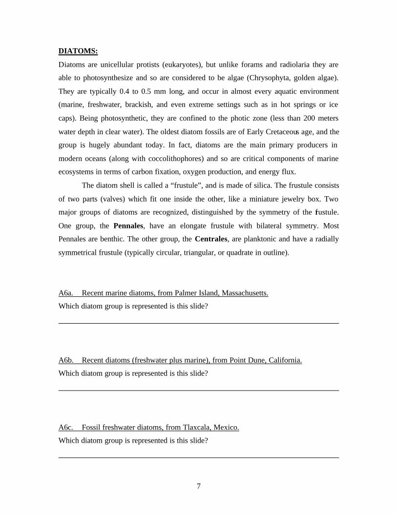
DIATOMS:

Diatoms are unicellular protists (eukaryotes), but unlike forams and radiolaria they are

able to photosynthesize and so are considered to be algae (Chrysophyta, golden algae).

They are typically 0.4 to 0.5 mm long, and occur in almost every aquatic environment

(marine, freshwater, brackish, and even extreme settings such as in hot springs or ice

caps). Being photosynthetic, they are confined to the photic zone (less than 200 meters

water depth in clear water). The oldest diatom fossils are of Early Cretaceous age, and the

group is hugely abundant today. In fact, diatoms are the main primary producers in

modern oceans (along with coccolithophores) and so are critical components of marine

ecosystems in terms of carbon fixation, oxygen production, and energy flux.

The diatom shell is called a “frustule”, and is made of silica. The frustule consists

of two parts (valves) which fit one inside the other, like a miniature jewelry box. Two

major groups of diatoms are recognized, distinguished by the symmetry of the frustule.

One group, the Pennales, have an elongate frustule with bilateral symmetry. Most

Pennales are benthic. The other group, the Centrales, are planktonic and have a radially

symmetrical frustule (typically circular, triangular, or quadrate in outline).

A6a. Recent marine diatoms, from Palmer Island, Massachusetts.

Which diatom group is represented is this slide?

A6b. Recent diatoms (freshwater plus marine), from Point Dune, California.

Which diatom group is represented is this slide?

A6c. Fossil freshwater diatoms, from Tlaxcala, Mexico.

Which diatom group is represented is this slide?

8

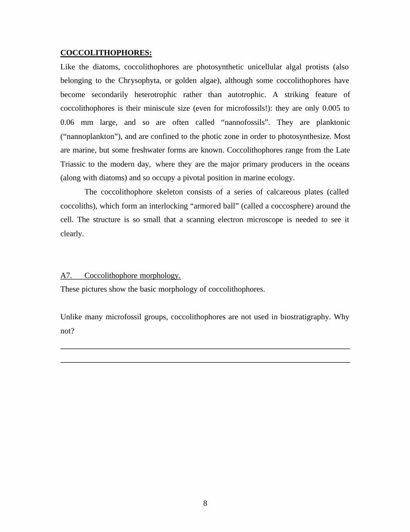
COCCOLITHOPHORES:

Like the diatoms, coccolithophores are photosynthetic unicellular algal protists (also

belonging to the Chrysophyta, or golden algae), although some coccolithophores have

become secondarily heterotrophic rather than autotrophic. A striking feature of

coccolithophores is their miniscule size (even for microfossils!): they are only 0.005 to

0.06 mm large, and so are often called “nannofossils”. They are planktonic

(“nannoplankton”), and are confined to the photic zone in order to photosynthesize. Most

are marine, but some freshwater forms are known. Coccolithophores range from the Late

Triassic to the modern day, where they are the major primary producers in the oceans

(along with diatoms) and so occupy a pivotal position in marine ecology.

The coccolithophore skeleton consists of a series of calcareous plates (called

coccoliths), which form an interlocking “armored ball” (called a coccosphere) around the

cell. The structure is so small that a scanning electron microscope is needed to see it

clearly.

A7. Coccolithophore morphology.

These pictures show the basic morphology of coccolithophores.

Unlike many microfossil groups, coccolithophores are not used in biostratigraphy. Why

not?

9

ACRITARCHS:

Acritarchs are also unicellular protistan algae, although their precise evolutionary

relationships are unknown (they may be green algae or dinoflagellate algae). They are

small (0.02 to 0.05 mm) organic spheres, common in rocks of Precambrian (at least 1900

million years old) to Recent age. All are planktonic. Acritarchs are sufficiently common

in late Precambrian rocks that they are used as biostratigraphic zone fossils.

A8. Acritarch morphology.

Note that the surface of the acritarchs can be smooth or spiny. The earliest fossil

acritarchs were all smooth, but spiny forms evolved and became dominant in the Late

Neoproterozoic. List two potential selective advantages of possessing spines.

What might have triggered the rise to prevalence of spiny acritarchs over smooth

acritarchs in the Late Neoproterozoic?

10

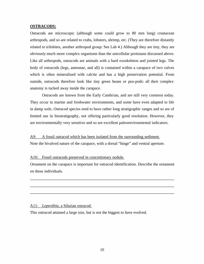
OSTRACODS:

Ostracods are microscopic (although some could grow to 80 mm long) crustacean

arthropods, and so are related to crabs, lobsters, shrimp, etc. (They are therefore distantly

related to trilobites, another arthropod group: See Lab 4.) Although they are tiny, they are

obviously much more complex organisms than the unicellular protistans discussed above.

Like all arthropods, ostracods are animals with a hard exoskeleton and jointed legs. The

body of ostracods (legs, antennae, and all) is contained within a carapace of two valves

which is often mineralized with calcite and has a high preservation potential. From

outside, ostracods therefore look like tiny green beans or pea-pods: all their complex

anatomy is tucked away inside the carapace.

Ostracods are known from the Early Cambrian, and are still very common today.

They occur in marine and freshwater environments, and some have even adapted to life

in damp soils. Ostracod species tend to have rather long stratigraphic ranges and so are of

limited use in biostratigraphy, not offering particularly good resolution. However, they

are environmentally very sensitive and so are excellent paleoenvironmental indicators.

A9: A fossil ostracod which has been isolated from the surrounding sediment.

Note the bivalved nature of the carapace, with a dorsal “hinge” and ventral aperture.

A10: Fossil ostracods preserved in concretionary nodule.

Ornament on the carapace is important for ostracod identification. Describe the ornament

on these individuals.

A11: Leperditia, a Silurian ostracod.

This ostracod attained a large size, but is not the biggest to have evolved.

11

CONODONTS:

Unlike all the microfossil groups discussed above, conodont microfossils do not represent

the fossilized remains of an entire microscopic organism. Instead, conodonts are

microscopic teeth-like elements of a larger organism (the conodont animal). Conodont

means “cone tooth”.

Conodont elements are tiny structures (typically 0.5 to 1.0 mm long) made of

calcium phosphate (apatite). Although they look and functioned like teeth, their internal

microstructure shows that the elements grew on all surfaces and so are different to teeth

such as ours. Three major morphologies can be recognized: cone- like elements

(coniform), bar- like elements (ramiform), and platform-like elements (pectiniform). The

conodont animal possessed a fierce- looking array of all three types, each type presumably

having a particular biting function (much like the arrangement of incisors, canines,

premolars, and molars in your mouth). Conodont fossils are known from the Cambrian to

the Triassic: the conodont animal apparently became extinct at that time.

Conodonts are extremely useful for biostratigraphy. Coniform elements evolved

rapidly in the Ordovician, and allow biostratigraphic zones to be established with average

durations of 4 million years. Similarly, platform elements in the Devonian and

Carboniferous allow biostratigraphic zones to be established with average durations of

only 1 million years. Conodonts also serve a practical use in oil exploration, as their color

darkens predictably as a function of diagenetic heating. Since oil grade is also determined

by the extent of diagenetic heating, conodonts are often examined for color when

decisions as to whether or not to drill for oil are made.

A12: Conodont morphology and literature.

12

PART B: MICROFOSSILS, BIOSTRATIGRAPHY, AND CORRELATION.

One of the most important practical applications of micropaleontology is the use of

microfossils in biostratigraphy. This is the concept whereby geological time can be

subdivided according to the ranges of species in the fossil record. A species evolves once,

survives for a time, and then becomes extinct. A rock containing that fossil species is

assumed to have been deposited during the interval of geologic time between the

origination and extinction of that species. By ranking the order of appearance of different

species through time, it is possible to subdivide geologic time biostratigraphically. Thus

if species B evolved before species C but after species A, rocks containing species A but

lacking species B must be older than rocks containing species B. Similarly, rocks

containing species B (with or without species A) but lacking species C must be older than

rocks containing species C.

Furthermore, because the same species will never re-evolve at a later time, all

rocks containing a given species can be assumed to have been deposited during the time

that species was extant (alive), no matter where those rocks are found. Finding the same

species in rocks at different localities tells us those rocks are of the same age: this is

called correlation.

Microfossils are excellent for biostratigraphy and correlation. This is because

microfossils are very abundant (being so small, there are many specimens per rock

sample), they had a high rate of evolution (many speciation events, so many potential

biostratigraphic zones), and they often had very wide geographic distributions (the same

species could be found in many areas, permitting correlation across a big area).

The following exercise is based upon real data from a study of Miocene (Tertiary)

diatoms from two localities in southern California. We will use this exercise to see how

biostratigraphy and correlation is done.

Background:

During the Miocene (23.5 to 5.14 million years ago), sea level was higher than it is today.

Areas presently quite far inland were below sea level, and were sites of deposition of

marine sedimentary rocks. These rocks are now exposed subaerially, and can be collected

for fossils. In the 1970s, a student called John Barron conducted his PhD thesis at UCLA,

13

trying to work out the biostratigraphy of Miocene sediments in southern California using

diatoms fossilized in those sediments. His research was later published (Barron, J. A.,

1975, Marine diatom biostratigraphy of the Upper Miocene-Lower Pliocene strata of

southern California, Journal of Paleontology 49: 619-632). Data from that paper are used

here.

Miocene rocks at two localities (Newport Beach and Lompoc; Figure B1) were

collected for microfossils. Each diatom was identified, and the precise level in the

measured section from which each fossil was recovered was noted (see Appendix 1). The

study involves addressing three questions:

1. What is the order of appearance of diatom species at Newport Beach during the

Miocene?

2. What is the order of appearance of diatom species at Lompoc over the same

interval?

3. How does the order of appearance of these species compare at each locality? Only

species occurring in the same order at each locality can be used to

biostratigraphically subdivide the Miocene rocks in this region. We will use a

method known as “graphic correlation” to investigate this.

14

Figure B1: Map of study area in southern California, showing location of Newport Beach and Lompoc sections.

First, we must work out the order of appearance of each diatom species at each

locality. The fossil identifications and stratigraphic occurrences are listed in Appendix 1.

Note that each species of diatom (16 in total) has been given a letter code for ease of

reading. The key to each species code is given in Appendix 2.

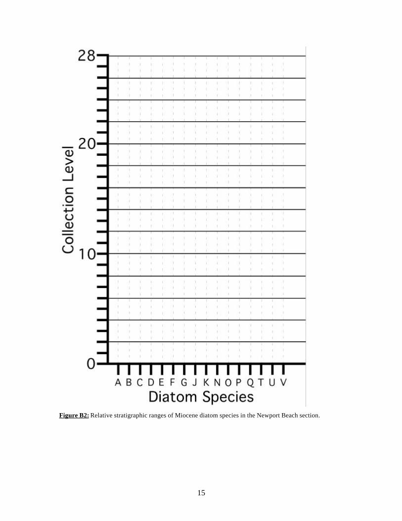
B1. On Figure B2, draw a biostratigraphic range chart for each diatom species at the

Newport Beach Section (data in Appendix 1). Note that Figure 2 plots the fossil horizons

as ranked ordinal levels (i.e., drawn as if equally spaced), not in terms of their actual

meterage on the rock outcrop. For each species, draw a vertical line connecting its lowest

occurrence to its highest occurrence: this represents the known stratigraphic range of that

species.

15

Figure B2: Relative stratigraphic ranges of Miocene diatom species in the Newport Beach section.

16

B2. You can see that species do not always occur at all fossil horizons between their first

and last occurrence at Newport Beach. Given that species do not go extinct and then re-

evolve, why could these “gaps” in species ranges occur?

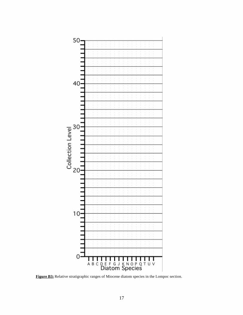
B3. On Figure B3, draw a biostratigraphic range chart for each diatom species at the

Lompoc Section (data in Appendix 1). For each species, draw a vertical line connecting

its lowest occurrence to its highest occurrence: this represents the known stratigraphic

range of that species.

Biostratigraphic zonation of geologic time is achieved by correlating the first appearance

of a species across localities. Biostratigraphic zones are never defined in terms of the last

occurrence (i.e., time of extinction) of a species. In order to correlate these two Miocene

sections, we must therefore first work out the order of appearance of the various species

at each section (i.e., work out which species appeared before which others).

B4. In the left-hand empty column of Table B1, list the lowest collection horizon at

which each of the 16 diatom species was found in the Newport Beach section (e.g., if the

lowest occurrence of a species was in horizon 3, enter a “3” in the cell).

B5. In the right-hand empty column of Table B1, list the lowest collection horizon at

which each of the 16 diatom species was found in the Lompoc section.

17

Figure B3: Relative stratigraphic ranges of Miocene diatom species in the Lompoc section.

18

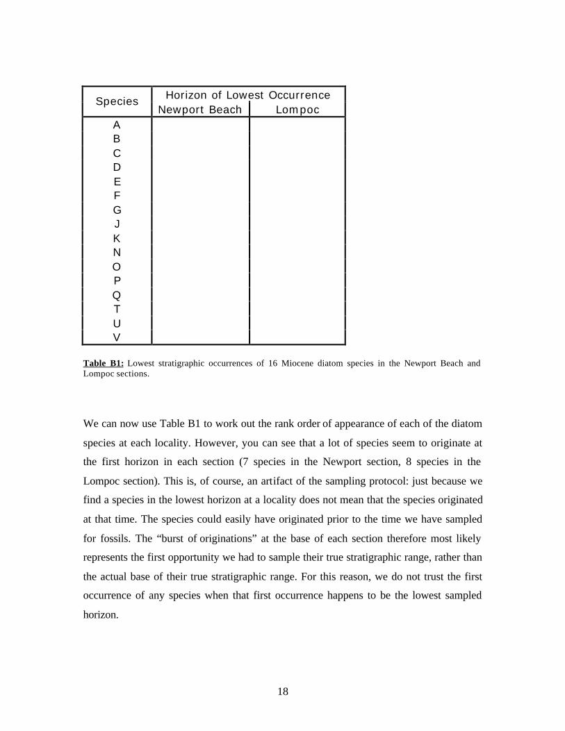
Horizon of Lowest Occurrence Species Newport Beach Lompoc

A B C D E F G J K N O P Q T U V

Table B1: Lowest stratigraphic occurrences of 16 Miocene diatom species in the Newport Beach and Lompoc sections.

We can now use Table B1 to work out the rank order of appearance of each of the diatom

species at each locality. However, you can see that a lot of species seem to originate at

the first horizon in each section (7 species in the Newport section, 8 species in the

Lompoc section). This is, of course, an artifact of the sampling protocol: just because we

find a species in the lowest horizon at a locality does not mean that the species originated

at that time. The species could easily have originated prior to the time we have sampled

for fossils. The “burst of originations” at the base of each section therefore most likely

represents the first opportunity we had to sample their true stratigraphic range, rather than

the actual base of their true stratigraphic range. For this reason, we do not trust the first

occurrence of any species when that first occurrence happens to be the lowest sampled

horizon.

19

B6. In Table B1, lightly shade in both cells next to any species which made its lowest

appearance at horizon 1 in either of the sections. These are the species for which we have

no reliable estimate of the true first appearance at one or both localities, and these must

be ignored in our correlation.

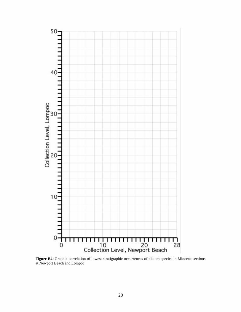
B7. Now we can correlate the sections! On Figure B4, plot the horizon of first occurrence

at Newport Beach against the horizon of first occurrence at Lompoc for each species,

using the data from the unshaded cells in Table B1. For example, species F first occurs at

horizon 6 in the Newport Beach section and at horizon 4 in the Lompoc section: place a

point representing species F at coordinate (6, 4) on the graph. Label that point with a

small letter “F”. Repeat this procedure for all species with unshaded cells in Table B1,

labeling each point with its species code.

B8. Join the points you have plotted on Figure B4. Join points which lie at successively

higher values along the x-axis (Newport Beach section).

The graph you have just drawn is a GRAPHIC CORRELATION of the two localities.

The line connecting the points traces the sequence of first occurrences of species in the

Newport Beach section. You will see that the line does not slope evenly across the graph:

the slope changes, and even zigzags up and down in successive points on the y-axis

(Lompoc section).

B9: What does this zigzag mean, in terms of the order of first appearances of species at

each locality?

20

Figure B4: Graphic correlation of lowest stratigraphic occurrences of diatom species in Miocene sections at Newport Beach and Lompoc.

21

B10. How do you explain this zigzag?

B11. Use the graphic correlation plotted in Figure B4 to define biostratigraphic zones for

the Miocene of southern California. Remember that a biostratigraphic zone must be

defined in terms of the first occurrence of a particular species, and that the order of zones

must be the same in all localities. How many zones can you identify? Which species

define each zone?

22

Appendix 1:

Stratigraphic occurrences of diatom species in the Miocene sections at Newport Beach

and Lompoc, southern California. Fossil horizons at each locality are numbered in rank

order of stratigraphic level (1 being oldest). The Newport Beach section is 289 meters

thick and contained 28 fossiliferous horizons. The Lompoc section is 511 meters thick

and contained 50 fossiliferous horizons. Diatom species occurring at each fossil horizon

are coded as letters: the key to the codes is given in Appendix 2.

Newport Beach Section:

1 1 m above base of section: B, D, E, O, P, U, V. 2 3 m above base of section: A, B, D, E, O, P, U, V. 3 12 m above base of section: A, B, C, D, E, O, P, V. 4 13 m above base of section: D, E, O, P. 5 17 m above base of section: D, E, K, P, V. 6 35 m above base of section: D, E, F, K, P, V. 7 41 m above base of section: D, F, K, O, P. 8 67 m above base of section: F, G, K, O, P, U. 9 69 m above base of section: J, O, P, U, V. 10 85 m above base of section: G, J. 11 88 m above base of section: J, U. 12 109 m above base of section: G, J, N. 13 123 m above base of section: G, J, N. 14 132 m above base of section: G, J, K, N, U. 15 142 m above base of section: G, J, K, N, V. 16 153 m above base of section: G, J, K, N. 17 162 m above base of section: J, N, U. 18 177 m above base of section: J. 19 191 m above base of section: J, N, Q, U. 20 203 m above base of section: J. 21 213 m above base of section: J, Q. 22 221 m above base of section: J. 23 222 m above base of section: J, U. 24 237 m above base of section: J, Q, T, U, V. 25 248 m above base of section: J, Q, V. 26 253 m above base of section: J, Q. 27 260 m above base of section: J, Q. 28 289 m above base of section: J.

23

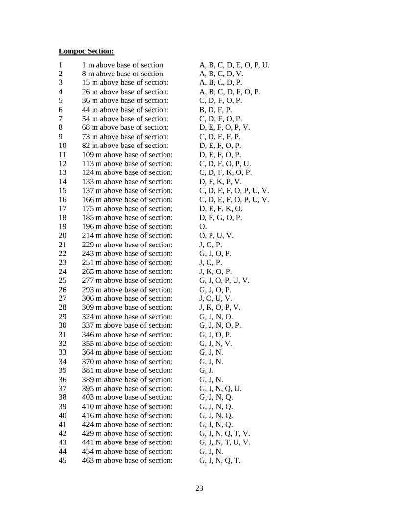
Lompoc Section:

1 1 m above base of section: A, B, C, D, E, O, P, U. 2 8 m above base of section: A, B, C, D, V. 3 15 m above base of section: A, B, C, D, P. 4 26 m above base of section: A, B, C, D, F, O, P. 5 36 m above base of section: C, D, F, O, P. 6 44 m above base of section: B, D, F, P. 7 54 m above base of section: C, D, F, O, P. 8 68 m above base of section: D, E, F, O, P, V. 9 73 m above base of section: C, D, E, F, P. 10 82 m above base of section: D, E, F, O, P. 11 109 m above base of section: D, E, F, O, P. 12 113 m above base of section: C, D, F, O, P, U. 13 124 m above base of section: C, D, F, K, O, P. 14 133 m above base of section: D, F, K, P, V. 15 137 m above base of section: C, D, E, F, O, P, U, V. 16 166 m above base of section: C, D, E, F, O, P, U, V. 17 175 m above base of section: D, E, F, K, O. 18 185 m above base of section: D, F, G, O, P. 19 196 m above base of section: O. 20 214 m above base of section: O, P, U, V. 21 229 m above base of section: J, O, P. 22 243 m above base of section: G, J, O, P. 23 251 m above base of section: J, O, P. 24 265 m above base of section: J, K, O, P. 25 277 m above base of section: G, J, O, P, U, V. 26 293 m above base of section: G, J, O, P. 27 306 m above base of section: J, O, U, V. 28 309 m above base of section: J, K, O, P, V. 29 324 m above base of section: G, J, N, O. 30 337 m above base of section: G, J, N, O, P. 31 346 m above base of section: G, J, O, P. 32 355 m above base of section: G, J, N, V. 33 364 m above base of section: G, J, N. 34 370 m above base of section: G, J, N. 35 381 m above base of section: G, J. 36 389 m above base of section: G, J, N. 37 395 m above base of section: G, J, N, Q, U. 38 403 m above base of section: G, J, N, Q. 39 410 m above base of section: G, J, N, Q. 40 416 m above base of section: G, J, N, Q. 41 424 m above base of section: G, J, N, Q. 42 429 m above base of section: G, J, N, Q, T, V. 43 441 m above base of section: G, J, N, T, U, V. 44 454 m above base of section: G, J, N. 45 463 m above base of section: G, J, N, Q, T.

24

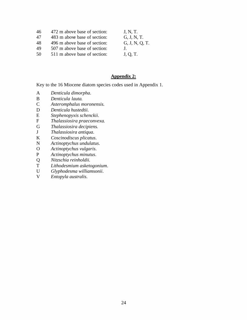
46 472 m above base of section: J, N, T. 47 483 m above base of section: G, J, N, T. 48 496 m above base of section: G, J, N, Q, T. 49 507 m above base of section: J. 50 511 m above base of section: J, Q, T.

Appendix 2:

Key to the 16 Miocene diatom species codes used in Appendix 1.

A Denticula dimorpha. B Denticula lauta. C Asteromphalus moronensis. D Denticula hustedtii. E Stephenopyxis schenckii. F Thalassiosira praeconvexa. G Thalassiosira decipiens. J Thalassiosira antiqua. K Coscinodiscus plicatus. N Actinoptychus undulatus. O Actinoptychus vulgaris. P Actinoptychus minutus. Q Nitzschia reinholdii. T Lithodesmium asketogonium. U Glyphodesma williamsonii. V Entopyla australis.