Embed Size (px)
Citation preview
.
.
.
.
.
.
.
.
.
.
.
.
.
.
.
.
.
.
.
.
.
.
.
.
.
.
.
.
.
.
.
.
.
.
.
.
.
.
.
.
Part I: Decision making under uncertainty
Georg Ch. PflugEES-UETP
July 3, 2016
Georg Ch. PflugEES-UETP Part I: Decision making under uncertainty
.
.
.
.
.
.
.
.
.
.
.
.
.
.
.
.
.
.
.
.
.
.
.
.
.
.
.
.
.
.
.
.
.
.
.
.
.
.
.
.
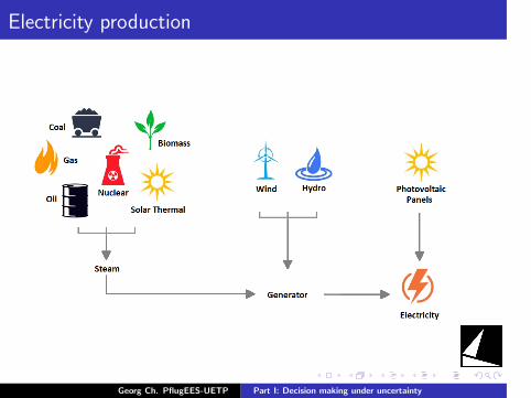
Electricity production
Georg Ch. PflugEES-UETP Part I: Decision making under uncertainty
.
.
.
.
.
.
.
.
.
.
.
.
.
.
.
.
.
.
.
.
.
.
.
.
.
.
.
.
.
.
.
.
.
.
.
.
.
.
.
.
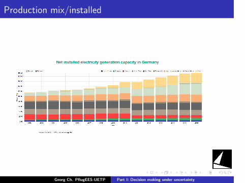
Production mix/installed
Georg Ch. PflugEES-UETP Part I: Decision making under uncertainty
.
.
.
.
.
.
.
.
.
.
.
.
.
.
.
.
.
.
.
.
.
.
.
.
.
.
.
.
.
.
.
.
.
.
.
.
.
.
.
.
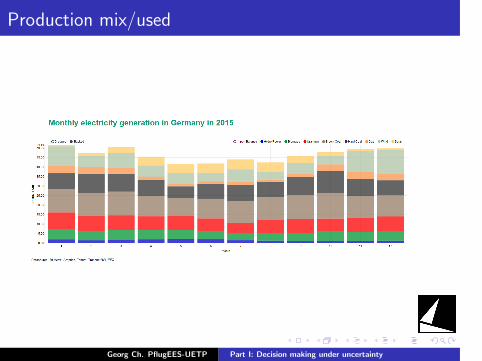
Production mix/used
Georg Ch. PflugEES-UETP Part I: Decision making under uncertainty
.
.
.
.
.
.
.
.
.
.
.
.
.
.
.
.
.
.
.
.
.
.
.
.
.
.
.
.
.
.
.
.
.
.
.
.
.
.
.
.
Georg Ch. PflugEES-UETP Part I: Decision making under uncertainty
.
.
.
.
.
.
.
.
.
.
.
.
.
.
.
.
.
.
.
.
.
.
.
.
.
.
.
.
.
.
.
.
.
.
.
.
.
.
.
.
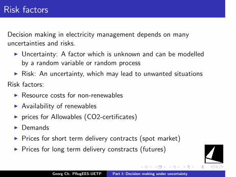
Risk factors
Decision making in electricity management depends on manyuncertainties and risks.
I Uncertainty: A factor which is unknown and can be modelledby a random variable or random process
I Risk: An uncertainty, which may lead to unwanted situations
Risk factors:
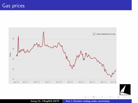
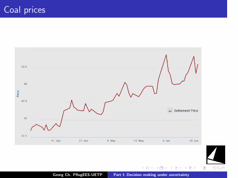
I Resource costs for non-renewables
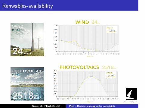
I Availability of renewables
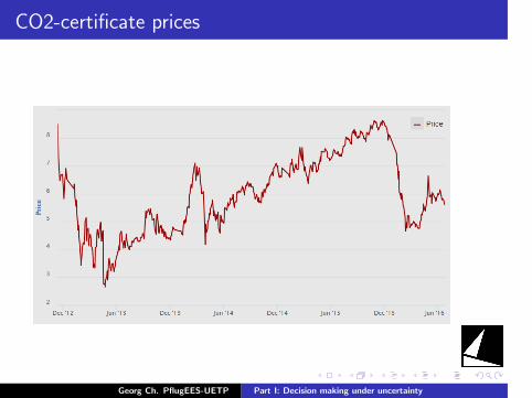
I prices for Allowables (CO2-certificates)
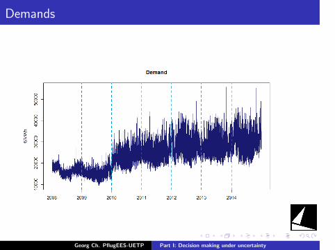
I Demands
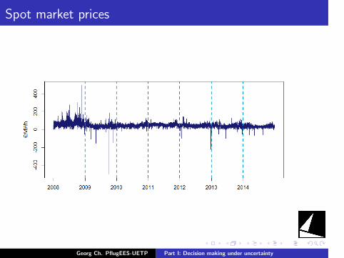
I Prices for short term delivery contracts (spot market)
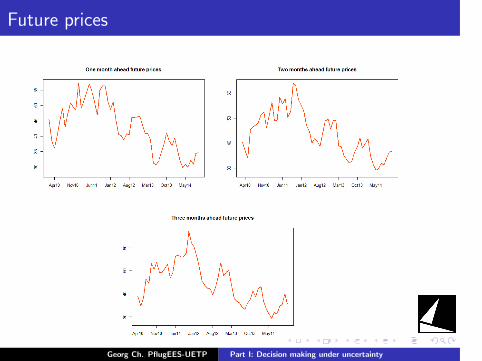
I Prices for long term delivery constracts (futures)
Georg Ch. PflugEES-UETP Part I: Decision making under uncertainty
.
.
.
.
.
.
.
.
.
.
.
.
.
.
.
.
.
.
.
.
.
.
.
.
.
.
.
.
.
.
.
.
.
.
.
.
.
.
.
.
Gas prices
Georg Ch. PflugEES-UETP Part I: Decision making under uncertainty
.
.
.
.
.
.
.
.
.
.
.
.
.
.
.
.
.
.
.
.
.
.
.
.
.
.
.
.
.
.
.
.
.
.
.
.
.
.
.
.
Coal prices
Georg Ch. PflugEES-UETP Part I: Decision making under uncertainty
.
.
.
.
.
.
.
.
.
.
.
.
.
.
.
.
.
.
.
.
.
.
.
.
.
.
.
.
.
.
.
.
.
.
.
.
.
.
.
.
Renwables-availability
Georg Ch. PflugEES-UETP Part I: Decision making under uncertainty
.
.
.
.
.
.
.
.
.
.
.
.
.
.
.
.
.
.
.
.
.
.
.
.
.
.
.
.
.
.
.
.
.
.
.
.
.
.
.
.
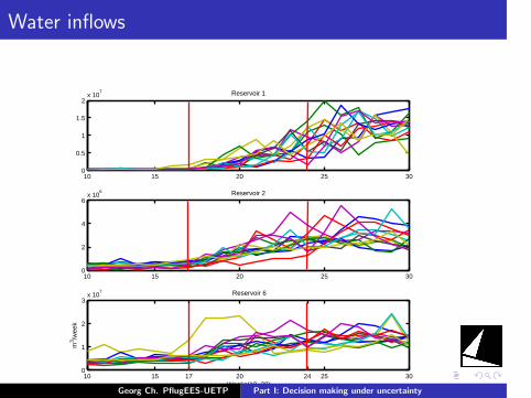
Water inflows
10 15 20 25 300
0.5
1
1.5
2x 10
7 Reservoir 1
10 15 20 25 300
2
4
6x 10
6 Reservoir 2
10 15 17 20 24 25 300
1
2
3x 10
7
Weeks(10−30)
m3 /w
eek
Reservoir 6
Georg Ch. PflugEES-UETP Part I: Decision making under uncertainty
.
.
.
.
.
.
.
.
.
.
.
.
.
.
.
.
.
.
.
.
.
.
.
.
.
.
.
.
.
.
.
.
.
.
.
.
.
.
.
.
CO2-certificate prices
Georg Ch. PflugEES-UETP Part I: Decision making under uncertainty
.
.
.
.
.
.
.
.
.
.
.
.
.
.
.
.
.
.
.
.
.
.
.
.
.
.
.
.
.
.
.
.
.
.
.
.
.
.
.
.
Demands
Georg Ch. PflugEES-UETP Part I: Decision making under uncertainty
.
.
.
.
.
.
.
.
.
.
.
.
.
.
.
.
.
.
.
.
.
.
.
.
.
.
.
.
.
.
.
.
.
.
.
.
.
.
.
.
Spot market prices
Georg Ch. PflugEES-UETP Part I: Decision making under uncertainty
.
.
.
.
.
.
.
.
.
.
.
.
.
.
.
.
.
.
.
.
.
.
.
.
.
.
.
.
.
.
.
.
.
.
.
.
.
.
.
.
Future prices
Georg Ch. PflugEES-UETP Part I: Decision making under uncertainty
.
.
.
.
.
.
.
.
.
.
.
.
.
.
.
.
.
.
.
.
.
.
.
.
.
.
.
.
.
.
.
.
.
.
.
.
.
.
.
.
Stochastic optimization
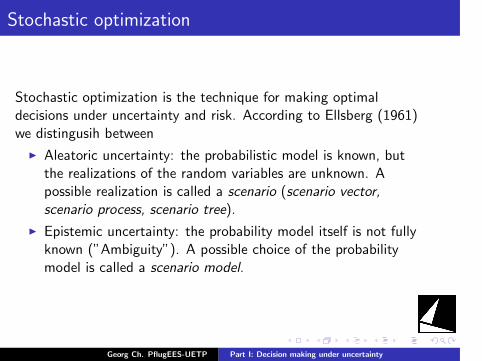
Stochastic optimization is the technique for making optimaldecisions under uncertainty and risk. According to Ellsberg (1961)we distingusih between
I Aleatoric uncertainty: the probabilistic model is known, butthe realizations of the random variables are unknown. Apossible realization is called a scenario (scenario vector,scenario process, scenario tree).
I Epistemic uncertainty: the probability model itself is not fullyknown (”Ambiguity”). A possible choice of the probabilitymodel is called a scenario model.
Georg Ch. PflugEES-UETP Part I: Decision making under uncertainty
.
.
.
.
.
.
.
.
.
.
.
.
.
.
.
.
.
.
.
.
.
.
.
.
.
.
.
.
.
.
.
.
.
.
.
.
.
.
.
.
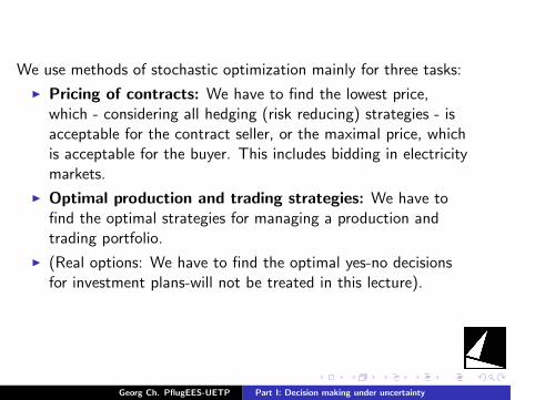
We use methods of stochastic optimization mainly for three tasks:
I Pricing of contracts: We have to find the lowest price,which - considering all hedging (risk reducing) strategies - isacceptable for the contract seller, or the maximal price, whichis acceptable for the buyer. This includes bidding in electricitymarkets.
I Optimal production and trading strategies: We have tofind the optimal strategies for managing a production andtrading portfolio.
I (Real options: We have to find the optimal yes-no decisionsfor investment plans-will not be treated in this lecture).
Georg Ch. PflugEES-UETP Part I: Decision making under uncertainty
.
.
.
.
.
.
.
.
.
.
.
.
.
.
.
.
.
.
.
.
.
.
.
.
.
.
.
.
.
.
.
.
.
.
.
.
.
.
.
.
The lecture plan
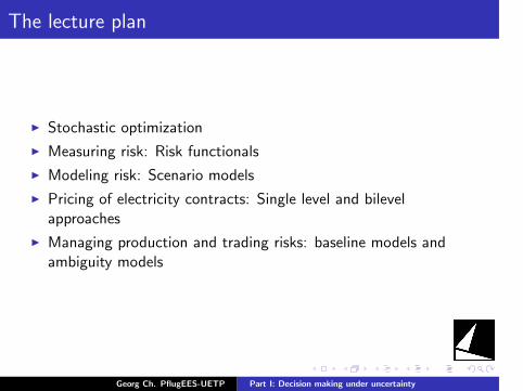
I Stochastic optimization
I Measuring risk: Risk functionals
I Modeling risk: Scenario models
I Pricing of electricity contracts: Single level and bilevelapproaches
I Managing production and trading risks: baseline models andambiguity models
Georg Ch. PflugEES-UETP Part I: Decision making under uncertainty
.
.
.
.
.
.
.
.
.
.
.
.
.
.
.
.
.
.
.
.
.
.
.
.
.
.
.
.
.
.
.
.
.
.
.
.
.
.
.
.
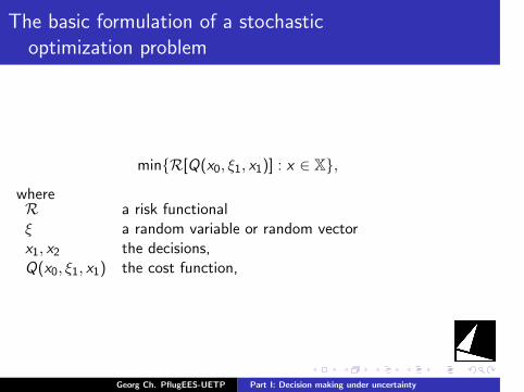
The basic formulation of a stochasticoptimization problem
minR[Q(x0, ξ1, x1)] : x ∈ X,
whereR a risk functionalξ a random variable or random vectorx1, x2 the decisions,Q(x0, ξ1, x1) the cost function,
Georg Ch. PflugEES-UETP Part I: Decision making under uncertainty
.
.
.
.
.
.
.
.
.
.
.
.
.
.
.
.
.
.
.
.
.
.
.
.
.
.
.
.
.
.
.
.
.
.
.
.
.
.
.
.
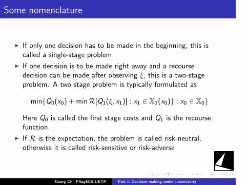
Some nomenclature
I If only one decision has to be made in the beginning, this iscalled a single-stage problem
I If one decision is to be made right away and a recoursedecision can be made after observing ξ, this is a two-stageproblem. A two stage problem is typically formulated as
minQ0(x0) + minR[Q1(ξ, x1)] : x1 ∈ X1(x0) : x0 ∈ X0
Here Q0 is called the first stage costs and Q1 is the recoursefunction.
I If R is the expectation, the problem is called risk-neutral,otherwise it is called risk-sensitive or risk-adverse
Georg Ch. PflugEES-UETP Part I: Decision making under uncertainty
.
.
.
.
.
.
.
.
.
.
.
.
.
.
.
.
.
.
.
.
.
.
.
.
.
.
.
.
.
.
.
.
.
.
.
.
.
.
.
.
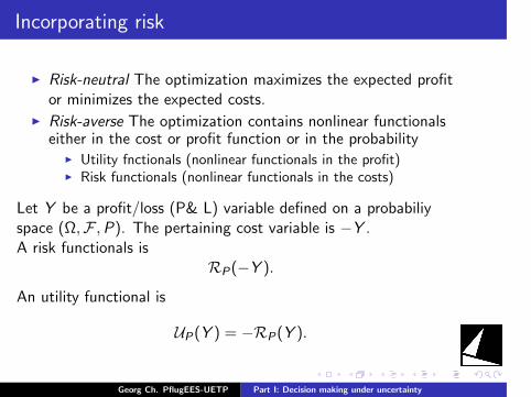
Incorporating risk
I Risk-neutral The optimization maximizes the expected profitor minimizes the expected costs.
I Risk-averse The optimization contains nonlinear functionalseither in the cost or profit function or in the probability
I Utility fnctionals (nonlinear functionals in the profit)I Risk functionals (nonlinear functionals in the costs)
Let Y be a profit/loss (P& L) variable defined on a probabiliyspace (Ω,F ,P). The pertaining cost variable is −Y .A risk functionals is
RP(−Y ).
An utility functional is
UP(Y ) = −RP(Y ).
Georg Ch. PflugEES-UETP Part I: Decision making under uncertainty
.
.
.
.
.
.
.
.
.
.
.
.
.
.
.
.
.
.
.
.
.
.
.
.
.
.
.
.
.
.
.
.
.
.
.
.
.
.
.
.
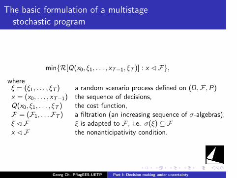
The basic formulation of a multistagestochastic program
minR[Q(x0, ξ1, . . . , xT−1, ξT )] : x F,
whereξ = (ξ1, . . . , ξT ) a random scenario process defined on (Ω,F ,P)x = (x0, . . . , xT−1) the sequence of decisions,Q(x0, ξ1, . . . , ξT ) the cost function,F = (F1, . . .FT ) a filtration (an increasing sequence of σ-algebras),ξ F ξ is adapted to F , i.e. σ(ξ) ⊆ Fx F the nonanticipativity condition.
Georg Ch. PflugEES-UETP Part I: Decision making under uncertainty
.
.
.
.
.
.
.
.
.
.
.
.
.
.
.
.
.
.
.
.
.
.
.
.
.
.
.
.
.
.
.
.
.
.
.
.
.
.
.
.
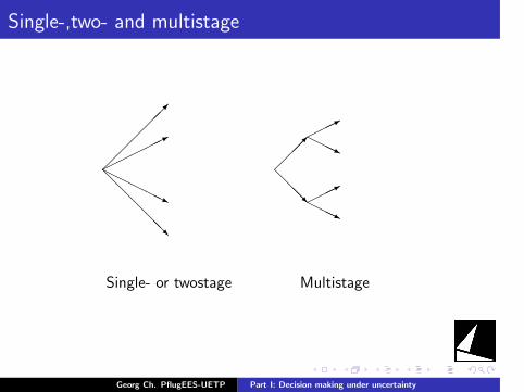
Single-,two- and multistage
*
@@@@@R
HHHHHj
@@@R
*HHHj
*HHHj
Single- or twostage Multistage
Georg Ch. PflugEES-UETP Part I: Decision making under uncertainty
.
.
.
.
.
.
.
.
.
.
.
.
.
.
.
.
.
.
.
.
.
.
.
.
.
.
.
.
.
.
.
.
.
.
.
.
.
.
.
.
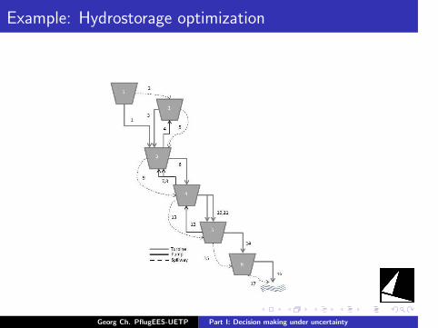
Example: Hydrostorage optimization
Georg Ch. PflugEES-UETP Part I: Decision making under uncertainty
.
.
.
.
.
.
.
.
.
.
.
.
.
.
.
.
.
.
.
.
.
.
.
.
.
.
.
.
.
.
.
.
.
.
.
.
.
.
.
.
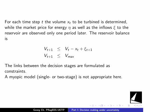
For each time step t the volume xt to be turbined is determined,while the market price for energy η as well as the inflows ξ to thereservoir are observed only one period later. The reservoir balanceis
Vt+1 ≤ Vt − xt + ξt+1
Vt+1 ≤ Vmax
The links between the decision stages are formulated asconstraints.A myopic model (single- or two-stage) is not appropriate here.
Georg Ch. PflugEES-UETP Part I: Decision making under uncertainty
.
.
.
.
.
.
.
.
.
.
.
.
.
.
.
.
.
.
.
.
.
.
.
.
.
.
.
.
.
.
.
.
.
.
.
.
.
.
.
.
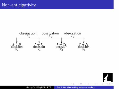
Non-anticipativity
? ? ? ?decision decision decision decision
x0 x1 x2 x3
t = 0 t = t1 t = t2 t = t3
observation observation observationF1 F2 F3
Georg Ch. PflugEES-UETP Part I: Decision making under uncertainty
.
.
.
.
.
.
.
.
.
.
.
.
.
.
.
.
.
.
.
.
.
.
.
.
.
.
.
.
.
.
.
.
.
.
.
.
.
.
.
.
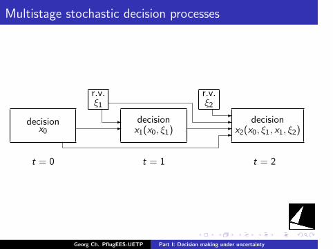
Multistage stochastic decision processes
decisionx0
r.v.ξ1
decisionx1(x0, ξ1)
r.v.ξ2
decisionx2(x0, ξ1, x1, ξ2)-
-- -
--
t = 0 t = 1 t = 2
Georg Ch. PflugEES-UETP Part I: Decision making under uncertainty

.
.
.
.
.
.
.
.
.
.
.
.
.
.
.
.
.
.
.
.
.
.
.
.
.
.
.
.
.
.
.
.
.
.
.
.
.
.
.
.
Linear stochastic recourse problems
min c0(x0) + Eξ1 [min c1(x1, ξ1)] : (x0, x1) ∈ X
where the feasible set X is given by
W0x0 ≥ h0
A1 x0 +W1 x1 ≥ h1(ξ1)
Georg Ch. PflugEES-UETP Part I: Decision making under uncertainty
.
.
.
.
.
.
.
.
.
.
.
.
.
.
.
.
.
.
.
.
.
.
.
.
.
.
.
.
.
.
.
.
.
.
.
.
.
.
.
.
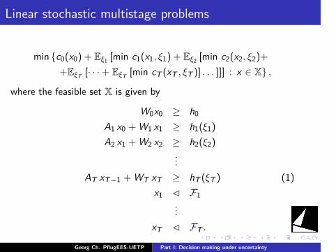
Linear stochastic multistage problems
min c0(x0) + Eξ1 [min c1(x1, ξ1) + Eξ2 [min c2(x2, ξ2)+
+EξT [· · ·+ EξT [min cT (xT , ξT )] . . . ]]] : x ∈ X ,
where the feasible set X is given by
W0x0 ≥ h0
A1 x0 +W1 x1 ≥ h1(ξ1)
A2 x1 +W2 x2 ≥ h2(ξ2)...
AT xT−1 +WT xT ≥ hT (ξT ) (1)
x1 F1
...
xT FT .
Georg Ch. PflugEES-UETP Part I: Decision making under uncertainty
.
.
.
.
.
.
.
.
.
.
.
.
.
.
.
.
.
.
.
.
.
.
.
.
.
.
.
.
.
.
.
.
.
.
.
.
.
.
.
.
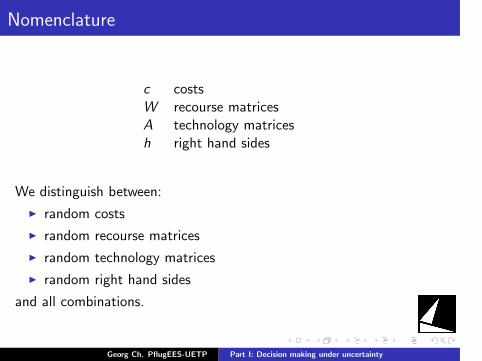
Nomenclature
c costsW recourse matricesA technology matricesh right hand sides
We distinguish between:
I random costs
I random recourse matrices
I random technology matrices
I random right hand sides
and all combinations.
Georg Ch. PflugEES-UETP Part I: Decision making under uncertainty
.
.
.
.
.
.
.
.
.
.
.
.
.
.
.
.
.
.
.
.
.
.
.
.
.
.
.
.
.
.
.
.
.
.
.
.
.
.
.
.
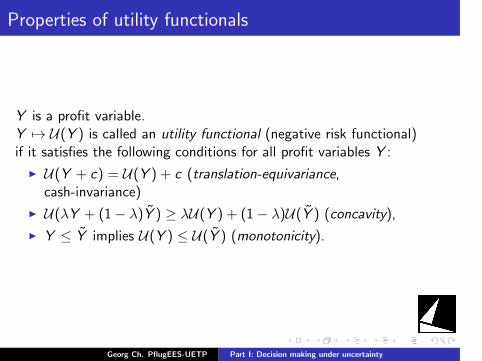
Properties of utility functionals
Y is a profit variable.Y 7→ U(Y ) is called an utility functional (negative risk functional)if it satisfies the following conditions for all profit variables Y :
I U(Y + c) = U(Y ) + c (translation-equivariance,cash-invariance)
I U(λY + (1− λ)Y ) ≥ λU(Y ) + (1− λ)U(Y ) (concavity),
I Y ≤ Y implies U(Y ) ≤ U(Y ) (monotonicity).
Georg Ch. PflugEES-UETP Part I: Decision making under uncertainty
.
.
.
.
.
.
.
.
.
.
.
.
.
.
.
.
.
.
.
.
.
.
.
.
.
.
.
.
.
.
.
.
.
.
.
.
.
.
.
.
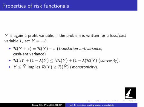
Properties of risk functionals
Y is again a profit variable, if the problem is written for a loss/costvariable L, set Y = −L.
I R(Y + c) = R(Y )− c (translation-antivariance,cash-antivariance)
I R(λY + (1− λ)Y ) ≤ λR(Y ) + (1− λ)R(Y ) (convexity),
I Y ≤ Y implies R(Y ) ≥ R(Y ) (monotonicity).
Georg Ch. PflugEES-UETP Part I: Decision making under uncertainty
.
.
.
.
.
.
.
.
.
.
.
.
.
.
.
.
.
.
.
.
.
.
.
.
.
.
.
.
.
.
.
.
.
.
.
.
.
.
.
.
More Definitions
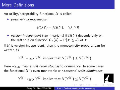
An utility/acceptability functional U is called
I positively homogeneous if
U(λY ) = λU(Y ), ∀λ ≥ 0
I version-independent (law-invariant) if U(Y ) depends only onthe distribution function GY (u) = PY ≤ u of Y .
If U is version independent, then the monotonicity property can bewritten as
Y (1) ≺FSD Y (2) implies that U(Y (1)) ≤ U(Y (2))
Here ≺FSD means first order stochastic dominance. In some casesthe functional U is even monotonic w.r.t.second order dominance
Y (1) ≺SSD Y (2) implies that U(Y (1)) ≤ U(Y (2))
Georg Ch. PflugEES-UETP Part I: Decision making under uncertainty
.
.
.
.
.
.
.
.
.
.
.
.
.
.
.
.
.
.
.
.
.
.
.
.
.
.
.
.
.
.
.
.
.
.
.
.
.
.
.
.
Order relations
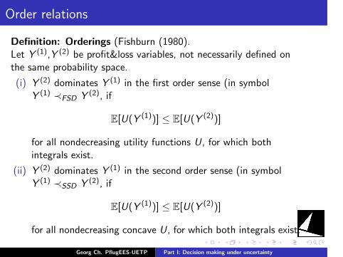
Definition: Orderings (Fishburn (1980).Let Y (1),Y (2) be profit&loss variables, not necessarily defined onthe same probability space.
(i) Y (2) dominates Y (1) in the first order sense (in symbolY (1) ≺FSD Y (2), if
E[U(Y (1))] ≤ E[U(Y (2))]
for all nondecreasing utility functions U, for which bothintegrals exist.
(ii) Y (2) dominates Y (1) in the second order sense (in symbolY (1) ≺SSD Y (2), if
E[U(Y (1))] ≤ E[U(Y (2))]
for all nondecreasing concave U, for which both integrals exist.
Georg Ch. PflugEES-UETP Part I: Decision making under uncertainty
.
.
.
.
.
.
.
.
.
.
.
.
.
.
.
.
.
.
.
.
.
.
.
.
.
.
.
.
.
.
.
.
.
.
.
.
.
.
.
.
0 1 2 3 40
0.1
0.2
0.3
0.4
0.5
0.6
0.7
0.8
0.9
1
0 1 2 3 40
0.5
1
1.5
2
2.5
3
3.5
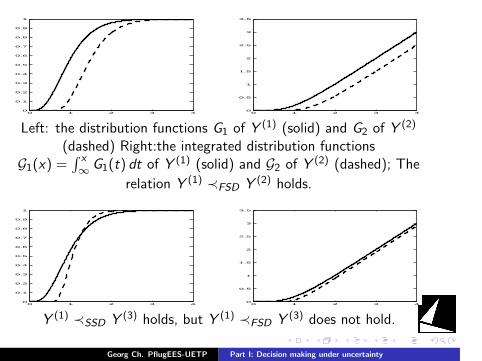
Left: the distribution functions G1 of Y (1) (solid) and G2 of Y (2)
(dashed) Right:the integrated distribution functionsG1(x) =
∫ x∞ G1(t) dt of Y (1) (solid) and G2 of Y (2) (dashed); The
relation Y (1) ≺FSD Y (2) holds.
0 1 2 3 40
0.1
0.2
0.3
0.4
0.5
0.6
0.7
0.8
0.9
1
0 1 2 3 40
0.5
1
1.5
2
2.5
3
3.5
Y (1) ≺SSD Y (3) holds, but Y (1) ≺FSD Y (3) does not hold.
Georg Ch. PflugEES-UETP Part I: Decision making under uncertainty
.
.
.
.
.
.
.
.
.
.
.
.
.
.
.
.
.
.
.
.
.
.
.
.
.
.
.
.
.
.
.
.
.
.
.
.
.
.
.
.
”Coherent risk measures”
Given an utility functional U , the mappings
R := −U
are called the associated risk functional/ risk measure.Coherent risk functionals are negative utility functionals which arepositively homogeneous in addition. (Artzner et al., 1999).
Georg Ch. PflugEES-UETP Part I: Decision making under uncertainty
.
.
.
.
.
.
.
.
.
.
.
.
.
.
.
.
.
.
.
.
.
.
.
.
.
.
.
.
.
.
.
.
.
.
.
.
.
.
.
.
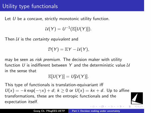
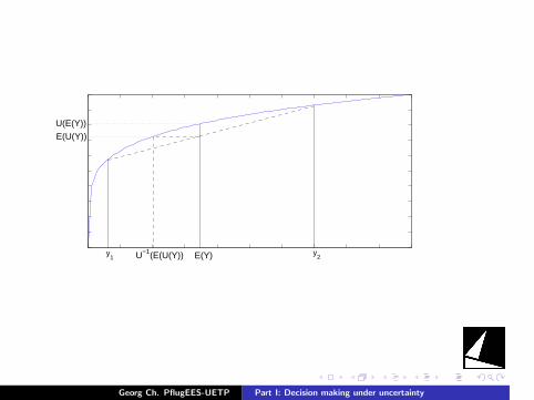
Utility type functionals
Let U be a concave, strictly monotonic utility function.
U(Y ) = U−1(E[U(Y )]).
Then U is the certainty equivalent and
D(Y ) = EY − U(Y ),
may be seen as risk premium. The decision maker with utilityfunction U is indifferent between Y and the deterministic value Uin the sense that
E[U(Y )] = U[U(Y )].
This type of functionals is translation-equivariant iffU(x) = −k exp(−γx) + d ; k ≥ 0 or U(x) = kx + d . Up to affinetransformations, these are the entropic functionals and theexpectation itself.
Georg Ch. PflugEES-UETP Part I: Decision making under uncertainty
.
.
.
.
.
.
.
.
.
.
.
.
.
.
.
.
.
.
.
.
.
.
.
.
.
.
.
.
.
.
.
.
.
.
.
.
.
.
.
.
U(E(Y))
y2y
1
E(U(Y))
U−1(E(U(Y)) E(Y)
Georg Ch. PflugEES-UETP Part I: Decision making under uncertainty
.
.
.
.
.
.
.
.
.
.
.
.
.
.
.
.
.
.
.
.
.
.
.
.
.
.
.
.
.
.
.
.
.
.
.
.
.
.
.
.
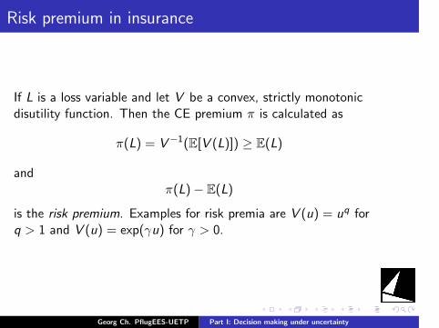
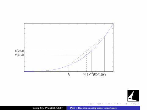
Risk premium in insurance
If L is a loss variable and let V be a convex, strictly monotonicdisutility function. Then the CE premium π is calculated as
π(L) = V−1(E[V (L)]) ≥ E(L)
andπ(L)− E(L)
is the risk premium. Examples for risk premia are V (u) = uq forq > 1 and V (u) = exp(γu) for γ > 0.
Georg Ch. PflugEES-UETP Part I: Decision making under uncertainty
.
.
.
.
.
.
.
.
.
.
.
.
.
.
.
.
.
.
.
.
.
.
.
.
.
.
.
.
.
.
.
.
.
.
.
.
.
.
.
.
l1
l2E(L) V−1(E(V(L)))
E(V(L))
V(E(L))
Georg Ch. PflugEES-UETP Part I: Decision making under uncertainty
.
.
.
.
.
.
.
.
.
.
.
.
.
.
.
.
.
.
.
.
.
.
.
.
.
.
.
.
.
.
.
.
.
.
.
.
.
.
.
.
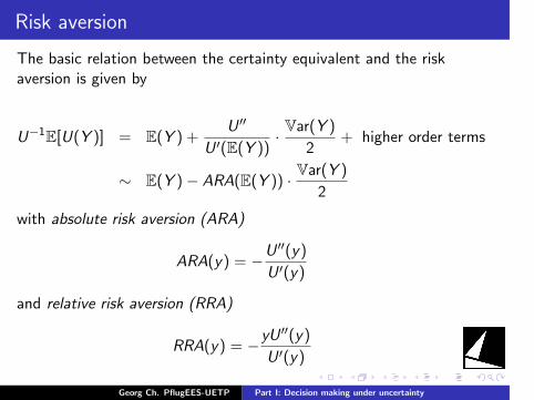
Risk aversion
The basic relation between the certainty equivalent and the riskaversion is given by
U−1E[U(Y )] = E(Y ) +U ′′
U ′(E(Y ))· Var(Y )
2+ higher order terms
∼ E(Y )− ARA(E(Y )) · Var(Y )
2
with absolute risk aversion (ARA)
ARA(y) = −U ′′(y)
U ′(y)
and relative risk aversion (RRA)
RRA(y) = −yU ′′(y)
U ′(y)
Georg Ch. PflugEES-UETP Part I: Decision making under uncertainty
.
.
.
.
.
.
.
.
.
.
.
.
.
.
.
.
.
.
.
.
.
.
.
.
.
.
.
.
.
.
.
.
.
.
.
.
.
.
.
.
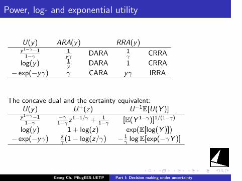
Power, log- and exponential utility
U(y) ARA(y) RRA(y)y1−γ−11−γ
1yγ DARA 1
γ CRRA
log(y) 1y DARA 1 CRRA
− exp(−yγ) γ CARA yγ IRRA
The concave dual and the certainty equivalent:U(y) U+(z) U−1E[U(Y )]y1−γ−11−γ
−γ1−γ z
1−1/γ + 11−γ [E(Y 1−γ)]1/(1−γ)
log(y) 1 + log(z) exp(E[log(Y )])− exp(−yγ) z
γ (1− log(z/γ) − 1γ logE[exp(−γY )]
Georg Ch. PflugEES-UETP Part I: Decision making under uncertainty
.
.
.
.
.
.
.
.
.
.
.
.
.
.
.
.
.
.
.
.
.
.
.
.
.
.
.
.
.
.
.
.
.
.
.
.
.
.
.
.
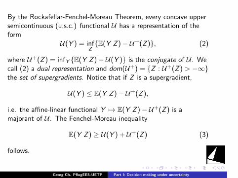
By the Rockafellar-Fenchel-Moreau Theorem, every concave uppersemicontinuous (u.s.c.) functional U has a representation of theform
U(Y ) = infZE(Y Z )− U+(Z ), (2)
where U+(Z ) = infY E(Y Z )− U(Y ) is the conjugate of U . Wecall (2) a dual representation and dom(U+) = Z : U+(Z ) > −∞the set of supergradients. Notice that if Z is a supergradient,
U(Y ) ≤ E(Y Z )− U+(Z ),
i.e. the affine-linear functional Y 7→ E(Y Z )− U+(Z ) is amajorant of U . The Fenchel-Moreau inequality
E(Y Z ) ≥ U(Y ) + U+(Z ) (3)
follows.
Georg Ch. PflugEES-UETP Part I: Decision making under uncertainty
.
.
.
.
.
.
.
.
.
.
.
.
.
.
.
.
.
.
.
.
.
.
.
.
.
.
.
.
.
.
.
.
.
.
.
.
.
.
.
.
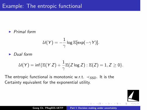
Example: The entropic functional
I Primal form
U(Y ) = −1
γlogE[exp(−γY )].
I Dual form
U(Y ) = infE(Y Z ) +1
γE(Z logZ ) : E(Z ) = 1,Z ≥ 0.
The entropic functional is monotonic w.r.t. ≺SSD . It is theCertainty equivalent for the exponential utility.
Georg Ch. PflugEES-UETP Part I: Decision making under uncertainty
.
.
.
.
.
.
.
.
.
.
.
.
.
.
.
.
.
.
.
.
.
.
.
.
.
.
.
.
.
.
.
.
.
.
.
.
.
.
.
.
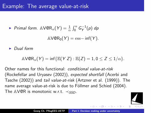
Example: The average value-at-risk
I Primal form. AV@Rα(Y ) = 1α
∫ α0 G−1
Y (p) dp
AV@R0(Y ) = ess− inf(Y ).
I Dual form
AV@Rα(Y ) = infE(Y Z ) : E(Z ) = 1, 0 ≤ Z ≤ 1/α.
Other names for this functional: conditional value-at-risk(Rockefellar and Uryasev (2002)), expected shortfall (Acerbi andTasche (2002)) and tail value-at-risk (Artzner et al. (1999)). Thename average value-at-risk is due to Follmer and Schied (2004).The AV@R is monotonic w.r.t. ≺SSD .
Georg Ch. PflugEES-UETP Part I: Decision making under uncertainty

.
.
.
.
.
.
.
.
.
.
.
.
.
.
.
.
.
.
.
.
.
.
.
.
.
.
.
.
.
.
.
.
.
.
.
.
.
.
.
.
Risk corrected expectation I
Let h be a nonnegative convex function on R with h(0) = 0. .
I Primal form. U(Y ) = EY − E[h(Y − EY )].
I Dual form. U(Y ) = infE(Y Z ) + Dh∗(Z ) : EZ = 1, whereDh∗(Z ) = infE[h∗(Z − a)] : a ∈ Randh∗(u) = supuv − h(v) : v ∈ R is the Fenchel conjugate of h.
For example h(u) = u2. However, for every δ > 0, there arerandom variables Y (1) and Y (2) such that Y (1) ≺FSD Y (2), butEY (1) − δVarY (1) > EY (2) − δVarY (2).
Georg Ch. PflugEES-UETP Part I: Decision making under uncertainty
.
.
.
.
.
.
.
.
.
.
.
.
.
.
.
.
.
.
.
.
.
.
.
.
.
.
.
.
.
.
.
.
.
.
.
.
.
.
.
.
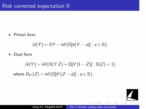
Risk corrected expectation II
I Primal form
U(Y ) = EY − infE[h(Y − a)] : a ∈ R.
I Dual form
U(Y ) = infE(Y Z ) + E[h∗(1− Z )] : E(Z ) = 1
where Dh∗(Z ) = infE[h∗(Z − a)] : a ∈ R.
Georg Ch. PflugEES-UETP Part I: Decision making under uncertainty
.
.
.
.
.
.
.
.
.
.
.
.
.
.
.
.
.
.
.
.
.
.
.
.
.
.
.
.
.
.
.
.
.
.
.
.
.
.
.
.
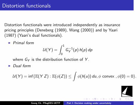
Distortion functionals
Distortion functionals were introduced independently as insurancepricing principles (Deneberg (1989), Wang (2000)) and by Yaari(1987) (Yaari’s dual functionals).
I Primal form
U(Y ) =
∫ 1
0G−1Y (p) h(p) dp
where GY is the distribution function of Y .
I Dual form
U(Y ) = infE(Y Z ) : E(ϕ(Z )) ≤∫
ϕ(h(u)) du, ϕ convex , ϕ(0) = 0.
Georg Ch. PflugEES-UETP Part I: Decision making under uncertainty
.
.
.
.
.
.
.
.
.
.
.
.
.
.
.
.
.
.
.
.
.
.
.
.
.
.
.
.
.
.
.
.
.
.
.
.
.
.
.
.
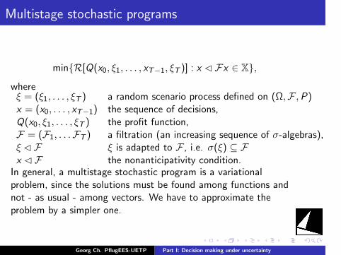
Multistage stochastic programs
minR[Q(x0, ξ1, . . . , xT−1, ξT )] : x Fx ∈ X,
whereξ = (ξ1, . . . , ξT ) a random scenario process defined on (Ω,F ,P)x = (x0, . . . , xT−1) the sequence of decisions,Q(x0, ξ1, . . . , ξT ) the profit function,F = (F1, . . .FT ) a filtration (an increasing sequence of σ-algebras),ξ F ξ is adapted to F , i.e. σ(ξ) ⊆ Fx F the nonanticipativity condition.
In general, a multistage stochastic program is a variationalproblem, since the solutions must be found among functions andnot - as usual - among vectors. We have to approximate theproblem by a simpler one.
Georg Ch. PflugEES-UETP Part I: Decision making under uncertainty
.
.
.
.
.
.
.
.
.
.
.
.
.
.
.
.
.
.
.
.
.
.
.
.
.
.
.
.
.
.
.
.
.
.
.
.
.
.
.
.
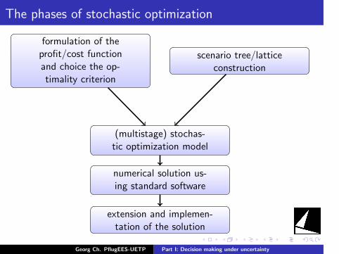
The phases of stochastic optimization
formulation of theprofit/cost functionand choice the op-timality criterion
scenario tree/latticeconstruction
(multistage) stochas-tic optimization model
numerical solution us-ing standard software
extension and implemen-tation of the solution
Georg Ch. PflugEES-UETP Part I: Decision making under uncertainty
.
.
.
.
.
.
.
.
.
.
.
.
.
.
.
.
.
.
.
.
.
.
.
.
.
.
.
.
.
.
.
.
.
.
.
.
.
.
.
.
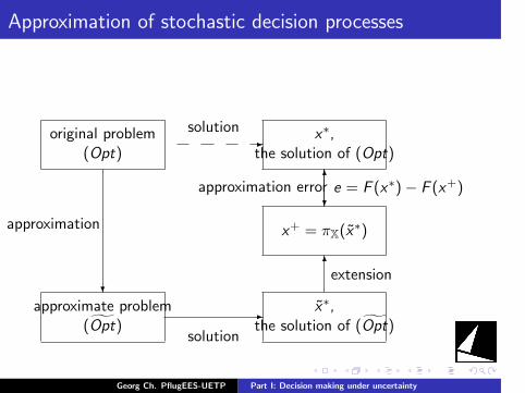
Approximation of stochastic decision processes
approximate problem(Opt)
original problem(Opt)
x∗,the solution of (Opt)
x+ = πX(x∗)
x∗,the solution of (Opt)
?
-
-
6
6
?
solution
solution
approximation
extension
approximation error e = F (x∗)− F (x+)
Georg Ch. PflugEES-UETP Part I: Decision making under uncertainty
.
.
.
.
.
.
.
.
.
.
.
.
.
.
.
.
.
.
.
.
.
.
.
.
.
.
.
.
.
.
.
.
.
.
.
.
.
.
.
.
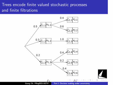
Trees encode finite valued stochastic processesand finite filtrations
7
1
@@@
@@@R
1
PPPPPPq
-
3
-QQQ
QQQs
ξ1,1
ξ1,2
ξ1,3
x1,1
x1,2
x1,3
ξ2,1
ξ2,2
ξ2,3
ξ2,4
ξ2,5
ξ2,6
x2,1
x2,2
x2,3
x2,4
x2,5
x2,6
0.5
0.3
0.4
0.6
1.0
0.20.4
0.2
0.4
ξ1 ξ2Georg Ch. PflugEES-UETP Part I: Decision making under uncertainty
.
.
.
.
.
.
.
.
.
.
.
.
.
.
.
.
.
.
.
.
.
.
.
.
.
.
.
.
.
.
.
.
.
.
.
.
.
.
.
.
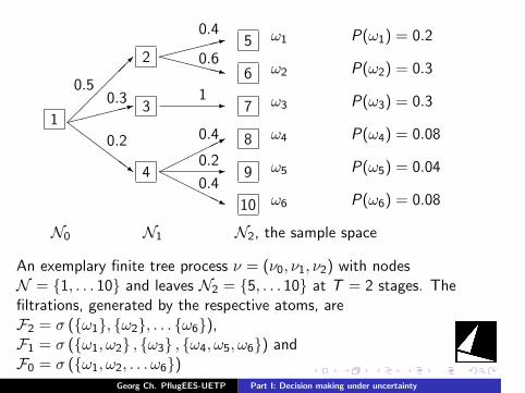
:0.4
5 ω1 P(ω1) = 0.2
XXXXXz0.6
6 ω2 P(ω2) = 0.3
-17 ω3 P(ω3) = 0.3
*0.4 8 ω4 P(ω4) = 0.08
-0.29 ω5 P(ω5) = 0.04HHHHHj
0.4
10 ω6 P(ω6) = 0.08
0.5
2
:0.3
3
ZZZ
ZZ~
0.2
4
1
N0 N1 N2, the sample space
An exemplary finite tree process ν = (ν0, ν1, ν2) with nodesN = 1, . . . 10 and leaves N2 = 5, . . . 10 at T = 2 stages. Thefiltrations, generated by the respective atoms, areF2 = σ (ω1, ω2, . . . ω6),F1 = σ (ω1, ω2 , ω3 , ω4, ω5, ω6) andF0 = σ (ω1, ω2, . . . ω6)
Georg Ch. PflugEES-UETP Part I: Decision making under uncertainty
.
.
.
.
.
.
.
.
.
.
.
.
.
.
.
.
.
.
.
.
.
.
.
.
.
.
.
.
.
.
.
.
.
.
.
.
.
.
.
.
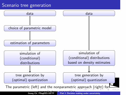
Scenario tree generation
data
choice of parametric model
estimation of parameters
simulation of(conditional)distributions
tree generation by(optimal) quantization
data
simulation of(conditional) distributionsbased on density estimates
tree generation by(optimal) quantization
The parametric (left) and the nonparametric approach (right) forscenario tree generation.Georg Ch. PflugEES-UETP Part I: Decision making under uncertainty
.
.
.
.
.
.
.
.
.
.
.
.
.
.
.
.
.
.
.
.
.
.
.
.
.
.
.
.
.
.
.
.
.
.
.
.
.
.
.
.
The approximation dilemma
The approximation should be coarse enough to allow an efficientnumerical solution but also fine enough to make the approximationerror small. It is therefore of fundamental interest to understandthe relation between the complexity and the approximation qualityof approximative models.
We quantify the approximation error by a new distance concept,the nested distance for scenario processes and the informationstructure.
Georg Ch. PflugEES-UETP Part I: Decision making under uncertainty
.
.
.
.
.
.
.
.
.
.
.
.
.
.
.
.
.
.
.
.
.
.
.
.
.
.
.
.
.
.
.
.
.
.
.
.
.
.
.
.
The Monge/Kantorovich/Wasserstein transportationdistance
d1(P1,P2) = sup|∫
f (u) dP1(u)−∫
f (u) dP2(u)| :
|f (u)− f (v)| ≤ ∥u − v∥Theorem (Kantorovich-Rubinstein). Dualization:
d1(P1,P2) = infE(∥X − Y ∥ : (X ,Y ) is a bivariate r.v. with
given marginal distributions P1 and P2.A generalization of the Kantorovich distance is the Wassersteindistance of order r
drr (P1,P2) = infE(∥X − Y ∥r : (X ,Y ) is a bivariate r.v. with
given marginal distributions P1 and P2.The infimum is attained. The bivariate distribution with marginalsP1 resp. P2 which is the minimizer is called the optimaltransportation plan.Georg Ch. PflugEES-UETP Part I: Decision making under uncertainty
.
.
.
.
.
.
.
.
.
.
.
.
.
.
.
.
.
.
.
.
.
.
.
.
.
.
.
.
.
.
.
.
.
.
.
.
.
.
.
.
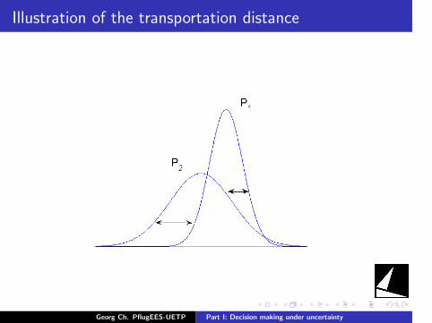
Illustration of the transportation distance
Georg Ch. PflugEES-UETP Part I: Decision making under uncertainty
.
.
.
.
.
.
.
.
.
.
.
.
.
.
.
.
.
.
.
.
.
.
.
.
.
.
.
.
.
.
.
.
.
.
.
.
.
.
.
.
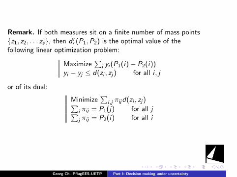
Remark. If both measures sit on a finite number of mass pointsz1, z2, . . . zs, then d r
r (P1,P2) is the optimal value of thefollowing linear optimization problem:
Maximize∑
i yi (P1(i)− P2(i))yi − yj ≤ d(zi , zj) for all i , j
or of its dual:
Minimize∑
i ,j πijd(zi , zj)∑i πij = P1(j) for all j∑j πij = P2(i) for all i
Georg Ch. PflugEES-UETP Part I: Decision making under uncertainty

.
.
.
.
.
.
.
.
.
.
.
.
.
.
.
.
.
.
.
.
.
.
.
.
.
.
.
.
.
.
.
.
.
.
.
.
.
.
.
.
Illustration: The Kantorovich distance as the solution ofa transportation problem
Georg Ch. PflugEES-UETP Part I: Decision making under uncertainty
.
.
.
.
.
.
.
.
.
.
.
.
.
.
.
.
.
.
.
.
.
.
.
.
.
.
.
.
.
.
.
.
.
.
.
.
.
.
.
.
Historical remarks
The distance d1 was introduced by Kantorovich in 1942 as adistance in general spaces. In 1948, he established the relation ofthis distance (in Rm) to the mass transportation problemformulated by Gaspard Monge in 1781 (Monge’s masstransportation problem). In 1969, L. N. Wasserstein –unaware ofthe work of Kantorovich – this distance for using it for convergenceresults of Markov processes and one year later R. L. Dobrushinused and generalized this distance and initiated the nameWasserstein distance. S. S. Vallander studied the special case ofmeasures in R1 in 1974 and this paper made the name Wassersteinmetric popular. Modern books have been written by Rachev andRuschendorf (1998) and Villani (2003).
Georg Ch. PflugEES-UETP Part I: Decision making under uncertainty
.
.
.
.
.
.
.
.
.
.
.
.
.
.
.
.
.
.
.
.
.
.
.
.
.
.
.
.
.
.
.
.
.
.
.
.
.
.
.
.
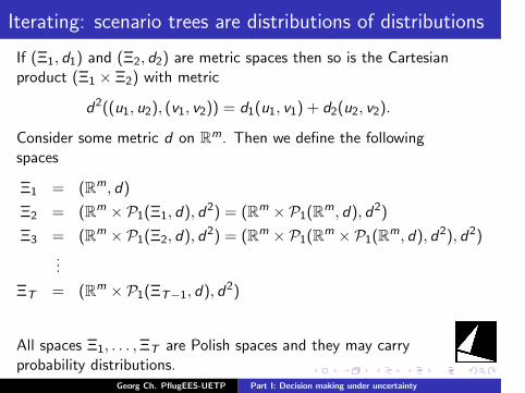
Iterating: scenario trees are distributions of distributions
If (Ξ1, d1) and (Ξ2, d2) are metric spaces then so is the Cartesianproduct (Ξ1 × Ξ2) with metric
d2((u1, u2), (v1, v2)) = d1(u1, v1) + d2(u2, v2).
Consider some metric d on Rm. Then we define the followingspaces
Ξ1 = (Rm, d)
Ξ2 = (Rm × P1(Ξ1, d), d2) = (Rm × P1(Rm, d), d2)
Ξ3 = (Rm × P1(Ξ2, d), d2) = (Rm × P1(Rm × P1(Rm, d), d2), d2)
...
ΞT = (Rm × P1(ΞT−1, d), d2)
All spaces Ξ1, . . . ,ΞT are Polish spaces and they may carryprobability distributions.
Georg Ch. PflugEES-UETP Part I: Decision making under uncertainty
.
.
.
.
.
.
.
.
.
.
.
.
.
.
.
.
.
.
.
.
.
.
.
.
.
.
.
.
.
.
.
.
.
.
.
.
.
.
.
.
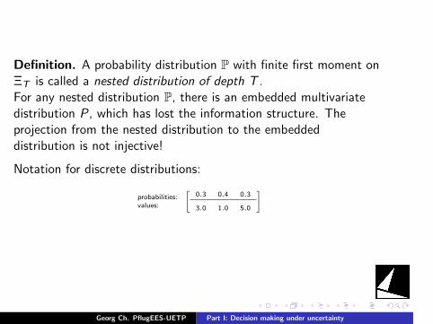
Definition. A probability distribution P with finite first moment onΞT is called a nested distribution of depth T .For any nested distribution P, there is an embedded multivariatedistribution P , which has lost the information structure. Theprojection from the nested distribution to the embeddeddistribution is not injective!
Notation for discrete distributions:
probabilities:values:
[0.3 0.4 0.3
3.0 1.0 5.0
]
Georg Ch. PflugEES-UETP Part I: Decision making under uncertainty
.
.
.
.
.
.
.
.
.
.
.
.
.
.
.
.
.
.
.
.
.
.
.
.
.
.
.
.
.
.
.
.
.
.
.
.
.
.
.
.
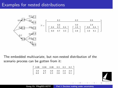
Examples for nested distributions
7
1
@@@R
1PPPq
-
3-
QQQs
2.4
3.0
3.0
5.1
1.0
2.8
3.3
4.7
6.0
0.5
0.3
0.4
0.6
1.0
0.20.4
0.2
0.4
P =
0.2 0.3 0.5
3.0 3.0 2.4[0.4 0.2 0.4
6.0 4.7 3.3
] [1.0
2.8
] [0.6 0.4
1.0 5.1
]
The embedded multivariate, but non-nested distribution of thescenario process can be gotten from it:
0.08 0.04 0.08 0.3 0.3 0.2
3.0 3.0 3.0 3.0 2.4 2.46.0 4.7 3.3 2.8 1.0 5.1
Georg Ch. PflugEES-UETP Part I: Decision making under uncertainty
.
.
.
.
.
.
.
.
.
.
.
.
.
.
.
.
.
.
.
.
.
.
.
.
.
.
.
.
.
.
.
.
.
.
.
.
.
.
.
.
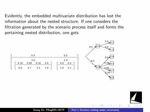
Evidently, the embedded multivariate distribution has lost theinformation about the nested structure. If one considers thefiltration generated by the scenario process itself and forms thepertaining nested distribution, one gets
0.5 0.5
3.0 2.4[0.16 0.08 0.16 0.6
6.0 4.7 3.3 2.8
] [0.6 0.4
1.0 5.1
]
@@@R
1PPPq
1PPPq@@@R
2.4
3.0
5.1
1.0
2.8
3.3
4.7
6.0
0.5
0.5
0.4
0.6
0.6
0.16
0.08
0.16
Georg Ch. PflugEES-UETP Part I: Decision making under uncertainty
.
.
.
.
.
.
.
.
.
.
.
.
.
.
.
.
.
.
.
.
.
.
.
.
.
.
.
.
.
.
.
.
.
.
.
.
.
.
.
.
Distances between nested distributions
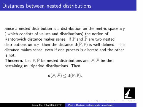
Since a nested distribution is a distribution on the metric space ΞT
( which consists of values and distributions) the notion ofKantorovich distance makes sense. If P and P are two nesteddistributions on ΞT , then the distance dl(P,P) is well defined. Thisdistance makes sense, even if one process is discrete and the otheris not.Theorem. Let P, P be nested distributions and P , P be thepertaining multiperiod distributions. Then
d(P, P) ≤ dl(P, P).
Georg Ch. PflugEES-UETP Part I: Decision making under uncertainty
.
.
.
.
.
.
.
.
.
.
.
.
.
.
.
.
.
.
.
.
.
.
.
.
.
.
.
.
.
.
.
.
.
.
.
.
.
.
.
.
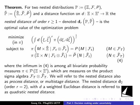
Theorem. For two nested distributions P := (Ξ,F ,P),P :=
(Ξ, F , P
)and a distance function on d : Ξ× Ξ′ → R the
nested distance of order r ≥ 1 – denoted dlr(P, P
)– is the
optimal value of the optimization problem
minimize(in π)
(∫d(ξ, ξ
)rπ(dξ, dξ
)) 1r
subject to π(M × Ξ | Ft ⊗ Ft
)= P (M | Ft) (M ∈ FT )
π(Ξ× N | Ft ⊗ Ft
)= P
(N | Ft
) (N ∈ FT
)(4)
where the infimum in (4) is among all bivariate probabilitymeasures π ∈ P (Ξ× Ξ′), which are measures on the productsigma algebra FT ⊗ FT . We will refer to the nested distance alsoas process distance, or multistage distance. The nested distance dl2(order r = 2), with d a weighted Euclidean distance is referred toas quadratic nested distance.
Georg Ch. PflugEES-UETP Part I: Decision making under uncertainty
.
.
.
.
.
.
.
.
.
.
.
.
.
.
.
.
.
.
.
.
.
.
.
.
.
.
.
.
.
.
.
.
.
.
.
.
.
.
.
.
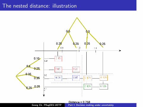
The nested distance: illustration
Georg Ch. PflugEES-UETP Part I: Decision making under uncertainty
.
.
.
.
.
.
.
.
.
.
.
.
.
.
.
.
.
.
.
.
.
.
.
.
.
.
.
.
.
.
.
.
.
.
.
.
.
.
.
.
Georg Ch. PflugEES-UETP Part I: Decision making under uncertainty
.
.
.
.
.
.
.
.
.
.
.
.
.
.
.
.
.
.
.
.
.
.
.
.
.
.
.
.
.
.
.
.
.
.
.
.
.
.
.
.
What we have achieved
I The nested distribution contains both the information aboutthe scenario values and the available information (thefiltration) in a version-independent way.
I The nested distance quantifies the approximation errorbetween continuous and discrete models (or large and smalldiscrete models). It is the natural extension of theKantorovich distance in two-stage models (see shortly).
I By minimaxing over nested balls, solutions which are robustagainst model ambiguity can be found (second part of thelecture).
Georg Ch. PflugEES-UETP Part I: Decision making under uncertainty
.
.
.
.
.
.
.
.
.
.
.
.
.
.
.
.
.
.
.
.
.
.
.
.
.
.
.
.
.
.
.
.
.
.
.
.
.
.
.
.
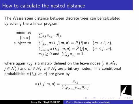
How to calculate the nested distance
The Wasserstein distance between discrete trees can be calculatedby solving the a linear program
minimize(in π)
∑i ,j πi ,j · d r
i ,j
subject to∑
j≻n π (i , j |m, n) = P (i |m) (m ≺ i , n),∑i≻m π (i , j |m, n) = P (j | n) (n ≺ j , m),
πi ,j ≥ 0 and∑
i ,j πi ,j = 1,
where again πi ,j is a matrix defined on the leave nodes (i ∈ NT ,j ∈ N ′
T ) and m ∈ Nt , n ∈ N ′t are arbitrary nodes. The conditional
probabilities π (i , j |m, n) are given by
π (i , j |m, n) =πi ,j∑
i ′≻m, j ′≻n πi ′,j ′.
Georg Ch. PflugEES-UETP Part I: Decision making under uncertainty
.
.
.
.
.
.
.
.
.
.
.
.
.
.
.
.
.
.
.
.
.
.
.
.
.
.
.
.
.
.
.
.
.
.
.
.
.
.
.
.
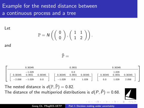
Example for the nested distance betweena continuous process and a tree
Let
P = N
((00
),
(1 11 2
)).
and
P =
0.30345 0.3931 0.30345
−1.029 0.0 1.029[0.30345 0.3931 0.30345
−2.058 −1.029 0.0
] [0.30345 0.3931 0.30345
−1.029 0.0 1.029
] [0.30345 0.3931 0.30345
0.0 1.029 2.058
]
The nested distance is d(P, P) = 0.82.The distance of the multiperiod distributions is d(P , P) = 0.68.
Georg Ch. PflugEES-UETP Part I: Decision making under uncertainty
.
.
.
.
.
.
.
.
.
.
.
.
.
.
.
.
.
.
.
.
.
.
.
.
.
.
.
.
.
.
.
.
.
.
.
.
.
.
.
.
−3−2
−10
12
3
−3
−2
−1
0
1
2
3
0
0.05
0.1
0.15
−3−2
−10
12
3
−3
−2
−1
0
1
2
3
0
0.05
0.1
0.15
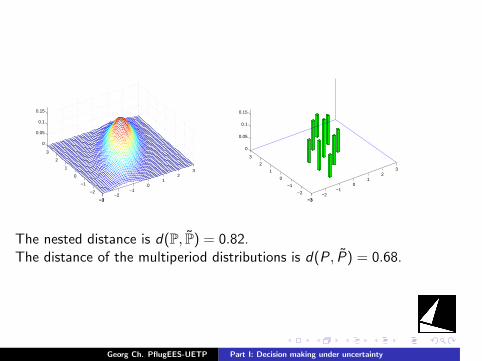
The nested distance is d(P, P) = 0.82.The distance of the multiperiod distributions is d(P , P) = 0.68.
Georg Ch. PflugEES-UETP Part I: Decision making under uncertainty
.
.
.
.
.
.
.
.
.
.
.
.
.
.
.
.
.
.
.
.
.
.
.
.
.
.
.
.
.
.
.
.
.
.
.
.
.
.
.
.
−3−2
−10
12
3
−3
−2
−1
0
1
2
3
0
0.05
0.1
0.15
−3−2
−10
12
3
−3
−2
−1
0
1
2
3
0
0.05
0.1
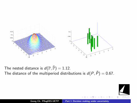
The nested distance is d(P, P) = 1.12.The distance of the multiperiod distributions is d(P , P) = 0.67.
Georg Ch. PflugEES-UETP Part I: Decision making under uncertainty
.
.
.
.
.
.
.
.
.
.
.
.
.
.
.
.
.
.
.
.
.
.
.
.
.
.
.
.
.
.
.
.
.
.
.
.
.
.
.
.
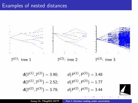
Examples of nested distances
P(1): tree 1 P(2): tree 2 P(3): tree 3
dl(P(1),P(2)) = 3.90; d(P(1),P(2)) = 3.48
dl(P(1),P(3)) = 2.52; d(P(1),P(3)) = 1.77
dl(P(2),P(3)) = 3.79; d(P(2),P(3)) = 3.44
Georg Ch. PflugEES-UETP Part I: Decision making under uncertainty
.
.
.
.
.
.
.
.
.
.
.
.
.
.
.
.
.
.
.
.
.
.
.
.
.
.
.
.
.
.
.
.
.
.
.
.
.
.
.
.
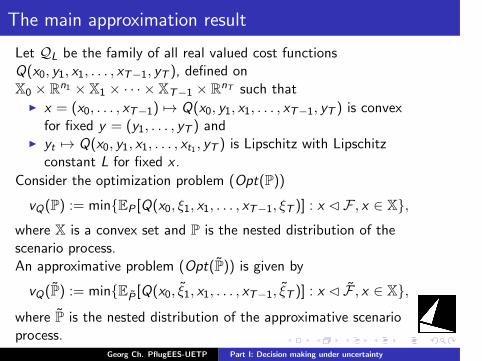
The main approximation result
Let QL be the family of all real valued cost functionsQ(x0, y1, x1, . . . , xT−1, yT ), defined onX0 × Rn1 × X1 × · · · × XT−1 × RnT such that
I x = (x0, . . . , xT−1) 7→ Q(x0, y1, x1, . . . , xT−1, yT ) is convexfor fixed y = (y1, . . . , yT ) and
I yt 7→ Q(x0, y1, x1, . . . , xt1 , yT ) is Lipschitz with Lipschitzconstant L for fixed x .
Consider the optimization problem (Opt(P))
vQ(P) := minEP [Q(x0, ξ1, x1, . . . , xT−1, ξT )] : x F , x ∈ X,where X is a convex set and P is the nested distribution of thescenario process.An approximative problem (Opt(P)) is given by
vQ(P) := minEP [Q(x0, ξ1, x1, . . . , xT−1, ξT )] : x F , x ∈ X,
where P is the nested distribution of the approximative scenarioprocess.
Georg Ch. PflugEES-UETP Part I: Decision making under uncertainty
.
.
.
.
.
.
.
.
.
.
.
.
.
.
.
.
.
.
.
.
.
.
.
.
.
.
.
.
.
.
.
.
.
.
.
.
.
.
.
.
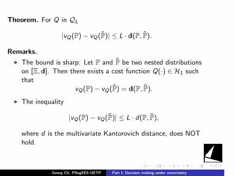
Theorem. For Q in QL
|vQ(P)− vQ(P)| ≤ L · dl(P, P).
Remarks.
I The bound is sharp: Let P and P be two nested distributionson [Ξ, dl]. Then there exists a cost function Q(·) ∈ H1 suchthat
vQ(P)− vQ(P) = dl(P, P).
I The inequality
|vQ(P)− vQ(P)| ≤ L · d(P, P),
where d is the multivariate Kantorovich distance, does NOThold.
Georg Ch. PflugEES-UETP Part I: Decision making under uncertainty
.
.
.
.
.
.
.
.
.
.
.
.
.
.
.
.
.
.
.
.
.
.
.
.
.
.
.
.
.
.
.
.
.
.
.
.
.
.
.
.
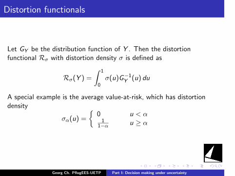
Distortion functionals
Let GY be the distribution function of Y . Then the distortionfunctional Rσ with distortion density σ is defined as
Rσ(Y ) =
∫ 1
0σ(u)G−1
Y (u) du
A special example is the average value-at-risk, which has distortiondensity
σα(u) =
0 u < α1
1−α u ≥ α
Georg Ch. PflugEES-UETP Part I: Decision making under uncertainty
.
.
.
.
.
.
.
.
.
.
.
.
.
.
.
.
.
.
.
.
.
.
.
.
.
.
.
.
.
.
.
.
.
.
.
.
.
.
.
.
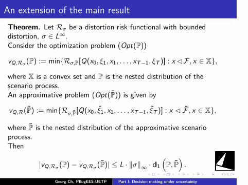
An extension of the main result
Theorem. Let Rσ be a distortion risk functional with boundeddistortion, σ ∈ L∞.Consider the optimization problem (Opt(P))
vQ,Rσ(P) := minRσ,P[Q(x0, ξ1, x1, . . . , xT−1, ξT )] : xF , x ∈ X,
where X is a convex set and P is the nested distribution of thescenario process.An approximative problem (Opt(P)) is given by
vQ,R(P) := minRσ,P[Q(x0, ξ1, x1, . . . , xT−1, ξT )] : x F , x ∈ X,
where P is the nested distribution of the approximative scenarioprocess.Then
|vQ,Rσ(P)− vQ,Rσ(P)| ≤ L · ∥σ∥∞ · dl1(P, P
).
Georg Ch. PflugEES-UETP Part I: Decision making under uncertainty
.
.
.
.
.
.
.
.
.
.
.
.
.
.
.
.
.
.
.
.
.
.
.
.
.
.
.
.
.
.
.
.
.
.
.
.
.
.
.
.
Optimal discretizations
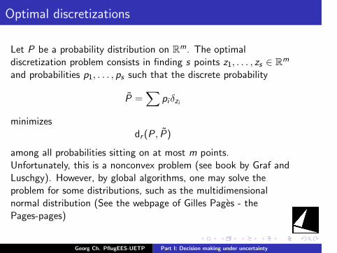
Let P be a probability distribution on Rm. The optimaldiscretization problem consists in finding s points z1, . . . , zs ∈ Rm
and probabilities p1, . . . , ps such that the discrete probability
P =∑
piδzi
minimizesdr (P, P)
among all probabilities sitting on at most m points.Unfortunately, this is a nonconvex problem (see book by Graf andLuschgy). However, by global algorithms, one may solve theproblem for some distributions, such as the multidimensionalnormal distribution (See the webpage of Gilles Pages - thePages-pages)
Georg Ch. PflugEES-UETP Part I: Decision making under uncertainty
.
.
.
.
.
.
.
.
.
.
.
.
.
.
.
.
.
.
.
.
.
.
.
.
.
.
.
.
.
.
.
.
.
.
.
.
.
.
.
.
Scenario Tree Generation
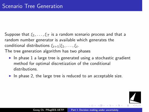
Suppose that ξ1, . . . , ξT is a random scenario process and that arandom number generator is available which generates theconditional distributions ξt+1|ξ1, . . . , ξt .The tree generation algorithm has two phases
I In phase 1 a large tree is generated using a stochastic gradientmethod for optimal discretization of the conditionaldistributions.
I In phase 2, the large tree is reduced to an acceptable size.
Georg Ch. PflugEES-UETP Part I: Decision making under uncertainty
.
.
.
.
.
.
.
.
.
.
.
.
.
.
.
.
.
.
.
.
.
.
.
.
.
.
.
.
.
.
.
.
.
.
.
.
.
.
.
.
Facility location by stochastic gradient search
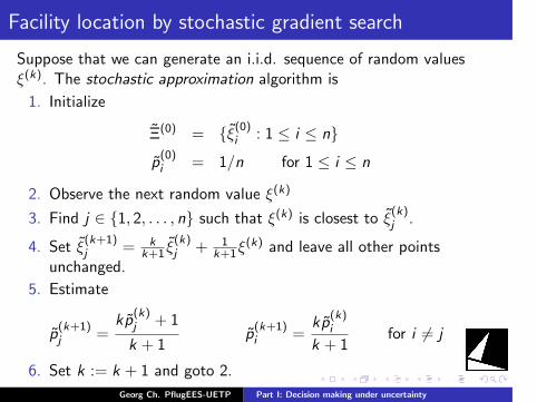
Suppose that we can generate an i.i.d. sequence of random valuesξ(k). The stochastic approximation algorithm is
1. Initialize
Ξ(0) = ξ(0)i : 1 ≤ i ≤ n
p(0)i = 1/n for 1 ≤ i ≤ n
2. Observe the next random value ξ(k)
3. Find j ∈ 1, 2, . . . , n such that ξ(k) is closest to ξ(k)j .
4. Set ξ(k+1)j = k
k+1 ξ(k)j + 1
k+1ξ(k) and leave all other points
unchanged.
5. Estimate
p(k+1)j =
kp(k)j + 1
k + 1p(k+1)i =
kp(k)i
k + 1for i = j
6. Set k := k + 1 and goto 2.
Georg Ch. PflugEES-UETP Part I: Decision making under uncertainty
.
.
.
.
.
.
.
.
.
.
.
.
.
.
.
.
.
.
.
.
.
.
.
.
.
.
.
.
.
.
.
.
.
.
.
.
.
.
.
.
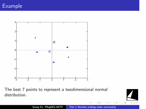
Example
The best 7 points to represent a twodimensional normaldistribution.
Georg Ch. PflugEES-UETP Part I: Decision making under uncertainty
.
.
.
.
.
.
.
.
.
.
.
.
.
.
.
.
.
.
.
.
.
.
.
.
.
.
.
.
.
.
.
.
.
.
.
.
.
.
.
.
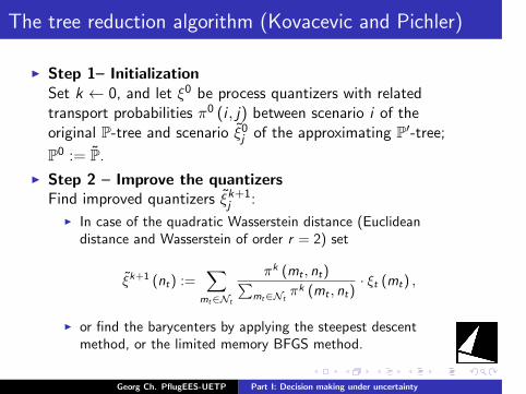
The tree reduction algorithm (Kovacevic and Pichler)
I Step 1– InitializationSet k ← 0, and let ξ0 be process quantizers with relatedtransport probabilities π0 (i , j) between scenario i of theoriginal P-tree and scenario ξ0j of the approximating P′-tree;
P0 := P.I Step 2 – Improve the quantizers
Find improved quantizers ξk+1j :
I In case of the quadratic Wasserstein distance (Euclideandistance and Wasserstein of order r = 2) set
ξk+1 (nt) :=∑
mt∈Nt
πk (mt , nt)∑mt∈Nt
πk (mt , nt)· ξt (mt) ,
I or find the barycenters by applying the steepest descentmethod, or the limited memory BFGS method.
Georg Ch. PflugEES-UETP Part I: Decision making under uncertainty
.
.
.
.
.
.
.
.
.
.
.
.
.
.
.
.
.
.
.
.
.
.
.
.
.
.
.
.
.
.
.
.
.
.
.
.
.
.
.
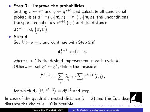
.
I Step 3 – Improve the probabilitiesSetting π ← πk and q ← qk+1 and calculate all conditionalprobabilities πk+1 (·, ·|m, n) = π∗ (·, ·|m, n), the unconditionaltransport probabilities πk+1 (·, ·) and the distance
dlk+1r = dlr
(P, P
).
I Step 4Set k ← k + 1 and continue with Step 2 if
dlk+1r < dlkr − ε,
where ε > 0 is the desired improvement in each cycle k.Otherwise, set ξ∗ ← ξk , define the measure
Pk+1 :=∑j
δξk+1j·∑i
πk+1 (i , j) ,
for which dlr(P,Pk+1
)= dlk+1
r and stop.
In case of the quadratic nested distance (r = 2) and the Euclideandistance the choice ε = 0 is possible.
Georg Ch. PflugEES-UETP Part I: Decision making under uncertainty
.
.
.
.
.
.
.
.
.
.
.
.
.
.
.
.
.
.
.
.
.
.
.
.
.
.
.
.
.
.
.
.
.
.
.
.
.
.
.
.
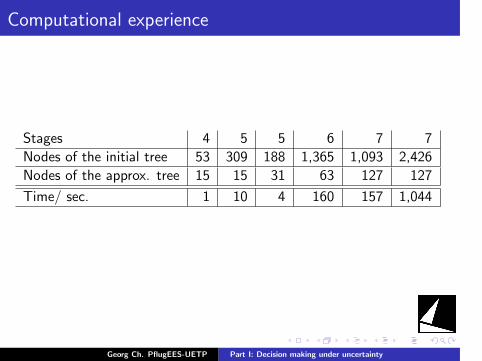
Computational experience
Stages 4 5 5 6 7 7
Nodes of the initial tree 53 309 188 1,365 1,093 2,426
Nodes of the approx. tree 15 15 31 63 127 127
Time/ sec. 1 10 4 160 157 1,044
Georg Ch. PflugEES-UETP Part I: Decision making under uncertainty
.
.
.
.
.
.
.
.
.
.
.
.
.
.
.
.
.
.
.
.
.
.
.
.
.
.
.
.
.
.
.
.
.
.
.
.
.
.
.
.
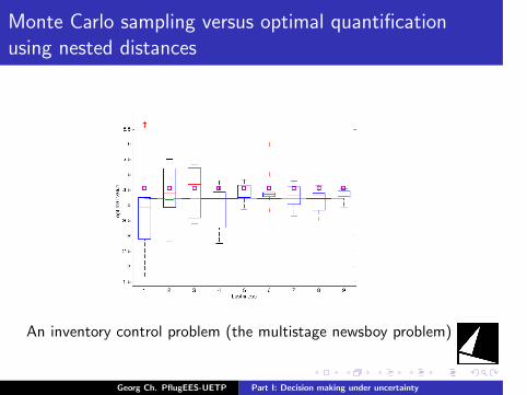
Monte Carlo sampling versus optimal quantificationusing nested distances
An inventory control problem (the multistage newsboy problem)
Georg Ch. PflugEES-UETP Part I: Decision making under uncertainty

.
.
.
.
.
.
.
.
.
.
.
.
.
.
.
.
.
.
.
.
.
.
.
.
.
.
.
.
.
.
.
.
.
.
.
.
.
.
.
.
Approximation at work
Reducing the nested distance by making the tree bushier.
Georg Ch. PflugEES-UETP Part I: Decision making under uncertainty
.
.
.
.
.
.
.
.
.
.
.
.
.
.
.
.
.
.
.
.
.
.
.
.
.
.
.
.
.
.
.
.
.
.
.
.
.
.
.
.
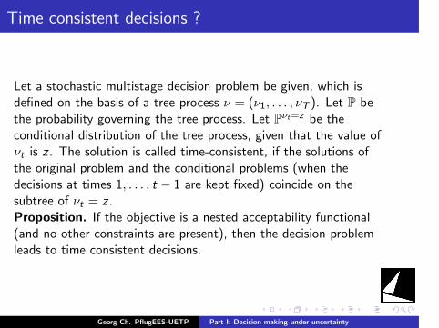
Time consistent decisions ?
Let a stochastic multistage decision problem be given, which isdefined on the basis of a tree process ν = (ν1, . . . , νT ). Let P bethe probability governing the tree process. Let Pνt=z be theconditional distribution of the tree process, given that the value ofνt is z . The solution is called time-consistent, if the solutions ofthe original problem and the conditional problems (when thedecisions at times 1, . . . , t − 1 are kept fixed) coincide on thesubtree of νt = z .Proposition. If the objective is a nested acceptability functional(and no other constraints are present), then the decision problemleads to time consistent decisions.
Georg Ch. PflugEES-UETP Part I: Decision making under uncertainty
.
.
.
.
.
.
.
.
.
.
.
.
.
.
.
.
.
.
.
.
.
.
.
.
.
.
.
.
.
.
.
.
.
.
.
.
.
.
.
.
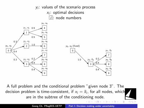
yi : values of the scenario processxi : optimal decisionsi : node numbers
7
1
@@
@@R
1PPPPq
-
3
-Q
QQQs
0.3
0.4
0.3
0.5
0.5
1.0
0.2
0.4
0.4
0
y0, x0
1
y1, x1
2
y2, x2
3
y3, x3
4
y4, x4
5
y5, x5
6
y6, x6
7
y7, x7
8
y8, x8
9
y9, x9
@@@@R
3
-QQQQs
1.0 0.2
0.4
0.4
0
y0, x0 (fixed)
3
y3, x3
7
y7, x7
8
y8, x8
9
y9, x9
A full problem and the conditional problem ”given node 3”. Thedecision problem is time-consistent, if xi = xi , for all nodes, which
are in the subtree of the conditioning node.
Georg Ch. PflugEES-UETP Part I: Decision making under uncertainty
.
.
.
.
.
.
.
.
.
.
.
.
.
.
.
.
.
.
.
.
.
.
.
.
.
.
.
.
.
.
.
.
.
.
.
.
.
.
.
.
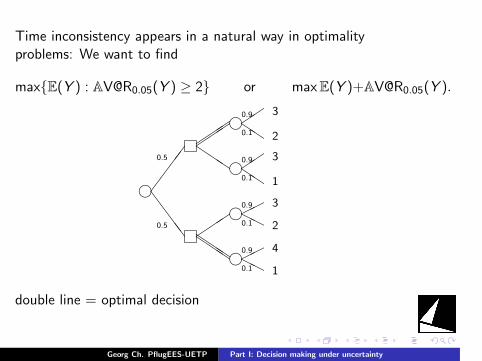
Time inconsistency appears in a natural way in optimalityproblems: We want to find
maxE(Y ) : [email protected](Y ) ≥ 2 or maxE(Y )[email protected](Y ).
h
hhS
SSS
QQQ HH
HH0.5
0.9
0.1
0.9
0.1
3
2
4
1
hh
QQQ
0.5
0.9
0.1
0.9
0.1
3
2
3
1
QQQ
double line = optimal decision
Georg Ch. PflugEES-UETP Part I: Decision making under uncertainty
.
.
.
.
.
.
.
.
.
.
.
.
.
.
.
.
.
.
.
.
.
.
.
.
.
.
.
.
.
.
.
.
.
.
.
.
.
.
.
.
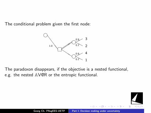
The conditional problem given the first node:
h
hhS
SSS
QQQ HH
HH1.0
0.9
0.1
0.9
0.1
3
2
4
1
The paradoxon disappears, if the objective is a nested functional,e.g. the nested AV@R or the entropic functional.
Georg Ch. PflugEES-UETP Part I: Decision making under uncertainty
.
.
.
.
.
.
.
.
.
.
.
.
.
.
.
.
.
.
.
.
.
.
.
.
.
.
.
.
.
.
.
.
.
.
.
.
.
.
.
.
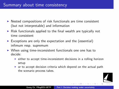
Summary about time consistency
I Nested compositions of risk functionals are time consistent(but not interpretable) and information
I Risk functionals applied to the final wealth are typically nottime consistent
I Exceptions are only the expectation and the (essential)infimum resp. supremum
I When using time-inconsistent functionals one one has todecide:
I either to accept time-inconsistent decisions in a rolling horizonsetup
I or to accept decision criteria which depend on the actual paththe scenario process takes.
Georg Ch. PflugEES-UETP Part I: Decision making under uncertainty

.
.
.
.
.
.
.
.
.
.
.
.
.
.
.
.
.
.
.
.
.
.
.
.
.
.
.
.
.
.
.
.
.
.
.
.
.
.
.
.
Part II: Pricing of energy contracts
Georg Ch. Pflug
July 3, 2016
Georg Ch. Pflug Part II: Pricing of energy contracts
.
.
.
.
.
.
.
.
.
.
.
.
.
.
.
.
.
.
.
.
.
.
.
.
.
.
.
.
.
.
.
.
.
.
.
.
.
.
.
.
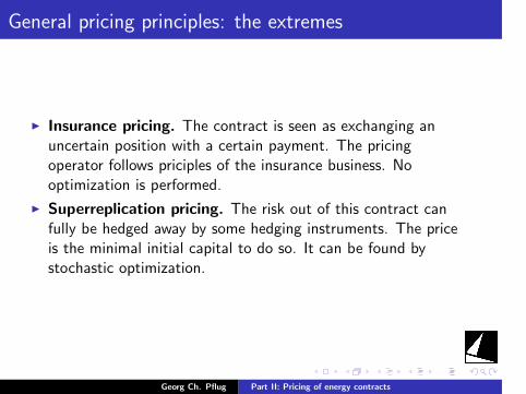
General pricing principles: the extremes
I Insurance pricing. The contract is seen as exchanging anuncertain position with a certain payment. The pricingoperator follows priciples of the insurance business. Nooptimization is performed.
I Superreplication pricing. The risk out of this contract canfully be hedged away by some hedging instruments. The priceis the minimal initial capital to do so. It can be found bystochastic optimization.
Georg Ch. Pflug Part II: Pricing of energy contracts
.
.
.
.
.
.
.
.
.
.
.
.
.
.
.
.
.
.
.
.
.
.
.
.
.
.
.
.
.
.
.
.
.
.
.
.
.
.
.
.
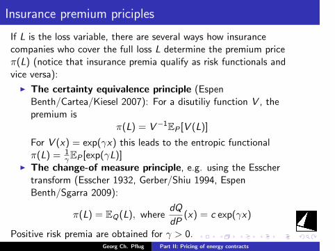
Insurance premium priciples
If L is the loss variable, there are several ways how insurancecompanies who cover the full loss L determine the premium priceπ(L) (notice that insurance premia qualify as risk functionals andvice versa):
I The certainty equivalence principle (EspenBenth/Cartea/Kiesel 2007): For a disutiliy function V , thepremium is
π(L) = V−1EP [V (L)]
For V (x) = exp(γx) this leads to the entropic functionalπ(L) = 1
γEP [exp(γL)]I The change-of measure principle, e.g. using the Esscher
transform (Esscher 1932, Gerber/Shiu 1994, EspenBenth/Sgarra 2009):
π(L) = EQ(L), wheredQ
dP(x) = c exp(γx)
Positive risk premia are obtained for γ > 0.Georg Ch. Pflug Part II: Pricing of energy contracts
.
.
.
.
.
.
.
.
.
.
.
.
.
.
.
.
.
.
.
.
.
.
.
.
.
.
.
.
.
.
.
.
.
.
.
.
.
.
.
.
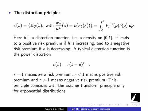
I The distortion priciple:
π(L) = EQ(L), withdQ
dP(x) = h(FL(x)) =
∫ 1
0F−1L (p)h(p) dp
Here h is a distortion function, i.e. a density on [0,1]. It leadsto a positive risk premium if h is increasing, and to a negativerisk premium if h is decreasing. A typical distortion function isthe power distortion
h(u) = r(1− u)r−1.
r = 1 means zero risk premium, r < 1 means positive riskpremium and r > 1 means negative risk premium. Thisprinciple coincides with the Esscher transform principle onlyfor exponential distributions.
Georg Ch. Pflug Part II: Pricing of energy contracts
.
.
.
.
.
.
.
.
.
.
.
.
.
.
.
.
.
.
.
.
.
.
.
.
.
.
.
.
.
.
.
.
.
.
.
.
.
.
.
.
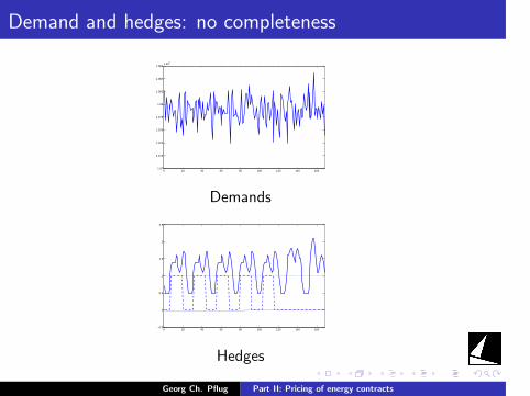
Demand and hedges: no completeness
0 20 40 60 80 100 120 140 1601.07
1.072
1.074
1.076
1.078
1.08
1.082
1.084
1.086x 10
5
Demands
0 20 40 60 80 100 120 140 160−0.5
0
0.5
1
1.5
2
2.5
Hedges
Georg Ch. Pflug Part II: Pricing of energy contracts
.
.
.
.
.
.
.
.
.
.
.
.
.
.
.
.
.
.
.
.
.
.
.
.
.
.
.
.
.
.
.
.
.
.
.
.
.
.
.
.
Pricing between the extremes
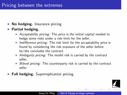
I No hedging. Insurance pricing
I Partial hedging.I Acceptability pricing: The price is the initial capital needed to
hedge some risks under a risk limit for the seller.I Indifference pricing: The risk limit for the accaptability price is
found by considering the risk exposure of the seller beforehe/she concludes the contract.
I Ambiguity pricing: The model risk is carried by the contractseller.
I Bilevel pricing: The counterparty risk is carried by the contractseller.
I Full hedging. Superreplication pricing
Georg Ch. Pflug Part II: Pricing of energy contracts
.
.
.
.
.
.
.
.
.
.
.
.
.
.
.
.
.
.
.
.
.
.
.
.
.
.
.
.
.
.
.
.
.
.
.
.
.
.
.
.
Pricing between the extremes
I No hedging. Insurance pricingI Partial hedging.
I Acceptability pricing: The price is the initial capital needed tohedge some risks under a risk limit for the seller.
I Indifference pricing: The risk limit for the accaptability price isfound by considering the risk exposure of the seller beforehe/she concludes the contract.
I Ambiguity pricing: The model risk is carried by the contractseller.
I Bilevel pricing: The counterparty risk is carried by the contractseller.
I Full hedging. Superreplication pricing
Georg Ch. Pflug Part II: Pricing of energy contracts
.
.
.
.
.
.
.
.
.
.
.
.
.
.
.
.
.
.
.
.
.
.
.
.
.
.
.
.
.
.
.
.
.
.
.
.
.
.
.
.
Pricing Financial Contracts
I Bid -price: The price of a contract is acceptable for th buyeronly if there is no better investment, i.e. no alternativestrategy, which for a smaller initial installment would give atleast the same outpayments as the given contract.
I Ask-price: The price of the contract is acceptable for theseller only if there is no contract, which pays more at thebeginning and has lower or equal liabilities at later stages.
By a duality argument, one sees that the ask-price is always smallerthan the bid-price, if there is no arbitrage. In complete markets,they are even equal. Under arbitrage possibilities, the ask-price islarger than the bid-price. The fundamental theorem says that amarket is arbitrage free iff there is a probability measure such thatthe properly discounted price process of the assets is a martingale.
Georg Ch. Pflug Part II: Pricing of energy contracts
.
.
.
.
.
.
.
.
.
.
.
.
.
.
.
.
.
.
.
.
.
.
.
.
.
.
.
.
.
.
.
.
.
.
.
.
.
.
.
.
Replication for energy contracts
There is a fundamental difference between pricing in financialmarkets and pricing in energy markets: While the set of feasibletrading strategies is considered to be the same for the seller and forthe buyer, it is different in energy markets: The seller has a muchlarger spectrum of possible actions, he/she may use own energyproduction, buy energy futures and trade on the wholesale markets,the buyer typically has no access to these possibilities, maybe forthe exception of access to the spot markets. For this reason, theseller may determine the upper price by including all his/her assetsin a replication model and may offer this price to the buyer.
Georg Ch. Pflug Part II: Pricing of energy contracts

.
.
.
.
.
.
.
.
.
.
.
.
.
.
.
.
.
.
.
.
.
.
.
.
.
.
.
.
.
.
.
.
.
.
.
.
.
.
.
.
Notations:Ct payments (cash-inflow) to the contract sellerJ = 0, . . . , J energy forms (electricity: j = 0, gas, oil, water)Set,j spot prices
0 ≤ xet,j ≤ xej storage and constraints (for electricity xej = 0)
x ft,0 cash with an interest yield of rf > 0
y et = (y et,0, . . . , yt,J) amount of energy bought or sold
dt,j ≥ 0 random inflows (solar, wind, water)zet,ij production of energy i out of energy j
z t,ij ≤ zet,ij ≤ zt,ij production limit
ηij efficiencies of conversionγt,ij cost factorsS ft,i financial assets paying cash flows C f
t,i
Dt(t, j) delivery of energy j in period [t, t + 1) in MWh to the contract seller
Georg Ch. Pflug Part II: Pricing of energy contracts
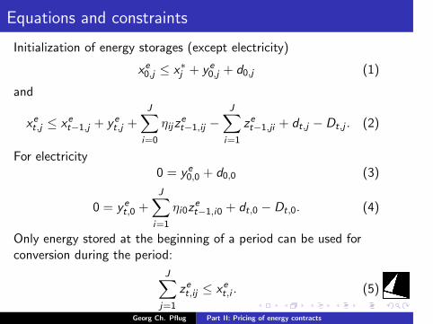
.
.
.
.
.
.
.
.
.
.
.
.
.
.
.
.
.
.
.
.
.
.
.
.
.
.
.
.
.
.
.
.
.
.
.
.
.
.
.
.
Equations and constraints
Initialization of energy storages (except electricity)
xe0,j ≤ x∗j + y e0,j + d0,j (1)
and
xet,j ≤ xet−1,j + y et,j +J∑
i=0
ηijzet−1,ij −
J∑i=1
zet−1,ji + dt,j − Dt,j . (2)
For electricity0 = y e0,0 + d0,0 (3)
0 = y et,0 +J∑
i=1
ηi0zet−1,i0 + dt,0 − Dt,0. (4)
Only energy stored at the beginning of a period can be used forconversion during the period:
J∑j=1
zet,ij ≤ xet,i . (5)
Georg Ch. Pflug Part II: Pricing of energy contracts
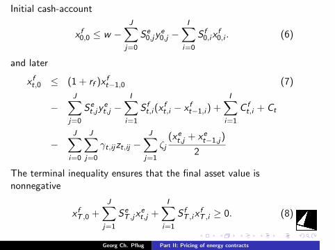
.
.
.
.
.
.
.
.
.
.
.
.
.
.
.
.
.
.
.
.
.
.
.
.
.
.
.
.
.
.
.
.
.
.
.
.
.
.
.
.
Initial cash-account
x f0,0 ≤ w −J∑
j=0
Se0,jy
e0,j −
I∑i=0
S f0,ix
f0,i . (6)
and later
x ft,0 ≤ (1 + rf )xft−1,0 (7)
−J∑
j=0
Set,jy
et,j −
I∑i=1
S ft,i (x
ft,i − x ft−1,i ) +
I∑i=1
C ft,i + Ct
−J∑
i=0
J∑j=0
γt,ijzt,ij −J∑
j=1
ζj(xet,j + xet−1,j)
2
The terminal inequality ensures that the final asset value isnonnegative
x fT ,0 +J∑
j=1
SeT ,jx
et,j +
I∑i=1
S fT ,ix
fT ,i ≥ 0. (8)
Georg Ch. Pflug Part II: Pricing of energy contracts
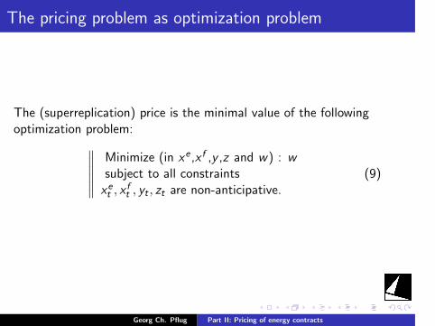
.
.
.
.
.
.
.
.
.
.
.
.
.
.
.
.
.
.
.
.
.
.
.
.
.
.
.
.
.
.
.
.
.
.
.
.
.
.
.
.
The pricing problem as optimization problem
The (superreplication) price is the minimal value of the followingoptimization problem:∥∥∥∥∥∥
Minimize (in xe ,x f ,y ,z and w) : wsubject to all constraintsxet , x
ft , yt , zt are non-anticipative.
(9)
Georg Ch. Pflug Part II: Pricing of energy contracts
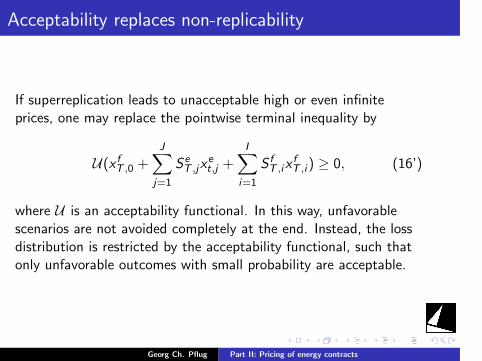
.
.
.
.
.
.
.
.
.
.
.
.
.
.
.
.
.
.
.
.
.
.
.
.
.
.
.
.
.
.
.
.
.
.
.
.
.
.
.
.
Acceptability replaces non-replicability
If superreplication leads to unacceptable high or even infiniteprices, one may replace the pointwise terminal inequality by
U(x fT ,0 +J∑
j=1
SeT ,jx
et,j +
I∑i=1
S fT ,ix
fT ,i ) ≥ 0, (16’)
where U is an acceptability functional. In this way, unfavorablescenarios are not avoided completely at the end. Instead, the lossdistribution is restricted by the acceptability functional, such thatonly unfavorable outcomes with small probability are acceptable.
Georg Ch. Pflug Part II: Pricing of energy contracts
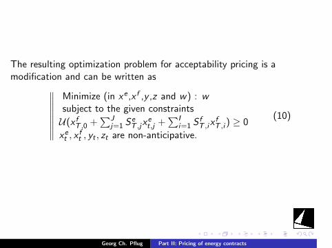
.
.
.
.
.
.
.
.
.
.
.
.
.
.
.
.
.
.
.
.
.
.
.
.
.
.
.
.
.
.
.
.
.
.
.
.
.
.
.
.
The resulting optimization problem for acceptability pricing is amodification and can be written as∥∥∥∥∥∥∥∥
Minimize (in xe ,x f ,y ,z and w) : wsubject to the given constraints
U(x fT ,0 +∑J
j=1 SeT ,jx
et,j +
∑Ii=1 S
fT ,ix
fT ,i ) ≥ 0
xet , xft , yt , zt are non-anticipative.
(10)
Georg Ch. Pflug Part II: Pricing of energy contracts
.
.
.
.
.
.
.
.
.
.
.
.
.
.
.
.
.
.
.
.
.
.
.
.
.
.
.
.
.
.
.
.
.
.
.
.
.
.
.
.
An example
We consider a planning horizon of one year (52 weeks). Electricityspot prices are modeled by geometric Brownian motion with jumps(GBMJ), estimated from EEX Phelix hourly electricity prices(hourly, 09/2008-12/2011, Bloomberg). The pricing model wasreformulated and solved on a stochastic tree, generated from theGBMJ model.The hedging opportunities are represented by four futurescontracts, related to the quarters of the year, i.e. each of thefutures delivers a constant amount of electric energy during one ofthe quarters.By solving the stochastic optimization problem withAV@R-objective, the acceptability price is calculated for a puretrader meaning that only wholesale base quarter future contractscan be used for hedging for different values of theAV@R-parameter α.
Georg Ch. Pflug Part II: Pricing of energy contracts
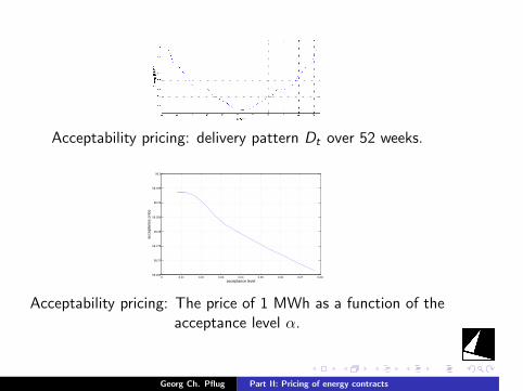
.
.
.
.
.
.
.
.
.
.
.
.
.
.
.
.
.
.
.
.
.
.
.
.
.
.
.
.
.
.
.
.
.
.
.
.
.
.
.
.
Acceptability pricing: delivery pattern Dt over 52 weeks.
0 0.01 0.02 0.03 0.04 0.05 0.06 0.07 0.0858.265
58.27
58.275
58.28
58.285
58.29
58.295
58.3
acceptance level
acce
ptan
ce p
rice
Acceptability pricing: The price of 1 MWh as a function of theacceptance level α.
Georg Ch. Pflug Part II: Pricing of energy contracts
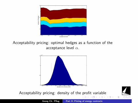
.
.
.
.
.
.
.
.
.
.
.
.
.
.
.
.
.
.
.
.
.
.
.
.
.
.
.
.
.
.
.
.
.
.
.
.
.
.
.
.
0.01 0.02 0.03 0.04 0.05 0.06 0.070
0.5
1
1.5
2
2.5
acceptance levelam
ount
of h
edge
s
Acceptability pricing: optimal hedges as a function of theacceptance level α.
−400 −200 0 200 400 600 800 1000 1200 1400 16000
0.5
1
1.5x 10
−3
density of the random profit
Acceptability pricing: density of the profit variable
Georg Ch. Pflug Part II: Pricing of energy contracts
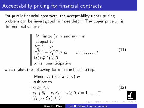
.
.
.
.
.
.
.
.
.
.
.
.
.
.
.
.
.
.
.
.
.
.
.
.
.
.
.
.
.
.
.
.
.
.
.
.
.
.
.
.
Acceptability pricing for financial contracts
For purely financial contracts, the acceptability upper pricingproblem can be investigated in more detail: The upper price πu isthe minimal value of∥∥∥∥∥∥∥∥∥∥∥∥
Minimize (in x and w) : wsubject toY w ,x0 = w
Y w ,xt− − Y w ,x
t ≥ ct t = 1, . . . ,TU(Y w ,x
T ) ≥ 0xt is nonanticipative
(11)
which takes the following form in the linear setup:∥∥∥∥∥∥∥∥∥∥Minimize (in x and w) wsubject tox0 S0 ≤ 0xt−1 St − xt St − ct ≥ 0; t = 1, . . . ,TUT (xT ST ) ≥ 0
(12)
Georg Ch. Pflug Part II: Pricing of energy contracts
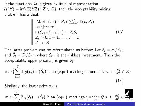
.
.
.
.
.
.
.
.
.
.
.
.
.
.
.
.
.
.
.
.
.
.
.
.
.
.
.
.
.
.
.
.
.
.
.
.
.
.
.
.
If the functional U is given by its dual representationU(Y ) = infE(YZ ) : Z ∈ Z, then the acceptability pricingproblem has a dual:∥∥∥∥∥∥∥∥∥∥
Maximize (in Zt)∑T
t=1 E(ct Zt)subject toE(St+1Zt+1|Ft) = ZtStZt ≥ 0; t = 1, . . . ,T − 1ZT ∈ Z
(13)
The latter problem can be reformulated as before: Let ct = ct/St,0and St = St/St,0, where St,0 is the riskless investment. Then theacceptability upper price πu is given by
maxT∑t=1
EQ(ct) : (St) is an (equ.) martingale under Q s. t. dQdP ∈ Z
(14)Similarly, the lower price πℓ is
minT∑t=1
EQ(ct) : (St) is an (equ.) martingale under Q s. t. dQdP ∈ Z
(15)Georg Ch. Pflug Part II: Pricing of energy contracts
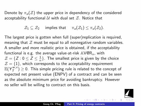
.
.
.
.
.
.
.
.
.
.
.
.
.
.
.
.
.
.
.
.
.
.
.
.
.
.
.
.
.
.
.
.
.
.
.
.
.
.
.
.
Denote by πu(Z) the upper price in dependency of the consideredacceptability functional U with dual set Z. Notice that
Z1 ⊆ Z2 implies that πu(Z1) ≤ πu(Z2).
The largest price is gotten when full (super)replication is required,meaning that Z must be equal to all nonnegative random variables.A smaller and more realistic price is obtained, if the acceptabilityfunctional is e.g. the average value-at-risk AV@Rα, withZ = Z : 0 ≤ Z ≤ 1
α. The smallest price is given by the choiceZ = 1, which corresponds to the acceptability requirementE(Y w ,x
T ) ≥ 0. This simple pricing rule is related to the concept ofexpected net present value (ENPV) of a contract and can be seenas the absolute minimum price for avoiding bankruptcy. Howeverno seller will be willing to contract on this basis.
Georg Ch. Pflug Part II: Pricing of energy contracts
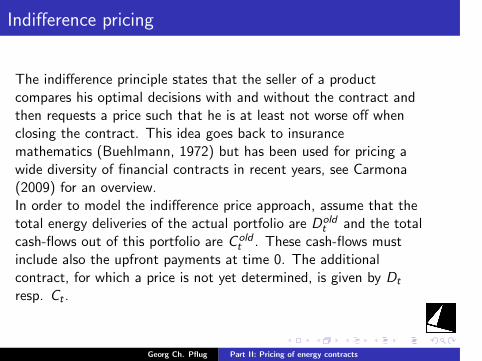
.
.
.
.
.
.
.
.
.
.
.
.
.
.
.
.
.
.
.
.
.
.
.
.
.
.
.
.
.
.
.
.
.
.
.
.
.
.
.
.
Indifference pricing
The indifference principle states that the seller of a productcompares his optimal decisions with and without the contract andthen requests a price such that he is at least not worse off whenclosing the contract. This idea goes back to insurancemathematics (Buehlmann, 1972) but has been used for pricing awide diversity of financial contracts in recent years, see Carmona(2009) for an overview.In order to model the indifference price approach, assume that thetotal energy deliveries of the actual portfolio are Dold
t and the totalcash-flows out of this portfolio are C old
t . These cash-flows mustinclude also the upfront payments at time 0. The additionalcontract, for which a price is not yet determined, is given by Dt
resp. Ct .
Georg Ch. Pflug Part II: Pricing of energy contracts
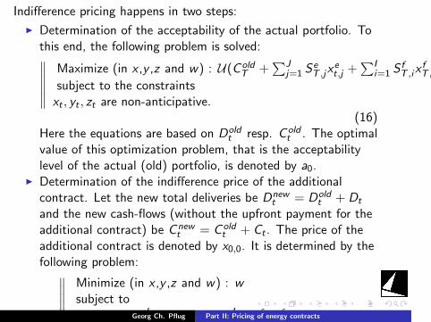
.
.
.
.
.
.
.
.
.
.
.
.
.
.
.
.
.
.
.
.
.
.
.
.
.
.
.
.
.
.
.
.
.
.
.
.
.
.
.
.
Indifference pricing happens in two steps:
I Determination of the acceptability of the actual portfolio. Tothis end, the following problem is solved:∥∥∥∥∥∥
Maximize (in x ,y ,z and w) : U(C oldT +
∑Jj=1 S
eT ,jx
et,j +
∑Ii=1 S
fT ,ix
fT ,i )
subject to the constraintsxt , yt , zt are non-anticipative.
(16)Here the equations are based on Dold
t resp. C oldt . The optimal
value of this optimization problem, that is the acceptabilitylevel of the actual (old) portfolio, is denoted by a0.
I Determination of the indifference price of the additionalcontract. Let the new total deliveries be Dnew
t = Doldt + Dt
and the new cash-flows (without the upfront payment for theadditional contract) be Cnew
t = C oldt + Ct . The price of the
additional contract is denoted by x0,0. It is determined by thefollowing problem:∥∥∥∥∥∥∥∥∥∥
Minimize (in x ,y ,z and w) : wsubject to
U(CnewT +
∑Jj=1 S
eT ,jx
et,j +
∑Ii=1 S
fT ,ix
fT ,i ) ≥ a0
and the constraintsxt , yt , zt are non-anticipative .
(17)
Of course, here the equations are based on Dnewt resp. Cnew
t .
Georg Ch. Pflug Part II: Pricing of energy contracts

.
.
.
.
.
.
.
.
.
.
.
.
.
.
.
.
.
.
.
.
.
.
.
.
.
.
.
.
.
.
.
.
.
.
.
.
.
.
.
.
Example
Consider an electricity producer, who has available a singlecombined cycle plant that is able to use both, oil and gas. Themachine has maximum power production of 410 MW andefficiencies of 0.575 (gas) and 0.57 (oil). Both fuels can be storedup to some amount (1.5 · 106 MWh) at storage costs 0.2Euro/MWh/h. We do not consider futures contracts in this setup,hence hedging is possible only by buying fuel at appropriate pointsin time. Again we use electricity prices and weekly decision periods.We valuate a simple delivery contract, which binds the producer tosupply a fixed amount of energy, the contract size in MWh, duringeach stage of the planning problem. The producer is free to buyand store fuel, and to produce electric energy for the contract andalso for selling it at the spot market. The value of the contract perMWh contains variable operating costs. From this we calculate acontract value per MWh that also includes an amount of coveragefor fixed cost, which is proportional to the mean workload of theproduction unit during the planning horizon.
Georg Ch. Pflug Part II: Pricing of energy contracts
.
.
.
.
.
.
.
.
.
.
.
.
.
.
.
.
.
.
.
.
.
.
.
.
.
.
.
.
.
.
.
.
.
.
.
.
.
.
.
.
Within this setup we compare the superhedging approach toindifference pricing. Superhedging is possible for a producer, if thecontract size does not exceed the capacity of the combined cycleturbine. For indifference pricing, we use the average value-at-riskat level α = 0.05 as the related acceptability functional.As described above, superhedging leads to contractual deliveries,but does not account for alternative usages of the machine,whereas indifference pricing does. This is the reason, why thesuperhedging price might be considered as too low in this case.Superhedging and indifference pricing also show different amountsof fixed cost, because the related strategies use non-contractualelectricity production at different levels.
Georg Ch. Pflug Part II: Pricing of energy contracts
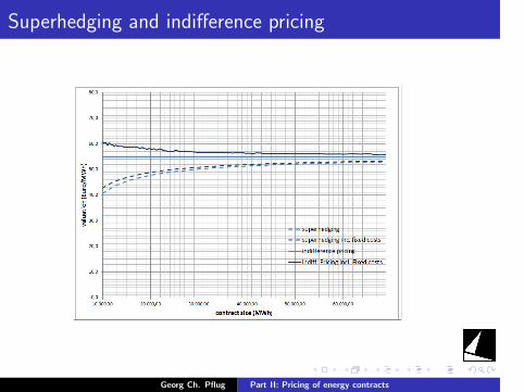
.
.
.
.
.
.
.
.
.
.
.
.
.
.
.
.
.
.
.
.
.
.
.
.
.
.
.
.
.
.
.
.
.
.
.
.
.
.
.
.
Superhedging and indifference pricing
Georg Ch. Pflug Part II: Pricing of energy contracts
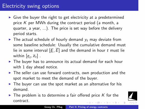
.
.
.
.
.
.
.
.
.
.
.
.
.
.
.
.
.
.
.
.
.
.
.
.
.
.
.
.
.
.
.
.
.
.
.
.
.
.
.
.
Electricity swing options
I Give the buyer the right to get electricity at a predeterminedprice K per MWh during the contract period (a month, aquarter, a year, ...). The price is set way before the deliveryperiod starts.
I The actual schedule of hourly demand yt may deviate fromsome baseline schedule: Usually the cumulative demand mustlie in some interval [E ,E ] and the demand in hour t must liewithin [et , et ] .
I The buyer has to announce its actual demand for each hourwith 1 day ahead notice.
I The seller can use forward contracts, own production and thespot market to meet the demand of the buyer.
I The buyer can use the spot market as an alternative for hisdemand.
I The problem is to determine a fair offered price K for thecontract.
Georg Ch. Pflug Part II: Pricing of energy contracts
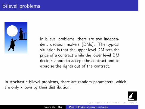
.
.
.
.
.
.
.
.
.
.
.
.
.
.
.
.
.
.
.
.
.
.
.
.
.
.
.
.
.
.
.
.
.
.
.
.
.
.
.
.
Bilevel problems
In bilevel problems, there are two indepen-dent decision makers (DMs): The typicalsituation is that the upper level DM sets theprice of a contract while the lower level DMdecides about to accept the contract and toexercise the rights out of the contract.
In stochastic bilevel problems, there are random parameters, whichare only known by their distribution.
Georg Ch. Pflug Part II: Pricing of energy contracts
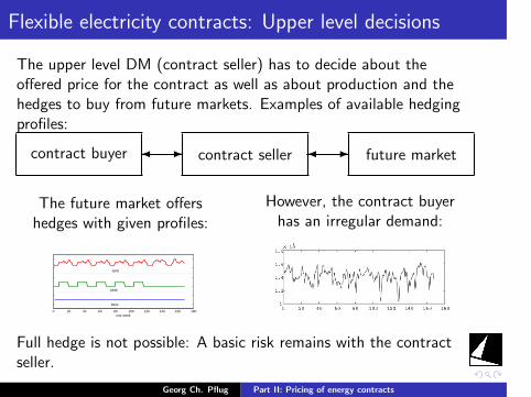
.
.
.
.
.
.
.
.
.
.
.
.
.
.
.
.
.
.
.
.
.
.
.
.
.
.
.
.
.
.
.
.
.
.
.
.
.
.
.
.
Flexible electricity contracts: Upper level decisions
The upper level DM (contract seller) has to decide about theoffered price for the contract as well as about production and thehedges to buy from future markets. Examples of available hedgingprofiles:
contract buyer contract seller future market- -
The future market offershedges with given profiles:
0 20 40 60 80 100 120 140 160 180one week
peak
base
GH0
However, the contract buyerhas an irregular demand:
Full hedge is not possible: A basic risk remains with the contractseller.
Georg Ch. Pflug Part II: Pricing of energy contracts
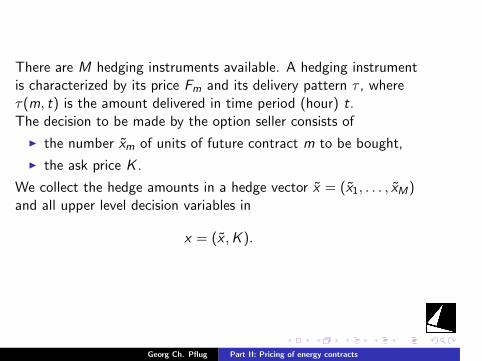
.
.
.
.
.
.
.
.
.
.
.
.
.
.
.
.
.
.
.
.
.
.
.
.
.
.
.
.
.
.
.
.
.
.
.
.
.
.
.
.
There are M hedging instruments available. A hedging instrumentis characterized by its price Fm and its delivery pattern τ , whereτ(m, t) is the amount delivered in time period (hour) t.The decision to be made by the option seller consists of
I the number xm of units of future contract m to be bought,
I the ask price K .
We collect the hedge amounts in a hedge vector x = (x1, . . . , xM)and all upper level decision variables in
x = (x ,K ).
Georg Ch. Pflug Part II: Pricing of energy contracts
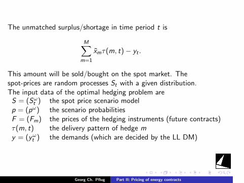
.
.
.
.
.
.
.
.
.
.
.
.
.
.
.
.
.
.
.
.
.
.
.
.
.
.
.
.
.
.
.
.
.
.
.
.
.
.
.
.
The unmatched surplus/shortage in time period t is
M∑m=1
xmτ(m, t)− yt .
This amount will be sold/bought on the spot market. Thespot-prices are random processes St with a given distribution.The input data of the optimal hedging problem areS = (Sω
t ) the spot price scenario modelp = (pω) the scenario probabilitiesF = (Fm) the prices of the hedging instruments (future contracts)τ(m, t) the delivery pattern of hedge my = (yωt ) the demands (which are decided by the LL DM)
Georg Ch. Pflug Part II: Pricing of energy contracts
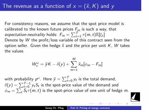
.
.
.
.
.
.
.
.
.
.
.
.
.
.
.
.
.
.
.
.
.
.
.
.
.
.
.
.
.
.
.
.
.
.
.
.
.
.
.
.
The revenue as a function of x = (x ,K ) and y
For consistency reasons, we assume that the spot price model iscalibrated to the known future prices Fm is such a way, thatexpectation-neutrality holds: Fm =
∑Tt=1 τ(m, t)E[ξt ]
Denote by W the profit/loss variable of this contract seen from theoption seller. Given the hedge x and the price per unit K , W takesthe values
W ωx = yK − δ(y) +
M∑m=1
xm[ϕm − Fm]
with probability pω. Here y =∑T
t=0 yt is the total demand,
δ(y) =∑T−1
t=0 ytSt is the spot-price value of the demand andϕm =
∑t Stτ(m, t) is the spot-price value of one unit of hedge m.
Georg Ch. Pflug Part II: Pricing of energy contracts
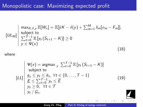
.
.
.
.
.
.
.
.
.
.
.
.
.
.
.
.
.
.
.
.
.
.
.
.
.
.
.
.
.
.
.
.
.
.
.
.
.
.
.
.
Monopolistic case: Maximizing expected profit
[ULM ]
∣∣∣∣∣∣∣∣maxK ,x ,y E[Wx ] = E[yK − δ(y) +
∑Mm=1 xm[ϕm − Fm]].
subject to∑T−1t=0 E [yt (St+1 − K )] ≥ 0
y ∈ Ψ(x)(18)
where
[LL]
∣∣∣∣∣∣∣∣∣∣∣∣∣
Ψ(x) = argmax y
∑T−1t=0 E [yt (St+1 − K )]
subject toet ≤ yt ≤ et , ∀t ∈ 0, . . . ,T − 1E ≤
∑T−1t=0 yt ≤ E
yt ≥ 0, ∀t ∈ Tyt Gt ,
(19)
Georg Ch. Pflug Part II: Pricing of energy contracts
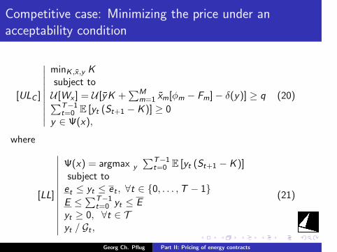
.
.
.
.
.
.
.
.
.
.
.
.
.
.
.
.
.
.
.
.
.
.
.
.
.
.
.
.
.
.
.
.
.
.
.
.
.
.
.
.
Competitive case: Minimizing the price under anacceptability condition
[ULC ]
∣∣∣∣∣∣∣∣∣∣
minK ,x ,y Ksubject to
U [Wx ] = U [yK +∑M
m=1 xm[ϕm − Fm]− δ(y)] ≥ q∑T−1t=0 E [yt (St+1 − K )] ≥ 0
y ∈ Ψ(x),
(20)
where
[LL]
∣∣∣∣∣∣∣∣∣∣∣∣∣
Ψ(x) = argmax y
∑T−1t=0 E [yt (St+1 − K )]
subject toet ≤ yt ≤ et , ∀t ∈ 0, . . . ,T − 1E ≤
∑T−1t=0 yt ≤ E
yt ≥ 0, ∀t ∈ Tyt Gt ,
(21)
Georg Ch. Pflug Part II: Pricing of energy contracts
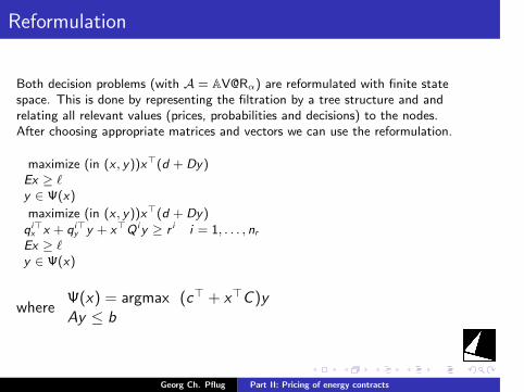
.
.
.
.
.
.
.
.
.
.
.
.
.
.
.
.
.
.
.
.
.
.
.
.
.
.
.
.
.
.
.
.
.
.
.
.
.
.
.
.
Reformulation
Both decision problems (with A = AV@Rα) are reformulated with finite statespace. This is done by representing the filtration by a tree structure and andrelating all relevant values (prices, probabilities and decisions) to the nodes.After choosing appropriate matrices and vectors we can use the reformulation.
maximize (in (x , y))x⊤(d + Dy)Ex ≥ ℓy ∈ Ψ(x)
maximize (in (x , y))x⊤(d + Dy)qi⊤x x + qi⊤
y y + x⊤Q iy ≥ r i i = 1, . . . , nrEx ≥ ℓy ∈ Ψ(x)
whereΨ(x) = argmax (c⊤ + x⊤C )yAy ≤ b
Georg Ch. Pflug Part II: Pricing of energy contracts
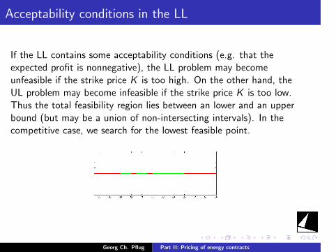
.
.
.
.
.
.
.
.
.
.
.
.
.
.
.
.
.
.
.
.
.
.
.
.
.
.
.
.
.
.
.
.
.
.
.
.
.
.
.
.
Acceptability conditions in the LL
If the LL contains some acceptability conditions (e.g. that theexpected profit is nonnegative), the LL problem may becomeunfeasible if the strike price K is too high. On the other hand, theUL problem may become infeasible if the strike price K is too low.Thus the total feasibility region lies between an lower and an upperbound (but may be a union of non-intersecting intervals). In thecompetitive case, we search for the lowest feasible point.
Georg Ch. Pflug Part II: Pricing of energy contracts
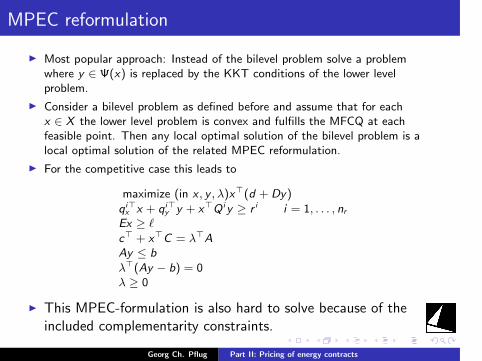
.
.
.
.
.
.
.
.
.
.
.
.
.
.
.
.
.
.
.
.
.
.
.
.
.
.
.
.
.
.
.
.
.
.
.
.
.
.
.
.
MPEC reformulation
I Most popular approach: Instead of the bilevel problem solve a problemwhere y ∈ Ψ(x) is replaced by the KKT conditions of the lower levelproblem.
I Consider a bilevel problem as defined before and assume that for eachx ∈ X the lower level problem is convex and fulfills the MFCQ at eachfeasible point. Then any local optimal solution of the bilevel problem is alocal optimal solution of the related MPEC reformulation.
I For the competitive case this leads to
maximize (in x , y , λ)x⊤(d + Dy)qi⊤x x + qi⊤
y y + x⊤Q iy ≥ r i i = 1, . . . , nrEx ≥ ℓ
c⊤ + x⊤C = λ⊤AAy ≤ bλ⊤(Ay − b) = 0λ ≥ 0
I This MPEC-formulation is also hard to solve because of theincluded complementarity constraints.
Georg Ch. Pflug Part II: Pricing of energy contracts
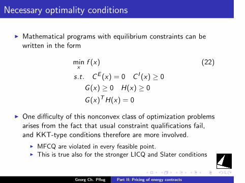
.
.
.
.
.
.
.
.
.
.
.
.
.
.
.
.
.
.
.
.
.
.
.
.
.
.
.
.
.
.
.
.
.
.
.
.
.
.
.
.
Necessary optimality conditions
I Mathematical programs with equilibrium constraints can bewritten in the form
minx
f (x) (22)
s.t. CE (x) = 0 C I (x) ≥ 0
G (x) ≥ 0 H(x) ≥ 0
G (x)TH(x) = 0
I One difficulty of this nonconvex class of optimization problemsarises from the fact that usual constraint qualifications fail,and KKT-type conditions therefore are more involved.
I MFCQ are violated in every feasible point.I This is true also for the stronger LICQ and Slater conditions
Georg Ch. Pflug Part II: Pricing of energy contracts
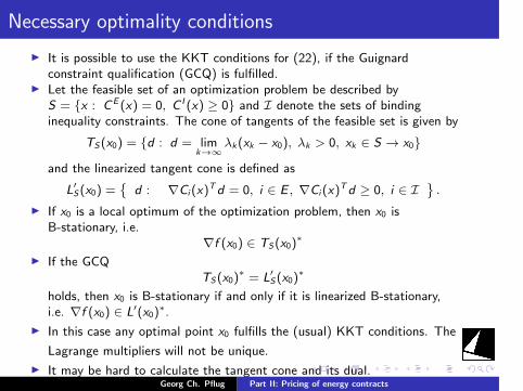
.
.
.
.
.
.
.
.
.
.
.
.
.
.
.
.
.
.
.
.
.
.
.
.
.
.
.
.
.
.
.
.
.
.
.
.
.
.
.
.
Necessary optimality conditions
I It is possible to use the KKT conditions for (22), if the Guignardconstraint qualification (GCQ) is fulfilled.
I Let the feasible set of an optimization problem be described byS = x : CE (x) = 0, C I (x) ≥ 0 and I denote the sets of bindinginequality constraints. The cone of tangents of the feasible set is given by
TS(x0) = d : d = limk→∞
λk(xk − x0), λk > 0, xk ∈ S → x0
and the linearized tangent cone is defined as
L′S(x0) =
d : ∇Ci (x)
Td = 0, i ∈ E , ∇Ci (x)Td ≥ 0, i ∈ I
.
I If x0 is a local optimum of the optimization problem, then x0 isB-stationary, i.e.
∇f (x0) ∈ TS(x0)∗
I If the GCQTS(x0)
∗ = L′S(x0)
∗
holds, then x0 is B-stationary if and only if it is linearized B-stationary,i.e. ∇f (x0) ∈ L′(x0)
∗.
I In this case any optimal point x0 fulfills the (usual) KKT conditions. The
Lagrange multipliers will not be unique.
I It may be hard to calculate the tangent cone and its dual.Georg Ch. Pflug Part II: Pricing of energy contracts
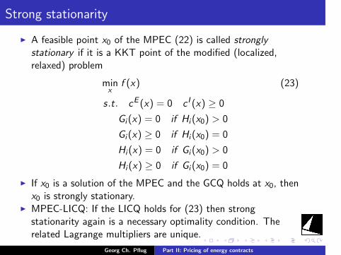
.
.
.
.
.
.
.
.
.
.
.
.
.
.
.
.
.
.
.
.
.
.
.
.
.
.
.
.
.
.
.
.
.
.
.
.
.
.
.
.
Strong stationarity
I A feasible point x0 of the MPEC (22) is called stronglystationary if it is a KKT point of the modified (localized,relaxed) problem
minx
f (x) (23)
s.t. cE (x) = 0 c I (x) ≥ 0
Gi (x) = 0 if Hi (x0) > 0
Gi (x) ≥ 0 if Hi (x0) = 0
Hi (x) = 0 if Gi (x0) > 0
Hi (x) ≥ 0 if Gi (x0) = 0
I If x0 is a solution of the MPEC and the GCQ holds at x0, thenx0 is strongly stationary.
I MPEC-LICQ: If the LICQ holds for (23) then strongstationarity again is a necessary optimality condition. Therelated Lagrange multipliers are unique.
Georg Ch. Pflug Part II: Pricing of energy contracts
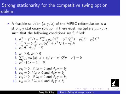
.
.
.
.
.
.
.
.
.
.
.
.
.
.
.
.
.
.
.
.
.
.
.
.
.
.
.
.
.
.
.
.
.
.
.
.
.
.
.
.
Strong stationarity for the competitive swing optionproblem
I A feasible solution (x , y , λ) of the MPEC reformulation is astrongly stationary solution if there exist multipliers µ, ν1, ν2such that the following conditions are fulfilled:
1. d⊤ + y⊤D =∑n
i=1 µ1i (qi⊤ + y⊤Q i⊤) + µ⊤
2 E − µ⊤3 C
⊤
2. x⊤D =∑nr
i=1 µ1i (qi⊤ + x⊤Q i )− ν⊤2 A
3. µ⊤3 A
⊤ + ν⊤1 = 0
4. µ1 ≥ 0, µ2 ≥ 05.
∑ni=1 µ1i
(qi⊤x x + qi⊤y y + x⊤Q iy − r i
)= 0
6. µ⊤2 · (Ex − ℓ) = 0
7. ν1j ≥ 0, if λj = 0 and Aj·y = bj8. ν1j = 0 if λj > 0 and Aj·y = bj9. ν2j ≥ 0, if λj = 0 and Aj·y = bj10. ν2j = 0 if λj = 0 and Aj·y < bj
Georg Ch. Pflug Part II: Pricing of energy contracts
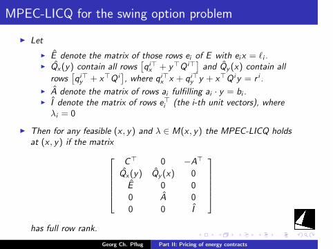
.
.
.
.
.
.
.
.
.
.
.
.
.
.
.
.
.
.
.
.
.
.
.
.
.
.
.
.
.
.
.
.
.
.
.
.
.
.
.
.
MPEC-LICQ for the swing option problem
I Let
I E denote the matrix of those rows ei of E with eix = ℓi .I Qx(y) contain all rows
[qi⊤x + y⊤Q i⊤] and Qy (x) contain all
rows[qi⊤y + x⊤Q i
], where qi⊤x x + qi⊤y y + x⊤Q iy = r i .
I A denote the matrix of rows ai fulfilling ai · y = bi .I I denote the matrix of rows e⊤i (the i-th unit vectors), where
λi = 0
I Then for any feasible (x , y) and λ ∈ M(x , y) the MPEC-LICQ holdsat (x , y) if the matrix
C⊤ 0 −A⊤
Qx(y) Qy (x) 0
E 0 0
0 A 0
0 0 I
has full row rank.
Georg Ch. Pflug Part II: Pricing of energy contracts
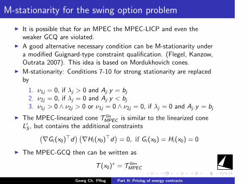
.
.
.
.
.
.
.
.
.
.
.
.
.
.
.
.
.
.
.
.
.
.
.
.
.
.
.
.
.
.
.
.
.
.
.
.
.
.
.
.
M-stationarity for the swing option problem
I It is possible that for an MPEC the MPEC-LICP and even theweaker GCQ are violated.
I A good alternative necessary condition can be M-stationarity undera modified Guignard-type constraint qualification. (Flegel, Kanzow,Outrata 2007). This idea is based on Mordukhovich cones.
I M-stationarity: Conditions 7-10 for strong stationarity are replacedby
1. ν1j = 0, if λj > 0 and Aj·y = bj2. ν2j = 0, if λj = 0 and Aj·y < bj3. ν1j > 0 ∧ ν2j > 0 or ν1j = 0 ∧ ν2j = 0, if λj = 0 and Aj·y = bj
I The MPEC-linearized cone T linMPEC is similar to the linearized cone
L′S , but contains the additional constraints(∇Gi (x0)
⊤d) (
∇Hi (x0)⊤d
)= 0, if Gi (x0) = Hi (x0) = 0
I The MPEC-GCQ then can be written as
T (x0)∗ = T lin∗
MPEC
Georg Ch. Pflug Part II: Pricing of energy contracts
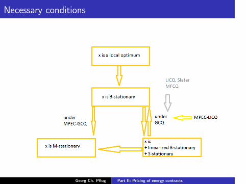
.
.
.
.
.
.
.
.
.
.
.
.
.
.
.
.
.
.
.
.
.
.
.
.
.
.
.
.
.
.
.
.
.
.
.
.
.
.
.
.
Necessary conditions
Georg Ch. Pflug Part II: Pricing of energy contracts
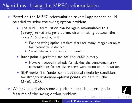
.
.
.
.
.
.
.
.
.
.
.
.
.
.
.
.
.
.
.
.
.
.
.
.
.
.
.
.
.
.
.
.
.
.
.
.
.
.
.
.
Algorithms: Using the MPEC-reformulation
I Based on the MPEC reformulation several approaches couldbe tried to solve the swing option problem
I The MPEC formulation can be again reformulated to a(binary) mixed integer problem, discriminating between thecases λi > 0 and λi = 0
I For the swing option problem there are many integer variablesfor reasonable instances
I Some bilinear constraints still remain
I Inner point algorithms are not applicable directly
I However, several methods for relaxing the complementarityconstraints or for penalizing them were proposed in literature.
I SQP works fine (under some additional regularity conditions)for strongly stationary optimal points, which fulfill theMPEC-LICQ.
I We developed also some algorithms that build on specialfeatures of the swing option problem.
Georg Ch. Pflug Part II: Pricing of energy contracts
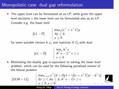
.
.
.
.
.
.
.
.
.
.
.
.
.
.
.
.
.
.
.
.
.
.
.
.
.
.
.
.
.
.
.
.
.
.
.
.
.
.
.
.
Monopolistic case: dual gap reformulation
I The upper level can be formulated as an LP, while given the upper
level decisions x the lower level can be formulated also as an LP.
Consider e.g. the lower level
[LL− P]
∣∣∣∣∣∣maxy (c
⊤ + x⊤C )yAy ≤ by ≥ 0
for some suitable vectors b, c1 and matrices A,C2.with dual
[LL− D]
∣∣∣∣∣∣minv b
⊤vA⊤v − C⊤x ≥ cv ≥ 0
I Minimizing the duality gap is equivalent to solving the lower levelproblem, which can be used for the following penalized version ofthe bilevel problem.
[ULM + LL]
∣∣∣∣∣∣maxx,v ;y x
⊤(d + Dy) + γ[(c + x⊤C )y − b⊤v ]Ex ≥ ℓ,Ay ≤ b,A⊤v − Cx ≥ cy ≥ 0, v ≥ 0.
(24)Georg Ch. Pflug Part II: Pricing of energy contracts
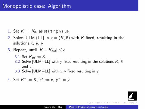
.
.
.
.
.
.
.
.
.
.
.
.
.
.
.
.
.
.
.
.
.
.
.
.
.
.
.
.
.
.
.
.
.
.
.
.
.
.
.
.
Monopolistic case: Algorithm
1. Set K := K0, as starting value
2. Solve [ULM+LL] in x = (K , x) with K fixed, resulting in thesolutions x , v , y
3. Repeat, until |K − Kold | ≤ ϵ
3.1 Set Kold := K3.2 Solve [ULM+LL] with y fixed resulting in the solutions K , x
and v3.3 Solve [ULM+LL] with x , v fixed resulting in y
4. Set K ∗ := K , x∗ := x , y∗ := y
Georg Ch. Pflug Part II: Pricing of energy contracts
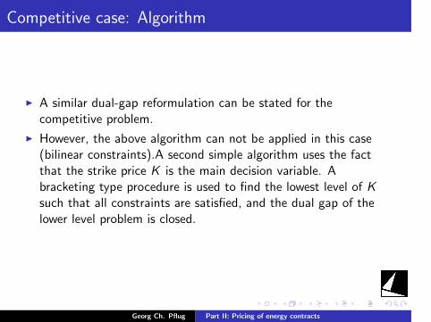
.
.
.
.
.
.
.
.
.
.
.
.
.
.
.
.
.
.
.
.
.
.
.
.
.
.
.
.
.
.
.
.
.
.
.
.
.
.
.
.
Competitive case: Algorithm
I A similar dual-gap reformulation can be stated for thecompetitive problem.
I However, the above algorithm can not be applied in this case(bilinear constraints).A second simple algorithm uses the factthat the strike price K is the main decision variable. Abracketing type procedure is used to find the lowest level of Ksuch that all constraints are satisfied, and the dual gap of thelower level problem is closed.
Georg Ch. Pflug Part II: Pricing of energy contracts
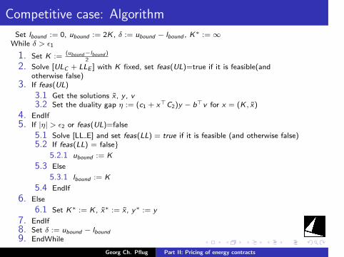
.
.
.
.
.
.
.
.
.
.
.
.
.
.
.
.
.
.
.
.
.
.
.
.
.
.
.
.
.
.
.
.
.
.
.
.
.
.
.
.
Competitive case: Algorithm
Set lbound := 0, ubound := 2K , δ := ubound − lbound , K∗ := ∞
While δ > ϵ1
1. Set K :=(ubound−lbound )
2
2. Solve [ULC + LLE ] with K fixed, set feas(UL)=true if it is feasible(andotherwise false)
3. If feas(UL)
3.1 Get the solutions x , y , v3.2 Set the duality gap η := (c1 + x⊤C2)y − b⊤v for x = (K , x)
4. EndIf5. If |η| > ϵ2 or feas(UL)=false
5.1 Solve [LL E] and set feas(LL) = true if it is feasible (and otherwise false)5.2 If feas(LL) = false
5.2.1 ubound := K
5.3 Else
5.3.1 lbound := K
5.4 EndIf
6. Else
6.1 Set K∗ := K , x∗ := x , y∗ := y
7. EndIf8. Set δ := ubound − lbound9. EndWhile
Georg Ch. Pflug Part II: Pricing of energy contracts
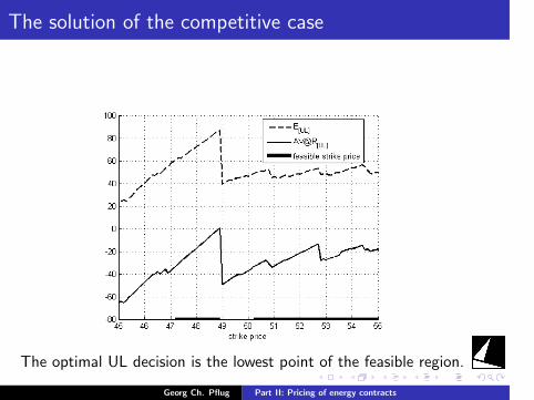
.
.
.
.
.
.
.
.
.
.
.
.
.
.
.
.
.
.
.
.
.
.
.
.
.
.
.
.
.
.
.
.
.
.
.
.
.
.
.
.
The solution of the competitive case
The optimal UL decision is the lowest point of the feasible region.
Georg Ch. Pflug Part II: Pricing of energy contracts
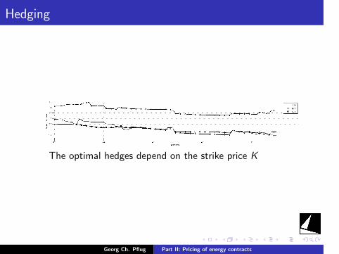
.
.
.
.
.
.
.
.
.
.
.
.
.
.
.
.
.
.
.
.
.
.
.
.
.
.
.
.
.
.
.
.
.
.
.
.
.
.
.
.
Hedging
The optimal hedges depend on the strike price K
Georg Ch. Pflug Part II: Pricing of energy contracts
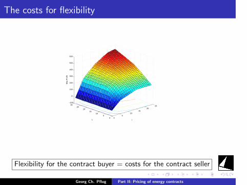
.
.
.
.
.
.
.
.
.
.
.
.
.
.
.
.
.
.
.
.
.
.
.
.
.
.
.
.
.
.
.
.
.
.
.
.
.
.
.
.
The costs for flexibility
05
1015
2025
05
1015
2025
30−100
0
100
200
300
400
500
600
lL
Max
Pro
fit
Flexibility for the contract buyer = costs for the contract seller
Georg Ch. Pflug Part II: Pricing of energy contracts
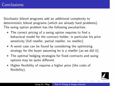
.
.
.
.
.
.
.
.
.
.
.
.
.
.
.
.
.
.
.
.
.
.
.
.
.
.
.
.
.
.
.
.
.
.
.
.
.
.
.
.
Conclusions
Stochastic bilevel programs add an additional complexity todeterministic bilevel programs (which are already hard problems).The swing option problem has the following peculiarities:
I The correct pricing of a swing option requires to find abehavioral model for the contract holder, in particular his pricesensitivity (full reseller, partial reseller, no reseller).
I A worst case can be found by considering the optimizingstrategy for the buyer assuming he is a reseller (as we did it).
I The optimal hedging strategies for fixed contracts and swingoptions may be quite different.
I Higher flexibility of requires a higher price (the costs offlexibility).
Georg Ch. Pflug Part II: Pricing of energy contracts
.
.
.
.
.
.
.
.
.
.
.
.
.
.
.
.
.
.
.
.
.
.
.
.
.
.
.
.
.
.
.
.
.
.
.
.
.
.
.
.
Part III: Optimal hydro management and theambiguity problem
Georg Ch. Pflug
July 3, 2016
Georg Ch. Pflug Part III: Optimal hydro management and the ambiguity problem
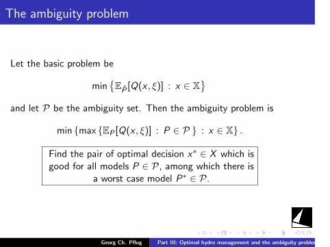
.
.
.
.
.
.
.
.
.
.
.
.
.
.
.
.
.
.
.
.
.
.
.
.
.
.
.
.
.
.
.
.
.
.
.
.
.
.
.
.
The ambiguity problem
Let the basic problem be
minEP [Q(x , ξ)] : x ∈ X
and let P be the ambiguity set. Then the ambiguity problem is
min max EP [Q(x , ξ)] : P ∈ P : x ∈ X .
Find the pair of optimal decision x∗ ∈ X which isgood for all models P ∈ P, among which there is
a worst case model P∗ ∈ P.
Georg Ch. Pflug Part III: Optimal hydro management and the ambiguity problem
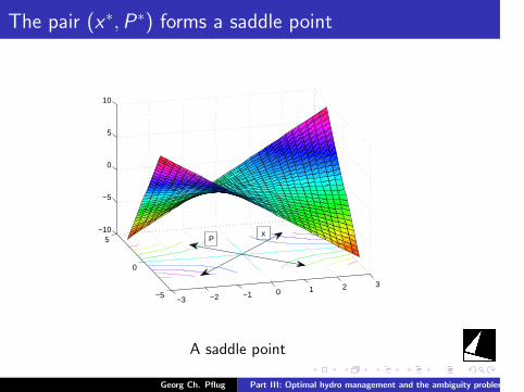
.
.
.
.
.
.
.
.
.
.
.
.
.
.
.
.
.
.
.
.
.
.
.
.
.
.
.
.
.
.
.
.
.
.
.
.
.
.
.
.
The pair (x∗,P∗) forms a saddle point
−3 −2 −1 0 1 2 3−5
0
5−10
−5
0
5
10
xP
A saddle point
Georg Ch. Pflug Part III: Optimal hydro management and the ambiguity problem
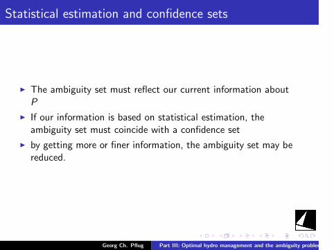
.
.
.
.
.
.
.
.
.
.
.
.
.
.
.
.
.
.
.
.
.
.
.
.
.
.
.
.
.
.
.
.
.
.
.
.
.
.
.
.
Statistical estimation and confidence sets
I The ambiguity set must reflect our current information aboutP
I If our information is based on statistical estimation, theambiguity set must coincide with a confidence set
I by getting more or finer information, the ambiguity set may bereduced.
Georg Ch. Pflug Part III: Optimal hydro management and the ambiguity problem
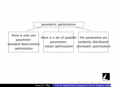
.
.
.
.
.
.
.
.
.
.
.
.
.
.
.
.
.
.
.
.
.
.
.
.
.
.
.
.
.
.
.
.
.
.
.
.
.
.
.
.
parametric optimization
there is only oneparameter:
standard deterministicoptimization
there is a set of possibleparameters:
robust optimization
the parameters arerandomly distributed:stochastic optimization
XXXXX
Georg Ch. Pflug Part III: Optimal hydro management and the ambiguity problem
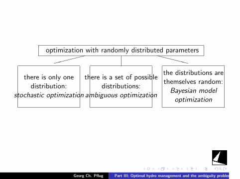
.
.
.
.
.
.
.
.
.
.
.
.
.
.
.
.
.
.
.
.
.
.
.
.
.
.
.
.
.
.
.
.
.
.
.
.
.
.
.
.
optimization with randomly distributed parameters
there is only onedistribution:
stochastic optimization
there is a set of possibledistributions:
ambiguous optimization
the distributions arethemselves random:Bayesian modeloptimization
XXXXX
Georg Ch. Pflug Part III: Optimal hydro management and the ambiguity problem
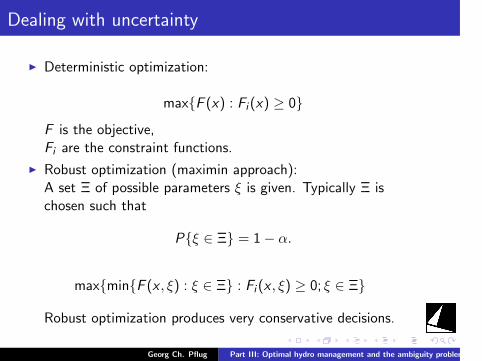
.
.
.
.
.
.
.
.
.
.
.
.
.
.
.
.
.
.
.
.
.
.
.
.
.
.
.
.
.
.
.
.
.
.
.
.
.
.
.
.
Dealing with uncertainty
I Deterministic optimization:
maxF (x) : Fi (x) ≥ 0
F is the objective,Fi are the constraint functions.
I Robust optimization (maximin approach):A set Ξ of possible parameters ξ is given. Typically Ξ ischosen such that
Pξ ∈ Ξ = 1− α.
maxminF (x , ξ) : ξ ∈ Ξ : Fi (x , ξ) ≥ 0; ξ ∈ Ξ
Robust optimization produces very conservative decisions.
Georg Ch. Pflug Part III: Optimal hydro management and the ambiguity problem
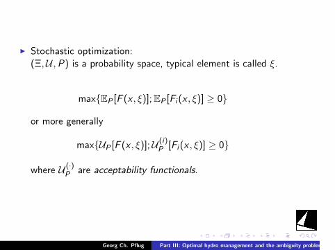
.
.
.
.
.
.
.
.
.
.
.
.
.
.
.
.
.
.
.
.
.
.
.
.
.
.
.
.
.
.
.
.
.
.
.
.
.
.
.
.
I Stochastic optimization:(Ξ,U ,P) is a probability space, typical element is called ξ.
maxEP [F (x , ξ)];EP [Fi (x , ξ)] ≥ 0
or more generally
maxUP [F (x , ξ)];U(i)P [Fi (x , ξ)] ≥ 0
where U (·)P are acceptability functionals.
Georg Ch. Pflug Part III: Optimal hydro management and the ambiguity problem
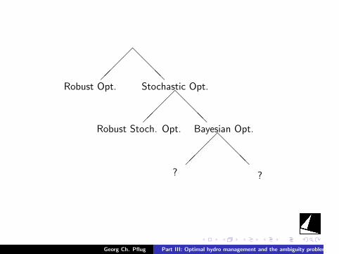
.
.
.
.
.
.
.
.
.
.
.
.
.
.
.
.
.
.
.
.
.
.
.
.
.
.
.
.
.
.
.
.
.
.
.
.
.
.
.
.
@@
@@Robust Opt. Stochastic Opt.
@@@@
Robust Stoch. Opt. Bayesian Opt.
@@
@@? ?
Georg Ch. Pflug Part III: Optimal hydro management and the ambiguity problem
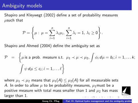
.
.
.
.
.
.
.
.
.
.
.
.
.
.
.
.
.
.
.
.
.
.
.
.
.
.
.
.
.
.
.
.
.
.
.
.
.
.
.
.
Ambiguity models
Shapiro and Kleywegt (2002) define a set of probability measuresµsuch that
P =
µ : µ =
n∑i=1
λiµi ,n∑
i=1
λi = 1, λi ≥ 0
.
Shapiro and Ahmed (2004) define the ambiguity set as
P =
µ is a prob. measure s.t. µ1 ≺ µ ≺ µ2,
∫ϕi dµ = bi ; i = 1, . . . k;∫
ψ dµ ≤ ci ; i = 1, . . . ℓ
where µ1 ≺ µ2 means that µ1(A) ≤ µ2(A) for all measurable setsA. In order to allow µ to be probability measures, µ1must be apositive measure with total mass smaller than 1 and µ2 has masslarger than 1.
Georg Ch. Pflug Part III: Optimal hydro management and the ambiguity problem
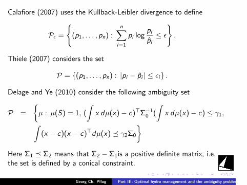
.
.
.
.
.
.
.
.
.
.
.
.
.
.
.
.
.
.
.
.
.
.
.
.
.
.
.
.
.
.
.
.
.
.
.
.
.
.
.
.
Calafiore (2007) uses the Kullback-Leibler divergence to define
Pϵ =
(p1, . . . , pn) :
n∑i=1
pi logpipi
≤ ϵ
.
Thiele (2007) considers the set
P = (p1, . . . , pn) : |pi − pi | ≤ ϵi .
Delage and Ye (2010) consider the following ambiguity set
P =
µ : µ(S) = 1, (
∫x dµ(x)− c)⊤Σ−1
0 (
∫x dµ(x)− c) ≤ γ1,∫
(x − c)(x − c)⊤dµ(x) ≼ γ2Σ0
Here Σ1 ≼ Σ2 means that Σ2 − Σ1is a positive definite matrix, i.e.the set is defined by a conical constraint.
Georg Ch. Pflug Part III: Optimal hydro management and the ambiguity problem
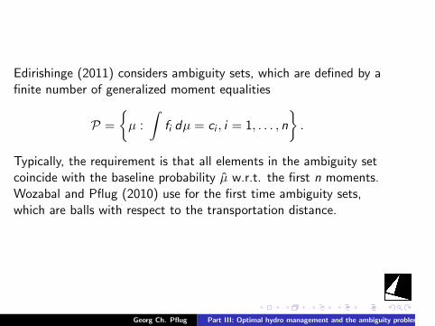
.
.
.
.
.
.
.
.
.
.
.
.
.
.
.
.
.
.
.
.
.
.
.
.
.
.
.
.
.
.
.
.
.
.
.
.
.
.
.
.
Edirishinge (2011) considers ambiguity sets, which are defined by afinite number of generalized moment equalities
P =
µ :
∫fi dµ = ci , i = 1, . . . , n
.
Typically, the requirement is that all elements in the ambiguity setcoincide with the baseline probability µ w.r.t. the first n moments.Wozabal and Pflug (2010) use for the first time ambiguity sets,which are balls with respect to the transportation distance.
Georg Ch. Pflug Part III: Optimal hydro management and the ambiguity problem
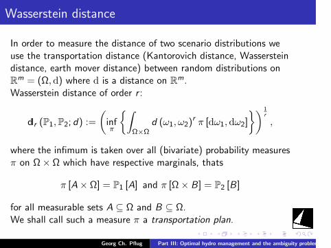
.
.
.
.
.
.
.
.
.
.
.
.
.
.
.
.
.
.
.
.
.
.
.
.
.
.
.
.
.
.
.
.
.
.
.
.
.
.
.
.
Wasserstein distance
In order to measure the distance of two scenario distributions weuse the transportation distance (Kantorovich distance, Wassersteindistance, earth mover distance) between random distributions onRm = (Ω, d) where d is a distance on Rm.Wasserstein distance of order r :
dlr (P1,P2; d) :=
(infπ
∫Ω×Ω
d (ω1, ω2)r π [dω1, dω2]
) 1r
,
where the infimum is taken over all (bivariate) probability measuresπ on Ω× Ω which have respective marginals, thats
π [A× Ω] = P1 [A] and π [Ω× B] = P2 [B]
for all measurable sets A ⊆ Ω and B ⊆ Ω.We shall call such a measure π a transportation plan.
Georg Ch. Pflug Part III: Optimal hydro management and the ambiguity problem
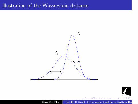
.
.
.
.
.
.
.
.
.
.
.
.
.
.
.
.
.
.
.
.
.
.
.
.
.
.
.
.
.
.
.
.
.
.
.
.
.
.
.
.
Illustration of the Wasserstein distance
Georg Ch. Pflug Part III: Optimal hydro management and the ambiguity problem
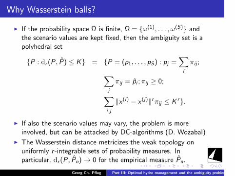
.
.
.
.
.
.
.
.
.
.
.
.
.
.
.
.
.
.
.
.
.
.
.
.
.
.
.
.
.
.
.
.
.
.
.
.
.
.
.
.
Why Wasserstein balls?
I If the probability space Ω is finite, Ω = ω(1), . . . , ω(S) andthe scenario values are kept fixed, then the ambiguity set is apolyhedral set
P : dr (P , P) ≤ K = P = (p1, . . . , pS) : pj =∑i
πij ;∑j
πij = pi ;πij ≥ 0;
∑i ,j
∥x (i) − x (j)∥rπij ≤ K r.
I If also the scenario values may vary, the problem is moreinvolved, but can be attacked by DC-algorithms (D. Wozabal)
I The Wasserstein distance metricizes the weak topology onuniformly r -integrable sets of probability measures. Inparticular, dr (P , Pn) → 0 for the empirical measure Pn.
Georg Ch. Pflug Part III: Optimal hydro management and the ambiguity problem
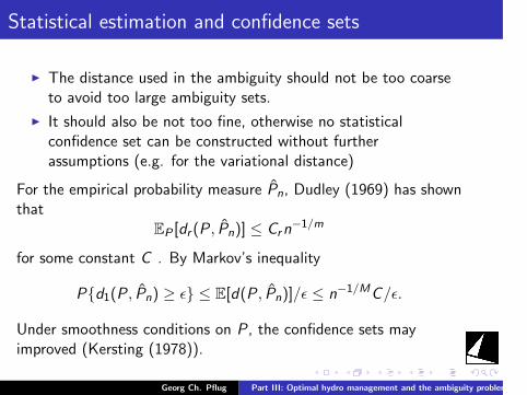
.
.
.
.
.
.
.
.
.
.
.
.
.
.
.
.
.
.
.
.
.
.
.
.
.
.
.
.
.
.
.
.
.
.
.
.
.
.
.
.
Statistical estimation and confidence sets
I The distance used in the ambiguity should not be too coarseto avoid too large ambiguity sets.
I It should also be not too fine, otherwise no statisticalconfidence set can be constructed without furtherassumptions (e.g. for the variational distance)
For the empirical probability measure Pn, Dudley (1969) has shownthat
EP [dr (P, Pn)] ≤ Crn−1/m
for some constant C . By Markov’s inequality
Pd1(P, Pn) ≥ ϵ ≤ E[d(P, Pn)]/ϵ ≤ n−1/MC/ϵ.
Under smoothness conditions on P, the confidence sets mayimproved (Kersting (1978)).
Georg Ch. Pflug Part III: Optimal hydro management and the ambiguity problem
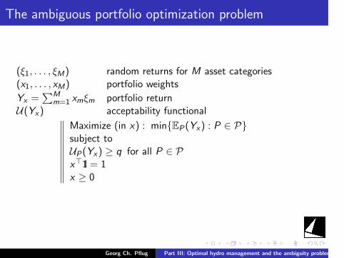
.
.
.
.
.
.
.
.
.
.
.
.
.
.
.
.
.
.
.
.
.
.
.
.
.
.
.
.
.
.
.
.
.
.
.
.
.
.
.
.
The ambiguous portfolio optimization problem
(ξ1, . . . , ξM) random returns for M asset categories(x1, . . . , xM) portfolio weights
Yx =∑M
m=1 xmξm portfolio returnU(Yx) acceptability functional∥∥∥∥∥∥∥∥∥∥
Maximize (in x) : minEP(Yx) : P ∈ Psubject toUP(Yx) ≥ q for all P ∈ Px⊤1l = 1x ≥ 0
Georg Ch. Pflug Part III: Optimal hydro management and the ambiguity problem
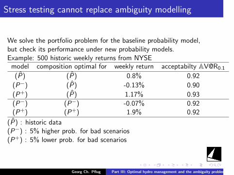
.
.
.
.
.
.
.
.
.
.
.
.
.
.
.
.
.
.
.
.
.
.
.
.
.
.
.
.
.
.
.
.
.
.
.
.
.
.
.
.
Stress testing cannot replace ambiguity modelling
We solve the portfolio problem for the baseline probability model,but check its performance under new probability models.Example: 500 historic weekly returns from NYSEmodel composition optimal for weekly return acceptabilty [email protected]
(P) (P) 0.8% 0.92
(P−) (P) -0.13% 0.90
(P+) (P) 1.17% 0.93
(P−) (P−) -0.07% 0.92(P+) (P+) 1.9% 0.92
(P) : historic data(P−) : 5% higher prob. for bad scenarios(P+) : 5% lower prob. for bad scenarios
Georg Ch. Pflug Part III: Optimal hydro management and the ambiguity problem
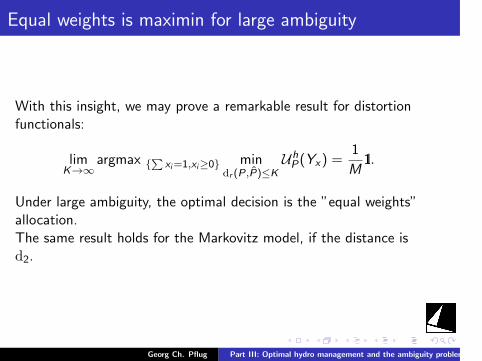
.
.
.
.
.
.
.
.
.
.
.
.
.
.
.
.
.
.
.
.
.
.
.
.
.
.
.
.
.
.
.
.
.
.
.
.
.
.
.
.
Equal weights is maximin for large ambiguity
With this insight, we may prove a remarkable result for distortionfunctionals:
limK→∞
argmax ∑
xi=1,xi≥0 mindr (P,P)≤K
UhP(Yx) =
1
M1l.
Under large ambiguity, the optimal decision is the ”equal weights”allocation.The same result holds for the Markovitz model, if the distance isd2.
Georg Ch. Pflug Part III: Optimal hydro management and the ambiguity problem
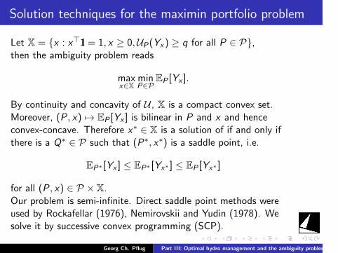
.
.
.
.
.
.
.
.
.
.
.
.
.
.
.
.
.
.
.
.
.
.
.
.
.
.
.
.
.
.
.
.
.
.
.
.
.
.
.
.
Solution techniques for the maximin portfolio problem
Let X = x : x⊤1l = 1, x ≥ 0,UP(Yx) ≥ q for all P ∈ P,then the ambiguity problem reads
maxx∈X
minP∈P
EP [Yx ].
By continuity and concavity of U , X is a compact convex set.Moreover, (P , x) 7→ EP [Yx ] is bilinear in P and x and henceconvex-concave. Therefore x∗ ∈ X is a solution of if and only ifthere is a Q∗ ∈ P such that (P∗, x∗) is a saddle point, i.e.
EP∗ [Yx ] ≤ EP∗ [Yx∗ ] ≤ EP [Yx∗ ]
for all (P, x) ∈ P × X.Our problem is semi-infinite. Direct saddle point methods wereused by Rockafellar (1976), Nemirovskii and Yudin (1978). Wesolve it by successive convex programming (SCP).
Georg Ch. Pflug Part III: Optimal hydro management and the ambiguity problem
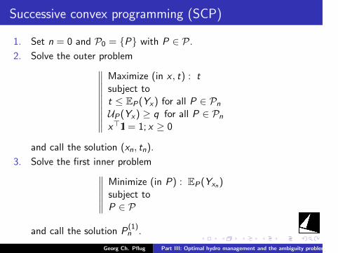
.
.
.
.
.
.
.
.
.
.
.
.
.
.
.
.
.
.
.
.
.
.
.
.
.
.
.
.
.
.
.
.
.
.
.
.
.
.
.
.
Successive convex programming (SCP)
1. Set n = 0 and P0 = P with P ∈ P.
2. Solve the outer problem∥∥∥∥∥∥∥∥∥∥Maximize (in x , t) : tsubject tot ≤ EP(Yx) for all P ∈ Pn
UP(Yx) ≥ q for all P ∈ Pn
x⊤1l = 1; x ≥ 0
and call the solution (xn, tn).
3. Solve the first inner problem∥∥∥∥∥∥Minimize (in P) : EP(Yxn)subject toP ∈ P
and call the solution P(1)n .
Georg Ch. Pflug Part III: Optimal hydro management and the ambiguity problem
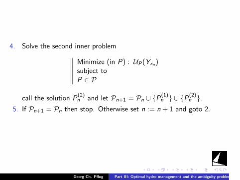
.
.
.
.
.
.
.
.
.
.
.
.
.
.
.
.
.
.
.
.
.
.
.
.
.
.
.
.
.
.
.
.
.
.
.
.
.
.
.
.
4. Solve the second inner problem∥∥∥∥∥∥Minimize (in P) : UP(Yxn)subject toP ∈ P
call the solution P(2)n and let Pn+1 = Pn ∪ P(1)
n ∪ P(2)n .
5. If Pn+1 = Pn then stop. Otherwise set n := n + 1 and goto 2.
Georg Ch. Pflug Part III: Optimal hydro management and the ambiguity problem
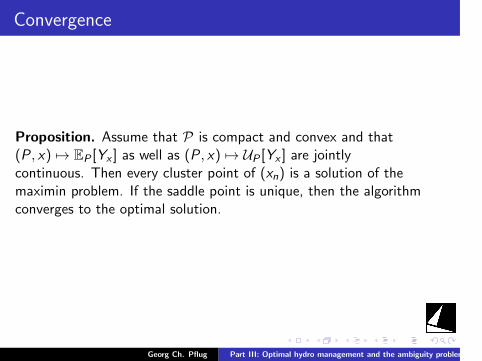
.
.
.
.
.
.
.
.
.
.
.
.
.
.
.
.
.
.
.
.
.
.
.
.
.
.
.
.
.
.
.
.
.
.
.
.
.
.
.
.
Convergence
Proposition. Assume that P is compact and convex and that(P , x) 7→ EP [Yx ] as well as (P, x) 7→ UP [Yx ] are jointlycontinuous. Then every cluster point of (xn) is a solution of themaximin problem. If the saddle point is unique, then the algorithmconverges to the optimal solution.
Georg Ch. Pflug Part III: Optimal hydro management and the ambiguity problem

.
.
.
.
.
.
.
.
.
.
.
.
.
.
.
.
.
.
.
.
.
.
.
.
.
.
.
.
.
.
.
.
.
.
.
.
.
.
.
.
P
Georg Ch. Pflug Part III: Optimal hydro management and the ambiguity problem
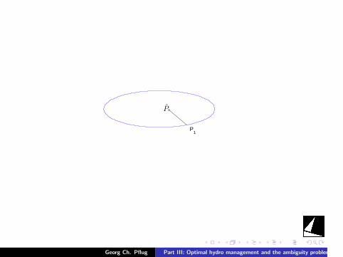
.
.
.
.
.
.
.
.
.
.
.
.
.
.
.
.
.
.
.
.
.
.
.
.
.
.
.
.
.
.
.
.
.
.
.
.
.
.
.
.
P
P1
Georg Ch. Pflug Part III: Optimal hydro management and the ambiguity problem
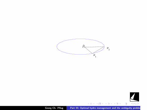
.
.
.
.
.
.
.
.
.
.
.
.
.
.
.
.
.
.
.
.
.
.
.
.
.
.
.
.
.
.
.
.
.
.
.
.
.
.
.
.
P
P1
P2
Georg Ch. Pflug Part III: Optimal hydro management and the ambiguity problem

.
.
.
.
.
.
.
.
.
.
.
.
.
.
.
.
.
.
.
.
.
.
.
.
.
.
.
.
.
.
.
.
.
.
.
.
.
.
.
.
P
P1
P2
P3
Georg Ch. Pflug Part III: Optimal hydro management and the ambiguity problem
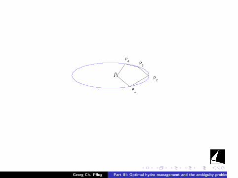
.
.
.
.
.
.
.
.
.
.
.
.
.
.
.
.
.
.
.
.
.
.
.
.
.
.
.
.
.
.
.
.
.
.
.
.
.
.
.
.
P
P1
P2
P4 P
3
Georg Ch. Pflug Part III: Optimal hydro management and the ambiguity problem
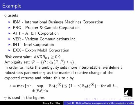
.
.
.
.
.
.
.
.
.
.
.
.
.
.
.
.
.
.
.
.
.
.
.
.
.
.
.
.
.
.
.
.
.
.
.
.
.
.
.
.
Example
6 assets
I IBM - International Business Machines CorporationI PRG - Procter & Gamble CorporationI ATT - AT&T CorporationI VER - Verizon Communications IncI INT - Intel CorporationI EXX - Exxon Mobil Corporation
Risk constraint: AV@R0,1 ≥ 0.9Ambiguity set: P = P : d1(P , P) ≤ ϵ.In order to make the ambiguity sets more interpretable, we define arobustness parameter γ as the maximal relative change of theexpected returns and relate this to ϵ by
ϵ = maxη : supd1(P,P)≤η
EP(ξ(i)) ≤ (1 + γ)EP(ξ
(i)) : for all i.
γ is used in the figures.Georg Ch. Pflug Part III: Optimal hydro management and the ambiguity problem
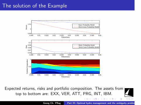
.
.
.
.
.
.
.
.
.
.
.
.
.
.
.
.
.
.
.
.
.
.
.
.
.
.
.
.
.
.
.
.
.
.
.
.
.
.
.
.
The solution of the Example
0.005 0.01 0.015 0.02 0.025 0.03 0.035 0.04 0.045 0.050.99
1
1.01
Robustness
Ret
urn
0.005 0.01 0.015 0.02 0.025 0.03 0.035 0.04 0.045 0.050.06
0.07
0.08
0.09
0.1
Robustness
Ris
k
0.005 0.01 0.015 0.02 0.025 0.03 0.035 0.04 0.045 0.050
0.5
1
Robustness
Por
tfolio
Com
posi
tion
Basic Probability ModelWorst Case Probability Model
Basic Probability ModelWorst Case Probability Model
Expected returns, risks and portfolio composition. The assets fromtop to bottom are: EXX, VER, ATT, PRG, INT, IBM.
Georg Ch. Pflug Part III: Optimal hydro management and the ambiguity problem
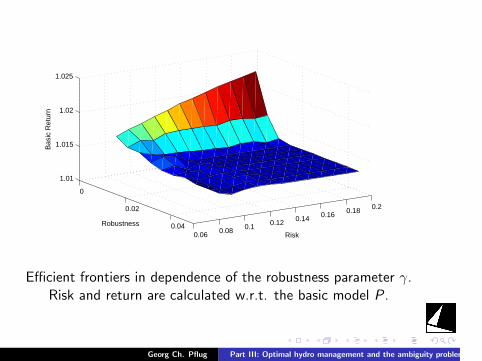
.
.
.
.
.
.
.
.
.
.
.
.
.
.
.
.
.
.
.
.
.
.
.
.
.
.
.
.
.
.
.
.
.
.
.
.
.
.
.
.
0
0.02
0.040.06 0.08 0.1 0.12 0.14 0.16 0.18 0.2
1.01
1.015
1.02
1.025
Risk
Robustness
Bas
ic R
etur
n
Efficient frontiers in dependence of the robustness parameter γ.Risk and return are calculated w.r.t. the basic model P .
Georg Ch. Pflug Part III: Optimal hydro management and the ambiguity problem
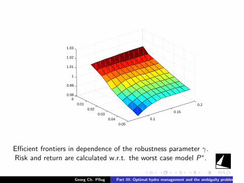
.
.
.
.
.
.
.
.
.
.
.
.
.
.
.
.
.
.
.
.
.
.
.
.
.
.
.
.
.
.
.
.
.
.
.
.
.
.
.
.
00.01
0.020.03
0.040.05
0.1
0.15
0.2
0.98
0.99
1
1.01
1.02
1.03
Efficient frontiers in dependence of the robustness parameter γ.Risk and return are calculated w.r.t. the worst case model P∗.
Georg Ch. Pflug Part III: Optimal hydro management and the ambiguity problem
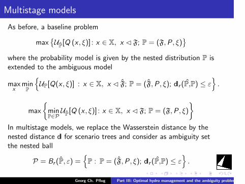
.
.
.
.
.
.
.
.
.
.
.
.
.
.
.
.
.
.
.
.
.
.
.
.
.
.
.
.
.
.
.
.
.
.
.
.
.
.
.
.
Multistage models
As before, a baseline problem
maxUP[Q (x , ξ)] : x ∈ X, x F; P = (F,P , ξ)
where the probability model is given by the nested distribution P isextended to the ambiguous model
maxx
minP
UP[Q(x , ξ)] : x ∈ X, x F; P = (F,P , ξ); dlr (P,P) ≤ ε
.
max
minP∈P
UP[Q (x , ξ)] : x ∈ X, x F; P = (F,P , ξ)
In multistage models, we replace the Wasserstein distance by thenested distance dl for scenario trees and consider as ambiguity setthe nested ball
P = Br (P, ε) =P : P = (F,P , ξ); dlr (P,P) ≤ ε
.
Georg Ch. Pflug Part III: Optimal hydro management and the ambiguity problem
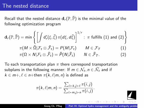
.
.
.
.
.
.
.
.
.
.
.
.
.
.
.
.
.
.
.
.
.
.
.
.
.
.
.
.
.
.
.
.
.
.
.
.
.
.
.
.
The nested distance
Recall that the nested distance dlr (P, P) is the minimal value of thefollowing optimization program
dlr (P, P) = min
[∫drr (ξ, ξ)π(dξ, d ξ)
]1/r: π fulfills (1) and (2)
π(M × Ω|Ft ⊗ Ft) = P(M|Ft) M ∈ FT (1)
π(Ω× N|Ft ⊗ Ft) = P(N|Ft) N ∈ FT . (2)
To each transportation plan π there correspond transportationsubplans in the following manner: If m ∈ Nt , n ∈ Nt and ifk ∈ m+, ℓ ∈ n+then π(k, ℓ|m, n) is defined as
π(k, ℓ|m, n) =∑
i≻k,j≻ℓ π(i , j)∑i≻m,j≻n π(i , j)
.
Georg Ch. Pflug Part III: Optimal hydro management and the ambiguity problem
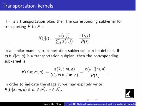
.
.
.
.
.
.
.
.
.
.
.
.
.
.
.
.
.
.
.
.
.
.
.
.
.
.
.
.
.
.
.
.
.
.
.
.
.
.
.
.
Transportation kernels
If π is a transportation plan, then the corresponding subkernel fortransporting P to P is
K (j |i) = π(i , j)∑j π(i , j)
=π(i , j)
P(i)
In a similar manner, transportation subkernels can be defined. Ifπ(k, ℓ|m, n) is a transportation subplan, then the correspondingsubkernel is
K (ℓ|k ;m, n) := π(k , ℓ|m, n)∑ℓ π(k, l |m, n)
=π(k , ℓ|m, n)
P(k).
In order to indicate the stage t, we may explitely writeKt(·|k,m, n) if m ∈ Nt , n ∈ Nt .
Georg Ch. Pflug Part III: Optimal hydro management and the ambiguity problem

.
.
.
.
.
.
.
.
.
.
.
.
.
.
.
.
.
.
.
.
.
.
.
.
.
.
.
.
.
.
.
.
.
.
.
.
.
.
.
.
Notice that the subkernels satisfy
Kt(ℓ | k ;m, n) ≥ 0,∑ℓ∈n+
Kt(ℓ | i ;m, n) = 1
and can be interpreted as Markov transition operators.The transportation plan π satisfies the ”filtration constraints”, iff
K (j |i) = K1 · · · KT−1(j |i)= K1(j1) | i1; 1, 1) · · · · · ·K (jT−1 | iT−1; iT−2, jT−2)×
×K (j | i ; iT−1, jT−1).
Georg Ch. Pflug Part III: Optimal hydro management and the ambiguity problem
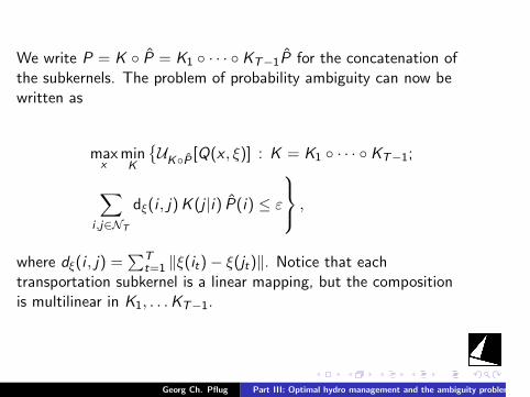
.
.
.
.
.
.
.
.
.
.
.
.
.
.
.
.
.
.
.
.
.
.
.
.
.
.
.
.
.
.
.
.
.
.
.
.
.
.
.
.
We write P = K P = K1 · · · KT−1P for the concatenation ofthe subkernels. The problem of probability ambiguity can now bewritten as
maxx
minK
UKP [Q(x , ξ)] : K = K1 · · · KT−1;
∑i ,j∈NT
dξ(i , j)K (j |i) P(i) ≤ ε
,
where dξ(i , j) =∑T
t=1 ∥ξ(it)− ξ(jt)∥. Notice that eachtransportation subkernel is a linear mapping, but the compositionis multilinear in K1, . . .KT−1.
Georg Ch. Pflug Part III: Optimal hydro management and the ambiguity problem
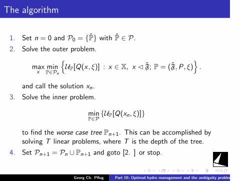
.
.
.
.
.
.
.
.
.
.
.
.
.
.
.
.
.
.
.
.
.
.
.
.
.
.
.
.
.
.
.
.
.
.
.
.
.
.
.
.
The algorithm
1. Set n = 0 and P0 = P with P ∈ P.
2. Solve the outer problem.
maxx
minP∈Pn
UP[Q(x , ξ)] : x ∈ X, x F; P = (F,P, ξ)
.
and call the solution xn.
3. Solve the inner problem.
minP∈P
UP[Q(xn, ξ)]
to find the worse case tree Pn+1. This can be accomplished bysolving T linear problems, where T is the depth of the tree.
4. Set Pn+1 = Pn ∪ Pn+1 and goto [2. ] or stop.
Georg Ch. Pflug Part III: Optimal hydro management and the ambiguity problem

.
.
.
.
.
.
.
.
.
.
.
.
.
.
.
.
.
.
.
.
.
.
.
.
.
.
.
.
.
.
.
.
.
.
.
.
.
.
.
.
Price of Ambiguity and Reward for Robustness
Let P be the baseline model and let x∗(P) be the optimal solutionof the baseline problem. Likewise, let P be the ambiguity set andlet x∗(P) be the solution of the minimax problem. Underconvex-concavity, the solution x∗(P) of the minimax problemtogether with the worst case model P∗ form a saddle point,meaning that the following inequality is valid for all feasible x andall P ∈ P
EP[Q(x∗(P), ξ)] ≤ EP∗ [Q(x∗(P), ξ)] ≤ EP∗ [Q(x , ξ)].
Let us call EP∗ [Q(x∗(P), ξ)] the minimax value.
Georg Ch. Pflug Part III: Optimal hydro management and the ambiguity problem
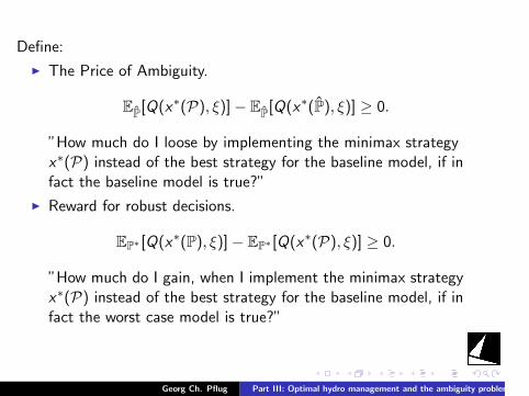
.
.
.
.
.
.
.
.
.
.
.
.
.
.
.
.
.
.
.
.
.
.
.
.
.
.
.
.
.
.
.
.
.
.
.
.
.
.
.
.
Define:
I The Price of Ambiguity.
EP[Q(x∗(P), ξ)]− EP[Q(x∗(P), ξ)] ≥ 0.
”How much do I loose by implementing the minimax strategyx∗(P) instead of the best strategy for the baseline model, if infact the baseline model is true?”
I Reward for robust decisions.
EP∗ [Q(x∗(P), ξ)]− EP∗ [Q(x∗(P), ξ)] ≥ 0.
”How much do I gain, when I implement the minimax strategyx∗(P) instead of the best strategy for the baseline model, if infact the worst case model is true?”
Georg Ch. Pflug Part III: Optimal hydro management and the ambiguity problem
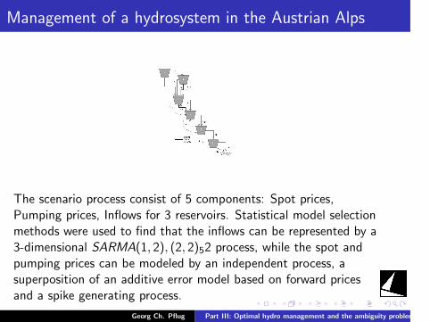
.
.
.
.
.
.
.
.
.
.
.
.
.
.
.
.
.
.
.
.
.
.
.
.
.
.
.
.
.
.
.
.
.
.
.
.
.
.
.
.
Management of a hydrosystem in the Austrian Alps
The scenario process consist of 5 components: Spot prices,Pumping prices, Inflows for 3 reservoirs. Statistical model selectionmethods were used to find that the inflows can be represented by a3-dimensional SARMA(1, 2), (2, 2)52 process, while the spot andpumping prices can be modeled by an independent process, asuperposition of an additive error model based on forward pricesand a spike generating process.
Georg Ch. Pflug Part III: Optimal hydro management and the ambiguity problem
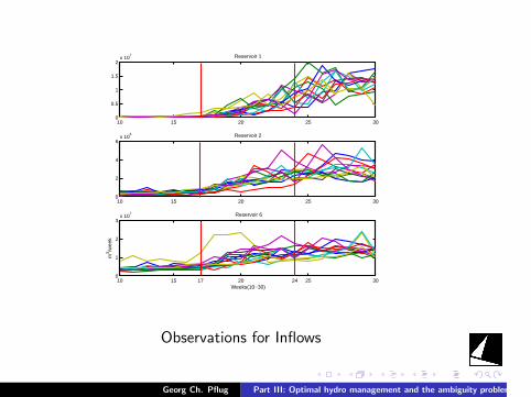
.
.
.
.
.
.
.
.
.
.
.
.
.
.
.
.
.
.
.
.
.
.
.
.
.
.
.
.
.
.
.
.
.
.
.
.
.
.
.
.
10 15 20 25 300
0.5
1
1.5
2x 10
7 Reservoir 1
10 15 20 25 300
2
4
6x 10
6 Reservoir 2
10 15 17 20 24 25 300
1
2
3x 10
7
Weeks(10−30)
m3 /w
eek
Reservoir 6
Observations for Inflows
Georg Ch. Pflug Part III: Optimal hydro management and the ambiguity problem
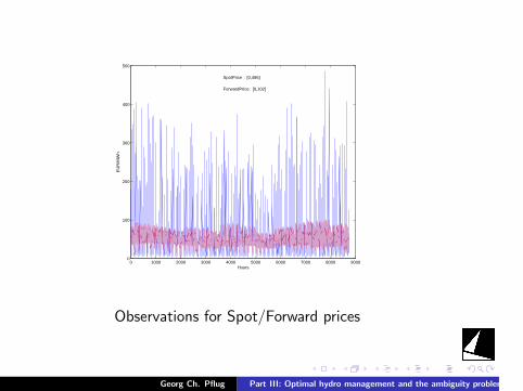
.
.
.
.
.
.
.
.
.
.
.
.
.
.
.
.
.
.
.
.
.
.
.
.
.
.
.
.
.
.
.
.
.
.
.
.
.
.
.
.
0 1000 2000 3000 4000 5000 6000 7000 8000 90000
100
200
300
400
500
SpotPrice : [0,486]
ForwardPrice: [0,102]
Hours
EU
R/M
Wh
Observations for Spot/Forward prices
Georg Ch. Pflug Part III: Optimal hydro management and the ambiguity problem
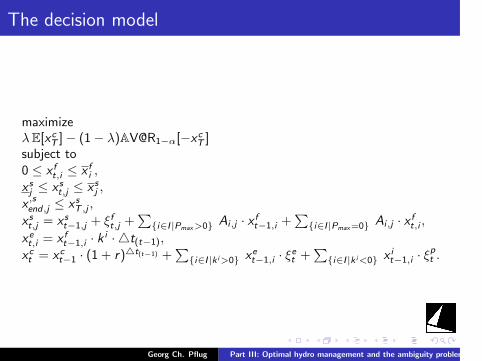
.
.
.
.
.
.
.
.
.
.
.
.
.
.
.
.
.
.
.
.
.
.
.
.
.
.
.
.
.
.
.
.
.
.
.
.
.
.
.
.
The decision model
maximizeλE[xcT ]− (1− λ)AV@R1−α[−xcT ]subject to0 ≤ x ft,i ≤ x fi ,x sj ≤ x st,j ≤ x sj ,x ,send,j ≤ x sT ,j ,
x st,j = x st−1,j + ξft,j +∑
i∈I |Pmax>0 Ai,j · x ft−1,i +∑
i∈I |Pmax=0 Ai,j · x ft,i ,xet,i = x ft−1,i · k i · t(t−1),
xct = xct−1 · (1 + r)t(t−1) +∑
i∈I |k i>0 xet−1,i · ξet +∑
i∈I |k i<0 x it−1,i · ξpt .
Georg Ch. Pflug Part III: Optimal hydro management and the ambiguity problem
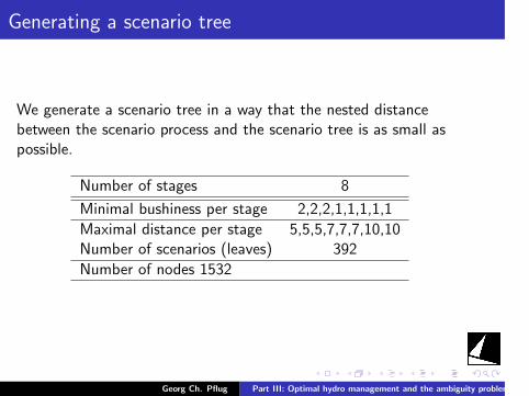
.
.
.
.
.
.
.
.
.
.
.
.
.
.
.
.
.
.
.
.
.
.
.
.
.
.
.
.
.
.
.
.
.
.
.
.
.
.
.
.
Generating a scenario tree
We generate a scenario tree in a way that the nested distancebetween the scenario process and the scenario tree is as small aspossible.
Number of stages 8
Minimal bushiness per stage 2,2,2,1,1,1,1,1
Maximal distance per stage 5,5,5,7,7,7,10,10Number of scenarios (leaves) 392
Number of nodes 1532
Georg Ch. Pflug Part III: Optimal hydro management and the ambiguity problem
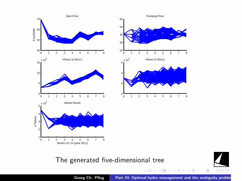
.
.
.
.
.
.
.
.
.
.
.
.
.
.
.
.
.
.
.
.
.
.
.
.
.
.
.
.
.
.
.
.
.
.
.
.
.
.
.
.
0 1 2 3 4 5 6 7 840
50
60
70
Eur
o/M
Wh
Spot Price
0 1 2 3 4 5 6 7 820
30
40
50
60Pumping Price
0 1 2 3 4 5 6 7 80
5
10
15x 10
5 Inflows to Resv1
0 1 2 3 4 5 6 7 82
3
4
5x 10
5 Inflows to Resv2
0 1 2 3 4 5 6 7 81
2
3
4
5x 10
6
Weeks 16−24 (year 2011)
m3 /W
eek
Inflows Resv6
The generated five-dimensional tree
Georg Ch. Pflug Part III: Optimal hydro management and the ambiguity problem
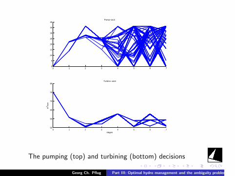
.
.
.
.
.
.
.
.
.
.
.
.
.
.
.
.
.
.
.
.
.
.
.
.
.
.
.
.
.
.
.
.
.
.
.
.
.
.
.
.
0 1 2 3 4 5 6 70
5
10
15
20
25
30
35
40Pump−arc4
0 1 2 3 4 5 6 755
60
65
70
75
80
stages
m3 /s
ec
Turbine−arc6
The pumping (top) and turbining (bottom) decisions
Georg Ch. Pflug Part III: Optimal hydro management and the ambiguity problem
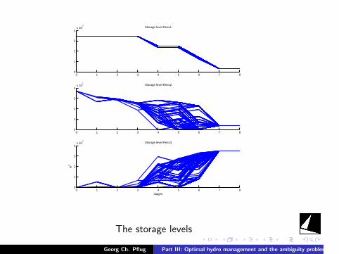
.
.
.
.
.
.
.
.
.
.
.
.
.
.
.
.
.
.
.
.
.
.
.
.
.
.
.
.
.
.
.
.
.
.
.
.
.
.
.
.
0 1 2 3 4 5 6 7 80
1
2
3
4x 10
7 Storage level Resv1
0 1 2 3 4 5 6 7 80
1
2
3
4x 10
7 Storage level Resv2
0 1 2 3 4 5 6 7 80
1
2
3
4x 10
7
stages
m3
Storage level Resv3
The storage levels
Georg Ch. Pflug Part III: Optimal hydro management and the ambiguity problem
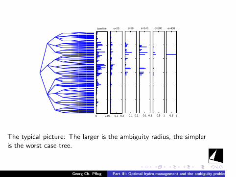
.
.
.
.
.
.
.
.
.
.
.
.
.
.
.
.
.
.
.
.
.
.
.
.
.
.
.
.
.
.
.
.
.
.
.
.
.
.
.
.
0 0.05
baseline
0.1 0.2
e=20
0.1 0.2
e=80
0.1 0.2
e=140
0.5 1
e=200
0.5 1
e=400
The typical picture: The larger is the ambiguity radius, the simpleris the worst case tree.
Georg Ch. Pflug Part III: Optimal hydro management and the ambiguity problem
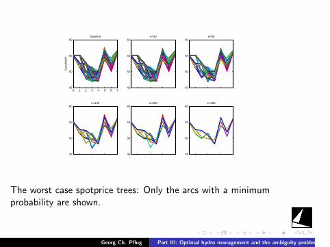
.
.
.
.
.
.
.
.
.
.
.
.
.
.
.
.
.
.
.
.
.
.
.
.
.
.
.
.
.
.
.
.
.
.
.
.
.
.
.
.
0 1 2 3 4 5 6 745
50
55
60
Eur
o/M
Wh
baseline
45
50
55
60e=20
45
50
55
60e=80
45
50
55
60e=140
45
50
55
60e=200
45
50
55
60e=400
The worst case spotprice trees: Only the arcs with a minimumprobability are shown.
Georg Ch. Pflug Part III: Optimal hydro management and the ambiguity problem
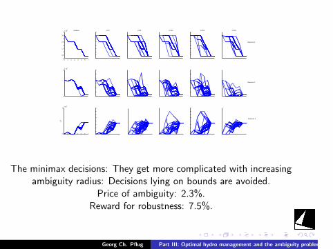
.
.
.
.
.
.
.
.
.
.
.
.
.
.
.
.
.
.
.
.
.
.
.
.
.
.
.
.
.
.
.
.
.
.
.
.
.
.
.
.
0 1 2 3 4 5 6 70
0.5
1
1.5
2
2.5
3
3.5
4x 10
7 baseline e=20 e=80 e=140 e=200 e=400
0
6x 10
7
0
8x 10
7
m3
Reservoir 1
Reservoir 2
Reservoir 3
The minimax decisions: They get more complicated with increasingambiguity radius: Decisions lying on bounds are avoided.
Price of ambiguity: 2.3%.Reward for robustness: 7.5%.
Georg Ch. Pflug Part III: Optimal hydro management and the ambiguity problem
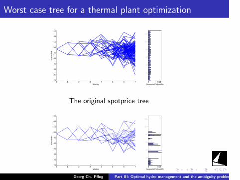
.
.
.
.
.
.
.
.
.
.
.
.
.
.
.
.
.
.
.
.
.
.
.
.
.
.
.
.
.
.
.
.
.
.
.
.
.
.
.
.
Worst case tree for a thermal plant optimization
0 1 2 3 4 5 6 720
25
30
35
40
45
50
55
60
65
Weeks
Eur
o/M
Wh
0 0.05
20
40
60
80
100
120
Scenario Probability
The original spotprice tree
0 1 2 3 4 5 6 720
25
30
35
40
45
50
55
60
65
Weeks
Eur
o/M
Wh
0 0.05
20
40
60
80
100
120
Scenario Probability
The worst case spotprice tree
Georg Ch. Pflug Part III: Optimal hydro management and the ambiguity problem
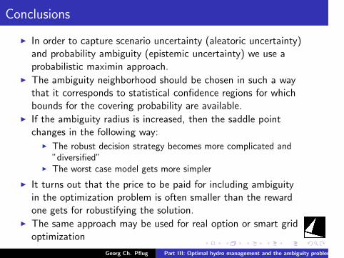
.
.
.
.
.
.
.
.
.
.
.
.
.
.
.
.
.
.
.
.
.
.
.
.
.
.
.
.
.
.
.
.
.
.
.
.
.
.
.
.
Conclusions
I In order to capture scenario uncertainty (aleatoric uncertainty)and probability ambiguity (epistemic uncertainty) we use aprobabilistic maximin approach.
I The ambiguity neighborhood should be chosen in such a waythat it corresponds to statistical confidence regions for whichbounds for the covering probability are available.
I If the ambiguity radius is increased, then the saddle pointchanges in the following way:
I The robust decision strategy becomes more complicated and”diversified”
I The worst case model gets more simpler
I It turns out that the price to be paid for including ambiguityin the optimization problem is often smaller than the rewardone gets for robustifying the solution.
I The same approach may be used for real option or smart gridoptimization
Georg Ch. Pflug Part III: Optimal hydro management and the ambiguity problem

Decision making under uncertainty
Georg Ch. Pflug
April 19, 2016
Georg Ch. Pflug Decision making under uncertainty

Our Springer book
Georg Ch. Pflug Decision making under uncertainty
Robust decisions
Wikipedia: Robust decision first used in the late 1990s. It is usedto identify decisions made with a process that includes formalconsideration of uncertainty. A robust decision is the best possiblechoice, one found by eliminating all the uncertainty possible withinavailable resources, and then choosing, with known and acceptablelevels of satisfaction and risk. (David G. Ullman)Stochastic optimization methods are optimization methods thatgenerate and use random variables. For stochastic problems, therandom variables appear in the formulation of the optimizationproblem itself, which involve random objective functions or randomconstraints, for example.
Georg Ch. Pflug Decision making under uncertainty
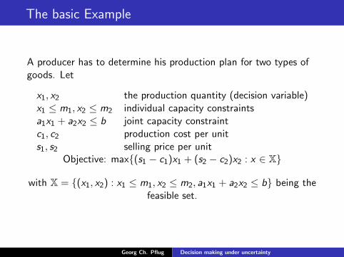
The basic Example
A producer has to determine his production plan for two types ofgoods. Let
x1, x2 the production quantity (decision variable)x1 ≤ m1, x2 ≤ m2 individual capacity constraintsa1x1 + a2x2 ≤ b joint capacity constraintc1, c2 production cost per units1, s2 selling price per unit
Objective: max(s1 − c1)x1 + (s2 − c2)x2 : x ∈ X
with X = (x1, x2) : x1 ≤ m1, x2 ≤ m2, a1x1 + a2x2 ≤ b being thefeasible set.
Georg Ch. Pflug Decision making under uncertainty
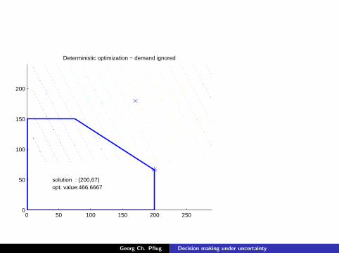
0 50 100 150 200 2500
50
100
150
200
Deterministic optimization − demand ignored
solution : (200,67)opt. value:466.6667
Georg Ch. Pflug Decision making under uncertainty
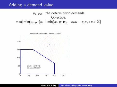
Adding a demand value
µ1, µ2 the deterministic demandsObjective:
maxmin(x1, µ1)s1 +min(x2, µ2)s2 − c1x1 − c2x2 : x ∈ X
0 50 100 150 200 2500
50
100
150
200
Deterministic optimization − demand included
solution : (170,87)opt. value:426.6667
Georg Ch. Pflug Decision making under uncertainty
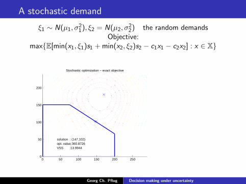
A stochastic demand
ξ1 ∼ N(µ1, σ21), ξ2 = N(µ2, σ
22) the random demands
Objective:maxE[min(x1, ξ1)s1 +min(x2, ξ2)s2 − c1x1 − c2x2] : x ∈ X
0 50 100 150 200 2500
50
100
150
200
Stochastic optimization − exact objective
solution : (147,102)opt. value:360.8726VSS :13.9944
Georg Ch. Pflug Decision making under uncertainty
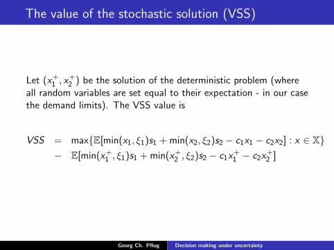
The value of the stochastic solution (VSS)
Let (x+1 , x+2 ) be the solution of the deterministic problem (whereall random variables are set equal to their expectation - in our casethe demand limits). The VSS value is
VSS = maxE[min(x1, ξ1)s1 +min(x2, ξ2)s2 − c1x1 − c2x2] : x ∈ X− E[min(x+1 , ξ1)s1 +min(x+2 , ξ2)s2 − c1x
+1 − c2x
+2 ]
Georg Ch. Pflug Decision making under uncertainty
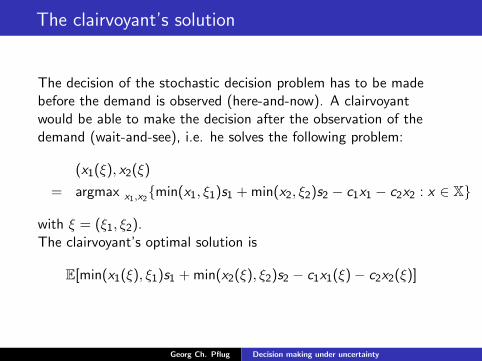
The clairvoyant’s solution
The decision of the stochastic decision problem has to be madebefore the demand is observed (here-and-now). A clairvoyantwould be able to make the decision after the observation of thedemand (wait-and-see), i.e. he solves the following problem:
(x1(ξ), x2(ξ)
= argmax x1,x2min(x1, ξ1)s1 +min(x2, ξ2)s2 − c1x1 − c2x2 : x ∈ X
with ξ = (ξ1, ξ2).The clairvoyant’s optimal solution is
E[min(x1(ξ), ξ1)s1 +min(x2(ξ), ξ2)s2 − c1x1(ξ)− c2x2(ξ)]
Georg Ch. Pflug Decision making under uncertainty
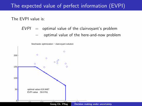
The expected value of perfect information (EVPI)
The EVPI value is:
EVPI = optimal value of the clairvoyant’s problem
− optimal value of the here-and-now problem
0 50 100 150 200 2500
50
100
150
200
Stochastic optimization − clairvoyant solution
optimal value:419.9487EVPI value :59.0761
Georg Ch. Pflug Decision making under uncertainty
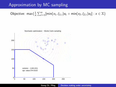
Approximation by MC sampling
Objective: max 1n
∑ni=1[min(x1, ξ1,i )s1 +min(x2, ξ2,i )s2] : x ∈ X
0 50 100 150 200 2500
50
100
150
200
Stochastic optimization − Monte Carlo sampling
solution : (148,101)opt. value:374.5315
Georg Ch. Pflug Decision making under uncertainty
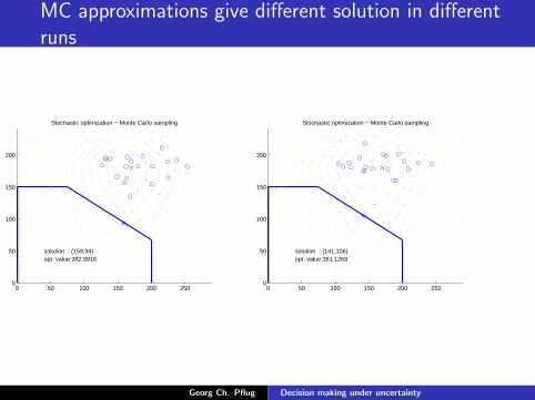
MC approximations give different solution in differentruns
0 50 100 150 200 2500
50
100
150
200
Stochastic optimization − Monte Carlo sampling
solution : (159,94)opt. value:382.9916
0 50 100 150 200 2500
50
100
150
200
Stochastic optimization − Monte Carlo sampling
solution : (141,106)opt. value:361.1269
Georg Ch. Pflug Decision making under uncertainty
Approximation by quantization
Instead of sampling, one may use optimally placed weighted points,which are chosen in order to minimize a distance between themand the probability distribution of the problem.To calculate optimal points is a nonlinear nonconvex optimizationproblem of its own. For the normal distributions, optimal pointshave been calculated by Gilles Pages and published on hisweb-pages (the Pages-pages).
Georg Ch. Pflug Decision making under uncertainty
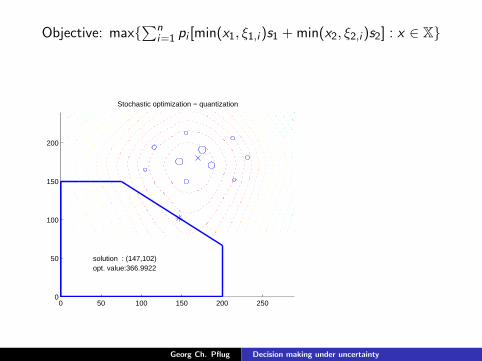
Objective: max∑n
i=1 pi [min(x1, ξ1,i )s1 +min(x2, ξ2,i )s2] : x ∈ X
0 50 100 150 200 2500
50
100
150
200
Stochastic optimization − quantization
solution : (147,102)opt. value:366.9922
Georg Ch. Pflug Decision making under uncertainty
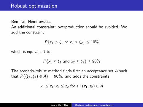
Robust optimization
Ben-Tal, Nemirovski,...An additional constraint: overproduction should be avoided. Weadd the constraint
Px1 > ξ1 or x2 > ξ2 ≤ 10%
which is equivalent to
Px1 ≤ ξ1 and x2 ≤ ξ2 ≥ 90%
The scenario-robust method finds first an acceptance set A suchthat P(ξ1, ξ2) ∈ A = 90%. and adds the constraints
x1 ≤ z1; x2 ≤ z2 for all (z1, z2) ∈ A
Georg Ch. Pflug Decision making under uncertainty
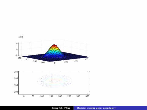
0 100 200 300100
150200
2500
1
2
x 10−4
0 50 100 150 200 250 300 350
100
150
200
250
Georg Ch. Pflug Decision making under uncertainty
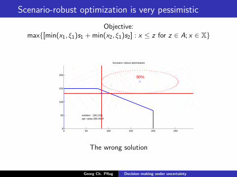
Scenario-robust optimization is very pessimistic
Objective:max[min(x1, ξ1)s1 +min(x2, ξ1)s2] : x ≤ z for z ∈ A; x ∈ X
0 50 100 150 200 2500
50
100
150
200
Scenario−robust optimization
solution : (84,132)opt. value:300.4034
90%
The wrong solution
Georg Ch. Pflug Decision making under uncertainty
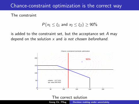
Chance-constraint optimization is the correct way
The constraint
Px1 ≤ ξ1 and x2 ≤ ξ2 ≥ 90%
is added to the constraint set, but the acceptance set A maydepend on the solution x and is not chosen beforehand.
0 50 100 150 200 2500
50
100
150
200
Chance−constrained stochastic optimization
solution : (117,122)opt. value:345.5416
90%
The correct solutionGeorg Ch. Pflug Decision making under uncertainty

Robust optimization-an additional example
Suppose that an investment can be made in 3 different assets andthat 5 equally probable scenarios for the returns are given. The5× 3 data matrix
1.10 0.96 0.961.08 1.06 1.051.02 1.06 1.050.98 1.01 1.001.00 1.00 0.90
ω1
ω2
ω3
ω4
ω5
ξ1 ξ2 ξ3
collects the 5 possible outcomes of the return variableξ = (ξ1,, ξ2, ξ3).
Georg Ch. Pflug Decision making under uncertainty
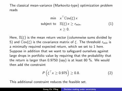
The classical mean-variance (Markovitz-type) optimization problemreads
min x⊤Cov(ξ) xsubject to E(ξ) x ≥ rmin, (1)
x ≥ 0.
Here, E(ξ) is the mean return vector (columnwise sums divided by5) and Cov(ξ) is the covariance matrix of ξ. The threshold rmin isa minimally required expected return, which we set to 1 here.Suppose in addition that we want to safeguard ourselves againstlarge drops in portfolio value by requiring that the probability thatthe return is larger than 0.9750 (say) is at least 80 %. We wouldthen add the constraint
P(ξ⊤x ≥ 0.975
)≥ 0.8. (2)
This additional constraint reduces the feasible set.
Georg Ch. Pflug Decision making under uncertainty
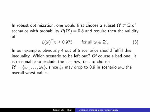
In robust optimization, one would first choose a subset Ω′ ⊂ Ω ofscenarios with probability P(Ω′) = 0.8 and require then the validityof
ξ(ω)⊤x ≥ 0.975 for all ω ∈ Ω′. (3)
In our example, obviously 4 out of 5 scenarios should fulfill thisinequality. Which scenario to be left out? Of course a bad one. Itis reasonable to exclude the last row, i.e., to chooseΩ′ = ω1, . . . , ω4, since ξ3 may drop to 0.9 in scenario ω5, theoverall worst value.
Georg Ch. Pflug Decision making under uncertainty
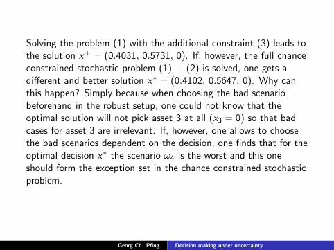
Solving the problem (1) with the additional constraint (3) leads tothe solution x+ = (0.4031, 0.5731, 0). If, however, the full chanceconstrained stochastic problem (1) + (2) is solved, one gets adifferent and better solution x∗ = (0.4102, 0.5647, 0). Why canthis happen? Simply because when choosing the bad scenariobeforehand in the robust setup, one could not know that theoptimal solution will not pick asset 3 at all (x3 = 0) so that badcases for asset 3 are irrelevant. If, however, one allows to choosethe bad scenarios dependent on the decision, one finds that for theoptimal decision x∗ the scenario ω4 is the worst and this oneshould form the exception set in the chance constrained stochasticproblem.
Georg Ch. Pflug Decision making under uncertainty
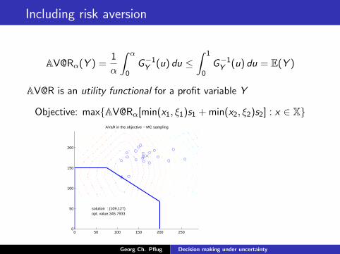
Including risk aversion
AV@Rα(Y ) =1
α
∫ α
0G−1Y (u) du ≤
∫ 1
0G−1Y (u) du = E(Y )
AV@R is an utility functional for a profit variable Y
Objective: maxAV@Rα[min(x1, ξ1)s1 +min(x2, ξ2)s2] : x ∈ X
0 50 100 150 200 2500
50
100
150
200
AVaR in the objective − MC sampling
solution : (109,127)opt. value:345.7933
Georg Ch. Pflug Decision making under uncertainty
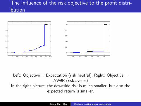
The influence of the risk objective to the profit distri-bution
50 100 150 200 250 300 350 400 450
0
0.2
0.4
0.6
0.8
1
240 260 280 300 320 340
0
0.2
0.4
0.6
0.8
1
Left: Objective = Expectation (risk neutral), Right: Objective =AV@R (risk averse)
In the right picture, the downside risk is much smaller, but also theexpected return is smaller.
Georg Ch. Pflug Decision making under uncertainty
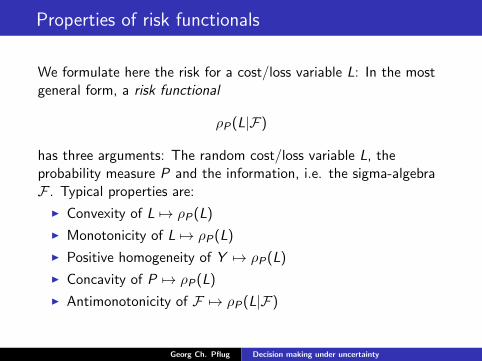
Properties of risk functionals
We formulate here the risk for a cost/loss variable L: In the mostgeneral form, a risk functional
ρP(L|F)
has three arguments: The random cost/loss variable L, theprobability measure P and the information, i.e. the sigma-algebraF . Typical properties are:
I Convexity of L 7→ ρP(L)
I Monotonicity of L 7→ ρP(L)
I Positive homogeneity of Y 7→ ρP(L)
I Concavity of P 7→ ρP(L)
I Antimonotonicity of F 7→ ρP(L|F)
Georg Ch. Pflug Decision making under uncertainty
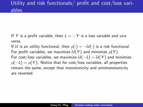
Utility and risk functionals/ profit and cost/loss vari-ables
If Y is a profit variable, then L = −Y is a loss variable and viceversa.If U is an utility functional, then ρ(·) = −U(·) is a risk functional.For profit variables, we maximize U(Y ) and minimize ρ(Y ).For cost/loss variables, we maximize U(−L) = U(Y ) and minimizeρ(−L) = ρ(Y ). Notice that for cost/loss variables, all propertiesremain the same, except that monotonicity and antimonotonicityare reversed.
Georg Ch. Pflug Decision making under uncertainty
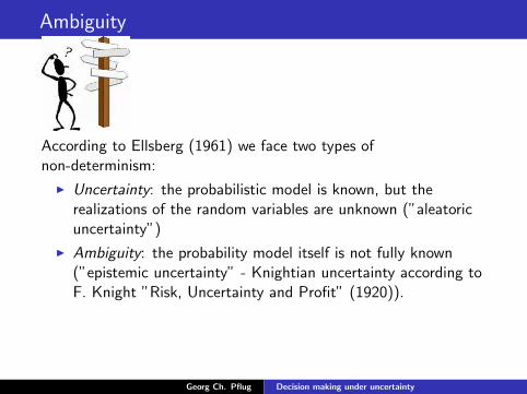
Ambiguity
According to Ellsberg (1961) we face two types ofnon-determinism:
I Uncertainty: the probabilistic model is known, but therealizations of the random variables are unknown (”aleatoricuncertainty”)
I Ambiguity: the probability model itself is not fully known(”epistemic uncertainty” - Knightian uncertainty according toF. Knight ”Risk, Uncertainty and Profit” (1920)).
Georg Ch. Pflug Decision making under uncertainty
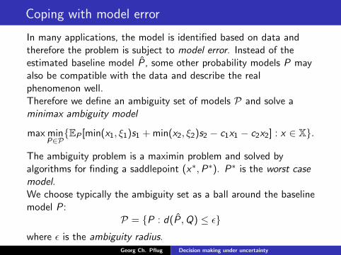
Coping with model error
In many applications, the model is identified based on data andtherefore the problem is subject to model error. Instead of theestimated baseline model P, some other probability models P mayalso be compatible with the data and describe the realphenomenon well.Therefore we define an ambiguity set of models P and solve aminimax ambiguity model
max minP∈P
EP [min(x1, ξ1)s1 +min(x2, ξ2)s2 − c1x1 − c2x2] : x ∈ X.
The ambiguity problem is a maximin problem and solved byalgorithms for finding a saddlepoint (x∗,P∗). P∗ is the worst casemodel.We choose typically the ambiguity set as a ball around the baselinemodel P:
P = P : d(P,Q) ≤ ϵwhere ϵ is the ambiguity radius.
Georg Ch. Pflug Decision making under uncertainty
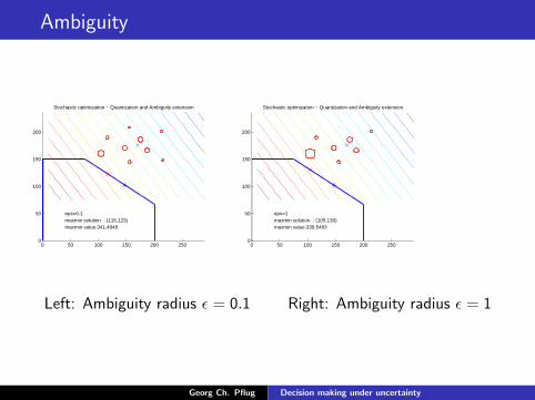
Ambiguity
0 50 100 150 200 2500
50
100
150
200
Stochastic optimization − Quantization and Ambiguity extension
eps=0.1maxmin solution : (116,123)maxmin value:341.4948
0 50 100 150 200 2500
50
100
150
200
Stochastic optimization − Quantization and Ambiguity extension
eps=1maxmin solution : (105,130)maxmin value:339.5483
Left: Ambiguity radius ϵ = 0.1 Right: Ambiguity radius ϵ = 1
Georg Ch. Pflug Decision making under uncertainty
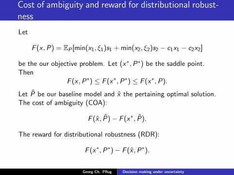
Cost of ambiguity and reward for distributional robust-ness
Let
F (x ,P) = EP [min(x1, ξ1)s1 +min(x2, ξ2)s2 − c1x1 − c2x2]
be the our objective problem. Let (x∗,P∗) be the saddle point.Then
F (x ,P∗) ≤ F (x∗,P∗) ≤ F (x∗,P).
Let P be our baseline model and x the pertaining optimal solution.The cost of ambiguity (COA):
F (x , P)− F (x∗, P).
The reward for distributional robustness (RDR):
F (x∗,P∗)− F (x ,P∗).
Georg Ch. Pflug Decision making under uncertainty
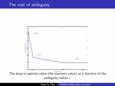
The cost of ambiguity
0.05 0.175 0.275335
340
345
350
355
360
365
Ambiguity Radius
Max
imin
Obj
ectiv
e V
alue
339.54
361.85
343.38
The drop in optimal value (the maximin value) as a function of theambiguity radius ϵ.
Georg Ch. Pflug Decision making under uncertainty
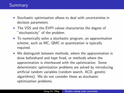
Summary
I Stochastic optimization allows to deal with uncertainties indecision parameters.
I The VSS and the EVPI values characterize the degree of”stochasticity” of the problem.
I To numerically solve a stochastic program, an approximationscheme, such as MC, QMC or quantization is typicallyrequired.
I We distinguish between methods, where the approximation isdone beforehand and kept fixed, or methods where theapproximation is interleaved with the optimization. Somedeterministic optimization problems are solved by introducingartificial random variables (random search, ACO, geneticalgorithms). We do not consider these as stochasticoptimization problems.
Georg Ch. Pflug Decision making under uncertainty
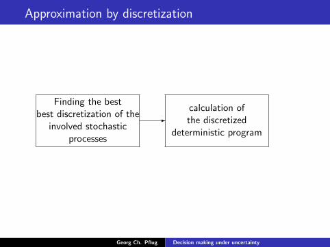
Approximation by discretization
Finding the bestbest discretization of the
involved stochasticprocesses
-calculation ofthe discretized
deterministic program
Georg Ch. Pflug Decision making under uncertainty
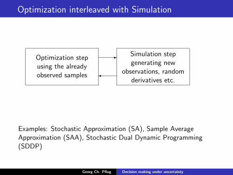
Optimization interleaved with Simulation
Optimization stepusing the alreadyobserved samples
-
Simulation stepgenerating new
observations, randomderivatives etc.
Examples: Stochastic Approximation (SA), Sample AverageApproximation (SAA), Stochastic Dual Dynamic Programming(SDDP)
Georg Ch. Pflug Decision making under uncertainty
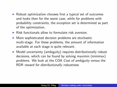
I Robust optimization chooses first a typical set of outcomesand looks then for the worst case, while for problems withprobability constraints, the exception set is determined as partof the optimization.
I Risk functionals allow to formulate risk aversion.
I More sophisticated decision problems are stochasticmulti-stage. For these problems, the amount of informationavailable at each stage is quite relevant.
I Model uncertainty (ambiguity) requires distributionally robustdecisions, which can be found by solving maximin (minimax)problems. We look at the COA Cost of ambiguity versus theRDR reward for distributionally robustness
Georg Ch. Pflug Decision making under uncertainty
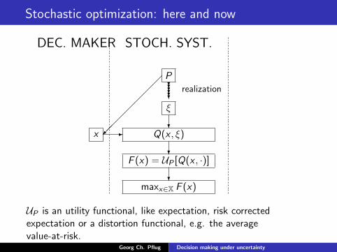
Stochastic optimization: here and now
DEC. MAKER STOCH. SYST.
x Q(x , ξ)
F (x) = UP [Q(x , ·)]
maxx∈X F (x)
P
ξ
??????realization
?
?
?
-
UP is an utility functional, like expectation, risk correctedexpectation or a distortion functional, e.g. the averagevalue-at-risk.
Georg Ch. Pflug Decision making under uncertainty
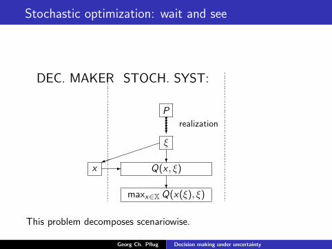
Stochastic optimization: wait and see
DEC. MAKER STOCH. SYST:
x Q(x , ξ)
maxx∈XQ(x(ξ), ξ)
P
ξ
??????realization
?
?
-
)
This problem decomposes scenariowise.
Georg Ch. Pflug Decision making under uncertainty
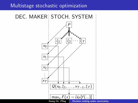
Multistage stochastic optimization
DEC. MAKER STOCH. SYSTEM
x0
x1
x2
...xT
ξ1 ξ2 · · · ξT
P
Q(x0, ξ1, . . . , xT−1, ξT )
maxx F (x) = UP [f (...)]
????????jjjjjjjj
?
? ? ? ?
Georg Ch. Pflug Decision making under uncertainty
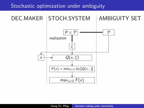
Stochastic optimization under ambiguity
DEC.MAKER STOCH.SYSTEM AMBIGUITY SET
x Q(x , ξ)
F (x) = minP∈P UP [Q(x , ·)]
maxx∈X F (x)
P ∈ P
ξ
??????realization
?
?
?
-
P
?
Georg Ch. Pflug Decision making under uncertainty
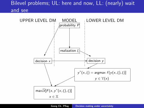
Bilevel problems; UL: here and now, LL: (nearly) waitand see
UPPER LEVEL DM MODEL LOWER LEVEL DMprobability P
realization ξ
decision x decision y
y∗(x , ξ) = argmax f (y(x , ξ), ξ)]
y ∈ Y(x)
maxU [F (x , y∗(x , ξ), ξ)]
x ∈ X
?
HHHj-
BBBBBBN
Georg Ch. Pflug Decision making under uncertainty
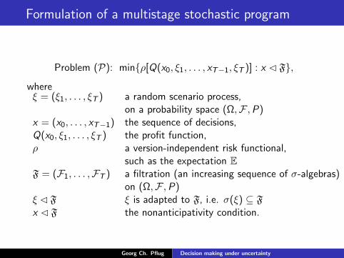
Formulation of a multistage stochastic program
Problem (P): minρ[Q(x0, ξ1, . . . , xT−1, ξT )] : x F,
whereξ = (ξ1, . . . , ξT ) a random scenario process,
on a probability space (Ω,F ,P)x = (x0, . . . , xT−1) the sequence of decisions,Q(x0, ξ1, . . . , ξT ) the profit function,ρ a version-independent risk functional,
such as the expectation EF = (F1, . . . ,FT ) a filtration (an increasing sequence of σ-algebras)
on (Ω,F ,P)ξ F ξ is adapted to F, i.e. σ(ξ) ⊆ Fx F the nonanticipativity condition.
Georg Ch. Pflug Decision making under uncertainty
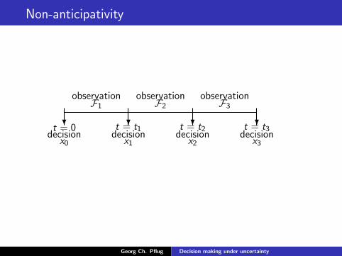
Non-anticipativity
? ? ? ?decision decision decision decision
x0 x1 x2 x3
t = 0 t = t1 t = t2 t = t3
observation observation observationF1 F2 F3
Georg Ch. Pflug Decision making under uncertainty
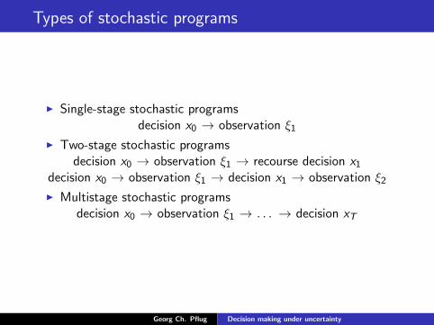
Types of stochastic programs
I Single-stage stochastic programsdecision x0 → observation ξ1
I Two-stage stochastic programsdecision x0 → observation ξ1 → recourse decision x1
decision x0 → observation ξ1 → decision x1 → observation ξ2
I Multistage stochastic programsdecision x0 → observation ξ1 → . . . → decision xT
Georg Ch. Pflug Decision making under uncertainty
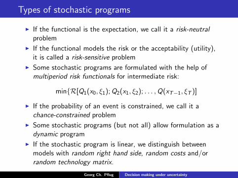
Types of stochastic programs
I If the functional is the expectation, we call it a risk-neutralproblem
I If the functional models the risk or the acceptability (utility),it is called a risk-sensitive problem
I Some stochastic programs are formulated with the help ofmultiperiod risk functionals for intermediate risk:
minR[Q1(x0, ξ1);Q2(x1, ξ2); . . . ,Q(xT−1, ξT )]
I If the probability of an event is constrained, we call it achance-constrained problem
I Some stochastic programs (but not all) allow formulation as adynamic program
I If the stochastic program is linear, we distinguish betweenmodels with random right hand side, random costs and/orrandom technology matrix.
Georg Ch. Pflug Decision making under uncertainty
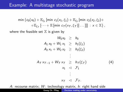
Example: A multistage stochastic program
min c0(x0) + Eξ1 [min c1(x1, ξ1) + Eξ2 [min c2(x2, ξ2)+
+EξT [· · ·+ E [min cT (xT , ξT )] . . . ]]] : x ∈ X ,where the feasible set X is given by
W0x0 ≥ h0
A1 x0 +W1 x1 ≥ h1(ξ1)
A2 x1 +W2 x2 ≥ h2(ξ2)...
AT xT−1 +WT xT ≥ hT (ξT ) (4)
x1 F1
...
xT FT .
A: recourse matrix; W : technology matrix, h: right hand sideGeorg Ch. Pflug Decision making under uncertainty
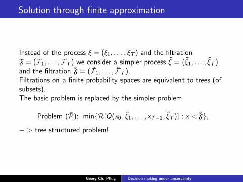
Solution through finite approximation
Instead of the process ξ = (ξ1, . . . , ξT ) and the filtrationF = (F1, . . . ,FT ) we consider a simpler process ξ = (ξ1, . . . , ξT )and the filtration F = (F1, . . . , FT ).Filtrations on a finite probability spaces are equivalent to trees (ofsubsets).The basic problem is replaced by the simpler problem
Problem (P): minR[Q(x0, ξ1, . . . , xT−1, ξT )] : x F,
− > tree structured problem!
Georg Ch. Pflug Decision making under uncertainty
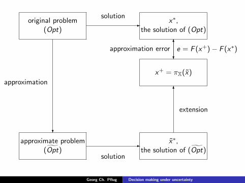
approximate problem(Opt)
original problem(Opt)
x∗,the solution of (Opt)
x+ = πX(x)
x∗,the solution of (Opt)
?
-
-
6
6
?
solution
solution
approximation
extension
approximation error e = F (x+)− F (x∗)
Georg Ch. Pflug Decision making under uncertainty
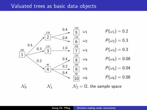
Valuated trees as basic data objects
:0.4
5130
ω1 P(ω1) = 0.2
XXXXXz0.6
6110
ω2 P(ω2) = 0.3
-1.07105
ω3 P(ω3) = 0.3
*0.4 8
115
ω4 P(ω4) = 0.08
-0.29100
ω5 P(ω5) = 0.04HHHHHj0.4
1090
ω6 P(ω6) = 0.08
0.5
2120
:0.3
3110
ZZZZZ~
0.2
490
1100
N0 N1 N2 = Ω, the sample space
Georg Ch. Pflug Decision making under uncertainty
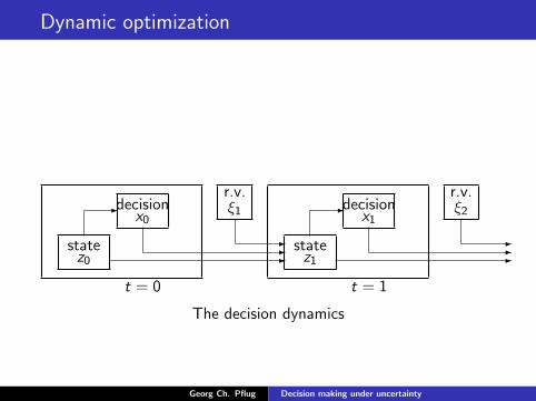
Dynamic optimization
statez0
decisionx0
r.v.ξ1
statez1
decisionx1
r.v.ξ2-
---
-
---
t = 0 t = 1
The decision dynamics
Georg Ch. Pflug Decision making under uncertainty
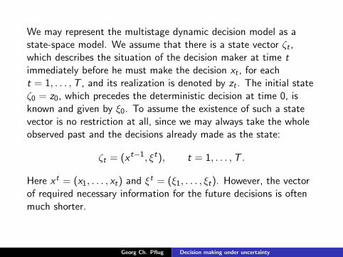
We may represent the multistage dynamic decision model as astate-space model. We assume that there is a state vector ζt ,which describes the situation of the decision maker at time timmediately before he must make the decision xt , for eacht = 1, . . . ,T , and its realization is denoted by zt . The initial stateζ0 = z0, which precedes the deterministic decision at time 0, isknown and given by ξ0. To assume the existence of such a statevector is no restriction at all, since we may always take the wholeobserved past and the decisions already made as the state:
ζt = (x t−1, ξt), t = 1, . . . ,T .
Here x t = (x1, . . . , xt) and ξt = (ξ1, . . . , ξt). However, the vectorof required necessary information for the future decisions is oftenmuch shorter.
Georg Ch. Pflug Decision making under uncertainty
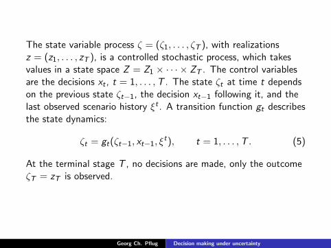
The state variable process ζ = (ζ1, . . . , ζT ), with realizationsz = (z1, . . . , zT ), is a controlled stochastic process, which takesvalues in a state space Z = Z1 × · · · × ZT . The control variablesare the decisions xt , t = 1, . . . ,T . The state ζt at time t dependson the previous state ζt−1, the decision xt−1 following it, and thelast observed scenario history ξt . A transition function gt describesthe state dynamics:
ζt = gt(ζt−1, xt−1, ξt), t = 1, . . . ,T . (5)
At the terminal stage T , no decisions are made, only the outcomeζT = zT is observed.
Georg Ch. Pflug Decision making under uncertainty
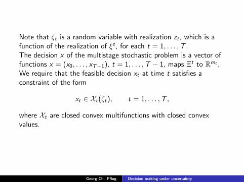
Note that ζt is a random variable with realization zt , which is afunction of the realization of ξt , for each t = 1, . . . ,T .The decision x of the multistage stochastic problem is a vector offunctions x = (x0, . . . , xT−1), t = 1, . . . ,T − 1, maps Ξt to Rmt .We require that the feasible decision xt at time t satisfies aconstraint of the form
xt ∈ Xt(ζt), t = 1, . . . ,T ,
where Xt are closed convex multifunctions with closed convexvalues.
Georg Ch. Pflug Decision making under uncertainty
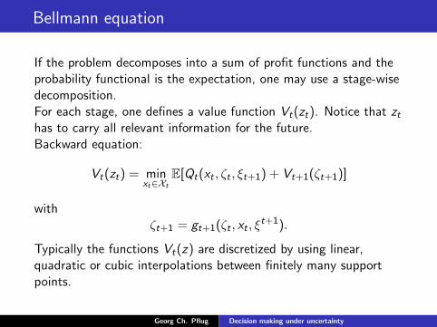
Bellmann equation
If the problem decomposes into a sum of profit functions and theprobability functional is the expectation, one may use a stage-wisedecomposition.For each stage, one defines a value function Vt(zt). Notice that zthas to carry all relevant information for the future.Backward equation:
Vt(zt) = minxt∈Xt
E[Qt(xt , ζt , ξt+1) + Vt+1(ζt+1)]
withζt+1 = gt+1(ζt , xt , ξ
t+1).
Typically the functions Vt(z) are discretized by using linear,quadratic or cubic interpolations between finitely many supportpoints.
Georg Ch. Pflug Decision making under uncertainty
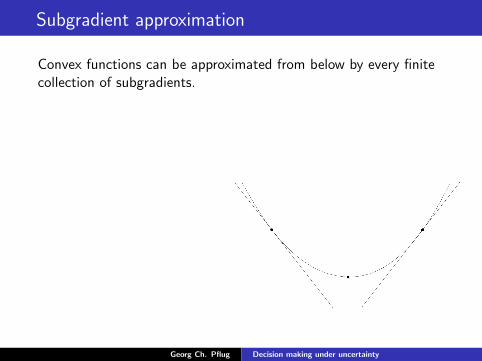
Subgradient approximation
Convex functions can be approximated from below by every finitecollection of subgradients.
Georg Ch. Pflug Decision making under uncertainty
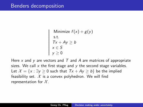
Benders decomposition
∥∥∥∥∥∥∥∥∥∥Minimize f (x) + g(y)s.t.Tx + Ay ≥ bx ∈ Sy ≥ 0
Here x and y are vectors and T and A are matrices of appropriatesizes. We call x the first stage and y the second stage variables.Let X = x : ∃y ≥ 0 such that Tx + Ay ≥ b be the impliedfeasibility set. X is a convex polyhedron. We will findrepresentation for X .
Georg Ch. Pflug Decision making under uncertainty
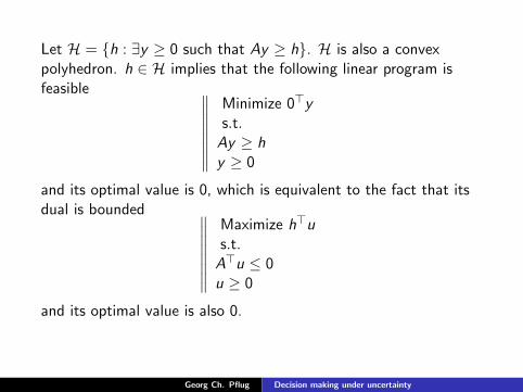
Let H = h : ∃y ≥ 0 such that Ay ≥ h. H is also a convexpolyhedron. h ∈ H implies that the following linear program isfeasible ∥∥∥∥∥∥∥∥
Minimize 0⊤ys.t.Ay ≥ hy ≥ 0
and its optimal value is 0, which is equivalent to the fact that itsdual is bounded ∥∥∥∥∥∥∥∥
Maximize h⊤us.t.A⊤u ≤ 0u ≥ 0
and its optimal value is also 0.
Georg Ch. Pflug Decision making under uncertainty
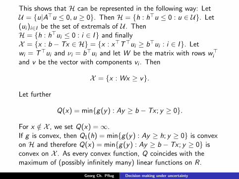
This shows that H can be represented in the following way: LetU = u|A⊤u ≤ 0, u ≥ 0. Then H = h : h⊤u ≤ 0 : u ∈ U. Let(ui )i∈I be the set of extremals of U . ThenH = h : h⊤ui ≤ 0 : i ∈ I and finallyX = x : b − Tx ∈ H = x : x⊤T⊤ui ≥ b⊤ui : i ∈ I. Letwi = T⊤ui and νi = b⊤ui and let W be the matrix with rows w⊤
i
and v be the vector with components vi . Then
X = x : Wx ≥ v.
Let further
Q(x) = ming(y) : Ay ≥ b − Tx ; y ≥ 0.
For x /∈ X , we set Q(x) = ∞.If g is convex, then Q1(h) = ming(y) : Ay ≥ h; y ≥ 0 is convexon H and therefore Q(x) = ming(y) : Ay ≥ b − Tx ; y ≥ 0 isconvex on X . As every convex function, Q coincides with themaximum of (possibly infinitely many) linear functions on R.
Georg Ch. Pflug Decision making under uncertainty
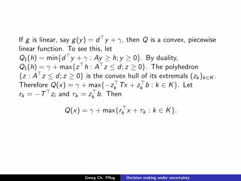
If g is linear, say g(y) = d⊤y + γ, then Q is a convex, piecewiselinear function. To see this, letQ1(h) = mind⊤y + γ : Ay ≥ h; y ≥ 0. By duality,Q1(h) = γ +maxz⊤h : A⊤z ≤ d ; z ≥ 0. The polyhedronz : A⊤z ≤ d ; z ≥ 0 is the convex hull of its extremals (zk)k∈K .Therefore Q(x) = γ +max−z⊤k Tx + z⊤k b : k ∈ K. Letrk = −T⊤zi and τk = z⊤k b. Then
Q(x) = γ +maxr⊤k x + τk : k ∈ K.
Georg Ch. Pflug Decision making under uncertainty
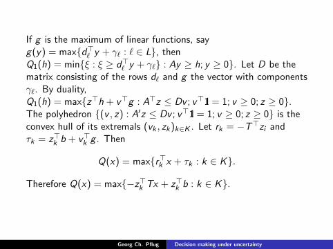
If g is the maximum of linear functions, sayg(y) = maxd⊤
ℓ y + γℓ : ℓ ∈ L, thenQ1(h) = minξ : ξ ≥ d⊤
ℓ y + γℓ : Ay ≥ h; y ≥ 0. Let D be thematrix consisting of the rows dℓ and g the vector with componentsγℓ. By duality,Q1(h) = maxz⊤h + v⊤g : A⊤z ≤ Dv ; v⊤1l = 1; v ≥ 0; z ≥ 0.The polyhedron (v , z) : A′z ≤ Dv ; v⊤1l = 1; v ≥ 0; z ≥ 0 is theconvex hull of its extremals (vk , zk)k∈K . Let rk = −T⊤zi andτk = z⊤k b + v⊤k g . Then
Q(x) = maxr⊤k x + τk : k ∈ K.
Therefore Q(x) = max−z⊤k Tx + z⊤k b : k ∈ K.
Georg Ch. Pflug Decision making under uncertainty
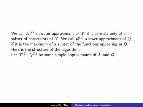
We call X (s) an outer approximant of X , if it consists only of asubset of constraints of X . We call Q(s) a lower approximant of Q,if it is the maximum of a subset of the functions appearing in Q.Here is the structure of the algorithm.Let X (1), Q(1) be some simple approximants of X and Q.
Georg Ch. Pflug Decision making under uncertainty
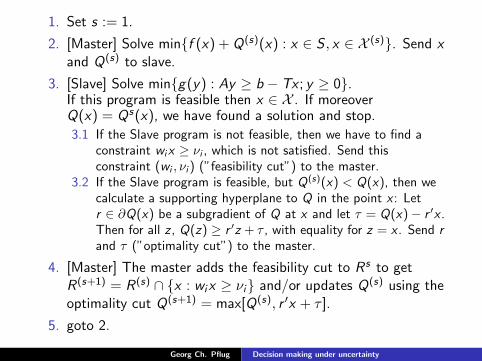
1. Set s := 1.
2. [Master] Solve minf (x) +Q(s)(x) : x ∈ S , x ∈ X (s). Send xand Q(s) to slave.
3. [Slave] Solve ming(y) : Ay ≥ b − Tx ; y ≥ 0.If this program is feasible then x ∈ X . If moreoverQ(x) = Qs(x), we have found a solution and stop.
3.1 If the Slave program is not feasible, then we have to find aconstraint wix ≥ νi , which is not satisfied. Send thisconstraint (wi , νi ) (”feasibility cut”) to the master.
3.2 If the Slave program is feasible, but Q(s)(x) < Q(x), then wecalculate a supporting hyperplane to Q in the point x : Letr ∈ ∂Q(x) be a subgradient of Q at x and let τ = Q(x)− r ′x .Then for all z , Q(z) ≥ r ′z + τ , with equality for z = x . Send rand τ (”optimality cut”) to the master.
4. [Master] The master adds the feasibility cut to Rs to getR(s+1) = R(s) ∩ x : wix ≥ νi and/or updates Q(s) using theoptimality cut Q(s+1) = max[Q(s), r ′x + τ ].
5. goto 2.
Georg Ch. Pflug Decision making under uncertainty
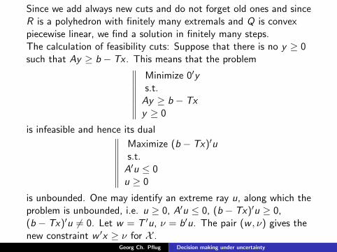
Since we add always new cuts and do not forget old ones and sinceR is a polyhedron with finitely many extremals and Q is convexpiecewise linear, we find a solution in finitely many steps.The calculation of feasibility cuts: Suppose that there is no y ≥ 0such that Ay ≥ b − Tx . This means that the problem∥∥∥∥∥∥∥∥
Minimize 0′ys.t.Ay ≥ b − Txy ≥ 0
is infeasible and hence its dual∥∥∥∥∥∥∥∥Maximize (b − Tx)′us.t.A′u ≤ 0u ≥ 0
is unbounded. One may identify an extreme ray u, along which theproblem is unbounded, i.e. u ≥ 0, A′u ≤ 0, (b − Tx)′u ≥ 0,(b − Tx)′u = 0. Let w = T ′u, ν = b′u. The pair (w , ν) gives thenew constraint w ′x ≥ ν for X .
Georg Ch. Pflug Decision making under uncertainty
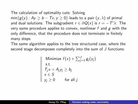
The calculation of optimality cuts: Solvingming(y) : Ay ≥ b − Tx ; y ≥ 0 leads to a pair (y , λ) of primaland dual solutions. The subgradient r ∈ ∂Q(x) is r = −T ′λ. Thevery same procedure applies to convex, nonlinear f and g with theonly difference, that the procedure does not terminate in finitelymany steps.The same algorithm applies to the tree structured case, where thesecond stage decomposes completely into the sum of J functions:∥∥∥∥∥∥∥∥∥∥
Minimize f (x) +∑J
j=1 gj(yj)
s.t.Tjx + Ajyj ≥ bjx ∈ Syj ≥ 0 for all j
Georg Ch. Pflug Decision making under uncertainty

flow of primal information flow of dual information (solutions passed to successor nodes) (feasibility and optimality cuts passed to predecessor nodes)
Georg Ch. Pflug Decision making under uncertainty
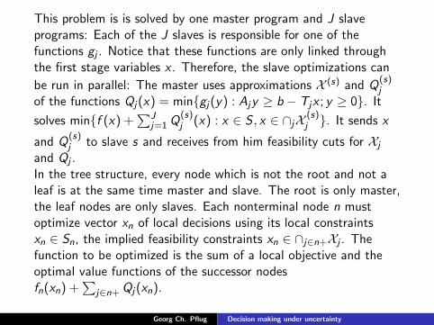
This problem is is solved by one master program and J slaveprograms: Each of the J slaves is responsible for one of thefunctions gj . Notice that these functions are only linked throughthe first stage variables x . Therefore, the slave optimizations can
be run in parallel: The master uses approximations X (s) and Q(s)j
of the functions Qj(x) = mingj(y) : Ajy ≥ b − Tjx ; y ≥ 0. Itsolves minf (x) +
∑Jj=1Q
(s)j (x) : x ∈ S , x ∈ ∩jX (s)
j . It sends xand Q
(s)j to slave s and receives from him feasibility cuts for Xj
and Qj .In the tree structure, every node which is not the root and not aleaf is at the same time master and slave. The root is only master,the leaf nodes are only slaves. Each nonterminal node n mustoptimize vector xn of local decisions using its local constraintsxn ∈ Sn, the implied feasibility constraints xn ∈ ∩j∈n+Xj . Thefunction to be optimized is the sum of a local objective and theoptimal value functions of the successor nodesfn(xn) +
∑j∈n+Qj(xn).
Georg Ch. Pflug Decision making under uncertainty
SDDP- Pereira
The SDDP approach is identical to the Benders decomposition,but does not construct the scenario tree right from the beginning,but uses values of the process which are sampled in during theprocedure.If the stochastic process ξ is independent, then this method is veryefficient, since no conditional distributions appear. However, theindependence assumption is very questionable and to modify theprocess in such a way that only independent innovations appear isnot always possible.
Georg Ch. Pflug Decision making under uncertainty
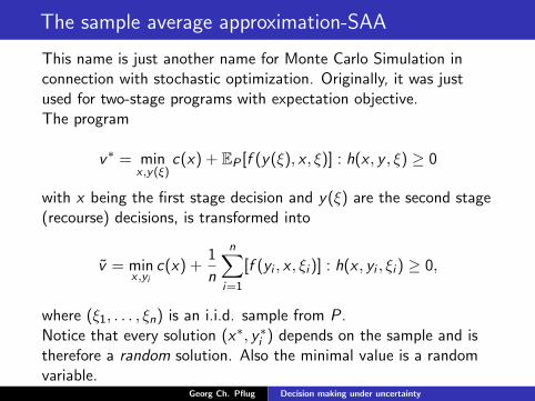
The sample average approximation-SAA
This name is just another name for Monte Carlo Simulation inconnection with stochastic optimization. Originally, it was justused for two-stage programs with expectation objective.The program
v∗ = minx ,y(ξ)
c(x) + EP [f (y(ξ), x , ξ)] : h(x , y , ξ) ≥ 0
with x being the first stage decision and y(ξ) are the second stage(recourse) decisions, is transformed into
v = minx ,yi
c(x) +1
n
n∑i=1
[f (yi , x , ξi )] : h(x , yi , ξi ) ≥ 0,
where (ξ1, . . . , ξn) is an i.i.d. sample from P.Notice that every solution (x∗, y∗i ) depends on the sample and istherefore a random solution. Also the minimal value is a randomvariable.
Georg Ch. Pflug Decision making under uncertainty
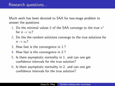
Research questions...
Much work has been devoted to SAA for two-stage problem toanswer the questions
1. Do the minimal values v of the SAA converge to the true v∗
for n → ∞?
2. Do the the random solutions converge to the true solutions forn → ∞?
3. How fast is the convergence in 1.?
4. How fast is the convergence in 2.?
5. Is there asymptotic normality in 1. and can one getconfidence intervals for the true solution?
6. Is there asymptotic normality in 2. and can one getconfidence intervals for the true solution?
Georg Ch. Pflug Decision making under uncertainty
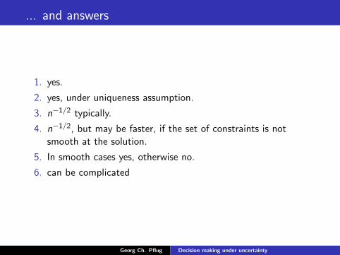
... and answers
1. yes.
2. yes, under uniqueness assumption.
3. n−1/2 typically.
4. n−1/2, but may be faster, if the set of constraints is notsmooth at the solution.
5. In smooth cases yes, otherwise no.
6. can be complicated
Georg Ch. Pflug Decision making under uncertainty
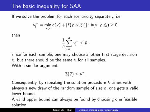
The basic inequality for SAA
If we solve the problem for each scenario ξi separately, i.e.
v+i = minx ,y
c(x) + [f (y , x , ξi )] : h(x , y , ξi ) ≥ 0
then1
n
n∑i=1
v+i ≤ v .
since for each sample, one may choose another first stage decisionx , but there should be the same x for all samples.With a similar argument
E(v) ≤ v∗.
Consequently, by repeating the solution procedure k times withalways a new draw of the random sample of size n, one gets a validlower bound.A valid upper bound can always be found by choosing one feasiblesolution.
Georg Ch. Pflug Decision making under uncertainty
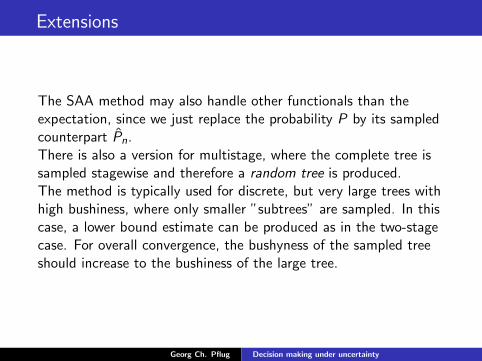
Extensions
The SAA method may also handle other functionals than theexpectation, since we just replace the probability P by its sampledcounterpart Pn.There is also a version for multistage, where the complete tree issampled stagewise and therefore a random tree is produced.The method is typically used for discrete, but very large trees withhigh bushiness, where only smaller ”subtrees” are sampled. In thiscase, a lower bound estimate can be produced as in the two-stagecase. For overall convergence, the bushyness of the sampled treeshould increase to the bushiness of the large tree.
Georg Ch. Pflug Decision making under uncertainty