Embed Size (px)
Citation preview
GeoPDEsAn Octave/Matlab software for research on IGA
R. Vazquez
IMATI ‘Enrico Magenes’, Pavia
Consiglio Nazionale della Ricerca
Joint work withC. de Falco and A. Reali
Supported by the ERC Starting Grant:GeoPDEs n. 205004
R. Vazquez (IMATI-CNR Italy) GeoPDEs: a research tool for IGA IGA school, Cetraro, 2012 1 / 22
1 Motivation
2 IGA in an abstract framework
3 The implementation of GeoPDEsThe parameterization: geometry structureThe quadrature rule: mesh structureThe discrete space: space structureBoundary conditions: the boundary substructures
4 Some simple examplesPoisson equationLinear elasticityMaxwell equations
R. Vazquez (IMATI-CNR Italy) GeoPDEs: a research tool for IGA IGA school, Cetraro, 2012 2 / 22
Motivation
We wanted to share our codes with people interested on IGA.
Starting point: different codes, different problems, different developers.
Primary goal: uniform implementation of our different codes.
The result is GeoPDEs: open and free software for IGA.
The software is implemented in Octave, fully compatible with Matlab.
Very clear for teaching purposes.
Easy to modify and to use for fast prototyping.
Follows an abstract setting to cover many problems and methods.
Secondary goal: faster and more efficient implementation.
Important advances in GeoPDEs 2.0 (last part of the talk).
R. Vazquez (IMATI-CNR Italy) GeoPDEs: a research tool for IGA IGA school, Cetraro, 2012 3 / 22
General description of the software
GeoPDEs consists of a set of interrelated packages for different problems:
base: the main package, with examples for Laplace problem.
elasticity: a simple package for linear elasticity problems.
fluid: Stokes’ equations, with different choices for the discrete spaces.
maxwell: Maxwell equations, generalization of edge finite elements.
multipatch: extension to multi-patch defined geometries.
The main structures and functions are defined in the base package.
The other packages are based on the structures defined in base.
The nomenclature is mostly the same in every package.
We define IGA in an abstract way, to cover as many cases as possible.
R. Vazquez (IMATI-CNR Italy) GeoPDEs: a research tool for IGA IGA school, Cetraro, 2012 4 / 22
IGA in an abstract framework
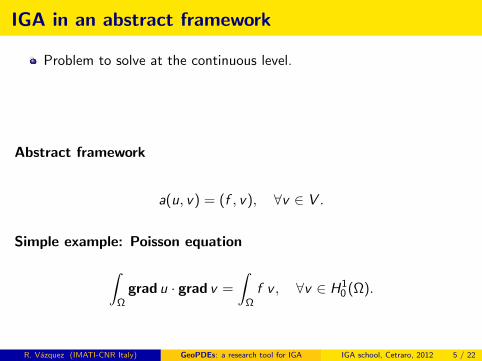
Problem to solve at the continuous level.
Parametric domain and parameterization of the physical domain.
Discrete problem and spaces in the parametric and physical domain.
Construct and solve a linear system to find the discrete solution.
Abstract framework
a(u, v) = (f , v), ∀v ∈ V .
Simple example: Poisson equation∫Ω
grad u · grad v =
∫Ω
f v , ∀v ∈ H10 (Ω).
R. Vazquez (IMATI-CNR Italy) GeoPDEs: a research tool for IGA IGA school, Cetraro, 2012 5 / 22
IGA in an abstract framework
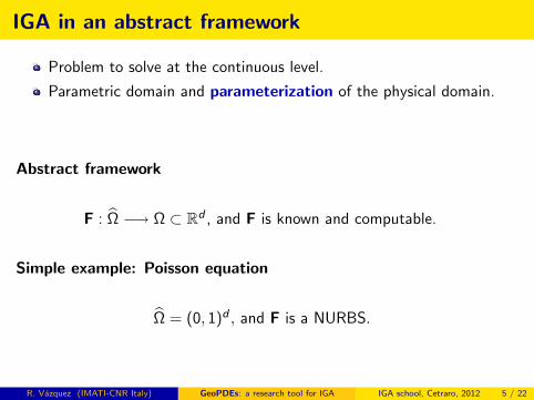
Problem to solve at the continuous level.
Parametric domain and parameterization of the physical domain.
Discrete problem and spaces in the parametric and physical domain.
Construct and solve a linear system to find the discrete solution.
Abstract framework
F : Ω −→ Ω ⊂ Rd , and F is known and computable.
Simple example: Poisson equation
Ω = (0, 1)d , and F is a NURBS.
R. Vazquez (IMATI-CNR Italy) GeoPDEs: a research tool for IGA IGA school, Cetraro, 2012 5 / 22
IGA in an abstract framework
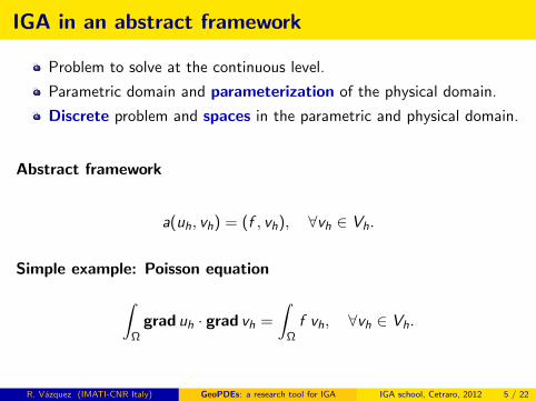
Problem to solve at the continuous level.
Parametric domain and parameterization of the physical domain.
Discrete problem and spaces in the parametric and physical domain.
Construct and solve a linear system to find the discrete solution.
Abstract framework
a(uh, vh) = (f , vh), ∀vh ∈ Vh.
Simple example: Poisson equation∫Ω
grad uh · grad vh =
∫Ω
f vh, ∀vh ∈ Vh.
R. Vazquez (IMATI-CNR Italy) GeoPDEs: a research tool for IGA IGA school, Cetraro, 2012 5 / 22
IGA in an abstract framework
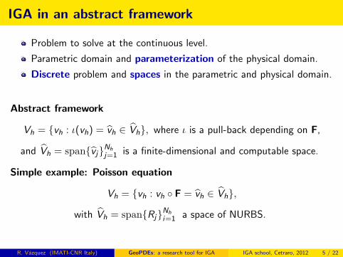
Problem to solve at the continuous level.
Parametric domain and parameterization of the physical domain.
Discrete problem and spaces in the parametric and physical domain.
Construct and solve a linear system to find the discrete solution.
Abstract framework
Vh = vh : ι(vh) = vh ∈ Vh, where ι is a pull-back depending on F,
and Vh = spanvjNhj=1 is a finite-dimensional and computable space.
Simple example: Poisson equation
Vh = vh : vh F = vh ∈ Vh,
with Vh = spanRjNhi=1 a space of NURBS.
R. Vazquez (IMATI-CNR Italy) GeoPDEs: a research tool for IGA IGA school, Cetraro, 2012 5 / 22
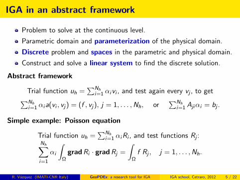
IGA in an abstract framework
Problem to solve at the continuous level.
Parametric domain and parameterization of the physical domain.
Discrete problem and spaces in the parametric and physical domain.
Construct and solve a linear system to find the discrete solution.
Abstract framework
Trial function uh =∑Nh
i=1 αivi , and test again every vj , to get∑Nhi=1 αia(vi , vj) = (f , vj), j = 1, . . . ,Nh, or
∑Nhi=1 Ajiαi = bj .
Simple example: Poisson equation
Trial function uh =∑Nh
i=1 αiRi , and test functions Rj :Nh∑i=1
αi
∫Ω
grad Ri · grad Rj =
∫Ω
f Rj , j = 1, . . . ,Nh.
R. Vazquez (IMATI-CNR Italy) GeoPDEs: a research tool for IGA IGA school, Cetraro, 2012 5 / 22
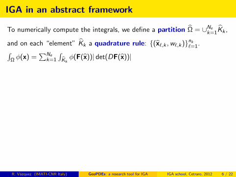
IGA in an abstract framework
To numerically compute the integrals, we define a partition Ω = ∪Nek=1Kk ,
and on each “element” Kk a quadrature rule: (x`,k ,w`,k)nk`=1.∫
Ω φ(x) =∑Ne
k=1
∫bKkφ(F(x))| det(DF(x))|
Using the quadrature rule, the stiffness matrix is computed as
Aij 'Ne∑
k=1
nk∑`=1
w`,k grad vj(F(x`,k)) · grad vi (F(x`,k)) | det(DF(x`,k))|
And recall that grad vi (F(x`,k)) = DF−T grad vi (x`,k).
Summarizing, what we need is
A partition of Ω and a quadrature rule (nodes and weights).
The evaluation of F and the Jacobian DF at the quadrature points.
Value of the shape functions at the “mapped” quadrature points.
A routine to put everything together and compute the matrices.
R. Vazquez (IMATI-CNR Italy) GeoPDEs: a research tool for IGA IGA school, Cetraro, 2012 6 / 22
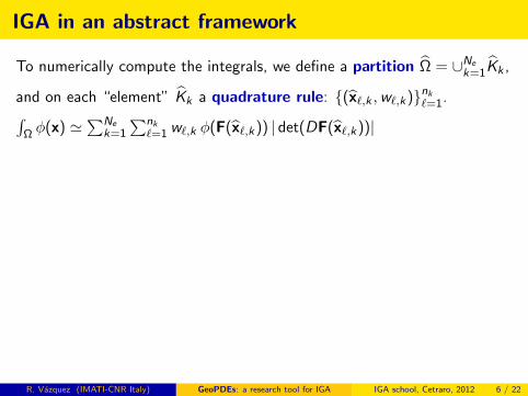
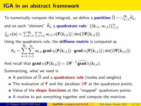
IGA in an abstract framework
To numerically compute the integrals, we define a partition Ω = ∪Nek=1Kk ,
and on each “element” Kk a quadrature rule: (x`,k ,w`,k)nk`=1.∫
Ω φ(x) '∑Ne
k=1
∑nk`=1 w`,k φ(F(x`,k)) | det(DF(x`,k))|
Using the quadrature rule, the stiffness matrix is computed as
Aij 'Ne∑
k=1
nk∑`=1
w`,k grad vj(F(x`,k)) · grad vi (F(x`,k)) | det(DF(x`,k))|
And recall that grad vi (F(x`,k)) = DF−T grad vi (x`,k).
Summarizing, what we need is
A partition of Ω and a quadrature rule (nodes and weights).
The evaluation of F and the Jacobian DF at the quadrature points.
Value of the shape functions at the “mapped” quadrature points.
A routine to put everything together and compute the matrices.
R. Vazquez (IMATI-CNR Italy) GeoPDEs: a research tool for IGA IGA school, Cetraro, 2012 6 / 22
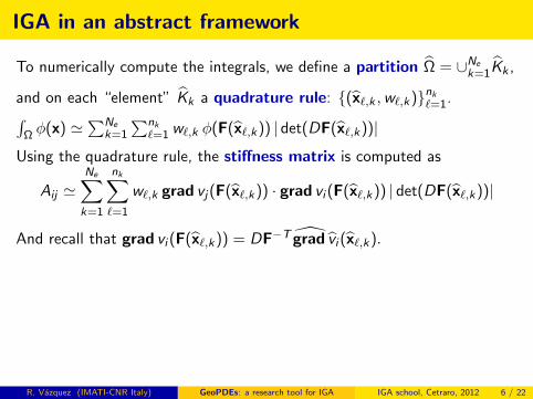
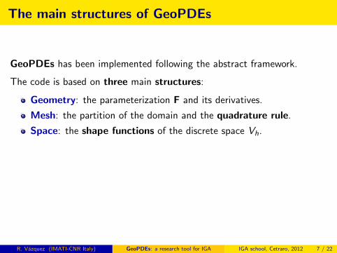
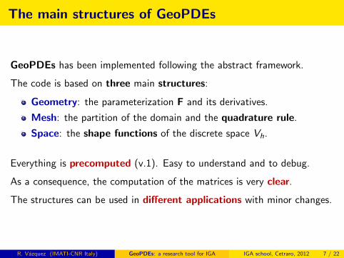
The main structures of GeoPDEs
GeoPDEs has been implemented following the abstract framework.
The code is based on three main structures:
Geometry: the parameterization F and its derivatives.
Mesh: the partition of the domain and the quadrature rule.
Space: the shape functions of the discrete space Vh.
Everything is precomputed (v.1). Easy to understand and to debug.
As a consequence, the computation of the matrices is very clear.
The structures can be used in different applications with minor changes.
R. Vazquez (IMATI-CNR Italy) GeoPDEs: a research tool for IGA IGA school, Cetraro, 2012 7 / 22
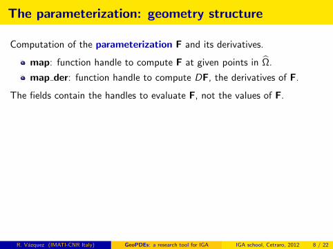
The parameterization: geometry structure
Computation of the parameterization F and its derivatives.
map: function handle to compute F at given points in Ω.
map der: function handle to compute DF, the derivatives of F.
The fields contain the handles to evaluate F, not the values of F.
For NURBS and B-splines, we make use of the NURBS toolbox.
Based on standard NURBS algorithms (see, e.g., the NURBS book).
Useful for simple geometry manipulation (revolution, extrusion,...)
It is also used in GeoPDEs for function evaluation.
The computation of the geometry is separated from the shape functions.
Necessary for non-isoparametric discretizations.
Geometry evaluations can be made in the coarsest given geometry.
R. Vazquez (IMATI-CNR Italy) GeoPDEs: a research tool for IGA IGA school, Cetraro, 2012 8 / 22
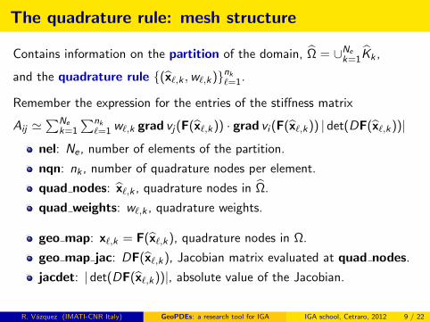
The quadrature rule: mesh structure
Contains information on the partition of the domain, Ω = ∪Nek=1Kk ,
and the quadrature rule (x`,k ,w`,k)nk`=1.
Remember the expression for the entries of the stiffness matrix
Aij '∑Ne
k=1
∑nk`=1 w`,k grad vj(F(x`,k)) · grad vi (F(x`,k)) | det(DF(x`,k))|
nel: Ne , number of elements of the partition.
nqn: nk , number of quadrature nodes per element.
quad nodes: x`,k , quadrature nodes in Ω.
quad weights: w`,k , quadrature weights.
geo map: x`,k = F(x`,k), quadrature nodes in Ω.
geo map jac: DF(x`,k), Jacobian matrix evaluated at quad nodes.
jacdet: | det(DF(x`,k))|, absolute value of the Jacobian.
R. Vazquez (IMATI-CNR Italy) GeoPDEs: a research tool for IGA IGA school, Cetraro, 2012 9 / 22
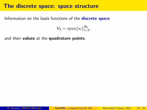
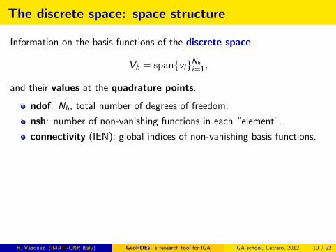
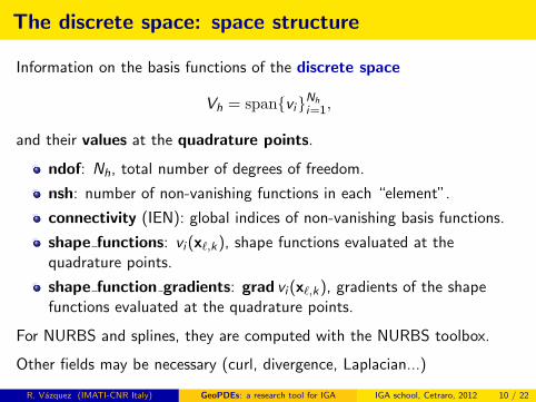
The discrete space: space structure
Information on the basis functions of the discrete space
Vh = spanviNhi=1,
and their values at the quadrature points.
ndof: Nh, total number of degrees of freedom.
nsh: number of non-vanishing functions in each “element”.
connectivity (IEN): global indices of non-vanishing basis functions.
shape functions: vi (x`,k), shape functions evaluated at thequadrature points.
shape function gradients: grad vi (x`,k), gradients of the shapefunctions evaluated at the quadrature points.
For NURBS and splines, they are computed with the NURBS toolbox.
Other fields may be necessary (curl, divergence, Laplacian...)
R. Vazquez (IMATI-CNR Italy) GeoPDEs: a research tool for IGA IGA school, Cetraro, 2012 10 / 22
A simple example on how to use GeoPDEs
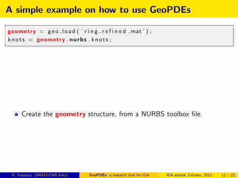
geometry = geo l o ad ( ’ r i n g r e f i n e d . mat ’ ) ;
knot s = geometry . nurbs . kno t s ;
Create the geometry structure, from a NURBS toolbox file.
Create the mesh structure in the parametric domain.
Map the mesh structure to the physical domain, using geometry.
Construct the space structure (the knots are stored in geometry).
Build the matrix and right-hand side.
R. Vazquez (IMATI-CNR Italy) GeoPDEs: a research tool for IGA IGA school, Cetraro, 2012 11 / 22
A simple example on how to use GeoPDEs
geometry = geo l o ad ( ’ r i n g r e f i n e d . mat ’ ) ;
knot s = geometry . nurbs . kno t s ;
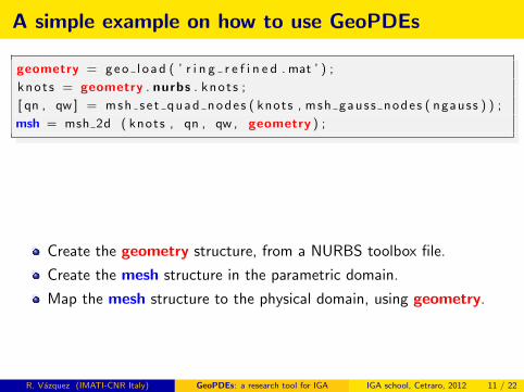
[ qn , qw ] = msh se t quad nodes ( knots , msh gauss nodes ( ngauss ) ) ;
msh = msh 2d ( knots , qn , qw , geometry ) ;
Create the geometry structure, from a NURBS toolbox file.
Create the mesh structure in the parametric domain.
Map the mesh structure to the physical domain, using geometry.
Construct the space structure (the knots are stored in geometry).
Build the matrix and right-hand side.
R. Vazquez (IMATI-CNR Italy) GeoPDEs: a research tool for IGA IGA school, Cetraro, 2012 11 / 22
A simple example on how to use GeoPDEs
geometry = geo l o ad ( ’ r i n g r e f i n e d . mat ’ ) ;
knot s = geometry . nurbs . kno t s ;
[ qn , qw ] = msh se t quad nodes ( knots , msh gauss nodes ( ngauss ) ) ;
msh = msh 2d ( knots , qn , qw , geometry ) ;
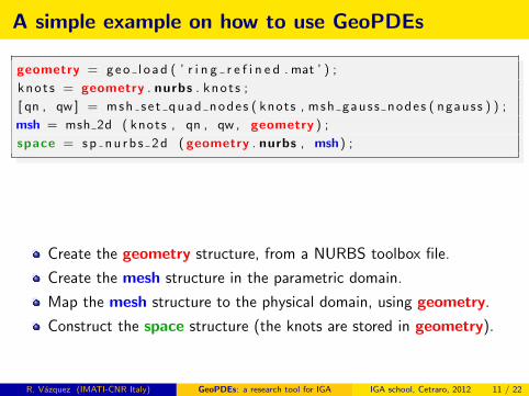
space = sp nu rb s 2d ( geometry . nurbs , msh) ;
Create the geometry structure, from a NURBS toolbox file.
Create the mesh structure in the parametric domain.
Map the mesh structure to the physical domain, using geometry.
Construct the space structure (the knots are stored in geometry).
Build the matrix and right-hand side.
R. Vazquez (IMATI-CNR Italy) GeoPDEs: a research tool for IGA IGA school, Cetraro, 2012 11 / 22
A simple example on how to use GeoPDEs
geometry = geo l o ad ( ’ r i n g r e f i n e d . mat ’ ) ;
knot s = geometry . nurbs . kno t s ;
[ qn , qw ] = msh se t quad nodes ( knots , msh gauss nodes ( ngauss ) ) ;
msh = msh 2d ( knots , qn , qw , geometry ) ;
space = sp nu rb s 2d ( geometry . nurbs , msh) ;
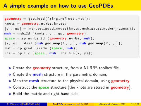
[ x , y ] = dea l (msh . geo map ( 1 , : , : ) , msh . geo map ( 2 , : , : ) ) ;
mat = op g radu g radv ( space , msh) ;
r h s = op f v ( space , msh , r h s f u n ( x , y ) ) ;
Create the geometry structure, from a NURBS toolbox file.
Create the mesh structure in the parametric domain.
Map the mesh structure to the physical domain, using geometry.
Construct the space structure (the knots are stored in geometry).
Build the matrix and right-hand side.
R. Vazquez (IMATI-CNR Italy) GeoPDEs: a research tool for IGA IGA school, Cetraro, 2012 11 / 22
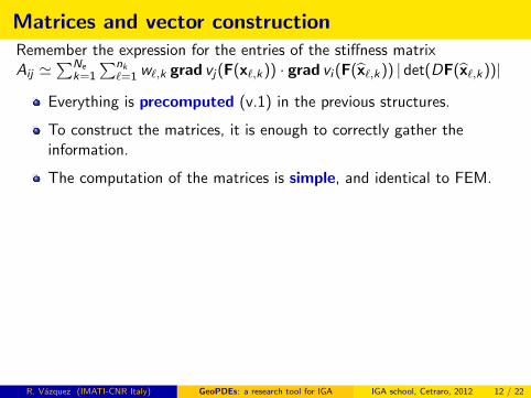
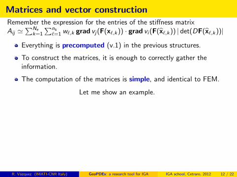
Matrices and vector constructionRemember the expression for the entries of the stiffness matrixAij '
∑Nek=1
∑nk`=1 w`,k grad vj(F(x`,k)) · grad vi (F(x`,k)) | det(DF(x`,k))|
Everything is precomputed (v.1) in the previous structures.
To construct the matrices, it is enough to correctly gather theinformation.
The computation of the matrices is simple, and identical to FEM.
Let me show an example.
f u n c t i o n mat = op g radu g radv ( space , msh)
f o r i e l = 1 :msh . n e l
mat loc = zeros ( space . nsh ( i e l ) , space . nsh ( i e l ) ) ;
f o r i d o f = 1 : space . nsh ( i e l )
i s h p = space . s h a p e f u n c t i o n g r a d i e n t s ( : , : , i d o f , i e l ) ;
f o r j d o f = 1 : space . nsh ( i e l )
j s h p = space . s h a p e f u n c t i o n g r a d i e n t s ( : , : , j d o f , i e l ) ;
f o r i node = 1 :msh . nqn
mat loc ( i d o f , j d o f ) += i s h p ( : , i node ) .∗ j s h p ( : , i node ) ∗msh . j a c d e t ( inode , i e l ) ∗ msh . quad weights ( inode , i e l ) ;
endfor %inode
endfor %j d o f
endfor %i d o f
mat ( space . connect ( : , i e l ) , space . connect ( : , i e l ) ) += mat loc ;
endfor %i e l
R. Vazquez (IMATI-CNR Italy) GeoPDEs: a research tool for IGA IGA school, Cetraro, 2012 12 / 22
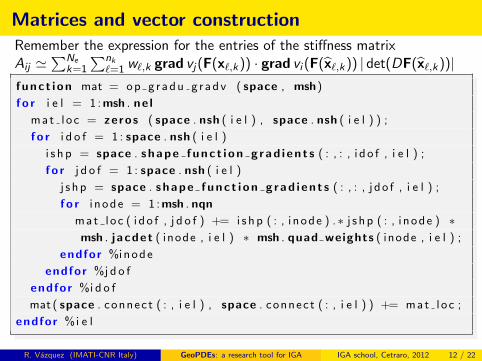
Matrices and vector constructionRemember the expression for the entries of the stiffness matrixAij '
∑Nek=1
∑nk`=1 w`,k grad vj(F(x`,k)) · grad vi (F(x`,k)) | det(DF(x`,k))|
f u n c t i o n mat = op g radu g radv ( space , msh)
f o r i e l = 1 :msh . n e l
mat loc = zeros ( space . nsh ( i e l ) , space . nsh ( i e l ) ) ;
f o r i d o f = 1 : space . nsh ( i e l )
i s h p = space . s h a p e f u n c t i o n g r a d i e n t s ( : , : , i d o f , i e l ) ;
f o r j d o f = 1 : space . nsh ( i e l )
j s h p = space . s h a p e f u n c t i o n g r a d i e n t s ( : , : , j d o f , i e l ) ;
f o r i node = 1 :msh . nqn
mat loc ( i d o f , j d o f ) += i s h p ( : , i node ) .∗ j s h p ( : , i node ) ∗msh . j a c d e t ( inode , i e l ) ∗ msh . quad weights ( inode , i e l ) ;
endfor %inode
endfor %j d o f
endfor %i d o f
mat ( space . connect ( : , i e l ) , space . connect ( : , i e l ) ) += mat loc ;
endfor %i e l
R. Vazquez (IMATI-CNR Italy) GeoPDEs: a research tool for IGA IGA school, Cetraro, 2012 12 / 22
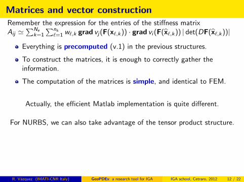
Matrices and vector constructionRemember the expression for the entries of the stiffness matrixAij '
∑Nek=1
∑nk`=1 w`,k grad vj(F(x`,k)) · grad vi (F(x`,k)) | det(DF(x`,k))|
Everything is precomputed (v.1) in the previous structures.
To construct the matrices, it is enough to correctly gather theinformation.
The computation of the matrices is simple, and identical to FEM.
Let me show an example.
Actually, the efficient Matlab implementation is quite different.
For NURBS, we can also take advantage of the tensor product structure.
f u n c t i o n mat = op g radu g radv ( space , msh)
f o r i e l = 1 :msh . n e l
mat loc = zeros ( space . nsh ( i e l ) , space . nsh ( i e l ) ) ;
f o r i d o f = 1 : space . nsh ( i e l )
i s h p = space . s h a p e f u n c t i o n g r a d i e n t s ( : , : , i d o f , i e l ) ;
f o r j d o f = 1 : space . nsh ( i e l )
j s h p = space . s h a p e f u n c t i o n g r a d i e n t s ( : , : , j d o f , i e l ) ;
f o r i node = 1 :msh . nqn
mat loc ( i d o f , j d o f ) += i s h p ( : , i node ) .∗ j s h p ( : , i node ) ∗msh . j a c d e t ( inode , i e l ) ∗ msh . quad weights ( inode , i e l ) ;
endfor %inode
endfor %j d o f
endfor %i d o f
mat ( space . connect ( : , i e l ) , space . connect ( : , i e l ) ) += mat loc ;
endfor %i e l
R. Vazquez (IMATI-CNR Italy) GeoPDEs: a research tool for IGA IGA school, Cetraro, 2012 12 / 22
Boundary conditions: the boundary substructures
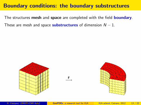
The structures mesh and space are completed with the field boundary.
These are mesh and space substructures of dimension N − 1.
The boundary structures have some particularities:
jacdet contains the area element of the boundary parameterization.
The space structure uses a local numbering for each boundary.
A new field, dofs, is added to recover the global numbering.
F−→
R. Vazquez (IMATI-CNR Italy) GeoPDEs: a research tool for IGA IGA school, Cetraro, 2012 13 / 22
Boundary conditions: the boundary substructures
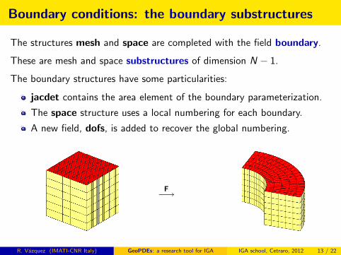
The structures mesh and space are completed with the field boundary.
These are mesh and space substructures of dimension N − 1.
The boundary structures have some particularities:
jacdet contains the area element of the boundary parameterization.
The space structure uses a local numbering for each boundary.
A new field, dofs, is added to recover the global numbering.
F−→
R. Vazquez (IMATI-CNR Italy) GeoPDEs: a research tool for IGA IGA school, Cetraro, 2012 13 / 22

Boundary conditions: the boundary substructures
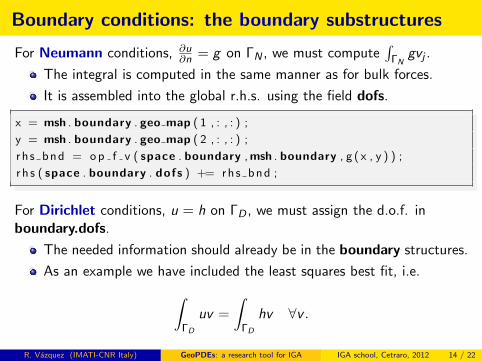
For Neumann conditions, ∂u∂n = g on ΓN , we must compute
∫ΓN
gvj .
The integral is computed in the same manner as for bulk forces.
It is assembled into the global r.h.s. using the field dofs.
x = msh . boundary . geo map ( 1 , : , : ) ;
y = msh . boundary . geo map ( 2 , : , : ) ;
r h s bnd = op f v ( space . boundary , msh . boundary , g ( x , y ) ) ;
r h s ( space . boundary . dofs ) += rhs bnd ;
For Dirichlet conditions, u = h on ΓD , we must assign the d.o.f. inboundary.dofs.
The needed information should already be in the boundary structures.
As an example we have included the least squares best fit, i.e.∫ΓD
uv =
∫ΓD
hv ∀v .
R. Vazquez (IMATI-CNR Italy) GeoPDEs: a research tool for IGA IGA school, Cetraro, 2012 14 / 22
Boundary conditions: the boundary substructures
For Neumann conditions, ∂u∂n = g on ΓN , we must compute
∫ΓN
gvj .
The integral is computed in the same manner as for bulk forces.
It is assembled into the global r.h.s. using the field dofs.
x = msh . boundary . geo map ( 1 , : , : ) ;
y = msh . boundary . geo map ( 2 , : , : ) ;
r h s bnd = op f v ( space . boundary , msh . boundary , g ( x , y ) ) ;
r h s ( space . boundary . dofs ) += rhs bnd ;
For Dirichlet conditions, u = h on ΓD , we must assign the d.o.f. inboundary.dofs.
The needed information should already be in the boundary structures.
As an example we have included the least squares best fit, i.e.∫ΓD
uv =
∫ΓD
hv ∀v .
R. Vazquez (IMATI-CNR Italy) GeoPDEs: a research tool for IGA IGA school, Cetraro, 2012 14 / 22
A simple example on how to use GeoPDEs
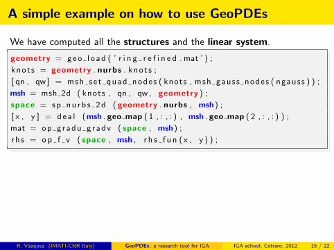
We have computed all the structures and the linear system.
geometry = geo l o ad ( ’ r i n g r e f i n e d . mat ’ ) ;
knot s = geometry . nurbs . kno t s ;
[ qn , qw ] = msh se t quad nodes ( knots , msh gauss nodes ( ngauss ) ) ;
msh = msh 2d ( knots , qn , qw , geometry ) ;
space = sp nu rb s 2d ( geometry . nurbs , msh) ;
[ x , y ] = dea l (msh . geo map ( 1 , : , : ) , msh . geo map ( 2 , : , : ) ) ;
mat = op g radu g radv ( space , msh) ;
r h s = op f v ( space , msh , r h s f u n ( x , y ) ) ;
R. Vazquez (IMATI-CNR Italy) GeoPDEs: a research tool for IGA IGA school, Cetraro, 2012 15 / 22
A simple example on how to use GeoPDEs
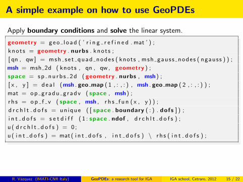
Apply boundary conditions and solve the linear system.
geometry = geo l o ad ( ’ r i n g r e f i n e d . mat ’ ) ;
knot s = geometry . nurbs . kno t s ;
[ qn , qw ] = msh se t quad nodes ( knots , msh gauss nodes ( ngauss ) ) ;
msh = msh 2d ( knots , qn , qw , geometry ) ;
space = sp nu rb s 2d ( geometry . nurbs , msh) ;
[ x , y ] = dea l (msh . geo map ( 1 , : , : ) , msh . geo map ( 2 , : , : ) ) ;
mat = op g radu g radv ( space , msh) ;
r h s = op f v ( space , msh , r h s f u n ( x , y ) ) ;
d r c h l t d o f s = un ique ( [ space . boundary ( : ) . dofs ] ) ;
i n t d o f s = s e t d i f f ( 1 : space . ndof , d r c h l t d o f s ) ;
u ( d r c h l t d o f s ) = 0 ;
u ( i n t d o f s ) = mat ( i n t d o f s , i n t d o f s ) \ r h s ( i n t d o f s ) ;
R. Vazquez (IMATI-CNR Italy) GeoPDEs: a research tool for IGA IGA school, Cetraro, 2012 15 / 22
A simple example on how to use GeoPDEs
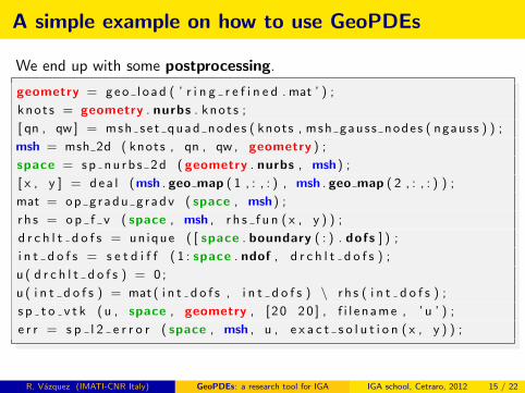
We end up with some postprocessing.
geometry = geo l o ad ( ’ r i n g r e f i n e d . mat ’ ) ;
knot s = geometry . nurbs . kno t s ;
[ qn , qw ] = msh se t quad nodes ( knots , msh gauss nodes ( ngauss ) ) ;
msh = msh 2d ( knots , qn , qw , geometry ) ;
space = sp nu rb s 2d ( geometry . nurbs , msh) ;
[ x , y ] = dea l (msh . geo map ( 1 , : , : ) , msh . geo map ( 2 , : , : ) ) ;
mat = op g radu g radv ( space , msh) ;
r h s = op f v ( space , msh , r h s f u n ( x , y ) ) ;
d r c h l t d o f s = un ique ( [ space . boundary ( : ) . dofs ] ) ;
i n t d o f s = s e t d i f f ( 1 : space . ndof , d r c h l t d o f s ) ;
u ( d r c h l t d o f s ) = 0 ;
u ( i n t d o f s ) = mat ( i n t d o f s , i n t d o f s ) \ r h s ( i n t d o f s ) ;
s p t o v t k (u , space , geometry , [ 20 20 ] , f i l e name , ’ u ’ ) ;
e r r = s p l 2 e r r o r ( space , msh , u , e x a c t s o l u t i o n ( x , y ) ) ;
R. Vazquez (IMATI-CNR Italy) GeoPDEs: a research tool for IGA IGA school, Cetraro, 2012 15 / 22
A simple example on how to use GeoPDEs
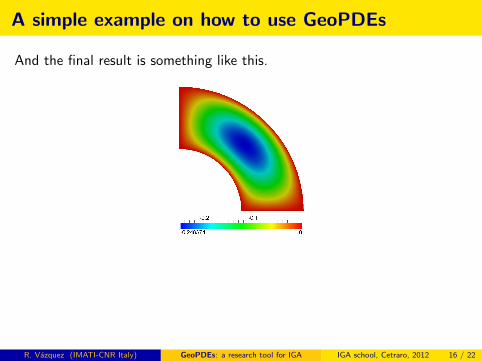
And the final result is something like this.
The package contains several simple examples:
h-,p-,k-refinement, 2D and 3D, B-splines and NURBS...
The structures can be easily extended to solve more complex problems.
R. Vazquez (IMATI-CNR Italy) GeoPDEs: a research tool for IGA IGA school, Cetraro, 2012 16 / 22
A simple example on how to use GeoPDEs
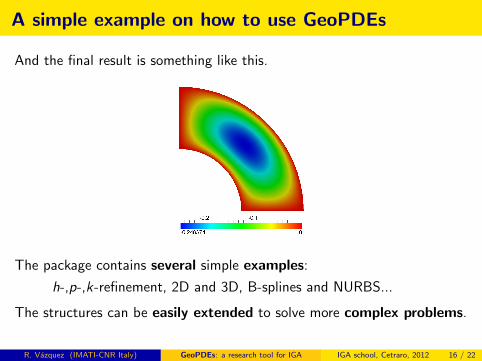
And the final result is something like this.
The package contains several simple examples:
h-,p-,k-refinement, 2D and 3D, B-splines and NURBS...
The structures can be easily extended to solve more complex problems.
R. Vazquez (IMATI-CNR Italy) GeoPDEs: a research tool for IGA IGA school, Cetraro, 2012 16 / 22
Linear elasticity problems: the elasticity package
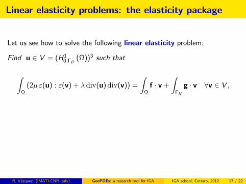
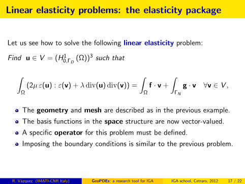
Let us see how to solve the following linear elasticity problem:
Find u ∈ V = (H10,ΓD
(Ω))3 such that
∫Ω
(2µ ε(u) : ε(v) + λdiv(u) div(v)) =
∫Ω
f · v +
∫ΓN
g · v ∀v ∈ V ,
The geometry and mesh are described as in the previous example.
The basis functions in the space structure are now vector-valued.
A specific operator for this problem must be defined.
Imposing the boundary conditions is similar to the previous problem.
R. Vazquez (IMATI-CNR Italy) GeoPDEs: a research tool for IGA IGA school, Cetraro, 2012 17 / 22
Linear elasticity problems: the elasticity package
Let us see how to solve the following linear elasticity problem:
Find u ∈ V = (H10,ΓD
(Ω))3 such that
∫Ω
(2µ ε(u) : ε(v) + λdiv(u) div(v)) =
∫Ω
f · v +
∫ΓN
g · v ∀v ∈ V ,
The geometry and mesh are described as in the previous example.
The basis functions in the space structure are now vector-valued.
A specific operator for this problem must be defined.
Imposing the boundary conditions is similar to the previous problem.
R. Vazquez (IMATI-CNR Italy) GeoPDEs: a research tool for IGA IGA school, Cetraro, 2012 17 / 22
Definition of the vectorial space
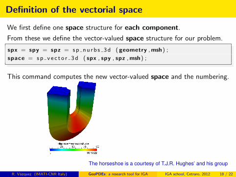
We first define one space structure for each component.
From these we define the vector-valued space structure for our problem.
spx = spy = spz = sp nu rb s 3d ( geometry , msh) ;
space = sp v e c t o r 3 d ( spx , spy , spz , msh) ;
This command computes the new vector-valued space and the numbering.
The horseshoe is a courtesy of T.J.R. Hughes’ and his group
R. Vazquez (IMATI-CNR Italy) GeoPDEs: a research tool for IGA IGA school, Cetraro, 2012 18 / 22
Definition of the vectorial space
We first define one space structure for each component.
From these we define the vector-valued space structure for our problem.
spx = spy = spz = sp nu rb s 3d ( geometry , msh) ;
space = sp v e c t o r 3 d ( spx , spy , spz , msh) ;
This command computes the new vector-valued space and the numbering.
The horseshoe is a courtesy of T.J.R. Hughes’ and his group
R. Vazquez (IMATI-CNR Italy) GeoPDEs: a research tool for IGA IGA school, Cetraro, 2012 18 / 22
Electromagnetism: the Maxwell package
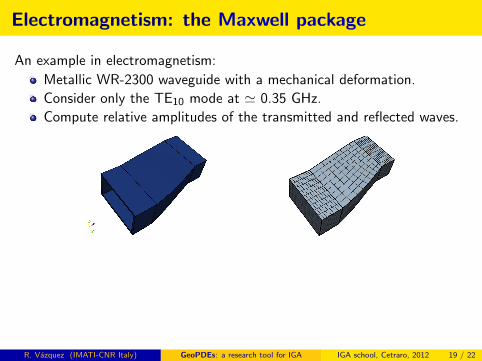
An example in electromagnetism:
Metallic WR-2300 waveguide with a mechanical deformation.
Consider only the TE10 mode at ' 0.35 GHz.
Compute relative amplitudes of the transmitted and reflected waves.
Time-harmonic Maxwell equations in the interior of the waveguide.
Forward (known) and reverse (unknown) traveling waves at Γi .
Forward (unknown) traveling wave at Γo .
Perfect electrical conductor (E× n = 0) on the other boundaries.
R. Vazquez (IMATI-CNR Italy) GeoPDEs: a research tool for IGA IGA school, Cetraro, 2012 19 / 22
Electromagnetism: the Maxwell package
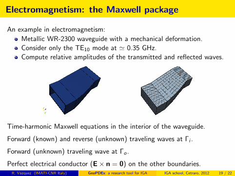
An example in electromagnetism:
Metallic WR-2300 waveguide with a mechanical deformation.
Consider only the TE10 mode at ' 0.35 GHz.
Compute relative amplitudes of the transmitted and reflected waves.
Time-harmonic Maxwell equations in the interior of the waveguide.
Forward (known) and reverse (unknown) traveling waves at Γi .
Forward (unknown) traveling wave at Γo .
Perfect electrical conductor (E× n = 0) on the other boundaries.R. Vazquez (IMATI-CNR Italy) GeoPDEs: a research tool for IGA IGA school, Cetraro, 2012 19 / 22
Electromagnetism: the Maxwell package
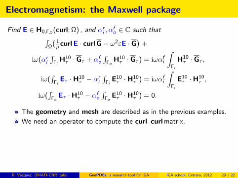
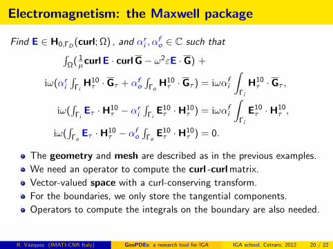
Find E ∈ H0,ΓD(curl; Ω) , and αr
i , αfo ∈ C such that∫
Ω( 1µcurl E · curl G− ω2εE · G) +
iω(αri
∫Γi
H10τ · Gτ + αf
o
∫Γo
H10τ · Gτ ) = iωαf
i
∫Γi
H10τ · Gτ ,
iω(∫
ΓiEτ ·H10
τ − αri
∫Γi
E10τ ·H10
τ ) = iωαfi
∫Γi
E10τ ·H10
τ ,
iω(∫
ΓoEτ ·H10
τ − αfo
∫Γo
E10τ ·H10
τ ) = 0.
The geometry and mesh are described as in the previous examples.
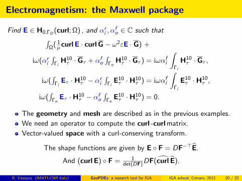
We need an operator to compute the curl -curl matrix.
Vector-valued space with a curl-conserving transform.
The shape functions are given by E F = DF−>E.
And (curl E) F = 1det(DF)DF(curl E).
R. Vazquez (IMATI-CNR Italy) GeoPDEs: a research tool for IGA IGA school, Cetraro, 2012 20 / 22
Electromagnetism: the Maxwell package
Find E ∈ H0,ΓD(curl; Ω) , and αr
i , αfo ∈ C such that∫
Ω( 1µcurl E · curl G− ω2εE · G) +
iω(αri
∫Γi
H10τ · Gτ + αf
o
∫Γo
H10τ · Gτ ) = iωαf
i
∫Γi
H10τ · Gτ ,
iω(∫
ΓiEτ ·H10
τ − αri
∫Γi
E10τ ·H10
τ ) = iωαfi
∫Γi
E10τ ·H10
τ ,
iω(∫
ΓoEτ ·H10
τ − αfo
∫Γo
E10τ ·H10
τ ) = 0.
The geometry and mesh are described as in the previous examples.
We need an operator to compute the curl -curl matrix.
Vector-valued space with a curl-conserving transform.
For the boundaries, we only store the tangential components.
Operators to compute the integrals on the boundary are also needed.
R. Vazquez (IMATI-CNR Italy) GeoPDEs: a research tool for IGA IGA school, Cetraro, 2012 20 / 22
Electromagnetism: the Maxwell package
Find E ∈ H0,ΓD(curl; Ω) , and αr
i , αfo ∈ C such that∫
Ω( 1µcurl E · curl G− ω2εE · G) +
iω(αri
∫Γi
H10τ · Gτ + αf
o
∫Γo
H10τ · Gτ ) = iωαf
i
∫Γi
H10τ · Gτ ,
iω(∫
ΓiEτ ·H10
τ − αri
∫Γi
E10τ ·H10
τ ) = iωαfi
∫Γi
E10τ ·H10
τ ,
iω(∫
ΓoEτ ·H10
τ − αfo
∫Γo
E10τ ·H10
τ ) = 0.
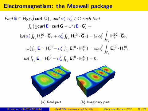
(a) Real part (b) Imaginary part
R. Vazquez (IMATI-CNR Italy) GeoPDEs: a research tool for IGA IGA school, Cetraro, 2012 20 / 22
GeoPDEs 2.0
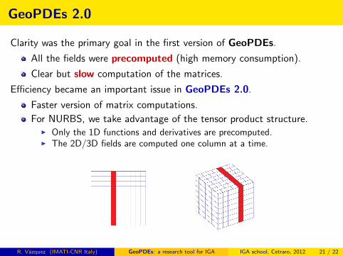
Clarity was the primary goal in the first version of GeoPDEs.
All the fields were precomputed (high memory consumption).
Clear but slow computation of the matrices.
Efficiency became an important issue in GeoPDEs 2.0.
Faster version of matrix computations.
For NURBS, we take advantage of the tensor product structure.I Only the 1D functions and derivatives are precomputed.I The 2D/3D fields are computed one column at a time.
R. Vazquez (IMATI-CNR Italy) GeoPDEs: a research tool for IGA IGA school, Cetraro, 2012 21 / 22
GeoPDEs 2.0
Clarity was the primary goal in the first version of GeoPDEs.
All the fields were precomputed (high memory consumption).
Clear but slow computation of the matrices.
Efficiency became an important issue in GeoPDEs 2.0.
Faster version of matrix computations.I Vectorization of some loops.I Better use of sparse matrices in Matlab.
For NURBS, we take advantage of the tensor product structure.I Only the 1D functions and derivatives are precomputed.I The 2D/3D fields are computed one column at a time.
R. Vazquez (IMATI-CNR Italy) GeoPDEs: a research tool for IGA IGA school, Cetraro, 2012 21 / 22
GeoPDEs 2.0
Clarity was the primary goal in the first version of GeoPDEs.
All the fields were precomputed (high memory consumption).
Clear but slow computation of the matrices.
Efficiency became an important issue in GeoPDEs 2.0.
Faster version of matrix computations.
For NURBS, we take advantage of the tensor product structure.I Only the 1D functions and derivatives are precomputed.I The 2D/3D fields are computed one column at a time.
R. Vazquez (IMATI-CNR Italy) GeoPDEs: a research tool for IGA IGA school, Cetraro, 2012 21 / 22
GeoPDEs 2.0
Clarity was the primary goal in the first version of GeoPDEs.
All the fields were precomputed (high memory consumption).
Clear but slow computation of the matrices.
Efficiency became an important issue in GeoPDEs 2.0.
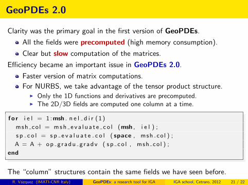
Faster version of matrix computations.
For NURBS, we take advantage of the tensor product structure.I Only the 1D functions and derivatives are precomputed.I The 2D/3D fields are computed one column at a time.
f o r i e l = 1 :msh . n e l d i r ( 1 )
msh co l = msh e v a l u a t e c o l (msh , i e l ) ;
s p c o l = s p e v a l u a t e c o l ( space , msh co l ) ;
A = A + op g radu g radv ( s p c o l , msh co l ) ;
end
The “column” structures contain the same fields we have seen before.R. Vazquez (IMATI-CNR Italy) GeoPDEs: a research tool for IGA IGA school, Cetraro, 2012 21 / 22
Conclusions
GeoPDEs is an open source and free Matlab implementation of IGA.
Very useful for teaching purposes and for new researchers.
It can serve as a rapid prototyping tool to test new ideas.
Several packages already released to solve different problems.
Many examples and a short guide with detailed explanations.
In the last 4 months, around 300 downloads of the base package.
Contributions are welcome, to improve the code or to show new methods.
GeoPDEs tutorial today at 17:00.
Software download and information
http://geopdes.sourceforge.net
Thanks for your attention!
R. Vazquez (IMATI-CNR Italy) GeoPDEs: a research tool for IGA IGA school, Cetraro, 2012 22 / 22