Geometry of State Spaces - uni-leipzig.deuhlmann/PDF/UC07.pdf · Geometry of State Spaces 5 1.2 Length of curves in H We ask for the length of a curve in Hilbert space. The curve

Geometry of State Spaces

Armin Uhlmann and Bernd Crell

Institut fur Theoretische Physik, Universitat [email protected]

[email protected]

In the Hilbert space description of quantum theory one has two major inputs:Firstly its linearity, expressing the superposition principle, and, secondly, thescalar product, allowing to compute transition probabilities. The scalar prod-uct defines an Euclidean geometry. One may ask for the physical meaningin quantum physics of geometric constructs in this setting. As an importantexample we consider the length of a curve in Hilbert space and the “velocity”,i. e. the length of the tangents, with which the vector runs through the Hilbertspace.

The Hilbert spaces are generically complex in quantum physics: There isa multiplication with complex numbers: Two linear dependent vectors rep-resent the same state. By restricting to unit vectors one can diminish thisarbitrariness to phase factors.

As a consequence, two curves of unit vectors represent the same curveof states if they differ only in phase. They are physically equivalent. Thus,considering a given curve — for instance a piece of a solution of a Schrodingerequation – one can ask for an equivalent curve of minimal length. This minimallength is the “Fubini-Study length”. The geometry, induced by the minimallength requirement in the set of vector states, is the “Fubini-Study metric”.

There is a simple condition from which one can read off whether all piecesof a curve in Hilbert space fulfill the minimal length condition, so that theirEuclidean and their Study-Fubini length coincide piecewise: It is the paralleltransport condition, defining the geometric (or Berry) phase of closed curvesby the following mechanism: We replace the closed curve by changing itsphases to a minimal length curve. Generically, the latter will not close. Itsinitial and its final point will differ by a phase factor, called the geometricphase (factor). We only touch these aspects in our essay and advice the readingof [6] instead. We discuss, as quite another application, the Tam-Mandelstamminequalities.

The set of vector states associated to a Hilbert space can also be describedas the set of its 1-dimensional subspaces or, equivalently, as the set of all rankone projection operators. Geometrically it is the “projective space” given by

2 Armin Uhlmann and Bernd Crell

the Hilbert space in question. In finite dimension it is a well studied manifold1.Again, we advice the reader to a more comprehensive monograph, say [23],to become acquainted with projective spaces in quantum theory. We justlike to point to one aspect: Projective spaces are rigid. A map, transformingour projective space one–to–one onto itself and preserving its Fubini-Studydistances, is a Wigner symmetry. On the the Hilbert space level this is atheorem of Wigner asserting that such a map can be induced by a unitary orby an anti-unitary transformation.

After these lengthy introduction to our first chapter, we have not muchto comment to our third one. It is just devoted to the (partial) extension ofwhat has been said above to general state spaces. It will be done mainly, butnot only, by purification methods.

The central objects are the generalized transition probability (“fidelity”),the Bures distance, and its Riemann metric. These concepts can be defined,and show similar features, in all quantum state spaces. They are “universal”in quantum physics.

However, at the beginning of quantum theory people were not sure whetherdensity operators describe states of a quantum system or not. In our days, wethink, the question is completely settled. There are genuine quantum statesdescribed by density operators. But not only that, the affirmative answeropened new insight into the basic structure of quantum theory. The secondchapter is dedicated to these structural questions.

To a Hilbert spaces H one associates the algebra B(H) of all boundedoperators which mapH into itself. With a density operator ω and any operatorA ∈ B(H), the number

ω(A) = trAω

is the expectation value of A, provided the “system is in the state given by ω“.Now ω is linear in A, it attains positive values or zero for positive operators,and it returns 1 if we compute the expectation value of the identity operator1. These properties are subsumed by saying “ω is a normalized positive linearfunctional on the algebra B(H)”. Exactly such functionals are also called“states of B(H) ”, asserting that every one of these objects can possibly be astate of our quantum system.

If the Hilbert space is of finite dimension then every state of B(H) can becharacterized by a density operator. But in the other, infinite cases, there arein addition states of quite different nature, the so-called singular ones. Theycan be ignored in theories with finitely many degrees of freedom, for instancein Schrodinger theory. But in treating unbounded many degrees of freedomwe have to live with them.

One goes an essential step further in considering more general algebrasthan B(H). The idea is that a quantum system is defined, ignoring other

1 It is certainly the most important algebraic variety.

Geometry of State Spaces 3

demands, by its observables. States should be identified by their expectationvalues. However, not any set of observables should be considered as a quantumsystem. There should be an algebra, say A, associated to a quantum systemcontaining the relevant observables. Besides being an algebra (over the com-plex numbers), an Hermitian adjoint, A† should be defined for every A ∈ Aand, finally, there should be “enough” states of A.

As a matter of fact, these requirement are sufficient if A is of finite di-mension as a linear space. Then the algebra can be embedded as a so-called∗-subalgebra in any algebra B(H) with dimH sufficient large or infinite. Re-lying on Wedderburn’s theorem, we describe all these algebras and their statespaces, They all can be gained by performing direct products and direct sumsof some algebras B(H). Intrinsically they are enumerated by their “type”, afinite set of positive numbers. We abbreviate this set by d to shorten the moreprecise notation Id for so-called type one algebras.

If the algebras are not finite, things are much more involved. There are vonNeumann (i. e. concrete W∗-) algebras, C∗-algebras, and more general classesof algebras. About them we say (almost) nothing but refer, for a physicalmotivated introduction, to [10].

Let us stress, however, a further point of view. In a bipartite system, whichis the direct product of two other ones, ( – say Alice’s and Bob’s – ), bothsystems are embedded in the larger one as subsystems. Their algebras becomesubalgebras of another, larger algebra.

There is a more general point of view: It is a good idea to imagine the quan-tum world as a hierarchy of quantum systems. An “algebra of observables”is attached to each one, together with its state space. The way, an algebrais a subalgebra of another one, is describing how the former one should beunderstood as a quantum subsystem of a “larger” one.

Let us imagine such a hierarchical structure. A state in one of these systemsdetermines a state in every of its subsystems: We just have to look at the stateby using the operators of the subsystem in question only, i. e. we recognizewhat possibly can be observed by the subsystems observables.

Restricting a state of a quantum system (of an algebra) to a subsystem(to a subalgebra) is equivalent to the “partial trace” in direct products. Itextends the notion to more general settings.

On the other hand, starting with a system, every operator remains anoperator in all larger systems containing the original one as a subsystem. Toa large amount the physical meaning of a quantum system, its operators andits states, is determined by its relations to other quantum systems.

There is an appendix devoted to the geometric mean, the perhaps mostimportant operator mean. It provides a method to handle two positive op-erators in general position. Only one subsection of the appendix is directlyconnected with the third chapter: How parallel lifts of Alice’s states are seenby Bob.


As a matter of fact, a chapter describing more subtle problems of convex-ity had been proposed. But we could not finish it in due time. Most of theappendix has been prepared for it. Nevertheless, in the main part there isa short description of the convex structure of states spaces in finite systems(faces, extremal points, rigidity).

1 Geometry of pure states

1.1 Norm and distance in Hilbert space

Let us consider a Hilbert space2 H. Its elements are called vectors. If notexplicitly stated otherwise, we consider complex Hilbert spaces, i. e. the mul-tiplication of vectors with complex numbers is allowed. Vectors will be denotedeither by their mathematical notation, say ψ, or by Dirac’s, say |ψ〉.

For the scalar product we write accordingly3

〈ϕ,ψ〉 or 〈ϕ|ψ〉 .

The norm or vector norm of ψ ∈ H reads

‖ ψ ‖ :=√〈ψ, ψ〉 = vector norm of ψ .

It is the Euclidian length of the vector ψ. One defines

‖ ψ − ψ′ ‖ = distance between ψ and ψ′

which is an Euclidean distance: If in any basis, |j〉, j = 1, 2, . . ., one gets

|ψ〉 =∑

zj |j〉, zj = xj + iyj ,

and, with coefficients z′j , the similar expansion for ψ′, then

‖ ψ − ψ′ ‖= (∑

[xj − x′j ]2 + [yj − y′j ]

2)1/2 ,

and this justifies the name “Euclidean distance”.The scalar product defines the norm and the norm the Euclidean geometry

of H. In turn one can obtain the scalar product from the vector norm:

4〈ψ, ψ′〉 =‖ ψ + ψ′ ‖2 − ‖ ψ − ψ′ ‖2 −i ‖ ψ + iψ′ ‖2 +i ‖ ψ − iψ′ ‖2

The scalar product allows for the calculation of quantum probabilities. Nowwe see that, due to the complex structure of H, these probabilities are alsoencoded in its Euclidean geometry.2 We only consider Hilbert spaces with countable bases.3 We use the ”physicist’s convention” that the scalar product is anti-linear in ϕ

and linear in ψ.


1.2 Length of curves in HWe ask for the length of a curve in Hilbert space. The curve may be given by

t → ψt, 0 ≤ t ≤ 1 (1)

where t is a parameter, not necessarily the time. We assume that for all ϕ ∈ Hthe function t → 〈ϕ,ψt〉 of t is continuous.

To get the length of (1) we have to take all subdivisions

0 ≤ t0 < t1 < . . . < tn ≤ 1

in performing the sup,

length of the curve = supn∑

j=1

‖ ψtj−1 − ψtj‖ . (2)

The length is independent of the parameter choice.If we can guaranty the existence of

ψt =d

dtψt ∈ H (3)

then one knows

length of the curve =∫ 1

0

√〈ψt, ψt〉 dt . (4)

The vector ψt is the (contra-variant) tangent along (1). Its lengths is thevelocity with which4 ψ = ψt travels through H, i. e.

ds

dt=

√〈ψ, ψ〉 . (5)

Interesting examples are solutions t → ψt of a Schrodinger equation,

Hψ = ihψ . (6)

In this case the tangent vector is time independent and we get

ds

dt= h−1

√〈ψ, H2ψ〉 . (7)

The length of the solution between the times t0 and t1 is

length = h−1(t1 − t0)√〈ψ, H2ψ〉 (8)

Anandan,[28], has put forward the idea to consider the Euclidean length (5) asan intrinsic and universal parameter in Hilbert space. For example, consider4 We often write just ψ instead of ψt.


dt

ds= 〈ψ, ψ〉−1/2 = h (〈ψ, H2ψ〉)−1/2

instead of ds/dt and interpret it as the quantum velocity with which time iselapsing during a Schrodinger evolution. Also other metrical structures, towhich we come later on, allow for similar interpretations.Remark: Though we shall be interested mostly in finite dimensional Hilbertspaces or, in the infinite case, in bounded operators, let us have a short lookat the general case.

In the Schrodinger theory H, the Hamilton operator, is usually “un-bounded” and there are vectors not in the domain of definition of H. However,there is always an integrated version: A unitary group

t → U(t) = exp(tH

ih)

which can be defined rigorously for self-adjoint H.Then ψ0 belongs to the domain of definition of H exactly if the tangents (3)of the curve ψt = U(t)ψ0 exist. If the tangents exist then the Hamiltonian canbe gained by

ih limε→0

U(t + ε)− U(t)ε

ψ = Hψ

and (7) and (8) apply.If, however, ψ0 does not belong to the domain of definition of H, then (2)returns ∞ for the length of every piece of the curve t → U(t)ψ0. In this casethe vector runs, during a finite time interval, through an infinitely long pieceof t → ψt. The velocity ds/dt must be infinite.

1.3 Distance and length

Generally, a distance “dist” in a space attaches a real and not negative numberto any pair of points satisfyinga) dist(ξ1, ξ2) = dist(ξ2, ξ1)b) dist(ξ1, ξ2) + dist(ξ2, ξ3) ≥ dist(ξ1, ξ3),c) dist(ξ1, ξ2) = 0 ⇔ ξ1 = ξ2.A set with a distance is a metric space.

Given the distance, dist(., .), of a metric space and two different points, sayξ0 and ξ1, one may ask for the length of a continuous curve connecting thesetwo points5. The inf of the lengths over all these curves is again a distance,the inner distance. The inner distance, distinner(ξ0, ξ1) is never smaller thanthe original one,

distinner(ξ0, ξ1) ≥ dist(ξ0, ξ1)

If equality holds, the distance (and the metric space) is called inner. A curve,connecting ξ0 and ξ1, the length of which equals the distance between the5 We assume that for every pair of points such curves exist.


two point, is called a “short geodesic” arc. A curve, which is short geodesicbetween all sufficiently near points, is a geodesic.

The Euclidian distance is an inner distance. It is easy to present the short-est curves between to vectors, ψ1 and ψ0, in Hilbert space:

t → ψt = (1− t)ψ0 + tψ1, ψ = ψ1 − ψ0 . (9)

is a short geodesic arc between both vectors.In Euclidean spaces the shortest connection between two points is a piece

of a straight line, and this geodesic arc is unique. Indeed, from (9) we conclude

‖ ψt − ψr ‖= |t− r| ‖ ψ1 − ψ0 ‖ . (10)

With this relation we can immediately compute (2) and we see that the lengthof (9) is equal to the distance between starting and end point.We have seen something more general: If in a linear space the distance isdefined by a norm, the metric is inner and the geodesics are of the form (9).

1.4 Curves on the unit sphere

Restricting the geometry of H to the unit sphere ψ ∈ H, ‖ ψ ‖= 1 can becompared with the change from Euclidean geometry to spherical geometry inan Euclidean 3-space. In computing a length by (2) only curves on the sphereare allowed.

The geodesics on a unit sphere are great circles. These are sections ofthe sphere with a plane that contains the center of the sphere. The sphericaldistance of two points, say ψ0 and ψ1, is the angle, α, between the rays fromthe center of the sphere to the two points in question.

distspherical(ψ1, ψ0) = angle between the radii pointing to ψ0 and ψ1 (11)

with the restriction 0 ≤ α ≤ π of the angle α. By the additivity modulo 2π ofthe angle one can compute (2) along a great circle to see that (11) is an innermetric.

If the two points are not antipodes, ψ0 + ψ1 6= 0, then the great circlecrossing through them and short geodesic arc between the two vectors isunique.For antipodes the great circle crossing through them is not unique and thereare many short geodesic arcs of length π connecting them.

By elementary geometry

‖ ψ1 − ψ0 ‖=√

2− 2 cos α = 2 sinα

2(12)

and cos α can be computed by

cos α =〈ψ0, ψ1〉+ 〈ψ1, ψ0〉

2(13)


We see from (13) thatcos α ≤ |〈ψ0, ψ1〉| (14)

Therefore, we have the following statement:The length of a curve on the unit sphere connecting ψ0 with ψ1 is at least

arccos |〈ψ0, ψ1〉| .

Applying this observation to the solution of a Schrodinger equation onegets the Mandelstam-Tamm inequalities, [57]. To get them one simply com-bines (14) with (8): If a solution ψt of the Schrodinger equation (6) goes attime t = t0 through the unit vector ψ0 and at time t = t1 through ψ1, then

(t1 − t0)√〈ψ,H2ψ〉 ≥ h arccos |〈ψ0, ψ1〉| (15)

must be valid. (Remember that H is conserved along solutions of (6) and wecan use any ψ = ψt from the assumed solution.)However, a sharper inequality holds,

(t1 − t0)√〈ψ, H2ψ〉 − 〈ψ,Hψ〉2 ≥ h arccos |〈ψ0, ψ1〉| . (16)

Namely, the right-hand side is invariant against “gauge transformations”

ψt 7→ ψ′t = (exp iγt) ψt .

The left side of (16) does not change in substituting H by H ′ = H − γ1 andψ′t is a solution of

H ′ψ′ = ihψ′ .

Hence we can “gauge away” the extra term in (16) to get the inequality (15).

Remarks:a) The reader will certainly identify the square root expression in (16) asthe “uncertainty” 4ψ(H) of H in the state given by the unit vector ψ. Morespecific, (16) provides the strict lower bound T4ψ(H) ≥ h/4 for the time Tto convert ψ to a vector orthogonal to ψ by a Schrodinger evolution.b) If U(r) is a one-parameter unitary group with generator A, then

|r|4ψ(A) ≥ arccos |〈ψ, U(r)ψ〉|.

Interesting candidates are the position and the momentum operators, theangular momentum along an axis, occupation number operators, and so on.c) The tangent space consists of pairs ψ, ψ with a tangent or velocity vectorψ, reminiscent from a curve crossing through ψ. The fiber of all tangents basedat ψ carries the positive quadratic form

ψ1, ψ2 → 〈ψ, ψ〉〈ψ1, ψ2〉 − 〈ψ1, ψ〉〈ψ, ψ2〉


gained by polarization.d) More general than proposed in (16), one can say something about timedependent Hamiltonians, H(t), and the Schodinger equation

H(t)ψ = ihψ . (17)

If a solution of (17) is crossing the unit vectors ψj at times tj , then

∫ t1

t0

√〈ψ, H2ψ〉 − 〈ψ,Hψ〉2dt ≥ h arccos |〈ψ0, ψ1〉| . (18)

For further application to the speed of quantum evolutions see [43].

1.5 Phases

If the vectors ψ and ψ′ are linearly dependent, they describe the same state.

ψ 7→ πψ =|ψ〉〈ψ|〈ψ,ψ〉 (19)

maps the vectors of H onto the pure states, with the exception of the zerovector. Multiplying a vector by a complex number different from zero is thenatural gauge transformation offered by H.From this freedom in choosing a state vector for a pure state,

ψ → εψ, |ε| = 1, (20)

the phase change, is of primary physical interest.

In the following we consider parameterized curve as in (1) on the unitsphere of H. At first we see

〈ψt, ψt〉 is purely imaginary. (21)

To see this one differentiates

0 =d

dt〈ψ, ψ〉 = 〈ψ, ψ〉+ 〈ψ, ψ〉

and this is equivalent with the assertion.The curves

t → ψt and t → ψ′t := εtψt, εt = exp(iγt), (22)

are gauge equivalent. The states themselves,

t → πt = |ψt〉〈ψt| (23)

are gauge invariant.From the transformation (22) we deduce for the tangents


ψ′ = εψ + εψ, ε−1ε = iγ (24)

with real γ. Thus, by an appropriate choice of the gauge, one gets

〈ψ′, ψ′〉 = 0 , the geometric phase transport condition (25)

(Fock, [41], from adiabatic reasoning). Indeed, (25) is the equation

〈ψ′, ψ′〉 = iγ〈ψ, ψ〉+ 〈ψ, ψ〉 = 0 .

Because of 〈ψ, ψ〉 = 1 and 〈ψ, ψ〉 = −〈ψ, ψ〉 we get

εt = exp∫ t

t0

〈ψ, ψ〉 dt. (26)

For a curve t → ψt, 0 ≤ t ≤ 1, with ψ1 = ψ0 the integral is the geometric orBerry phase, [33]. For more about phases see [6].Remark: This is true on the unit sphere. If the vectors are not normalized onehas to replace (25) by the vanishing of the “gauge potential”

〈ψ, ψ〉 − 〈ψ, ψ〉2i

or〈ψ, ψ〉 − 〈ψ, ψ〉

2i〈ψ, ψ〉 . (27)

In doing so, we conclude: The phase transport condition and the Berry phasedo not depend on the normalization.

1.6 Fubini-Study distance

With the Fubini-Study distance, [42], [56], the set of pure states becomes aninner metric space. But at first we introduce a slight deviation from its originalform which is defined on the positive operators of rank one. To this end welook at (19) in two steps. First we skip normalization and replace (19) by

ψ 7→ |ψ〉〈ψ| ,

and only after that we shall normalize.Let ψ0 and ψ1 be two vectors from H. We start with the first form of the

Fubini-Study distance:

distFS(|ψ1〉〈ψ1|, |ψ0〉〈ψ0|) = minε‖ ψ1 − εψ0 ‖ (28)

where the minimum is over the complex numbers ε, |ε| = 1. One easily finds

distFS(|ψ1〉〈ψ1|, |ψ0〉〈ψ0|) =√〈ψ0, ψ0〉+ 〈ψ1, ψ1〉 − 2|〈ψ1, ψ0〉| . (29)

Therefore, (28) coincides with ‖ ψ1 − ψ0 ‖ after choosing the relative phaseappropriately, i. e. after choosing 〈ψ1, ψ0〉 real and not negative.


(28) is a distance in the set of positive rank one operators: Choosing thephases between ψ2, ψ1 and between ψ1, ψ0 appropriately,

distFS(|ψ2〉〈ψ2|, |ψ1〉〈ψ1|) + distFS(|ψ1〉〈ψ1|, |ψ0〉〈ψ0|)

becomes equal to

‖ ψ2 − ψ1 ‖ + ‖ ψ1 − ψ0 ‖ ≥ ‖ ψ2 − ψ0 ‖

and, therefore,

‖ ψ2 − ψ0 ‖ ≥ distFS(|ψ2〉〈ψ2|, |ψ0〉〈ψ0|) .

Now we can describe the geodesics belonging to the distance distFS and seethat (28) is an inner distance: If the scalar product between ψ0 and ψ1 is realand not negative, then this is true for the scalar products between any pairof the vectors

t → ψt := (1− t)ψ0 + tψ1, 〈ψ1, ψ0〉 ≥ 0. (30)

Then we can conclude

distFS(|ψr〉〈ψr|, |ψt〉〈ψt|) =‖ ψr − ψt ‖ (31)

and (30) is geodesic in H. Furthermore,

t → |ψt〉〈ψt|, 0 ≤ t ≤ 1, (32)

is the shortest arc between |ψ0〉〈ψ0| and |ψ1〉〈ψ1|. Explicitly,

t → (1− t)2|ψ0〉〈ψ0|+ t2|ψ1〉〈ψ1|+ t(1− t) (|ψ0〉〈ψ1|+ |ψ1〉〈ψ0|) . (33)

If ψ0 and ψ1 are unit vectors, πj = |ψj〉〈ψj | are (density operators of) purestates. Then (31) simplifies to

distFS(π1, π0) =√

2− 2|〈ψ1, ψ0〉| =√

2− 2√

Pr(π0, π1) (34)

where we have used the notation Pr(π1, π0) for the transition probability

Pr(π1, π0) = tr π0π1 . (35)

The transition probability is the probability to get an affirmative answer intesting wether the system is in the state π1 if it was actually in state π0.

However, the geodesic arc (33) cuts the set of pure states only at π0 andat π1. Therefore, the distance (28) is not an inner one for the space of purestates. To obtain the appropriate distance, which we call

DistFS ,


we have to minimize the length with respect to curves consisting of pure statesonly.This problem is quite similar to the change from Euclidean to spherical geom-etry inH (and, of course, in ordinary 3-space). We can use a great circle on theunit sphere of our Hilbert space which obeys the condition (25), 〈ψ, ψ〉 = 0.Then the map ψ → |ψ〉〈ψ| = π is one to one within small intervals of the pa-rameter: The map identifies antipodes in the unit sphere of the Hilbert space.Thus “in the small” the map is one to one. Using this normalization we get

DistFS(π0, π1) = arccos√

Pr(π0, π1) . (36)

The distance of two pure states become maximal if π0 and π1 orthogonal.This is at the angle π/2. As in the unit sphere the geodesics are closed, butnow have length π.Remark: If “Dist” is multiplied by a positive real number, we get again adistance. (This is obviously so for any distance.) Therefore, another normal-ization is possible. Fubini and Study, who considered these geodesics at first,“stretched” them to become metrical isomorph to the unit circle:

DistStudy(π0, π1) = 2 arccos√

Pr(π0, π1). (Study, 1904)

1.7 Fubini-Study metric

As we have seen, with distFS the set of positive operators of rank one becomesan inner metric space. We now convince ourselves that it is a Riemannianmanifold. Its Riemannian metric, called Fubini-Study metric, reads

dsFS =√〈ψ,ψ〉〈ψ, ψ〉 − 〈ψ, ψ〉〈ψ, ψ〉 dt (37)

for curvest 7→ ψt 7→ |ψt〉〈ψt| , (38)

where in (37) the index t in ψt is suppressed.To prove it, we consider firstly normalized curves ψt remaining on the unit

sphere of H. Imposing the geometric phase transport condition (25), the map(38) becomes an isometry for small parameter intervals. Simultaneously (37)reduces to the Euclidean line element along curves fulfilling (25). Hence, forcurves on the unit sphere, (37) has been proved.To handle arbitrary normalization, we scale by

ψ′t = ztψt, zt 6= 0 , (39)

and obtain

〈ψ′, ψ′〉〈ψ′, ψ′〉 − 〈ψ′, ψ′〉〈ψ′, ψ′〉 = (z∗z)2 [〈ψ, ψ〉〈ψ, ψ〉 − 〈ψ, ψ〉〈ψ, ψ〉] (40)


Therefore, (37) shows the correct scaling as required by distFS, and it is validon the unit sphere. Thus, (37) is valid generally, i. e. for curves of positiveoperators of rank one.

We now express (37) in terms of states. If

πt = |ψt〉〈ψt|, 〈ψt, ψt〉 = 1, 〈ψt, ψt〉 = 0, (41)

then one almost immediately see tr ππ = 2〈ψ, ψ〉 or

dsFS =

√12tr π2 dt (42)

for all (regular enough) curves t → πt of pure states.These curves satisfy

trπ = 1, tr π = 0, tr ππ = 0 . (43)

The latter assertion follows from π2 = π by differentiation, π = ππ + ππ, andby taking the trace of both sides.

Let now ρ = |ψ〉〈ψ| with ψ = ψt a curve somewhere in the Hilbert space.We lost normalization of ψ, but we are allowed to require the vanishing of thegauge potential (27). Then

trρ = 2〈ψ, ψ〉, trρ2 = 2〈ψ,ψ〉〈ψ, ψ〉+12(trρ)2

and we concludeds2

FS =12[tr ρ2 − (tr ρ)2] dt2 (44)

for curves t → ρt of positive operators of rank one.There is a further expression for the Fubini-Study metric. It is ρ2 = (trρ)ρ

for a positive operator of rank one. From this, by differentiating and somealgebraic manipulations, one arrives at

ds2FS = [(trρ)−1tr ρρ2 − (tr ρ)2] dt2 . (45)

1.8 Symmetries

It is a famous idea of Wigner, [22], to use the transition probability to definethe concept of symmetry in the set of pure states. If π → T (π) maps the setof pure states onto itself, T is a symmetry if it satisfies

Pr(T (π1), T (π2)) = Pr(π1, π2) . (46)

Looking at (34) or (30) it becomes evident that (46) is valid if and only if Tis an isometry with respect to distFS and also to DistFS.


Before stating the two main results, we discuss the case dimH = 2, the“one-qubit-space”. Here, the pure states are uniquely parameterized by thepoint of a 2-sphere, the Bloch sphere. Indeed, π is a pure state exactly if

π =12

(1 +

3∑

j=1

xjσj

), x2

1 + x22 + x2

3 = 1 (47)

with a “Bloch vector” x1, x2, x3. Clearly,

tr π2 =12

∑x2

j

and, by (42),

dsFS =12

√∑x2

j dt . (48)

It follows already, that a symmetry, T , in the sense of Wigner, is a map ofthe 2-sphere into itself conserving the metric induced on the sphere by theEuclidean one. Hence there is an orthogonal matrix with entries Ojk changingthe Bloch vector as

π → T (π) ⇔ xj →∑

k

Ojkxk . (49)

As is well known, proper orthogonal transformations can be implemented bya unitary transformation, i. e., with a suitable unitary U ,

U(∑

j

xjσj)U−1 =∑

j

x′jσj .

An anti-unitary, say V , can be written V = Uθf with a spin-flip

θf (c0|0〉+ c1|1〉) = (c∗1|0〉 − c∗0|1〉)producing the inversion xj → −xj of the Bloch sphere. This says, in short,that

T (π) = V πV −1, V either unitary or anti-unitary. (50)

Wigner has proposed the validity of (50) for all Hilbert spaces. And he wasright.

There is a stronger result6 for dimH > 2 saying that it suffices that Tpreserves orthogonality. To put it together:Theorem: In order that (50) holds for all pure states π it is necessary andsufficient that one of the following conditions take place:a) It is a symmetry in the sense (46) of Wigner.b) It is an isometry of the Study-Fubini distance.c) It is dimH ≥ 3 and6 The 1-qubit case is too poor in structure compared with higher dimensional ones.


Pr(π1, π2) = 0 ⇔ Pr(T (π1), T (π2)) = 0 . (51)

If dimH > 2, the condition c) is an obviously more advanced statementthan a) or b). An elementary proof is due to Uhlhorn, [58]. Indeed, the theoremis also a corollary to deeper rooted results of Dye, [38].

1.9 Comparison with other norms

While for the vectors of a Hilbert space one has naturally only one norm,the vector norm, there are many norms to estimate an Operator, say A. Forinstance one defines

‖ A ‖2=√

tr A†A, ‖ A ‖1= tr√

A†A . (52)

The first one is called Frobenius or von Neumann norm. The second is thefunctional- or 1-norm. If H = ∞, these norms can be easily infinite and theirfiniteness is a strong restriction to the operator. If A is of finite rank, then

‖ A ‖2≤‖ A ‖1≤√

rank(A) ‖ A ‖2 . (53)

The rank of A is at most as large as the dimension of the Hilbert space.For r ≥ 1 one also defines the Schatten norms

‖ A ‖r= (tr (A†A)r/2)1/r . (54)

If π a pure state’s density operator then ‖ π ‖r= 1 always. The Schattennorms of the difference ν = π2 − π1 is also easily computed. One may assumedimH = 2 as all calculations are done in the space spanned by the vectorsψj with πj = |ψj〉〈ψj |. Now ν is Hermitian and with trace 0, its square is amultiple of 1. We get

λ21 = ν2 = π1 + π2 − π1π2 − π2π1

and, taking the trace, λ2 = 1− Pr(π1, π2), by (35). Thus

‖ π2 − π1 ‖r= 21/r√

1− Pr(π1, π2) . (55)

Comparing with

distFS(π1, π2) =√

2√

1− |〈ψ1, ψ2〉| =√

2√

1−√

Pr(π1, π2)

results in

‖ π2 − π1 ‖r=21/r

√2

distFS(π1, π2)√

1 +√

Pr(π1, π2) . (56)

As the value of transition probability is between 0 and 1, the identity providestight inequalities between Schatten distances and the Fubini-Study distancefor two pure states.


One important difference between the Schatten distances (55) and theFubini-Study one concerns the geodesics. We know the geodesics with respectof a norm read

t → πt = (1− t)π0 + tπ1

and, therefore, they consist of mixed density operators for 0 < t < 1. TheStudy-Fubini geodesics, however, do not leave the set of pure states, an im-portant aspect.

2 Operators, observables, and states

Let us fix some notions. We denote the algebra of all bounded linear operators,acting on an Hilbert space H, by B(H).

If dimH < ∞, every linear operator A is bounded. To control it in generalone introduces the norm

‖ A ‖∞= supψ‖ Aψ ‖, ‖ ψ ‖= 1 (57)

and calls A bounded if this sup over all unit vectors is finite. To be boundedmeans that the operator cannot stretch unit vectors to arbitrary length. Onehas

limr→∞

‖ A ‖r=‖ A ‖∞ (58)

if the Schatten norms are finite for large enough r. The “∞-norm” (57) ofevery unitary operator and of every projection operator (different from theoperator 0) is one.

(57) is an “operator norm” because one has

‖ AB ‖∞≤‖ A ‖∞ ‖ B ‖∞in addition to the usual norm properties. For 1 < r < ∞ no Schatten normis an operator norm. On the other hand, there are many operator norms.However, among them the ∞-norm has a privileged position. It satisfies

‖ A†A ‖=‖ A ‖2, ‖ A† ‖=‖ A ‖ . (59)

An operator norm, satisfying (59), is called a C∗-norm. There is only oneC∗-norm in B(H), the ∞-norm.Remark: In mathematics and in mathematical physics the operation A → A†

is called “the star operation”: In these branches of science the Hermitianadjoint of an operator A is called A∗. The notion A† has been used by Diracin his famous book “The Principles of Quantum Mechanics”, [7].

Let us come now to the density operators. Density operators describestates. We shall indicate that by using small Greek letters for them. Densityoperators are positive operators with trace one:


ω ≥ 0, trω = 1 . (60)

One can prove

‖ ρ ‖1= tr ρ = 1 ⇔ ρ is a density operator. (61)

A bounded operator on an infinite dimensional Hilbert space is said to be of“trace class” if its 1-norm is finite. The trace class operators constitute a tinyportion of B(H) in the infinite case.

2.1 States and expectation values

Let ω be a density operator and A ∈ B(H) an operator. The value tr Aω iscalled “expectation value of A in state ω”. There are always operators withdifferent expectation values for two different density operators. In this senseone may say: “Observables distinguish states”.

Remark: Not every operator in B(H) represents an observable in the strictsense: An observable should have a spectral decomposition. Therefore, observ-ables are represented by normal operators, i. e. A†A = AA† must be valid.(For historical but not physical reasons, often hermiticity or, if dimH = ∞,self-adjointness is required in textbooks. A critical overview is in [45].) Onthe other hand, to distinguish states, the expectation values of projectionoperators are sufficient.

As already said, observables (or operators) distinguish states, more ob-servables allow for a finer description, i.e. they allow to discriminate betweenmore states.To use less observables is like “coarse graining”: Some states cannot be dis-tinguished any more.

These dumb rules will be condensed in a precise scheme later on. The firststep in this direction is to describe a state in a different way, namely as the setof its expectation values. To do so, one consider a state as a function definedfor all operators. In particular, if ω is a density operator, one considers thefunction (or “functional”, or “linear form”)

A → ω(A) := tr Aω . (62)

Let us stress the following properties of (62)1) Linearity: ω(c1A1 + c2A2) = c1ω(A1) + c2ω(A2)2) Positivity: ω(A) ≥ 0 if A ≥ 03) It is normalized: ω(1) = 1.

At this point one inverts the reasoning. One considers 1) to 3) the essentialconditions and calls every functional on B(H) which fulfils these three condi-tions a state of the algebra B(H).


In other words, 1) to 3) is the definition of the term “state of B(H) ”!→ The definition does not discriminate between pure and mixed states fromthe beginning.

Let us see, how it works. If dimH < ∞, every functional obeying 1), 2),and 3) can be written

ω(A) = tr Aω, ω ≥ 0, tr ω = 1

as in (62). Here the definition just reproduces the density operators.Indeed, every linear form can be written ω(A) = tr BA with an operator

B ∈ B(H). However, if tr BA is a real and non-negative number for everyA ≥ 0, one infers B ≥ 0. (Take the trace with a basis of eigenvectors of Bto see it.) Finally, condition 3) forces B to have trace one. Now one identifiesω := B.

The case dimH = ∞ is more intriguing. A measure in “classical” mathe-matical measure theory has to respect the condition of countable additivity.The translation to the non-commutative case needs the so-called partitions ofthe unit element, i.e. decompositions

1 =∑

j

Pj (63)

with projection operators Pj . These decompositions are necessarily orthogo-nal, PkPl = 0 if k 6= l, and in one-to-one relation to decompositions of theHilbert space into orthogonal sums,

H =⊕

j

Hj , Hj = PjH . (64)

(If a sum of projections is a projection, it must be an orthogonal sum. Tosee it, square the equation and take the trace. The trace of a product of twopositive operators is not negative and can be zero only if the product of theoperators is zero.)

A state ω is called normal if for all partitions of 1,∑

j

ω(Pj) = ω(1) = 1 (65)

is valid. ω is normal exactly if its expectation values are given as in (62) withthe help of a density operator ω.

There is a further class of states, the singular states. A state ω of B(H) iscalled “singular”, if ω(P ) = 0 for all projection operators of finite rank. Thus,if dim(PH) < ∞, one gets ω(P ) = 0 for singular states.

There is a theorem asserting that every state ω of B(H) has a uniquedecomposition

ω = (1− p)ωnormal + pωsingular, 0 ≤ p ≤ 1 . (66)


In mathematical measure theory a general ω corresponds to an “additivemeasure”, in contrast to the genuine measures which are countably additive.Accordingly we are invited to consider a normal state of B(H) to be a “count-ably additive non-commutative probability measure”, and any other state tobe an “additive non-commutative probability measure”.

I cannot but at this point of my lecture to mention the 1957 contributionof Gleason, [44]. He asked whether it will be possible to define states alreadyby their expectation values at projections.

Assume P → f(P ) ≥ 0, f(1) = 1, is a function which is defined only onthe projection operators P ∈ B(H) and which satisfies

∑

j

f(Pj) = 1 (67)

for all orthogonal partitions (63) of the unity 1. Gleason has proved: If7

dimH > 2, there is a density operator ω with tr Pω = f(P ) for all P ∈ B(H),i.e. ω(P ) = f(P ).

The particular merit of Gleason’s theorem consists in relating directlyquantum probabilities to the concept of “state” as defined above: Supposeour quantum system is in state ω, and we test whether P is valid, the answeris YES with probability ω(P ) = tr Pω.

It lasts about 30 years to find out what is with general states. There is alengthy proof by Maeda, Christensen, Yeadon, and others, see [51], with a lotof (mostly not particular difficult) steps and with a rich architecture. Indeed,they examined the problem for general von Neumann algebras, but in the caseat hand they assert the following extension of Gleason’s finding.Theorem: Assume dimH ≥ 3. Given a function f ≥ 0 on the projectionoperators satisfying (65) for all finite partitions of 1. Then there is a state ωfulfilling ω(P ) = f(P ) for all projection operators of B(H).

2.2 Subalgebras and subsystems

There is a consistent solution to the question: What is a subsystem of a quan-tum system with Hilbert spaceH and algebra B(H) ? The solution is unique inthe finite dimensional case. Below we list some necessary requirements whichbecome sufficient if dimH < ∞. As already indicated, a subsystem of a quan-tum system should consist of less observables (operators) than the larger one.For the larger one we start with B(H) to be on (more or less) known grounds.

Let A ⊂ B(H) be a subset.a) If A is a linear space andb) if A, B ∈ A then AB ∈ A,A is called a subalgebra of B(H) or, equivalently, an operator algebra on H.Essential is also the condition:7 As already said, in two dimensions the set of projections is too poor in relations.


c) If A ∈ A then A† ∈ A .A subset A of B(H) satisfying a), b), and c) is called an operator ∗-algebra.

In an operator algebra the scalar product of the Hilbert space is reflected bythe star operation, A → A†. A further point to mention concerns positivityof operators: B ∈ B(H) is positive if and only if it can be written B = A†A.

Finally, an algebra A is called unital if it contains an identity or unitelement, say 1A. The unit element, if it exists, is uniquely characterized by

1A A = A 1A = A for all A ∈ A (68)

and we refer to its existence asd) A is unital.

Assume A fulfils all four conditions a) to d). Then one can introduce theconcept of “state”. We just mimic what has been said to be a state of B(H)and obtain a core definition.

→ A state of A is a function A → ω(A) ∈ C of the elements of A satisfyingfor all elements of A1’) ω(c1A1 + c2A2) = c1ω(A1) + c2ω(A2) , “linearity”,2’) ω(A†A) ≥ 0 , “positivity”,3’) ω(1A) = 1, “normalization”.

Let us stop for a moment to ask what has changed. The change is in 2) to2’). In 2’) no reference is made to the Hilbert space. It is a purely algebraicdefinition which only refers to operations defined in A. It circumvents theway, A is acting on H. That implies: The concept of state does not dependhow A is embedded in B(H), or “at what place A is sitting within a larger∗-algebra”. Indeed, to understand the abstract skeleton of the quantum world,one is confronted with (at least!) two questions:→ What is a quantum system, what is its structure?→ How is a quantum system embedded in other ones as a subsystem?Now let us proceed more prosaic.

A,B → ω(A†B) is a positive Hermitian form. Therefore,

ω(A†A) ω(B†B) ≥ ω(A†B), (69)

which is the important Schwarz inequality.

The set of all states of A is the state space of A. It will be denoted byΩ(A). The state space is naturally convex8:

ω :=∑

pjωj ∈ Ω(A) (70)

for any convex combination of the ωj , i.e. for all these sums with

8 For more about convexity see [18, 3].


∑pj = 1 and pj > 0 for all j . (71)

A face of Ω(A) is a subset with the following property: If ω is contained inthis subset then for every convex decomposition (70), (71), of ω also all statesωj belong to this subset.

Main example: Let P ∈ A be a projection. Define Ω(A)P to be the set of allω ∈ Ω(A) such that ω(P ) = 1. This set is a face of Ω(A).To see it, one looks at the definition of states and concludes from (70) and(71) that ωj(P ) = 1 necessarily.

Statement: If A is a ∗-subalgebra of B(H) and dimH < ∞, then everyface of Ω(A) is of the form Ω(A)P with a projection P ∈ A.

→ If a face consists of just one state π, then π is called extremal in Ω(A). Thisis the mathematical definition. In quantum physics a state π of A is calledpure if and only if π is extremal in Ω(A).

These are rigorous and fundamental definitions. We do not assert that ev-ery A satisfying the requirements a) to d) above represents or “is” a quantumsystem. But we claim that every quantum system, which can be representedby bounded operators, can be based on such an algebra. Its structure givessimultaneously meaning to the concepts of “observable”, “state”, and “purestate”. It does so in a clear and mathematical clean way.

Subsystems

Now we consider some relations between operator algebras, in particular be-tween quantum systems. We start by asking for the concept of “subsystems”ofa given quantum system. Let Aj be ∗-subalgebras of B(H) with unit element1j respectively. From A1 ⊂ A2 it follows 1112 = 11 and 11 is a projection inA2. To be a subsystem of the quantum system A2 we require

A1 ⊂ A2, 11 = 12 . (72)

In mathematical terms, A1 is a unital subalgebra of A2. Thus, if two quantumsystems are represented by two unital ∗-algebras Aj satisfying (72), then A1

is said to be a subsystem of A2.In particular, A is a subsystem of B(H) if it contains the identity operator,

1H or simply 1 of H because 1 is the unit element of B(H).The case 11 6= 12 will be paraphrased by calling A1 an incomplete subsys-

tem of A2.

Let A1 be a subsystem of A2 and let us ask for relations between theirstates. At first we see: A state ω2 ∈ Ω(A2) gives to us automatically a stateω1 on A1 by just defining ω1(A) := ω2(A) for all operators of A1. ω1 is calledthe restriction of ω2 to A1. Clearly, the conditions 1’) to 3’) remain valid inrestricting a state to a subsystem.


Of course, it may be that there are many states in A2 with the samerestriction to A1. Two (and more) different states of A2 may “fall down”to one and the same state of the subalgebra A1. From the point of view of asubsystem two or more different states of a larger system can become identical.

Conversely, ω2 is an extension or lift of ω1. The task of extending ω1 to astate of a larger system is not unique: Seen from the subsystem A1, (almost)nothing can be said about expectation values for operators which are in A2

but not in A1.

As a consequence, we associate to the words ”a quantum system is asubsystem of another quantum system” a precise meaning. Or, to be morecautious, we have a necessary condition for the validity of such a relation.Imaging that every system might be a subsystem of many other ones, one geta faint impression how rich the architecture of that hierarchy may be.

Notice: The restriction of a state to an incomplete subsystem will conservethe linearity and the positivity conditions 1’) and 2’). The normalization 3’)cannot be guaranteed in general.

dim H = ∞. Some comments

As a matter of fact, the conditions a) to c) for a ∗-subalgebra of B(H) are notstrong enough for infinite dimensional Hilbert spaces. There are two classes ofalgebras in the focus of numerous investigations, the C∗- and the von Neumannalgebras. We begin by defining9 C∗-algebras and then we turn to von Neumannones. Much more is in [10].

Every subalgebra A of B(H) is equipped with the ∞-norm, ‖ . ‖∞. Onerequires the algebra to be closed10 with respect to that norm: For every se-quence Aj ∈ A which converges to A ∈ B(H) in norm, ‖ A− Aj ‖∞→ 0, theoperator A must be in A also. In particular, a ∗-subalgebra is said to be aC∗-algebra if it is closed with respect to the operator norm. The ∞-norm is aC∗-norm in these algebras, see (59). One can prove that in a C∗-algebra thereexists just one operator norm which is a C∗-norm.

In the same spirit there is an 1-norm (or “functional norm”) ‖ . ‖1, esti-mating the linear functionals of A. ‖ ν ‖1 is the smallest number λ for which|ν(A)| ≤ λ ‖ A ‖∞ is valid for all A ∈ A.

With respect to a unital C∗-algebra we can speak of its states and itsnormal operators are its observables. However, a C∗-algebra does not neces-sarily provide sufficiently many projection operators: There are C∗-algebrascontaining no projection different from the trivial ones, 0 and 1A.

In contrast, von Neumann algebras contain sufficient many projections. Ais called a von Neumann algebra, if it is closed with respect to the so-calledweak topology.9 We define the so-called “concrete” C∗-algebras.

10 Then the algebra becomes a “Banach algebra”.


To explain it, let F be a set of operators and B ∈ B(H). B is a “weaklimit point” of F if for every n, every ε > 0, and for every finite set ψ1, . . . , ψn

of vectors from H there is an operator A ∈ F fulfilling the inequality

n∑

j=1

|〈ψj , (B −A)ψj〉| ≤ ε .

The set of all weak limit points of F is the “weak closure” of F .A von Neumann algebra A is a ∗-subalgebra of B(H) which contains all

its weak limit points. In addition one requires to every unit vector ψ ∈ H anoperator A ∈ A with Aψ 6= 0.Because of the last requirement, the notion of a von Neumann algebra isdefined relative to H. (If A is just weakly closed, then there is a subspace,H0 ⊂ H, relative to which A is von Neumann.)

J. von Neumann could give a purely algebraic definition of the algebrascarrying his name. It is done with the help of commutants. For a subsetF ⊂ B(H) the commutant, F ′, of F is the set of all B ∈ B(H) commutingwith all A ∈ F . The commutant of a set of operators is always a unital andweakly closed subalgebra of B(H).

If F† = F , i. e. F contains with A always also A†, its commutant F ′becomes a unital ∗-algebra which, indeed, is a von Neumann algebra.

But then also the double commutant F ′′, the commutant of the commu-tant, is a von Neumann algebra. Even more, von Neumann could show:A is a von Neumann algebra if and only if A′′ = A.

We need one more definition. The center of an algebra consists of those ofits elements which commute with every element of the algebra. The center ofA is in A′ and vice versa. We conclude

A ∩A′ = center of A . (73)

If A is a von Neumann algebra, A ∩A′ is the center of both, A and A′.A von Neumann algebra is called a factor if its center consists of the

multiples of 1 only. Thus, a factor may be characterized by

A ∩A′ = C1 . (74)

2.3 Classification of finite quantum systems

There are two major branches in group theory, the groups themselves andtheir representations. We have a similar situation with quantum systems ifthey are seen as operator algebras: There is a certain ∗-algebra and its con-crete realizations as operators on a Hilbert space. However, at least in finitedimensions, our task is much easier than in group theory.


Wedderburn [21] has classified all finite dimensional matrix algebras11, or,what is equivalent, all subalgebras of B(H) if dimH < ∞. Here we report andcomment his results for ∗-subalgebras only. (These results could also be readof from the classification of factors by Murray and von Neumann12, see [10],section III.2 .)

One calls two ∗-algebras,

A ⊂ B(H) and A ⊂ B(H) (75)

∗-isomorph if there is a map Ψ from A onto A,

A 7→ Ψ(A) = A ∈ A, A ∈ A ,

satisfyingA) Ψ(c1A1 + c2A2) = c1Ψ(A1) + c2Ψ(A2) ,B) Ψ(AB) = Ψ(A)Ψ(B) ,C) Ψ(A†) = Ψ(A)† ,D) A 6= B ⇒ Ψ(A) 6= Ψ(B) ,E) Ψ(A) = A .

The first three conditions guarantee the conservation of all algebraic re-lations under the map Ψ . From them it follows the positivity of the map Ψbecause an element of the form A†A is mapped to A†A.Condition E) says that A is mapped onto A, i. e. every A can be gained asΨ(A). It follows that the unit element of A is transformed into that of A.Condition D) now shows that Ψ is invertible because to every A ∈ A there isexactly one A with Ψ(A) = A.

If only A) to D) is valid, Ψ maps A into A. Replacing E) byE’): Ψ(A) ⊂ Aand requiring A) to D) defines an embedding of A into A.

If A → Ψ(A) ⊆ B(H) is an embedding of A, the embedding is also said tobe a ∗-representation of A as an operator algebra.A “unital ∗-representation” of A maps 1A to the identity operator of H.

Important examples of unital ∗-representations and ∗-isomorphisms ofB(H) are given by ”matrix representations”. Every ortho-normal basis ψ1, ψ2, . . . ψn

of the Hilbert space H, dimH = n, induces via the map

A → matrixA = Aij with matrix elements Aij = 〈ψi, Aψj〉, A ∈ B(H),

a unital ∗-isomorphism between B(H) and the algebra Mn(C), of complexn× n matrices. If dimH = ∞, however, matrix representations are a difficultmatter.

11 He extends the Jordan form from matrices to matrix algebras.12 Von Neumann and Murray introduced and investigated von-Neumann algebras

in a famous series of papers on ”Rings of operators” [52].


Direct product and the direct sum constructions

Let us review some features of direct products. We start with

H = HA ⊗HB . (76)

The algebra B(HA) is not a subalgebra of B(H), but it becomes one by

B(HA) 7→ B(HA)⊗ 1B ⊂ B(HA ⊗HB) : (77)

Here “7→” points to the unital embedding

A ∈ B(HA) 7→ A⊗ 1B ∈ B(H) (78)

of B(HA) into B(H). It is a ∗-isomorphism from the algebra B(HA) ontoB(HA) ⊗ 1B. Similarly, B(HB) is ∗-isomorph to 1A ⊗ B(HB) and embeddedinto B(H) as a ∗-subalgebra. 1A ⊗ B(HB) is the commutant of B(HA) ⊗ 1B

and vice vera. Based on A⊗B = (A⊗ 1B) (1A ⊗B) there is the identity

B(HA ⊗HB) = B(HA)⊗ B(HB) = (B(HA)⊗ 1B) (1A ⊗ B(HB)) . (79)

The algebras of B(HA) ⊗ 1B and 1A ⊗ B(HB) are not only subalgebras, butalso factors. In finite dimensions every von Neumann factor on H is of thatstructure:If A is a sub-factor of B(H) and dimH < ∞ then there is a decomposition(76) such that A = B(HA)⊗ 1B.

It is worthwhile to notice the information contained in an embedding ofB(HA) into B(H): We need a definite decomposition (76) of H into a directproduct of Hilbert spaces with correct dimensions of the factors. Most unitarytransformations of H would give another possible decomposition of the form(77) resulting in another embedding (77). Generally speaking, distinguishinga subsystem of a quantum system enhance our knowledge and can be wellcompared with the information gain by a measurement.

One knows how to perform direct sums of linear spaces. To apply it toalgebras one has to say how the multiplication between direct summands isworking. Indeed, it works in the most simple way:

A is the direct sum of its subalgebras A1, . . . ,Am if every A ∈ A can bewritten as a sum

A = A1 + . . . + Am, Aj ∈ Aj (80)

and the multiplication obeys

AjAk = 0 whenever j 6= k . (81)

One can rewrite the direct sum construction in block matrix notation. Letus illustrate it for the case m = 3.


A = A1 + A2 + A3 =

A1 0 00 A2 00 0 A3

, Aj ∈ Aj , (82)

is the “block matrix representation” of the direct sum. If one considers, sayA2, as an algebra in its own right, its embedding into A is given by

A2 ↔

0 0 00 A2 00 0 0

. (83)

In contrast to the direct product construction the embedding (83) is not aunital one. (82) illustrate the two ways to direct sums: Either an algebra Acan be decomposed as in (80), (81), or there are algebras Aj and we build upA by a direct sum construction out of them. In the latter case one writes

A = A1 ⊕ . . .⊕Am .

We shall use both possibilities below.

Types

Our aim is to characterize invariantly the set of ∗-isomorphic finite von Neu-mann algebras and to choose in it distinguished ones. The restriction to finitedimensions make the task quite simple:Any ∗-subalgebra of B(H) is ∗-isomorph to a direct sum of factors.

Let d be a set of natural numbers,

d = d1, . . . , dm, |d| =∑

dj . (84)

The number m is called the length of d.We say that d′ = d′1, . . . , d′m is equivalent to d and we write d ∼ d′ if

the numbers d′j are a permutation of the dj . Exactly if this takes place, i. e.if d ∼ d′, we say that d is is of the same type as d′.

Given d as in (84) and Hilbert spaces Hj of dimensions dimHj = dj , weconsider

Bd = Bd1,...,dm := B(H1)⊕ B(H2)⊕ . . .⊕ B(Hm) . (85)

Similar we can proceed with d′ and Hilbert spaces H′j of dimensions d′j . Weassert

d ∼ d′ ⇔ Bd is ∗-isomorph to Bd′ (86)

To see the claim we use the permutation dj → dij . In Hj we choose a basis|k〉j , k = 1, . . . , dj and a basis |k〉ij in Hij . Obviously there is a unitary Uwith U |k〉j = |k〉ij for all j, k. We see that both algebras become ∗-isomorphicby A′ = UAU−1 for any operator A out of (85).


We are now allowed to define: A ∗-algebra is of type d, if it is ∗-isomorph tothe algebra (85).

Remark: The number |d| is occasionally called the algebraic dimension of A.Its logarithm (in bits ore nats) is called entropy of A.

It is often convenient to choose within a type a standard one. This can bedone by convention. A usual way is to require d1 ≥ . . . ≥ dm. One then callsd standardly or decreasingly ordered. It opens the possibility to visualize thetypes with Young tableaux, see [8].

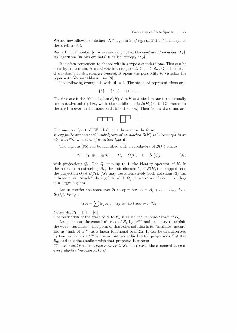
The following example is with |d| = 3. The standard representations are

3, 2, 1, 1, 1, 1 .

The first one is the “full” algebra B(H), dimH = 3, the last one is a maximallycommutative subalgebra, while the middle one is B(H2) ⊕ C. (C stands forthe algebra over an 1-dimensional Hilbert space.) Their Young diagrams are

One may put (part of) Wedderburn’s theorem in the form:Every finite dimensional ∗-subalgebra of an algebra B(H) is ∗-isomorph to analgebra (85), i. e. it is of a certain type d.

The algebra (85) can be identified with a subalgebra of B(H) where

H = H1 ⊕ . . .⊕Hm, Hj = QjH, 1 =∑

Qj , (87)

with projections Qj . The Qj sum up to 1, the identity operator of H. Inthe course of constructing Bd, the unit element 1j ∈ B(Hj) is mapped ontothe projection Qj ∈ B(H). (We may use alternatively both notations. 1j canindicate a use “inside” the algebra, while Qj indicates a definite embeddingin a larger algebra.)

Let us restrict the trace over H to operators A = A1 + . . . + Am, Aj ∈B(Hj). We get

trA =∑

trj Aj , trj is the trace over Hj .

Notice dimH = tr1 = |d|.The restriction of the trace of H to Bd is called the canonical trace of Bd.

Let us denote the canonical trace of Bd by trcan and let us try to explainthe word “canonical”. The point of this extra notation is its “intrinsic” nature:Let us think of trcan as a linear functional over Bd. It can be characterizedby two properties: trcan is positive integer valued at the projections P 6= 0 ofBd, and it is the smallest with that property. It means:The canonical trace is a type invariant. We can recover the canonical trace inevery algebra ∗-isomorph to Bd.


There is yet another aspect to consider. The Luders-von Neumann, orprojective measurements, [14], [50], [5], are in one-to-one correspondence withthe partition of the identity (87) of H. We can associate

d = d1, . . . , dm, dj = rank(Qj) (88)

with the measurement. The average measurement result is given by a tracepreserving and unital completely positive map13,

A → Φ(A) :=∑

QjAQj , A ∈ B(H) . (89)

In the direct sum (85), the term B(Hj) can be identified with QjB(H)Qj , thealgebra of all operators which can be written QjAQj . Hence,

Bd1,...,dm:=

⊕QjB(H)Qj , dj = rank(Qj) . (90)

→ Φ maps B(H) onto Bd .

Remark: Φ is a completely positive unital map which maps the algebra ontoa subalgebra, though it does not preserve multiplication: Generally QABQis not equal to QAQBQ with a projection Q. Several interesting questionsappear. For instance, which channels result after several applications of pro-jective ones? The problem belongs to the theory of conditional expectations.

The state space of Bd

To shorten notation we shall write Ω(H) instead of Ω(B(H)).Let us now examine the state space Ω(Bd) which is a subset of Ω(H). Indeed,a state ω of Bd can be written ω(A) = tr ωA and we conclude

tr ωA = tr ω∑

QjAQj = tr (∑

QjωQj)A

by (87). Hence we can choose ω ∈ Bd and, after doing so, ω becomes unique.In conclusion, Ω(Bd) ⊂ Ω(H) and

ω ∈ Ω(Bd) ⇔∑

QjωQj = ω (91)

for density operators ω ∈ Ω(H).A density operators ωj of B(Hj) can be identified with a density operators

on H supported by Hj = QjH. Equivalently we have ωj(Qj) = 1 for thecorresponding states. These states form a face of Ω(H), and these faces areorthogonal one to another. We get the convex combination

ω ∈ Ω(Bd) ⇔ ω =m∑

j=1

pjωj , tr Qjωj = ωj(Qj) = 1 . (92)

13 Complete positive maps respect the superposition principle in tensor products,[15], [5].


The convex combination (92) is uniquely determined by ω, a consequence ofthe orthogonality ωjωk = 0 if j 6= k.→ The state space of Bd, embedded in Ω(H), dimH = |d|, is the direct convexsum of the state spaces Ω(Hj) with dimHj = dj and dj ∈ d.We see further: Φ defined in (89) maps Ω(H) onto Ω(Bd).

A picturesque description is in saying we have a simplex with m cornersand we “blow up”, for all j, the j-th corner to the convex set Ω(Hj). Thenwe perform the convex hull.

From (87), (92), and the structure of Bd we find the pure (i. e. extremal)density operators by selecting j and a unit vector |ψ〉 ∈ Hj to be P = |ψ〉〈ψ|.(We may also write π = P , but presently we like to see the density operatorof a pure state as a member of the projections. This double role of rank oneprojectors is a feature of discrete type I von Neumann algebras.) Let π be thestate of Bd with density operator P . Just by insertion we see

PAP = π(A)P for all A ∈ Bd . (93)

On the other hand, if for any projector P there is a linear form π such that(93) is valid, π must be a state and P its density operator. (Inserting A = Pwe find π(P ) = 1. Because PA†AP is positive, π(A†A) must be positive.Hence it follows from (93), if P is a projection P , π is a state.) It is also notdifficult to see that (93) requires P to be of rank one and π is pure. We nowhave another criterium for pure states which refers to the algebra only.

Let A be ∗-isomorph to an algebra Bd. A state π of A is pure if and onlyif there is a projection P such that (93) is valid for all A ∈ A. Then P is thedensity operator of the pure state, or, in other terms, π = P .

The projections, which are density operators of pure states, enjoy a specialproperty, they are minimal. A projection P is minimal in an algebra, if fromP = P1 + P2 with Pj projections, it follows either P1 = P or P1 = 0.

It is quite simple to see P = |ψ〉〈ψ| for a minimal projection operator ofBd and, hence, it is a density operator of a pure state. Therefore in algebras∗-isomorph to an algebra Bd we can assert:A projection P of A is minimal if and only if it is the density operator of apure state of A.

A further observation: Let A be of type d. There is a linear functional overA which attains the value 1 for all minimal projections. This linear form isthe canonical trace of A.

By slightly reformulating some concepts from Hilbert space we have ob-tained purely algebraic ones. This way of thinking will also dominate our nextissue.


Transition probabilities for pure states

We start again with Bd as a subalgebra of B(H) with dimH = |d|. Let usconsider some pure states πj of Bd. They can be represented by unit vectors,

πj(A) = 〈ψj , Aψj〉, πj ≡ Pj = |ψj〉〈ψj | . (94)

Let us agree “as usual” that

Pr(π1, π2) = Pr(π1, π2) = |〈ψ1, ψ2〉|2 (95)

is the transition probability. To obtain the same value for two pure statesof an algebra A ∗-isomorph to Bd, we reformulate (95) in an invariant way:The right-hand side of (95) is the trace of π1π2. In Bd the canonical tracecoincides with the trace over H. Hence, for a general algebra A, we have touse the canonical trace. We get

Pr(π1, π2) = Pr(π1, π2) = trcanπ1π2 . (96)

Switching, for convenience, to the notation Pj = πj , we get P1P2P1 =π1(P2)P1 by inserting A = P2 in the appropriate equation (93) for π1. Bytaking the trace we get the expression (96) for the transition probability. In-terchanging the indices we finally get

Pr(π1, π2) = Pr(π1, π2) = π1(P2) = π2(P1) . (97)

This and (96) express the transition probability for any two pure states of analgebra A, ∗-isomorph to a finite dimensional von Neumann algebra.

Our next aim is to prove

Pr(π1, π2) = infA>0

π1(A)π2(A−1) , (98)

A is running through all invertible positive elements of A.It suffices to prove the assertion for Bd. Relying on (94) we observe

|〈ψ1, ψ2〉|2 ≤ 〈A1/2ψ1, A1/2ψ1〉〈A−1/2ψ2, A

−1/2ψ2〉 .

Therefore, the left-hand side of (98) cannot be larger than the right one. Itremains to ask, whether the asserted infimum can be reached. For this purposewe set

As = s1 + P2, A−1s =

1s1− 1

s(1 + s)P2 .

As is positive for s > 0. We find

π1(As) = s + Pr(π1, π2), π2(A−1s ) =

1s− 1

s(1 + s)= (1 + s)−1

and it follows


lims→+0

π1(As)π2(A−1s ) = Pr(π1, π2)

and (98) has been proven.In [1] a similar inequality is reported:

2|〈ψ1, ψ2〉| = infA>0

〈ψ1, Aψ1〉+ 〈ψ2, A−1ψ2〉

with A varying over all invertible positive operators on a Hilbert space. Theequation remains valid for pairs of pure states in a finite ∗-subalgebra A ofB(H). The slight extensions of the inequality reads

2√

Pr(π1, π2) = inf0<A∈A

π1(A) + π2(A−1) . (99)

To prove it we write out the inequality

0 ≤ (t√

π1(A)− t−1√

π2(A−1))2 ,

t a positive number. We get

2√

π1(A)π2(A−1) ≤ t2π1(A) + t−2π2(A−1)

and, by (98), the right-hand side of (99) is not less than the left one. Adjustingthe operators As above to Bs = t2sAs in such a way that π1(Bs) = π2(A

−1),then

2√

π1(Bs)π2(B−1s ) = π1(Bs) + π2(B

−1s ) .

Performing the limes s → 0 as in the proof of (98) shows that the assertedinfimum can be approached arbitrarily well.

Last not least we convince ourselves that the transition probability be-tween pure states is already fixed by the convex structure of Ω(A) respectivelyof Ω(A).

We prove it for Ω(A). Let l be a real linear form over the Hermitianoperators of A such that for all density operators ω one has 0 ≤ l(ω) ≤ 1.Then l(A) ≥ 0 for all positive operators A. Now assume l(P ) = 1 for a minimalprojection. Combining both assumptions we find l(1A) = 1. Hence l is a purestate π of A. If P ′ is another minimal projection, i. e. an extremal element ofΩ(A), we can calculate the transition probability l(P ′) = π(P ′).

The result implies: Our state spaces are rigid: If a linear map Φ,

Φ : A 7→ A ,

maps Ω(A) one–to–one onto itself, it must preserve the transition probabilitiesbetween pure density operators.

In the particular case A = B(H) the map Φ must be a Wigner symmetry.A useful reformulation of this statement reads:Let Φ1, Φ2 denote invertible linear maps from B(H) onto B(H). Assume Ω(H)


is mapped by both maps onto the same set of operators. Then there is a unitaryor an anti-unitary V such that

Φ2(X) = Φ1(V XV ∗) for all X ∈ B(H) .

Indeed, Φ−11 Φ2 must be a Wigner symmetry.

Remark: Mielnik has defined a “transition probability” between extremalstates of a compact convex set K in this way. Let P and P ′ be two extremalpoints of K. The “probability” of the transition P → P ′ is defined to beinf l(P ′) where l runs through all real affine functionals on K with valuesbetween 0 and 1 and with l(P ) = 1. Indeed, for Ω(A) the procedure gives thecorrect transition probability as shown above.

2.4 All subsystems for dim H < ∞

Here we are interested in Wedderburn’s description, of the ∗-subalgebras ofB(H), dimH < ∞, [21, 37]. In short, such a subalgebra is ∗-isomorph to acertain algebra Bd.

We change our notations towards its use in quantum information. We thinkof a quantum system with algebra BA, owned by some person, say Alice. Wemay assume the algebra BA to be a unital ∗-subalgebra of a larger algebraB(HAB). The type of BA is the not ordered list dA = dA

1 , . . . , dAm. Alice

is allowed to operate freely within her subsystem, which is also called “theA-system”.Theorem: Let BA be a unital ∗-subalgebra of B(HAB) of type dA. ThenThere is a decomposition

HAB = H1 ⊕ . . .⊕Hm, Hj = HAj ⊗HB

j , (100)

dAj = dimHA

j , dBj := dimHB

j ,

such thatBA = (B(HA

1 )⊗ 1B1 )⊕ . . .⊕ (B(HA

m)⊗ 1Bm) . (101)

Equally well we may represent BA as a diagonal block matrix with diagonalblocks B(HA

j )⊗ 1Bj .

In the theorem we denote by 1Aj the identity operator of HA

j and by 1Bj

the one of HBj . Therefore, 1A

j ⊗ 1Bj is equal to 1j , the identity operator of

Hj . The latter can be identified with the projection Qj projecting H onto Hj ,i. e. 1j = Qj . (100) and (101) describe how BdA is embedded into B(HAB) tobecome BA by the embedding ∗-isomorphism

A1 + . . . + Am ↔ A1 ⊗ 11 + . . . + Am ⊗ 1m, Aj ∈ B(HAj ) . (102)

Now we can see, why, by identifying BA as a subsystem of B(HAB), asecond subsystem, called “Bob’s system”, appears quite naturally. It consists


of those operators of B(HAB) which can be executed independently of Alice’sactions. These operators must commute with those of the A-system. Hence,all of them14 constitute Bob’s algebra, BB. Therefore, Bob’s algebra is thecommutant of BA in B(HAB). By (101) we see

BB := (BA)′ = (1A1 ⊗ B(HB

1 ))⊕ . . .⊕ (1Am ⊗ B(HB

m)) . (103)

We further can find the center of BA, respectively of BB. The center describesthe actions which are allowed to both, Alice and Bob. These operators behave“classical” for them. We get

BA ∩ BB = CQ1 + . . . + CQm, Qj = 1Aj ⊗ 1B

j = 1j . (104)

The type of the commutant consists of m-times the number one.The types of BA and of BB are dA = dA

1 , . . . , dAm and dB = dB

1 , . . . , dBm

respectively. In general, neither one can be assumed decreasingly ordered.Notice

dimHAB =∑

dAj dB

j .

Let us denote by BAB the subalgebra generated by BA and BB. Equiva-lently, BAB is the smallest subalgebra of B(H) containing BA and BB,

BAB = B(H1)⊕ . . .⊕ B(Hm) = Q1B(H)Q1 + . . . + QmB(H)Qm . (105)

The fact that BAB is generated in a larger algebra by the algebras BA and BB

can be expressed also by BAB = BA ∨ BB. The type of BAB is

dAB := dA1 dB

1 , . . . dAmdB

m .

As long as BAB is not considered itself as a subsysstem of a larger one, andwe are allowed to write BAB = BdAB .

Embedding and partial trace

Let us stick to the just introduced subalgebras of B(HAB), namely BA, BB,BAB, and C = BA ∩ BB.

If ωAB is a state of BAB, its restriction to BA is a state ωA of BA. Therestriction map lets fall down any functional of BAB to BA. After its appli-cation, we have obtained ωA from ωAB and all what has changed is: Onlyarguments from BA will be allowed for ωA.

The partial trace15, ωAB → ωA , concerns the involved density operators.It is a map from BAB to BA. For its definition and for later use we needthe canonical traces of BA and BB which we now denote by trA and trB

respectively. It is

14 We ignore that there may be further restrictions to Bob.15 The partial trace is a particular “conditional expectation”.


trAωAX = ωAB(X) ≡ tr ωABX, X ∈ BA . (106)

Remark: The algebra BAB is of the form (90), (85). Therefore, its canonicaltrace, trAB is the canonical trace over B(H), i. e. it is just the trace over H.

We read (106) as follows: The right-hand side becomes a linear form overBA. Every linear functional over BA can be uniquely written by the help ofthe canonical trace as done at the left-hand side. This defines the partial trace

ωAB → ωA := trBωAB (107)

from BAB to BA. The partial trace is “dual” to the restriction map.

The algebra BAB consists of all operators

Z =m∑

j=1

XjYj =m∑

j=1

(Aj ⊗ 1Bj ) (1A

j ⊗Bj) (108)

withAj ∈ B(HA

j ), Bj ∈ B(HBj ) .

This follows from (100) and (101). Now

trYj = tr (1Aj ⊗Bj) = dA

j trBj = dAj trBYj . (109)

The dimensional factors point to the main difference between the canonicaltrace of BA and of the induced trace, which is the trace of H applied to theoperators of the subalgebra BA. All together we get the partial trace of theoperator (108),

trB Z =∑

(dAj )−1(trYj)Xj =

∑Xj trBYj . (110)

An important conclusion is

trB XZ = XtrBZ, trB ZX = (trBZ)X, X ∈ BA. (111)

Similar to trB one treats the partial trace trA. One can check

trB trA = trA trB = trAB . (112)

Because trAB projects an operator of BAB into both, BA and BB, it projectsonto the center, C = BA ∩ BB, of BAB. By inspection we identify (112) withthe partial trace of BAB onto its center.

The ansatz (106) applies also to the partial trace from B(HAB) to BAB.Because the latter is the commutant of the center C = BA ∩ BB, we have

trA∩B(Z) =∑

QjZQj , BA ∩ BB =∑

QjC , (113)

see (87) and (89), where the map has been called Φ because at this occasionthe partial trace was not yet defined.


3 Transition probability, fidelity, and Bures distance

The aim is to define transition probabilities, [59], [46], between two states ofa quantum system, say A, by operating in larger quantum systems. We callit Pr(ρ, ω) or, with density operators, Pr(ρ, ω).

The notation for the fidelity, F(ρ, ω), used here is that of Nielsen andChuang16, [15], i. e. it is the square root of the transition probability,

F(ρ, ω) :=√

Pr(ρ, ω) . (114)

This quantity is also denoted by “square root fidelity” or by “overlap”. Ananalogous quantity between two probability measures is known as “Kaku-tani mean”, [47], and, for probability vectors, as “Bhattacharyya coefficient”.Occasionally the latter name is also used in the quantum case.

There is a related extension of the Study-Fubini distance to the Bures one,[34]. The Bures distance, distB(ρ, ω), is an inner distance in the set of positivelinear functionals, or, in finite dimensions equivalently, in the set of positiveoperators. The Bures distance is a quantum version of the Fisher distance,[40].

There is a Riemannian metric, the Bures metric, belonging to the Buresdistance, [61]. It extends the Fubini-Study metric to general (i.e. mixed) states.It also extends the Fisher metric, originally defined for spaces of probabilitymeasures, to quantum theory. (However, there is a large class of reasonablequantum versions of the Fisher metric, discovered by Petz, [53].)

Below we shall define transition probability and related quantities “oper-ationally”. Later we shall discuss several possibilities to get them “intrinsi-cally”, without leaving a given quantum system, [59], [46].

From the mathematical point of view, there are some quite useful tricksin handling two positive operators in general position.

3.1 Purification

Purification is a tool to extend properties of pure states to general ones. Itlives from the fact that, given a state, say ωA, of a quantum system A, thereare pure states in sufficiently larger systems the restriction of which to the A-system coincides with ωA. The same terminology is used for the correspondingdensity operators. Of special interest is the case of a larger system whichpurifies all states of the A-system.

We can lift any state of a quantum system to every larger system. We canrequire that a pure state is lifted to a pure state:Let A1 ⊂ A2 ⊂ B(H) and π1 a pure state of A1 with density operator P1.Being a minimal projection in A1, P1 may be not minimal in A2. But thenwe can write P1 as a sum of minimal projections of A2. If P2 is one of themand π2 the corresponding pure state of A2, then π2 is a pure lift of π1.16 There are also quite different expressions called “fidelity”.


As a matter of fact, every state ω2 satisfying ω2(P1) = 1 is a lift of π1 toA2. These states exhausts all lifts of π1 to A2. They constitute a face of thestate space of A2.Assume the state ω1 of A1 is written as a convex combination of pure states.After lifting them to pure states of A2 we get a convex combination whichextends ω1 to A2.Generally, there is a great freedom in extending states of a quantum systemto a larger quantum system.

The most important case is the purification of the states of B(H) or, equiv-alently, of Ω(H), well described in [9], [15], [4], [19], and in other text books onquantum information theory. It works by embedding B(H) as the subalgebraB(H)⊗ 1′ into a bipartite system B(H⊗H′), provided d = dimH ≤ dimH′.Given ω ∈ Ω(H), a unit vector ψ ∈ H ⊗H′ is purifying ω, and π = |ψ〉〈ψ| isa purification of ω, if

〈ψ, (X ⊗ 1′)ψ〉 = tr Xω for all X ∈ B(H) (115)

or, equivalently,ω(X) = π(X ⊗ 1′) ≡ trπ(X ⊗ 1′) . (116)

To get a suitable ψ, one chooses d ortho-normal vectors |j〉′ in H′ and a basis|j〉 of eigenvectors of ω. Now

|ψ〉 =∑

λ1/2|j〉 ⊗ |j〉′ with ω|j〉 = λj |j〉 (117)

purifies ω. Indeed,

〈ψ, (X ⊗ 1′)ψ〉 =∑

λj〈j|X|j〉 = tr Xω .

Now let A be a unital ∗-subalgebra of B(H) and ωA one of its states. Wehave already seen that we can lift ωA to a state ω of B(H). With the densityoperator ω of ω we now proceed as above.

3.2 Transition probability, fidelity, ...

Let A be a unital ∗-subalgebra of an algebra B(H) with finite dimensionalHilbert space H. Denote by ωA

1 and ωA2 two states of A and by ωA

1 and ωA2

their density operators.The task is, to prepare ω2 if the state of our system is ω1.

To do so one thinks of purifications πj of our ωAj in a larger quantum system

in which A is embedded.One then tests, in the larger system, whether π2 is true. If the answer of thetest is “yes”, then π2 and, hence, ωA

2 is prepared.The probability of success is Pr(π1, π2) as defined in (95), (96), and (97).


One now asks for optimality of the described procedure, i.e. one looks fora projective measurement in a larger system which prepares a purification ofωA

2 with maximal probability.This maximal possible probability for preparing ωA

2 with given ωA1 is called

the transition probability from ωA1 to ωA

2 or, as this quantity is symmetric in itsentries, the transition probability of the pair ωA

1 , ωA2 . The definition applies

to any unital C∗-algebra and, formally, to any unital ∗-algebra, [59, 27].The definition can be rephrased

Pr(ωA1 , ωA

2 ) := sup Pr(π1, π2) , (118)

where π1, π2 is running through all simultaneous purifications of ωA1 , ωA

2 . Wealso use the density operator notation

Pr(ωA1 , ωA

2 ) ≡ Pr(ωA1 , ωA

2 ) .

In almost the same way we define the fidelity by

F(ω1, ω2) = sup |〈ψ1, ψ2〉| (119)

where ψ1, ψ2 run through all simultaneous purifications of ω1, ω2 in someB(H). Though, we do not include all possible purifications, (by using only“full” algebras,) the relation (114) remains valid.Remark: Let ω1, ω2 two states of a unital C∗-algebra A and ν one of its alinear functionals. If and only if

|ν(A†B)|2 ≤ ω1(A†A) ω2(B

†B) (120)

for all A, B ∈ A there is an embedding Ψ in an algebra B(H) such that thereare purifying vectors ψ1, ψ2 satisfying

ν(A) = 〈ψ1, Ψ(A)ψ2〉, A ∈ A . (121)

This relation implies|ν(1)|2 ≤ Pr(ω1, ω2) . (122)

Now the definition above can be rephrased: The transition probability is thesup of |ν(1)|2 with ν running through all linear forms satisfying (121). Thereexist linear functionals ν satisfying (120) with equality in (122). Their struc-ture and eventual uniqueness has been investigated by Alberti, [26].

The Bures distance

For the next term, the Bures distance, [34], it is necessary, not to insist innormalization of the vectors and not to require the trace one condition for thedensity operators in (119).Remembering (28) and (29), one defines the Bures distance by


distB(ω1, ω2) = sup distFS(π1, π2) = sup ‖ ψ2 − ψ1 ‖ (123)

where the sup is running through all simultaneous purifications of ω1 and ω2.Because of (119) this comes down to

distB(ω1, ω2) =√

trω1 + tr ω2 − 2F(ω1, ω2) . (124)

Rewritten for two density operators it becomes


2− 2√

Pr(ω1, ω2), trωj = 1 .

If only curves entirely within the density operators are allowed in opti-mizing for the shortest path, we get a further variant of the Bures distance,namely

DistB(ω1, ω2) = arccos√

Pr(ω1, ω2) (125)

in complete analogy to the discussion of the Study-Fubini case.

What remains is to express of (118) or (119) in a more explicit way. Thedangerous thing in these definitions is the word “all”. How to control allpossible purifications of every embedding in suitable larger quantum systems?The answer is in a “saturation” property: One cannot do better in (118) thanby the squared algebraic dimension of A for the purifying system.

3.3 Optimization

Let A = Bd with d = |d| as in (85) and (87). Hence, up to a slight change innotation we have

A = B(HA1 )⊕ B(HA

2 )⊕ . . .⊕ B(HAm) , (126)

HA = HA1 ⊕ . . .⊕HA

m .

A ⊂ B(HA) is an embedding with the least possible Hilbert space dimension.(In contrast to (101), the general case.) Our working space will be

HAB = HA ⊗HB, dimHB = dimHA = d . (127)

The production of purifying vectors is simplified by first selecting a maximallyentangled vector

|ϕ〉 =d∑

j=1

|jj〉 ≡∑

|j〉A ⊗ |j〉B (128)

of length d. |j〉A and |j〉B are bases of HA and of HA respectively. Forany X ∈ B(HA) we get

(X ⊗ 1A)|ϕ〉 =∑

X|j〉A ⊗ |j〉B .


Bases are linearly independent. Hence if the right-hand side is zero, thenX = 0. Because the dimension of B(Ha) as a linear space is equal to thedimension of the Hilbert space (127), every vector ψ in HAB has a uniquerepresentation (X ⊗ 1)|ϕ〉.One computes for X1, X2 ∈ B(HA) the partial trace

ψi = (Xi ⊗ 1)|ϕ〉 ⇒ trB|ψ1〉〈ψ2| = X1X†2 , (129)

because we have to trace out the B-system in∑

X1(|j〉A〈k|)X†2 ⊗ (|j〉B〈k|) .

Our choice of A implies Ω(A) ⊂ Ω(HA), see (91) and (92). Therefore, wecan apply (129) above to the density operators of the A-system. Now let ωA

be a density or just a positive operator from A. It is convenient to call anoperator W ∈ A an amplitude of ωA if ωA = WW ∗. (W ⊗1)|ϕ〉 is a purifyingvector for ωA if W is an amplitude of ωA and vice versa.

There are many amplitudes of ωA and the change from one to another onecan be described17 by gauge transformations W → W ′ = WU with unitaryU ∈ A. The gauge transformations respect ωA as a gauge invariant.

Let us return to our problem with two density operators, ωA1 and ωA

2 , andtwo purifying vectors, ψ1 and ψ2. There are two operators W1, W2 in our Asatisfying

ψj = (Wj ⊗ 1)ϕ, ωAj = WjW

†j . (130)

With these amplitudes we have

〈ψ1, ψ2〉 = 〈(W1 ⊗ 1)ϕ, (W2 ⊗ 1)ϕ〉 = tr W †1 W2 . (131)

Gauging ψ2 → ψ′2 by W2 → W ′2 = W2U , we see

〈ψ1, ψ′2〉 = tr W †

1 W2U .

Let us stress that we fix W1 and vary only W2 in this relation. Hence

F (ωA1 , ωA

2 ) = supψ′|〈ψ1, ψ

′2〉| = sup

U∈A|trW †

1 W2U | ,

provided one cannot get better results in higher dimensional purifications. Butthis is not the case, as one can prove. (Essentially, this is because the largestdimension of a cyclic representation of B(HA) is of dimension d2.)

It is |tr BU | ≤ tr B in case B ≥ 0 and U is unitary. Hence we are done ifW †

1 W2 ≥ 0 can be reached. This is possible because the polar decomposition

17 due to our finiteness assumptions


theorem is valid in A (and, indeed, in every von Neumann algebra). In otherwords, we can choose a pair of amplitudes such that

F (ωA1 , ωB

2 ) = tr W †1 W2, W †

1 W2 ≥ 0 . (132)

Let us restate (132) to respect ∗-isomorphisms. If A is any (finite dimensional)∗-subalgebra of any B(H), we have to understand the trace in (132) as thecanonical trace. (Remember: Only for the algebras Bd with dimH = d thecanonical trace coincides with the trace of H.)Whenever for two density operators of A

ωA1 = W1W

†1 , ωA

2 = W2W†2 , W †

1 W2 ≥ 0 ,

we call the pair of amplitudes W1, W2 parallel. Parallelity implies

F(ωA1 , ωA

2 ) = trcan W †1 W2, Pr(ωA

1 , ωA2 ) = (trcan W †

1 W2)2 . (133)

3.4 Why the Bures distance is a distance

Before proceeding along the main line the triangle inequality should be proved.Inserting (132) into (124) yields:

distB(ωA1 , ωA

2 ) =√

trW1W†1 + trW2W

†2 − 2trW †

1 W2

Now observe that the traces of WW † and W †W are equal. Further remindthat W †

1 W2 is assumed to be positive and, therefore, hermitian:

W †1 W2 = W †

2 W1 . (134)

Altogether we proved: If W1, W2 are parallel amplitudes then

distB(ωA1 , ωA

2 ) =√

trcan (W1 −W2)†(W1 −W2) , (135)

and for two arbitrary amplitudes the left-hand side cannot be larger than theright one. The latter can also be rewritten ‖ W2 −W1 ‖2.

Consider now three positive operators, ωA1 , ωA

2 , and ωA3 . Starting with W2

we can choose W1 and W3 such that the pairs W2,W1 and W2, W3 are parallelamplitudes. This allows to convert the triangle inequality

‖ W1 −W2 ‖2 + ‖ W2 −W3 ‖2≥‖ W1 −W3 ‖2into

distB(ωA1 , ωA

2 ) + distB(ωA2 , ωA

3 ) ≥‖ W1 −W3 ‖2and the last term cannot be smaller than the Bures distance. Hence

distB(ωA1 , ωA

2 ) + distB(ωA2 , ωA

3 ) ≥ distB(ωA1 , ωA

3 ) . (136)


It is instructive to rewrite our finding with purifying vectors. We extendour notation and call a pair of purifying vectors parallel if the amplitudes in(130), that is in ψj = (Wj ⊗ 1)ϕ, are parallel ones. We can express (135) by

distB(ωA1 , ωA

2 ) ≤‖ ψ2 − ψ1 ‖ (137)

for all pairs of purifying vectors of ωA1 , ωA

2 . Equality holds for pairs of parallelpurifying vectors.

Some geometric properties of the Bures distance

The Bures distance is an inner one: There are short geodesic arcs with lengthequal to the Bures distance of their end points. Given ωA

0 , ωA1 we choose par-

allel amplitudes W0,W1. Then any pair of amplitudes belonging to the arc

t 7→ Wt = (1− t)W0 + tW1, 0 ≤ t ≤ 1, (138)

is a parallel pair. Exactly as in (10) we get

distB(ωAs , ωA

t ) =‖ Wt −Ws ‖2, ωAs = WsW

†s . (139)

Bures did not ask wether his distance is based on a Riemannian metric. Hewas interested in cases with infinite tensor products of von Neumann algebrasand the theory of infinite dimensional manifolds had not been developed. Butfor finite dimension it is tempting to ask for.

There is, indeed, a Riemannian metric reproducing the Bures distance. Itsline element is given by

(dsB

dt

)2 = trcan G2ωA =12trcan ωAG , (140)

whenever there is a solution of

ωA = ωAG + GωA, G = G† . (141)

For invertible positive operators ωA there is a unique solution of (141). Atthe boundary, where the rank is smaller than the Hilbert space dimension,the existence of G depends on the direction of the tangent ωA. For dimH ≥ 3there are directions for which the metric becomes singular [36].

However, for invertible ωA the metric behaves regularly. Let

t → ωAt = WtW

†t , |ψt〉 = (Wt ⊗ 1B)|ϕ〉, (142)

be an arc of invertible density operators. The the curve t → Wt of the ampli-tudes are called parallel, if

W †t Wt = W †

t Wt . (143)


By straightforward computation one proves the equivalence of (141) with thecondition

Wt = GtWt, G†t = Gt . (144)

Now one easily gets

t → Wt parallel, ⇒ (dsB

dt

)2 = trcan WW † . (145)

It is an easy nice exercise to compute the Bures distance (139) by (145) toestablish that the Bures distance can be gained from the metric (140).

After switching to the purifying arc |ψt〉 = (Wt ⊗ 1B)|ϕ another form ofthe results above appears: The Hilbert space length of a purifying lift t → |ψt〉of t → ωA

t is never less than its Bures length. Equality is reached exactly withparallel amplitudes (143) in (142).

The extended Mandelstam-Tamm inequality

An application is the extended Mandelstam-Tamm inequality . Let be

t → ωt, 0 ≤ t ≤ 1 (146)

a solution of time dependent von Neumann - Schrodinger equation

ihω = [H, ω], H = Ht . (147)

Then one can prove∫ 1

0

dt√

tr(ωH2)− (tr ωH)2 ≥ h arccos F(ω1, ω0) , (148)

see [60]. (One has to look for a lift t → Wt satisfying the differential parallelcondition W †W = W †W and a Schrodinger equation with an HamiltonianW → HW + WH, where t → Ht has to be chosen suitably.)

Using this one can get a differential form of (148) :

tr(ωH2)− (tr ωH)2 ≥ h

2trGω . (149)

One may compare this inequality with the “quantum Rao-Cramers in-equality”, which, however, plays its role in a quite different context (hypothe-sis testing and other questions of mathematical statistics). A recent overview,discussing these relationships, is in I. Bengtsson’s paper [32]. Another questionhas been discussed by A. Ericsson, [39].


3.5 Expressions for fidelity and transition probability

Now we return to (132) and (133) to benefit from the positivity of W †1 W2 for

parallel amplitudes. It holds

(W †1 W2)2 = W †

1 W2W†2 W1 = W †

1 ωA2 W1 .

There is a polar decomposition

W1W†1 = ωA

1 , W1 = (ωA1 )1/2U1

with a unitary U1. Putting things together yields

(W †1 W2)2 = U−1

1 (ωA1 )1/2ωA

2 (ωA1 )1/2U1 (150)

we can take the positive root and obtain

W †1 W2 = U−1

1

√(ωA

1 )1/2ωA2 (ωA

1 )1/2 U1 (151)

The canonical trace of (151) yields the fidelity,

F(ωA1 , ωA

2 ) = trcan√

(ωA1 )1/2ωA

2 (ωA1 )1/2 , (152)

its square is the transition probability.

As an application we consider direct products. With two pairs, ω1, ω2 andρ1, ρ2 of density operators in two different Hilbert spaces, one can performtheir direct products ωj ⊗ ρj . The structure of the expression (152) allows toconclude

Pr(ω1 ⊗ ρ1, ω2 ⊗ ρ2) = Pr(ω1, ω2) Pr(ρ1, ρ2) . (153)

In what follows we assume invertible positive operators though the resultsdo not depend on that assumption. As above W1,W2 are parallel amplitudesof ωA

1 , ωA2 . We define a positive gauge invariant, K,

W †1 W2 > 0 ⇔ W2 = KW1, K > 0 . (154)

Indeed, W †1 W2 = W †

1 KW1 proves K > 0 equivalent to parallelity. Now

K = W2W−11 > 0, K−1 = W1W

−12 > 0, (155)

and we conclude the existence of K ∈ A such that

trcanωA1 K = trcanW †

1 W2 = trcanωA2 K−1 . (156)

But trcanW †1 W2 is the fidelity and with our K we have


F(ωA1 , ωA

2 ) = trcanωA1 K = trcanωA

2 K−1 (157)

For a pair ψ1, ψ2 of parallel purifications and for every positive C ∈ B(HA ⊗HB) we know from (99)

F(ωA1 , ωA

2 ) = |〈ψ1, ψ2〉| ≤ (1/2)(〈ψ1, Cψ1〉+ 〈ψ2, C−1ψ2〉)

Inserting C = X⊗1B it becomes clear, that the right-hand side cannot becomesmaller than

12

infX>0

(tr ω1X + tr ω2X−1), X ∈ A .

The particular case X = K proves

F(ωA1 , ωA

2 ) =12

infX>0

(tr ωA1 X + trωA

2 X−1) . (158)

Let us reformulate (158) to change from density operators to states. Finallythere is no reference on any bipartite structure.Let A be a ∗-subalgebra of B(H) and ω and ρ two of its states or positivelinear forms. Then

F(ω, ρ) =12

inf0<X∈A

ω(X) + ρ(X−1) , (159)

Pr(ω, ρ) = inf0<X∈A

ω(X) ρ(X−1) . (160)

Thanks to the work of Araki and Raggio, [25], and Alberti, [24], the two lastassertions are known to be true for any pair of states of any unital C∗-algebra.

Super-additivity

For all decompositions

ω =∑

ωj , ρ =∑

ρj (161)

of positive operators the inequality

F(ω, ρ) ≥∑

j

F(ωj , ρj) (162)

is valid. The inequality expresses “super-additivity” of the fidelity.For simplicity we prove super-additivity assuming ω and ρ invertible and

choose K ∈ A satisfying

F(ω, ρ) = trcanωK = trcanρK−1

as in (156) and (157). We now have


2F(ω, ρ) =∑

trcanωjK +∑

trcanρjK−1 .

The proof terminates by estimating the right part by (158). This is the finitedimensional case. (For von Neumann and C∗-algebras one returns to positivelinear forms for which super-additivity of the fidelity can be proved equallywell.)

Let us mention how (161) implies joint concavity. Because of

F(aω, bρ) =√

ab F(ω, ρ), a, b ∈ IR+ (163)

it follows from (161) for convex sums of equal length

F(∑

j

pjωj ,∑

k

qkρk) ≥∑

j

√pjqj F(ωj , ρj) . (164)

From (152) one can conclude: Equality holds in (164) if for j 6= k it holdsωjρk = 0. Similar (indeed equivalent) statements are true for (159) and (160).

Monotonicity

Choi, [35], proved for positive unital maps

Ψ(A−1) ≥ Ψ(A)−1 if A ≥ 0 . (165)

In the case of a 2-positive and unital Ψ the conclusion(

A CC† B

)≥ 0 ⇒

(Ψ(A) Ψ(C)Ψ(C†) Ψ(B)

)≥ 0 (166)

comes simply from the very definition of 2-positivity. Then (165) follows withB = A−1, C = 1 and unitality, Ψ(1) = 1. However, according to Choi, inthe particular case C ≥ 0 just positivity and unitality are sufficient for thevalidity of (166). Therefore, (165) is valid for positive unital maps.

Let us apply (165) to the fidelity. To this end we denote by Φ the mapdual to Ψ ,

trXΨ(Y ) = tr Φ(X)Y . (167)

Ψ is positive if Φ is positive. Φ is trace preserving if Ψ is unital. Not everypositive operator might be of the form Ψ(X) with positive X. Therefore, by(158) or (159),

F(ω, ρ) ≤ 12

inf0<X∈A

trcanΨ(X)ω + trcanΨ(X)−1ρ .

We can replace Ψ(X)−1 by the smaller Ψ(X−1) in virtue of (165) to get aneven larger right hand side:


F(ω, ρ) ≤ 12

inf0<X∈A

trcanΨ(X)ω + trcanΨ(X−1)ρ .

Now we apply duality, (167), and obtain

F(ω, ρ) ≤ 12

inf0<X∈A

trcanXΦ(ω) + trcanX−1Φ(ρ) .

The right-hand side is an expression for the fidelity of the pair Φ(ω), Φ(ρ) andthe proof of the monotonicity property is done:Let Φ be positive and trace preserving. Then

F(ω1, ω2) ≤ F(Φ(ω1), Φ(ω2)) . (168)

As a consequence, trace preserving positive maps are “Bures-contracting”,

distB(ω1, ω2) ≥ distB(Φ(ω1), Φ(ω2)) . (169)

Density operators (and states) become closer one to another under the actionof these maps.

Remark: It is well known that there are many Riemannian metrics in astate space Ω(H) which are monotone decreasing with respect to channels,i. e. with respect to completely positive and trace preserving maps18. Thanksto the work of Petz, [53], they can be constructed by the help of certainoperator means. Kubo and Ando,[49], could enumerate all operator means byoperator monotone functions. Another, but much related story is the questionfor functions Pr ′(., .), depending on two states, which area) monotone increasing with respect to channels and whichb) coincide with the transition probability for pure states.Some of them are related to distances, i. e. inserting in distB the square rootof Pr ′ for F returns a distance. Most of them, however, are not related toany distance. But what our alternative choice may be, only the transitionprobability (118) is “operational” defined. Just by this very definition onefinds, for pairs of density operators,

Pr(ω, ρ) ≥ Pr ′(ω, ρ) (170)

for all Pr′ satisfying the two condition a) and b) above. A nice example is

Pr(ω, ρ) ≥ tr ω1−sρs, 0 < s < 1 . (171)

Indeed, the right hand side fulfills a) and b) above, see [30], where one canalso find a more “direct” proof of (171).

18 Though their geodesics and distances are mostly unknown.


3.6 Estimates and a “hidden symmetry”

I use the notation

char(A) = all roots of the characteristic equation of A . (172)

Clearly, this are the eigenvalues, counted with the appropriate multiplicity, ifA is diagonalisable. Because of

ω1/21 (ω1/2

1 ω2ω1/21 )ω−1/2

1 = ω1ω2

one concludeschar(ω1/2

1 ω2ω1/21 ) = char(ω1ω2) . (173)

An estimate

Denoting the characteristic values of (173) by λ1, λ2, . . ., we get

Pr(ω1, ω2) = (∑ √

λj)2 . (174)

The sum of the λj is the trace of ω1ω2. Hence

Pr(ω1, ω2) = tr ω1ω2 + 2∑

j<k

√λjλk .

We write 2r for the last term and use

√r2 =

√∑

j<k

λjλk + . . . .

The dots abbreviate some non-negative terms. The other term in the sum isthe second elementary symmetric function of the characteristic values λk ofω1ω2. Expressing the latter by traces yields

Pr(ω1, ω2) ≥ tr ω1ω2 +√

2√

(trω1ω2)2 − tr(ω1ω2)2 (175)

with equality for rank(ω1ω2) ≤ 2. For dimH = 3 closer inspection produces

Pr(ρ, ω) = tr ρω +√

2√

(tr ρω)2 − tr(ρωρω) + 4F (ρ, ω)√

det(ρω) .

One qubit, dim H = 2

In the one qubit case (175) becomes an equality. λ1λ2 is the determinant ofω1ω2. Thus

Pr(ω1, ω2) = trω1ω2 + 2√

detω1 detω2 . (176)

Let us represent our density matrices by


ω1 =12(1 +

∑xnσn), ω2 =

12(1 +

∑ynσn) (177)

and let us define a new coordinate by

x4 := 2√

detω1, y4 := 2√

det ω2 . (178)

We have now placed the density operators on the upper 3-hemisphere,

x21 + . . . + x2

4 = y21 + . . . + y2

4 = 1 (179)

with x4 ≥ 0, y4 ≥ 0 . The transition probability becomes

Pr(ω1, ω2) =12(1 +

4∑

j=1

xjyj) . (180)

A “hidden symmetry”

Remember first the equality (173) for the characteristic numbers. Let Z beinvertible and consider the change

ω′1 = Z−1ω1(Z−1)†, ω′2 = Z†ω2Z . (181)

One immediately seesω′1ω

′2 = Z−1(ω1ω2)Z (182)

andchar(ω′1ω

′2) = char(ω1ω2) . (183)

Now (173) implies:The eigenvalues of

√ω1ω2

√ω1 do not change if ω1, ω2 are transformed ac-

cording to (181). In particular

F (ω1, ω2) = F (Z−1ω1(Z−1)†, Z†ω2Z) . (184)

Indeed, the argument is valid for every symmetric function of the character-istic numbers in question. We can even refrain from the invertibility of Z by

substitutingω1 → Zω1Z

†

in (184):F (Zω1Z

†, ω2) = F (ω1, Z†ω2Z) . (185)

Relaying on continuity we can state (185) for all operators Z.


3.7 “Operational fidelity”

The question is, whether the fidelity concept can be extended to pairs ofquantum channels. It seems, the first relevant studies are done by Raginski,[55]. More recent developments can be seen from Belavkin et al., [31], andKretschmann et al., [48]. Essentially, our aim is to define what is called opera-tional fidelity and to arrive at it via the Bures distance. We restrict ourselvesto maps Φ from B(H) into itself, and we assume dimH = d finite.

We denote by I the identity map I(X) = X, X ∈ B(H). Later on we needthe identity maps Ik of auxiliary algebras B(Hk) with dimHk = k.

With two positive maps, Φ1 and Φ2, and a density operator ω ∈ Ω(H) weobserve that

Φ1, Φ2 → distB(Φ1(ω), Φ2(ω))

is symmetric in the maps and fulfils, for three positive maps, the triangleinequality. This is because the Bures distance does so. As Φ1(ω) = Φ2(ω)may happen, we do not necessarily get a metrical distance, but only a “semi-distance”. As one can check, the sup of arbitrary many semi-distances is againa semi-distance. Therefore,

dist1(Φ1, Φ2) := supω∈Ω

distB(Φ1(ω), Φ2(ω)) (186)

is a distance in the space of positive maps.Indeed, as said above, it is a semi-distance. But if two maps are not equalone to another, there must be a density operator at which they take differentvalues. The index “1” in (186) reflects our assumption that the maps are justpositive, i. e. 1-positive. Obviously, the distance dist1(Φ, I) estimates howstrongly Φ deviates from the identity map.

If a map Φ is k-positive, then the map Φ⊗ Ik is still positive. For pairs ofk-positive maps the expression

distk(Φ1, Φ2) := dist1(Φ1 ⊗ Ik, Φ2 ⊗ Ik) (187)

is well defined. More explicitly, (187) is a sup,

supρ

distB([Φ1 ⊗ Ik](ρ), [Φ2 ⊗ Ik](ρ)) , (188)

over all density operators ρ ∈ Ω(H⊗Hk).One can unitarily embed H ⊗ Hk into H ⊗ Hk+1. This implies that the

sup in (188) is running over less states as in the case distk+1, resulting in

distk(Φ1, Φ2) ≤ distk+1(Φ1, Φ2) . (189)

This enables the introduction of an operational Bures distance

dist∞(Φ1, Φ2) := limk→∞

distk(Φ1, Φ2) (190)


which takes into account possible entanglement in the input. Possible entan-glement based on H⊗Hk saturates with dimH = k,

dist∞(Φ1, Φ2) = distd(Φ1, Φ2), d = dimH . (191)

To obtain what has been called operational fidelity in the literature, we haveto go back to the relation (124)


trω1 + tr ω2 − 2F(ω1, ω2)

and try to replace accordingly states by maps. The task can be done quitenaturally for completely positive, trace preserving maps: For all these mapstrΦ(ω) = 1 for density operators. It suggests

dist∞(Φ1, Φ2) =√

2− 2F(∞)(Φ1, Φ2) . (192)

The quantity F(∞)(Φ1, Φ2) is called “operational fidelity”. The index (∞)is not standard and stands here only to respect the possibility of the sameprocedure with k-positive and trace preserving maps. For such maps one canconsider an “operational fidelity for k-positivity”, F(k), as well.

As a matter of fact, one can transmit several properties of the fidelity andthe Bures distance for states to completely or k-positive and trace preservingmaps. The joint concavity for instance allows to perform the sup in (186) orin (187) over pure states only.

4 Appendix: The geometrical mean

Let A, B, and C be positive operators in a finite dimensional Hilbert space. Aremarkable observation due to Pusz and Woronowicz, [54], can be rephrasedin the following form:

Given A ≥ 0 and B ≥ 0, there is a largest operator in the set of all Csatisfying (

A CC B

)≥ 0, C ≥ 0 . (193)

This unique element is called the geometrical mean of A and B and it will bedenoted, following Ando, by

A#B . (194)

In other words: (193) is valid if and only if

0 ≤ C ≤ A#B . (195)

From the definition we get the relation

A#B = B#A, A−1#B−1 = (A#B)−1 , (196)


the latter is true for invertible positive operators. If just A is invertible thenthe block matrix (193) is positive if and only if

B ≥ CA−1C (197)

and one concludes: A#B is the unique positive solution X of the equation

B = XA−1X, X ≥ 0 . (198)

The equation can be solved and one gets

A#B = A1/2(A−1/2BA−1/2)1/2A1/2 . (199)

To prove it, one rewrites (198) as

A−1/2BA−1/2 =(A−1/2XA−1/2

)2

and takes the root.In case B−1 exists too, we may rewrite (198) as

1 = B−1/2XA−1XB−1/2 = (B−1/2XA−1/2) (B−1/2XA−1/2)† .

Therefore, if A und B are strictly positive, the following three statements areequivalent: a) X = A#B, b) (B−1/2XA−1/2) is unitary, c) (A−1/2XB−1/2)is unitary.

In turn, as shown in [29], an operator X = (A1/2UB1/2) with unitary Uis positive exactly if X = A#B.

If A and B commute one can see from (193)

AB = BA ⇒ A#B = (AB)1/2 (200)

To get it one uses a common eigenbasis which reduces (193) to(

a cc b

)≥ 0 ⇔ ab ≥ c2

for three positive numbers a, b, and c.

4.1 Geometric mean and fidelity

Let us return to the operator K, defined in (154) by

W2 = KW1 if W †1 W2 > 0

for parallel and invertible amplitudes. One can calculate

K = ω−1/21 (ω1/2

1 ω2ω1/21 )1/2ω

−1/21 (201)


and conclude: At first we can rewrite (201)

K = ω2#ω−11 , (202)

and, secondly, the expression remains meaningful for not invertible ωj . In thissense we understand the right-hand side of (201) and (202) to be valid forall pairs of positive operators in our finite dimensional setting. One furtherconcludes that for general pairs of positive operators we have to substitute

K → ω2#ω−11 and K−1 → ω1#ω−1

2

in order that (156) and (157) can be applied to not necessarily invertiblepositive operators. With this convention one arrives at

Pr(ω1, ω2) = ω1(ω2#ω−11 ) = ω2(ω1#ω−1

2 )

For parallel purifications in HAB = HA ⊗ HA of states ωA1 and ωA

2 onemay ask, how these purifications appear in Bob’s system, i. e. after tracingout the A-system. To this end let us first review the general situation, notrequiring parallelity. We choose amplitudes, W1, W2, for ωA

1 and ωA2 , so that,

for m = 1, 2,

ωAj = WmW †

m = trB|ψm〉〈ψm|, |ψm〉 = (Wm ⊗ 1B)|ϕ〉 (203)

with |ϕ〉 chosen maximally entangled and with norm d = dimHA as in (128).For any Y ∈ B(HB) we get

tr (|ψn〉〈ψm|)BY = 〈ψm|(1A ⊗ Y )|ψn〉 = 〈ϕ|(W †mWn ⊗ Y )|ϕ〉 . (204)

The last expression is equal to∑

〈j|W †mWn|k〉〈j|Y |k〉 .

Let us define the transposition X → X> by

〈j|X>|k〉B = 〈k|X|j〉A . (205)

In this equation we used the two basis of the subsystems with which ϕ isrepresented in (128). It now follows

tr (|ψn〉〈ψm|)BY = tr (W †mWn)>Y

and, therefore,(|ψn〉〈ψm|)B = (W †

mWn)> . (206)

Next we conclude, for m = 1, 2,


ωBm := (|ψm〉〈ψm|)B = (W †

mWm)> . (207)

We are now prepared to use parallel amplitudes and proceed in showing

W †mWn ≥ 0 ⇒ W †

mWn = (W †mWm)#(W †

nWn) . (208)

At first we assume invertibility of Wm and use the identity

(W †nWn) = (W †

nWm)(W †mWm)−1(W †

mWn)

which is true for parallel amplitudes. According to (198) our assertion mustbe true. In the general case we mention that (193) forces the geometric meanA#B to give zero if applied to any null-vector of either A or B. Therefore,the support of A#B is the intersection of the supports of A and of B. ThusA and B become invertible if restricted onto the support of their geometricmean and the reasoning above applies.

We can now return to (208) and state:If Wm are parallel amplitudes for ωA

m then

W †1 W2 = (ωB

1 #ωB2 )> (209)

and, in particular,F (ωA

1 , ωA2 ) = tr (ωB

1 #ωB2 ) . (210)

4.2 The transformer identity

To get further insight one may use the fact that A#B is an operator mean.In particular it satisfies the so-called transformer identity, i.e. for invertibleZ it enjoys

Z(A#B)Z† = (ZAZ†)#(ZBZ†) . (211)

For the proof one relays on(

A CC B

)≥ 0 ⇔

(ZAZ† ZCZ†

ZCZ† ZBZ†

)≥ 0

for invertible Z.

Now we can combine (200) and (211) with Z = A + B. To check thepositivity of (193) it is sufficient to do so on the support space of A+B. Thuswe may assume that this operator is invertible. Then

A′ = (A + B)−1/2A(A + B)−1/2 and B′ = (A + B)−1/2B(A + B)−1/2

commute. Indeed, it follows

A′ + B′ = 1, A′#B′ = (A′B′)1/2


and we can apply (211). Therefore we can express A#B by

(A + B)1/2((A + B)−1/2A(A + B)−1B(A + B)−1/2

)1/2(A + B)1/2 . (212)

Resume: An expression is equal to A#B if it do so for commuting positiveoperators and if it satisfy the transformer identity.

A further application arises from the integral

1#A =√

A =1π

∫ 1

0

(xA−1 + (1− x)1)−1 dx√x(1− x)

.

Substituting A → B−1/2AB−1/2 the transformer identity

B#A = B1/2 (1#(B−1/2AB−1/2)) B1/2

allows to infer algebraically

A#B =1π

∫ 1

0

(xA−1 + (1− x)B−1)−1 dx√x(1− x)

. (213)

Super-additivity

We prove super-additivity. Let

A =∑

Aj , B =∑

Bj , and

Cj = Aj#Bj , C =∑

Cj .

Then (A CC B

)=

∑ (Aj Cj

Cj Bj

)

is a positive block matrix. Thus C is smaller than A#B and that proves

A#B ≥∑

Aj#Bj . (214)

This nice inequality is the key to further estimates. We enumerate m positiveoperators, A1, . . . Am, modulo m by Ak+m = Am. Then we set Bj = Aj+1.Then the sum A of m consecutive Aj is equal to that of the Bj . Then, on theleft side of (214), we have A#B = A. (214) yields

m∑1

Aj ≥m∑

j

Aj#Aj+1 . (215)

Take m = 2 as a particular case and respect (196).We get

(A + B)/2 ≥ A#B .


Replacing A and B by A−1 and B−1 we get

(A−1 + B−1)/2 ≥ (A#B)−1

by (196). Taking the inverse of that inequality:

A#B ≥ 2(A−1 + B−1)−1 .

The right-hand side is the harmonic mean of A and B.

A hint to further developments: It is not obvious how to define a “geomet-rical mean” of more than two operators. One of the proposals is by Ando etal., [29]. It fits to the equality (215) and we describe it for just three positiveoperators, A, B,C. We define recursively

Aj+1 = Bj#Cj , Bj+1 = Cj#Aj , Cj+1 = Aj#Bj , (216)

starting with A0 = A,B0 = B,C0 = C . (215) proves (216) to be a decreasingsequence of positive operators. There is, therefore, a limiting operator whichis, up to a factor, the geometric mean G(A,B,C) favored by Ando, Li, andMathias,

G(A, B,C) =13

limj→∞

Aj + Bj + Cj . (217)

For three commuting operators one gets (ABC)1/3. However, for three positiveOperators in general position no explicit expression is known for (217) — evenif the operators live on a 2-dimensional Hilbert space.

Monotonicity

Our next task is to prove a monotonicity theorem. Let Ψ be a positive super-operator and Ψ(1) > 0. According to Choi, [35], Ψ is “almost” 2-positive: A2 × 2 positive block matrix with Hermitian off-diagonal remains positive byapplying Ψ . That is

(A CC B

)≥ 0, C = C† ⇒

(Ψ(A) Ψ(C)Ψ(C) Ψ(B)

)≥ 0 . (218)

Therefore, applied to C = A#B, with(

A A#BA#B B

)also

(Ψ(A) Ψ(A#B)

Ψ(A#B) Ψ(B)

)

must be a positive block operator with positive entries. Hence,

Ψ(A#B) ≤ Ψ(A)#Φ(B) (219)

is valid by the very definition of the geometric mean.


A rank criterion

Here we like to prove the following:Let A, B, and C be positive operators in a Hilbert space of dimension d.We further assume that A−1 and B−1 exist. With these data we consider thematrix

X =(

A CC B

)(220)

which is an operator in B(H⊕H). Then

rankX ≥ d = dimH , (221)

and equality holds if and only if C = A#B .

Proof: At first we mention that the invertibility of A and B is essential. Itallows to introduce the matrix

Y =(

1 DD† 1

):=

(A−1/2 0

0 B−1/2

)X

(A−1/2 0

0 B−1/2

), (222)

which is of the same rank as X. The set of eigenvectors of Y with eigenvalue0 is a subspace H0 of H⊕H. The unit vector ψ ⊕ ϕ belongs to H0 if

ψ + Dϕ = 0, D†ψ + ϕ = 0 .

At first we see that neither ψ nor ϕ can be the zero-vector of H. (Otherwiseboth, ψ and ϕ must be zero.) Hence, the dimension of H0 cannot exceedd, confirming (221) (This is so because otherwise one must have a non-zerovector in H0 with either ψ or ϕ equal to the zero-vector. This we had alreadyexcluded.) Secondly, we deduce, by eliminating ψ respectively ϕ,

(1−DD†)ψ = 0, (1−D†D)ϕ = 0 .

If dimH0 = d, then these equations are valid for all ψ ∈ H and all ϕ ∈ H.Therefore, D is unitary if the ranks of Y and X are equal to d. Then D =A−1/2CB−1/2 is unitary. However, we already know that this can be true ifand only if C = A#B. Finally, if D is unitary, we easily can find d linearindependent vectors of Y with eigenvalue zero.

Geometrical mean in dimension two

Let A, B be two positive operators acting on a 2-dimensional Hilbert space.Explicit expressions for the geometric mean are known:

A#B =√

st√det(A/s + B/t)

(A/s + B/t)

withs =

√det A, t =

√detB .


4.3 #-Convexity

To handle more than two positive operators in general position is a very hardtask. One of these problems we like to pose. We think it is important and,perhaps, not completely hopeless.

A set K of positive operators is called #-convex , ifa) K contains all its limiting operators andb) K contains with A, B also A#B.

Let us denote by #[A, B] the smallest #-convex set containing A and B.Assuming AB = BA and both invertible, then

#[A, B] = AsB1−s | 0 ≤ s ≤ 1 (223)

If the operators A and B are not invertible, then A0 and B0 must be inter-preted as the projections PA and PB onto the support of A and B respectively.The general case of two non-commuting positive operators can be settled bythe transformer inequality

Z #[A,B] Z† = #[ZAZ†, ZBZ†] . (224)

Denote by #[A1, A2, . . . , Am] the smallest #-convex set containing A1, . . . , Am.If the operators Aj are invertible and pairwise commuting, it is not hard toshow that #[A1, A2, . . . , Am] consists of all operators

As11 As2

2 · · ·Asmm ,

∑sj = 1, (225)

with all sj ≥ 0. What happens without commutativity is unknown.

References

1. E. F. Beckenbach und R. Bellman: Inequalities (Springer Berlin Heidelberg1961).

2. R. Bhatia: Matrix Analysis, Graduate Texts in Mathematics 169 (SpringerBerlin New York 1996).

3. S. Boyd and L. Vandenberghe: Convex Optimization (Cambridge UniversityPress Cambridge 2004).

4. J. L. Brylinski and G. Chen: Mathematics of Quantum Computation (Chapman& Hall Boca Raton London New York 2002).

5. P. Busch, P. Lahti, and P. Mittelstaedt: The Quantum Theory of Measurement,2nd edn (Springer Berlin New York 1996).

6. D. Chruscinski and A. Jamiolkowski: Geometric Phases in Classical and Quan-tum Mechanics (Birkhauser Boston 2004).

7. P. A. M. Dirac: The Principles of Quantum Mechanics ( Clarendon Press Ox-ford 1930).

8. W. Fulton: Young Tableaux (Cambridge University Press Cambridge 1997).9. J. Gruska: Quantum Computing (McGraw-Hill London 1999).


10. R. Haag: Local Quantum Physics: Fields, Particles, Algebras (Springer BerlinNew York 1993).

11. R. Horn and C. R. Johnson: Topics in Matrix Analysis( Cambridge UniversityPress Cambridge 1994).

12. R. A. Horn and C. R. Johnson: Matrix Analysis (Cambridge University PressCambridge 1990).

13. O. Johnson: Information Theory and the Central Limit Theorem (World Sci-entific Singapore 2004).

14. J. v. Neumann: Mathematische Grundlagen der Quantenmechanik (SpringerBerlin 1932).

15. M. Nielsen and I. Chuang: Quantum Computation and Quantum Information(Cambridge University Press Cambridge 2000).

16. M. Ohya and D. Petz: Quantum Entropy and Its Use ( Springer Berlin NewYork 1993).

17. V. Paulsen: Completely Bounded Maps and Operator Algebras, Cambridge Stud-ies in Advanced Mathematics 78 (Cambridge University Press Cambridge 2002).

18. R. T. Rockafellar: Convex Analysis (Princeton University Press Princeton1970).

19. W.-H. Steeb and Y. Hardy: Problems and Solutions in Quantum Computingand Quantum Information (World Scientific Singapore 2004).

20. W. Thirring: Lehrbuch der mathematischen Physik IV: Quantenmechanikgroßer Systeme (Springer Wien New York, 1980) andA Course in Mathematical Physics IV: Quantum Mechanics of Large Systems(Springer Wien New York 2002).

21. J. H. M. Wedderburn: Lectures on Matrices (American Mathematical SocietyNew York 1934). Online version: www.ams.org.

22. E. Wigner: Gruppentheorie und ihre Anwendung auf die Quantenmechanik derAtomspektren (Vieweg Braunschweig 1931).

23. I. Bengtsson and K. Zyczkowski: Geometry of Quantum States. (CambridgeUniversity Press, to appear 2006).

24. P. M. Alberti: A note on the transition probability over C∗-algebras. Lett. Math.Phys. 7, 25–32 (1983).

25. H. Araki and G. Raggio: A remark on transition probability. Lett. Math. Phys.6, 237–240 (1982).

26. P. M. Alberti: On the geometry of pairs of positive linear forms (I). Wiss. Z.KMU Leipzig, MNR 39, 579–597 (1990); P. M. Alberti: A study on the ge-ometry of pairs of positive linear forms, algebraic transition probablities andgeometric phase over non-commutative operator algebras (I). Z. Anal. Anwen-dungen 11, 293–334 (1992); V. Heinemann: Geometrie und Transformationvon Paaren positiver Linearformen uber C∗–Algebren. Dissertation, UniversitatLeipzig (1991).

27. P. M. Alberti and A. Uhlmann: On Bures-distance and ∗–algebraic transitionprobability between inner derived positive linear forms over W∗–algebras. ActaApplicandae Mathematicae 60, 1–37 (2000).see also: P. M. Alberti and A. Uhlmann: Transition probabilities on C∗- andW ∗-algebras. In: Proceedings of the Second International Conference on Oper-ator Algebras, Ideals, and Their Applications in Theoretical Physics, Leipzig1983, ed by H. Baumgartel, G. Laßner, A. Pietsch, and A. Uhlmann, Teubner-Texte zur Mathematik 67 (B.G.Teubner Leipzig 1984) pp 5–11.


28. J. Anandan: A geometric view of quantum mechanics. In: Quantum Coherence,ed. by J. S. Anandan (World Scientific Singapore 1990)J. Anandan: A geometric approach to quantum mechanics. Found. Phys. 21,1265-1284 (1991).

29. T. Ando, Chi-Kwang Li, and R. Mathias: Geometric means. Lin. Algebra andAppl. 385, 305–334 (2004).

30. K. M. R. Audenaert, J. Calsamiglia, R. Munoz-Tapia, E. Bagan, Ll. Masanes,A. Acin. and F. Verstraete: The Quantum-Chernoff Bound. quant-ph/0610027.

31. V. P. Belavkin, M. D’Ariano, and M. Raginski: Operational distance and fidelityfor quantum channels. J. Math. Phys. 46, 062106 (2005).

32. I. Bengtsson: Geometrical statistics - classical and quantum. quant-ph/0509017.33. M. Berry: Quantal phase factors accompanying adiabatic changes. Proc.Royal

Soc. London A 392, 45–57 (1984).34. D. J. C. Bures: An extension of Kakutani’s theorem on infinite product measures

to the tensor product of semifinite W ∗-algebras. Trans. Amer. Math. Soc. 135,199 (1969).

35. M.-D. Choi: Some assorted inequalities for positive linear maps on C∗-algebras.J. Operator Theory 4, 271–285 (1980).

36. J. Dittmann, private communication.37. R. Dubisch: The Wedderburn structure theorems. Am. Math. Monthly 54, 253–

259 (1947).38. H. A. Dye: On the geometry of projections in certain operator algebras. Ann. of

Math. 61, 73–89 (1955).39. A. Ericsson: Geodesics and the best measurement for distinguishing quantum

states. J. Phys. A 38, L725–L730 (2005).40. R. A. Fisher: Theory of statistical estimation. Proc. Camb. Philos. Soc. 22,

700–725 (1925).41. V. Fock: Uber die Beziehung zwischen den Integralen der quantenmechanischen

Bewegungsgleichungen und der Schrodingerschen Wellengleichung. Zs.Physik49, 323–338 (1928).

42. G. Fubini: Sulle metriche definite da una forma Hermitiana. Istituto VenetoLXIII, 2 (1904).

43. V. Giovannetti, S. Lloyd, L. Maccone: Quantum limits to dynamical evolution.Phys. Rev. A 67, 052109 (2003).J. Batle, M. Casas, A. Plastino, A. R. Plastino: On the connection betweenentanglement and the speed of quantum evolution. Phys. Rev. A 72, 032337(2005).A. Boras, M. Casas, A. R. Plastino, A. Plastino: Entanglement and the lowerbound on the speed of quantum evolution. Phys. Rev. A 74, 0222326 (2006).

44. A. M. Gleason: Measures on the closed subspaces of a Hilbert space. J. of Math.and Mechanics 6, 885–893 (1957).

45. J. M. Jauch: On bras and kets. In: Aspects of Quantum Theory, ed by A. Salamand E. Wigner (Cambridge University Press Cambridge 1972) pp 137–167.

46. R. Jozsa: Fidelity for mixed quantum states. J. Mod. Opt. 41, 2315–2323 (1994);Ch. A. Fuchs and C. M. Caves: Mathematical techniques for quantum commu-nication theory. Open Sys. & Inf. Dyn. 3, 345–356 (1995); Ch. A. Fuchs: Dis-tinguishability and Accessible Information in Quantum Theory. Dissertation,University of New Mexico (1995); H. N. Barnum: Quantum Information The-ory. Dissertation, University of New Mexico (1998).


47. S. Kakutani: On equivalence of infinite product measures. Ann. of Math. 49,214–224 (1948).

48. D. Kretschmann, D. Schlingemann, and R. F. Werner: The information-disturbance tradeoff and the continuity of Stinespring’s representation. quant-ph/0605009.

49. F. Kubo and T. Ando: Means of positive linear operators. Math. Ann. 246,205–224 (1980).

50. G. Luders: Uber die Zustandsanderung durch den Meßprozeß. Ann.d.Physik 8,322–328 (1951).

51. S. Maeda: Probability measures on projections in von Neumann algebras.Rev. Math. Phys. 1, 235–290 (1990).

52. J. v. Neumann: On a certain topology for rings of operators. Ann. Math. 37,111–115 (1936); On rings of operators. Ann. Math. 37, 116–229 (1936) (withF. J. Murray); On rings of operators II. Trans. Amer. Math. Soc. 41, 208–248 (1937) (with F. J. Murray); On rings of operators III. Ann. Math. 41,94–61 (1940); On rings of operators IV. Ann. Math. 44, 716–808 (1943) (withF. J. Murray); On rings of operators: Reduction theory. Ann. Math. 50, 401–485 (1949).A general reference isR. V. Kadison and J. R. Ringrose: Fundamentals of the Theory of OperatorAlgebras - Volume I and II, 2nd edn, Graduate Studies in Mathematics Volume15 and 16 (American Mathematical Society 1997).

53. D. Petz: Monotone metrics on matrix spaces. Lin.Algebra and Appl. 244 81-96(1996); D. Petz and Cs. Sudar: Geometry of quantum states. J. Math. Phys.37, 2662-2673 (1996).

54. W. Pusz and L. Woronowicz: Functional calculus for sesquilinear forms and thepurification map. Rep. Math. Phys. 8, 159–170 (1975).

55. M. Raginski: A fidelity measure for quantum channels. Phys. Lett. A 290, 11-18(2001).

56. E. Study: Kurzeste Wege im komplexen Gebiet. Math. Annalen LX, 321–378(1905).

57. L. Mandelstam and I. Tamm: The uncertainty relation between energy andtime in non-relativistic quantum mechanics. J. Phys. USSR 9, 249–254 (1945).Reprinted in: Igor Tamm: Selected Papers (Springer Berlin New York 1991) pp116–123.

58. U. Uhlhorn: Representation of transformations in quantum mechanics. Arkiv f.Fysik 23, 307–340 (1962).

59. A. Uhlmann: The ”transition probability” in the state space of a ∗-algebra.Rep. Math. Phys. 9, 273–279 (1976).

60. A. Uhlmann: An energy dispersion estimate. Phys. Lett. A 161 329-331 (1992).61. A. Uhlmann: The Metric of Bures and the Geometric Phase. In: Quantum

Groups and Related Topics, ed by R. Gielerak et al (Kluwer Academic Pub-lishers 1992) pp 267–264.

62. K. Zyczkowski and I. Bengtsson: An introduction to quantum entanglement: Ageometric approach. quant-ph/0606228.

Documents

Geometry of State Spaces - uni-leipzig.deuhlmann/PDF/UC07.pdf · Geometry of State Spaces 5 1.2 Length of curves in H We ask for the length of a curve in Hilbert space. The curve