Geometry of Metrics 1. Introduction

Proceedings of the ICM2010 Satellite ConferenceInternational Workshop onHarmonic and Quasiconformal Mappings (HQM2010)Editors: D. Minda, S. Ponnusamy, and N. Shanmugalingam

J. AnalysisVolume 18 (2010), 399–424

Geometry of Metrics

Matti Vuorinen

Abstract. During the past thirty years hyperbolic type metrics have becomepopular tools in modern mapping theory, e.g., in the study of quasiconformaland quasiregular maps in the euclidean n-space. We study here several metricsthat one way or another are related to modern mapping theory and point outmany open problems dealing with the geometry of such metrics.

Keywords. Quasiconformal map, hyperbolic metric, quasihyperbolic metric,Apollonian metric.

2010 MSC. 30C65, 51M10.

1. Introduction

Many results of classical function theory (CFT) are more natural when ex-pressed in terms of the hyperbolic metric than the euclidean metric. Naturalityrefers here to invariance with respect to conformal maps or specific subgroupsof Mobius transformations. For example, one of the corner stones of CFT, theSchwarz lemma [A1], says that an analytic function of the unit disk into itselfis a hyperbolic contraction, i.e., decreases hyperbolic distances. Another exam-ple is Nevanlinna’s principle of the hyperbolic metric [N-53, p. 50]. Note thatthe hyperbolic metric is invariant under conformal maps. Usual methods of CFTsuch as power series, integral formulas, calculus of residues, are mainly concernedwith the local behavior of functions and do not reflect invariance very well. Theextremal length method of Ahlfors and Beurling [AhB] has conformal invarianceas a built-in feature and has become a powerful tool of CFT during the past sixtyyears that have elapsed since its discovery. One may even say that conformalinvariance, and thus ”naturality”, is one of the guiding principles of geometricfunction theory.

There are serious obstacles in generalizing these ideas from the two-dimensionalcase to euclidean spaces of dimension n ≥ 3 . For instance, basic facts such asmultiplication of complex numbers or power series of functions, do not make

ISSN 0971-3611 c© 2010

400 Matti Vuorinen HQM2010

sense here. Perhaps a more dramatic obstacle is the failure of Riemann’s map-ping theorem for dimensions n ≥ 3 : according to Liouville’s theorem, conformalmaps of a domain D ⊂ Rn onto D′ ⊂ Rn are of the form f = g|D for someMobius transformation g .

Here we shall study various ways to generalize the hyperbolic metric to the n-dimensional case n ≥ 3 . In order to circumvent the above difficulties, we do notrequire complete invariance with respect to a group of transformations, but onlyrequire “quasi-invariance” under transformations called quasi-isometries. Nowthere are numerous “degrees of freedom”, for instance some of the questions posedbelow make sense in general metric spaces equipped with some special properties.Therefore the problems below allow for a great number of variations, dependingon the particular metric or on the geometry of the space. The Dictionary ofDistances [DD-09] lists hundreds of metrics.

This survey is based on my lectures held in two workshops/conferences at IIT-Madras in December 2009 and August 2010. In December 2005 I gave a similarsurvey [Vu-05] and this survey partially overlaps it. The main difference is thathere mainly metric spaces are studied while in the previous survey also categoriesof maps between metric spaces such as bilipschitz maps or quasiconformal mapswere considered. During the past decade the progress has been rapid in this areaas shown by the several recent PhD theses [Ha-03, HE, I, Kle-09, Lin-05, Man-08,SA]. In fact, some of the many problems formulated in [Vu-05] have been solvedin [Kle-09, Lin-05, Man-08]. The original informal lecture style has been mainlykept without major changes. As in [Vu-05], several problems of varying levelof difficulty, from challenging exercises to research problems, are given. It wasassumed that the audience was familiar with basic real and complex analysis.The interested reader might wish to study some of the earlier surveys such as[Ge-99, Ge-05, V-99, Vu4, Vu5, Vu-05].

Acknowledgements. The research of the author was supported by grant2600066611 of the Academy of Finland.

2. Topological and metric spaces

We list some basic notions from topology and metric spaces. For more infor-mation on this topic the reader is referred to some some standard textbook oftopology such as Gamelin and Greene [GG].

The notion of a metric space was introduced by M. Frechet in his thesis in1906. It became quickly one of the key notions of topology, functional analysisand geometry. In fact, distances and metrics occur in practically all areas ofmathematical research, see the book [DD-09]. Modern mapping theory in the

Geometry of Metrics 401

setup of metric spaces with some additional structure has been developed byHeinonen [Hei-01].

2.1. Metric space (X, d). Let X be a nonempty set and let d : X×X → [0,∞)be a function satisfying

(a) d(x, y) = d(y, x) , for all x, y ∈ X,(b) d(x, y) ≤ d(x, z) + d(z, y) , for all x, y, z ∈ X,(c) d(x, y) ≥ 0 and d(x, y) = 0 ⇐⇒ x = y .

2.2. Examples.

1. (Rn, | · |) is a metric space.2. If (Xj, dj), j = 1, 2, are metric spaces and f : (X1, d1) → (X2, d2) is an

injection, then mf (x, y) = d2(f(x), f(y)) is a metric.3. If (X, d) is a metric space, then also (X, da) is a metric space for all a ∈

(0, 1] .4. More generally, if h : [0,∞)→ [0,∞) is an increasing homeomorphism withh(0) = 0 such that h(t)/t is decreasing, then (X, h ◦ d) is a metric space(see e.g. [AVV, 7.42]).

2.3. Proposition. Let (X, d) be a metric space, 0 < a ≤ 1 ≤ b <∞, and

ρ(x, y) = max{d(x, y)a, d(x, y)b} .Then

ρ(x, y) ≤ 2b−1(ρ(x, z) + ρ(z, y))

for all x, y, z ∈ X . In particular, ρ is a metric if b = 1 .

Proof. Fix x, y, z ∈ X . Consider first the case d(x, y) ≤ 1 . Then

ρ(x, y) = d(x, y)a ≤ (d(x, z) + d(z, y))a ≤ d(x, z)a + d(z, y)a ≤ ρ(x, z) + ρ(z, y) ,

by an elementary inequality [AVV, (1.41)]. Next for the case d(x, y) ≥ 1 we have

ρ(x, y) = d(x, y)b ≤ (d(x, z) + d(z, y))b ≤ 2b−1(d(x, z)b + d(z, y)b) ≤

2b−1(ρ(x, z) + ρ(z, y))

by [AVV, (1.40)].

2.4. Remark. If (X, d) is a metric space and ρ is as defined above in 2.3, thenby a result of A. H. Frink [F], there is a metric d1 such that d1 ≤ ρ1/k ≤ 4d1 .This result was recently refined by M. Paluszynski and K. Stempak [PS-09]. Iam indebted to J. Luukkainen for this remark.


2.5. Uniform continuity. Let (Xj, dj), j = 1, 2, be metric spaces and f :(X1, d1)→ (X2, d2) be a continuous map. Then f is uniformly continuous (u.c.)if there exists a continuous injection ω : [0, t0)→ [0,∞) such that ω(0) = 0 and

d2(f(x), f(y)) ≤ ω(d1(x, y)) , for all x, y ∈ X1 with d1(x, y) < t0.

2.6. Remarks.

1. This definition is equivalent with the usual (ε, δ)-definition [GG].2. If ω(t) = Lt for t ∈ (0, t0], then f is L-Lipschitz (abbr. L-Lip).3. If ω(t) = Lta for some a ∈ (0, 1] and all t ∈ (0, t0], then f is Holder.4. If f : (X1, d1) → (X2, d2) is a bijection and there is L ≥ 1 such thatd1(x, y)/L ≤ d2(f(x), f(y)) ≤ Ld1(x, y) for all x, y ∈ X1 then f is L-bilipschitz. Sometimes bilipschitz maps are also called quasi-isometries.

5. A map is said to be an isometry if it is 1-bilipschitz.6. The map f : (X, | · |) → (X, | · |), X = (0,∞), f(x) = 1/x, for x ∈ X

is not uniformly continuous. We will later see that this map is uniformlycontinuous with respect to the hyperbolic metric of X .

7. A Lip map h : [a, b]→ R has a derivative a.e.

2.7. Balls. Write Bd(x0, r) = {x ∈ X : d(x0, x) < r} and Bd(x0, r) = {x ∈ X :d(x0, x) ≤ r}.

2.8. Fact. Let τ = {Bd(x, r) : x ∈ X, r > 0} be the collection of all balls. Then(X, τ ∪ {∅} ∪ {X}) is a topology.

2.9. Remarks.

1. We always equip a metric space with this topology.2. The balls Bd(x0, r) and Bd(x0, r) are closed and open as point sets, resp.3. The set (Z, d), d(x, y) = |x − y| is a metric space. Then Bd(0, 1) = {0},Bd(0, 1) = {−1, 0, 1}. Hence clos(Bd(x0, r)) need not be Bd(x0, r) . Also

diam(Bd(0, 1)) = 0 < diam(Bd(0, 1)) = 2 .

4. Balls in Rn need not be connected (cf. below).5. In Rn: balls are denoted by Bn(x, r) and spheres by ∂Bn(x, r) = Sn−1(x, r) .

2.10. Paths. A continuous map γ : ∆ → X,∆ ⊂ R , is called a path. Thelength of γ, `(γ) , is

`(γ) = sup

{n∑i=1

d(γ(xi−1), γ(xi) : {x0, , ..., xn} is a subdivision of ∆

}.

We say a path is rectifiable if `(γ) < ∞ . A rectifiable path γ : ∆ → X has aparameterization in terms of arc length γo : [0, `(γ)]→ X.


Figure 1. A non-convex set which has no Euclidean geodesics

2.11. Definition. A set G is connected if for all x, y ∈ G there exists a pathγ : [0, 1]→ G such that γ(0) = x, γ(1) = y . Sometimes we write Γxy for the setof all paths joining x with y in G .

2.12. Inner metric of a set G ⊂ X. For fixed x, y ∈ X the inner metric withrespect to G is defined by d(x, y) = inf{`(γ) : γ ∈ Γxy, γ ⊂ G} .

2.13. Geodesics. A path γ : [0, 1] → G where G is a domain, is a geodesicjoining γ(0) and γ(1) if `(γ) = d(γ(0), γ(1)) and d(γ(0), γ(t)) + d(γ(t), γ(1)) =`(γ) for all t ∈ (0, 1).

2.14. Remarks.

1. In (Rn, | · |) the segment [x, y] = {z ∈ Rn : z = λx+ (1− λ)y, λ ∈ [0, 1]} isa geodesic .

2. Let G = B2 \ {0} and d be the inner metric of G . There are no geodesicsjoining −1/2 and 1/2 in (G, d) .

2.15. Problems. ([Vu-05, p. 322]) Let X be a locally convex set in Rn and let(X, d) be a metric space.

1. When are balls Bd(x, t) convex for all radii t > 0?2. When are balls convex for small radii t?3. When are the boundaries of balls nice/smooth?

2.16. Ball inclusion problem. Suppose that (X, dj), j = 1, 2, determine thesame euclidean topology, X ⊂ Rn . Then

Bd1(x0, r) ⊂ Bd2(x0, s) ⊂ Bd1(x0, t)

for some r, s, t > 0 . For a fixed s > 0, find the best radii r and t . This problemis interesting and open for instance for several pairs of the metrics d1, d2 even inthe special case when one of the metrics is the euclidean metric.

Note that in the above problems 2.15 and 2.16 we consider the general metricspace situation. It is natural to expect that useful answers can only be given


under additional hypotheses. The reader is encouranged to find such hypotheses.In some particular cases the problems will be studied below.

3. Principles of geometry

In this section we continue our list of metrics and introduce some necessaryterminology. We also outline the principles of geometry, according to F. Klein.These principles provide a uniform view of various geometries. In particular, thebasic models of geometry: the euclidean geometry, the geometry of the Riemannsphere and the hyperbolic geometry of the unit ball fit into this framework.

The search for geometries leads us to compare the properties of geometries.The Klein principles, known under the name ”Erlangen Program”, have alsopaved the road for the development of geometric function theory during the pastcentury. For a broad review of basic and advanced geometry we recommend[Ber-87] and [BBI-01].

3.1. Path integrals. For a locally rectifiable path γ : ∆→ X and a continuousfunction f : γ∆→ [0,∞] , the path integral is defined in two steps. Recall thatγo is the normal representation of a rectifiable path.

[I] If γ is rectifiable, we set∫γ

fds =

∫ `(γ)

0

f(γo(t))|(γo)′(t)| dt .

[II] If γ is locally rectifiable, we set∫γ

fds = sup

{∫β

f ds : `(β) <∞, β is a subpath of γ

}.

3.2. Weighted length. Let G ⊂ X be a domain and w : G→ (0,∞) continu-ous. For fixed x, y ∈ D , define

dw(x, y) = inf{`w(γ) : γ ∈ Γxy, `(γ) <∞}, `w(γ) =

∫γ

w(γ(z)) |dz| .

It is easy to see that dw defines a metric on G and (G, dw) is a metric space. Ifa length-minimizing curve exists, it is called a geodesic.

The above construction of the weighted length 3.2 has many applications ingeometric function theory. For instance the hyperbolic and spherical metrics arespecial cases of it. Our first example of 3.2 is the quasihyperbolic metric, whichhas been recently studied by numerous authors. See for instance the papers [KM]and [KRT] in this proceedings and their bibliographies.


3.3. Quasihyperbolic metric. If w(x) = 1/d(x, ∂G), then dw is the quasihy-perbolic metric of a domain G ⊂ Rn . Gehring and Osgood have proved [GO-79]that geodesics exist in this case. Note that w(x) = 1/d(x, ∂G) is like a ”penalty-function”, the geodesic segments try to keep away from the boundary.

3.4. Examples.

1. If G = Hn = {x ∈ Rn : xn > 0} then the quasihyperbolic metric coin-cides with the usual hyperbolic metric, to be discussed later on. Often thenotation ρHn is used.

2. The hyperbolic metric of the unit ball Bn is a weighted metric with theweight function w(x) = 2/(1− |x|2) . Often the notation ρBn is used.

3. In the special case when w ≡ 1 and the the domain G is a convex subdomainG ⊂ Rn , dw is the Euclidean distance. The geodesics are the Euclideansegments.

4. In the special case when w ≡ 1 in the non-convex set G = B2 \ [0, 1)geodesics do not exist (consider the points a = 1

2+ i

10and b = a). See Fig.

1.5. If the construction 3.2 is applied to Rn with the weight function 1/(1+ |x|2)

we obtain the spherical metric. This spaces can be identified with theRiemann sphere Sn(en+1/2, 1/2) equipped with the usual arc-length metric.

6. Let X = {x ∈ R : x > 0} and w(x) = 1/x, x ∈ X . Then we see that`w(x, y) = | log(x/y)| for all x, y ∈ X . Consider again the map f : X →X, f(x) = 1/x, x ∈ X . We have seen in 2.6 (6) that it is not uniformlycontinuous. But it is uniformly continuous as a map f : (X, `w)→ (X, `w) .

3.5. The Mobius group GM(Rn). The group of Mobius transformations inRn is generated by transformations of two types

1. inversions in Sn−1(a, r) = {z ∈ Rn : |a− z| = r}

x 7→ a+r2(x− a)

|x− a|2,

2. reflections in hyperplane P (a, t) = {x ∈ Rn : x · a = t}

x 7→ x− 2(x · a− t) a

|a|2.

If G ⊂ Rn we denote by GM(G) the group of all Mobius transformations withfG = G. The stereographic projection π : Rn → Sn((1/2)en+1, 1/2) is definedby a Mobius transformation, an inversion in Sn(en+1, 1):

π(x) = en+1 +x− en+1

|x− en+1|2, x ∈ Rn, π(∞) = en+1 .


x

y

_n

0

π(x)

π(y)

en+1

Figure 2. Stereographic projection

3.6. Plane versus space.

1. For n = 2 Mobius transformations are of the form az+bcz+d

, z, a, b, c, d ∈ C withad− bc 6= 0 .

2. Recall that for n = 2 there are many conformal maps (Riemann mappingTheorem., Schwarz-Christoffel formula). In contrast for n ≥ 3 conformalmaps are, by Liouville’s theorem (suitable smoothness required), Mobiustransformations.

3. Therefore conformal invariance for the space n ≥ 3 is very different fromthe plane case n = 2.

3.7. Chordal metric. Stereographic projection defines the chordal distance by

q(x, y) = |πx− πy| = |x− y|√1 + |x|2

√1 + |y|2

for x, y ∈ Rn = Rn ∪ {∞} . Perhaps the shortest proof of the triangle inequalityfor q follows if we use 2.6(2).

3.8. Absolute (cross) ratio. For distinct points a, b, c, d ∈ Rn the absoluteratio is

|a, b, c, d| = q(a, c)q(b, d)

q(a, b)q(c, d).

The most important property is Mobius invariance: if f is a Mobius transforma-tion, then |fa, fb, fc, fd| = |a, b, c, d|. Permutations of a, b, c, d lead to 6 differentnumerical values of the absolute ratio.

3.9. Conformal mapping. If G1, G2 ⊂ Rn are domains and f : G1 → G2 is adiffeomorphism with |f ′(x)h| = |f ′(x)|︸︷︷︸

operator n.

|h|︸︷︷︸vector n.

we call f a conformal map. We

use this also in the case G1, G2 ⊂ Rn by excluding the two points {∞, f−1(∞)}.


For instance, Mobius transformations are examples of conformal maps for alldimensions n ≥ 3 (cf. 3.6 02 )

3.10. Linear dilatation. Let f : (X, d1)→ (Y, d2) be a homeomorphism, x0 ∈X . We define the linear dilatation H(x0, f) as follows

H(x0, f, r) =Lrlr, H(x0, f) = lim sup

r→0H(x0, f, r)

3.11. Quasiconformal maps. We adopt the definition of Vaisala [V1] for K-quasiconformal (qc) mappings. Recall that for a K-qc, K ≥ 1, homeomorphismf : G → G′, G,G′ ⊂ Rn there exists a constant Hn(K) such that ∀x0 ∈ GH(x0, f) ≤ Hn(K) . The reader is referred to [V1] and [Ge-05] for the basicproperties of quasiconformal maps.

It is well-known that conformal maps are 1-qc. It can be also proved thatHn(1) = 1 , for the somewhat tedious details, see [AVV].

3.12. Examples. In most examples below, the metric spaces will have addi-tional structure. In particular, we will study metric spaces (X, d) where thegroup Γ of automorphisms of X acts transitively (i.e. given x, y ∈ X there existsh ∈ Γ such that hx = y . We say that the metric d is quasiinvariant under theaction of Γ if there exists C ∈ [1,∞) such that d(hx, hy)/d(x, y) ∈ [1/C,C] forall x, y ∈ X , x 6= y, and all h ∈ Γ . If C = 1, then we say that d is invariant.

1. The Euclidean space Rn equipped with the usual metric |x−y| = (∑n

j=1(xj−yj)

2)1/2, Γ is the group of translations.2. The unit sphere Sn = {z ∈ Rn+1 : |z| = 1} equipped with the metric ofRn+1 and Γ is the set of rotations of Sn .

3.13. F.Klein’s Erlangen Program 1872 for geometry.

• use isometries (”rigid motions”) to study geometry• Γ is the group of isometries• two configurations are considered equivalent if they can be mapped onto

each other by an element of Γ• the basic ”models” of geometry are

(a): Euclidean geometry of Rn(b): hyperbolic geometry of the unit ball Bn in Rn(c): spherical geometry (Riemann sphere)

The main examples of Γ are subgroups of Mobius transformations of Rn =Rn ∪ {∞}.


3.14. Example: Rigid motions and invariant metrics.

X Γ metricG M(G) ρG hyperbolic metric, G = Bn,Hn

Rn Iso(Rn) q chordal metricRn transl. | · |Euclidean metric

3.15. Beyond Erlangen, dictionary of the quasiworld. For the purpose ofstudying mappings defined in subdomains of Rn, we must go beyond Erlangen,to the quasiworld, in order to get a rich class of mappings.

Conformal → ”Quasiconformal”Invariance → ”Quasi-invariance”Unit ball → ”Classes of domains”

Metric → ”Deformed metric”World → ”Quasiworld”

Smooth → ”Nonsmooth”Hyperbolic → ”Neohyperbolic”

4. Classical geometries

In this section we discuss some basic facts about the hyperbolic geometry,already defined in Section 3 as a particular case of the weighted metric. Somestandard sources are [A2, A, Be-82, KL-07]. See also [Vu-88]. We begin bydescribing the hyperbolic balls in terms of euclidean balls. In passing we remarkthat this description will provide, in one concrete case, a complete solution tothe ball inclusion problem 2.16.

4.1. Comparison of metric balls. For r, s > 0 we obtain the formula

ρ(ren, sen) =∣∣∣ ∫ r

s

dt

t

∣∣∣ =∣∣∣ log

r

s

∣∣∣ .(4.1)

Here en = (0, ..., 1) ∈ Rn . We recall the invariance property:

ρ(x, y) = ρ(f(x), f(y)) .(4.2)

For a ∈ Hn and M > 0 the hyperbolic ball {x ∈ Hn : ρ(a, x) < M } isdenoted by D(a,M). It is well known that D(a,M) = Bn(z, r) for some z andr (this also follows from (4.2)! ). This fact together with the observation thatλten, (t/λ)en ∈ ∂D(ten,M), λ = eM (cf. (4.1)), yields

(4.3)

D(ten,M) = Bn((t coshM)en, t sinhM

),

Bn(ten, rt) ⊂ D(ten,M) ⊂ Bn(ten, Rt) ,r = 1− e−M , R = eM − 1 .


Figure 3. The hyperbolic ball D(ten,M) as a Euclidean ball.

It is well known that the balls D(z,M) of (Bn, ρ) are balls in the Euclideangeometry as well, i.e. D(z,M) = Bn(y, r) for some y ∈ Bn and r > 0. Makinguse of this fact, we shall find y and r. Let Lz be a Euclidean line through 0 and zand {z1, z2} = Lz ∩ ∂D(z,M), |z1| ≤ |z2|. We may assume that z 6= 0 since withobvious changes the following argument works for z = 0 as well. Let e = z/|z|and z1 = se, z2 = ue, u ∈ (0, 1), s ∈ (−u, u). Then it follows that

ρ(z1, z) = log(1 + |z|

1− |z|· 1− s

1 + s

)= M ,

ρ(z2, z) = log(1 + u

1− u· 1− |z|

1 + |z|

)= M

Solving these for s and u and using the fact that

D(z,M) = Bn(12(z1 + z2),

12|u− s|

)one obtains the following formulae:

(4.4)

D(x,M) = Bn(y, r)

y =x(1− t2)1− |x|2t2

, r =(1− |x|2)t1− |x|2t2

, t = tanh 12M ,

and Bn(x, a(1− |x|)

)⊂ D(x,M) ⊂ Bn

(x, A(1− |x|)

),

a =t(1 + |x|)1 + |x|t

, A =t(1 + |x|)1− |x|t

, t = tanh 12M .

A special case of (4.4):

D(0,M) = Bρ(0,M) = Bn(tanh1

2M) .


x

y

x´

y´

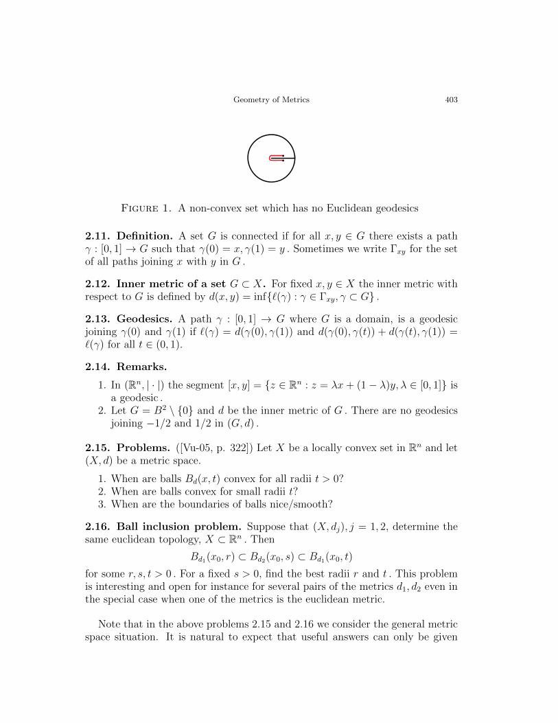
Figure 4. Hyperbolic lines are circular arcs perpendicular to ∂Bn

and ρBn(x, y) = log |x′, x, y, y′|.

For a given pair of points x, y ∈ Rn and a number t > 0 , an Apolloniansphere is the set of all points z such that |z − x|/|z − y| = t . It is easy to showthat, given x ∈ Bn , hyperbolic spheres with hyperbolic center x are Apollonianspheres w.r.t. the points x, x/|x|2, see [KV1].

Note that balls in chordal metric can be similarly described in terms of theeuclidean balls, see [AVV].

4.2. Hyperbolic metric of the unit ball Bn. Four equivalent definitionsof the hyperbolic metric ρBn .

1. ρBn = mw, w(x) = 21−|x|2 .

2. sinh2 ρBn (x,y)2

= |x−y|2(1−|x|2)(1−|y|2) .

3. ρBn(x, y) = sup{log |a, x, y, d| : a, d ∈ ∂Bn} .4. ρBn(x, y) = log |x∗, x, y, y∗| .

The hyperbolic metric is invariant under the action of GM(Bn), i.e. ρ(x, y) =ρ(h(x), h(y)) for all x, y ∈ Bn and all h ∈ GM(Bn) .

4.3. The hyperbolic line through x, y. The hyperbolic geodesics betweenx, y in the unit ball are the circular arcs joining x and y orthogonal to ∂Bn.

4.4. Hyperbolic metric of G = f(B2), f conformal. In the case where Gk =fk(B

2) and fk is conformal, k = 1, 2 , it follows that if h : G1 → G2 is conformal,then the hyperbolic metric is invariant under h , i.e., ρG1(x, y) = ρG2(hx, hy).Thus we may use explicit conformal maps to evaluate the hyperbolic metrics incases where such a map is known.


f conformal

-1f (y)

xy

-1f (x)

Figure 5. Definition of ρ(x, y) in terms of ρBn(f−1(x), f−1(y)),f conformal.

h

yh (x)

x h (y)

Figure 6. Invariance of the hyperbolic metric under conformal map.

For n = 2 one can generalize the hyperbolic metric, using covering transfor-

mations, to a domain G ⊂ R2with card(R2 \G) ≥ 3 [KL-07].

The formula for the hyperbolic metric of the unit ball given by 4.2(2) is rel-atively complicated. Therefore various comparison functions have been intro-duced. We will now discuss two of them.

4.5. The distance ratio metric jG. For x, y ∈ G the distance ratio metric jGis defined [Vu-85] by

jG(x, y) = log

(1 +

|x− y|min{d(x), d(y)}

).

The inequality jG ≤ δG ≤ jG ≤ 2jG holds for every open set G Rn, where themetric jG (cf. [GO-79]) is a metric defined by

jG(x, y) = log

(1 +|x− y|d(x)

)(1 +|x− y|d(y)

).

We collect the following well-known facts:

1. Inner metric of the jG metric is the quasihyperbolic metric kG .


2. kG(x, y) ≤ 2jG(x, y) for all x, y ∈ G with jG(x, y) < log(3/2) , see [Vu-88,3.7(2)].

3. Both kG and jG define the Euclidean topology.4. jG is not geodesic; the balls Bj(z,M) = {x ∈ G : jG(z, x) < M} may be

disconnected for large M .

If we compare the density functions of the hyperbolic and the quasihyperbolicmetrics of Bn, it will lead to the observations that

(4.5) ρBn(x, y)/2 ≤ kBn(x, y) ≤ ρBn(x, y)

for all x, y ∈ Bn .

The following proposition gathers together several basic properties of the met-rics kG and jG, see for instance [GP-76, Vu-88].

4.6. Proposition. ([KSV-09])

1. For a domain G ⊂ Rn, x, y ∈ G, and with L = inf{`(γ) : γ ∈ Γx,y} , wehave

kG(x, y) ≥ log

(1 +

L

min{δ(x), δ(y)}

)≥ jG(x, y) .

2. For x ∈ Bn we have

kBn(0, x) = jBn(0, x) = log1

1− |x|.

3. Moreover, for b ∈ Sn−1 and 0 < r < s < 1 we have

kBn(br, bs) = jBn(br, bs) = log1− r1− s

.

4. Let G Rn be any domain and z0 ∈ G. Let z ∈ ∂G be such thatδ(z0) = |z0 − z|. Then for all u, v ∈ [z0, z] we have

kG(u, v) = jG(u, v) =

∣∣∣∣logδ(z0)− |z0 − u|δ(z0)− |z0 − v|

∣∣∣∣ =

∣∣∣∣logδ(u)

δ(v)

∣∣∣∣ .5. For x, y ∈ Bn we have

jBn(x, y) ≤ ρBn(x, y) ≤ 2jBn(x, y)

with equality on the right hand side when x = −y .6. For 0 < s < 1 and x, y ∈ Bn(s) we have

jBn(x, y) ≤ kBn(x, y) ≤ (1 + s) jBn(x, y).


Proof. (1) Without loss of generality we may assume that δ(x) ≤ δ(y). Fixγ ∈ Γ(x, y) with arc length parameterization γ : [0, u]→ G, γ(0) = x, γ(u) = y

`k(γ) =

∫ u

0

|γ′(t)| dtd(γ(t), ∂G)

≥∫ u

0

dt

δ(x) + t= log

δ(x) + u

δ(x)

≥ log

(1 +|x− y|δ(x)

)= jG(x, y) .

(2) We see by (1) that

jBn(0, x) = log1

1− |x|≤ kBn(0, x) ≤

∫[0,x]

|dz|δ(z)

= log1

1− |x|and hence [0, x] is the kBn-geodesic between 0 and x and the equality in (2) holds.

The proof of (3) follows from (2) because the quasihyperbolic length is additivealong a geodesic

kBn(0, bs) = kBn(0, br) + kBn(br, bs) .

The proof of (4) follows from (3).

The proof of (5) is given in [AVV, Lemma 7.56].

For the proof of the last statement see [KSV-09].

In view of (4.5) and Proposition 4.6 we see that for the case of the unit ball,the metrics j, k, ρ are closely related.

5. Metrics in particular domains: uniform, quasidisks

We have seen above that for the case of the unit ball, several metrics areequivalent. This leads to the general question: Suppose that given a domainG ⊂ Rn we have two metrics d1, d2 on G . Can we characterize those domains G ,which for a fixed constant c > 0 satisfy d1(x, y) ≤ cd2(x, y) for all x, y ∈ G . Asfar as we know, this is a largely open problem. However, the class of domainscharacterized by the property that the quasihyperbolic and the distance ratiometric have a bounded quotient, coincides with the very widely known class ofuniform domains introduced by Martio and Sarvas [MS-79].

There is more general class of domains, so called ϕ-uniform domains, whichcontain the uniform domains as special case which we will briefly discuss [Vu-85].

It is easy to see that for a general domain the quasihyperbolic and distanceratio metrics both define the euclidean topology, in fact we can solve the ballinclusion problem 2.16 easily, see [Vu-88, (3.9)] for the case of the quasihyperbolicmetric. Although some progress has been made on this problem recently in[KV2], the problem is not completely solved in the case of metrics considered inthis survey.


5.1. Uniform domains and constant of uniformity. The following form ofthe definition of the uniform domain is due to Gehring and Osgood [GO-79].As a matter of fact, in [GO-79] there was an additive constant in the inequality(5.1), but it was shown in [Vu-85, 2.50(2)] that the constant can be chosen to be0 .

5.2. Definition. A domain G Rn is called uniform, if there exists a numberA ≥ 1 such that

(5.1) kG(x, y) ≤ AjG(x, y)

for all x, y ∈ G. Furthermore, the best possible number

AG := inf{A ≥ 1 : A satisfies (5.1)}is called the uniformity constant of G.

Our next goal is to explore domains for which the uniformity constant canbe evaluated or at least estimated. For that purpose we consider some simpledomains.

5.3. Examples of quasihyperbolic geodesics.

1. For the domain Rn\{0}Martin and Osgood (see [MO-86]) have determinedthe geodesics. Their result states that given x, y ∈ Rn \ {0}, the geodesicsegment can be obtained as follows: let ϕ be the angle between the segments[0, x] and [0, y], 0 < ϕ < π. The triple 0, x, y clearly determines a 2-dimensional plane Σ, and the geodesic segment connecting x to y is thelogarithmic spiral in Σ with polar equation

r(ω) = |x| exp

(ω

ϕlog|y||x|

).

In the punctured space the quasihyperbolic distance is given by the formula

kRn\{0}(x, y) =

√ϕ2 + log2 |x|

|y|.

2. [Lin-05] Let ϕ ∈ (0, π] and x, y ∈ Sϕ = {(r, θ) ∈ R2 : 0 < θ < ϕ}, theangular domain. Then the quasihyperbolic geodesic segment is a curveconsisting of line segments and circular arcs orthogonal to the boundary.If ϕ ∈ (π, 2π), then the geodesic segment is a curve consisting of piecesof three types: line segments, arcs of logarithmic spirals and circular arcsorthogonal to the boundary.

3. [Lin-05] In the punctured ball Bn \ {0}, the quasihyperbolic geodesic seg-ment is a curve consisting of arcs of logarithmic spirals and geodesic seg-ments of the quasihyperbolic metric of Bn.


1.2

1.2

1.2

1.21.4

1.4

1.4

1.4

1.6

1.6

1.6

1.6

1.6

1.8

1.8

1.8

1.8

2

222

2.2

2.2

2.2

2.4

2.4 2.6

−2 −1 0 1 2 3−2.5

−2

−1.5

−1

−0.5

0

0.5

1

1.5

2

2.5

Figure 7. Sets {z : kG(1, z)/jG(1, z) = c} .

The above formula 5.3(1) shows that the quasihyperbolic metric of G =Rn \ {0} is invariant under the inversion x 7→ x/|x|2 which maps G onto it-self. It is also easy to see that for this domain G also jB has the same invari-ance property. Next, for this domain G and a given number c > 1 , the sets{x : kG(1, x)/jG(1, x) = c} are illustrated. The invariance under the inversion isquite apparent. The same formula 5.3 (1) is also discussed in [KM].

We now give a list of constants of uniformity for a few specific domains fol-lowing H. Linden [Lin-05].

1. For the domain Rn \ {0}, the uniformity constant is given by (cf. Figure 7)

ARn\{0} = π/ log 3 ≈ 2.8596 .

2. Constant of uniformity in the punctured ball Bn \ {0} is same as that inRn \ {0}.

3. For the angular domain Sϕ, the uniformity constant is given by

ASϕ =1

sin ϕ2

+ 1

when ϕ ∈ (0, π].

There are numerous characterizations of quasidisks, i.e. quasiconformal im-ages of the unit disk under a quasiconformal map. E.g. it is known that a simplyconnected domain is a quasidisk if and only if it is a uniform domain, see [Ge-99].


5.4. ϕ-uniform domains ([Vu-85]). Let ϕ : [0,∞) → [0,∞) be a homeomor-phism. We say that a domain G ⊂ Rn is ϕ-uniform if

kG(x, y) ≤ ϕ(|x− y|/min{d(x, ∂G), d(y, ∂G)})

holds for all x, y ∈ G .

In [Vu-85] ϕ-uniform domains were introduced for the purpose of finding awide class of domains where various conformal invariants could be comparedto each other. Obviously, uniform domains form a subclass. Recently, manyexamples of these domains were given in [KSV-09]. This class of domains isrelative little investigated and there are many interesting questions even in thecase of plane simply connected ϕ-uniform domains. This class of plane domainscontains e.g. all quasicircles. Because for a quasicircle C the both componentsof C \ C are quasidisks, we could ask the following question. Suppose that Cis a Jordan curve in the plane dividing thus C \ C into two components, oneof which is a ϕ-uniform domain. Is it true that also the other component is aϕ1-uniform domain for some function ϕ1? This question was recently answeredin the negative in [HKSV-09].

5.5. Open problem. Is it true that there are ϕ-uniform domains G in theplane such that the Hausdorff-dimension of ∂G is two?

Recall that for quasicircles this is not possible by [GV]. P. Koskela has in-formed the author that Tomi Nieminen has done some work on this problem.

6. Hyperbolic type geometries

In this section we discuss briefly two metrics, the Apollonian metric αG and aMobius invariant metric δG introduced by P. Seittenranta [Se-99] and formulate afew open problems. For the case of the unit ball, both metrics coincide with thehyperbolic metric. For other domains they are quite different: while δG is alwaysa metric, for domains with small boundary αG may only be a pseudometric. TheApollonian metric was introduced in 1934 by D. Barbilian [Ba, BS], but forgottenfor many years. A. Beardon [Be-98] rediscovered it independently in 1998 andthereafter it has been studied very intensively by many authors: see, e.g., Z.Ibragimov [I], P. Hasto [Ha-03, Ha-04, Ha-05, Ha-04, HI-05, HPS-06, HKSV-09],S. Ponnusamy [HPWS-09, HPWW-10], S. Sahoo [SA]. See also D. Herron, W.Ma and D. Minda [HMM].


x y b

a

Figure 8. A quadruple of points admissible for the definition ofthe Apollonian metric.

6.1. Apollonian metric of G Rn.

αG(x, y) = sup{log |a, x, y, b| : a, b ∈ ∂G}.

• αG agrees with ρG, if G equals Bn and Hn.• αhG(hx, hy) = αG(x, y) for h ∈ GM(Rn)• αG is a pseudometric if ∂G is ”degenerate”

6.1.1. Facts.

1. The well-known sharp relations αG ≤ 2jG and αG ≤ 2kG are due to Beardon[Be-98].

2. αG does not have geodesics.3. The inner metric of the Apollonian metric is called the Apollonian inner

metric and it is denoted by αG (see [Ha-03, Ha-04, HPS-06]).4. We have αG ≤ αG ≤ 2kG.5. αG-geodesic exists between any pair of points in G Rn if Gc is not

contained in a hyperplane [Ha-04].

6.2. A Mobius invariant metric δG. For x, y ∈ G Rn, Seittenranta [Se-99]introduced the following metric

δG(x, y) = supa,b∈∂G

log{1 + |a, x, b, y|} .

6.2.1. Facts. [Se-99]

1. The function δG is a metric.2. δG agrees with ρG, if G equals Bn or Hn.3. It follows from the definitions that δRn\{a} = jRn\{a} for all a ∈ Rn.4. αG ≤ δG ≤ log(eαG + 2) ≤ αG + 3. The first two inequalities are best

possible for δG in terms of αG only [Se-99].


6.3. Open problem. Define

mBn(x, y) := 2 log

(1 +

|x− y|2 min{d(x), d(y)}

).

Then mBn(x, y) is not a metric. In fact, any choice of the points on a radialsegment will violate the triangle inequality. It is easy to see that kBn(x,−x) =mBn(x,−x). We do not know whether kBn(x, y) ≤ mBn(x, y) for all x, y ∈ Bn .If the inequality holds, then certainly kBn ≤ 2mBn ≤ 2jBn .

6.4. Diameter problems. There exists a domain G Rn and x ∈ G such thatj(∂Bj(x,M)) 6= 2M for all M > 0. Indeed, let G = Bn. Choose x ∈ (0, e1) andconsider the j-sphere ∂Bj(0,M) for M = jG(x, 0). Now, Bj(0,M) is a Euclideanball with radius |x| = 1− e−M . The diameter of the j-sphere ∂Bj(0,M) is

jG(x,−x) = log

(1 +|2x|d(x)

)= log

(1 +

2− 2e−M

e−M

)= log(2eM − 1) .

We are interested in knowing whether jG(x,−x) = 2M holds, equivalently in thiscase, (eM − 1)2 = 0 which is not true for any M > 0. Therefore, we always havejG(x,−x) < 2M and the diameter of ∂Bj(0,M) is less than twice the radius M .Note that there is no geodesic of the jG metric joining x and −x .

For a convex domain G, it is known by Martio and Vaisala [MV-08] thatk(∂Bk(x,M)) = 2M . However, we have the following open problem.

6.5. Open problem. Does there exist a number M0 > 0 such that for allM ∈ (0,M0] we have k(∂Bk(x,M)) = 2M . For the case of plane domains, thisproblem was studied by Beardon and Minda [BM-11].

6.6. Convexity problem [Vu-05]. Fix a domain G ( Rn and neohyperbolicmetric m in a collection of metrics (e.g. quasihyperbolic, Apollonian, jG, hyper-bolic metric of a plane domain etc.). Does there exist constant T0 > 0 such thatthe ball Bm(x, T ) = {z ∈ G : m(x, z) < T}, is convex (in Euclidean geometry)for all T ∈ (0, T0)?

6.7. Theorem. [[Kle-08]] For a domain G ( Rn and x ∈ G the j-balls Bj(x,M)are convex if and only if M ∈ (0, log 2].


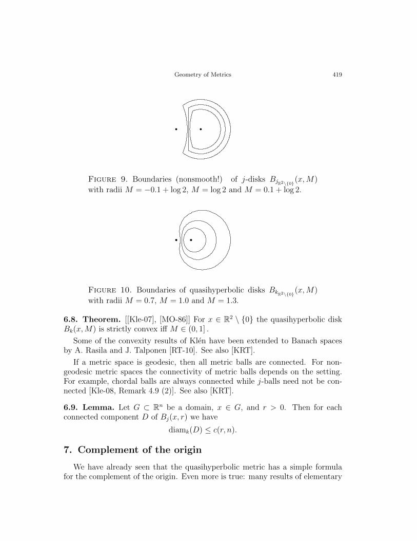
Figure 9. Boundaries (nonsmooth!) of j-disks BjR2\{0}(x,M)

with radii M = −0.1 + log 2, M = log 2 and M = 0.1 + log 2.

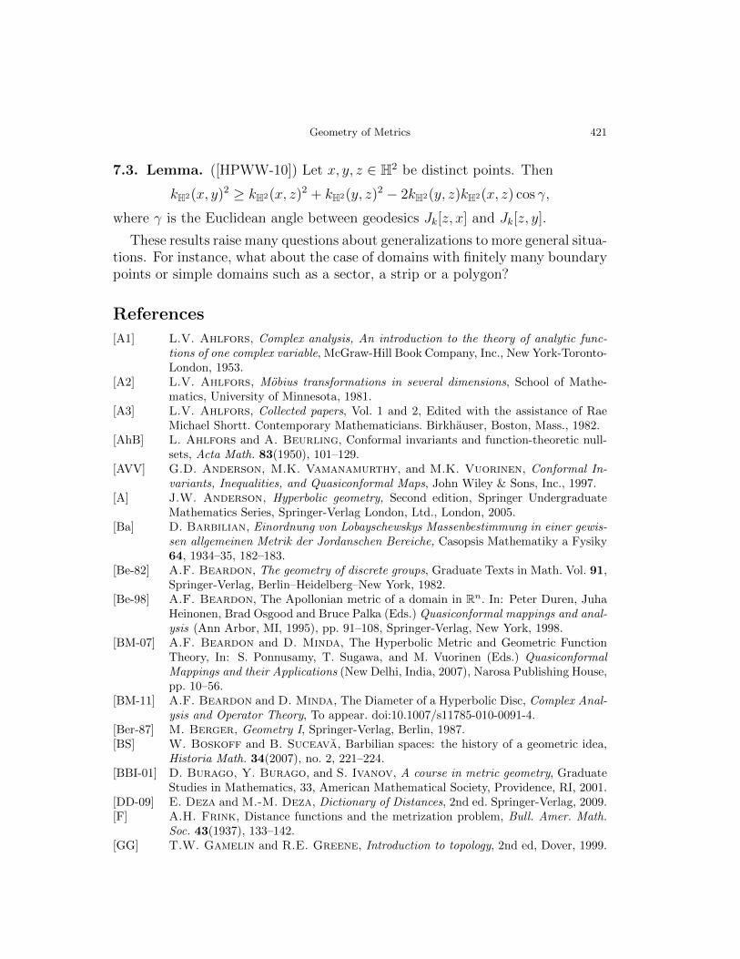
Figure 10. Boundaries of quasihyperbolic disks BkR2\{0}(x,M)

with radii M = 0.7, M = 1.0 and M = 1.3.

6.8. Theorem. [[Kle-07], [MO-86]] For x ∈ R2 \ {0} the quasihyperbolic diskBk(x,M) is strictly convex iff M ∈ (0, 1] .

Some of the convexity results of Klen have been extended to Banach spacesby A. Rasila and J. Talponen [RT-10]. See also [KRT].

If a metric space is geodesic, then all metric balls are connected. For non-geodesic metric spaces the connectivity of metric balls depends on the setting.For example, chordal balls are always connected while j-balls need not be con-nected [Kle-08, Remark 4.9 (2)]. See also [KRT].

6.9. Lemma. Let G ⊂ Rn be a domain, x ∈ G, and r > 0. Then for eachconnected component D of Bj(x, r) we have

diamk(D) ≤ c(r, n).

7. Complement of the origin

We have already seen that the quasihyperbolic metric has a simple formulafor the complement of the origin. Even more is true: many results of elementary


plane geometry hold, possibly with minor modifications, in the quasihyperbolicgeometry. Geometrically we can view (G, kG), G = R2 \ {0} as a cylindricalsurface embedded in R3, cf. [Kle-09].

Therefore many basic results of euclidean geometry hold for (G, kG) as suchor with minor modifications. Some of these results are listed below.

7.1. Theorem. [Law of Cosines] ([Kle-09]) Let x, y, z ∈ R2 \ {0}.(i) For the quasihyperbolic triangle 4k(x, y, z)

k(x, y)2 = k(x, z)2 + k(y, z)2 − 2k(x, z)k(y, z) cos]k(y, z, x).

(ii) For the quasihyperbolic trigon 4∗k(x, y, z)

k(x, y)2 = k(x, z)2 + k(y, z)2 − 2k(y, z)k(z, x) cos]k(y, z, x)− 4π(π − α),

where α = ](x, 0, y).

Figure 11. An example of a quasihyperbolic triangle (left) anda quasihyperbolic trigon (right). The small circle stands for thepuncture at the origin. [Kle-09]

7.2. Theorem. ([Kle-09]) Let 4k(x, y, z) be a quasihyperbolic triangle. Thenthe quasihyperbolic area of 4k(x, y, z) is√

s(s− k(x, y)

)(s− k(y, z)

)(s− k(z, x)

),

where s =(k(x, y) + k(y, z) + k(z, x)

)/2.

It is a natural question to ask whether for some other domains the Law ofCosines holds as an inequality, see [Kle-09]. For the case of the half plane theproblem was solved in [HPWW-10].


7.3. Lemma. ([HPWW-10]) Let x, y, z ∈ H2 be distinct points. Then

kH2(x, y)2 ≥ kH2(x, z)2 + kH2(y, z)2 − 2kH2(y, z)kH2(x, z) cos γ,

where γ is the Euclidean angle between geodesics Jk[z, x] and Jk[z, y].

These results raise many questions about generalizations to more general situa-tions. For instance, what about the case of domains with finitely many boundarypoints or simple domains such as a sector, a strip or a polygon?

References

[A1] L.V. Ahlfors, Complex analysis, An introduction to the theory of analytic func-tions of one complex variable, McGraw-Hill Book Company, Inc., New York-Toronto-London, 1953.

[A2] L.V. Ahlfors, Mobius transformations in several dimensions, School of Mathe-matics, University of Minnesota, 1981.

[A3] L.V. Ahlfors, Collected papers, Vol. 1 and 2, Edited with the assistance of RaeMichael Shortt. Contemporary Mathematicians. Birkhauser, Boston, Mass., 1982.

[AhB] L. Ahlfors and A. Beurling, Conformal invariants and function-theoretic null-sets, Acta Math. 83(1950), 101–129.

[AVV] G.D. Anderson, M.K. Vamanamurthy, and M.K. Vuorinen, Conformal In-variants, Inequalities, and Quasiconformal Maps, John Wiley & Sons, Inc., 1997.

[A] J.W. Anderson, Hyperbolic geometry, Second edition, Springer UndergraduateMathematics Series, Springer-Verlag London, Ltd., London, 2005.

[Ba] D. Barbilian, Einordnung von Lobayschewskys Massenbestimmung in einer gewis-sen allgemeinen Metrik der Jordanschen Bereiche, Casopsis Mathematiky a Fysiky64, 1934–35, 182–183.

[Be-82] A.F. Beardon, The geometry of discrete groups, Graduate Texts in Math. Vol. 91,Springer-Verlag, Berlin–Heidelberg–New York, 1982.

[Be-98] A.F. Beardon, The Apollonian metric of a domain in Rn. In: Peter Duren, JuhaHeinonen, Brad Osgood and Bruce Palka (Eds.) Quasiconformal mappings and anal-ysis (Ann Arbor, MI, 1995), pp. 91–108, Springer-Verlag, New York, 1998.

[BM-07] A.F. Beardon and D. Minda, The Hyperbolic Metric and Geometric FunctionTheory, In: S. Ponnusamy, T. Sugawa, and M. Vuorinen (Eds.) QuasiconformalMappings and their Applications (New Delhi, India, 2007), Narosa Publishing House,pp. 10–56.

[BM-11] A.F. Beardon and D. Minda, The Diameter of a Hyperbolic Disc, Complex Anal-ysis and Operator Theory, To appear. doi:10.1007/s11785-010-0091-4.

[Ber-87] M. Berger, Geometry I, Springer-Verlag, Berlin, 1987.[BS] W. Boskoff and B. Suceava, Barbilian spaces: the history of a geometric idea,

Historia Math. 34(2007), no. 2, 221–224.[BBI-01] D. Burago, Y. Burago, and S. Ivanov, A course in metric geometry, Graduate

Studies in Mathematics, 33, American Mathematical Society, Providence, RI, 2001.[DD-09] E. Deza and M.-M. Deza, Dictionary of Distances, 2nd ed. Springer-Verlag, 2009.[F] A.H. Frink, Distance functions and the metrization problem, Bull. Amer. Math.

Soc. 43(1937), 133–142.[GG] T.W. Gamelin and R.E. Greene, Introduction to topology, 2nd ed, Dover, 1999.


[Ge-99] F.W. Gehring, Characteristic properties of Quasidisks, Conformal geometry anddynamics, Banach Center Publications, 48, Ed. by B. Bojarski, J. Lawrynowicz, O.Martio, M. Vuorinen and J. Zajac, Institute of Mathematics, Polish Academy ofScience, Warszawa, 1999.

[Ge-05] F.W. Gehring, Quasiconformal mappings in Euclidean spaces, Handbook of com-plex analysis: geometric function theory, Vol. 2, ed. by R. Kuhnau, 1–29, Elsevier,Amsterdam, 2005.

[GH-00] F.W. Gehring and K. Hag, The Apollonian metric and Quasiconformal mappings,Contemp. Math. 256(2000), 143–163.

[GO-79] F.W. Gehring and B.G. Osgood, Uniform domains and the quasihyperbolicmetric, J. Anal. Math. 36(1979), 50–74.

[GP-76] F.W. Gehring and B.P. Palka, Quasiconformally homogeneous domains, J.Anal. Math. 30(1976), 172–199.

[GV] F.W. Gehring and J. Vaisala, Hausdorff dimension and quasiconformal map-pings, J. London Math. Soc. (2)6(1973), 504–512.

[Ha-03] P. Hasto, The Apollonian metric: uniformity and quasiconvexity, Ann. Acad. Sci.Fenn. Math. 28(2003), 385–414.

[Ha-04] P. Hasto, The Apollonian inner metric, Comm. Anal. Geom. 12(2004), no. 4,927–947.

[Ha-05] P. Hasto, Isometries of relative metrics, In: S. Ponnusamy, T. Sugawa, and M.Vuorinen (Eds.) Quasiconformal Mappings and their Applications, Narosa Publish-ing House, 57–77, New Delhi, India, 2007.

[HI-05] P. Hasto and Z. Ibragimov, Apollonian isometries of planar domains are Mobiusmappings, J. Geom. Anal. 15(2005), no. 2, 229–237.

[HKSV-09] P. Hasto, R. Klen, S.K. Sahoo, and M. Vuorinen, Geometric properties ofϕ-uniform domains, In preparation.

[HPS-06] P. Hasto, S. Ponnusamy, and S.K. Sahoo, Inequalities and geometry of theApollonian and related metrics, Rev. Roumaine Math. Pures Appl. 51(4)(2006),433–452.

[HE] V. Heikkala, Inequalities for conformal capacity, modulus, and conformal invari-ants, Ann. Acad. Sci. Fenn. Math. Diss. No. 132 (2002), 62 pp.

[HV-03] V. Heikkala and M. Vuorinen, Teichmuller’s extremal ring problem, Math. Z.254(2006), 509–529.

[Hei-01] J. Heinonen, Lectures on Analysis on Metric Spaces, Springer, 2001.[HMM] D. A. Herron, W. Ma, and D. Minda, Mobius invariant metrics bilipschitz

equivalent to the hyperbolic metric, Conform. Geom. Dyn. 12(2008), 67–96.[HPWS-09] M. Huang, S. Ponnusamy, X. Wang, and S.K. Sahoo, The Apollonian inner

metric and uniform domains, Math. Nachr. 283(2010), no. 9, 1277–1290.[HPWW-10] M. Huang, S. Ponnusamy, H. Wang, and X. Wang, A cosine inequality in

the hyperbolic geometry, Applied Mathematics Letters, 23(2010), 887–891.[I] Z. Ibragimov, The Apollonian metric, set of constant width and Mobius modulus

of ring domains, Ph. D. Thesis, University of Michigan, Ann Arbor, 2002.[KM] D. Kalaj and M. Mateljevic, Quasiconformal harmonic mappings and general-

izations, Manuscript, Jan. 2011.[KL-07] L. Keen and N. Lakic, Hyperbolic geometry from a local viewpoint, Cambridge

Univ. Press 2007.


[Kle-07] R. Klen, Local convexity properties of quasihyperbolic balls in punctured space,J. Math. Anal. Appl. J. 342(2008), 192–201.

[Kle-08] R. Klen, Local Convexity Properties of j-metric Balls, Ann. Acad. Sci. Fenn. Math.33(2008), 281–293.

[Kle-09] R. Klen, On hyperbolic type metrics, Ann. Acad. Sci. Fenn. Math. Disst. 152,2009.

[KRT] R. Klen, A. Rasila, and J. Talponen, Quasihyperbolic geometry in euclideanand Banach spaces, arXiv:1104.3745v1 [math.CV], 18 pp. 2010.

[KSV-09] R. Klen, S.K. Sahoo, and M. Vuorinen, Uniform continuity and ϕ-uniformdomains, arXiv:0812.4369 [math.MG], 21 pp, 2009.

[KV1] R. Klen and M. Vuorinen, Apollonian circles and hyperbolic geometry,arXiv:1010.2630 [math.MG], 21 pp, October 2010.

[KV2] R. Klen and M. Vuorinen, Inclusion relations of hyperbolic type metric balls,arXiv:1005.3927 [math.MG], 23 pp, May 2010.

[LV] O. Lehto and K.I. Virtanen, Quasiconformal mappings in the plane, Secondedition. Translated from the German by K. W. Lucas. Die Grundlehren der mathe-matischen Wissenschaften, Band 126. Springer-Verlag, New York-Heidelberg, 1973.viii+258 pp.

[Lin-05] H. Linden, Quasiconformal geodesics and uniformity in elementary domains, Ann.Acad. Sci. Fenn. Math. Diss. 146, 2005.

[Lin-05] H. Linden, Hyperbolic-type metrics, In: S. Ponnusamy, T. Sugawa, and M. Vuori-nen (Eds.), Quasiconformal Mappings and their Applications, Narosa PublishingHouse, 151–164, New Delhi, India, 2007.

[Man-08] V. Manojlovic, Moduli of Continuity of Quasiregular Mappings, Doctoral disser-tation, University of Belgrade, arXiv:0808.3241 [math.CA], 61 pp, 2008.

[Man-09] V. Manojlovic, On conformally invariant extremal problems, (English summary)Appl. Anal. Discrete Math. 3(2009), no. 1, 97–119.

[Mar-85] G. Martin, Quasiconformal and bilipschitz mappings, uniform domains and thehyperbolic metric, Trans. Amer. Math. Soc. 292(1985), 169–192.

[MO-86] G. Martin and B. Osgood, The quasihyperbolic metric and associated estimateson the hyperbolic metric, J. Anal. Math. 47(1986), 37–53.

[MS-79] O. Martio and J. Sarvas, Injectivity theorems in plane and space, Ann. Acad.Sci. Fenn. Math. 4(1979), 384–401.

[MV-08] O. Martio and J. Vaisala, Quasihyperbolic geodesics in convex domains II, PureAppl. Math. Q. 7(2011), 395–409.

[N-53] R. Nevanlinna, Eindeutige analytische Funktionen, - 2te Aufl. Die Grundlehrender mathematischen Wissenschaften in Einzeldarstellungen mit besondererBerucksichtigung der Anwendungsgebiete, Bd XLVI. Springer-Verlag, Berlin-Gottingen-Heidelberg, 1953.

[PS-09] M. Paluszynski and K. Stempak, On quasi-metric and metric spaces, Proc. Amer.Math. Soc. 137(2009), 4307–4312.

[RT-10] A. Rasila and J. Talponen, Convexity properties of quasihyperbolic balls onBanach spaces, arXiv:1007.3197v2 [math.CV], 15 pp, 2010.

[SA] S.K. Sahoo, Inequalities and geometry of hyperbolic-type metrics, radius problemsand norm estimates, Ph.D. Thesis, Indian Institute of Technology Madras, Chennai,2007, arXiv:1005.4317 [math.MG/math.CA], 155 pp, 2010.


[Se-99] P. Seittenranta, Mobius-invariant metrics, Math. Proc. Cambridge Philos.Soc. 125(1999), 511–533.

[V1] J. Vaisala, Lectures on n–dimensional quasiconformal mappings, Lecture Notes inMath. Vol. 229, Springer-Verlag, Berlin–Heidelberg–New York, 1971.

[V-99] J. Vaisala, The free quasiworld. Freely quasiconformal and related maps in Banachspaces, In: Quasiconformal geometry and dynamics (Lublin, 1996), Banach CenterPubl. 48, Polish Acad. Sci., Warsaw, 1999, pp. 55–118.

[V-09] J. Vaisala, Quasihyperbolic geometry of plane domains, Ann. Acad. Sci. Fenn.34(2009), 447–473.

[Vu-85] M. Vuorinen, Conformal invariants and quasiregular mappings, J. Anal.Math. 45(1985), 69–115.

[Vu-87] M. Vuorinen, On quasiregular mappings and domains with a complete conformalmetric, Math. Z. 194(1987) 459–470.

[Vu-88] M. Vuorinen, Conformal Geometry and Quasiregular Mappings, Lecture Notes inMathematics 1319, Springer-Verlag, Berlin–Heidelberg–New York, 1988.

[Vu-05] M. Vuorinen, Metrics and quasiregular mappings, In: S. Ponnusamy, T. Sugawa,and M. Vuorinen (Eds.) Quasiconformal Mappings and their Applications, NarosaPublishing House, 291–325, New Delhi, India, 2007.

[Vu4] M. Vuorinen, Geometric properties of quasiconformal maps and special functions,arXiv:0703687 [math.CV], 45 pp, 2007.

[Vu5] M. Vuorinen, Quasiconformal images of spheres, Mini-Conference on Quasiconfor-mal Mappings, Sobolev Spaces and Special Functions, Kurashiki, Japan, 2003-01-08.

Matti Vuorinen E-mail: [email protected]:Department of Mathematics,University of Turku,FIN-20014 Turku,Finland

Documents

Geometry of Metrics 1. Introduction